Embed Size (px)
Citation preview

This paper presents preliminary findings and is being distributed to economists
and other interested readers solely to stimulate discussion and elicit comments.
The views expressed in this paper are those of the authors and do not necessarily
reflect the position of the Federal Reserve Bank of New York or the Federal
Reserve System. Any errors or omissions are the responsibility of the authors.
Federal Reserve Bank of New York
Staff Reports
Business Cycle Fluctuations and the
Distribution of Consumption
Giacomo De Giorgi
Luca Gambetti
Staff Report No. 716
March 2015

Business Cycle Fluctuations and the Distribution of Consumption
Giacomo De Giorgi and Luca Gambetti
Federal Reserve Bank of New York Staff Reports, no. 716
March 2015
JEL classification: C3, D12, E21, E63
Abstract
This paper sheds new light on the interactions between business cycles and the consumption
distribution. We use Consumer Expenditure Survey data and a factor model to characterize the
cyclical dynamics of the consumption distribution. We first establish that our approach is able to
closely match business cycle fluctuations of consumption from the National Account. We then
study the responses of the consumption distribution to total factor productivity shocks and
economic policy uncertainty shocks. Importantly, we find that the responses of the right tail of the
consumption distribution, mostly comprising more highly educated individuals, to shocks that
drive cyclical fluctuations are larger and quicker than in other parts of the distribution. We note
that the cost of business cycle fluctuations is larger than that found using aggregate consumption
and that the shocks we analyze reduce consumption inequality on impact.
Key words: consumption, inequality, cost of business cycles, heterogeneity, aggregate shocks,
structural factor model, FAVAR
_________________
De Giorgi: Federal Reserve Bank of New York (e-mail: [email protected]).
Gambetti: Universitat Autònoma de Barcelona and Barcelona Graduate School of Economics
(e-mail: [email protected]). The authors thank Rodica Calmuc and Michela Giorcelli for
very skillful research assistance. Financial support from the Spanish Ministry of Science and
Innovation through grant ECO2009-09847 and the Barcelona Graduate School Research Network
is gratefully acknowledged. De Giorgi acknowledges financial support from the Spanish Ministry
of Economy and Competitiveness, through the Severo Ochoa Programme for Centres of
Excellence in R&D (SEV-2011-0075) and ECO2011-28822, and the EU through the Marie Curie
CIG grant FP7-631510. The views expressed in this paper are those of the authors and do not
necessarily reflect the position of the Federal Reserve Bank of New York or the Federal Reserve
System.

1 Introduction
How does the consumption distribution evolve over the business cycle? How do shocks
that drive economic fluctuations affect the consumption distribution? What are the
cyclical properties of consumption inequality? Is exposure to the business cycle different
across consumers? Answering these questions is a priority for the design of sensible
and effective economic policies. Indeed in recent years several authors have stressed
the importance of going beyond the representative agent framework by allowing some
type of heterogeneity across consumers for meaningful welfare analysis (for a review, see
Heathcote, Storesletten and Violante, 2009, Guvenen, 2011). Krusell, Mukoyama, Sahin,
and Smith (2009), using a calibrated model for the US, show that the cost of business
cycles is substantially different across consumers: very poor and rich consumers would
gain substantially more than other consumers from the removal of cyclical fluctuations.
On the empirical front there is a substantial amount of work documenting trends
in economic inequality, see for example Heathcote, Perri and Violante (2010a) and the
literature cited therein. In that paper the authors analyze long run trends of inequality
in wages, income and consumption over the last four decades in the US and show that the
increase in consumption inequality has been much more moderate than that of wages
and disposable incomes. A more recent literature finds that consumption inequality
tracks income inequality more closely than previously thought, see for example Attanasio,
Hurst, and Pistaferri (2012), and Attanasio and Pistaferri (2014).
The evidence on the relation between the consumption distribution and the busi-
ness cycle is more limited. A few papers have studied the dynamics of inequality during
downturns. Consumption inequality tend to increase much less than earnings and income
inequality during recessions, see Krueger, Perri, Pistaferri and Violante (2010). In par-
ticular Parker and Vissing-Jorgensen (2009) and Heathcote, Perri and Violante (2010b)
show that the Great Recession has initially reduced inequality due to the pronounced
reduction of consumption of the 10th decile.
This paper provides a systematic empirical investigation aimed at shedding new light
on the interactions between business cycles and the consumption distribution. We use
CEX data to construct household level non-durable consumption (expenditures), using
this measure we then calculate the mid-points of the different deciles of the consumption
distribution for each quarter over the period 1984Q1-2010Q4. Our empirical analysis
is carried out using a structural factor model (Bernanke, Boivin and Eliasz 2005, and
Forni, Giannone, Lippi and Reichlin 2009). The model provides a unified framework to
model a large amount of macroeconomic data together with the consumption deciles.
Each series is modeled as the sum of two orthogonal components: the common and
the idiosyncratic components. The former is driven by the macroeconomic shocks with
1

pervasive effects on the economy, while the latter by series specific events unrelated to
macro shocks (e.g. taste differences or measurement error in the consumption deciles).
We characterize the cyclical dynamics of the common component of the consumption
deciles and study the response of the consumption distribution to both a TFP and an
economic policy uncertainty shock. Finally we check the validity of our econometric
approach using simulated data.
The main findings are as follows. First, the common component of aggregate CEX
consumption tracks aggregate consumption from the National Account (NIPA Tables)
remarkably well at the business cycle frequencies. This is striking since the literature
has extensively documented that the two aggregate series are substantially different in
several respects. The reason why we obtain a close match between the two series is that
our model can correct for a relatively general idiosyncratic component. Second, at the
business cycle frequencies the top end of the distribution is much more volatile, suggesting
a higher exposure of high-consumption individuals to economic fluctuations. The result
suggests a higher cost of the business cycle for consumers in the right tail, about three
times larger than for other consumers. Third, while the left tail of the distribution follows
GDP with a lag of about two to three quarters, the right tail anticipates GDP by one to
two quarters. The finding suggests that not only the exposure but also the decision rules
are different across consumers, which gives rise to different consumption cycles. Fourth,
TFP and economic policy uncertainty shocks have significantly higher effects on the
top end of the distribution. Both shocks generate pro-cyclical movement in consumption
inequality. Fifth, when using educational categories to split the consumption distribution
rather than the deciles of consumption, we find that more educated individuals tend to
respond to a larger extent and more quickly to the business cycle.
In trying to assess potential explanations that can account for the heterogeneity in
behavior pointed out by these results, we find substantial heterogeneity across consumers
in terms of expectations. More specifically, we find that highly educated individuals
tend to forecast future economic conditions much better than other consumers. While
expectations indeed play a role, we are not able to tell whether different consumers have
different expectations or simply different information sets. Also, expectations are unlikely
to explain the whole story. For instance, it is reasonable to think of the existence of
rigidities and market imperfections, like liquidity constraints, which give rise to different
decision rules.
The remainder of the paper is organized as follows: Section 2 introduces the econo-
metric model. Section 3 describes the data used, and presents the results. Section 4
describes a set of simulations to assess the validity of the econometric approach. Sec-
tion 5 discuss the identification of the TFP and the uncertainty shocks and presents the
results. Section 6 provides a discussion of the results. Section 7 concludes.
2

2 The model
In this section we describe our empirical model. The starting point is a model for indi-
vidual consumption. Individual consumption is the sum of two orthogonal components,
a common aggregate component and an idiosyncratic component. The common compo-
nent is driven by common aggregate shocks while the idiosyncratic part includes shocks
which do not have pervasive effects on the economy. Given that a panel is not available
for individual consumption, we aggregate individual consumption data to construct the
deciles of the consumption distribution and we derive the implied empirical model for
the (mid-points of) consumption deciles.
Consumption cjt1 of individual j, for j = 1, ..., n, is given by
cjt = ajft + εjt (1)
where ft is a r × 1 vector of of macroeconomic factors, aj is the individual response
to aggregate economic conditions and εjt is a stationary idiosyncratic shock orthogonal
to ft capturing all the determinants of individual consumption unrelated to aggregate
conditions , e.g. health, luck or measurement error. Apart from stationarity we do not
make any additional assumption about εjt.
We then aggregate individual consumption data into deciles and take the mid-point
of each decile. The model for the ith decile is then written as:
cit = acift + ξcit (2)
where cit =∑ni
j=1 cjtni
, aci =∑ni
j=1 ajni
ξcit =∑ni
j=1 εjtni
. Also the decile-specific consumption is
driven by two orthogonal components: the common component acift and the idiosyncratic
component ξit. Notice that aci is now the average response of consumption in group i to
macroeconomic factors. The latter includes unrestricted decile-specific shocks and mea-
surement error which can accommodate differential measurement errors across deciles,
since for example the measurement error is likely higher at the top of the distribution.
The dynamic relation between consumption units and macroeconomic shocks arises
from the fact that the vector ft follows a VAR structure:
N(L)−1ft = Sut, (3)
where ut is a r-dimensional vector of orthonormal white noise structural macroeconomic
shocks, i.e. productivity shocks, policy shocks etc., and N(L) a r × r matrix of polyno-
mials in the lag operator L with N(0) = I.
1Here there is a little abuse of notation. The index j in the cjt should have an index t in that the
jth consumer in two different periods are different individuals. However for sake of simplicity and to
facilitate the exposition we abstract from this complication
3

Using (2) and (3) we have
cit = bci (L)ut + ξcit (4)
where bci (L) = aciN(L)S. The first term on the right-hand side of equation (4), bci (L)ut,
describes the relation between consumption units and the macroeconomy. Macroeco-
nomic shocks are dynamically transmitted to consumption through the impulse response
functions bci (L).
In order to estimate the unobserved elements of ft we assume a factor structure for
the whole economy. More specifically, every macroeconomic variable xit, for i = 1, ...,m
is the sum of two mutually orthogonal components, the common component and the
idiosyncratic component
xit = axi ft + ξxit (5)
where the common component is again driven by common aggregate macroeconomic
shocks
axi ft = bxi (L)ut (6)
where bxi (L) = axiN(L)S. The idiosyncratic component, ξxit, in this case should be
interpreted as measurement error for variables like GDP, or sectoral shocks in the case
of sectoral variables. Following Bernanke, Boivin and Eliasz (2006), we allow for the
possibility of having s observed factors in ft. Let fot be the vector of observed factors
and fut of unobserved factors. The unobserved factors ft are estimated by means of the
first r − s principal components of the variables xit in the dataset. The factor loading
aci and axi are estimated by regressing cit and xit respectively onto ft.
In Appendix A we list all the variables used for estimating the factors and their trans-
formations. The deciles of consumptions are taken in logs for the sake of interpretation.2
3 The dynamics of the consumption distribution
3.1 CEX data and summary statistics
We construct household (non-durable) consumption from CEX data: 1984Q1 to 2010Q4.
The CEX records consumption and expenditure for a large set of goods together with
demographics and other households characteristics. Following a number of papers, see
for example Attanasio and Weber (1995), Krueger and Perri (2006), Attanasio, Bat-
tistin, and Padula (2009), Parker and Vissing-Jorgensen (2009), we focus exclusively on
household nondurable consumption expenditure per adult equivalent in real terms.3 In
2We have also used the deciles of the log distribution and the results are qualitatively the same. The
results are not reported in the paper but are available upon request.3We use an equivalence scale suggested by the World Bank, i.e. we divide our relevant variables by
the squared root of the number of household members. We use the standard CPI to deflated the series.
4

the construction of the non-durable consumption variable we strictly follow the defini-
tion used in Attanasio and Weber (1995).4 For each quarter we build the consumption
distribution from the CEX microdata, applying the population weights provided therein.
We then identify the different deciles and take the mid-points of each decile.5 We note
that there are, on average, around 200 households within each decile/quarter cell.
Figure 1 shows some summary statistics of the deciles of the (log) consumption
distribution. The top left panel plots the standard deviation of the raw data. It is clearly
noticeable how the two tails of the distribution are more volatile than the central part of
the distribution. In particular, the 10th decile is twice as volatile as the middle deciles.
The top right panel displays the share of the variance of each decile attributable to the
common component. For robustness, we plot these shares for 3 different specifications:
using 6 (solid line), 10 (dashed line), and 16 (dotted line) Principal Components (PC).
We note how “commonality” is substantially larger for central deciles. However, as shown
in the bottom panels of Figure 1, for the raw data both the common (bottom left panel)
and the idiosyncratic (bottom right panel) components are substantially more volatile
at the top end of the distribution.
3.2 NIPA and CEX at the business cycle frequencies
We begin our analysis with a comparison between the NIPA and CEX aggregate non-
durable consumption. Overtime the tracking between the CEX and the National Account
statistics on aggregate consumption has been fading. A number of papers have described
such occurrence and tried, with mixed results, to reconcile the two series or analyze the
differences between the two measures of aggregate consumption (see for example Garner,
2006, Goldenberg and Ryan, 2009, Battistin and Padula, 2010, Aguiar and Bils, 2011,
Attanasio and Pistaferri, 2014).
The upper panel of Figure 2 plots the cyclical component of the NIPA consumption
(dotted line) and the cyclical component of the aggregate CEX (solid line). To compute
the two series we apply a band-pass filter retaining only business cycle fluctuations (from
1.5 to 8 years). Fluctuations in the two series are substantially different, the correlation
being around 0.5. Moreover the variance of the CEX aggregate is substantially larger
4In particular we refer to the following definition from Attanasio and Weber (1995): “...In what follows
we consider various components of nondurable expenditure. In particular, for reasons to be discussed
below, we look at food (defined as the sum of food at home, food away from home, alcohol, and tobacco)
and expenditure on other nondurable goods and services, such as services, heating fuel, public and private
transport (including gasoline), and personal care, and semidurables, defined as clothing and footwear...”5Results are robust to assign each household to a given decile once and for all by ordering households
mean consumption expenditure overtime. As a typical household is observed for 3 quarters, this in
practice means that we average household consumption over that time period and we order that average
to locate each household in the appropriate decile.
5

than the NIPA counterpart.
The lower panel of Figure 2 plots the cyclical component of the NIPA consumption
(dotted line) and the cyclical component of the common component of the aggregate
CEX (solid line). The latter is obtained by applying the above filter to the common
component of the CEX aggregate.6 The two series track each other remarkably well, with
a correlation coefficient of around 0.8. This shows that once the idiosyncratic component
is removed from the data, the remaining common component displays fluctuations which
are very similar to those observed in the NIPA aggregate.
A few remarks are in order. First, there is a non-negligible part of persistent fluctua-
tions in the CEX which is idiosyncratic. This is one of the reason why it has been hard to
reconcile the two series even at the business cycle frequencies. Second, the result is not a
mechanic implication of the factor model. Although both series are driven by a common
component, the correlation between the two series could in principle be zero given that
the number of principal components is larger than one. Third, our claim is that only
fluctuations at the business cycle frequencies in the two components are similar and not
the two series in general. Importantly for our analysis, we note that any differences
between the CEX and NIPA aggregate common components series are orthogonal to the
business cycle, i.e. it is not true that CEX common component systematically over or
underestimate NIPA common component in booms or downturns.
We believe that the finding presented in this section is extremely important. On the
one hand it is the first piece of evidence documenting that the two series can track each
others remarkably well. On the other hand it is an important validation of our modeling
strategy and suggests that our approach can be successfully employed to investigate
business cycle fluctuation using CEX consumption data.
3.3 One, two, three consumption cycles
Figure 3 plots the correlations at various leads and lags of the cyclical component of GDP
with the cyclical component of the common component of the deciles, i.e. the band-pass
filtered component of acitft. The x-axis refers to the lags and leads of the deciles. The
correlations are remarkably high for all the deciles, with a minimum for the 1st decile of
0.77 and a maximum for the 10th decile of 0.87. Conversely, the dynamic structure is
very different across deciles. While the left tail of the distribution follows GDP with a lag
of about two to three quarters, the right tail anticipates GDP by one to two quarters.7
A similar message emerges from Figure 4, where we plot the cyclical component of the
GDP (dashed line) together with the cyclical component of the common component
6Nondurables CEX aggregate consumption is one of the series of the macroeconomic dataset so we
can compute the common component.7The same finding is confirmed either using the NIPA or CEX aggregate consumption.
6

of the consumption deciles (solid line). The 10th decile leads while lower deciles lag
the fluctuations in the GDP. These results suggest that there are actually three cycles
which are similar in amplitude but differ by a phase shift. Fluctuations in GDP follow
fluctuations in the 10th decile with a delay of two quarters and fluctuations in the left
tail of the distribution follows GDP fluctuations with a lag of about three quarters.
Figure 5 reports the variance at cyclical frequencies of the common component of
the consumption deciles rescaled by the variance of the aggregate CEX consumption.
The volatility of the central deciles is similar in magnitude to that of CEX aggregate
consumption while the 1st and 10th deciles are much more volatile, their variances being
about two and three times larger than the aggregate consumption, respectively.
The findings discussed above point out two important facts. First, the exposure to
cyclical fluctuations is different across deciles. It is much higher in the right tail and, to a
substantially lesser extent, in the left tail than for mid-deciles. This has two implications
in terms of the cost of cyclical fluctuations. First, the business cycle is more costly for
the two tails, in particular the right one. Second, the cost of the business cycle measured
solely with aggregate data can be substantially underestimated. Indeed we aggregate the
volatilities of the different deciles using as weights the ratio of the consumption decile
over total consumption (the sum of the deciles). We find that the cost is 40% higher
than that obtained using only the volatility of aggregate consumption, the weighted sum
of the decile variances is 1.64 while the variance of the CEX agregate is only 1.18.8 The
result is in line with the theoretical predictions in Mankiw and Zeldes (1991) where the
consumption of the stockholders, i.e. the wealthy consumers, is much more volatile, and
with the work of Krusell et al. (2009). However, it is in contrast with a large body of
theoretical models where wealthy consumers tend to smooth consumption much more
than poor consumers who behave in a hand-to-mouth fashion; notable exceptions are
Parker and Vissing-Jorgensen (2009), and Parker (2014).
The second fact, implied by the correlation structure of the consumption deciles
and GDP, is that average decision rules (within decile) are substantially different across
deciles. The right tail moves first, pushing aggregate consumption and GDP, and then
the rest of the distribution follows with a lag that is increasing as we look at the left
part of the distribution. This latter fact will be discussed in detail in section 6.
4 Simulations
We run a series of simulations in order to assess whether our econometric strategy is
able to correctly estimate true heterogeneity in the common component which we model
in the data generating process. In other words, we test whether our procedure is able to
8Following Lucas (1987) we measure the cost as λ = 12σ2θ.
7

correctly estimate the true decile effects, aci . We generate individual-level consumption
data from model (1) where the only common component is the growth rate of GDP. We
construct the decile of the consumption distribution and then we regress the decile on
the growth rate of GDP and get an estimate of aci . Finally we compare the true value
of aci used in the data generating process and its estimates. The simulation is done for
different type of heterogeneity, i.e. values of ai, and different idiosyncratic processes.
The simulation works as follows:
1. We generate n = 2000 (corresponding to the average number of consumers in
the survey per time period) different individual consumption paths of T = 108
observations (corresponding to the time length of our data) from the equation
cjt = αj + aj∆ log(GDPt) + ξjt ξjt ∼ N(0, σ2jt).
where ∆ log(GDPt) is the common component and ξjt is the idiosyncratic compo-
nent. Notice that the idiosyncratic component is very general, since its variance
can differ both across individuals and across time.
2. We compute the deciles of the consumption distribution, we regress each decile on
∆ log(GDPt) and estimate the mean response aci .
We parametrize the model as follows. The constant term is αj = 1 + jn/10 . The constant
ranks consumers according to their expected conditional level of consumption. Individual
1 is the one with the lowest level of consumption, while individual 2000 is the one with
the highest one. The variance of the idiosyncratic component, ξjt, is random and has
a Gamma distribution σ2jt ∼ Gamma(6, β) with scale parameter equal to 6 and shape
parameter β.9 We run the simulation for β = 1, 2,√
10. Basically to generate cjt,
t = 1, ..., T we draw T realizations of σjt and T realizations of ξjt.
Simulation #1. We assume that high-consumption individuals have a larger response
to GDP growth and set aj = jn . Top panel of Figure 6 reports the true mean values
aci (solid line), and the estimated values in the three simulations aci , (dashed β = 1,
dotted β = 4, dashed-dotted dotted β = 10). When β = 1 the parameters are estimated
remarkably well. The distortion increases with the size of β. Two remarks are in order.
For β = 1 the mean of the variance of ξjt is already 6, about 15 times larger than the
variance of ∆ log(GDPt) which is 0.36. For β = 2,√
10 the variance of the idiosyncratic
component is unreasonably large. In the sensible case β = 1 the model does very
well. Second, the distortion drives to overestimating the response of the left tail and
underestimating the response of the right tail. In other words, for extremely large values
9We consider a Gamma distribution since has positive support and the scale and the shape parameters
allow us to play wit the mean and the variance of the distribution.
8

of β our procedure would underestimate the degree of heterogeneity of the consumption
deciles.
In our simulation, individual consumers at the top of the distribution are more ex-
posed to GDP growth then other consumers, meaning that the common component is
more important at the top. However, when the idiosyncratic component is very large the
deciles analysis tells a different story. The bottom panel of Figure 7 plots the percentage
of variance of the deciles attributable to the common component for β = 1 (dashed line),
β = 2 (dotted line) and β =√
10 (dashed-dotted line). For β = 2 and β =√
10, the
percentage of variance of the 10th decile accounted for by the common component is
lower than that of the middle deciles. Therefore, one could falsely conclude that top
consumers are more idiosyncratic, which is at odds with the true prediction. There are
two implications: first, it is not advisable to interpret the percentage of common variance
of the distribution deciles as the common variance of the individuals within the decile;
second, although the individual-level idiosyncratic component is on average equal for all
the consumers, the idiosyncratic shock for the decile can be substantially different across
deciles.
Simulation #2. We assume all the individuals have the same response to GDP growth
and set aj = a = 1 for j = 1, ..., n. Results are reported in the mid panel of Figure 6. In
this case our procedure would correctly capture a constant coefficient across deciles.10
Simulation #3. We assume that low-consumption individuals have a larger response
to GDP growth and set aj = 1− j−1n . Results are reported in the bottom panel of Figure
6. Results are similar to those reported in Simulation 1. When β = 1 the parameters
are estimated relatively well and the distortion increases with the size of β.
5 Shocks
So far the analysis has focused on the unconditional dynamics of the consumption deciles.
Here we turn our attention on how the consumption distribution responds to economic
shocks. We focus on two different shocks: a standard TFP shock and an economic policy
uncertainty shock. We focus our attention to these two shocks since in the literature,
they have been considered serious candidates to explain cyclical fluctuations (see Kidland
and Prescott, 1982, among many others for TFP shocks and Bloom, 2009, and Baker,
Bloom, and Davis, 2012).
10We also tried with a random coefficient uniformly distributed in [0, 1] and the for all the deciles the
estimates are around 0.5.
9

5.1 TFP shock
Identification proceeds as follows. First, we assume that total factor productivity (TFP)
is the only observable factor and is ordered first in ft. We estimate the VAR for the
factors and we identify the shock as an innovation in the VAR equation for the TFP.11.
More formally let Σ be the variance covariance matrix of the innovation εt = Sut in the
VAR equation N(L)−1ft = Sut. Let S be the Cholesky factor of Σ. The shock is the
first shock of the vector ut = S−1εt. The first element of aciN(L)S and axiN(L)S are
the impulse response functions of cit and xit respectively. An estimated of N(L)−1 is
obtained by inverting the matrix of estimated VAR coefficients obtained with OLS. An
estimate of S is obtained as the Cholesky factor of the estimated covariance matrix of
the VAR residuals. This provides an estimate for N(L)−1S.
Figure 7 plots the impulse response functions of main macroeconomic aggregates to
a positive TFP shock. The solid line is the point estimate, the grey area represents the
68% confidence bands. The shock has the typical business cycles effects. It generates a
protracted and significant increase in GDP, consumption, and investment, and a persis-
tent reduction of the unemployment rate while and the federal funds rate barely moves.
Notice that the responses of CEX and NIPA non-durables consumption are quite similar.
Figure 8 reports the effects of the shock on the consumption deciles (x-axis). The
upper left panel reports the average effect over the first year after the shock. The
upper right panel reports the effects over the second year. The lower left panel reports
the average effects over the third year after the shock. The lower right panel reports
the average effect over the first 3 years. During the first year after the shock (upper-
left panel), consumption increases only at the very top of the distribution, only the
10th decile responds positively and significantly. The response of the left part of the
distribution is virtually zero. In the second year (upper-right panel), the left tail of the
distribution catches up, the effects on the first two deciles being significantly different
from zero. In the third year (lower-left panel) the effects are zero.
The top panel of Figure 9 plots the response of inequality, measured as the difference
between the responses of the 10th decile and the 1st decile. Inequality increases signifi-
cantly during the first two periods. The bottom panel of Figure 9 plots the variance of
each decile attributable to the TFP shock rescaled by the variance of the CEX aggre-
gate attributable to the TFP shock. The measure, as before, provides some evidence for
the heterogeneity of the cost of cyclical fluctuations across deciles. The finding suggests
that the cost for the 10th decile is significantly larger than that obtained for aggregate
consumption (rescaled variance is significantly larger than one).
The main takeaway here is that TFP shocks have substantially larger effects at the
11This is the way standard technology shock is identified in Barsky and Sims (2011).
10

top of the consumption distribution.
5.2 Economic policy uncertainty shock
Identification of the economic policy uncertainty shock is implemented as before but
replacing the TFP series with the economic policy uncertainty measure of Baker, Bloom,
and Davis (2012). The shock is the innovation in the uncertainty equation, the first
equation in the VAR for the factors.
Figure 10 plots the impulse response functions of main macroeconomic aggregates
to a positive uncertainty shock (an increase in uncertainty). The shock has the typical
business cycles effects: GDP, consumption, and investment increase, unemployment falls
and the federal funds rate barely moves. Again the responses of CEX and NIPA non-
durables consumption are quite similar.
Figure 11 reports the effects of the shock on the consumption deciles (x-axis). As
before, within the first year after the shock, consumption reduces significantly only at
the top of the distribution, the effects on the other deciles being not significant. In the
second and third year consumption at the top continues significantly below its pre-shock
level but now also the other consumption deciles reduce. So while in the short run only
the left tail responds to the shock, at longer horizons all the distribution shifts to the
left. The result replicates what we have found above. The left tail moves first and then
the remainder of the distribution follows with a lag.
The top panel of Figure 12 plots the response of inequality. Inequality falls by 1%
on impact and by about 0.5% for the first two years. The confidence bands however
are quite large and the effect is not significantly different from 0 at the 68% confidence
level. The bottom panel of Figure 9 plots the variance of the deciles attributable to
the uncertainty shock rescaled by the variance of the CEX aggregate attributable to the
shock. As for the TFP shock analysis, the rescaled variance is significantly larger than
one only for the 10th decile.
Ultimately, results for a policy uncertainty shock are similar to those for the TFP
shock. The right tail reacts to either shock with greater magnitude and speed.
5.3 Evidence using educational categories
We provide additional evidence for the effects of TFP and uncertainty shocks on con-
sumption using CEX data aggregated by educational categories, and in particular by
the highest level of education reached by the household head. We aggregate the data by
four educational categories: less than high school; high school; some college; college and
beyond education. This has the advantage of constructing a consumption series based
on a permanent characteristic, i.e. education.
11

In Table 1, we show the composition of the different consumption deciles in terms of
education. As one would expect the bottom decile is made up mostly of lower education
household heads. For example, up to the third decile at least 60% of individuals have
at most a high school education. At the same time, the top 4 deciles are composed
of individuals with at least some college education. It is quite interesting that in the
bottom decile we still find that the college educated make up about 7% of the decile,
and that in the top decile about 5% of the individuals have below high-school education.
In this analysis, we employ the factor model developed in the previous sections, but we
replace the dependent variable substituting the consumption deciles with the average
household consumption by education category. We then apply the same identification
strategy used in the previous two sections for the two shocks. Figure 13 plots the impulse
response functions of the four education categories (rows) to the TFP shock (left column)
and the uncertainty shock (right column). The response of highly educated individuals’
consumption is much larger and more instantaneous than that of the other categories.
This essentially confirms the previous analysis based on the classification of consumption
by decile.
6 Discussion
Our findings robustly point out that the right tail of the consumption distribution and
the consumption of the more educated individuals respond more and more quickly to
shocks that drive cyclical fluctuations. The natural question arising from our finding is:
what explains this heterogeneity? We believe there could be a number of explanations
for this behavior, and here we focus on two, non-mutually exclusive, explanations. The
first explanation is that consumers at the top of the distribution, those in the 9th and
10th decile, form expectations in a very different way from the rest of the individuals. In
particular they seem to be much more forward looking and sensitive to future expected
economic conditions (Armantier et al., 2014). To investigate such a possibility we use
data from Michigan Survey of Consumers. We restrict our attention to two expecta-
tion variables: (i) the expected consumer sentiment index (ICE); and (ii) the expected
business conditions over the next 12 months (BUS12).12
We use data for the two variables aggregated by educational categories. For each
variable we have 5 series corresponding to the following educational categories: less than
high school, high school, some college, college and graduate studies. We also consider
as an alternative, and for robustness, the aggregation by income quartiles. We forecast
one-quarter ahead the year on year growth rate of GDP with each variable. The forecast
of the GDP growth from t to t + 1, say ∆GDPt+1|t is simply the value at time t of
12See Appendix for the precise definitions of the two variables.
12

ICE and BUS12. We compute forecast errors as ∆GDPt+1 − ∆GDPt+1|t and we run
the Diebold and Mariano test for any pair of forecast. For instance we compare the
forecast made using ICE for the high school category with the forecast made with ICE
for the college categories. The null hypothesis is that the two forecasts produce the same
forecasting accuracy.
Table 2a displays the Diebold and Mariano statistics along with the p-values of the
test. First, the results for the two variables, BUS12 and ICE are remarkably similar.
Second, the forecast accuracy increases with the level of education, all the statistics
except college versus graduate studies are positive. Third, the forecasts of the first
category are significantly less accurate than all the other categories. Fourth, also high
school graduates do predict worse than higher categories, although the difference in the
forecasts are not significant.
Table 2b displays the results for income categories. Forecast accuracy of the bottom
25% is significantly lower than that of the other quartiles. The second quartile also
predicts worse than the third and the top quartile. The ICE and the DM statistics of
the second versus the fourth is significant at the 10% level. Concluding, highly educated
(wealthier) individuals are better at predicting their own consumption and the business
cycle.
The findings suggest that there are significant differences in the accuracy of the
forecast of future growth rates of GDP across individuals. This can explain, to some
extent, the differences in the reaction of consumption across deciles. However what
remains an intriguing open question is whether the differences also depend on different
classes of expectations, general heterogeneity, or simply different information sets.
Expectations, however, are likely to be only part of the story. A second plausible
explanation is that there are rigidities and market imperfections, such as liquidity con-
straints, which prevent consumer in the left and center of the distribution from promptly
reacting to the new information about future economic conditions. Establishing the rela-
tive importance of the two explanations is undoubtedly interesting but beyond the scope
of this paper.
7 Conclusions
In this paper we analyze the behavior of consumption across the business cycle for the
past 30 years, allowing for heterogenous behavior of consumers across two dimensions:
i. consumption deciles, and ii. education.
A number of important facts emerge from our analysis: first, we are able to capture
quite well the aggregate business cycle behavior of the NIPA aggregate consumption
using consumption measured from CEX microdata. This result is crucial for our analysis,
13

but more importantly because allows policy analysis on business cycle consumption at
the individual level or at a minimum at some more disaggreagated level then the NIPA
aggregate level, which is somewhat limited for policy purposes. Second, we show how the
business cycle common component of fluctuations is quite heterogenous across consumers
and as such we show that welfare losses from business cycle fluctuations are actually non-
trivial when one looks at the more detailed picture. Third, we show that the cyclical
responses to the business cycles follow a very different dynamic for the bottom and top
consumers. While top consumers move ahead of the cycle and respond more strongly,
bottom consumers move with two to three quarters lag and have a much milder responses.
Fourth, TFP as well as economic uncertainty shocks have much larger effects on top
consumers. Fifth, one explanation we can give is that top (highly educated) consumers
are much better at forecasting economic conditions and as such respond promptly to
changing circumstances. From a policy perspective our analysis is crucial as it shows
how aggregate shocks have very different impacts on different consumers. Ultimately, it
is the role of policy to decide whether and with whom to intervene, without the type of
analysis implemented in this paper that would essentially be an unfounded call.
14

References
[1] Aguiar, Mark and Mark Bils, (2011). ”Has Consumption Inequality Mirrored In-
come Inequality?” NBER Working Paper 16807.
[2] Armantier, O., Bruine de Bruin, W., Topa, G. and, van der Klaauw, W., (2014),
”Inflation Expectations and Behavior: Do Survey Respondents Act on their Be-
liefs?”, forthcoming, the International Economic Review.
[3] Attanasio, Orazio, James Bank, and Sarah Tanner (2002). ”Asset holding and con-
sumption volatility” Journal of Political Economy, 110 (4), 771792.
[4] Attanasio, Orazio, Erich Battistin, and Vincenzo Padula, (2009). ”Inequality in
Living Standards since 1980: Evidence from Expenditure Data” Mimeo.
[5] Attanasio, Orazio, Erik Hurst, and Luigi Pistaferri, (2012), “The evolution of in-
come, consumption, and leisure inequality in the US, 1980-2010,” NBER Working
Papers: 17982.
[6] Attanasio, Orazio, and Luigi Pistaferri, (2014), “Consumption inequality over the
last half century. Evidence using the new PSID consumption measure”, American
Economic Review P&P, 104(5): 112-126.
[7] Attanasio, Orazio and Guglielmo Weber, (1995). ”Is Consumption Growth Consis-
tent with Intertemporal Optimization? Evidence from the Consumer Expenditure
Survey” Journal of Political Economy, 103(6):11211157.
[8] Baker, Scott, Nicholas Bloom, and Steve Davis (2012). ”Measuring economic policy
uncertainty”. Stanford University mimeo.
[9] Barsky, Robert B. and Eric, R. Sims (2011). ”News shocks and business cycles,”
Journal of Monetary Economics 58(3):273-289.
[10] Battistin, Erich and Mario Padula (2010). ”Survey Instruments and the Reports
of Consumer Expenditures: Evidence from the Consumer Expenditure Surveys”
Mimeo, IFS.
[11] Bernanke Ben, Jean Boivin and Piotr Eliasz, (2005). ”Measuring Monetary Policy:
A Factor Augmented Autoregressive (FAVAR) Approach” The Quarterly Journal
of Economics, 120:387422.
[12] Bloom, Nick, (2009). ”The Impact of Uncertainty Shocks” Econometrica,
77(3):623685.
15

[13] Forni Mario, Domenico Giannone, Marco Lippi, and Lucrezia Reichlin, (2009).
”Opening the Black Box: Structural Factor Models with Large Cross-Sections”
Econometric Theory, 25:13191347.
[14] Goldenberg, Karen and Jay Ryan,(2009). ”Evolution and Change in the Consumer
Expenditure Surveys: Adapting Methodologies to Meet Changing Needs, BLS.
[15] Guvenen, Fatih, (2011). ”Macroeconomics with Heterogeneity: A Practical Guide”
Economic Quarterly, 97:255326.
[16] Heathcote, Jonathan, Fabrizio Perri, and Giovanni L. Violante (2010a). ”Unequal
We Stand: An Empirical Analysis if Economic Inequality in the US, 19672006”
Review of Economic Dynamics 13(1): 1551.
[17] Heathcote, Jonathan, Fabrizio Perri, and Giovanni L. Violante (2010b). ”Inequality
in Times of Crisis: Lessons from the Past and a First Look at the Current Recession’
VoxEU.org, February 2.
[18] Heathcote, Jonathan, Kjetil Storesletten, and Giovanni L. Violante, (2009). ”Quan-
titative Macroeconomics with Heterogeneous Households” Annual Review of Eco-
nomics, 1:319354.
[19] Kydland, Finn E and Edward C. Prescott, (1982). ”Time to Build and Aggregate
Fluctuations” Econometrica 50(6):1345-1370.
[20] Krueger, Dirk and Fabrizio Perri, (2006). ”Does income inequality lead to consump-
tion inequality? Evidence and theory” Review of Economic Studies, 73(1):163193.
[21] Krueger, Dirk, Fabrizio Perri, Luigi Pistaferri, and Giovanni L. Violante. (2010).
”Cross-Sectional Facts for Macroeconomists” Review of Economic Dynamics 13(1):
114.
[22] Krusell, Per and Anthony Smith, (1999). ”On the Welfare Effects of Eliminating
Business Cycles” Review of Economic Dynamics, 2(1):245272.
[23] Krusell, Per, Toshihiko Mukoyama, Aysegul Sahin and Anthony A. Smith, Jr.,
(2009). ”Revisiting the Welfare Effects of Eliminating Business Cycles,” Review
of Economic Dynamics, Elsevier for the Society for Economic Dynamics, vol.
12(3):393-402.
[24] Lucas, Robert, (1987). ”Models of Business Cycles”.
[25] Mankiw, Gregory and Stephen P. Zeldes, (1991). ”The consumption of stockholders
and nonstockholders” Journal of Financial Economics, 29:97112.
16

[26] Parker, Jonathan A. and Annette Vissing-Jorgensen, “Who Bears the Aggregate
Fluctuations and How?,” working paper Northwestern University, 2009.
[27] Parker, Jonathan A., “Why Don’t Households Smooth Consumption? Evidence
from a 25 million dollar experiment,” mimeo MIT, 2014.
[28] Primiceri, Giorgio and Thijs van Rens (2005). ”Heterogeneous Life-Cycle Pro-
files, Income Risk and Consumption Inequality”, Journal of Monetary Economics,
56(1):20-39.
[29] Stock, James H. and Mark W. Watson, Implications of Dynamic Factor Models for
VAR Analysis, NBER Working Papers no. 11467, 2005.
17

Appendix A
Transformations: 1=levels, 2= first differences of the original series, 5= first differences of logs of the original
series.
no.series Transf. Mnemonic Long Label
1 5 GDPC1 Real Gross Domestic Product, 1 Decimal
2 5 GNPC96 Real Gross National Product
3 5 NICUR/GDPDEF National Income/GDPDEF
4 5 DPIC96 Real Disposable Personal Income
5 5 OUTNFB Nonfarm Business Sector: Output
6 5 FINSLC1 Real Final Sales of Domestic Product, 1 Decimal
7 5 FPIC1 Real Private Fixed Investment, 1 Decimal
8 5 PRFIC1 Real Private Residential Fixed Investment, 1 Decimal
9 5 PNFIC1 Real Private Nonresidential Fixed Investment, 1 Decimal
10 5 GPDIC1 Real Gross Private Domestic Investment, 1 Decimal
11 5 PCECC96 Real Personal Consumption Expenditures
12 5 PCNDGC96 Real Personal Consumption Expenditures: Nondurable Goods
13 5 PCDGCC96 Real Personal Consumption Expenditures: Durable Goods
14 5 PCESVC96 Real Personal Consumption Expenditures: Services
15 5 GPSAVE/GDPDEF Gross Private Saving/GDP Deflator
16 5 FGCEC1 Real Federal Consumption Expenditures & Gross Investment, 1 Decimal
17 5 FGEXPND/GDPDEF Federal Government: Current Expenditures/ GDP deflator
18 5 FGRECPT/GDPDEF Federal Government Current Receipts/ GDP deflator
19 2 FGDEF Federal Real Expend-Real Receipts
20 1 CBIC1 Real Change in Private Inventories, 1 Decimal
21 5 EXPGSC1 Real Exports of Goods & Services, 1 Decimal
22 5 IMPGSC1 Real Imports of Goods & Services, 1 Decimal
23 5 CP/GDPDEF Corporate Profits After Tax/GDP deflator
24 5 NFCPATAX/GDPDEF Nonfinancial Corporate Business: Profits After Tax/GDP deflator
25 5 CNCF/GDPDEF Corporate Net Cash Flow/GDP deflator
26 5 DIVIDEND/GDPDEF Net Corporate Dividends/GDP deflator
27 5 HOANBS Nonfarm Business Sector: Hours of All Persons
28 5 OPHNFB Nonfarm Business Sector: Output Per Hour of All Persons
29 5 UNLPNBS Nonfarm Business Sector: Unit Nonlabor Payments
30 5 ULCNFB Nonfarm Business Sector: Unit Labor Cost
31 5 WASCUR/CPI Compensation of Employees: Wages & Salary Accruals/CPI
32 5 COMPNFB Nonfarm Business Sector: Compensation Per Hour
33 5 COMPRNFB Nonfarm Business Sector: Real Compensation Per Hour
34 5 GDPCTPI Gross Domestic Product: Chain-type Price Index
35 5 GNPCTPI Gross National Product: Chain-type Price Index
36 5 GDPDEF Gross Domestic Product: Implicit Price Deflator
37 5 GNPDEF Gross National Product: Implicit Price Deflator
38 5 INDPRO Industrial Production Index
39 5 IPBUSEQ Industrial Production: Business Equipment
40 5 IPCONGD Industrial Production: Consumer Goods
41 5 IPDCONGD Industrial Production: Durable Consumer Goods
42 5 IPFINAL Industrial Production: Final Products (Market Group)
43 5 IPMAT Industrial Production: Materials
44 5 IPNCONGD Industrial Production: Nondurable Consumer Goods
45 2 AWHMAN Average Weekly Hours: Manufacturing
46 2 AWOTMAN Average Weekly Hours: Overtime: Manufacturing
18

no.series Transf. Mnemonic Long Label
47 2 CIVPART Civilian Participation Rate
48 5 CLF16OV Civilian Labor Force
49 5 CE16OV Civilian Employment
50 5 USPRIV All Employees: Total Private Industries
51 5 USGOOD All Employees: Goods-Producing Industries
52 5 SRVPRD All Employees: Service-Providing Industries
53 5 UNEMPLOY Unemployed
54 5 UEMPMEAN Average (Mean) Duration of Unemployment
55 2 UNRATE Civilian Unemployment Rate
56 5 HOUST Housing Starts: Total: New Privately Owned Housing Units Started
57 2 FEDFUNDS Effective Federal Funds Rate
58 2 TB3MS 3-Month Treasury Bill: Secondary Market Rate
59 2 GS1 1-Year Treasury Constant Maturity Rate
60 2 GS10 10-Year Treasury Constant Maturity Rate
61 2 AAA Moody’s Seasoned Aaa Corporate Bond Yield
62 2 BAA Moody’s Seasoned Baa Corporate Bond Yield
63 2 MPRIME Bank Prime Loan Rate
64 5 BOGNONBR Non-Borrowed Reserves of Depository Institutions
65 5 TRARR Board of Governors Total Reserves, Adjusted for Changes in Reserve
66 5 BOGAMBSL Board of Governors Monetary Base, Adjusted for Changes in Reserve
67 5 M1SL M1 Money Stock
68 5 M2MSL M2 Minus
69 5 M2SL M2 Money Stock
70 5 BUSLOANS Commercial and Industrial Loans at All Commercial Banks
71 5 CONSUMER Consumer (Individual) Loans at All Commercial Banks
72 5 LOANINV Total Loans and Investments at All Commercial Banks
73 5 REALLN Real Estate Loans at All Commercial Banks
74 5 TOTALSL Total Consumer Credit Outstanding
75 5 CPIAUCSL Consumer Price Index For All Urban Consumers: All Items
76 5 CPIULFSL Consumer Price Index for All Urban Consumers: All Items Less Food
77 5 CPILEGSL Consumer Price Index for All Urban Consumers: All Items Less Energy
78 5 CPILFESL Consumer Price Index for All Urban Consumers: All Items Less Food & Energy
79 5 CPIENGSL Consumer Price Index for All Urban Consumers: Energy
80 5 CPIUFDSL Consumer Price Index for All Urban Consumers: Food
81 5 PPICPE Producer Price Index Finished Goods: Capital Equipment
82 5 PPICRM Producer Price Index: Crude Materials for Further Processing
83 5 PPIFCG Producer Price Index: Finished Consumer Goods
84 5 PPIFGS Producer Price Index: Finished Goods
85 5 OILPRICE Spot Oil Price: West Texas Intermediate
86 5 USSHRPRCF US Dow Jones Industrials Share Price Index (EP) NADJ
87 5 US500STK US Standard & poor’s Index if 500 Common Stocks
88 5 USI62...F US Share Price Index NADJ
89 5 USNOIDN.D US Manufacturers New Orders for Non Defense Capital Goods (BCI 27)
90 5 USCNORCGD US New Orders of Consumer Goods & Materials (BCI 8) CONA
91 1 USNAPMNO US ISM Manufacturers Survey: New Orders Index SADJ
92 5 USVACTOTO US Index of Help Wanted Advertising VOLA
93 5 USCYLEAD US The Conference Board Leading Economic Indicators Index SADJ
94 5 USECRIWLH US Economic Cycle Research Institute Weekly Leading Index
95 2 GS10-FEDFUNDS
96 2 GS1-FEDFUNDS
97 2 BAA-FEDFUNDS
19

no.series Transf. Mnemonic Long Label
98 5 GEXPND/GDPDEF Government Current Expenditures/ GDP deflator
99 5 GRECPT/GDPDEF Government Current Receipts/ GDP deflator
100 2 GDEF Governnent Real Expend-Real Receipts
101 5 GCEC1 Real Government Cons. Expenditures & Gross Investment, 1 Decimal
102 5 Real Federal Cons. Expenditures & Gross Investment National Defense
103 2 Federal primary deficit
104 5 Real Federal Current Tax Revenues
105 5 Real Government Current Tax Revenues
106 2 Government primary deficit
107 5 Real (/GDPDEF) Gov. Social Benefit
108 1 Gov. social benefits/ Gov. Curr Exp
20

Appendix B
ICE is constructed as a weighted average of three variables BUS12, BUS5 and DUR.
The three variables measure the percentage of responses reporting good future condi-
tions minus the percentage of responses reporting bad future conditions the following
questions:
BUS12: ”Now turning to business conditions in the country as a whole–do you
think that during the next twelve months we’ll have good times financially, or bad
times, or what”
BUS5: ”Looking ahead, which would you say is more likely–that in the country as
a whole we’ll have continuous good times during the next five years or so, or that
we will have periods of widespread unemployment or depression, or what”
DUR: ”About the big things people buy for their homes–such as furniture, a re-
frigerator, stove, television, and things like that. Generally speaking, do you think
now is a good or bad time for people to buy major household items?”.
21

Tables
decile < HS HS Some col. >=College Total
1 40.64 33.74 17.67 7.95 100.00
2 27.96 38.45 20.61 12.98 100.00
3 20.60 38.40 22.54 18.46 100.00
4 15.67 38.62 23.33 22.37 100.00
5 12.32 37.25 23.35 27.08 100.00
6 10.12 34.93 23.58 31.37 100.00
7 7.98 32.69 23.25 36.08 100.00
8 6.63 30.28 22.26 40.83 100.00
9 5.34 26.37 21.25 47.05 100.00
10 5.57 25.50 20.85 48.08 100.00
Table 1: composition of the consumer deciles in terms of educational attainments.
22

BUS12 ICE
HS Some col. College Graduate < HS Some col. College Graduate
< HS 2.45 2.31 2.56 2.72 2.56 2.34 2.83 2.77
(p-value) (0.01) (0.01) (0.01) (0.00) (0.01) (0.01) (0.00) (0.00)
HS 0.26 1.28 1.07 -0.20 1.42 0.86
(p-value) (0.40) (0.10) (0.14) (0.58) (0.08) (0.19)
Some col. 1.28 0.82 2.05 1.12
(p-value) (0.10) (0.21) (0.02) (0.13)
College -0.21 -0.85
(p-value) (0.58) (0.80)
Table 2a: Diebold and Mariano statistics for education categories. The forecast produced
by each variable listed in the first column is tested against the forecast produced by the
variables listed in the first row of the other columns. The null hypothesis is that the the
forecasting accuracy is equal for the two forecast considered. p-values are displayed in
parenthesis.
BUS12 ICE
Second 25% Third 25% Top 25% Second 25% Third 25% Top 25%
Bottom 25% 2.65 1.96 2.39 2.86 2.87 3.25
(p-value) (0.00) (0.03) (0.01) (0.00) (0.00) (0.00)
Second 25% 0.10 1.07 0.88 1.58
(p-value) (0.46) (0.14) (0.19) (0.06)
Third 25% 1.50 1.10
(p-value) (0.07) (0.14)
Table 2b: Diebold and Mariano statistics for income categories. The forecast produced
by each variable listed in the first column is tested against the forecast produced by the
variables listed in the first row of the other columns. The null hypothesis is that the the
forecasting accuracy is equal for the two forecast considered. p-values are displayed in
parenthesis.
23

Figures
Figure 1:. Summary statistics of the deciles of the consumption distribution. Top left
panel – standard deviation of raw data. The top right panel – percentage of variance
of the deciles attributable to the common component. Bottom left panel – standard
deviation of the common component. The bottom right panel – standard deviation of
the idiosyncratic component. Solid line – 6 principal components; the dashed line – 10
principal components. Dotted line – 16 principal components.
24

Figure 2. Upper panel – cyclical component of the NIPA consumption (dotted line) and
cyclical component of the aggregate CEX (solid line). Lower panel: cyclical component
of the NIPA consumption (dotted line) and cyclical component of the common component
of the aggregate CEX (solid line).
25

Figure 3. Correlations between lags and leads of the cyclical common components of the
consumption deciles and the cyclical components of GDP. On the x-axis there are the
lags (negative values) and the leads (positive values) of the consumption deciles. Each
panel also displays the maximal correlation.
26

Figure 4. Cyclical component of the GDP (dashed line) and the cyclical component of
the common component of the deciles (solid line).
27

Figure 5. Variance at cyclical frequencies of the common component of the consumption
deciles rescaled by the variance of the aggregate CEX consumption.
28

Figure 6. Top panel simulation # 1. True mean values aci (solid line), and the estimated
values aci , (dashed β = 1, dotted β = 4, dashed-dotted dotted β = 10). Bottom panel:
percentage of variance of the decile variance accounted for by the common component:
dashed β = 1, dotted β = 4, dashed-dotted dotted β = 10). Deciles on the x-axis.
29

Figure 7. Top panel simulation # 2. True mean values aci (solid line), and the estimated
values aci , (dashed β = 1, dotted β = 4, dashed-dotted dotted β = 10). Lower panel
simulation # 3. True mean values aci (solid line), and the estimated values aci , (dashed
β = 1, dotted β = 4, dashed-dotted dotted β = 10).
30

Figure 7. Impulse response functions of macroeconomic variables to a positive TFP
shock. Solid line – point estimates; grey area – 68% confidence bands.
31

Figure 8. Impulse response functions of consumption deciles (x-axis) to a positive TFP
shock. The upper left panel – average effect over the first year after the shock. The
upper right panel – effects over the second year. The lower left panel – average effects
over the third year after the shock. The lower right panel – average effect over the first
3 years. Solid line – point estimates; grey area – 68% confidence bands.
32

Figure 9. Top panel: response of inequality, measured as the difference between the
response of the 10th decile and the 1st decile, to a TFP shock. Bottom panel: variance
of each deciles attributable to the TFP shock rescaled by the variance of the CEX
aggregate attributable to the TFP shock. Solid line – point estimates; grey area – 68%
confidence bands.
33

Figure 10. Impulse response functions of consumption deciles (x-axis) to en economic
uncertainty shock. The upper left panel – average effect over the first year after the
shock. The upper right panel – effects over the second year. The lower left panel –
average effects over the third year after the shock. The lower right panel – average effect
over the first 3 years. Solid line – point estimates; grey area – 68% confidence bands.
34
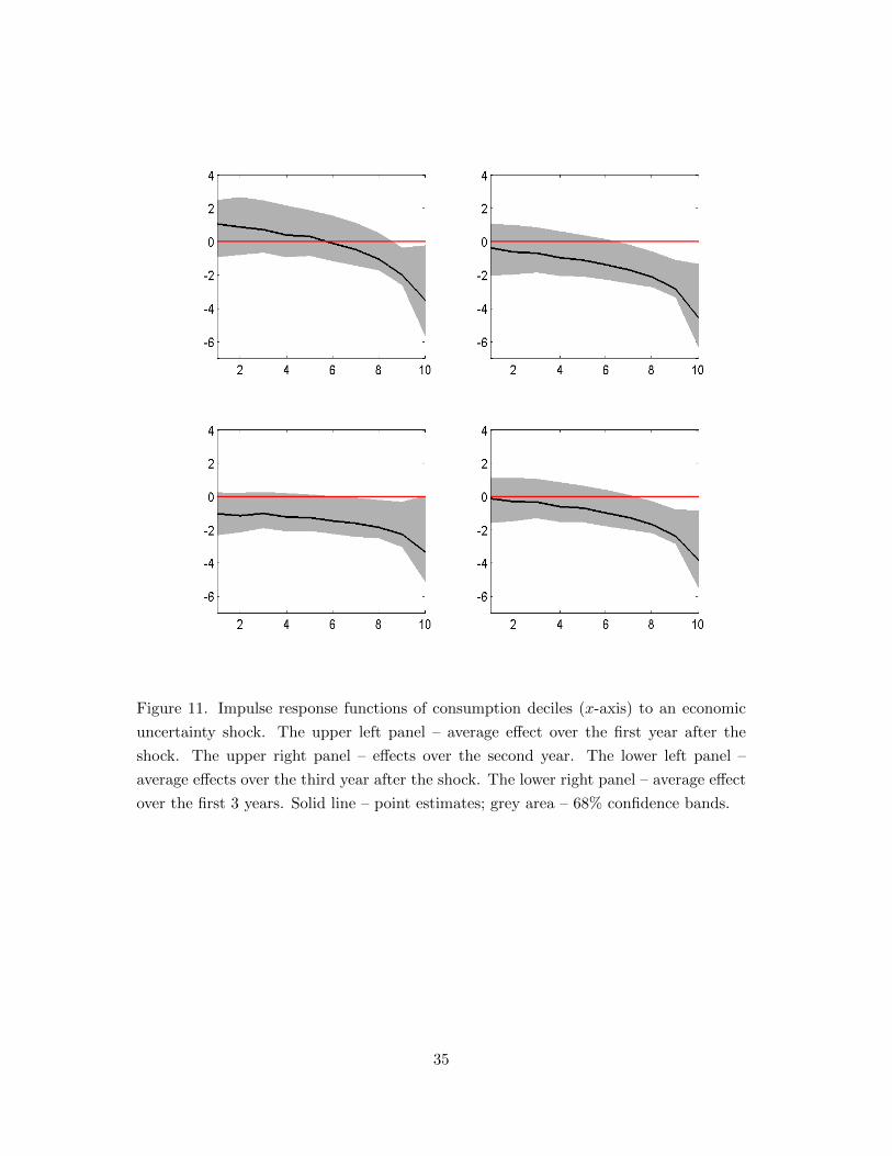
Figure 11. Impulse response functions of consumption deciles (x-axis) to an economic
uncertainty shock. The upper left panel – average effect over the first year after the
shock. The upper right panel – effects over the second year. The lower left panel –
average effects over the third year after the shock. The lower right panel – average effect
over the first 3 years. Solid line – point estimates; grey area – 68% confidence bands.
35

Figure 12. Top panel: response of inequality, measured as the difference between the
response of the 10th decile and the 1st decile, to an economic uncertainty shock. Bottom
panel: variance of each deciles attributable to the TFP shock rescaled by the variance
of the CEX aggregate attributable to the TFP shock. Solid line – point estimates; grey
area – 68% confidence bands.
36

Figure 13. Impulse response functions of the four education categories to the TFP shock
(left column) and economic uncertainty shock (right column). First row – less than high
school (< HS); second row – high school (HS); third row – some college (Some col.);
fourth row – college and graduate studies (>=College). Solid line – point estimates;
grey area – 68% confidence bands.
37


![[Untitled] []— Stock, James and Mark Watson (1999). "Business Cycle Fluctuations in U.S. Macroeconomic Time Series." In Handbook of Macroeconomics: 3-64. Real Business Cycle Model:](https://img.pdfslide.us/doc/110x75/60e25badd6f4b450d67c8534/untitled-a-stock-james-and-mark-watson-1999-business-cycle-fluctuations.jpg)