Bureaucrats, voters, and public investment

Journal of Public Economics 119 (2014) 35–48

Contents lists available at ScienceDirect

Journal of Public Economics

j ourna l homepage: www.e lsev ie r .com/ locate / jpube

Bureaucrats, voters, and public investment☆

Levon Barseghyan, Stephen Coate ⁎Department of Economics, Cornell University, Ithaca NY 14853, United States

☆ We thank Aaron Bodoh-Creed, Francesco Trebbi, anvery helpful comments.⁎ Corresponding author.

E-mail addresses: [email protected] (L. Barseghyan),1 This literature is a subbranch of the vast body of work

imentally, and empirically alternative arrangements for pcontributions include Bowen (1943) and Bergstrom (197der majority rule, Lizzeri and Persico (2001, 2005) on pmulti-party political competition, Baron (1996) and Voldeislative provision, and Niskanen (1971) and Romer and Rreaucratic provision.

http://dx.doi.org/10.1016/j.jpubeco.2014.07.0090047-2727/© 2014 Elsevier B.V. All rights reserved.

a b s t r a c t
a r t i c l e i n f o
Article history:Received 21 December 2012Received in revised form 7 July 2014Accepted 24 July 2014Available online 8 August 2014

Keywords:Agenda controlDurable public goodBudget maximizing bureaucrat

This paper explores the provision of a durable public good in Romer and Rosenthal's agenda setter model. Itidentifies a type of equilibrium, called a Romer–Rosenthal equilibrium, in which in every period the bureaucratproposes themaximum level of public investment the voterwill support. The paper establishes that such an equi-librium exists for a variety of public good benefit functions. Equilibrium public good levels converge or almostconverge to a steady state. These steady states can involve a unique public good level being provided each periodor may exhibit a two period cycle. Steady state public good levels exceed the voter's optimal level. More surpris-ingly, steady state equilibrium reversion levels can exceed the voter's optimal steady state level, meaning thatreversion levels cannot be used to bound the optimal level. Reflecting the inability of the agents to commit totheir future proposing and voting behavior, equilibrium paths are Pareto inefficient.

© 2014 Elsevier B.V. All rights reserved.

1. Introduction

A central focus of research on the theory of public goods has beenunderstanding the performance of different political processes in pro-viding such goods.1 The major goal of this research has been to under-stand how political decision-making distorts provision away from thenormative ideal. The motivation is both to better understand realworld policy outcomes and to provide insights concerning the relativemerits of different political institutions. The bulk of this literature has fo-cused on the provision of static public goods, such as firework displaysandpolice protection,whichmust be provided aneweachperiod. In prac-tice, however, many important public goods are durable, lasting formanyyears and depreciating relatively slowly. Public infrastructure, defense ca-pability, and environmental quality are good examples. Understandingthe political provision of such goods is more challenging, because oftheir durable nature. Today's political choices have implications for futurechoices, creating a dynamic linkage across policy-making periods.

The practical importance of durable public goods and the theoreticalchallenges they pose has led to increased interest in their political pro-vision. For example, a number of recent papers have studied the

d two anonymous referees for

[email protected] (S. Coate).exploring theoretically, exper-

ublic good provision. Important9) on public good provision un-rovision under two party andn and Wiseman (2007) on leg-osenthal (1978, 1979b) on bu-

provision of such goods by legislatures when tax revenues can also beused to finance district-specific transfers (Battaglini and Coate, 2007;Battaglini et al., 2012; Leblanc et al., 2000). This paper contributes tothe developing literature on the political provision of durable publicgoods by exploring their determination in Romer and Rosenthal's agen-da setter model (Romer and Rosenthal, 1978, 1979b). This well-knownmodel offers a lens through which to understand the spending of localgovernments.2 It studies the interaction between a bureaucrat whomanages the provision of a public good or service for a communityand the citizens in that community. The level of the public good is cho-sen by the bureaucrat but is subject to citizen approval via a ratificationvote. If the bureaucrat's proposed spending level is not approved by amajority of residents, then spending reverts to an exogenously specifiedreversion level. A tension exists between the bureaucrat and the resi-dents, because the bureaucrat cares only about the size of his budget,while voters also care about taxes.3 The popularity of this modelreflects the fact that it captureswell theprocess bywhich some commu-nities in the U.S. determine their school expenditures. Each year, aschool board, who might reasonably be presumed to have as an objec-tive maximizing school spending, proposes a level of spending thatmust be approved by the voters. Failure to approve results in eitherthe implementation of a reversion level or the board having to makean alternative proposal.

The substantive motivation for incorporating durable public goodsinto the agenda setter model is that in many communities in the U.S.when local governments undertake capital investments they finance

2 The agenda control model is an alternative to the conventional median voter modelwhich assumes that policy outcomes reflect the preferences of the median voter in thecommunity. For analysis of the relative performance of these two models, see Romerand Rosenthal (1979a, 1982) and Romer et al. (1992).

3 The assumption of budget maximizing bureaucrats builds on Niskanen (1971).

http://crossmark.crossref.org/dialog/?doi=10.1016/j.jpubeco.2014.07.009&domain=pdf

http://dx.doi.org/10.1016/j.jpubeco.2014.07.009

mailto:[email protected]

mailto:[email protected]

Unlabelled image


Unlabelled image

http://www.sciencedirect.com/science/journal/00472727

www.elsevier.com/locate/jpube

4 The list includes Baron and Herron (2003), Battaglini and Palfrey (2012), Bowen andZahran (2012), and Kalandrakis (2004). Battaglini and Palfrey's work also provides an ex-perimental analysis. Bowen et al. (forthcoming) study a policy space with both a publicgood and distributional policies.

5 In a much earlier paper, Ingberman (1985) presents a dynamic agenda setter modelwith a static public good in which today's spending level becomes the reversion level fortomorrow. However, he parts company with the modern literature by assuming first thatthe voter votes myopically and second that the bureaucrat commits up front to his se-quence of public good proposals.

6 Riboni (2010) considers a dynamic model with fixed agenda setter in his study ofmonetary policy-making. Each period, the agenda setter makes a proposal concerning atarget inflation rate to a committee. If the committee rejects the proposal, the priorperiod's target inflation rate remains in place. What makes this model particularly inter-esting and challenging to solve is that the policy-makers' preferences over the target de-pend on citizens' inflation expectations which are endogenous.

7 We do not model the constraint that the voter is able to pay his taxes, implicitly as-suming he has sufficient lifetime income that this constraint never binds.

36 L. Barseghyan, S. Coate / Journal of Public Economics 119 (2014) 35–48

them by issuing bonds and these bond issues must be approved by thevoters. This suggests that the agenda setter model may be particularlysuitable for understanding local government investment. From a theo-retical viewpoint, incorporating durable public goods is interesting be-cause the reversion level is simply the depreciated current level of thegood rather than an exogenously set level as in the static model. Thelessons of the static model suggest that the proposed level of the publicgood will depend on the reversion level. But the reversion level itselfdepends upon prior proposed levels. Predicting equilibrium levels ofprovision therefore requires solving a complicated feedback loop. It isby no means obvious what will happen.

This paper explores the simplest possible agenda settermodel of pub-lic investment. There is a bureaucrat, a representative voter, and adurablepublic good. The bureaucrat just cares about the level of the public good,while the voter also cares about the taxes necessary to finance it. Thestate variable is the current level of the public good. Each period, the bu-reaucrat can propose a level of public investment, but to be implemented,itmust be approved by the voter. If it is not approved, next period's publicgood level equals the depreciated current level. Otherwise, next period'slevel is augmented by the new investment.

The analysis begins by identifying a type of equilibrium – theRomer–Rosenthal equilibrium – which represents the natural dynamicanalogue to that arising in the static agenda setter model. The definingfeature of this equilibrium is that in every period the bureaucrat pro-poses themaximum possible level of investment the voter will support.This is distinct from holding back investment in order to push throughgreater levels of investment in the future.

The paper shows that if the voter's benefits from the public good arequadratic, a Romer–Rosenthal equilibrium exists. Moreover, it is possi-ble to solve for the equilibrium path of public good levels in closedform. This equilibrium path converges to a unique steady state publicgood level which is provided each period. Comparing the equilibriumpath with that which would be chosen by a benevolent planner yieldsthree main results. First, the equilibrium steady state level exceeds thevoter's optimal level. The extent of over-provision is higher the fasterthe public good depreciates and the more patient are the agents. Sec-ond, and more surprisingly, the steady state equilibrium reversionlevel can also exceed the voter's optimal steady state level. When thishappens, the voter is approving investment in each period even though,without this investment, next period's public good level would exceedhis (first best) optimal level. Third, the equilibrium path of publicinvestment is Pareto inefficient in the sense that there exists an alterna-tive investment path underwhich both the bureaucrat and the voter arebetter off. While over-provision also arises in the static agenda controlmodel, the second and third results do not and thus represent distinc-tive implications of the dynamic analysis.

The results from the quadratic case naturally raise the question ofwhatmight happenwith different public good benefit functions. In par-ticular, does the Romer–Rosenthal equilibrium exist more generallyand, if so, does it exhibit similar dynamics and inefficiencies? Thepaper sheds light on this question by analyzing what happens with aCRRA benefit function. The CRRA specification allows the concavity ofthe benefit function to be varied and therefore yields a more completepicture of possible equilibrium outcomes. While for one particular pa-rameterization it remains possible to solve for the equilibrium in closedform, in general the equilibrium with CRRA benefits must be solved fornumerically. The lessons from the analysis of the CRRA case are fourfold.First, while the Romer–Rosenthal equilibrium does not exist for allparameter values, it continues to do so quite generally. Second, the equi-librium path converges to a unique steady state public good level whenthe concavity of the benefit function is below some critical level. Abovethis level, the equilibrium path almost converges to a two period cyclein which periods of investment are followed by periods of non-investment. Third, long run public good levels continue to be too highand equilibrium reversion levels exceed the voter's optimal level for cer-tain parameterizations. Fourth, when there are cycles, the equilibrium

displays an additional source of inefficiency created by long run volatil-ity in public good levels.

The paper relates to a growing literature in political economy study-ing policy outcomes in situations in which legislators bargain over pol-icy in the shadow of an endogenous status quo. Such models assumethat today's policy choice becomes tomorrow's default outcome ifagreement is not reached. Even with static policies, this creates a dy-namic linkage between periods because tomorrow's choice is impactedby the default outcome. Following Baron (1996), the bulk of this litera-ture assumes that a legislator is randomly picked to make a proposaland this proposal is voted on against the status quo. Baron (1996) con-siders amodel of public good provision along these lines and shows thatoutcomes converge to the level preferred by the median voter. Under-standing distributive policy-making in this context has proven verychallenging and the problem has attracted the attention of a numberof authors.4 Closer to this paper is Diermeier and Fong (2011) which as-sumes that the agenda-setter (i.e., the legislator chosen to propose) re-mains constant across periods.5 With few restrictions on either thepolicy space or legislator preferences, Diermeier and Fong demonstratethe existence of an equilibrium and present an algorithm by which tocompute it. The essential difference betweenDiermeier and Fong's anal-ysis and this paper, is that the former is concerned with static policiesand the latter a durable public good. Durability creates a direct linkageacross periods and this feature makes for a challenging problem evenwith just two players (i.e., the bureaucrat and voter) and a one dimen-sional policy space (i.e., the level of the public good).6

The organization of the remainder of the paper is as follows.Section 2 presents the basic model, defines a Romer–Rosenthal equilib-rium, and establishes the existence of such an equilibriumwhen publicgood benefits are quadratic. Section 3 compares equilibrium and opti-mal paths of investment in the quadratic case. Section 4 analyzes themodel with CRRA public good benefits and Section 5 concludes.

2. A dynamic agenda setter model

2.1. The model

The model considers the interaction between a bureaucrat and arepresentative voter. The timehorizon is infinite. There is a durable pub-lic good which depreciates at rate δ ∈ (0, 1). The bureaucrat's job is tomanage the provision of this good. In any period, the bureaucrat canpropose investing in the good. Investment costs c per unit and is financedby a tax on the voter.7 To be implemented, the bureaucrat's proposalmustbe approved by the voter. The bureaucrat's per period payoff just dependson the level of the public good, while the voter also cares about taxes.

Let g denote the current level of the public good and g′ next period'slevel. Rather than thinking of the bureaucrat choosing investment, it ismore convenient to think of him choosing g ′. If he does not proposeany new investment or his proposal is rejected by the voter, then g ′just equals (1 − δ)g. If he does propose new investment and it is

10 Our model abstracts from the possibility that the local government can finance newinvestment from some other sources, such as with tax revenues or inter-governmental

37L. Barseghyan, S. Coate / Journal of Public Economics 119 (2014) 35–48

approved, then g ′will exceed (1− δ)g and investment will be given byg ′ − (1 − δ)g. The tax on the voter is then c(g ′ − (1 − δ)g). Thebureaucrat's per period payoff is g and the voter's per period payoff isB(g) − c(g ′ − (1 − δ)g), where B(g) represents the voter's publicgood benefits.8 Initially, we will assume that these benefits have a qua-dratic form so that B(g) equals b0g− b1g

2 for some positive parametersb0 and b1. To ensure a positive demand for public goods, we further as-sume that βb0 exceeds c(1 − β(1 − δ)). Both agents discount futurepayoffs at rate β.Following the dynamic political economy literature, we look for a Mar-kov perfect equilibrium inwhich the agents' strategies just dependon thecurrent level of the public good g. Let g ′ (g) denote the bureaucrat'sstrategy and let U(g) and V(g) denote the value functions of the bureau-crat and voter respectively. Then, g′ (g) solves the problem

maxg0

g þ βU g0ð Þs:t: β V g0ð Þ−V 1−δð Þgð Þ½ �≥ c g0− 1−δð Þgð Þ & g0≥ 1−δð Þg:

� �ð1Þ

The objective function is the bureaucrat's payoff. The first constraintensures that the voter will approve the bureaucrat's proposal and thesecond rules out disinvestment. Note that both constraints are trivi-ally satisfied if the bureaucrat chooses not to invest in which caseg ′ = (1 − δ)g. Given the strategy g ′ (g), the bureaucrat's and voter'svalue functions are defined recursively by the equations

U gð Þ ¼ g þ βU g0 gð Þð Þ; ð2Þ

and

V gð Þ ¼ B gð Þ−c g0 gð Þ− 1−δð Þgð Þ þ βV g0 gð Þð Þ: ð3Þ

An equilibrium consists of a strategy g′ (g) and value functionsU(g) andV(g) satisfying Eqs. (1), (2), and (3).

2.2. Discussion

While the model is simple, we see it as a natural extension of thestatic agenda setter model. Indeed, we find it surprising that it has notbeen proposed and analyzed before. The application that motivated usto write down the model is debt-financed public investment. As notedin the introduction, in many states, local government bond issuesmust be approved by the voters.9 Thus, when local governments (suchas municipalities, school districts, and special districts) finance publicinvestment with bond issues, their investment proposals require votersupport. While the model assumes that investment proposals arefinanced by taxation, Ricardian Equivalence holds and so bond and taxfi-nance are the same. To be more precise, under the assumption that theinterest rate is equal to 1/β− 1, a formally equivalent model would re-sult if we had assumed that the investment was financed with (for ex-ample) one period bonds. In such a model, in each period, the voterwould repay the previous period's bond issue and the bureaucrat

8 It might arguably be more natural to assume that the bureaucrat's per period payoffwas B(g) rather than g. However, as will become clear below, in a Romer–Rosenthal equi-librium, this change has no impact on the equilibriumpath of public good levels. All it doesis change the bureaucrat's value function and complicate the task of proving the existenceof an equilibrium.

9 Local governments in the U.S. use two different types of bonds to finance public in-vestments: general obligation and revenue bonds. General obligation bonds pledge thefull-faith and credit of the issuing government as security. This means that the govern-ment is required to obtain the funds to repay the bonds by increasing taxation on the res-idents or reducing public spending. Residents are thus ultimately responsible for repayingthese bonds. Accordingly, in most contexts, general obligation bond issues requireresident's approval. Revenue bonds are designed to be repaid from a specific revenuestreamgenerated by the investment, typically through user charges (for example, borrow-ing for a bridge investment might be repaid by bridge tolls). If the revenues from thisstream are insufficient to repay the bonds, then the bondholders suffer the loss. Local gov-ernment officials can often issue suchbondswithout resident's approval. Ourmodel there-fore applies to investment financed with general obligation bonds.

would propose a new issue. This new issue would be used to financenew investment and, if it were not approved, no new investmentwould be undertaken.10 While the cost of bond repayment would notbe incurred until the next period, the present value of this repaymentwould exactly equal the tax in this model.

It is alsoworth noting that themodel can be appliedwith onlyminormodifications to Romer and Rosenthal's original school budget exampleunder the assumptions that i) the current period's reversion budget isjust the previous period's enacted budget, and ii) there is a constantrate of inflation.11 In this application, in each period the school boardwould propose a level of spending to the voters. If the voters approveit, it would be implemented. Otherwise, the level of school spendingfrom the prior period would be implemented. Given inflation, thisspending level would purchase less real educational outputs (teachers,books, computers, etc.) than in the previous period. Inflation thereforeacts just like depreciation in our dynamic model. The state variable inthis applicationwould be the real value of the reversion budget. In equi-librium, the school board's proposalwould be approved each period andthis would determine the reversion budget for the next period. Thegreater the level of inflation, the greater the bargaining power of theschool board, because it becomes more costly for the voters to livewith the reversion budget. The only change necessary to apply themodel to this setting is to assume that the benefits of governmentspending are enjoyed in the same period as the costs of taxation. Inthe model studied here, there is a one period lag between investmentbeing paid for and the new units of the public good generating benefitsfor the residents.

3. Romer–Rosenthal equilibrium

In the static agenda setter model, Romer and Rosenthal showed thatequilibrium involves the bureaucrat proposing the largest level of publicspendingwhich leaves themedian voter at least aswell off aswith the re-version level. This is just the reversion level when it exceeds the medianvoter's optimal level. Otherwise, the equilibrium level exceeds the rever-sion level. In our dynamicmodel, we call the analogue to this the Romer–Rosenthal equilibrium. The defining feature of this equilibrium is that inany period the bureaucrat always proposes themaximum level of invest-ment the voter will approve. While this is a well established property ofequilibrium in the static model, in a dynamic model with depreciation,it seems possible that it might sometimes pay the bureaucrat to holdback investment today to leverage a bigger package tomorrow.12

To define the Romer–Rosenthal equilibrium concept formally,assume that the voter's value function V(g) is increasing and strictlyconcave, and let g∗ denote the voter's optimal level of the public goodin equilibrium. From Eq. (3), this is given by13:

g� ¼ argmax βV g0ð Þ−cg0f g: ð4Þ

grants. We assume, in effect, that no inter-governmental grants are available and thatany tax revenues not associatedwith bond service are earmarked to the provision of staticpublic goods and services.11 More generally, themodel is relevant for the school budget problemwhenever the re-version budget level is linked to the previous period's spending and there is some dynamicfactor, not accounted for in the reversion budget formula, whichmakes residents' desiredspending levels increase over time. Knowing exactly in what fraction of real world con-texts these assumptions are reasonable is difficult because school budget procedures arecomplex, vary significantly across the states (seeHamilton and Cohen, 1974), and contem-porary comparative information on them is difficult to find.12 Indeed, we have shown that holding back investment can occur in a four period, finitehorizon version of our model. For certain parameter values and initial stocks of the publicgood, the bureaucrat holds back investment in period 1. While this strategy reduces theperiod 2 public good level, it yields higher public good levels in periods 3 and 4. Our anal-ysis of the four period version of our model can be found in the On-line Appendix.13 The voter's utility is linear in private consumption (i.e., money left over after taxes)and hence there are no income effects. This means that the voter's “optimal level” of thepublic good can be define unambiguously (i.e., independently of the state g).

0 g

2g*

g*/(1−δ)

Bureaucrat,s strategy

45o line(1−δ) g

Fig. 1. Bureaucrat's strategy.


45o line


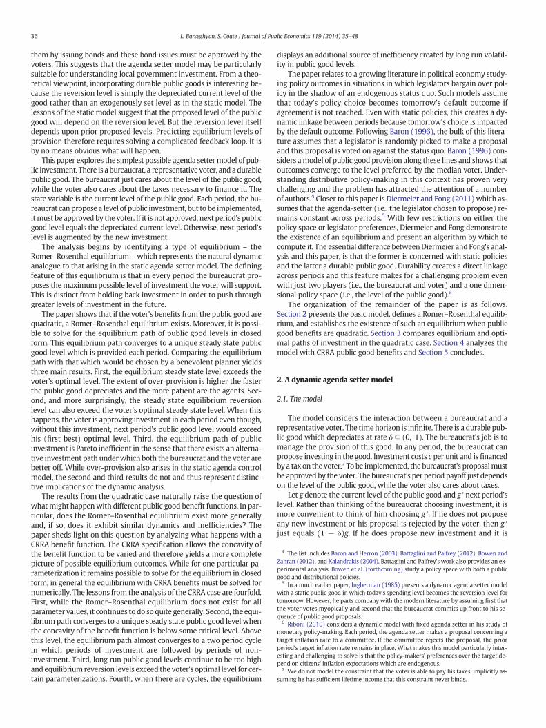
When g exceeds g∗/(1− δ) the voter will prefer the reversion level (1−δ)g to any higher level. Accordingly, the bureaucratmust simply choosethe reversion level. When g is less than g∗/(1 − δ), there exist publicgood levels higher than the reversion level that will be supported bythe voter. In a Romer–Rosenthal equilibrium, the bureaucratwill choosethe largest of these. Thismeans that hewill choose a public good level g ′(greater than (1− δ)g) such that

β V g0ð Þ−V 1−δð Þgð Þ½ � ¼ c g0− 1−δð Þgð Þ: ð5Þ

Intuitively, at this public good level, the future benefits to the voter arejust offset by the tax cost. Accordingly, we say that an equilibrium(g ′ (g), U(g), V(g)) is a Romer–Rosenthal equilibrium if g ′ (g) equals(1− δ)g if g exceeds g∗/(1− δ) and satisfies Eq. (5) otherwise.

3.1. Characterization and existence

A Romer–Rosenthal equilibrium has a very convenient property.14

Notice that when g is less than g∗/(1 − δ), Eq. (5) implies that thebureaucrat's strategy g′ (g) is such that

−c g0 gð Þ− 1−δð Þgð Þ þ βV g0 gð Þð Þ ¼ βV 1−δð Þgð Þ: ð6Þ

Substituting Eq. (6) into Eq. (3), we see that the voter's value functionsatisfies

V gð Þ ¼ B gð Þ þ βV 1−δð Þgð Þ: ð7Þ

Moreover, Eq. (7) also holds when g exceeds g∗/(1 − δ) since g ′ (g)equals (1 − δ)g. Applying Eq. (7) repeatedly, we conclude that in aRomer–Rosenthal equilibrium, the voter's value function is

V gð Þ ¼X∞t¼0

βtB 1−δð Þtg� �

: ð8Þ

Intuitively, the voter gets the same lifetime utility in equilibrium as hewould do if there were never any more investment. This reflects thefact that the bureaucrat extracts all the surplus from any new invest-ment. Note that the voter's value function is increasing and strictly con-cave as required.

When the voter has quadratic public good benefits, Eq. (8) impliesthat the voter's value function is

V gð Þ ¼ b01−β 1−δð Þ� �

g− b11−β 1−δð Þ2� �

g2: ð9Þ

Eq. (9) has some useful implications. Substituting it into Eq. (4) andsolving, we find that the voter's optimal public good level g∗ is given by:

g� ¼βb0−c 1−β 1−δð Þð Þð Þ 1−β 1−δð Þ2

� �2βb1 1−β 1−δð Þð Þ : ð10Þ

In addition, substituting Eq. (9) into Eq. (5), we can show that wheng is less than g∗/(1 − δ), the new public good level g ′ (g) is equal to2g∗ − (1 − δ)g.15 We may therefore conclude that in a Romer–Rosenthal equilibrium, the bureaucrat's strategy is given by

g0 gð Þ ¼ 2g�− 1−δð Þg if g≤g�= 1−δð Þ1−δð Þg if gNg�= 1−δð Þ :

�ð11Þ

This strategy is illustrated in Fig. 1. The current level of the publicgood g is measured on the horizontal axis and the future level g ′ onthe vertical. The dashed line is the 45° line and the flatter solid line

14 This property is also true in an equilibrium inwhich the bureaucrat holds back invest-ment, provided that whenever he does invest, he chooses the maximum possible level.15 The derivation can be found in Appendix A.

measures (1 − δ)g. The strategy g ′ (g) begins at the point (0, 2g∗),slopes down to the point (g∗/(1− δ), g∗), and thereafter follows the up-ward sloping line (1− δ)g. On the interval [0, g∗/(1− δ)] the amount ofpublic good proposed by the bureaucrat is decreasing linearly in theexisting level and the rate of decrease is just 1 − δ.

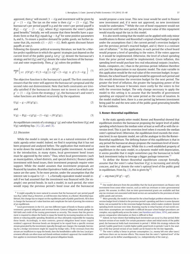
With this knowledge of the bureaucrat's strategy, the dynamic evolu-tion of the equilibriumpublic good level can be traced out. Fig. 2 illustratesthe situation. Suppose that the level of the public good at the beginning ofperiod 0 is g0. Then, in period 0, a large amount of investment takes placeand the public good level at the beginning of period 1 is g1. Since g1 ex-ceeds g∗/(1 − δ), there is no investment in period 1 and the level of thepublic good at the beginning of period 2 is g2 = (1 − δ)g1. Investmentresumes in period 2 and the level of the public good at the beginning ofperiod 3 can be obtained from the Figure in the obvious way (i.e., g3 =g ′ (g2)). Proceeding in this way, the entire future path of public goodlevels can be obtained and the bureaucrat's value function will be givenby

U g0ð Þ ¼X∞t¼0

βtgt : ð12Þ

0 gg0

g1

g2

g3

(1−δ) g

Fig. 2. Dynamics.

image of Fig.�1

image of Fig.�2

0 gg*/(1−δ)g** gs


45o line(1−δ) g

Fig. 3. Steady state.


One further step is required to establish the existence of a Romer–Rosenthal equilibrium. We need to verify that when g is less thang∗/(1 − δ), the bureaucrat is indeed better off choosing a public goodlevel g ′ that satisfies Eq. (5) rather than a smaller level. From Eq. (1),this requires showing that the bureaucrat's value function takes on avalue at g ′ (g) at least as large as the value for any g′ in the interval[(1− δ)g, g′(g)]. Intuitively, the problem is to show that the bureaucratcannot gain by holding back investment today to pass a bigger amounttomorrow. To verify this is the case, we need to compute thebureaucrat's value function from (12) and check it is maximized atg′(g).16 While in general this is a difficult problem, the simplicity ofthe bureaucrat's strategy in the quadratic case makes this possible andallows us to prove:

Proposition 1. With quadratic public good benefits, there exists a Romer–Rosenthal equilibrium with bureaucrat strategy given by Eq. (11).

Proof. See On-line Appendix B. ■

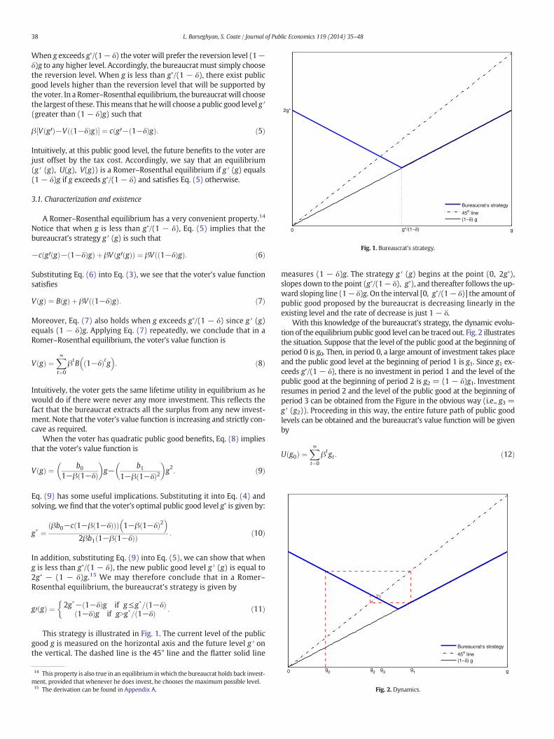
3.2. Equilibrium dynamics

The long run behavior of public good levels implied by the equilibri-um is easy to figure out. Let g∗ ∗ denote the level of public good at whichg ′ (g) equals g∗/(1 − δ). This level is illustrated in Fig. 3 and can beshown to equal g∗(1 − 2δ)/(1 − δ)2. Its significance is that if g is lessthan g∗∗, new investment is such that g ′ (g) exceeds g∗/(1 − δ) whichmeans there is no investment in the subsequent period. By contrast, if glies in the interval (g∗∗, g∗/(1 − δ)], new investment is such that g ′ (g)is less than g∗/(1 − δ) implying there is investment in the subsequentperiod. Moreover, g′ (g) exceeds g∗∗, so that there will be investment inthe following and all future periods. It follows from this that once thepublic good level enters the interval [g∗∗, g∗/(1 − δ)] it will remainthere and investment will take place each period. The public good levelwill converge with damped oscillations to the steady state level gs illus-trated in Fig. 3. At this steady state, the voters approve a constant levelof investment δgs each period.

If the public good level starts out below g∗∗, the initial period's invest-ment will put the level above g∗/(1 − δ) and a number of periods withno investment will follow until it falls below g∗/(1 − δ). After thatpoint, the level is in the interval [g∗∗, g∗/(1 − δ)] and will converge togs. If the public good level starts out above g∗/(1 − δ), a number of pe-riods with no investment will follow until it falls below g∗/(1 − δ).After that point, it will again converge to gs. The steady state levelsatisfies the equation gs = g ′ (gs) and, using Eq. (11), it is easy toshow that it is given by

gs ¼2

2−δg� ¼

βb0−c 1−β 1−δð Þð Þð Þ 1−β 1−δð Þ2� �

2−δð Þβb1 1−β 1−δð Þð Þ : ð13Þ

We have therefore proved:

Proposition 2. With quadratic public good benefits, in the Romer–Rosenthal equilibrium with bureaucrat strategy given by Eq. (11), thepublic good level converges to the steady state level gs defined inEq. (13).

16 Notice that if we had assumed the bureaucrat's per period payoff was B(g) rather thang (as discussed in footnote#8), wewould have to compute the bureaucrat's value functionfrom the equation U(g0) = ∑ t = 0

∞ βtB(gt) and check that it is maximized at g′ (g). Thisfurther complicates an already difficult task. Nonetheless, it seems intuitively that addingcurvature to the bureaucrat's per period payoff wouldmake holding back investment evenless desirable and thus would not threaten our existence result. Our numerical analysissupports this conjecture: in any case we have computed in which the Romer–Rosenthalequilibrium exists when the bureaucrat has per period payoff g it also does so when hehas per period payoff B(g).

4. Normative analysis of equilibrium

4.1. Optimal investment

We can now compare the equilibrium path of public good levelswith the path that would maximize the voter's utility. The planningproblem can be posed recursively as:

W gð Þ ¼ maxg0

B gð Þ−c g0− 1−δð Þgð Þ þ βW g0ð Þs:t: g0≥ 1−δð Þg

� �; ð14Þ

whereW(g) denotesmaximized voter welfare. Assuming the constraintin Eq. (14) is not binding, the first order condition for the optimal g ′ isthat

βW 0 g0ð Þ ¼ c: ð15Þ

Again, assuming the constraint is not binding, the Envelope Theorem im-plies that

W0 gð Þ ¼ B0 gð Þ þ c 1−δð Þ: ð16Þ

Substituting Eq. (16) into Eq. (15) and solving, we see that with qua-dratic public good benefits if the constraint is not binding, g′= gs

owhere

gos ¼βb0−c 1−β 1−δð Þð Þ

2βb1: ð17Þ

Notice that this optimal level is independent of the initial level g.17 Theinitial level matters only if it is larger than the optimal level. In that case,the constraint binds. Thus, we have that the optimal policy function is

g0 gð Þ ¼gos if g≤ gos

1−δ

1−δð Þg if gNgos

1−δ

:

8>><>>: ð18Þ

The dynamic path of public good levels generated by this policyfunction is very simple. If the initial level of the public good is lessthan gos

1−δ, then in subsequent periods the public good level is just gso.The public good level jumps to its steady state level in just one period.If the initial level exceeds gos

1−δ, there is no investment until the level of

17 Again, this reflects the fact that the voter's utility is linear in private consumption andhence there are no income effects.

image of Fig.�3


public good has fallen below gos1−δ at which time investment kicks in to

maintain the public good at its optimal level gso.

4.2. Equilibrium vs. optimal investment

We begin by comparing the equilibrium steady state gs with theoptimal steady state gs

o. Using Eqs. (17) and (13), we may write

gs−gosgos

¼ δ=2 1þ β 1−δð Þð Þ1−δ=2ð Þ 1−β 1−δð Þð Þ : ð19Þ

The left hand side of this equationmeasures the extent of over or under-provision as a fraction of the optimal level. Since the right hand side ofEq. (19) is positive, the public good is over-provided in steady state.The degree of over-provision is between 0 and 100% of the optimallevel, taking on its minimum value when δ = 0 and its maximumwhen δ = 1. Moreover, it is independent of the public good benefitand cost parameters, just depending on the agents' discount rate βand the depreciation rate δ. It can be shown to be increasing in β andδ, implying that over-provision is greater the more the agents careabout the future and the faster the public good depreciates. Thus, wehave:

Proposition 3. With quadratic public good benefits, in the Romer–Rosenthal equilibrium with bureaucrat strategy given by Eq. (11), thesteady state public good level exceeds the optimal steady state level. The de-gree of over-provision measured as a fraction of the optimal level rangesbetween 0 and 100% and depends positively on the agents' discount rateand the depreciation rate.

Proof. See Appendix A. ■

The result that themagnitude of over-provision is increasing in β re-flects the fact that the more the voter cares about the future the morepainful the prospect of having to live with the depreciated currentlevel of the public good. The positive dependence on δ reflects the factthat the faster the public good depreciates themore severe is the threatof being stuck with the depreciated current level.18 It is instructive tocompare these results concerning over-provisionwith those of the stat-ic model. When the reversion level is less than the voter's optimal level,the static model predicts that the public good will be over-provided.Moreover, with a quadratic public good benefit function, themagnitudeof over-provision as a fraction of the voter's optimal level is less than100%.19 Thus, the lessons concerning over-provision are quite similar.

These results concerning over-provision notwithstanding, there aretwo important differences between the dynamic and static models.First, a central lesson of the static model is that if the voter approvesthe bureaucrat's proposal, the reversion levelmust be belowhis optimalpublic good level. In cases where the bureaucrat passes a proposal, thereversion level therefore provides a useful lower bound estimate ofthe voter's optimal public good level. This is also true in the dynamicmodel in the sense that the equilibrium reversion level (1 − δ)gs is

18 It may seem puzzling that when the public good depreciates very slowly (small δ),there will be little difference between the equilibrium and optimal steady states. Afterall, the bureaucrat has agenda setting power and very different objectives from the voter.To understand the result, note that with small δ if the public goodwere only a little belowthe voter's optimal level the bureaucratwould be able to implement only a very small levelof investment. This is because the reversion level would differ little from the voter's opti-mal level. Since in equilibrium the bureaucrat always takes any level of investment he canget, the equilibrium level of the public goodwould therefore remain close to optimal. Nownote that, even if the community starts out with a very small level of the public good andthe bureaucrat initially implements a high level of investment, eventually depreciationmust bring the public good level down close to the optimal level.19 With quadratic public good benefits, the voter's optimal public good level in the staticmodel is (b0− c)/2b1. Themaximum level the bureaucrat can extract iswhen the reversionlevel is 0. This level satisfies b0g− b1g

2= cg, which implies that it equals (b0− c)/b1 exactlytwice the voter's optimal level. The maximum over-provision magnitude is therefore100%. This should not be surprising because when depreciation is 100% (i.e., δ = 1)the dynamic model is equivalent to the static model with a reversion level of 0.

less than the voter's optimal level g∗ (this is clear from Eq. (13)). How-ever, g∗ is the optimal level for the voter in equilibrium and it exceedsthe first best optimal level gso (compare Eq. (10) with Eq. (17)). Thismeans that it is possible that the equilibrium reversion level exceedsthe first best level. Using Eqs. (17) and (13), we can show that (1− δ)gs exceeds gso when

2 1−δð Þ þ 1ð Þβ 1−δð ÞN1: ð20Þ

Studying this inequality yields the following result:

Proposition 4. With quadratic public good benefits, in the Romer–Rosenthal equilibrium with bureaucrat strategy given by Eq. (11), for alldiscount rates β in excess of 1/3, there exists a critical value of the depreci-ation rate δ(β)∈ (0, 1) such that the equilibrium reversion level (1− δ)gsexceeds the optimal steady state level gs

o for all depreciation rates in theinterval (0, δ(β)).

Proof. See Appendix A. ■

Proposition 4 is striking in the sense that in equilibrium the voter isapproving investment in every period even though the public good levelthat would arise in the next period if the investment was not undertak-en exceeds his first best level. The intuition is that the voter values pub-lic goods more in the equilibrium because higher levels reduceexploitation by the bureaucrat.20 The lesson from this Proposition isthat the equilibrium reversion level cannot be used as a lower boundfor the first best level of public goods. This result is the most importantinsight from the model. It seems natural to assume that if voters in acommunity approve an investment, then it must be the case that thepublic good level that would prevail without the investment would be“too low”. This is correct if too lowmeans below the level that the voterswould like in equilibrium. But it is not correct if too low means belowthe first best level. This makes it hard to use bond elections to make in-ferences about political distortions in the provision of public goods.21

The second key difference between the static and dynamic modelsconcerns efficiency. In the static model, the equilibrium policy choiceis on the Pareto frontier: by construction, the equilibrium policy maxi-mizes the bureaucrat's welfare subject to a given level of utility for thevoter. In the dynamic model, however, the equilibrium path of invest-ment is Pareto inefficient. To see this, consider a modified planningproblem which puts weight λ on the citizen's payoff and 1 − λ on thebureaucrat's. The only effect of this modification is to change the opti-mal steady state to

gos λð Þ ¼ β λb0 þ 1−λð Þð Þ−λc 1−β 1−δð Þð Þλ2βb1

: ð21Þ

Now suppose that the welfare weight on the citizen is such as tomake the optimal steady state gs

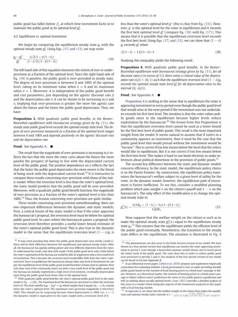
o(λ) equal to the equilibrium steadystate gs.22 This ensures that the equilibrium yields the efficient level ofthe public good eventually. Nonetheless, the transition to the steadystate differs in the equilibrium. The situation is illustrated in Fig. 4

20 This phenomenon can also occur in the finite horizon version of our model. We haveshown in a four period version that equilibrium can involve the voter approving invest-ment in period 1 even though a benevolent planner would choose not to invest giventhe initial stock of the public good. The voter does this in order to reduce public goodover-provision in periods 3 and 4. Our analysis of the four period version of our modelcan be found in On-line Appendix B.21 In an influential recent paper, Cellini et al. (2010) propose and implement empiricallya procedure for evaluatingwhether a local government is over or under providing durablepublic goods based on the reaction of local housing prices to a bond issue's passage or fail-ure. However, as a theoretical matter, the reaction of housing prices to a bond issue's pas-sage or failure reflects voters' preferences for more or less public good in equilibrium andtells us nothing about socially optimal levels. Coate (2013) provides a detailed analysis ofthis issue in a model which integrates aspects of the framework analyzed in this paperwith a local housing market.22 In Appendix A, we show that thewelfare weight on the citizen thatmakes the equilib-rium and optimal steady states coincide is λ ¼ 1−β 1−δð Þð Þβ 2−δð Þ

δ β 1−δð Þþ1ð Þ βb0−c 1−β 1−δð Þð Þð Þþ 1−β 1−δð Þð Þβ 2−δð Þ :

0 ggs g

s/(1−δ)g*/(1−δ)

Bureaucrat,s strategyOptimal policy

45o line(1−δ) g

Fig. 4. Equilibrium vs. optimum.


which compares the bureaucrat's equilibrium strategy and the optimalpolicy function under the assumption that gso(λ) equals gs. The optimalpolicy function, which comes from Eq. (18), is the dashed horizontalline.

From Fig. 4, it is clear that equilibrium exceeds optimal investmentwhenever g is less than gs and is lower whenever g lies in the intervalgs;

gs1−δð �. Thus, unless the initial level of the public good just happens to

equal gs, the equilibrium and optimal paths diverge. The over-shootingarises because the bureaucrat exploits the low reversion level byinvesting too much. The under-shooting arises because the voter ex-ploits the high reversion level by blocking efficient investment. Bothparties would be better off with an investment path that followed theoptimal rule in Eq. (18) but with a different steady state. This argumentestablishes:

Proposition 5. With quadratic public good benefits, in the Romer–Rosenthal equilibrium with bureaucrat strategy given by Eq. (11), theequilibrium path of investment is Pareto inefficient provided only that theinitial level of the public good the community begins with differs from theequilibrium steady state level.

Proposition 5 tells us that the political equilibrium exhibits politicalfailure in the sense defined by Besley and Coate (1998). The source ofthe inefficiency is lack of commitment. Starting with a low initialvalue of the public good, the voter would like to reassure the bureaucratthat he will support higher levels of investment in the future if the bu-reaucrat proposes a lower level today. However, this is not incentivecompatible. Similarly, starting with a higher initial value of the publicgood, the bureaucrat would like to reassure the voter that he will pro-pose lower levels of investment in the future if the voter supports ahigher level today. Again, this is not incentive compatible. The modeltherefore provides a nice example of political failure arising because oflack of commitment in dynamic political interactions. While far fromthe first such example, it has the virtue of emerging simply in the obvi-ous dynamic extension of a very well-known political economymodel.23

5. Beyond quadratic public good benefits

The results from the quadratic case naturally raise the question ofwhatmight happenwith different public good benefit functions. In par-ticular, does the Romer–Rosenthal equilibrium exist more generallyand, if so, does it exhibit similar dynamics and inefficiencies? This sec-tion sheds light on this question by analyzing what happens with aCRRA benefit function B(g) equal to bg1− σ/(1 − σ) where b and σ arepositive parameters.24 The CRRA specification allows the concavity ofthe benefit function to be varied (by changing σ) and therefore permitsa richer understanding of possible equilibrium outcomes than does thequadratic case.25 With this benefit function, the first best level of thepublic good is easily shown to equal

gos ¼βb

c 1−β 1−δð Þð Þ� �1

σ

: ð22Þ

23 For classic examples see Alesina and Tabellini (1990) and Persson and Svensson(1989). For other examples involving durable public investments see Battaglini and Coate(2007), Battaglini et al. (2012), Besley and Coate (1998), and Leblanc et al. (2000). In allthese examples, decision-making power fluctuates between different political actors. Inour example, by contrast, the allocation of decision-making power remains constant. Fora general discussion of commitment problems in political environments see Acemoglu(2003).24 As is standard, when σ = 1 and the CRRA benefit function is not defined, B(g) is as-sumed to take the logarithmic form b ln g.25 The CRRA function has the disadvantage of implying that the marginal benefit of thepublic good becomes infinite as its level goes to zero, which may not be a reasonable as-sumption. While this disadvantage can be overcome by adding a positive constant m tothe function so that B(g) equals (g + m)1− σ/(1 − σ), such an addition sacrifices muchof the CRRA function's famed tractability.

Given that this depends only on the ratio b/cwehenceforth set the priceof the public good c equal to 1.

As shown in Section 2.2, if a Romer–Rosenthal equilibriumexists, thevoter's value function satisfies Eq. (8). In the CRRA case, therefore, if aRomer–Rosenthal equilibrium exists, the voter's value function mustequal

V gð Þ ¼ bg1−σ

1−σ

X∞t¼0

β 1−δð Þ1−σh it

: ð23Þ

Note immediately that in order for the sum on the right hand side toconverge we require that β(1 − δ)1− σ is less than 1. If this conditionis satisfied, then the voter's value function is

V gð Þ ¼ b1−β 1−δð Þ1−σ

� �g1−σ

1−σ: ð24Þ

This function is increasing and concave as required. If the condition isnot satisfied, then the voter's value function is not defined. Thus, a nec-essary condition for the existence of a Romer–Rosenthal equilibriumwith a CRRA benefit function is that β(1− δ)1− σ is less than 1. The re-maining questions are then does a Romer–Rosenthal equilibrium existunder this condition and, if so, what are its properties? In the specialcase in which σ equals 2 these questions can be answered analytically.More generally, numerical analysis is required.

5.1. The CRRA case with σ = 2

When σ equals 2, we can prove the existence of the Romer–Rosenthal equilibrium analytically under the assumption that β is lessthan (1 − δ) and solve for the equilibrium path in closed form.Substituting Eq. (24) into (4) and solving, we find that the voter's opti-mal public good level g∗ is given by:

g� ¼ffiffiffiffiffiffiffiffiffiffiffiffiffiβb

1− β1−δ

s: ð25Þ

In addition, substituting Eq. (24) into (5), we can show that when g isless than g∗/(1 − δ), the new public good level g ′ (g) is equal to (g∗)2/

image of Fig.�4

0 g

g*/(1−δ)


45o line(1−δ) g

Fig. 5. Bureaucrat's strategy, σ = 2.

g*/(1−δ)g* g


45o line(1−δ) g

Fig. 6. Different cycles, σ = 2.


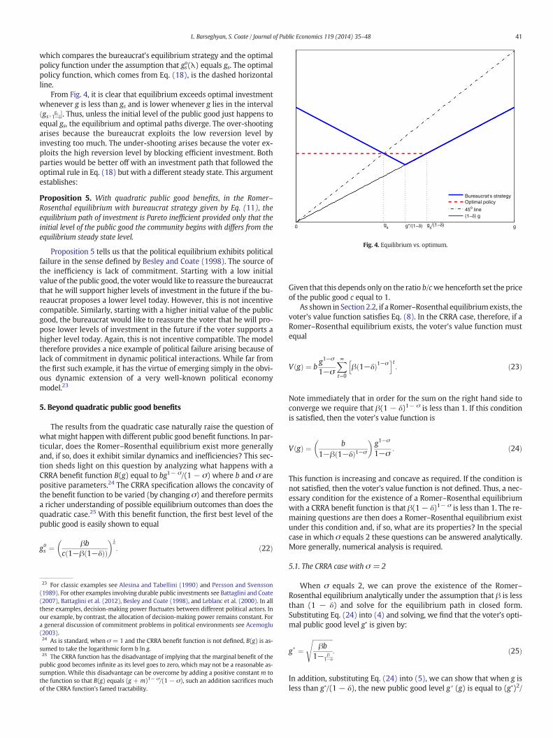
[(1 − δ)g]. 26 We may therefore conclude that in a Romer–Rosenthalequilibrium, the bureaucrat's strategy is given by

g0 gð Þ ¼g�ð Þ2

1−δð Þg if g≤g�= 1−δð Þ1−δð Þg if gNg�= 1−δð Þ

:

8<: ð26Þ

This strategy is illustrated in Fig. 5. Comparing Figs. 1 and 5, we seethat what makes this different from the quadratic case is the convexshape of the bureaucrat's strategy. The amount of public good the bu-reaucrat is able to extract from the voter increases significantly as theexisting level decreases because of the sharply increasingmarginal util-ity of the public good.27 Intuitively, this would seem to raise the incen-tive for the bureaucrat to hold back investment and thus throws intodoubt the existence of a Romer–Rosenthal equilibrium.

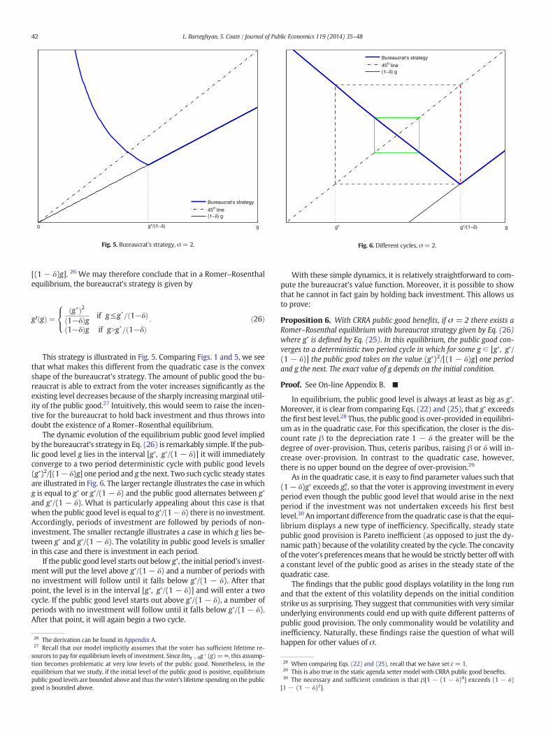
The dynamic evolution of the equilibrium public good level impliedby the bureaucrat's strategy in Eq. (26) is remarkably simple. If the pub-lic good level g lies in the interval [g∗, g∗/(1 − δ)] it will immediatelyconverge to a two period deterministic cycle with public good levels(g∗)2/[(1− δ)g] one period and g the next. Two such cyclic steady statesare illustrated in Fig. 6. The larger rectangle illustrates the case in whichg is equal to g∗ or g∗/(1 − δ) and the public good alternates between g∗

and g∗/(1 − δ). What is particularly appealing about this case is thatwhen the public good level is equal to g∗/(1− δ) there is no investment.Accordingly, periods of investment are followed by periods of non-investment. The smaller rectangle illustrates a case in which g lies be-tween g∗ and g∗/(1 − δ). The volatility in public good levels is smallerin this case and there is investment in each period.

If the public good level starts out below g∗, the initial period's invest-ment will put the level above g∗/(1 − δ) and a number of periods withno investment will follow until it falls below g∗/(1 − δ). After thatpoint, the level is in the interval [g∗, g∗/(1 − δ)] and will enter a twocycle. If the public good level starts out above g∗/(1 − δ), a number ofperiods with no investment will follow until it falls below g∗/(1 − δ).After that point, it will again begin a two cycle.

26 The derivation can be found in Appendix A.27 Recall that our model implicitly assumes that the voter has sufficient lifetime re-sources to pay for equilibrium levels of investment. Since limg ↘ 0g ′ (g) = ∞, this assump-tion becomes problematic at very low levels of the public good. Nonetheless, in theequilibrium that we study, if the initial level of the public good is positive, equilibriumpublic good levels are bounded above and thus the voter's lifetime spending on the publicgood is bounded above.

With these simple dynamics, it is relatively straightforward to com-pute the bureaucrat's value function. Moreover, it is possible to showthat he cannot in fact gain by holding back investment. This allows usto prove:

Proposition 6. With CRRA public good benefits, if σ = 2 there exists aRomer–Rosenthal equilibrium with bureaucrat strategy given by Eq. (26)where g∗ is defined by Eq. (25). In this equilibrium, the public good con-verges to a deterministic two period cycle in which for some g ∈ [g∗, g∗/(1 − δ)] the public good takes on the value (g∗)2/[(1 − δ)g] one periodand g the next. The exact value of g depends on the initial condition.

Proof. See On-line Appendix B. ■

In equilibrium, the public good level is always at least as big as g∗.Moreover, it is clear from comparing Eqs. (22) and (25), that g∗ exceedsthe first best level.28 Thus, the public good is over-provided in equilibri-um as in the quadratic case. For this specification, the closer is the dis-count rate β to the depreciation rate 1 − δ the greater will be thedegree of over-provision. Thus, ceteris paribus, raising β or δ will in-crease over-provision. In contrast to the quadratic case, however,there is no upper bound on the degree of over-provision.29

As in the quadratic case, it is easy to find parameter values such that(1− δ)g∗ exceeds gso, so that the voter is approving investment in everyperiod even though the public good level that would arise in the nextperiod if the investment was not undertaken exceeds his first bestlevel.30 An important difference from the quadratic case is that the equi-librium displays a new type of inefficiency. Specifically, steady statepublic good provision is Pareto inefficient (as opposed to just the dy-namic path) because of the volatility created by the cycle. The concavityof the voter's preferencesmeans that hewould be strictly better off witha constant level of the public good as arises in the steady state of thequadratic case.

The findings that the public good displays volatility in the long runand that the extent of this volatility depends on the initial conditionstrike us as surprising. They suggest that communities with very similarunderlying environments could end up with quite different patterns ofpublic good provision. The only commonality would be volatility andinefficiency. Naturally, these findings raise the question of what willhappen for other values of σ.

28 When comparing Eqs. (22) and (25), recall that we have set c = 1.29 This is also true in the static agenda setter model with CRRA public good benefits.30 The necessary and sufficient condition is that β[1 − (1 − δ)4] exceeds (1 − δ)[1 − (1 − δ)2].

image of Fig.�5

image of Fig.�6

0.6 0.8 1 1.2 1.4 1.6 1.8 20.5

1

1.5

2

2.5

3

g

logσ = 2σ = 3σ = 4σ = 5

45o line(1−δ)g

Fig. 7. Bureaucrat's strategies, various σ.

0.6 0.8 1 1.2 1.4 1.6 1.8 220

22

24

26

28

30

32

34

g

logσ = 2

Fig. 8. Bureaucrat's value functions, σ = 1 & 2.

32 For those readers uncomfortable with this diagrammatic argument, we have checkednumerically that the bureaucrat's value function eU gð Þ is convex.( )


5.2. The general CRRA case

We now study the model numerically for different values of σ. Weconsider values of σ in the set {1, 2, 3, 4, 5}. As a benchmark, we setthe discount rate β equal to 0.95. We are constrained in our choice ofδ by the required existence condition that β(1− δ)1− σ be less than 1.With our choice of β, this condition requires that δ is less than 0.0127when σ equals 5. Accordingly, we set δ equal to 0.0126.31

Note that as we vary σ, we will change the voter's optimal publicgood level g∗. Substituting Eq. (24) into (4) and solving, we have:

g� ¼ βb1−β 1−δð Þ1−σ

� �1σ

: ð27Þ

These changes in g∗ shift thewhole equilibrium andmakes the cases dif-ficult to compare. To circumvent this problem, as we vary σ, we will ad-just the preference parameter b to keep g∗ equal to 1. This assumptionhas the added bonus of simplifying Eq. (5) which becomes:

g0ð Þ2− 1−δð Þgð Þ1−σ

1−σ¼ g0− 1−δð Þg: ð28Þ

5.2.1. Solution procedureThe solution procedure consists of three steps. The first is to solve

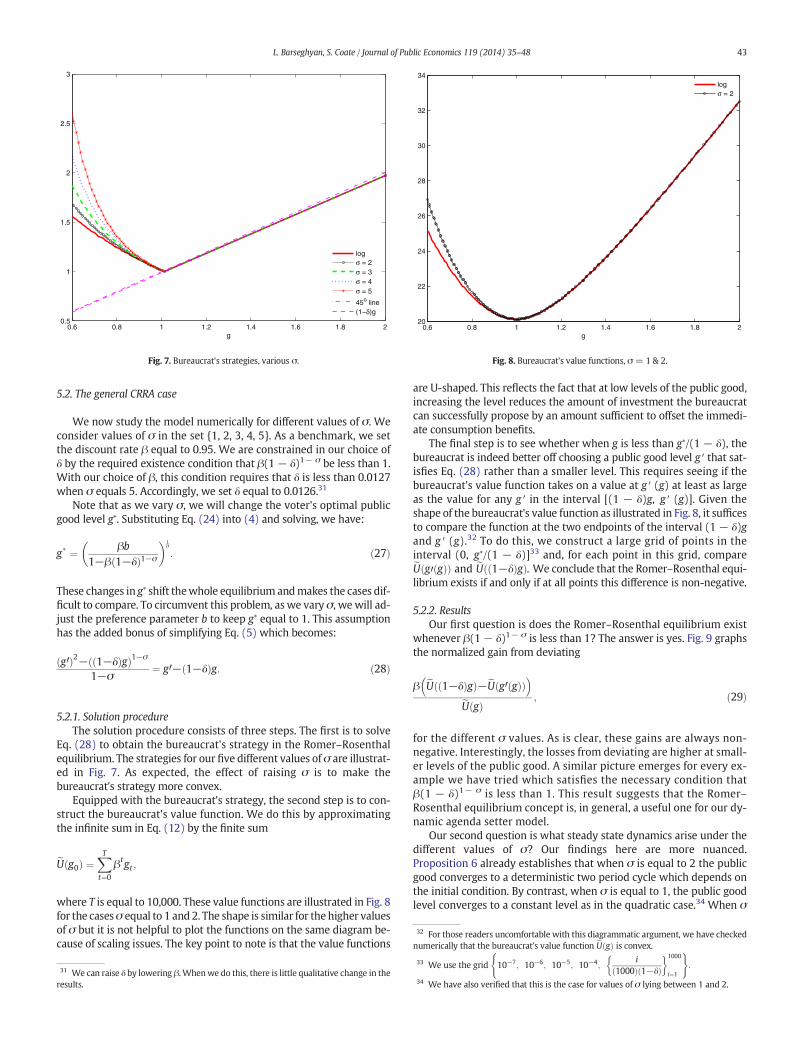
Eq. (28) to obtain the bureaucrat's strategy in the Romer–Rosenthalequilibrium. The strategies for our five different values of σ are illustrat-ed in Fig. 7. As expected, the effect of raising σ is to make thebureaucrat's strategy more convex.

Equipped with the bureaucrat's strategy, the second step is to con-struct the bureaucrat's value function. We do this by approximatingthe infinite sum in Eq. (12) by the finite sum

eU g0ð Þ ¼XTt¼0

βtgt ;

where T is equal to 10,000. These value functions are illustrated in Fig. 8for the casesσ equal to 1 and 2. The shape is similar for the higher valuesof σ but it is not helpful to plot the functions on the same diagram be-cause of scaling issues. The key point to note is that the value functions

31 We can raise δ by lowering β. Whenwe do this, there is little qualitative change in theresults.

are U-shaped. This reflects the fact that at low levels of the public good,increasing the level reduces the amount of investment the bureaucratcan successfully propose by an amount sufficient to offset the immedi-ate consumption benefits.

The final step is to see whether when g is less than g∗/(1 − δ), thebureaucrat is indeed better off choosing a public good level g ′ that sat-isfies Eq. (28) rather than a smaller level. This requires seeing if thebureaucrat's value function takes on a value at g ′ (g) at least as largeas the value for any g ′ in the interval [(1 − δ)g, g ′ (g)]. Given theshape of the bureaucrat's value function as illustrated in Fig. 8, it sufficesto compare the function at the two endpoints of the interval (1 − δ)gand g ′ (g).32 To do this, we construct a large grid of points in theinterval (0, g∗/(1 − δ)]33 and, for each point in this grid, compareeU g0 gð Þð Þ and eU 1−δð Þgð Þ. We conclude that the Romer–Rosenthal equi-librium exists if and only if at all points this difference is non-negative.

5.2.2. ResultsOur first question is does the Romer–Rosenthal equilibrium exist

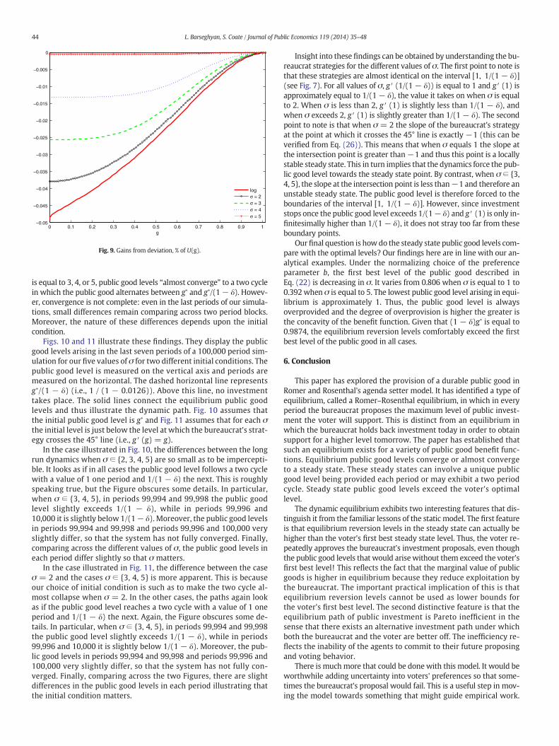
whenever β(1− δ)1− σ is less than 1? The answer is yes. Fig. 9 graphsthe normalized gain from deviating

β eU 1−δð Þgð Þ−eU g0 gð Þð Þ� �

eU gð Þ; ð29Þ

for the different σ values. As is clear, these gains are always non-negative. Interestingly, the losses from deviating are higher at small-er levels of the public good. A similar picture emerges for every ex-ample we have tried which satisfies the necessary condition thatβ(1 − δ)1− σ is less than 1. This result suggests that the Romer–Rosenthal equilibrium concept is, in general, a useful one for our dy-namic agenda setter model.

Our second question is what steady state dynamics arise under thedifferent values of σ? Our findings here are more nuanced.Proposition 6 already establishes that when σ is equal to 2 the publicgood converges to a deterministic two period cycle which depends onthe initial condition. By contrast, when σ is equal to 1, the public goodlevel converges to a constant level as in the quadratic case.34 When σ

33 We use the grid 10−7; 10−6; 10−5; 10−4;i

1000ð Þ 1−δð Þ� �1000

i¼1:

34 We have also verified that this is the case for values of σ lying between 1 and 2.

image of Fig.�7

image of Fig.�8

0 0.1 0.2 0.3 0.4 0.5 0.6 0.7 0.8 0.9 1−0.05

−0.045

−0.04

−0.035

−0.03

−0.025

−0.02

−0.015

−0.01

−0.005

0

g

logσ = 2σ = 3σ = 4σ = 5

Fig. 9. Gains from deviation, % of U(g).


is equal to 3, 4, or 5, public good levels “almost converge” to a two cyclein which the public good alternates between g∗ and g∗/(1− δ). Howev-er, convergence is not complete: even in the last periods of our simula-tions, small differences remain comparing across two period blocks.Moreover, the nature of these differences depends upon the initialcondition.

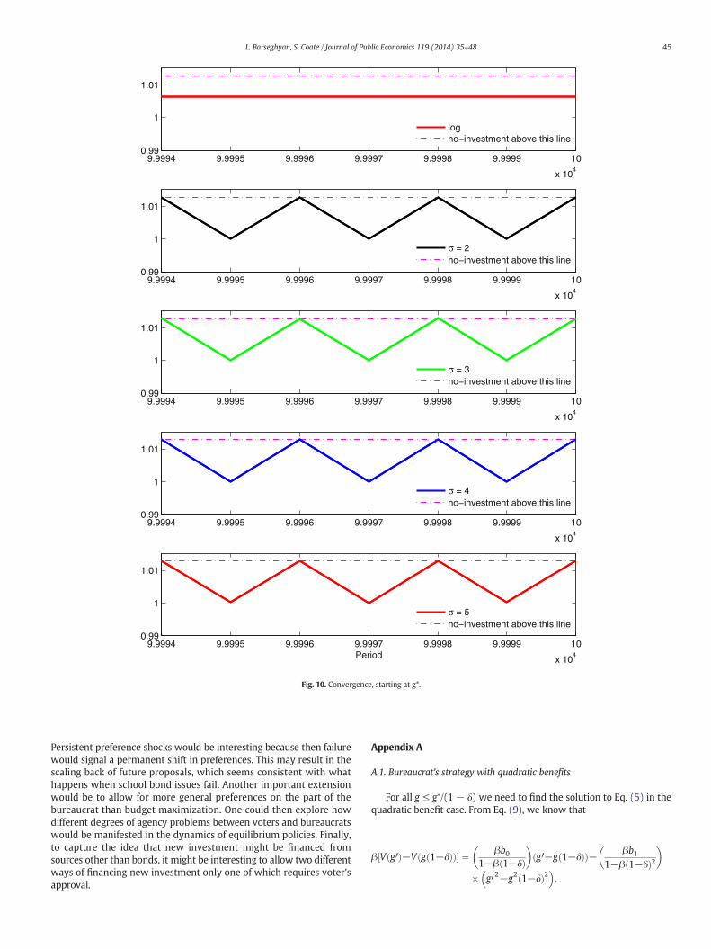
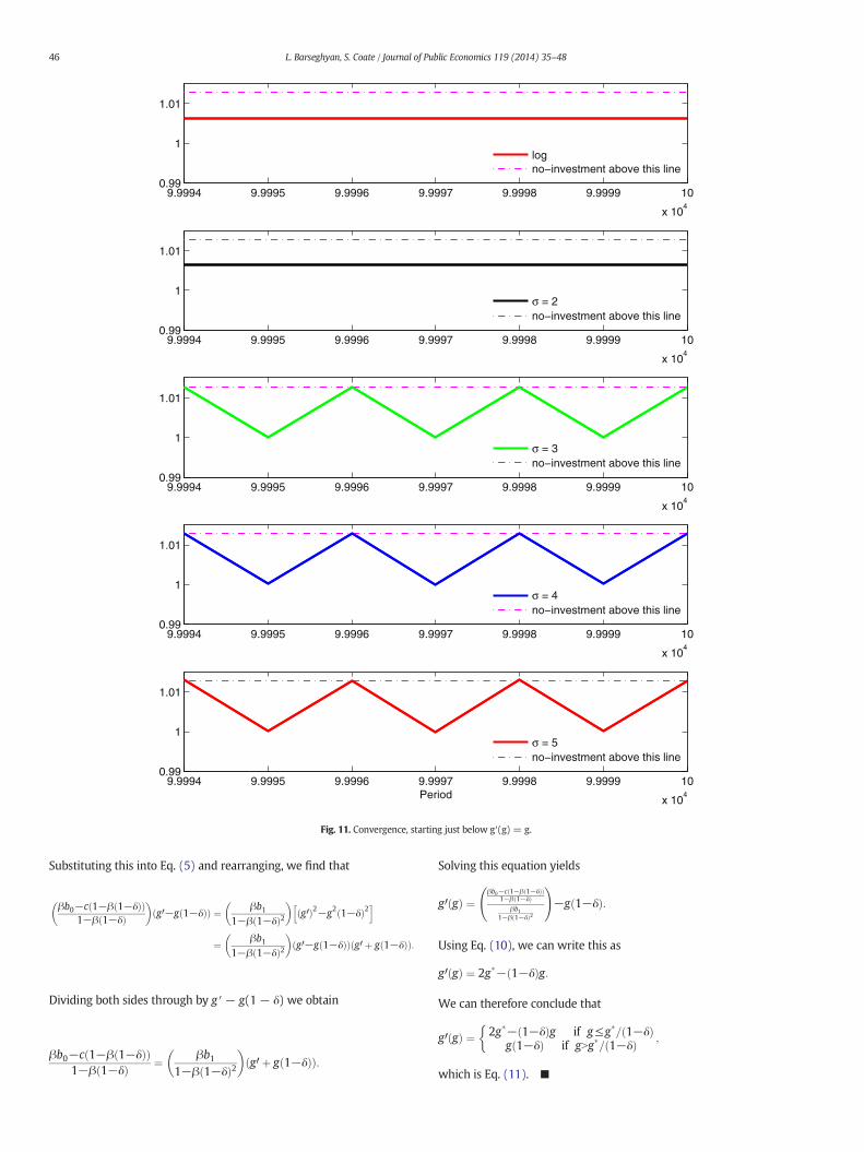
Figs. 10 and 11 illustrate these findings. They display the publicgood levels arising in the last seven periods of a 100,000 period sim-ulation for our five values of σ for two different initial conditions. Thepublic good level is measured on the vertical axis and periods aremeasured on the horizontal. The dashed horizontal line representsg∗/(1 − δ) (i.e., 1 / (1 − 0.0126)). Above this line, no investmenttakes place. The solid lines connect the equilibrium public goodlevels and thus illustrate the dynamic path. Fig. 10 assumes thatthe initial public good level is g∗ and Fig. 11 assumes that for each σthe initial level is just below the level at which the bureaucrat's strat-egy crosses the 45° line (i.e., g ′ (g) = g).

In the case illustrated in Fig. 10, the differences between the longrun dynamics when σ ∈ {2, 3, 4, 5} are so small as to be impercepti-ble. It looks as if in all cases the public good level follows a two cyclewith a value of 1 one period and 1/(1 − δ) the next. This is roughlyspeaking true, but the Figure obscures some details. In particular,when σ ∈ {3, 4, 5}, in periods 99,994 and 99,998 the public goodlevel slightly exceeds 1/(1 − δ), while in periods 99,996 and10,000 it is slightly below 1/(1− δ). Moreover, the public good levelsin periods 99,994 and 99,998 and periods 99,996 and 100,000 veryslightly differ, so that the system has not fully converged. Finally,comparing across the different values of σ, the public good levels ineach period differ slightly so that σ matters.

In the case illustrated in Fig. 11, the difference between the caseσ = 2 and the cases σ ∈ {3, 4, 5} is more apparent. This is becauseour choice of initial condition is such as to make the two cycle al-most collapse when σ = 2. In the other cases, the paths again lookas if the public good level reaches a two cycle with a value of 1 oneperiod and 1/(1 − δ) the next. Again, the Figure obscures some de-tails. In particular, when σ ∈ {3, 4, 5}, in periods 99,994 and 99,998the public good level slightly exceeds 1/(1 − δ), while in periods99,996 and 10,000 it is slightly below 1/(1 − δ). Moreover, the pub-lic good levels in periods 99,994 and 99,998 and periods 99,996 and100,000 very slightly differ, so that the system has not fully con-verged. Finally, comparing across the two Figures, there are slightdifferences in the public good levels in each period illustrating thatthe initial condition matters.

Insight into these findings can be obtained by understanding the bu-reaucrat strategies for the different values of σ. The first point to note isthat these strategies are almost identical on the interval [1, 1/(1 − δ)](see Fig. 7). For all values of σ, g′ (1/(1 − δ)) is equal to 1 and g′ (1) isapproximately equal to 1/(1− δ), the value it takes on when σ is equalto 2. When σ is less than 2, g ′ (1) is slightly less than 1/(1 − δ), andwhen σ exceeds 2, g′ (1) is slightly greater than 1/(1 − δ). The secondpoint to note is that when σ = 2 the slope of the bureaucrat's strategyat the point at which it crosses the 45° line is exactly −1 (this can beverified from Eq. (26)). This means that when σ equals 1 the slope atthe intersection point is greater than−1 and thus this point is a locallystable steady state. This in turn implies that the dynamics force the pub-lic good level towards the steady state point. By contrast, when σ ∈ {3,4, 5}, the slope at the intersection point is less than−1 and therefore anunstable steady state. The public good level is therefore forced to theboundaries of the interval [1, 1/(1 − δ)]. However, since investmentstops once the public good level exceeds 1/(1− δ) and g′ (1) is only in-finitesimally higher than 1/(1 − δ), it does not stray too far from theseboundary points.

Ourfinal question is howdo the steady state public good levels com-pare with the optimal levels? Our findings here are in line with our an-alytical examples. Under the normalizing choice of the preferenceparameter b, the first best level of the public good described inEq. (22) is decreasing in σ. It varies from 0.806 when σ is equal to 1 to0.392when σ is equal to 5. The lowest public good level arising in equi-librium is approximately 1. Thus, the public good level is alwaysoverprovided and the degree of overprovision is higher the greater isthe concavity of the benefit function. Given that (1 − δ)g∗ is equal to0.9874, the equilibrium reversion levels comfortably exceed the firstbest level of the public good in all cases.

6. Conclusion

This paper has explored the provision of a durable public good inRomer and Rosenthal's agenda setter model. It has identified a type ofequilibrium, called a Romer–Rosenthal equilibrium, in which in everyperiod the bureaucrat proposes the maximum level of public invest-ment the voter will support. This is distinct from an equilibrium inwhich the bureaucrat holds back investment today in order to obtainsupport for a higher level tomorrow. The paper has established thatsuch an equilibrium exists for a variety of public good benefit func-tions. Equilibrium public good levels converge or almost convergeto a steady state. These steady states can involve a unique publicgood level being provided each period or may exhibit a two periodcycle. Steady state public good levels exceed the voter's optimallevel.

The dynamic equilibrium exhibits two interesting features that dis-tinguish it from the familiar lessons of the static model. The first featureis that equilibrium reversion levels in the steady state can actually behigher than the voter's first best steady state level. Thus, the voter re-peatedly approves the bureaucrat's investment proposals, even thoughthe public good levels that would arise without them exceed the voter'sfirst best level! This reflects the fact that the marginal value of publicgoods is higher in equilibrium because they reduce exploitation bythe bureaucrat. The important practical implication of this is thatequilibrium reversion levels cannot be used as lower bounds forthe voter's first best level. The second distinctive feature is that theequilibrium path of public investment is Pareto inefficient in thesense that there exists an alternative investment path under whichboth the bureaucrat and the voter are better off. The inefficiency re-flects the inability of the agents to commit to their future proposingand voting behavior.

There is muchmore that could be done with this model. It would beworthwhile adding uncertainty into voters' preferences so that some-times the bureaucrat's proposal would fail. This is a useful step in mov-ing the model towards something that might guide empirical work.

image of Fig.�9

9.9994 9.9995 9.9996 9.9997 9.9998 9.9999 10

x 104

0.99

1

1.01

logno−investment above this line

9.9994 9.9995 9.9996 9.9997 9.9998 9.9999 10

x 104

0.99

1

1.01

σ = 2no−investment above this line

9.9994 9.9995 9.9996 9.9997 9.9998 9.9999 10

x 104

0.99

1

1.01


9.9994 9.9995 9.9996 9.9997 9.9998 9.9999 10

x 104

0.99

1

1.01


9.9994 9.9995 9.9996 9.9997 9.9998 9.9999 10

x 104

0.99

1

1.01

Period


Fig. 10. Convergence, starting at g*.


Persistent preference shocks would be interesting because then failurewould signal a permanent shift in preferences. This may result in thescaling back of future proposals, which seems consistent with whathappens when school bond issues fail. Another important extensionwould be to allow for more general preferences on the part of thebureaucrat than budget maximization. One could then explore howdifferent degrees of agency problems between voters and bureaucratswould be manifested in the dynamics of equilibrium policies. Finally,to capture the idea that new investment might be financed fromsources other than bonds, it might be interesting to allow two differentways of financing new investment only one of which requires voter'sapproval.

Appendix A

A.1. Bureaucrat's strategy with quadratic benefits

For all g ≤ g∗/(1 − δ) we need to find the solution to Eq. (5) in thequadratic benefit case. From Eq. (9), we know that

β V g0ð Þ−V g 1−δð Þð Þ½ � ¼ βb01−β 1−δð Þ� �

g0−g 1−δð Þð Þ− βb11−β 1−δð Þ2� �

� g02−g2 1−δð Þ2� �

:

image of Fig.�10

9.9994 9.9995 9.9996 9.9997 9.9998 9.9999 10

x 104

0.99

1

1.01

logno−investment above this line

9.9994 9.9995 9.9996 9.9997 9.9998 9.9999 10

x 104

0.99

1

1.01


9.9994 9.9995 9.9996 9.9997 9.9998 9.9999 10

x 104

0.99

1

1.01


9.9994 9.9995 9.9996 9.9997 9.9998 9.9999 10

x 104

0.99

1

1.01


9.9994 9.9995 9.9996 9.9997 9.9998 9.9999 10

x 104

0.99

1

1.01

Period


Fig. 11. Convergence, starting just below g′(g) = g.


Substituting this into Eq. (5) and rearranging, we find that

βb0−c 1−β 1−δð Þð Þ1−β 1−δð Þ

� �g0−g 1−δð Þð Þ ¼ βb1

1−β 1−δð Þ2� �h

g0ð Þ2−g2 1−δð Þ2i

¼ βb11−β 1−δð Þ2� �

g0−g 1−δð Þð Þ g0 þ g 1−δð Þð Þ:

Dividing both sides through by g ′ − g(1− δ) we obtain

βb0−c 1−β 1−δð Þð Þ1−β 1−δð Þ ¼ βb1

1−β 1−δð Þ2� �

g0 þ g 1−δð Þð Þ:

Solving this equation yields

g0 gð Þ ¼βb0−c 1−β 1−δð Þð Þ

1−β 1−δð Þβb1

1−β 1−δð Þ2

!−g 1−δð Þ:

Using Eq. (10), we can write this as

g0 gð Þ ¼ 2g�− 1−δð Þg:

We can therefore conclude that

g0 gð Þ ¼ 2g�− 1−δð Þg if g≤g�= 1−δð Þg 1−δð Þ if gNg�= 1−δð Þ ;

�which is Eq. (11). ■

image of Fig.�11


A.2. Proof of Proposition 3

Given the discussion in the text, it suffices to show that the over-provision magnitude in Eq. (19) is increasing in β and δ. The over-provision magnitude is

δ=2 1þ β 1−δð Þð Þ1−δ=2ð Þ 1−β 1−δð Þð Þ :

It is clear from inspection that this is increasing in β. Differentiatingwithrespect to δ, we obtain

∂ δ=2 1þβ 1−δð Þð Þ1−δ=2ð Þ 1−β 1−δð Þð Þ

� �∂δ ¼ 2 1−βð Þ

2−δð Þ 1−β 1−δð Þð Þ½ �2:

This is positive as required. ■

A.3. Proof of Proposition 4

The equilibrium reversion level is (1− δ)gs and the first best level isgso. We first show that (1 − δ)gs exceeds gso when Eq. (20) is satisfied.

Using Eqs. (17) and (13), we see that the equilibrium and optimalsteady states are related by the following equation

gs ¼ gos1−β 1−δð Þ2

1−δ=2ð Þ 1−β 1−δð Þð Þ

!:

It follows that

1−δð Þgs ¼ gos1−δð Þ 1−β 1−δð Þ2

� �1−δ=2ð Þ 1−β 1−δð Þð Þ

0@ 1A:

Thus, (1− δ)gs exceeds gso when

1−δð Þ 1−β 1−δð Þ2� �

N 1−δ=2ð Þ 1−β 1−δð Þð Þ

or equivalently when

1−δð Þ 1−β 1−δð Þ2� �

N 1−δð Þ 1−β 1−δð Þð Þ þ δ=2 1−β 1−δð Þð Þ:

This in turn is equivalent to

1−δð Þ β 1−δð Þδð ÞNδ=2 1−β 1−δð Þð Þ

which simplifies to

2 1−δð Þ þ 1½ �β 1−δð ÞN1;

as required.We next show that for all β N 1/3, there exists δ(β)∈ (0, 1) such that

Eq. (20) is satisfiedwhenever δ∈ (0, δ(β)). For givenβ, define the func-tion

φβ δð Þ ¼ 2 1−δð Þ þ 1ð Þβ 1−δð Þ−1:

Clearly, Eq. (20) is satisfied whenever φβ(δ) N 0. Observe first that

φβ 0ð Þ ¼ 3β−1N0N−1 ¼ φβ 1ð Þ;

where the first inequality follows from the assumption that β N 1/3.Next observe by inspection that φβ(δ) is decreasing. By continuity,there exists a unique δ(β) ∈ (0, 1) such that φβ(δ(β)) = 0. It followsthat φβ(δ) N 0 for all δ ∈ (0, δ(β)). The result follows. ■

A.4. Equilibrium welfare weight

Using Eqs. (13) and (21), we see that the welfare weight on the cit-izen that makes the optimal steady state gs

o(λ) equal to the equilibriumsteady state gs satisfies the equation

βb0−c 1−β 1−δð Þð Þð Þ 1−β 1−δð Þ2� �

2−δð Þβb1 1−β 1−δð Þð Þ ¼ β λb0 þ 1−λð Þð Þ−λc 1−β 1−δð Þð Þλ2βb1

:

Solving this for λ implies that

λ ¼ β 2−δð Þ 1−β 1−δð Þð Þ2 βb0−c 1−β 1−δð Þð Þð Þ 1−β 1−δð Þ2

� �þ 2−δð Þ 1−β 1−δð Þð Þc 1−β 1−δð Þð Þ þ 2−δð Þ 1−β 1−δð Þð Þβ 1−b0ð Þ

" # :

Collecting terms in the denominator, we can write this more simply as

λ ¼ β 2−δð Þ 1−β 1−δð Þð Þδ β 1−δð Þ þ 1ð Þ βb0−c 1−β 1−δð Þð Þð Þ þ β 2−δð Þ 1−β 1−δð Þð Þ ;

which is the expression in footnote 20. ■

A.5. Bureaucrat's strategy with CRRA benefits when σ = 2

When σ = 2, Eq. (24) tells us that the voter's value function is

V gð Þ ¼ − bg 1− β

1−δð Þ :

From Eq. (6) when g is less than g∗/(1 − δ), the strategy g ′ (g) is suchthat

− g0 gð Þ− 1−δð Þgð Þ− βbg0 gð Þ 1− β

1−δð Þ ¼ − βb1−δð Þg 1− β

1−δð Þ :

Multiplying through by g ′ (g) and rearranging yield the following qua-dratic equation

g0 gð Þ2−g0 gð Þ 1−δð Þg þ βb1−δð Þg 1− β

1−δð Þ

þ βb1− β

1−δð Þ ¼ 0:

This has solution

g0 gð Þ ¼ βb1−δð Þg 1− β

1−δð Þ ¼g�� 21−δð Þg;

which implies Eq. (26).

Appendix B. Supplementary data

Supplementary data to this article can be found online at http://dx.doi.org/10.1016/j.jpubeco.2014.07.009.

References

Acemoglu, Daron, 2003. Why not a political coase theorem? Social conflict, commitmentand politics. J. Comp. Econ. 31, 620–652.

Alesina, Alberto,Tabellini, Guido, 1990. A positive theory of fiscal deficits and governmentdebt. Rev. Econ. Stud. 57, 403–414.

Baron, David, 1996. A dynamic theory of collective goods programs. Am. Pol. Sci. Rev. 90,316–330.

Baron, David,Herron, Michael, 2003. A dynamic model of multidimensional collectivechoice. In: Kollman, Ken, Miller, John, Page, Scott (Eds.), Computational Models inPolitical Economy. MIT Press, Cambridge, MA.

Battaglini, Marco, Coate, Stephen, 2007. Inefficiency in legislative policy-making: adynamic analysis. Am. Econ. Rev. 97, 118–149.

Battaglini, Marco,Palfrey, Thomas, 2012. The dynamics of distributive politics. EconomicTheory 49, 739–777.

Battaglini, Marco,Nunnari, Salvatore,Palfrey, Thomas, 2012. Legislative bargaining and thedynamics of public investment. Am. Pol. Sci. Rev. 106, 407–429.



http://refhub.elsevier.com/S0047-2727(14)00173-X/rf0005
















Bergstrom, Ted, 1979. When does majority rule supply public goods efficiently? Scand. J.Econ. 81, 216–226.

Besley, Timothy,Coate, Stephen, 1998. Sources of inefficiency in a representative democracy:a dynamic analysis. Am. Econ. Rev. 88, 139–156.

Bowen, Howard, 1943. The interpretation of voting in the allocation of economicresources. Q. J. Econ. 58, 27–48.

Bowen, Renee, Zahran, Zaki, 2012. On dynamic compromise. Games Econ. Behav. 76,391–419.

Bowen,Renee,Chen,Ying,Hulya Eraslan, 2014. Mandatory versus discretionary spending:the status quo effect. Am. Econ. Rev. forthcoming.

Cellini, Stephanie, Ferreira, Fernando,Rothstein, Jesse, 2010. The value of school facilityinvestments: evidence from a dynamic discontinuity design. Q. J. Econ. 125, 215–261.

Coate, Stephen, 2013. Evaluating durable public good provision using housing prices, un-published manuscript.

Diermeier, Daniel, Fong, Pohan, 2011. Legislative bargaining with reconsideration. Q. J.Econ. 126, 947–985.

Hamilton, Howard,Cohen, Sylvan, 1974. Policy Making by Plebiscite: School Referenda.Lexington Books, Lexington, MA.

Ingberman, Daniel, 1985. Running against the status quo: institutions for direct democracyreferenda and allocations over time. Public Choice 46, 19–43.

Kalandrakis, Anastassios, 2004. A three-player dynamic majoritarian bargaininggame. J. Econ. Theory 116, 294–322.

Leblanc, William,Snyder, James,Tripathi, Mickey, 2000. Majority-rule bargaining and theunder provision of public investment goods. J. Public Econ. 75, 21–47.

Lizzeri, Alessandro,Persico, Nicola, 2001. The provision of public goods under alternativeelectoral incentives. Am. Econ. Rev. 91, 225–239.

Lizzeri, Alessandro,Persico, Nicola, 2005. A drawback of electoral competition. J. Eur. Econ.Assoc. 3, 1318–1348.

Niskanen, William, 1971. Bureaucracy and Representative Government. Aldine-Atherton,Chicago.

Persson, Torsten,Svensson, Lars, 1989. Why a stubborn conservative would run a deficit:policy with time-inconsistent preferences. Q. J. Econ. 104, 325–345.

Riboni, Alessandro, 2010. Committees as substitutes for commitment. Int. Econ. Rev. 51,213–236.

Romer, Thomas, Rosenthal, Howard, 1978. Political resource allocation, controlledagendas, and the status quo. Public Choice 33, 27–43.

Romer, Thomas,Rosenthal, Howard, 1979a. The elusive median voter. J. Public Econ. 12,143–170.

Romer, Thomas,Rosenthal, Howard, 1979b. Bureaucrats versus voters: on the politicaleconomy of resource allocation by direct democracy. Q. J. Econ. 93, 563–587.

Romer, Thomas,Rosenthal, Howard, 1982. Median voters or budgetmaximizers: evidencefrom school expenditure referenda. Econ. Inq. 20, 556–578.

Romer, Thomas,Rosenthal, Howard,Munley, Vincent, 1992. Economic incentives andpolitical institutions: spending and voting in school budget referenda. J. PublicEcon. 49, 1–33.

Volden, Craig,Wiseman, Alan, 2007. Bargaining in legislatures over particularistic and col-lective goods. Am. Pol. Sci. Rev. 101, 79–92.














































Documents

Bureaucrats, voters, and public investment