Bulletin of the Seismological Society of America, Vol. 74, No. 2, pp. 479-492, April 1984

RAPID SEISMIC RAY TRACING IN A SPHERICALLY SYMMETRIC EARTH VIA INTERPOLATION OF RAYS

BY ROBERT P. COMER

ABSTRACT

From the equations for seismic ray tracing in a general three-dimensionally heterogeneous isotropic elastic medium, we derive equations appropriate for a spherically symmetric earth, with path length as the independent parameter. Numerical integration of these equations, plus their derivatives with respect to take-off angle, leads to a set of reference rays for the direct P phase. From a modest number of reference rays, which need be computed only once for a given earth model, ray path coordinates and travel times can be rapidly and accurately computed by Hermite cubic interpolation using specific algorithms which we outline. Because of the speed of the interpolation and the explicit parameteriza- tion in terms of path length, this technique is ideally suited for use in a tomo- graphic inversion of global P-wave travel-time observations to obtain an estimate of lateral velocity heterogeneity in the mantle.

I N T R O D U C T I O N

A principal goal of the present work is to permit an economical tomographic inversion of global P-wave travel times for mantle heterogeneity. Seismic tomog- raphy (Clayton and Hearn, 1982; Clayton, in preparation, 1984) constructs images of slowness anomalies in the earth by back-projecting travel-time residuals along ray paths. The essential characteristic of the tomographic back-projection is a compositing of each residual into the model cells intersected by its corresponding ray. A global application of tomography requires that for each of over 106 rays, a travel time be calculated and ray path coordinates be determined along the ray, at equal intervals in path length, in an efficient manner. For this purpose, we have developed a new method for ray tracing calculations in a spherically symmetric earth and a method for interpolating between rays, which is much faster than tracing every ray.

First, we note the well-known fact (Julian and Anderson, 1968; Aki and Richards, 1980; Lee and Stewart, 1981; Thurber, 1981) that the perturbation in travel time t along a seismic ray due to a slight perturbation in the velocity model is

where s is path length, v denotes the velocity structure, and the integration is performed along the unperturbed ray path. As Buland (1982) remarked in connec- tion with the problem of earthquake location in a spherical earth with slight lateral heterogeneity, the ray path used to calculate 5t via (1) may be obtained using a spherically symmetric earth model. In the tomography problem this approximation also holds, which results in a great simplification from the formidable task of tracing so many rays in a three-dimensionally heterogeneous earth.

The calculation of travel time and angular distance A for a ray in a spherically symmetric earth is a classic problem in seismology and has, of course, been studied intensively in the past. The traditional approach involves using integral expressions

479

480 ROBERT P. COMER

for t and A where the radius from the center of the earth r or some abstract function of r and v(r) is used as the variable of integration (e.g., Bullen, 1963; Buland, 1982). However, as the form of (1) shows, in tomography and related problems, parame- terization of the ray path in terms of the path length s is highly desirable, if not essential. Traditional methods can provide such a parameterization only in an indirect and inefficient fashion. So, instead of extending classical methods, in this paper we solve the problem of seismic ray tracing in a spherically symmetric earth by a method originally developed for ray tracing in general three-dimensionally heterogeneous isotropic media.

In most approaches to three-dimensional seismic ray tracing, systems of simul- taneous differential equations are solved numerically using either t (e.g., Julian, 1970) or s (e.g., Jacob, 1970; Pereyra et al., 1980; Comer and Aki, 1981) as the independent parameter. In the next two sections, we derive a convenient form of the equations for three-dimensional ray tracing in spherical coordinates parameter- ized in terms of s, then simplify these for the special case of spherical symmetry. The resulting equations have previously appeared in somewhat fragmentary form (e.g., Bullen, 1963), but have never been grouped as a single system to be solved simultaneously by integration over s. Hence, while our novel derivation is not strictly necessary, it helps to emphasize that our method of solution of the ray equations in spherical symmetry is more akin to those applied to three-dimensional ray tracing than to the classical formulation.

In addition to the ray tracing method, this paper presents the new concept of interpolation between rays. We develop a method by which the radius from the earth's center r and angular distance A may be computed for the endpoint of a ray given its take-off angle at the earth's surface i and its path length s, by interpolation on a system of reference rays. It has been applied successfully for direct P waves in a Jeffreys-Bullen earth model for A _--_ 25 °. This range in A avoids the triplications in the P travel-time curve due to the upper mantle gradients and discontinuities, and assures a one-to-one mapping between the spaces (r, A) and (i, s). The mapping can be readily performed in either direction and the travel-time t may also be accurately and quickly calculated by an interpolation method. The Jeffreys-Bullen model is used here because for earthquake location and travel-time residual calcu- lation the ISC uses the Jeffreys-Bullen tables (e.g., Bulletin of the ISC, 1971-1980).

It is helpful to relate the present work to the two standard problems in ray tracing. These are the initial value problem {e.g., Julian, 1970; Jacob, 1970; Comer and Aki, 1981), in which the initial ray position and direction are given, and the two-point boundary value problem (e.g., Yang and Lee, 1976; Julian and Gubbins, 1977; Pereyra et al., 1980), in which a ray must be found that connects two specified points. The latter problem is more time consuming, since it must usually be solved iteratively, but a solution is needed for most practical applications, including tomography. An advantage of ray interpolation is that in ray tracing to set up the reference ray set it is necessary to solve only the initial value problem. The two- point problem then is handled easily by interpolation on the reference rays.

RAY EQUATIONS

The differential equations governing seismic rays in an elastic, isotropic, three- dimensionally heterogeneous medium are given by

ds = V

RAPID RAY TRACING VIA INTERPOLATION 481

where £(s) is the position vector, s is the path length, and v(2) is the velocity field. Note that this expression is independent of any particular coordinate system. The derivation of these equations from either the eikonal equation or Fermat's principle may be found in a variety of sources, including Aki and Richards (1980) and Lee and Stewart (1981). Introducing the slowness vector/5 = (l/v) d£/ds (e.g., Julian, 1970; Cerven~ et al., 1977), we have the first order differential equations

d~ ds v~ (2a)

Next, we obtain the scalar equations corresponding to (2) for spherical coordinates (r, 0, ¢) where r is radial distance, 0 is colatitude, and ¢ is longitude. In terms of unit vectors ~, 0, and ~,

d,2 = ?dr + OrdO + ~ r sin 0 d~

1 Ov OOv + _ _ .

V = - ~ l"-~r + rO----O r s i n O

Using these relations and the nonzero derivatives of the unit vectors,

O? ~ O? ~ sin 0 O0 O~

og_ ~ __Og=~cos0 O0 O~

o~ = - ~ sin 0 - 0 cos 0

it follows from (2a) that

dr ds vpr

dO v - - P o

ds r

d~ v ds r sin 0

(3a)

482 ROBERT P. COMER

and from (2b) that

dpr ds

v 1 0 v - r ( p ° 2 + p 2 ) _ v ~ 0~

dpo v 1 0 v ds - r (prpo - cot 0 p~,2) v2r O0

dp~ v 1 Ov ds - r (PrP~' + cot 0 PoP~') (3b)

v2r sin 0 0~"

Although they are very different in appearance, (3) and the system of ray equations in spherical coordinates derived by Jacob (1970) are exactly equivalent. Using ds =

v dr, where t denotes the travel time, the equivalence of (3) to the formulation by Julian (1970) also can be established. One can, of course, calculate t by solving simultaneously with (3) the additional equation

d t 1 - ( 4 )

ds v"

This was likewise added by Pereyra et al. (1980) to their system of ray equations, in which Cartesian coordinates are used but, as in (3), s is taken as the independent parameter.

It is helpful to note that (3b) may be recast in the somewhat simpler form

d 1 r Ov

ds [rpr] = v v 2 Or

d 1 0 v ds [rpo] = v cot 0 po 2 v ~ O0

d 1 Ov ds [rp~] = - v cot 0 pop~ v 2 sin 0 0~ (5)

which is especially convenient for introducing spherical symmetry. In the spherically symmetric case, Ov/O0 = 0 and Ov/O~ = 0, and we may rotate

the coordinates so that ~ is constant and p~ = 0. If we also let q = rpr and p = rp,

and, to emphasize the special geometry of the problem, replace 0 by A, then (3a) and (5) become

dr vq

ds r

d A vp

ds r 2

dq 1 r dv

ds v v 2 dr

@ ds

- 0 (6)

RAPID RAY TRACING VIA INTERPOLATION 483

where v now depends only on r. It is clear from (6) that p is constant on a given ray; it is in fact the classical ray parameter (Bullen, 1963), and the first two equations in (6) also have been given by Bullen, but in slightly different forms.

DYNAMIC RAY EQUATIONS FOR SPHERICAL SYMMETRY

When using a ray method to calculate dynamic quantities such as seismic waveforms and amplitudes, in addition to kinematic quantities such as ray coordi- nates, direction, and travel time, additional equations must be solved along with the ordinary ray equations. These can give information on the geometric spreading, for example, but in the present case we introduce additional equations to permit more accurate interpolation between rays. The interpolation method which will be described in the next section uses path length s and take-off angle i as independent variables from which radius r and angular distance A may be obtained via interpo- lation on a set of reference rays. Hence, in tracing a given ray, it will be useful to calculate derivatives of the coordinates with respect to i. (One could just as easily use p and s rather than i and s to parameterize the system of rays. The latter has no advantage except for its straightfoward geometrical meaning.)

Considering a ray taking off from the earth's surface (r = re), we define ri = Or~ Oi, Ai = OA/Oi, qi = Oq/ai, and Pi = Op/ai. p and pi are both constant along the ray and

p = re sin i/v(re)

Pi = re cos i/v(re).

Then, from (4), (6), and the derivative of (6) with respect to i, we have the dynamic ray equations

dr vq

ds r

d A vp

ds r 2

dq = 1 ~I ds v \

dri qv ds r 2

dAi _ pv d s r 3

dqi [ 2

ds - - Y

dt 1

( 1 - - + - qi v r

( r ;r) v 2 - - ri + Pi v V

dv ( r d v ) r d2v l d r 1 - - + v ri

- (7) ds v

ROBERT P. COMER

r(O) = re ri(O) = 0

~(o) = o ~ ( o ) = o

q(O) = - p i qi(O) = p

t ( 0 ) = 0.

v e l o c i t y , km/s 5 6 7 8 9 10 11 12 13 14

I I I I I I I I I i

(8)

(:3 0 O ,

E

r"

O. 0

23 o o o , fO

o o (C,, O0

484

wi th the init ial cond i t ions

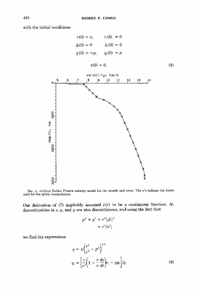
FIG. 1. Jeffreys-Bullen P-wave velocity model for the mantle and crust. The x's indicate the knots used for the spline interpolation.

Our der iva t ion o f (7) impl ic i t ly a s s u m e d v ( r ) to be a con t inuous funct ion . At d iscont inui t ies in v, q, a nd qi are also d i scont inuous , and us ing the fac t t h a t

p2 + q2 = r2[ /5[2

--_ r2 /v 2,

we f ind the express ions

r \ 1 / 2 q = 4- ~ - p2/]

~- - - - r i - - P P i / q q i v

(9)

RAPID RAY TRACING VIA INTERPOLATION 485

which enable one to continue the ray across abrupt changes in v. Note that q < 0 for downgoing rays and q > 0 for upgoing rays.

A program has been developed to solve (7) and (8) for direct P-wave ray paths in a Jeffreys-Bullen earth model. The P-wave velocity function, which is illustrated in Figure 1, is interpolated using the cubic spline FORTRAN subroutine SPLINE, by Forsythe et al. (1977), giving continuous values of v, dv/dr, and d2v/dr 2, except at the Mohorovi~i6 discontinuity. For the portions of ray path that are in the mantle, (7) is integrated using the FORTRAN subroutine DEROOT by Shampine and Gordon (1975), (9) is applied at the Moho crossings, and in the constant velocity crust an analytic solution to (7), which is given in the Appendix, is used. DEROOT

f FIG. 2. Rays for direct P from a surface source traced through the Jeffreys-Bullen earth model. Here,

and in Figures 4 and 6, the large and small concentric arcs represent the earth's surface and the core- mantle boundary, respectively.

is a predictor-corrector routine designed for general systems of simultaneous non- linear first-order differential equations. It has been previously applied to ray tracing problems by F. Luk and W. H. K. Lee (unpublished data, 1979), and Comer and Aki (1981). A sample of ray paths calculated with the program is shown in Fig- ure 2.

As the ray tracing program steps along in s, for a given value of i, the following quantities are saved for later use: s, t, q, r, Or/Oi, Or/Os, 02r/Oic)s, A, OA/c)i, OA/Os, and 02A/OiOs. In solving (7) for a given ray, i is held constant and the derivatives with respect to s are full derivatives, but for a system of rays with a common starting point, r and A are functions of both i and s. A second program has been developed that can solve several ray tracing problems by interpolating on the output produced by the first program for a set of "reference rays."

486 ROBERT P. COMER

INTERPOLATION FOR COORDINATES

For direct P waves with surface to surface angular distances of greater than about 25 °, beyond the upper mantle triplications, there is a one-to-one mapping of (i, s) to (r, A). Thus, given an arbitrary pair of i and s values, it is possible to estimate the corresponding r and A values, and travel-time t by interpolating between points on rays that are close neighbors of the arbitrary point. In this section, we describe only the interpolation for r and A.

The basic technique used is Hermite cubic interpolation (Dahlquist and Bjorck, 1974). Given a single-valued function of a single variable whose value and first derivative are known at the end points of some interval, there is a unique cubic polynomial on that interval which matches the values and derivatives at the end points. Cubics fit to the adjacent intervals formed by a set of knots at which function values and first derivatives are known will form a continuous interpolating function

S

/

r

(b)

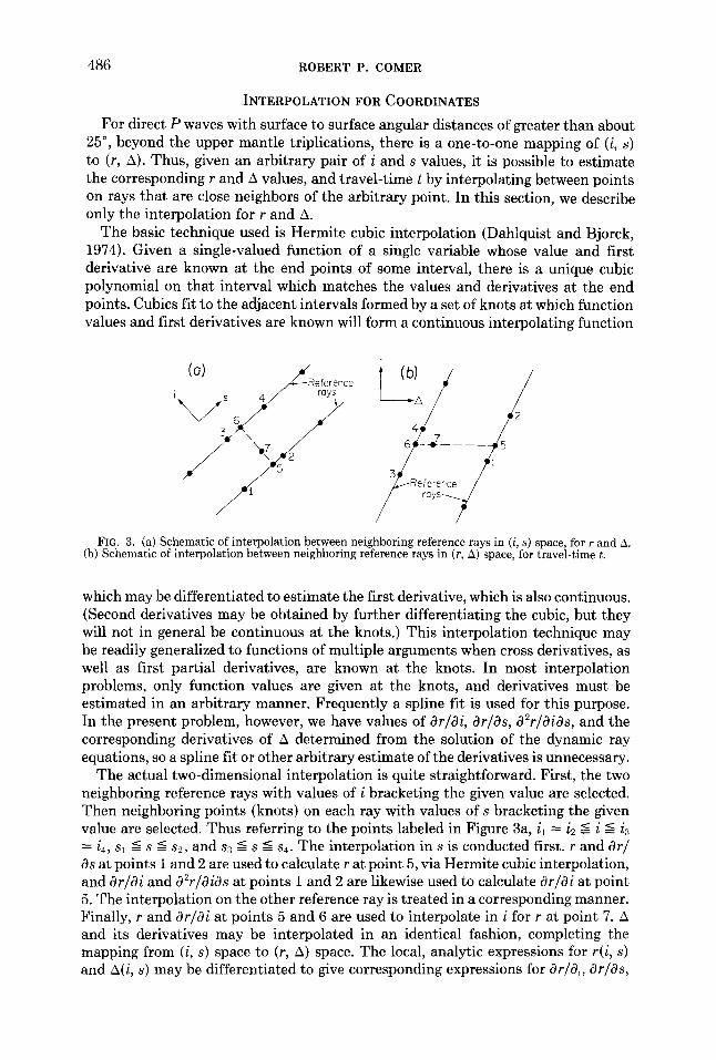
~Reference ~ raysv FI6. 3. (a) Schematic of interpolation between neighboring reference rays in (i, s) space, for r and A.

(b) Schematic of interpolation between neighboring reference rays in (r, A) space, for travel-time t.

which may be differentiated to estimate the first derivative, which is also continuous. (Second derivatives may be obtained by further differentiating the cubic, but they will not in general be continuous at the knots.) This interpolation technique may be readily generalized to functions of multiple arguments when cross derivatives, as well as first partial derivatives, are known at the knots. In most interpolation problems, only function values are given at the knots, and derivatives must be estimated in an arbitrary manner. Frequently a spline fit is used for this purpose. In the present problem, however, we have values of c)r/Oi, c)r/Os, 82r/OiOs, and the corresponding derivatives of A determined from the solution of the dynamic ray equations, so a spline fit or other arbitrary estimate of the derivatives is unnecessary.

The actual two-dimensional interpolation is quite straightforward. First, the two neighboring reference rays with values of i bracketing the given value are selected. Then neighboring points (knots) on each ray with values of s bracketing the given value are selected. Thus referring to the points labeled in Figure 3a, il = i2 -- i -< i3 = i4, sl =< s = s2, and s3 -<- s =< s4. The interpolation in s is conducted first, r and Or~ 0s at points 1 and 2 are used to calculate r at point 5, via Hermite cubic interpolation, and c)r/c)i and c)2r/Oias at points 1 and 2 are likewise used to calculate Or/Oi at point 5. The interpolation on the other reference ray is treated in a corresponding manner. Finally, r and ar/Oi at points 5 and 6 are used to interpolate in i for r at point 7. A and its derivatives may be interpolated in an identical fashion, completing the mapping from (i, s) space to (r, A) space. The local, analytic expressions for r(i, s) and A(i, s) may be differentiated to give corresponding expressions for Or/Oi, Or/Os,

RAPID RAY TRACING VIA INTERPOLATION 487

OA/Oi, and OA/Os. We note that special care must be taken near discontinuities in v to ensure reliable interpolation. Each time a reference ray crosses the Moho, two values of q and the derivatives of r and A are stored for interpolation on each side Of the discontinuity.

In practical problems, i and s are rarely known a priori. One is more likely to be given a pair of earthquake and station locations and to desire information about the ray path connecting them. For a station on the surface and a source at some depth, it is most convenient to consider the ray to start at the station and end at the source. Then, knowing A and setting r to a value appropriate to the earthquake depth, the first problem is to invert the mapping defined above to obtain i and s. Once this inversion is accomplished, it is straightforward to find points on the ray path at whatever spacing in path length is desired, by using the forward mapping.

The inverse mapping is accomplished by an iterative procedure. Given the target point (r', A'), an initial guess of (i, s) is made, based on approximate linear formulas for p and s in terms of A for a surface source (see Figure 5). Then Newton's method is applied, with r, Or/Oi, Or/c)s, A, aA/Oi, and OA/Os being calculated from in and sn at the nth iteration and the matrix equation

[ O r / O i O r / O s l [ i ' + l - is,] = [A', -- rA] (10) OA/Oi OA/Osj[sn+l

being solved by Gauss elimination. [In regions where the mapping is one-to-one, the matrix in (10) is always nonsingular and may be inverted exactly.] Some special treatment of the Mohorovi~i5 discontinuity improves the convergence for shallow sources. Generally fewer than five iterations are required to find a ray matching the source location to within 0.05 km.

INTERPOLATION FOR TRAVEL TIMES

Given i and s, it is possible to interpolate for the travel time t as well as the coordinates r and A, but some experimentation was required to find a sufficiently accurate method. Perhaps the most straightforward scheme is to introduce ti = Ot/ Oi and solve the additional equation

dti 1 dv ds - v 2 dr ri

along with (7), then interpolate for t the same way as for r and A. Unfortunately, for a reasonable number of reference rays and density of points along the rays, the accuracy achieved by this method is relatively poor. A related scheme, based on replacing the equations for t(s) and ti(s) by those for ~(s) = t(s) - pA(s) and ri(s) = OT/Oi yields no improvement. Finally, a method based on interpolating for t in (r, A) space rather than (i, s) space was developed.

The interpolation method that was most successful involves interpolating in r along the two adjacent reference rays that pass closest to the given point, then interpolating in A between the reference rays, as shown in Figure 3b. Assuming that i and s have already been determined from r and A, the appropriate pair of reference rays is easily selected; the four points used for the interpolation must satisfy i, = i3 =< i =< i2 = i4. By further requiring that the two adjacent points on each reference ray bracket the r value of the given point, i.e., that rl --< r _-- r2 and

488 ROBERT P. COMER

r3 =< r < r4, the four reference points are uniquely specified. Hermite cubic interpo- lation for A and t is first applied along the reference rays, using r as the independent parameter. From (6) or (7), it is clear that along a given ray

dt r

dr v2q

dA p - ( 1 1 )

dr qr"

(11) provides the derivatives necessary for Hermite cubic interpolation of A and t at points 5 and 6 from the reference points 1 and 2, and 3 and 4, respectively. The integral form of (11), with q expressed as (r2/v 2 - p2)1/2, is well known (e.g., Bullen, 1963).

The remaining step is to interpolate for t between points 5 and 6 using A as the independent variable. We first consider that for a system of rays, such as that sampled by the reference rays, the slowness vector 15 = (l/v) d~/ds (2a) at any given point is equal to the gradient of the travel-time field at that point (e.g., Cerven:~ et al., 1977; Aki and Richards, 1980), or

t5 = Vt. (12)

In spherical coordinates the 0-component of (12) is rp~ = Ot/OO, which becomes

Ot/OA = p (13)

in the case of a spherically symmetric earth. (This familiar-looking formula is written with a partial derivative because t now represents the travel-time field, which is a function of two independent variables r and A. In contrast, the full derivative dt/dr in (11) implies differentiation along the ray where r and A are not independent.) Finally, since p is constant along each ray, the values of Ot/OA are known at points 5 and 6 through (13) which, together with the values interpolated for t and A at these points, permits interpolation in A for t at point 7.

This method is quite successful in practice. The results for shallow sources are about two orders of magnitude more precise than interpolation for travel time or r in (i, s) space, for a given density of reference rays. It is limited to rays traveling with some steepness, but for realistic earthquake depths and A > 25 °, this condition is comfortably satisfied, and for travel times near the turning points of rays (a purely theoretical question), an alternate scheme in which the order of interpolation in r and A is reversed can be used successfully.

DISCUSSION

Speed and accuracy were naturally important considerations in the development of both the ray tracing and the interpolation programs. For the ray tracing program, accuracy was more crucial, since for a given earth model only a modest number of rays must be traced, but efficiency was by no means abandoned. The control parameters of the integration routine DEROOT were adjusted until accuracy better than 0.01 km in ray position and 0.01 sec in travel time was achieved. The interpolation techniques are, of course, much faster than full ray tracing, and also

RAPID RAY TRACING VIA INTERPOLATION 489

very accurate. As explained in the previous section, obtaining sufficient accuracy in the travel-time interpolation without losing efficiency was not a trivial achievement.

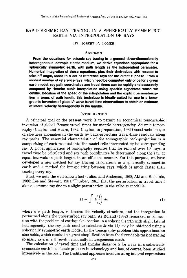
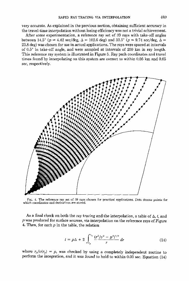
After some experimentation, a reference ray set of 39 rays with take-off angles between 14.5 ° (p = 4.42 sec/deg, A = 102.6 deg) and 33.5 ° (p = 9.74 sec/deg, A = 23.8 deg) was chosen for use in actual applications. The rays were spaced at intervals of 0.5 ° in take-off angle, and were sampled at intervals of 200 km in ray length. This reference ray system is illustrated in Figure 5. Ray path coordinates and travel times found by interpolating on this system are correct to within 0.05 km and 0.05 sec, respectively.

Fro. 4. The reference ray set of 39 rays chosen for practical applications. Dots denote points for which coordinates and derivatives are stored.

As a final check on both the ray tracing and the interpolation, a table of A, t, and p was produced for surface sources, via interpolation on the reference rays of Figure 4. Then, for each p in the table, the relation

frr r. ( r 2 / v 2 _ p2)1/2 t = p A + 2 d r

F (14)

where r p / v ( r p ) = p , was checked by using a completely independent routine to perform the integration, and it was found to hold to within 0.03 sec. Equation (14)

is derived by Bullen (1963), but it also follows simply by integrating

Ot Ot dt = -~ d A + , dr

Or

O O 0 O

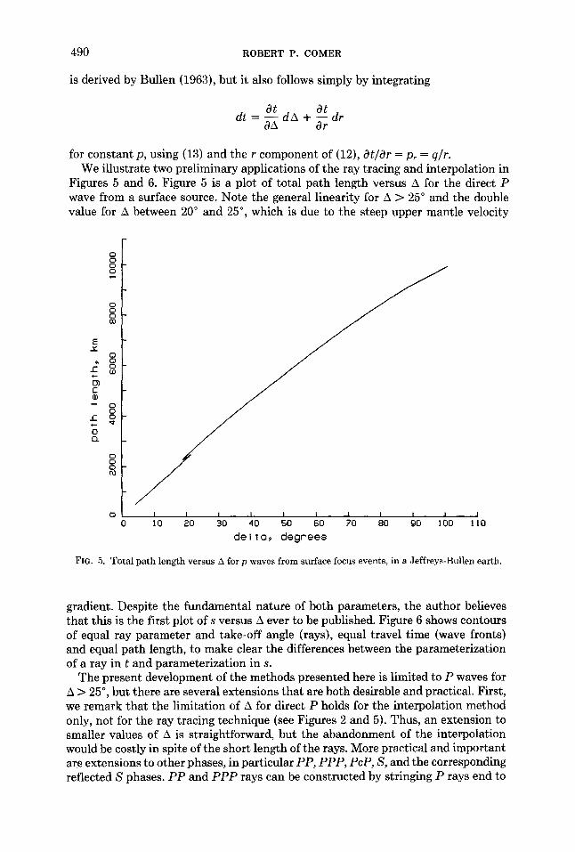
for constant p, using (13) and the r component of (12), Or/Or = Pr = q/r. We illustrate two preliminary applications of the ray tracing and interpolation in

Figures 5 and 6. Figure 5 is a plot of total path length versus A for the direct P wave from a surface source. Note the general linearity for A > 25 ° and the double value for A between 20 ° and 25 °, which is due to the steep upper mantle velocity

E

O

O) C

- - O O

cl

I I I I ! , i I I I I I

0 I0 20 30 40 SO 60 70 80 go I00 1 I0

dell09 degrees

490 ROBERT P. COMER

FIG. 5. Total path length versus A for p waves from surface focus events, in a Jeffreys-Bullen earth.

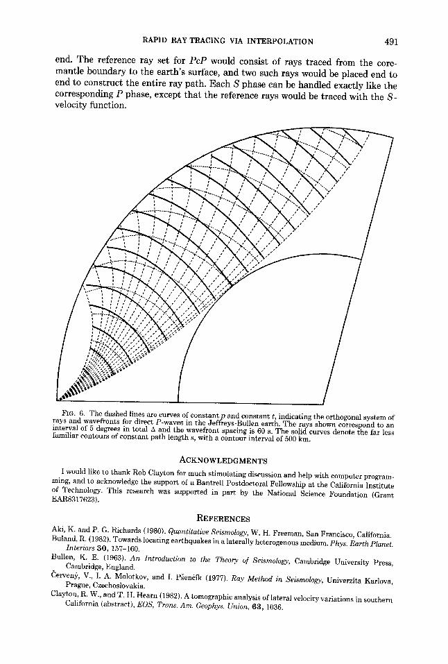
gradient. Despite the fundamental nature of both parameters, the author believes that this is the first plot of s versus A ever to be published. Figure 6 shows contours of equal ray parameter and take-off angle (rays), equal travel time (wave fronts) and equal path length, to make clear the differences between the parameterizafion of a ray in t and parameterization in s.

The present development of the methods presented here is limited to P waves for A > 25°, but there are several extensions that are both desirable and practical. First, we remark that the limitation of A for direct P holds for the interpolation method only, not for the ray tracing technique (see Figures 2 and 5). Thus, an extension to smaller values of A is straightforward, but the abandonment of the interpolation would be costly in spite of the short length of the rays. More practical and important are extensions to other phases, in particular PP, PPP, PcP, S, and the corresponding reflected S phases. PP and PPP rays can be constructed by stringing P rays end to

RAPID RAY TRACING VIA INTERPOLATION 491

end. The reference ray set for PcP would consist of rays traced from the core- mantle boundary to the earth's surface, and two such rays would be placed end to end to construct the entire ray path. Each S phase can be handled exactly like the corresponding P phase, except that the reference rays would be traced with the S- velocity function.

s~ J

, . J~ j J

, : • /

FIG. 6. The dashed lines are curves of constant p and constant t, indicating the orthogonal system of rays and wavefronts for direct P-waves in the Jeffreys-Bullen earth. The rays shown correspond to an interval of 5 degrees in total A and the wavefront spacing is 60 s. The solid curves denote the far less familiar contours of constant path length s, with a contour interval of 500 kin.

ACKNOWLEDGMENTS

I would like to thank Rob Clayton for much stimulating discussion and help with computer program- ming, and to acknowledge the support of a Bantrell Postdoctoral Fellowship at the California Institute of Technology. This research was supported in part by the National Science Foundation (Grant EAR8317623).

REFERENCES

Aki, K. and P. G. Richards (1980). Quantitative Seismology, W. H. Freeman, San Francisco, California. Buland, R. (1982). Towards locating earthquakes in a laterally heterogenous medium. Phys. Earth Planet.

Interiors 30, 157-160.

Bullen, K. E. (1963). An Introduction to the Theory of Seismology, Cambridge University Press, Cambridge, England.

Cerven~, V., I. A. Molotkov, and I. P~en~ik (1977). Ray Method in Seismology, Univerzita Karlova, Prague, Czechoslovakia.

Clayton, R. W., and T. H. Hearn {1982). A tomographic analysis of lateral velocity variations in southern California (abstract), EOS, Trans. Am. Geophys. Union, 63, 1036.

492 ROBERT P. COMER

Comer, R. P. and K. Aki (1981). Effects of lateral heterogeneity near an earthquake source on teleseismic ray paths (abstract), Earthquake Notes 52, 56.

Dahlquist, G. and A. Bjorck {1974). Numerical Methods, translated by N. Andersen, Prentice-Hall, Englewood Cliffs, New Jersey.

Forsythe, G. E., M. A. Malcolm, and C. B. Moler (1977). Computer Methods for Mathematical Compu- tations, Prentice-Hall, Englewood Cliffs, New Jersey.

Jacob, K. H. (1970). Three-dimensional seismic ray tracing in a laterally heterogeneous spherical earth. J. Geophys. Res. 75, 6675-6689.

Julian, B. R. (1970). Ray tracing in arbitrarily heterogenous media, Tech. Note 1970-45, Lincoln Lab., Massachusetts Institute of Technology, Cambridge, Massachusetts.

Julian, B. R. and D. L. Anderson (1968). Travel times, apparent velocities and amplitudes of body waves, Bull. Seism. Soc. Am. 58, 339-366.

Julian, B. R. and D. Gubbins (1977). Three-dimensional seismic ray tracing, J. Geophys. 43, 95-113. Lee, W. H. K. and S. W. Stewart (1981). Principles and Applications of Microearthquake Networks,

Advances in Geophysics, Suppl. 2, Academic Press, New York. Pereyra, V., W. H. K. Lee, and H. B. Keller (1980). Solving two-point seismic ray-tracing problems in a

heterogeneous medium, Part 1. A general adaptive finite difference method, Bull. Seism. Soc. Am. 70, 79-99.

Shampine, L. F. and M. K. Gordon (1975). Computer Solution of Ordinary Differential Equations: The Initial Value Problem. W. H. Freeman, San Francisco, California.

Thurber, C. H. (1981). Earth structure and earthquake locations in the Coyote Lake area, central California, Ph.D. Thesis, Massachusetts Institute of Technology, Cambridge, Massachusetts.

Yang, J. P. and W. H. K. Lee (1976). Preliminary investigations on computational methods for solving the two-point seismic ray-tracing problems in a heterogeneous and isotropic medium, U.S. Geol. Surv., Open-File Rept. 76-707, 1-66.

SEISMOLOGICAL LABORATORY CALIFORNIA INSTITUTE OF TECHNOLOGY PASADENA, CALIFORNIA 91125 CONTRIBUTION NO. 3942

Manuscript received 20 July 1983

APPENDIX

T h e ana ly t ic so lu t ion to (7) for the case of c o n s t a n t v a nd the a rb i t r a ry init ial

cond i t ions

r(O) = ro ri(O) = rio

A ( O ) = A 0 ~ i ( O ) = Aio

q(O) = qo qi(O) = qio

is

r(s)

A(s)

q(s)

ri(s)

Ai(s)

qi(8)

t ( o ) = ~

= (r$ + 2vqos + s2) ~/2

= Ao + t an -~ (q(s)/p) - t a n -~ (qo/P)

= qo + s /v

= (vqios + rorio)/r(s)

s[(s + 2vqo)(qorio - roqlo) - vroppi] = Aio + pro[r(s)]2

= qio

t ( s ) = to + s / v .