Bulletin of the JSME Vol.X, No.X, XXXXBulletin of the JSME Vol.X, No.X, XXXX PFC design method for SAC based on the stability theorem of the descriptor system and frequency response

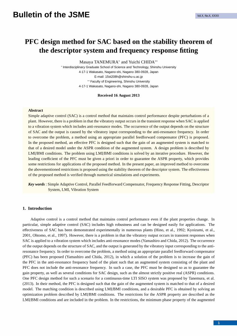
Bulletin of the JSME Vol.X, No.X, XXXX

PFC design method for SAC based on the stability theorem ofthe descriptor system and frequency response fitting

Masaya TANEMURA∗ and Yuichi CHIDA∗∗∗ Interdisciplinary Graduate School of Science and Technology, Shinshu University

4-17-1 Wakasato, Nagano-shi, Nagano 380-0928, Japan

E-mail: [email protected]∗∗ Faculty of Engineering, Shinshu University

4-17-1 Wakasato, Nagano-shi, Nagano 380-0928, Japan

Received 16 August 2013

AbstractSimple adaptive control (SAC) is a control method that maintains control performance despite perturbations of aplant. However, there is a problem in that the vibratory output occurs in the transient response when SAC is appliedto a vibration system which includes anti-resonance modes. The occurrence of the output depends on the structureof SAC and the output is caused by the vibratory input corresponding to the anti-resonance frequency. In orderto overcome the problem, a method using an appropriate parallel feedforward compensator (PFC) is proposed.In the proposed method, an effective PFC is designed such that the gain of an augmented system is matched tothat of a desired model under the ASPR condition of the augmented system. A design problem is described byLMI /BMI conditions. The problem using LMI/BMI conditions is solved by an iterative procedure. However, theleading coefficient of the PFC must be given a priori in order to guarantee the ASPR property, which providessome restrictions for applications of the proposed method. In the present paper, an improved method to overcomethe abovementioned restrictions is proposed using the stability theorem of the descriptor system. The effectivenessof the proposed method is verified through numerical simulations and experiments.

Key words: Simple Adaptive Control, Parallel Feedforward Compensator, Frequency Response Fitting, DescriptorSystem, LMI, Vibration System

1. Introduction

Adaptive control is a control method that maintains control performance even if the plant properties change. Inparticular, simple adaptive control (SAC) includes high robustness and can be designed easily for applications. Theeffectiveness of SAC has been demonstrated experimentally in numerous plants (Hino, et al., 1992; Kyoizumi, et al.,2001, Ohtomo, et al., 1997). However, there is a problem in that the vibratory output occurs in transient responses whenSAC is applied to a vibration system which includes anti-resonance modes (Yamashiro and Chida, 2012). The occurrenceof the output depends on the structure of SAC, and the output is generated by the vibratory input corresponding to the anti-resonance frequency. In order to overcome the problem, a method using an appropriate parallel feedforward compensator(PFC) has been proposed (Yamashiro and Chida, 2012), in which a solution of the problem is to increase the gain ofthe PFC in the anti-resonance frequency band of the plant such that an augmented system consisting of the plant andPFC does not include the anti-resonance frequency. In such a case, the PFC must be designed so as to guarantee thegain property, as well as several conditions for SAC design, such as the almost strictly positive real (ASPR) conditions.One PFC design method for such a scenario for a continuous-time LTI SISO system was proposed by Tanemura, et al.(2013). In their method, the PFC is designed such that the gain of the augmented system is matched to that of a desiredmodel. The matching condition is described using LMI/BMI conditions, and a desirable PFC is obtained by solving anoptimization problem described by LMI/BMI conditions. The restrictions for the ASPR property are described as theLMI /BMI conditions and are included in the problem. In the restrictions, the minimum phase property of the augmented

1


system is described by the Lyapunov inequality by Tanemura, et al. (2013). In such a case, the leading coefficient of thenumerator of the PFC is assumed to be given a priori. However, it is difficult to obtain the leading coefficient in advancein some cases. The present paper introduces descriptor systems in order to overcome the restrictions. The description ofa descriptor system possesses redundancy compared with the state space representation. Then, the stability theorem ofa descriptor system proposed by Uezato and Ikeda (1998) is used in order to guarantee the minimum phase property ofthe augmented system. The proposed method requires no a priori information on the coefficients of the PFC, which aredetermined automatically in the proposed method because of redundancy of a descriptor system. On the other hand, auseful design method has been proposed by Mizumoto, et al. (2010). The method employs the desired model minus theplant as the PFC. The method can easily design the PFC without optimized calculation. However, if the order of the plantor the desired model is high, the order of the PFC increases because it depends on the order of the plant and the desiredmodel. In contrast, the proposed method can design a low order PFC compared with the method proposed by Mizumoto,et al. (2010). The effectiveness of the proposed method is verified through not only simulations but also experimentsusing a mechanical vibration system. In addition, the robustness of the proposed design method is discussed in the presentpaper.

2. Problem statement2.1. Plant

The present paper investigates the following continuous-time LTI SISO plant:

Gp(s)

xp(t) = Apxp(t) + bpup(t)yp(t) = cpxp(t)

(1)

Ap ∈ Rnp×np, bp ∈ Rnp×1, cp ∈ R1×np

whereRn×m denotes ann-by-m real matrix set. The plant is assumed to be (Ap, bp)-controllable and (cp, Ap)-observable.The nominal parameters ofGp(s) are assumed to be known.

2.2. Design of the SACAn nm-th order SISO reference model, which is a design parameter, is described as follows:

Gm(s)

xm(t) = Amxm(t) + bmum(t)ym(t) = cmxm(t)

(2)

Am ∈ Rnm×nm, bm ∈ Rnm×1, cm ∈ R1×nm

whereAm is a stable matrix. The control objective is for the output of the plant to follow that of the reference model. Thefollowing are the assumptions regarding the plant and the reference model used to design the SAC.Assumptions (Mizumoto and Iwai, 2001)

1) The plant has ASPR characteristics.

2) The plant and the reference model have command generator tracker (CGT) solutions.

3) um(t) is differentiable.

The ASPR property is defined as follows.Definition (Mizumoto and Iwai, 2001)Gp(s) has ASPR property when a static output feedback that a closed-loop system with the static output feedback becomesstrictly positive real exists.Sufficient conditions of the ASPR property are described at the section of 3.2. A lot of plants hardly have the ASPRproperty of Assumption 1). A PFC is generally introduced in order to satisfy Assumption 1). The PFC is designed toensure that the augmented system

Ga(s) := Gp(s) +G f (s) (3)

has ASPR characteristics. Where,G f (s) is the transfer function of the PFC. SinceGa(s) is ASPR, SAC can be applied toGa(s). The control objective is to satisfy the following equation under the above assumptions:

limt→∞

ea(t) = 0, ea(t) = ya(t) − ym(t) (4)

2


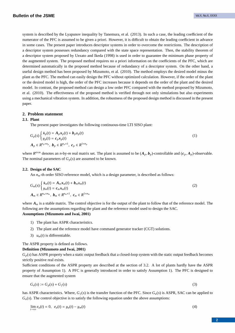
Fig. 1 This block diagram expresses the SAC system with the PFC.Gp(s), G f (s), andGm(s) are the plant, PFC,and the reference model, respectively.ku(t) and kx(t) are adaptive feedforward gains, andke(t) is anadaptive feedback gain.

Where,ya(t) is the output ofGa(s).A block diagram of the SAC system is shown in Fig. 1. The SAC is described by the following equations:

up(t) = k(t)T z(t) (5)

z(t) =[ea(t) xm(t)T um(t)

]Tk(t) =

[ke(t) kx(t)T ku(t)

]Tk(t) = kP(t) + kI (t) (6)

kP(t) = −ΓPz(t)ea(t) (7)

kI (t) = −ΓI z(t)ea(t) − σ(t)kI (t) (8)

σ(t) =e2

a(t)

1+ e2a(t)σ1 + σ2 (9)

ΓP = ΓTP > 0, ΓI = Γ

TI > 0, σ1 > 0, σ2 ≥ 0

whereku(t) and kx(t) are adaptive feedforward gains, andke(t) is an adaptive feedback gain. The PI-type adaptive lawusing theσ-modification method is used as the adaptive adjusting law. Here,ΓP andΓI are adaptive adjusting gainmatrixes.kI (t) stabilizes the SAC control system.kP(t) plays a role in suppressing vibration of convergence of adaptivegains. The initial value ofkI (t) is a design parameter.

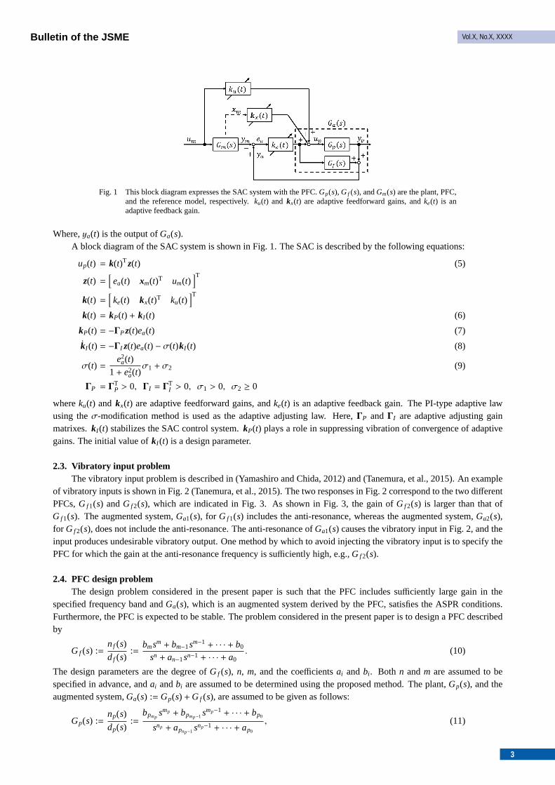
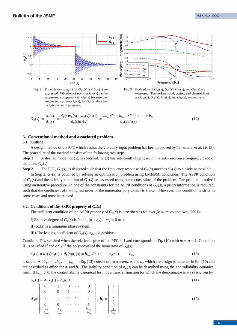
2.3. Vibratory input problemThe vibratory input problem is described in (Yamashiro and Chida, 2012) and (Tanemura, et al., 2015). An example

of vibratory inputs is shown in Fig. 2 (Tanemura, et al., 2015). The two responses in Fig. 2 correspond to the two differentPFCs,G f 1(s) andG f 2(s), which are indicated in Fig. 3. As shown in Fig. 3, the gain ofG f 2(s) is larger than that ofG f 1(s). The augmented system,Ga1(s), for G f 1(s) includes the anti-resonance, whereas the augmented system,Ga2(s),for G f 2(s), does not include the anti-resonance. The anti-resonance ofGa1(s) causes the vibratory input in Fig. 2, and theinput produces undesirable vibratory output. One method by which to avoid injecting the vibratory input is to specify thePFC for which the gain at the anti-resonance frequency is sufficiently high, e.g.,G f 2(s).

2.4. PFC design problemThe design problem considered in the present paper is such that the PFC includes sufficiently large gain in the

specified frequency band andGa(s), which is an augmented system derived by the PFC, satisfies the ASPR conditions.Furthermore, the PFC is expected to be stable. The problem considered in the present paper is to design a PFC describedby

G f (s) :=nf (s)

df (s):=

bmsm + bm−1sm−1 + · · · + b0

sn + an−1sn−1 + · · · + a0. (10)

The design parameters are the degree ofG f (s), n, m, and the coefficientsai andbi . Both n andm are assumed to bespecified in advance, andai andbi are assumed to be determined using the proposed method. The plant,Gp(s), and theaugmented system,Ga(s) := Gp(s) +G f (s), are assumed to be given as follows:

Gp(s) :=np(s)

dp(s):=

bpmpsmp + bpmp−1 smp−1 + · · · + bp0

snp + apnp−1 snp−1 + · · · + ap0

, (11)

3


Fig. 2 Time history ofup(t) for G f 1(s) andG f 2(s) areexpressed. Vibration ofup(t) for G f 2(s) can besuppressed compared withG f 1(s) because theaugmented system,Ga2(s), for G f 2(s) does notinclude the anti-resonance.

Fig. 3 Bode plots ofGa1(s), Ga2(s), G f 1(s), andG f 2(s) areexpressed. The broken, solid, dotted, and chained linesareGa1(s), Ga2(s), G f 1(s), andG f 2(s), respectively.

Ga(s) :=na(s)da(s)

:=df (s)np(s) + dp(s)nf (s)

dp(s)df (s)=

bamasma + bama−1 sma−1 + · · · + ba0

dp(s)df (s). (12)

3. Conventional method and associated problem3.1. Outline

A design method of the PFC which avoids the vibratory input problem has been proposed by Tanemura, et al. (2013).The procedure of the method consists of the following two steps.Step 1 A desired model,Gr (s), is specified.Gr (s) has sufficiently high gain in the anti-resonance frequency band ofthe plant,Gp(s).Step 2 The PFC,G f (s), is designed such that the frequency response ofGa(s) matchesGr (s) as closely as possible.

In Step 2,G f (s) is obtained by solving an optimization problem using LMI/BMI conditions. The ASPR conditionof Ga(s) and the stability condition ofG f (s) are assessed using some constraints of the problem. The problem is solvedusing an iterative procedure. In one of the constraints for the ASPR conditions ofGa(s), a priori information is required,such that the coefficient of the highest order of the numerator polynomial is known. However, this condition is strict insome cases and must be relaxed.

3.2. Conditions of the ASPR property ofGa(s)The sufficient condition of the ASPR property ofGa(s) is described as follows (Mizumoto and Iwai, 2001):

I) Relative degree ofGa(s) is 0 or 1, (n+ np) −ma = 0 or 1.

II) Ga(s) is a minimum phase system.

III) The leading coefficient ofGa(s), bama, is positive.

Condition I) is satisfied when the relative degree of the PFC is 1 and corresponds to Eq. (10) withm = n− 1. ConditionII) is satisfied if and only if the polynomial of the numerator ofGa(s),

na(s) = df (s)np(s) + dp(s)nf (s) = bamasma + · · · + bai s

i + · · · + ba0 (13)

is stable. Allba0, · · · ,bai , · · · ,bamain Eq. (13) consist of parameters,ai andbi , which are design parameters in Eq. (10) and

are described as affine forai andbi . The stability condition ofna(s) can be described using the controllability canonicalform. If bama

, 0, the controllability canonical form of a transfer function for which the denominator isna(s) is given by

xa (t) = Aaxa(t) + baua(t), (14)

Aa=

0 1 0 · · · 00 0 1 · · · 0...

.... . .

. . ....

0 0 · · · · · · 1

− ba0bama

− ba1bama

· · · · · · − bama−1

bama

, ba =

00...

01

bama

. (15)

4


The system of Eq. (14) is stable if and only if there exists a matrixPa which satisfies

PaAa + ATa Pa < 0, Pa > 0. (16)

By finding Pa and Aa in Eq. (16) at the same time, condition II) is guaranteed. In this case, Eq. (16) is not an LMIcondition but rather a BMI condition forAa andPa. If Aa is a known constant matrix, Eq. (16) can be solved as LMI forPa. On the other hand, ifPa is a known constant matrix, Eq. (16) can be solved as a LMI forAa. Thus, the above twoprocedures are executed iteratively to solve the BMI problem as LMIs. However, there is another difficulty in solving theproblem such that Eq. (15) is not affine for a design parameter of 1/bama

in Aa. In order to modifyAa to be affine, it isassumed thatbama

is given a priori and a specified fixed constant is used forbama. Here,bama

consists ofbn−1, as follows:

bama=

bpmp+ bn−1 (γp = 1)

bn−1 (γp ≥ 2) ,(17)

whereγp := np − mp is the relative degree ofGp(s). bpmpis a parameter ofGp(s) and is given. However,bn−1 is

a design parameter and so must be given a priori. Then, parametersbai , with the exception ofbama, are affine for

a0, . . . ,an−1,b0, . . . , bn−2. Note that, in the conventional method,bamamust be specified in advance. However, since a

suitable value of the leading coefficient,bn−1, cannot be given in realistic situations,bamamust be determined in an appro-

priate manner. Therefore, a modified method by which to overcome this requirement is proposed in the following section.Moreover,bama

is specified to be positive in order to satisfy condition III).

3.3. Condition for frequency matching ofGa(s) to Gr(s)The desired model, described asGr (s), which does not include the anti-resonance, is specified for fitting the frequency

responses ofGa(s) andGr (s). By describing the matching condition using LMI, the PFC design problem becomes a convexoptimization problem. In this case,Gr (s) must be designed such that the anti-resonance is not included and the ASPRproperty is maintained. An error transfer function (Chida and Nishimura, 2008) is described as follows:

E(ω) := M(ω)Gr ( jω) − M(ω)(Gp( jω) +G f ( jω)

)(18)

whereM(ω) is a frequency-dependent weighting function, andGp(s) andG f (s) are defined in Eq. (11) and (10). Equation(18) shows the matching error betweenGa( jω) andGr ( jω), respectively. Equation (18) is, however, not affine with respectto parametersai , bi . Thus,M(ω) is specified such thatM(ω) = df ( jω)/d( jω). Here,d( jω) is a known polynomial of then-th degree. SubstitutingM(ω) = df ( jω)/d( jω) into Eq. (18) yields

E(ω) =(Gr ( jω) −Gp( jω)

) df ( jω)

d( jω)−

nf ( jω)

d( jω)

=Gr ( jω) −Gp( jω)

d( jω)

[1 jω · · · ( jω)n−1 ( jω)n

]

a0

a1...

an−1

1

− 1

d( jω)

[1 jω · · · ( jω)n−2 ( jω)n−1

]

b0

b1...

bn−2

bn−1

= [Φr

0(ω) +Φra(ω)a+Φr

b(ω)b] + j[Φi0(ω) +Φi

a(ω)a+Φib(ω)b]

= Er (ω) + jE i(ω), (19)

a := [a0, . . . ,an−1]T, b := [b0, . . . , bn−2]T

whereΦr0 andΦi

0 are independent terms ofa and b, Φra andΦi

a are terms of the coefficients ofa, andΦrb andΦi

b areterms of the coefficients ofb. Assuming thatxT := [aT, bT], which is a design vector, the affine equation forx is derivedas follows:Er (ω)

Ei(ω)

= Φr0(ω)Φi

0(ω)

+ Φra(ω) Φr

b(ω)Φi

a(ω) Φib(ω)

x= β(ω) + α(ω)x. (20)

Equation (20) is intractable because Eq. (20) is a continuous function forω. Therefore, errors in the discrete frequencydataωk, which are sampled at N-points, are considered. Taking the discrete frequency dataωk simplifies the problem.

5


The following error objective functionJ:

J(x) :=N∑

k=1

[Er (ωk) Ei(ωk)

] Er (ωk)Ei(ωk)

= xTHTHx + 2gTHx + gTg (21)

is introduced usingωk, where

H :=

α(ω1)...

α(ωN)

, g :=

β(ω1)...

β(ωN)

. (22)

WhenH has full rank,HTH is a non-singular matrix. Thus,J < γ is represented by the LMI condition: γ − 2gTHx − gTg xTHT

Hx I

> 0 (23)

by settingγ and using the Schur complement. The minimization problem ofJ is equivalent to aγ-minimization problem.The LMI condition of Eq. (23) is easy to solve as a convex problem.

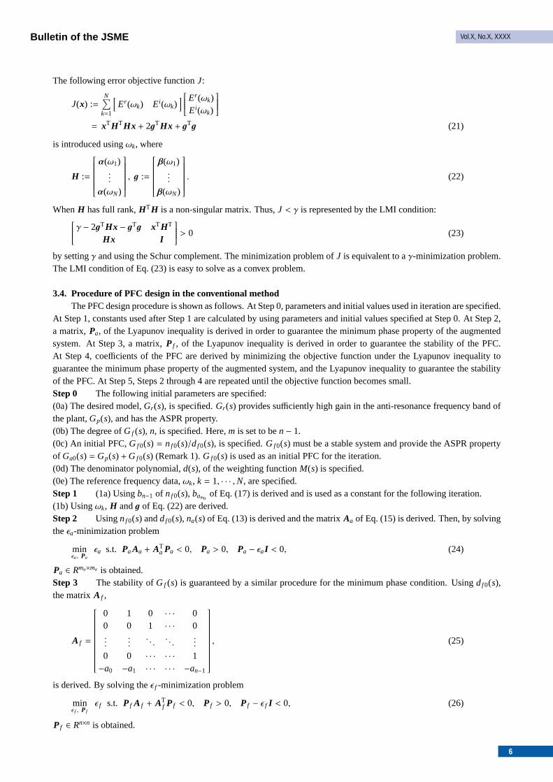
3.4. Procedure of PFC design in the conventional methodThe PFC design procedure is shown as follows. At Step 0, parameters and initial values used in iteration are specified.

At Step 1, constants used after Step 1 are calculated by using parameters and initial values specified at Step 0. At Step 2,a matrix,Pa, of the Lyapunov inequality is derived in order to guarantee the minimum phase property of the augmentedsystem. At Step 3, a matrix,Pf , of the Lyapunov inequality is derived in order to guarantee the stability of the PFC.At Step 4, coefficients of the PFC are derived by minimizing the objective function under the Lyapunov inequality toguarantee the minimum phase property of the augmented system, and the Lyapunov inequality to guarantee the stabilityof the PFC. At Step 5, Steps 2 through 4 are repeated until the objective function becomes small.Step 0 The following initial parameters are specified:(0a) The desired model,Gr (s), is specified.Gr (s) provides sufficiently high gain in the anti-resonance frequency band ofthe plant,Gp(s), and has the ASPR property.(0b) The degree ofG f (s), n, is specified. Here,m is set to ben− 1.(0c) An initial PFC,G f 0(s) = nf 0(s)/df 0(s), is specified.G f 0(s) must be a stable system and provide the ASPR propertyof Ga0(s) = Gp(s) +G f 0(s) (Remark 1).G f 0(s) is used as an initial PFC for the iteration.(0d) The denominator polynomial,d(s), of the weighting functionM(s) is specified.(0e) The reference frequency data,ωk, k = 1, · · · ,N, are specified.Step 1 (1a) Usingbn−1 of nf 0(s), bama

of Eq. (17) is derived and is used as a constant for the following iteration.(1b) Usingωk, H andg of Eq. (22) are derived.Step 2 Usingnf 0(s) anddf 0(s), na(s) of Eq. (13) is derived and the matrixAa of Eq. (15) is derived. Then, by solvingtheϵa-minimization problem

minϵa, Pa

ϵa s.t. PaAa + ATa Pa < 0, Pa > 0, Pa − ϵaI < 0, (24)

Pa ∈ Rma×ma is obtained.Step 3 The stability ofG f (s) is guaranteed by a similar procedure for the minimum phase condition. Usingdf 0(s),the matrixA f ,

A f =

0 1 0 · · · 00 0 1 · · · 0...

.... . .

. . ....

0 0 · · · · · · 1−a0 −a1 · · · · · · −an−1

, (25)

is derived. By solving theϵ f -minimization problem

minϵ f , Pf

ϵ f s.t. Pf A f + ATf Pf < 0, Pf > 0, Pf − ϵ f I < 0, (26)

Pf ∈ Rn×n is obtained.

6


Step 4 Using Pa andPf obtained in Steps 2 and 3, theγ-minimization problem

minγ, x, Aa, A f

γ s.t.

γ − 2gTHx − gTg xTHT

Hx I

> 0 (27)

PaAa + ATa Pa < 0 (28)

Pf A f + ATf Pf < 0 (29)

is solved forAa and A f , whereAa and A f are variables consisting ofx and their structures are Eq. (15) and Eq. (25),respectively. Here,G f (s), which consists of the obtained solution,x, is a stable system and gives the ASPR property ofGa(s).Step 5 Steps 2 through 4 are repeated untilγ becomes sufficiently small. Here,G f (s) = nf (s)/df (s) used in Steps 2and 3 is an updated solution obtained in Step 4.Remark 1: Increasing the gain of the PFC simplifies the design of the PFC which provides the ASPR property ofGa(s).Remark 2: At Step 4,Aa andA f which minimizeγ for Pa andPf are obtained. When the procedure is executed iterativelyby Step 5, and Eq. (24) and Eq. (26) using theseAa andA f are solved in Steps 2 and 3,γ of Eq. (27) is invariant. Thus,γdoes not deteriorate in Steps 2 and 3. Therefore,γ is guaranteed to decrease monotonically by this procedure.At (1a) of Step 1, the leading coefficient,bn−1, of the PFC is specified and is treated as a constant at the optimal problem.However, ifbn−1 cannot be specified appropriately, the result of the frequency response fitting deteriorates. In order totreatbn−1 as a design parameter of the optimal problem, a method using a descriptor system is proposed in the followingchapter.

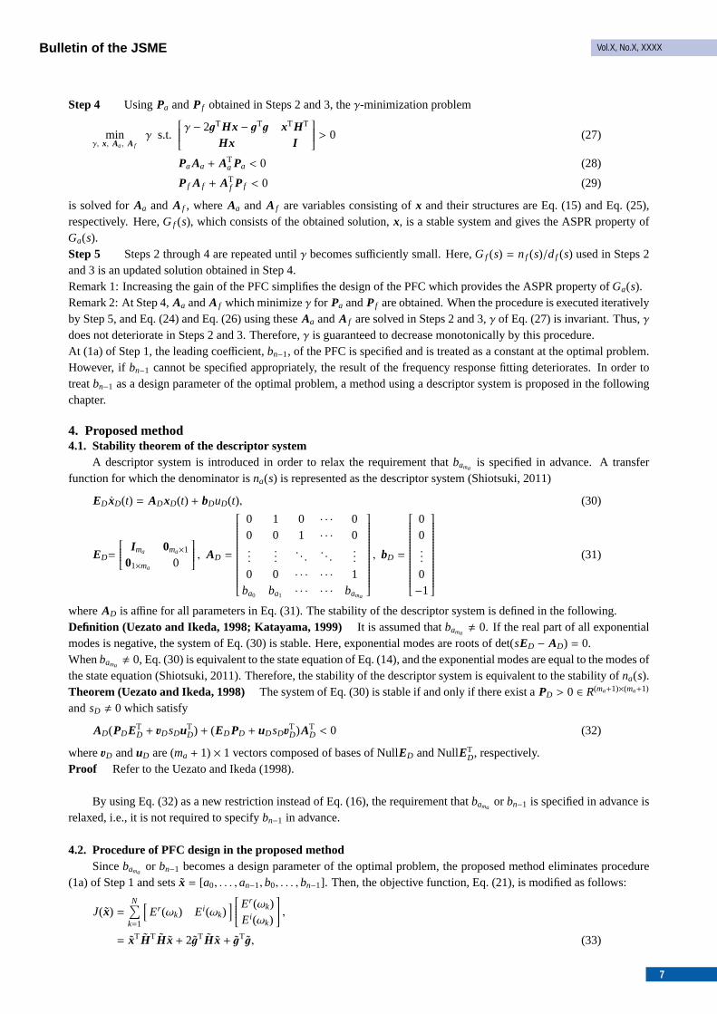
4. Proposed method4.1. Stability theorem of the descriptor system

A descriptor system is introduced in order to relax the requirement thatbamais specified in advance. A transfer

function for which the denominator isna(s) is represented as the descriptor system (Shiotsuki, 2011)

ED xD(t) = ADxD(t) + bDuD(t), (30)

ED=

Ima 0ma×1

01×ma 0

, AD =

0 1 0 · · · 00 0 1 · · · 0...

.... . .

. . ....

0 0 · · · · · · 1ba0 ba1 · · · · · · bama

, bD =

00...

0−1

(31)

whereAD is affine for all parameters in Eq. (31). The stability of the descriptor system is defined in the following.Definition (Uezato and Ikeda, 1998; Katayama, 1999) It is assumed thatbama

, 0. If the real part of all exponentialmodes is negative, the system of Eq. (30) is stable. Here, exponential modes are roots of det(sED − AD) = 0.Whenbama

, 0, Eq. (30) is equivalent to the state equation of Eq. (14), and the exponential modes are equal to the modes ofthe state equation (Shiotsuki, 2011). Therefore, the stability of the descriptor system is equivalent to the stability ofna(s).Theorem (Uezato and Ikeda, 1998) The system of Eq. (30) is stable if and only if there exist aPD > 0 ∈ R(ma+1)×(ma+1)

andsD , 0 which satisfy

AD(PDETD + uDsDuT

D) + (ED PD + uDsDuTD)AT

D < 0 (32)

whereuD anduD are (ma + 1)× 1 vectors composed of bases of NullED and NullETD, respectively.

Proof Refer to the Uezato and Ikeda (1998).

By using Eq. (32) as a new restriction instead of Eq. (16), the requirement thatbamaor bn−1 is specified in advance is

relaxed, i.e., it is not required to specifybn−1 in advance.

4.2. Procedure of PFC design in the proposed methodSincebama

or bn−1 becomes a design parameter of the optimal problem, the proposed method eliminates procedure(1a) of Step 1 and setsx = [a0, . . . ,an−1,b0, . . . ,bn−1]. Then, the objective function, Eq. (21), is modified as follows:

J(x) =N∑

k=1

[Er (ωk) Ei(ωk)

] Er (ωk)Ei(ωk)

,= xTHTH x + 2gTH x + gTg, (33)

7


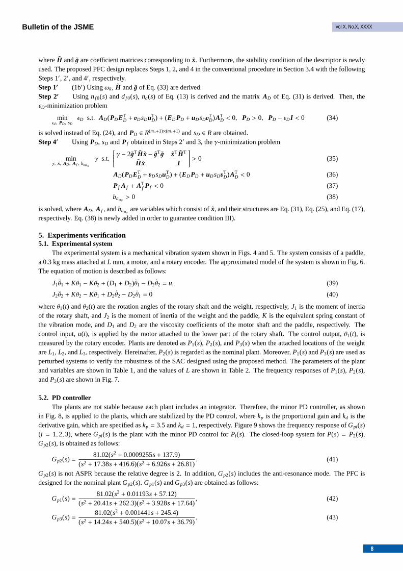
whereH andg are coefficient matrices corresponding tox. Furthermore, the stability condition of the descriptor is newlyused. The proposed PFC design replaces Steps 1, 2, and 4 in the conventional procedure in Section 3.4 with the followingSteps 1′, 2′, and 4′, respectively.Step1′ (1b′) Usingωk, H andg of Eq. (33) are derived.Step 2′ Using nf 0(s) anddf 0(s), na(s) of Eq. (13) is derived and the matrixAD of Eq. (31) is derived. Then, theϵD-minimization problem

minϵd, PD, sD

ϵD s.t. AD(PDETD + uDsDuT


D < 0, PD > 0, PD − ϵD I < 0 (34)

is solved instead of Eq. (24), andPD ∈ R(ma+1)×(ma+1) andsD ∈ R are obtained.Step4′ Using PD, sD andPf obtained in Steps 2′ and 3, theγ-minimization problem

minγ, x, AD, A f , bama

γ s.t.

γ − 2gTH x − gTg xTHT

H x I

> 0 (35)

AD(PDETD + uDsDuT


D < 0 (36)

Pf A f + ATf Pf < 0 (37)

bama> 0 (38)

is solved, whereAD, A f , andbamaare variables which consist ofx, and their structures are Eq. (31), Eq. (25), and Eq. (17),

respectively. Eq. (38) is newly added in order to guarantee condition III).

5. Experiments verification5.1. Experimental system

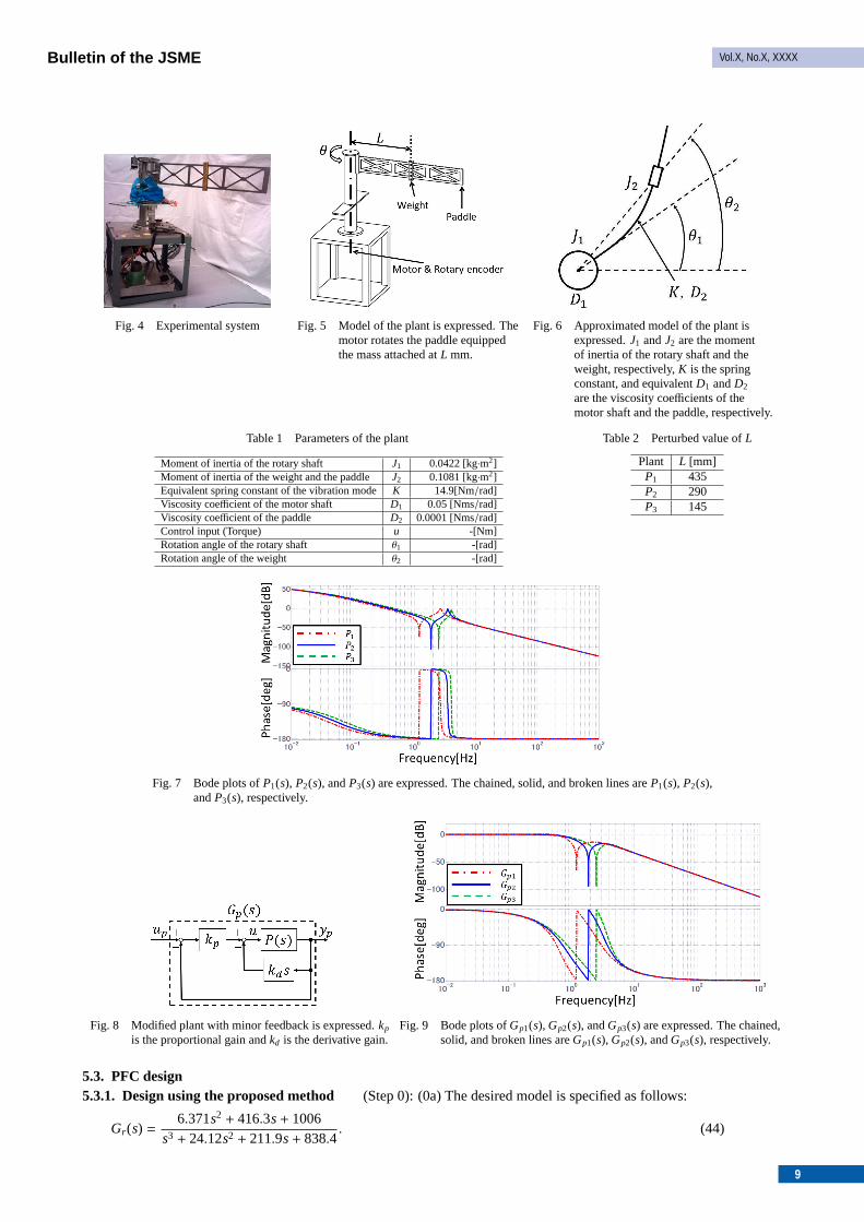
The experimental system is a mechanical vibration system shown in Figs. 4 and 5. The system consists of a paddle,a 0.3 kg mass attached atL mm, a motor, and a rotary encoder. The approximated model of the system is shown in Fig. 6.The equation of motion is described as follows:

J1θ1 + Kθ1 − Kθ2 + (D1 + D2)θ1 − D2θ2 = u, (39)

J2θ2 + Kθ2 − Kθ1 + D2θ2 − D2θ1 = 0 (40)

whereθ1(t) andθ2(t) are the rotation angles of the rotary shaft and the weight, respectively,J1 is the moment of inertiaof the rotary shaft, andJ2 is the moment of inertia of the weight and the paddle,K is the equivalent spring constant ofthe vibration mode, andD1 and D2 are the viscosity coefficients of the motor shaft and the paddle, respectively. Thecontrol input,u(t), is applied by the motor attached to the lower part of the rotary shaft. The control output,θ1(t), ismeasured by the rotary encoder. Plants are denoted asP1(s), P2(s), andP3(s) when the attached locations of the weightareL1, L2, andL3, respectively. Hereinafter,P2(s) is regarded as the nominal plant. Moreover,P1(s) andP3(s) are used asperturbed systems to verify the robustness of the SAC designed using the proposed method. The parameters of the plantand variables are shown in Table 1, and the values ofL are shown in Table 2. The frequency responses ofP1(s), P2(s),andP3(s) are shown in Fig. 7.

5.2. PD controllerThe plants are not stable because each plant includes an integrator. Therefore, the minor PD controller, as shown

in Fig. 8, is applied to the plants, which are stabilized by the PD control, wherekp is the proportional gain andkd is thederivative gain, which are specified askp = 3.5 andkd = 1, respectively. Figure 9 shows the frequency response ofGpi(s)(i = 1,2,3), whereGpi(s) is the plant with the minor PD control forPi(s). The closed-loop system forP(s) = P2(s),Gp2(s), is obtained as follows:

Gp2(s) =81.02(s2 + 0.0009255s+ 137.9)

(s2 + 17.38s+ 416.6)(s2 + 6.926s+ 26.81). (41)

Gp2(s) is not ASPR because the relative degree is 2. In addition,Gp2(s) includes the anti-resonance mode. The PFC isdesigned for the nominal plantGp2(s). Gp1(s) andGp3(s) are obtained as follows:

Gp1(s) =81.02(s2 + 0.01193s+ 57.12)

(s2 + 20.41s+ 262.3)(s2 + 3.928s+ 17.64), (42)

Gp3(s) =81.02(s2 + 0.001441s+ 245.4)

(s2 + 14.24s+ 540.5)(s2 + 10.07s+ 36.79). (43)

8


Fig. 4 Experimental system Fig. 5 Model of the plant is expressed. Themotor rotates the paddle equippedthe mass attached atL mm.

Fig. 6 Approximated model of the plant isexpressed.J1 andJ2 are the momentof inertia of the rotary shaft and theweight, respectively,K is the springconstant, and equivalentD1 andD2

are the viscosity coefficients of themotor shaft and the paddle, respectively.

Table 1 Parameters of the plant

Moment of inertia of the rotary shaft J1 0.0422 [kg·m2]Moment of inertia of the weight and the paddle J2 0.1081 [kg·m2]Equivalent spring constant of the vibration modeK 14.9[Nm/rad]Viscosity coefficient of the motor shaft D1 0.05 [Nms/rad]Viscosity coefficient of the paddle D2 0.0001 [Nms/rad]Control input (Torque) u -[Nm]Rotation angle of the rotary shaft θ1 -[rad]Rotation angle of the weight θ2 -[rad]

Table 2 Perturbed value ofL

Plant L [mm]P1 435P2 290P3 145

Fig. 7 Bode plots ofP1(s), P2(s), andP3(s) are expressed. The chained, solid, and broken lines areP1(s), P2(s),andP3(s), respectively.

Fig. 8 Modified plant with minor feedback is expressed.kp

is the proportional gain andkd is the derivative gain.Fig. 9 Bode plots ofGp1(s), Gp2(s), andGp3(s) are expressed. The chained,

solid, and broken lines areGp1(s), Gp2(s), andGp3(s), respectively.

5.3. PFC design5.3.1. Design using the proposed method (Step 0): (0a) The desired model is specified as follows:

Gr (s) =6.371s2 + 416.3s+ 1006

s3 + 24.12s2 + 211.9s+ 838.4. (44)

9


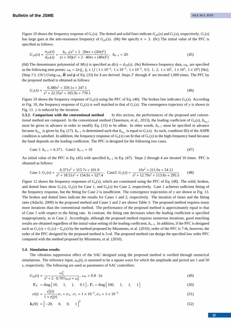
Figure 10 shows the frequency response ofGr (s). The dotted and solid lines indicateGp2(s) andGr (s), respectively.Gr (s)has large gain at the anti-resonance frequency ofGp2(s). (0b) We specifyn = 3. (0c) The initial value of the PFC isspecified as follows:

G f 0(s) =nf 0(s)

df 0(s)=

bn−1(s2 + 2 · 20πs+ (20π)2)(s+ 10)(s2 + 2 · 40πs+ (40π)2)

, bn−1 = 20. (45)

(0d) The denominator polynomial ofM(s) is specified asd(s) = df 0(s). (0e) Reference frequency data,ωk, are specifiedas the following nine points:ωk = 2π fk, fk ∈ { f | 1×10−4, 1×10−3, 1×10−2, 0.5, 1, 2, 1×102, 1×103, 1×104} [Hz].(Step 1′): (1b′) Usingωk, H andg of Eq. (33) forx are derived. Steps 2′ through 4′ are iterated 1,000 times. The PFC bythe proposed method is obtained as follows:

G f (s) =6.380s2 + 359.1s+ 247.1

s3 + 22.55s2 + 165.9s+ 770.1(46)

Figure 10 shows the frequency response ofGa(s) using the PFC of Eq. (46). The broken line indicatesGa(s). Accordingto Fig. 10, the frequency response ofGa(s) is well matched to that ofGr (s). The convergence trajectory ofγ is shown inFig. 11.γ is reduced by the iteration.5.3.2. Comparison with the conventional method In this section, the performances of the proposed and conven-tional method are compared. In the conventional method (Tanemura, et al., 2013), the leading coefficient ofGa(s), bama

,must be given in advance in order to modify Eq. (15) to be affine. In other words,bn−1 must be specified in advancebecausebama

is given by Eq. (17).bn−1 is determined such thatbamais equal toGr (s). As such, condition III) of the ASPR

condition is satisfied. In addition, the frequency response ofGa(s) can fit that ofGr (s) in the high-frequency band becausethe band depends on the leading coefficient. The PFC is designed for the following two cases.

Case 1:bn−1 = 6.371, Case2:bn−1 = 10 (47)

An initial value of the PFC is Eq. (45) with specifiedbn−1 in Eq. (47). Steps 2 through 4 are iterated 10 times. PFC isobtained as follows:

Case 1:G f (s) =6.371s2 + 315.7s+ 101.9

s3 + 18.51s2 + 154.9s+ 527.4, Case2:G f (s) =

10s2 + 211.0s+ 54.11s3 + 12.79s2 + 113.8s+ 295.5

(48)

Figure 12 shows the frequency responses ofGa(s), which are constituted using the PFC of Eq. (48). The solid, broken,and dotted lines showGr (s), Ga(s) for Case 1, andGa(s) for Case 2, respectively. Case 1 achieves sufficient fitting ofthe frequency response, but the fitting for Case 2 is insufficient. The convergence trajectories ofγ are shown in Fig. 13.The broken and dotted lines indicate the results for Cases 1 and 2, respectively. The iteration of times and the fittingrates (Adachi, 2009) in the proposed method and Cases 1 and 2 are shown Table 3. The proposed method requires manymore iterations than the conventional method. The performance of the proposed method is approximately equal to thatof Case 1 with respect to the fitting rate. In contrast, the fitting rate decreases when the leading coefficient is specifiedinappropriately, as in Case 2. Accordingly, although the proposed method requires numerous iterations, good matchingresults are obtained regardless of the initial value setting of the leading coefficient,bn−1. In addition, if the PFC is designedsuch asG f (s) = Gr (s)−Gp(s) by the method proposed by Mizumoto, et al. (2010), order of the PFC is 7-th, however, theorder of the PFC designed by the proposed method is 3-rd. The proposed method can design the specified low order PFCcompared with the method proposed by Mizumoto, et al. (2010).

5.4. Simulation resultsThe vibration suppression effect of the SAC designed using the proposed method is verified through numerical

simulations. The reference input,um(t), is assumed to be a square wave for which the amplitude and period are 1 and 50s, respectively. The following are used as parameters of SAC controllers:

Gm(s) =ω2

n

s2 + 2 · 0.707ωns+ ω2n, ωn = 0.8 · 2π (49)

ΓP = diag{10, 1, 1, 0.1

}, ΓI = diag

{100, 1, 1, 1

}(50)

σ(t) =e2

a(t)

1+ e2a(t)σ1 + σ2, σ1 = 1× 10−2, σ2 = 1× 10−5 (51)

kI (0) =[−20, 0, 0, 1

]T(52)

10


Fig. 10 Bode plot ofGp2(s), Gr (s) andGa(s) for proposed methodare expressed. The chained, solid, and broken lines areGp2(s), Gr (s), andGa(s), respectively. The frequencyresponse ofGa(s) is well matched to that ofGr (s).

Fig. 11 Trajectory ofγ is expressed.γ is reduced by the iteration.

Fig. 12 Bode plots ofGr (s), Ga(s) for Case 1, andGa(s) for Case 2are expressed. The solid, broken, and chained lines areGr (s), Ga(s) for Case 1, andGa(s) for Case 2, respectively.Case 1 achieves sufficient fitting of the frequency response,but the fitting for Case 2 is insufficient.

Fig. 13 Trajectories ofγ for Cases 1 and 2 are expressed.γ are reduced by the iteration.

Table 3 Performance of the Proposed Method and Cases 1 and 2

Proposed method Case1 Case2Iteration of times 1000 10 10Fitting rate[%] 96.0 98.6 86.8

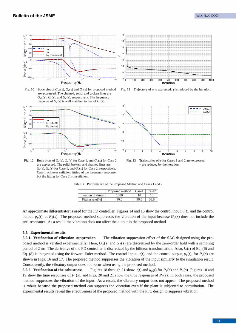
An approximate differentiator is used for the PD controller. Figures 14 and 15 show the control input,u(t), and the controloutput,yp(t), at P2(s). The proposed method suppresses the vibration of the input becauseGa(s) does not include theanti-resonance. As a result, the vibration does not affect the output in the proposed method.

5.5. Experimental results5.5.1. Verification of vibration suppression The vibration suppression effect of the SAC designed using the pro-posed method is verified experimentally. Here,Gm(s) andG f (s) are discretized by the zero-order hold with a samplingperiod of 2 ms. The derivative of the PD controller is discretized by the bilinear transformation. Also,kI (t) of Eq. (6) andEq. (8) is integrated using the forward Euler method. The control input,u(t), and the control output,yp(t), for P2(s) areshown in Figs. 16 and 17. The proposed method suppresses the vibration of the input similarly to the simulation result.Consequently, the vibratory output does not occur when using the proposed method.5.5.2. Verification of the robustness Figures 18 through 21 showu(t) andyp(t) for P1(s) andP3(s). Figures 18 and19 show the time responses ofP1(s), and Figs. 20 and 21 show the time responses ofP3(s). In both cases, the proposedmethod suppresses the vibration of the input. As a result, the vibratory output does not appear. The proposed methodis robust because the proposed method can suppress the vibration even if the plant is subjected to perturbation. Theexperimental results reveal the effectiveness of the proposed method with the PFC design to suppress vibration.

11


Fig. 14 Time history ofu(t) at P2(s) in simulation is expressed.The proposed method suppresses the vibration ofu(t)becauseGa(s) does not include the anti-resonance.

Fig. 15 Time response ofyp(t) at P2(s) in simulation is expressed.The proposed method suppresses the vibration ofyp(t).

Fig. 16 Time history ofu(t) at P2(s) in experiment is expressed.The proposed method suppresses the vibration ofu(t).

Fig. 17 Time response ofyp(t) at P2(s) in experiment is expressed.The proposed method suppresses the vibration ofyp(t).





12


6. Conclusion

The present paper proposes a PFC design method based on frequency response fitting for continuous-time SISOsystems. The conditions of frequency response fitting, the ASPR property, and the stability are derived as BMI/LMIconditions, and the BMI/LMI problem is solved using an iterative procedure. The present paper introduces the descriptionof a descriptor system instead of the state space representation. Then, the stability theorem of a descriptor system is usedin order to guarantee the ASPR property. The proposed method can treat all coefficient of the PFC as design parametersof the optimal problem because of redundancy of a descriptor system. An SAC for a mechanical vibration system isdesigned using the proposed method. The proposed method provides good frequency response fitting for PFC design.The experimental results reveal that the SAC designed using the proposed method suppresses the vibratory input andoutput, even if the plant is subjected to perturbation.

References

Adachi, S., Fundamentals of system identification, Tokyo Denki University Press (2009).(in Japanese)Chida, Y. and Nishimura, T., Discretization method of continuous-time controllers based on frequency response fitting,

SICE Journal of Control, Measurement, and System Integration, Vol.1, No.4 (2008), pp.299-306.Hino, M., Iwai, Z., Fukushima. K. and Wakamiya. R., An active vibration control by means of a simple adaptive control

method, Transactions of the Japan Society of Mechanical Engineers Series C, Vol.58, No.548 (1992), pp.1034-1040.(in Japanese)

Katayama, T., Optimal Control of Linear Systems: An Introduction to Descriptor Systems, Kindaikagaku (1999).(inJapanese)

Kyoizumi, K., Fujita, Y. and Ebihara, Y., Simple adaptive control method with automatic tuning of PFC and Its applicationto positioning control of a pneumatic servo system, Transactions of the Institute of Systems, Control and InformationEngineers, Vol.14, No.3 (2001), pp.102-109.(in Japanese)

Mizumoto, I., Ikeda, D., Hirahata, T. and Iwai, Z., Design of discrete time adaptive PID control systems with parallelfeedforward compensator, Control Engineering Practice, Vol.18, No.2 (2010), pp.168-176.

Mizumoto, I. and Iwai, Z., Recent trends on simple adaptive control (SAC), Journal of the Society of Instrument andControl Engineers, Vol.40, No.10 (2001), pp.723-728.(in Japanese)

Ohtomo, A., Iwai, Z., Nagata, M., Uchida, H. and Komera, Y., SAC (simple adaptive control) with PID and adaptivedisturbance compensation for actuator composed of artificial rubber muscles, Transactions of the Japan Society ofMechanical Engineers Series C, Vol.63, No.605 (1997), pp.166-173.(in Japanese)

Shiotsuki, T., Analysis of linear systems, Corona Publishing (2011).(in Japanese)Tanemura, M., Chida, Y. and Ikeda, Y., PFC design method using linear matrix inequality, the 56th Japan Joint Automatic

Control Conference(2013), pp.295-300.(in Japanese)Tanemura, M., Yamashiro, T., Chida, Y. and Maruyama, N., An issue of SAC for application to a plant including anti-

resonance and improvement by PFC design, Transactions of the Japan Society of Mechanical Engineers, Vol.81,No.824 (2015), pp.1-12.(in Japanese)

Uezato, E. and Ikeda M., A strict LMI condition for stability of linear descriptor systems and its application to robuststabilization, Transactions of the Society of Instrument and Control Engineers, Vol.34, No.12 (1998), pp.1854-1860.(in Japanese)

Yamashiro, T. and Chida, Y., Simple adaptive control systems design for mechanical vibration systems including antires-onance, The Society of Instrument and Control Engineers Control Division (CD-ROM), Vol.12 (2012), pp.13:40-15:40.(in Japanese)

13

Documents

Bulletin of the JSME Vol.X, No.X, XXXXBulletin of the JSME Vol.X, No.X, XXXX PFC design method for SAC based on the stability theorem of the descriptor system and frequency response