Embed Size (px)
Citation preview

BUILDING THE FULL ANNUAL CYCLE PICTURE FOR LONG-BILLED
CURLEWS: CORRELATES OF NEST SUCCESS IN THE BREEDING GROUNDS
AND SPATIAL DISTRIBUTION AND SITE FIDELITY IN THE WINTERING
GROUNDS
by
Stephanie E. Coates
A thesis
submitted in partial fulfillment
of the requirements for the degree of
Master of Science in Biology
Boise State University
May 2018

© 2018
Stephanie E. Coates
ALL RIGHTS RESERVED
BOISE STATE UNIVERSITY GRADUATE COLLEGE
DEFENSE COMMITTEE AND FINAL READING APPROVALS
of the thesis submitted by
Stephanie E. Coates
Thesis Title: Building the Full Annual Cycle Picture for Long-Billed Curlews: Correlates
of Nest Success in the Breeding Grounds and Spatial Distribution and Site
Fidelity in the Wintering Grounds
Date of Final Oral Examination: 06 February 2018
The following individuals read and discussed the thesis submitted by student Stephanie E.
Coates, and they evaluated her presentation and response to questions during the final oral
examination. They found that the student passed the final oral examination.
Jay D. Carlisle, Ph.D. Chair, Supervisory Committee
Jennifer Forbey, Ph.D. Member, Supervisory Committee
Nancy Glenn, Ph.D. Member, Supervisory Committee
The final reading approval of the thesis was granted by Jay D. Carlisle, Ph.D., Chair of the
Supervisory Committee. The thesis was approved by the Graduate College.

iv
ACKNOWLEDGEMENTS
This research was a culmination of collaborative efforts, and I am grateful for the
time and effort of so many people who made it possible. We received funding or
additional support from agencies, organizations, and other sources including the Bureau
of Land Management, United States Fish and Wildlife Service, Wyoming Game and Fish
Department, The Nature Conservancy, McDanel Land Foundation, Page Family
Foundation, MPG Ranch, Meg and Bert Raynes Wildlife Fund, Wyoming Governor’s
Big Game License Coalition, the Dan Montgomery Graduate Student Award, and many
private landowners in the Upper Green River Basin. Special thanks also to Susan Patla
from the Wyoming Game and Fish Department, Colleen Moulton from the Idaho Fish
and Game Department, Matthew McCoy and Joe Weldon from the BLM Four Rivers
Office, and Intermountain West Joint Venture and American Bird Conservancy staff for
their collaboration and insights.
I thank everyone on the curlew crew for their hard work, dedication, and for
enduring unavoidable sleep deprivation caused by hours of early-morning and late-
evening observations. Mikki Brinkmeyer, Kevin Coates, Hattie Inman, Eric Madsen, and
Jeremy Trussa all spent a season on the project and Erica Gaeta, Heather Hayes, Mikie
McDonnell, Sarah Norton, and Ben Wright spent two or more. Ben Wright’s knack for
nest-searching, efficient transmitter recovery missions, ability to independently work in a
remote field site, and willingness to devote tedious hours to identifying pixilated images
of ground cover greatly enhanced the quality of this project. I am also especially indebted

v
to Heather Hayes for her support in the field, help with project organization, leadership,
and sustaining a near-constant ice cream supply in the field house freezer.
My advisor, Jay Carlisle, balanced academic guidance, constructive feedback, and
logistical support to suit what I needed as a graduate student, and will always be a role
model for the enthusiasm he brings to his work with the natural world. I acknowledge the
helpful contributions of my committee members Jen Forbey and Nancy Glenn, who both
added to initial project concepts and manuscript revisions. Rob Miller provided study
design insight and ‘on-call’ analysis troubleshooting, Laura Bond was an invaluable
resource for statistical guidance, and Andrew Geary offered many edits and revisions to
an earlier draft of the manuscript.
Finally, the support of my family and friends made this experience possible and
enjoyable. Thank you to my neighbors in the ‘bullpen’ for providing meaningful and
mutual distractions, joining me in honoring Redbeard’s Snag, and for providing a sense
of community. In so many ways, I’m grateful for my Boise roommates over the years,
Juliette Rubin, Beck DelliCarpini, and Tina Andry, who helped me keep some sanity and
co-created a refuge in our little house. Along with many other things, the garden bounty
and cute dog pictures from my brother and sister, respectively, were much appreciated.
And lastly, I’m grateful to my parents for their support, and for providing me with so
many opportunities in life.

vi
ABSTRACT
Migratory birds face threats throughout the annual cycle, and cumulative effects
from linkages between the breeding and non-breeding grounds may impact species at the
population level. Long-billed Curlews (Numenius americanus) are a migratory shorebird
of conservation concern associated with grasslands that show breeding population
declines at some regional and local scales. Curlews exhibit high site fidelity to breeding
territories, but also spend approximately 75% of the year on the wintering grounds.
Therefore, localized population declines could indicate localized threats, in the breeding
or wintering grounds. However, little information is available regarding the spatial
distribution of curlews on the wintering grounds, especially for Mexico. Furthermore,
breeding ground studies which examine habitat selection and nest success in the context
of predator and anthropogenic pressures are lacking. We add critical information that
could help pinpoint conservation issues, including understanding limitations to nesting
success and mapping spatial distribution and habitat use patterns during the non-breeding
season. On the breeding grounds, we used a conditional logistic regression model to
compare used nest-sites to available random sites and examine habitat selection within
territories. We also studied correlates of nesting success with a generalized linear model
for 128 curlew nests at five sites in the Intermountain West. During the non-breeding
season, we attached satellite transmitters to track 21 curlews that bred in the
Intermountain West and wintered in California and Mexico and quantified 95% home
range and 50% core use size via utilization distributions created with dynamic Brownian

vii
Bridge Movement Models. For 14 individuals, we tracked multiple winter seasons and
compared inter-annual site fidelity among winter areas, sexes, and habitat type with a
Utilization Distribution Overlap Index. We documented four main wintering areas: (1)
Central Valley of California, (2) the adjoining Imperial and Mexicali Valleys of
California and Mexico, (3) the Chihuahuan Desert of inland Mexico, and (4) coastal areas
of western Mexico and the Baja Peninsula. Curlews wintering in coastal areas had
significantly smaller home ranges and fewer core use areas than inland-wintering
curlews. Home ranges in the Central Valley were larger than other inland areas, and
Central Valley females had larger home ranges than Central Valley males. Inter-annual
site fidelity for wintering curlews was high, regardless of habitat type or sex. On the
breeding grounds, curlews selected habitats for nest-sites with lower vegetation height
and lower percent cover of grasses, bare ground, and shrubs than available sites. Nest-
sites were six times more likely to have a cowpie within 50 cm than random sites. Higher
probability of nest success was associated with higher curlew density in the nesting area,
increasing percent cover of conspicuous objects such as cowpies within approximately
two meters of the nest, and – surprisingly – higher densities of American Crows and
Black-billed Magpies in the breeding area. In a separate analysis with a subset of nests (n
= 100), we found nests had higher probability of success when they were farther from
roads and perches. Given the central role of working lands to breeding curlews in much
of the Intermountain West, an understanding of limitations to nesting success in these
diverse landscapes is necessary to guide adaptive management strategies in increasingly
human-modified habitats. Similarly, foundational understanding of winter spatial ecology
is essential for understanding population declines which may be related to linkages

viii
between breeding and non-breeding seasons. Overall, these findings provide valuable
information for full annual cycle conservation and will be particularly constructive for
conservation planning once range-wide migratory connectivity is mapped.

ix
TABLE OF CONTENTS
ACKNOWLEDGEMENTS ............................................................................................... iv
ABSTRACT ....................................................................................................................... vi
LIST OF TABLES ............................................................................................................ xii
LIST OF FIGURES ......................................................................................................... xiii
LIST OF PICTURES .........................................................................................................xv
LIST OF ABBREVIATIONS .......................................................................................... xvi
INTRODUCTION: LONG-BILLED CURLEWS IN CONTEXT......................................1
CHAPTER ONE: CORRELATES OF NESTING SUCCESS AND NEST-SITE
SELECTION OF LONG-BILLED CURLEWS IN IDAHO AND WYOMING ................6
Abstract ....................................................................................................................6
Introduction ..............................................................................................................7
Study Area .............................................................................................................13
Methods..................................................................................................................19
Field Methods ............................................................................................20
Analysis Methods.......................................................................................25
Results ....................................................................................................................32
Overall Nesting Success and Causes of Failure .........................................32
Nest-site Selection .....................................................................................34
Correlates of Nest Success .........................................................................35
Predators and Disturbances ........................................................................38

x
Discussion ..............................................................................................................38
Nest-site Selection .....................................................................................40
Correlates of Nest Success .........................................................................41
Conclusions and Management Implications ..........................................................47
CHAPTER TWO: SPATIAL DISTRIBUTION AND SITE FIDELITY OF LONG-
BILLED CURLEWS WINTERING IN CALIFORNIA AND MEXICO .........................52
Abstract ..................................................................................................................52
Introduction ............................................................................................................53
Methods..................................................................................................................57
Study Area .................................................................................................57
Satellite Transmitter Attachment ...............................................................60
Statistical Analyses ....................................................................................61
Results ....................................................................................................................64
Wintering Home Range and Core Use .......................................................64
Site Fidelity: Utilization Distribution Overlap Index ................................69
Discussion ..............................................................................................................71
Home Range and Core Use Size ................................................................72
Site Fidelity ................................................................................................76
Conclusions ............................................................................................................77
COMMENTS ON INDIVIDUALITY AND ANOMALIES ............................................80
LITERATURE CITED ......................................................................................................90
APPENDIX A ..................................................................................................................106
Breeding Supplemental Information ....................................................................106
APPENDIX B ..................................................................................................................113

xi
Wintering Supplemental Information ..................................................................113

xii
LIST OF TABLES
Table 1.1 Model selection table of conditional logistic regression models which best
described selection of nest-sites used by curlews compared to random sites
within the same territory as the nest. ........................................................ 28
Table 1.2 Descriptions of parameters used in modeling Long-billed Curlew nest
success....................................................................................................... 31
Table 1.3 Candidate models for Long-billed Curlew nest success using generalized
linear models and logistic exposure links. Models within two AICc of the
top model are shown, and weights are based on this candidate set of five
models. ...................................................................................................... 32
Table 1.4 Candidate models for Long-billed Curlew nest success using generalized
linear models and logistic exposure links. Models within two AICc of the
top model are shown, and weights are based on this candidate set of four
models. ...................................................................................................... 32
Table 1.5 Long-billed Curlew nest success estimates for Idaho and Wyoming sites in
2015 and 2016. Nests with unknown fate or unknown age are not
included. .................................................................................................... 33
Table 1.6 Parameter estimates (β), standard errors, and 85% confidence intervals
from top-ranked conditional logistic regression model of nest-site
selection by Long-billed Curlews. ............................................................ 35
Table 1.7 Generalized linear model parameter estimates from binomial survival of
Long-billed Curlew nests (N = 128) modeled using a logistic exposure
link. Log-odd coefficients (β) are exponentiated as odds ratios (OR) and
85% confidence intervals (CI) are associated with the OR for
interpretation. ............................................................................................ 36
Table 1.8 Parameter estimates for correlates of Long-billed Curlew nesting success
from a subset of nests which included perch distance data (N = 100). We
used a generalized linear model with a logistic exposure link. Log-odd
coefficients (β) are exponentiated as odds ratios (OR) and 85% confidence
intervals (CI) are associated with the OR for interpretation. .................... 37

xiii
LIST OF FIGURES
Figure 1.1 A) Long-billed Curlew study sites in 2015 and 2016. B) ACEC focal areas
in southwest Idaho. C) Pahsimeroi Valley subsites in central Idaho. D)
Island Park subsites in Idaho (farthest north), the National Elk Refuge site
in Jackson, Wyoming, and Upper Green River Basin subsites near
Pinedale, Wyoming (farthest south). ........................................................ 18
Figure 1.2 Predicted probability of nest survival for parameters in selected model,
shown with 85% confidence intervals. Probability of nesting success
varied with A) curlew density in the nesting area, B) density of non-raven
corvids including American row (AMCR) and Black-billed Magpie
(BBMA) at the subsite, and C) percent cover of conspicuous objects in
immediate nest vicinity. ............................................................................ 36
Figure 1.3 Predicted probability of Long-billed Curlew nest success modeled with a
nest data set with complete perch information (N = 100) and shown with
85% confidence intervals. The model parameters included A) distance to
from the nest to the nearest perch, B) density of non-raven corvids at the
subsite, and C) distance to the nearest road. ............................................. 37
Figure 2.1 Transmitter attachment sites for Long-billed Curlews during 2013 through
2016 breeding seasons. ............................................................................. 60
Figure 2.2 High-quality location points (error radius <500m) for wintering Long-
billed Curlews tracked from Intermountain West breeding sites.............. 65
Figure 2.3 Non-breeding season a) 95% isopleth home range and b) 50% isopleth
core use size for Long-billed Curlews in the wintering California and
Mexico. ..................................................................................................... 66
Figure 2.4 Home range and core use area comparisons for Long-billed Curlews in
different non-breeding season areas; two-letter codes indicate letters on
alpha flags for each bird. ........................................................................... 67
Figure 2.5 Size of 95% isopleth home range for Long-billed Curlews a) wintering in
coastal versus inland areas and b) comparing home range size of Central
Valley females to Central Valley males. Home range size was
significantly greater for curlews wintering inland and for Central Valley
females, than for coastally wintering birds and Central Valley males. .... 68

xiv
Figure 2.6 Number of distinct core use areas for Long-billed Curlews wintering in
coastal and inland habitats. ....................................................................... 68
Figure 2.7 Inter-annual UDOI for Long-billed Curlews in California and Mexico
wintering areas. For individuals tracked three seasons, we used the
average of consecutive seasons for analyses. ........................................... 70
Figure 2.8 Average inter-annual UDOI scores for a) coastal and inland habitats and
b) female and male Long-billed Curlews. For individuals tracked three
years, we used the average of UDOIs from consecutive years. All UDOI
values were greater than one (dotted line), indicating a high degree of
home range overlap between years. .......................................................... 70
Figure 2.9 Inter-annual UDOI for Long-billed Curlews grouped by sex and habitat
type. For individuals tracked three years, we used the average of
consecutive years. No male curlews were tracked for more than one year
in coastal areas. ......................................................................................... 71
xv
LIST OF PICTURES
Picture 1. Blue-green curlew egg coloration with larger dappled maculation. Flat
Ranch, Island Park, ID. May 2015. Photo by Hattie Inman. .................... 82
Picture 2. Blue-green curlew egg coloration with uneven maculation. ACEC,
southwest ID. May 2015. Photo by Stephanie Coates. ............................. 83
Picture 3. Brownish-green curlew egg coloration with fine, evenly distributed flecks.
Big Creek, Pahsimeroi Valley, ID. May 2017. Photo by Ben Wright. ..... 83
Picture 4. Tan curlew egg coloration, with one egg pipping. ACEC, southwest, ID.
June 2016. Photo by Stephanie Coates. .................................................... 84
Picture 5. Curlew egg coloration with pink hues. National Elk Refuge, Jackson, WY.
May 2016. Photo by Erica Gaeta. ............................................................. 84
Picture 6. Three-egg clutch of a curlew with a wood debris ‘spacer’. ACEC,
southwest ID. May 2015. Photo by Stephanie Coates. ............................. 86
Picture 7. Three-egg clutch of a curlew with a cow dung debris ‘spacer’. Big Creek,
Pahsimeroi Valley, ID. May 2017. Photo by Ben Wright. ....................... 86
Picture 8. Dent in a Long-billed Curlew egg. ACEC, southwest ID. May 2016. Photo
by Stephanie Coates. ................................................................................. 87
Picture 9. Badger burrow which a juvenile curlew entered and remained for
approximately 15 minutes. ACEC, southwest ID. July 2016. Photo by
Stephanie Coates. ...................................................................................... 88

xvi
LIST OF ABBREVIATIONS
BSU Boise State University
GC Graduate College
TDC Thesis and Dissertation Coordinator

1
INTRODUCTION: LONG-BILLED CURLEWS IN CONTEXT
Migratory grassland birds face threats in all parts of their annual cycle (Sillett and
Holmes 2002, Webster et al. 2002, Newton 2004, Holmes 2007), but timing and intensity
of negative pressures may vary by species and across populations. Consequently,
conservation efforts for such species need to consider reproductive success, winter
mortality, as well as migration risks and more subtle indirect threats (Sutherland 1996,
Norris 2005). Foundational information for many migratory birds, such as the location of
key wintering areas, spatial use and distribution in those areas, and links between
segments of the annual cycle remains unknown, however. A better understanding of the
complete annual cycle is important for identifying causal factors of declining populations
because habitat quality and fine-scale conditions experienced by wildlife in one stage of
the annual cycle may induce carry-over effects, where fitness consequences emerge in
subsequent portions (Norris and Taylor 2006, Norris and Marra 2007, Harrison et al.
2011). In addition, although the amount of research taking place on breeding grounds
generally outweighs efforts in other portions of the annual cycle (Faaborg et al. 2010), for
many species important limitations are occurring on the breeding grounds and still
warrant further research (Sherry and Holmes 1995). Further identifying limitations to
reproductive success, especially in the context of threats at different scales, is a critical
component of developing effective conservation plans for many declining bird species
(Orians and Wittenberger 1991). Equally important is understanding spatial distribution

2
throughout the range of a species because both areas of research provide a framework for
identifying habitat requirements and can pinpoint threats to a population.
Grassland birds experienced steeper population declines from 1966 to 2015 than
any other avian group in North America (Sauer et al. 2017). The current conservation
status designated by the State of the Birds Watchlist for the group is ‘Steep Declines’,
one level below the most critical ‘In Crisis’ category. Notably, there have been 70%
population losses since 1970 of grassland species migrating between the Great Plains and
the Chihauhuan Desert of Mexico (NABCI 2016). North American grasslands have
undergone rapid and drastic habitat changes in a similar period. Once comprising half of
the lower 48 states, conversion to agriculture or rangeland, invasion by non-native
vegetation (Steidl et al. 2013), development, and anthropogenic disturbances have led to
the loss or conversion of approximately 28% of all grassland from 1850 to 1990 (Conner
et al. 2001). In the Great Plains, approximately half of grasslands remain intact, with 8%
converted to agriculture between 2009 and 2017 alone (Plowprint Report 2017). Since
1950, more than a third of the losses represent conversion to habitat types other than
agriculture (Conner et al. 2001). Grassland alterations may catalyze population-level
changes in avian communities by affecting reproductive success. Nesting success for
some grassland breeders is influenced by vegetation structure and composition (Winter et
al. 2005), and habitat conditions are often correlated with nesting success because they
are associated with foraging resource quality (Pärt 2001), predator density (Whittingham
and Evans 2004), and anthropogenic disturbances (Carney and Sydeman 1999, Beale and
Monaghan 2004).
3
The Numeniini are a tribe of wading shorebirds globally recognized as imperiled
and in need of collaborative conservation action; of 13 species, seven are critically
endangered, endangered, or near threatened (Pearce-Higgins et al. 2017). Numeniini share
life history traits which cumulatively increase susceptibility to extinction, including long-
distance migrations (Sanderson et al. 2006), late age of reproductive maturity, and low
fecundity (Piersma and Baker 2000). One member of the Numeniini are long-billed
Curlews (Numenius americanus), a migratory shorebird of conservation concern that
breed in grasslands, pastures, some agricultural croplands across the Intermountain West
and much of the Great Plains in the U.S. and Canada (Dugger and Dugger 2002, Fellows
and Jones 2009). Two subspecies are sometimes recognized: the larger-bodied N. a.
americanus in more southern parts of the breeding range, and the northern, smaller-
bodied N. a. parvus (Dugger and Dugger 2002). In relation to some Numeniini, curlews
have more generalist habitat requirements, selectively occupying a range of grasslands,
including pastures, rangelands, wetlands, and some types of agriculture (Saalfeld et al.
2010), a characteristic which may have shielded curlews so far from more serious
population declines.
On the breeding grounds, Breeding Bird Surveys (BBS) from 1966 to 2015
suggest curlews have range-wide population stability, where population decreases in
some portions of the range are balanced by population increases in others (Sauer et al.
2017). However, while BBS provides the most thorough account of long-term relative
population trends available for curlews, population estimates for the species may be
unreliable because data are sparse, detections are infrequent in many states, and surveys
are conducted during or after incubation – after the display period when curlews are most

4
conspicuous (Stanley and Skagen 2007, Fellows and Jones 2009, Sauer et al. 2017). State
Wildlife Action Plans in 16 states in which curlews occur list them as a Species of
Greatest Conservation Need (USGS SWAP 2017). Federally, curlews are designated a
Bird Species of Conservation Concern by the USFWS, ‘sensitive’ by the BLM in most
breeding states, and ‘highly imperiled’ by the U.S. Shorebird Conservation Plan (Brown
et al. 2001). Internationally, the Committee on the Status of Endangered Wildlife in
Canada considers curlews of ‘Special Concern’ (COSEWIC 2002, 2011). These concerns
stem from uncertainty in population status as well as significant habitat alterations and
other potential threats range-wide.
Although curlew populations occur in a variety of grassland habitats, past studies
indicate that individuals have high site fidelity to breeding areas (Redmond and Jenni
1982), which may limit plasticity for home range shifts following habitat degradation or
loss. Further limiting options for curlews displaced by habitat loss, the habitat in areas to
which they are displaced may also be degraded or disappearing. For example, in a key
curlew wintering area, the Central Valley of California, more than 30% percent of
wetlands were lost between 1939 and the mid 1980’s (Frayer et al. 1989). Wintering
ground site fidelity research is limited but has shown variation at different spatial scales;
high fidelity to winter home ranges, but lower fidelity to small-scale foraging patches
(Sesser 2013). Habitat loss and degradation is widespread, non-discriminatory, and a
concern even for generalist species, such as the Long-billed Curlew.
In 2009 the US Fish and Wildlife service published a conservation action plan for
Long-billed Curlews (Fellows and Jones 2009). The outlined conservation actions fall
into four groups: 1) population monitoring and assessment; 2) habitat assessment and

5
management; 3) research; and 4) education and outreach. Since the publication of the
plan, curlew research has filled existing gaps in each of these categories, especially with
regards to assessing nesting success and breeding habitat in areas where information was
lacking (Hartman and Oring 2009, Gregory et al. 2011, 2012), tracking migratory routes
(Page et al. 2014), mapping wintering range and habitat (Sesser 2013, Page et al. 2014,
Kerstupp et al. 2015) and studying wintering ecology (Navedo et al. 2012, Shurford et al.
2013, Kerstupp et al. 2015). Our research addressed several of the identified knowledge
gaps, but also added components beyond the scope of the plan. Specifically, we added
baseline and comparative population density and nesting success information for many
sites in the Intermountain West and gave context to nesting success by assessing the role
of habitat, potential communal defense, nest-site selection, predator density, and
anthropogenic features. We also assessed wintering range locations, and spatial
distribution patterns and site-fidelity in those ranges. Our research fueled community
education and outreach through public presentations, volunteer involvement, curlew
naming contests for tagged birds, a live-stream satellite tracking map, and a ‘Curlews in
the Classroom’ program delivered to K-12 students in southwest Idaho. Through this
public engagement we aimed to reduce an identified threat to curlews in southwest Idaho,
illegal shooting, and to share knowledge we gained through collaborative efforts.

6
CHAPTER ONE: CORRELATES OF NESTING SUCCESS AND NEST-SITE
SELECTION OF LONG-BILLED CURLEWS IN IDAHO AND WYOMING
Abstract
Grassland birds have experienced steeper population declines between 1966 and
2015 than any other bird group on the North American continent, and migratory
grassland birds may face threats in all portions of their annual cycle. Long-billed Curlews
(Numenius americanus) are a large, grasslands-breeding shorebird of conservation
concern with identified population declines in regional and localized portions of their
breeding range. Much of the landscape used by curlews is considered working land,
including agriculture, rangelands, and pastures. Curlews are long-lived and exhibit high
fidelity for breeding ground territories, but also spend three-quarters of the year on the
wintering grounds. Thus, localized population declines could indicate localized threats on
the breeding or wintering grounds. Nesting success is one critical juncture of the annual
cycle at which curlews may face limitations from nest predators and anthropogenic
disturbance. Nest depredation threats may be countered through selection of nest-site
habitat which increases concealment, or advanced warning of predators provided by
higher densities of conspecifics for communal defense. Some anthropogenic features,
such as roads, fences, and other structures, may impose direct or indirect risks to curlew
nests, and similarly may be countered by selection of nest-site habitat. We compared
nest-sites versus random sites within the same territory to examine nest-site selection, and
modeled correlates of nesting success for 128 curlew nests at 5 Intermountain West sites.

7
Nest-sites were 6 times more likely than random sites to be adjacent to conspicuous
objects. Additionally, curlews selected nest-sites with shorter vegetation, and less bare
ground, grass, and shrub cover, than at random sites within territories. We found nest
success varied widely among sites and ranged from 12 to 40% in a season. Higher nest
success probability was associated with higher curlew densities in the area, greater
percent cover of conspicuous objects near the nest, and, surprisingly, higher densities of
non-raven corvids at the site. In a second analysis, we also found increased probability of
nesting success with increased distance between nests and the nearest potential perch.
Given the central role of working lands to birds in much of the Intermountain West,
understanding limitations to nesting success in these diverse landscapes is necessary to
guide adaptive management strategies in increasingly human-modified habitats.
Introduction
Full annual cycle research of migratory birds is critical for conservation because
species may face threats on the breeding grounds, during migration, or on the non-
breeding grounds, and the timing and intensity of threats potentially vary across
populations (Sillett and Holmes 2002, Webster et al. 2002, Newton 2004, Holmes 2007).
Consequently, conservation efforts for such species need to consider reproductive
success, winter mortality, as well as migration risks and subtle indirect threats such as
carry-over effects (Sutherland 1996, Norris 2005). The amount of research taking place
on breeding grounds generally outweighs efforts in other portions of the annual cycle
(Faaborg et al. 2010) where more work is needed. However, for many species, important
limitations are occurring on the breeding grounds that also warrant further research
(Sherry and Holmes 1995). Identifying limitations to reproductive and nesting success,

8
especially in the context of threats at different spatial scales, will be a critical component
of developing effective conservation plans for many declining grassland bird species
(Orians and Wittenberger 1991).
Long-billed Curlews (Numenius americanus) are a shorebird of conservation
concern that breed in grasslands, pastures, and some agricultural croplands across the
Intermountain West and much of the Great Plains in the U.S. and Canada (Dugger and
Dugger 2002, Fellows and Jones 2009). Based on population estimates from the Breeding
Bird Survey (BBS), increasing curlew numbers in some areas may be balancing
population declines in other areas, creating range-wide stability (Sauer et al. 2017).
Concerns with the BBS curlew population estimates such as wide confidence intervals
due to sometimes sparse data, infrequent detections in many states, and surveys
conducted during or after incubation when curlews are least conspicuous (Stanley and
Skagen 2007, Fellows and Jones 2009, Sauer et al. 2011), has prompted other range-wide
population assessments for the species. These more recent estimates also suggest that,
across the entire range of the species, curlew numbers are likely not as low as previously
thought (Stanley and Skagen 2007, Fellows and Jones 2009). However, steep declines
recorded in some breeding areas (Pollock et al. 2014) as well as significant habitat
alterations range-wide (see Fellows and Jones 2009) are cause for concern and curlews
continue to be listed as a Species of Greatest Conservation Need by State Wildlife Action
Plans in 16 states across the western and central United States – most of the states in
which they breed (USGS SWAP 2017). Furthermore, several characteristics unique to
curlew life history also stress the need for greater understanding of the threats for curlews
at breeding grounds. Specifically, curlew pairs have strong breeding territory fidelity,

9
with males exhibiting high natal philopatry, and females only occasionally moving to
new breeding territories, likely in cases where nesting attempts the previous year failed
(Redmond and Jenni 1982). Therefore, negative population trends from the breeding
grounds suggest adult mortality, low nesting success, or low recruitment rather than
emigration by adults. Furthermore, declining local abundance for long-lived species may
be a more reliable early indicator of overall population decline than range constriction
through site occupancy (Méndez et al. 2017). Unless the age structure is known in the
population of a long-lived species, there may be a lag-time in the detection of declining
populations (Redmond and Jenni 1986). Finally, curlews also use communal defense
strategies to deter predators from nesting areas (Pampush 1981), and loss of population
density in breeding areas could amplify nest failures caused by predators, creating a
negative feedback loop.
The decline of curlew numbers has generally been attributed to extensive habitat
loss, degradation, and fragmentation of across the grasslands of North America where
curlews nest (Fellows and Jones 2009, Conner et al. 2001). Alterations of grassland may
catalyze population-level changes in avian communities by affecting reproductive
success. Nesting success for some grassland breeders is influenced by vegetation
structure and composition (Winter et al. 2005), and habitat conditions are often correlated
with nesting success because they are associated with foraging resource quality (Pärt
2001), predator density (Whittingham and Evans 2004), and anthropogenic disturbances
(Carney and Sydeman 1999, Beale and Monaghan 2004).
Habitat conditions related to curlew nesting sites have been heavily studied
(reviewed in Fellows and Jones 2009), but we propose two reasons why further research

10
is needed. First, existing habitat selection studies have reported contradictory findings,
which may be a product of formerly more common ‘used’ vs. ‘unused’ site comparison
methodologies (Jones 2001), or inconsistent ground cover estimates (Booth et al. 2015).
For example, while Cochran and Anderson (1987) found nest-sites had more grass cover
and less bare ground than in surrounding fields, Pampush and Anthony (1993) found bare
ground was a ‘spurious’ predictor of used and unused sites, and Paton and Dalton (1994)
found curlews preferred to nest near, though not directly on, patches of bare ground.
Jenni et al. (1981) suggested that vegetation structure may be more important than
composition for curlew habitat selection, and this may be similar for nest-site selection.
Male curlews defend breeding territories from 6 to 14 ha in size and the pair selects a
location for their nest within their breeding territory (Dugger and Dugger 2002).
Comparing nest-sites to ‘unused’ sites may not be an adequate measure of nest-site
selection because habitat outside of the territory is not technically available to the curlew
pair (Jones 2001).
Second, research efforts to date have rarely evaluated how habitat variables relate
to nest success (but see Clarke 2006 and Gregory et al. 2011), and none have evaluated a
comprehensive list of biologically meaningful variables at multiple scales. Many studies
have identified and described habitat characteristics at curlew nest-sites, defined as the
habitat immediately surrounding the nest (McCallum et al. 1977, King 1978, Allen 1980,
Jenni et al 1981, Pampush 1981, Redmond 1986, Pampush and Anthony 1993, Paton and
Dalton 1994, Saalfeld et al. 2010, Blake 2013). Fewer have examined associations
between even coarser-scale habitat conditions (e.g. ‘annual grassland’ or ‘grazed field’)
and nest success (Cochran and Anderson 1987, Pampush and Anthony 1993). Curlew

11
studies which have examined nest success in relation to nest-site habitat variables focused
on vegetation height and ground cover composition. Clarke (2006) found a positive
association between vegetation height and nest success, despite curlews apparently
selecting nest-sites with shorter vegetation than random sites in the same breeding area.
Again, it should be noted that these random sites may not have been truly ‘available’,
because they were not necessarily within the territory of the nesting curlews. In contrast,
Gregory et al. (2011) found a negative association between nest success and vegetation
height. The effect of forb cover on nest success was also incongruous in these two studies
and neither study provided a potential mechanism for the influence of forb cover versus
other vegetative cover on nesting success. Given that the average success rate of curlew
nests is reported at 31-69 percent (Pampush and Anthony 1993, Hartman and Oring
2009) and may range widely between years and within the same habitat type, it is not
enough to simply know which habitats are associated with higher nest success. Instead,
research that explains the link between nest success and biologically-relevant conditions
across multiple scales including habitat at the nest-site, is needed to more fully guide
conservation efforts for declining bird species (Gregory et al. 2011).
Although many habitat factors may influence nest success, the most common
direct cause of nest failure is predation (Ricklefs 1969), and ground-nesting grassland
birds are especially susceptible to predation (Best et al. 1997). Along with cryptic
coloration (Wallace 1889), birds may minimize predation risk through nesting in areas
with high density of conspecifics to facilitate communal defense (Macdonald and Bolton
2008), or by selection of nest-sites based on desirable habitat features, such as vegetation
structure (Winter 2005). However, habitat selection, particularly at the nest-site level, is

12
nuanced. For example, nests which are situated in denser vegetation may be more well-
concealed from predators, but if the vegetation is too tall it may hinder the visibility an
incubating bird has of the surroundings. Visibility of nest surroundings may allow
advanced warning of approaching predators and facilitate recruitment of conspecifics to
fend off threats (Götmark et al. 1995). Furthermore, some species exhibit adaptive
plasticity in response to perceived predation pressure – selecting nest-sites with higher
concealment when the predation pressure warrants (Forstmeier and Weiss 2004). In
relatively homogenous environments such as grasslands, nest-sites surrounded by similar
habitat could decrease search-efficiency by predators (Martin and Roper 1988). These
fine balances suggest habitat comparisons for nest-sites may be scale-dependent, and
subtle. Furthermore, habitat selection of nest-sites by most bird species only indirectly
mediates depredation threats. Concurrent data regarding common predator densities (e.g.,
badgers [Taxidea taxus], coyotes [Canus latrans], and corvids; Redmond and Jenni 1986,
Pampush and Anthony 1993), anthropogenic features which may pose threats (e.g., roads
and grazing; Pollock et al. 2014), and density of conspecifics (Macdonald and Bolton
2008) is required to obtain a more detailed picture of this complex, and potentially
limiting portion of the annual cycle.
We conducted a wide-scale study of curlew nesting success, recognizing the
interconnectedness of habitat selection at nest-sites and external drivers of nesting
success. Two of our sites were previously studied, one in southwest Idaho (1977-1979;
Redmond and Jenni 1986) and the other in western Wyoming (1982; Cochran and
Anderson 1987), and we compared current and historical estimates of curlew density and
nest success at these sites. We also included three other sites which lacked baseline data

13
on nesting success but provided a diversity of grassland habitats and included private and
federal government ownership. We compared used nest-sites to random sites which were
available within the same territory to examine nest-site selection, and further explored
how finer-scale nest habitat characteristics and broader-scale site characteristics were
associated with nest survival. Our research builds on and clarifies past curlew studies on
breeding-grounds by measuring densities of curlews and known predators in nesting
areas, as well as considering a more comprehensive evaluation of natural and
anthropogenic habitat features.
Based on our existing knowledge of curlew biology we predicted that 1) nesting
success would be lower in breeding areas that had higher predator density, 2) curlews in
higher density nesting areas would have greater nesting success potentially due to the
greater capacity for communal defense, and 3) curlews with nest-sites closer to
anthropogenic features such as roads would have lower nesting success. We also
predicted that curlews selectively choose nest-sites near conspicuous objects, with greater
visibility from the nest (i.e., lower vegetation height), and with higher concealment via
denser vegetation or visual obstruction from surrounding habitat features such as
hummocks. We examined these variables in the Intermountain West with a natural
experiment.
Study Area
We conducted field work from April to July in 2015 and 2016 at breeding sites
located in the Intermountain West region of Idaho (3 sites) and Wyoming (2 sites). At
several breeding sites we worked within geographically distinct ‘subsites’, which were
not contiguous. In southwest Idaho we worked within two nesting areas where curlews

14
were clustered, but the habitat was not geographically distinct. We described these as
‘focal areas’ (see Appendix A.1 for site and focal area summary table). The sites, subsites
and further details included:
1. The Long-billed Curlew Habitat Area of Critical Environmental Concern
(ACEC), including two focal areas, near the town of Emmett, southwest Idaho
(Figs. 1.1A & 1.1B).
2. The Pahsimeroi Valley near the town of May, central Idaho (Figs. 1.1A & 1.1C).
3. The Nature Conservancy’s Flat Ranch and the Shotgun Valley in the Island Park
area near West Yellowstone and Island Park area in eastern Idaho (Figs. 1.1A &
1.1D).
4. Upper Green River Basin at Horse Creek and New Fork near the city of Pinedale,
western Wyoming (Figs. 1.1A & 1.1D).
5. The National Elk Refuge, Jackson, western Wyoming (Figs. 1.1A & 1.1D).
The Long-billed Curlew Habitat Area of Critical Environmental Concern,
hereafter the ‘ACEC’, was considered an important curlew breeding area after intensive
research in the late 1970s revealed a dense breeding population (Redmond and Jenni
1986). The ACEC was managed by the Bureau of Land Management (BLM) and is an
arid upland, rolling grassland (~2,400’ elevation) dominated by invasive annual grasses
including cheatgrass (Bromus tectorum), the invasive forb tumble mustard (Sysimbrium
altissimum), as well as some native grasses, especially Sandberg’s bluegrass (Poa
segunda). In the pre-dust bowl era before fires and human alteration converted the area to
annual grasslands, the habitat was likely composed of mostly sagebrush with grassland

15
pockets (Jenni et al. 1981). Public use of the land included recreational shooting, cattle
grazing, and off-highway vehicle (OHV) recreation. Grazing by cattle or sheep typically
occurred in spring and summer, and animals were sometimes shifted between pastures
during the peak of the curlew breeding season. In the 1970s, there was more grazing by
sheep than cattle (Bicak et al. 1982), but the proportions have shifted and, in the study
years we only observed cattle grazing in focal curlew nesting areas. Results from
historical curlew research were available for comparison with current research (i.e., Jenni
et al. 1981, Bicak et al. 1982, Redmond and Jenni 1982, 1986). We focused nest
searching in two areas with higher curlew density than surrounding areas; focal nesting
areas we named Emmett A and Emmett B. Both focal areas were similar in terms of
abundant ground squirrels and human recreational use, but ease of access by the public
varied. Emmett B was easily accessed via a paved road and frequently used for OHV
activities, while Emmett A received less use because accessing most of the area required
more travel time via an unimproved dirt road and passing through several barbed wire
cattle pasture gates.
Between the Lost River and the Lemhi mountain ranges, the Pahsimeroi Valley
site (~5,100’ elevation) is comprised of two small private parcels each of which we
designated a subsite of the Pahsimeroi: Goldburg and Big Creek. Crops irrigated by
center-pivots were the dominant vegetation at Big Creek, and Goldburg was a sub-
irrigated wet meadow which abuts native sagebrush habitat as well as a separately-owned
agricultural field. The wet meadow habitat had diverse grasses, sedges, rushes and forbs,
but Juncus sp., Timothy (Phleum pratense), clover (Trifolium spp.) and dandelion

16
(Taraxacum officinale.) were most abundant. Cattle grazing was restricted to late
summer, after the curlew nesting season.
In the Island Park area of eastern Idaho, we conducted nest searching and
monitoring in two subsite locations. The first, the Nature Conservancy’s Flat Ranch
(~6,300’ elevation), had a flat, wet meadow habitat similar to the Pahsimeroi Valley.
Grazing was carefully managed with quick rotations among fenced pastures and timed to
avoid overlapping with the curlew nesting season. Flood-irrigation also occurred after the
nesting season had concluded. Public access was limited, but people were permitted to
cross through part of the study area on a dirt two track to fish at a nearby creek. A second
area southwest of Flat Ranch called the Shotgun Valley, and had mixed land ownership
(BLM, state, and private ownership) and different habitat types that included mostly
sagebrush with scattered pockets of wet grassland and cattle grazing occurred on portions
of the subsite.
The subsites within the Upper Green River Basin, named Horse Creek and New
Fork, were privately owned, and we accessed each parcel with landowner permission.
The landscape in the monitored area was characterized by flat topography, high-elevation
(~7,200’), flood-irrigated pastures and hayfields composed of diverse grasses, forbs, and
rushes. Timothy (Phleum pratense), wire grass (Jucus balticus), sedges (Carex spp.), and
red-top (Agrostis palustris) were the most abundant vegetation species, with willows
(Salix spp.) and other shrubs often at the edges of fields and along riparian corridors. In
early spring, landowners drug their fields to break up cowpies, and cattle grazing was
concurrent with curlew nesting in some pastures. These two study sites overlapped the

17
study area boundaries of historical research by Cochrane and Anderson (1987) and
further study site details can be found therein.
The National Elk Refuge in Jackson, Wyoming is a high elevation valley
(~6,400’) bounded by the Teton Mountains to the northwest and the Gros Ventre
Wilderness area to the east. The land was managed by the U.S. Fish and Wildlife Service,
and public access was restricted to roads only. The refuge supported large numbers of
wintering elk and other ungulates through added irrigation in the summer and
supplemental feeding. Primary vegetation in curlew nesting areas included Sandberg’s
bluegrass (Poa secunda), needle-and-thread grass (Stipa comata), crested wheatgrass
(Agropyron sp.), spiny phlox (Phlox hoodii), and green rabbitbrush (Chrysothamnus
vicidoflorus).

18
Figure 1.1 A) Long-billed Curlew study sites in 2015 and 2016. B) ACEC focal
areas in southwest Idaho. C) Pahsimeroi Valley subsites in central Idaho. D) Island
Park subsites in Idaho (farthest north), the National Elk Refuge site in Jackson,
Wyoming, and Upper Green River Basin subsites near Pinedale, Wyoming (farthest
south).

19
Methods
We measured nest-site selection and nest success variables at several different
scales. The smallest scale, the nest-site, included the habitat within approximately 10 m
or less of the nest cup. Nest-sites were within the territories of curlew pairs which are
established early in the season by males through undulating flight displays and agonistic
behaviors (Allen 1980, Jenni et al. 1981). While females incubate during the day, males
typically remain in their territories foraging, preening, or standing guard. Territory
boundaries are somewhat loose and the size may vary from approximately 6 to 14 ha
(Allen 1980, Jenni et al. 1981). We were reasonably confident that through behaviorally-
based nest searching and extended observation, we could discern approximate territory
boundaries. At the next spatial level, we delineated ‘focal nesting areas’ where territories
were clumped closely together. Subsites included larger areas of land to which we had
research access. We made the distinction between subsites and focal nesting areas
specifically when curlew distribution was unequal across the span of a subsite and it
would have been inefficient to conduct nest-searching across the low-density areas of the
subsite. When curlews were evenly distributed throughout the subsite we did not
delineate separate ‘focal nesting areas’, as there was no need. Finally, we nested subsites
within broader study sites, which were simply areas that were relatively distinct
geographically (e.g., the Upper Green River Basin), and could be accessed on a daily
basis by the same crew.

20
Field Methods
Early-season Curlew Point Counts
At the start of the breeding season, we conducted standardized point counts across
all study areas. During this time, male curlews perform territory displays and incubation
has not been initiated. We repeated historical road routes when possible, expanded
surveys to include off-road points, and plotted new road transects in many areas. We
spaced points a minimum of 800 m apart, and traveled between road points in a vehicle,
and between off-road points on foot. Beginning 30 minutes after sunrise, two observers
recorded the distance to curlews detected aurally or visually during 5-minute counts at
designated points as in Jones et al. (2003). Both observers scanned for curlews and one
observer recorded data. The role of data recorder alternated at each point. Observers
recorded distance to the curlew, sex of the bird, the number of curlews detected, behavior
or status (e.g., flying over, displaying, etc.), wind intensity using the Beaufort scale, and
temperature at the start and end of the survey. We used point count observations,
particularly of pairs, to focus nest-searching efforts and later to estimate curlew density in
specific subsites, or focal areas within sites where we located nests.
Surveying Predators and Anthropogenic Disturbance
We used distance sampling to assess relative levels of predator density and
anthropogenic disturbance among nesting areas. We followed a stratified random
transects design and placed transects at a density of approximately one transect per
square kilometer. We separated parallel transect lines by a minimum of 800 meters to
reduce the likelihood of counting a predator or disturbance from more than one transect.
We repeated each 500-m-long transect three times per season, with varied timing (i.e., a

21
transect was not surveyed in the morning during all three visits). We paced walking speed
on transects for a minimum duration of 30 minutes, and recorded duration as a control
variable. We recorded the distance and sighting angle to any animal that was a potential
predator for curlew nests or adults and to any anthropogenic activity or feature that could
be a potential disturbance for curlews (e.g., OHV recreationists and trails target shooting,
vehicular traffic roads). We measured distance with a rangefinder, and used a compass to
calculate sighting angle, defined as the difference in degrees from the transect line
bearing and the sighted predator or anthropogenic disturbance. In addition, we recorded
inanimate predator and anthropogenic disturbance signs such as crushed vegetation
indicating off-road travel, abandoned shooting targets, and fresh badger burrows.
Nest-site Habitat
We standardized timing of habitat data collection by visiting nests sites
approximately one week (7 ± 0.35 SE days) post-hatching, or a week after projected
hatch date if the nest failed, to minimize measurement bias introduced by temporal
factors (McConnell et al. 2017). Within the same territory as the nest and during the same
visit, we also assessed the habitat parameters at four random sites selected by randomized
compass bearings and distances. We restricted the maximum distance from the nest cup
to any random site to 125 m, and re-selected random sites if the selected site appeared to
be outside the territory boundaries, or in a location were nesting was not possible (e.g., in
a river) because we deemed those locations ‘unavailable’ as nest-sites. At nest-sites and
random sites, we measured the distance to nearest anthropogenic features and distances to
potential perches for avian predators with a rangefinder.

22
At the nest-site and random sites, the habitat parameters we measured in situ
included effective visible height, concealment, the number of cowpies in a 3 m radius,
and the distance to the nearest cowpie from the center of the nest cup or site. The ability
to detect approaching predators while incubating could be advantageous (Allen 1980) and
visibility from a nest-site is affected by vegetation height as well as topography. Thus, for
a biologically meaningful quantification of visibility, we measured the height at which a
white board set 10 m away from the nest cup was 90% obscured, when viewed from the
eye-level of an incubating curlew (approximately 25 cm). This is a slight modification of
Wiens (1973) ‘effective height’ where the white board is viewed from a height of 1 m,
and similar to the protocol used by Bicak (1982) in a curlew grazing study. We termed
this measurement ‘effective visible height’ and recorded the value in each cardinal
direction. To assess the relative level of concealment a curlew would be afforded while
incubating, we used a 20 x 25 cm red-and-white checkered cube (20 4 x 4 cm squares per
side), viewed from 10 m away and 75 cm high (approximately coyote eye-level) in each
cardinal direction. If a square was ≥50% visible, we did not consider it concealed. We
prepared the data for analysis by averaging effective visible height measurements from
each cardinal direction and dividing the sum of concealed squares on each face of the
cube by the total number of squares to create one measurement of effective visible height
and percent concealed, per nest-site or random site.
Visual estimation of percent ground-cover can be inaccurate and difficult to
standardize among a large crew. To reduce observer bias in percent cover estimates, we
digitized the process using the program SamplePoint (Booth et al. 2006), and quantified
percent cover of vegetation functional groups. While conducting nest habitat

23
measurements, we used a 2 m tall pole and a downward-facing camera mounted at the
end of a 75 cm boom which was parallel to the ground to take pictures on each side of the
nest and random sites. In SamplePoint, we calculated percent cover using either 84- or
100-point grids overlaid on each image. Two individuals, Coates and Wright, conducted
the entire analysis and trained for consistent identification of the following categories:
bare ground, grass, forb, shrub, litter/debris, conspicuous object, water, equipment, or
unknown. The conspicuous objects category was a combination of points marked either
as cowpies or other conspicuous objects (e.g., large rocks). This designation was
necessary for analyses because aerial concealment could be provided by objects other
than cowpies, and because not all study sites had cattle present. With SamplePoint
results, we divided the number of grid points identified as a given category by the total
number of identifiable grid points in the image to calculate percent cover of vegetation
groups.
Depending on latitude and elevation, the breeding season at each site began at
different times. Therefore, initiation date relative to the beginning of the breeding season
was a parameter of higher interest than Julian calendar dates. We examined the effect of
initiation date relative to site green-up date, using green-up date as a proxy for the start of
the breeding season. We used long-term (2000−2013) MODIS Phenological Parameters
produced by the USDA Forest Service to determine a coarse estimate of the median
green-up date window at each breeding subsite (ForWarn 2017) and then selected the
midpoint of the date range window as green-up date for the breeding subsite.

24
Monitoring Nest Survival
Curlews are cryptic nesters and spend minimal time preparing a cupped scrape on
the ground where they will usually lay four eggs. The egg-laying stage takes 4.5 days
(~1.5 days between eggs), followed by an incubation stage that lasts approximately 28-29
days from the time the last egg is laid, with females incubating during the day and males
during the night (Pampush and Anthony 1993, Dugger and Dugger 2002, Hartman 2008).
We capitalized on behavioral cues, particularly incubation switches, to locate nests. On
the initial visit after locating a nest, we floated eggs to estimate age (Liebezeit 2007) and
minimize the number and proximity of future visits. Every three to five days thereafter
we viewed nests from the farthest vantage point from which we could confirm status. We
increased visitation frequency to one check per day in the days leading up to predicted
hatch date. If at least one egg hatched, we considered a nest successful.
When nests failed, we immediately and systematically searched the area in a 50 m
radius from the nest for egg remains and predator sign. We conservatively assigned an
avian or mammalian predator identification, but often avoided more specific
identification because of considerable overlap among species in observable sign left by
predators (Larivière 1999, Pietz and Granfors 2000). For example, digging at the nest
bowl and cached eggs is characteristic of mammalian depredation, and missing eggs
could be attributed to Common Ravens (Corvus corax), coyotes, or a number of other
predators that are known to take eggs whole (Larivière 1999).

25
Analysis Methods
Quantifying Curlew Density in Focal Nesting Areas
We used the R package ‘Distance’ (Miller 2017, R Core Team 2017) to calculate
curlew density in subsites and focal nesting areas. We designated points from early
season point counts as being within a subsite or focal nesting area if a monitored nest
which was included in the analysis was within approximately 1600 meters of a point
count location. This was a conservative approach and allowed inclusion of more points
for density estimates, but may have underestimated density in nesting areas where
curlews are more tightly clustered. For the analyses, we included all observations except
those in which the curlews did not appear to be in a home territory, such as ‘fly-over’
individuals, to avoid over-estimating density. As recommended for point counts by
Buckland (2001), we truncated data by 10%. We used Kolmogorov-Smirnov and
Cramer-von Mises tests to check goodness-of-fit for hazard rate and half-normal key
functions. Detectability may be influenced by sex of the curlew (e.g., territory displays
made by males are conspicuous), observer, wind intensity, or specifics of a subsite, so we
ran models which included those covariates. To rank competing models, we used an
Akaike’s Information Criterion framework adjusted for small sample size (Akaike 1981).
We post-stratified density estimates from the selected model by focal nesting area and
year.
Quantifying Predators and Anthropogenic Disturbances
We calculated predator density estimates within subsites using the package
‘Distance’ in R (Miller 2017, R Core Team 2017). Following the rule-of-thumb of
Buckland et al. (2001), we did not fit models to predator types and anthropogenic

26
disturbances with fewer than approximately 60 detections across sites and years, which
limited our analyses to avian predators. We split the avian predators into groups based on
detectability characteristics which included 1) diurnal raptors, most commonly
Swainson’s Hawks (Buteo swainsoni), Red-tailed Hawks (Buteo jamaicensis), and
Northern Harriers (Circus cyaneus) and 2) corvids, which included only Common Ravens
(Corvus corax), American Crow (Corvus brachyrhynchos), and Black-billed Magpie
(Pica hudsonia). We analyzed all raptors and all corvids as groups because factors which
affect detection are similar across raptor and corvid species, respectively, and increased
number of detections allowed us to improve precision of estimates. We then post-
stratified density estimates for corvids by species, isolating ravens from other corvids
because they are often targeted for predator control, whereas crows and magpies are not.
With recorded sighting angles and distances, we calculated the perpendicular distances
from sighted avian predators and the transect line.
For each avian predator group, we tested multiple detection models. We first
tested models with different detection key functions, compared goodness of fit with
Kolmogorov-Smirnov and Cramer-von Mises tests, and then included variables that
could influence detection including species, temporal variables, duration of transect, and
location. Rounding observation distance and sighting angle measurements likely resulted
in poor initial goodness-of-fit results. We improved model fit by binning distances into
50-m increments (Buckland 2001) and re-evaluating model parameters. We used
Akaike’s Information Criterion (AICc) framework adjusted for low sample size to rank
competing models (Akaike 1981). We post-stratified density estimates from top-ranked
models, so that we had unique values for year, subsite, and species (corvids only).

27
Variables that did not meet requirements for inclusion in density estimates via distance
sampling (e.g., target shooters, badger sign) were still useful for informing our
understanding of threats within each site, so we present and discuss qualitative
descriptions of these disturbances (Appendix A.4).
Nest-site Habitat Selection Modeling
We used a conditional logistic regression to compare used nest-site to random site
characteristics with the ‘survival’ package in R (Therneau 2015, R Core Development
Team 2017). We included only nests with age estimates so that we could standardize
vegetation measurements. If pairs of predictor variables were highly correlated
(Pearson’s correlation; |r| ≥ 0.7), we eliminated the variable of lesser biological
significance based on available literature. We also eliminated variables for which
occurrence was extremely rare prior to modeling. Because we were interested in whether
nest placement adjacent to cowpies was non-random, we created a binomial category for
the presence or absence of a cowpie within 50 cm based on measurements to nearest
cowpie from the nest or random site. We explored all possible combinations of the
remaining variables, which included presence of a cowpie within 50 cm, effective visible
height, percent concealed, percent grass, percent forb, percent bare ground, and percent
shrub.
Using Akaike’s Information Criterion framework adjusted for small sample size
(AICc) and Akaike weight, we ranked and evaluated models (Burnham and Anderson
2002; Table 1.1.). If a model within 2 AICc was simply the nested top model plus one
additional parameter, we considered the additional parameter redundant when removal of
that parameter failed to change coefficient estimates of remaining parameters by more

28
than 20% (Hosmer et al. 2013), and if the associated p-value of the parameter was greater
than 0.15 (Arnold 2010).
Table 1.1 Model selection table of conditional logistic regression models which
best described selection of nest-sites used by curlews compared to
random sites within the same territory as the nest.
Parameters k logLik ΔAICc ω
Cowpie+Vis. Height+% Bare Ground+% Grass+% Shrub 5 -164.57 0.00 0.571
Cowpie+Vis. Height+% Bare Ground+% Grass 4 -167.05 2.92 0.133
Cowpie+Vis. Height+% Grass+% Shrub 4 -167.16 3.14 0.119
Cowpie+Vis. Height+% Shrub 3 -168.56 3.92 0.080
Cowpie+Vis. Height+% Bare Ground+% Shrub 4 -168.29 5.41 0.038
Cowpie+Vis. Height 2 -170.78 6.35 0.024
Cowpie+Vis. Height+% Grass 3 -169.99 6.79 0.019
Cowpie+Vis. Height+% Bare Ground 3 -170.18 7.17 0.016
Cowpie+% Bare Ground+% Grass+% Shrub 4 -178.76 26.35 0.000
Nest Success Modeling
We modeled nest survival using a generalized linear model with a logistic
exposure link (Shaffer 2004) using the package ‘lme4’ in R (Bates et al. 2015, R Core
Team 2017). Nest success was the binomial response variable and, as fixed effects, we
used predictor variables within 5 categories for which we hypothesized influenced
nesting success: 1) communal defense capacity, 2) nest initiation timing, 3)
concealment/visibility, 4) predator density, and 5) disturbance/anthropogenic features
(Table 1.2). Only nests with known age and fate were included in the analysis (N = 128).
We used percent conspicuous object acquired from SamplePoint analyses for nest
survival models instead of the presence of cowpie within 50 cm variable because we were
interested in the effect of any conspicuous objects near the nest-site, and nests at some
sites had conspicuous objects, but not cowpies due to absence of cattle. Nests with and
without cowpies in a 50 cm radius had significantly different percent cover of

29
conspicuous objects (Welch’s t = -5.39, df = 64.57, p < 0.0001), and cowpie density was
strongly correlated (Pearson’s correlation; r = 0.72, df = 125, p < 0.0001) with percent
cover of conspicuous objects, so we concluded % conspicuous object was an appropriate
metric that accounted for cowpie presence/absence within 50 cm. We had complete
information for all selected variables except perch distance, because at some nests or
random sites observers neglected to collect perch data, so we excluded that variable from
the main analysis and conducted a separate analysis on the subset of the data which had
complete perch information (N = 100). Variable selection proceeded with the retention of
the variable with greater biological significance from highly correlated pairs (Pearson’s |r|
≥ 0.7), or if both variables were equally important, creation of model sets which did not
include correlated pairs. We then ran exploratory models for all possible combinations of
remaining variables.
We ranked models using AICc and examined all models within two AICc of the
top-ranked model (Burnham and Anderson 2002). When lower-ranked models were
simply the top-ranked model plus one additional parameter, we again conservatively
considered that parameter redundant if removal did not change any remaining parameter
coefficient estimate by >20% (Hosmer et al. 2013), and the p-value for the removed
parameter was greater than 0.15 (Arnold 2010).
We followed the same model selection process for both the full nest success
analysis (N = 128), and the separate nest success analysis which included the distance to
nearest perch (N = 100). For the full analysis, the final candidate set included 5 models,
with the parameters non-raven corvid density and % conspicuous object occurring in all
models (Table 1.3). We selected the most parsimonious of the equally suitable models. In

30
the separate perch distance analysis, the final candidate set included 4 models, with non-
raven corvid density again occurring in all models, as well as perch distance (Table 1.4).
Two of the candidate models were equally parsimonious. However, because
anthropogenic features such as roads have management implications and were central to
our research question, we selected the parsimonious model in which distance to nearest
road was included.
We did not include random effects in nest survival models because with the
addition of a random effect, coefficient values remained consistent with comparable fixed
effect models and the variance of the random effect was approximately zero. We tested
site, subsite, and year/subsite as random effects, and each produced the described
outcome, indicating that the variation was accounted for by the fixed effects, and
inclusion of random effects was unnecessary.
For nest survival comparisons with previous work, we also calculated nest success
using the Mayfield Method (Mayfield 1961, 1975) because Mayfield estimates are
directly comparable with logistic exposure models (Shaffer 2004) and commonly used in
existing curlew literature. Both methods account for differences in exposure time, but
logistic exposure models can additionally account for continuous predictor variables,
whereas the Mayfield Method simply calculates a constant daily survival rate.

31
Table 1.2 Descriptions of parameters used in modeling Long-billed Curlew nest
success.
Category Parameter Description
Communal
Defense
Curlew Density Density of curlews (km-2) in focal nesting area,
measured at season start, during the year the
nest was active.
Initiation
Timing
Initiation Date Day of year nest was initiated (first egg laid).
Relative Initiation Date The number of days post site green-up date nest
was initiated.
Concealment/
Visibility
% Concealed Percent of "curlew dummy" squares >50%
concealed when viewed from .75m high,
10m away.
Effective Visible
Height
Height (cm) at which a white board, viewed
from 25 cm above nest and 10m away from
a nest, was 90% obscured.
% Conspicuous Object Percent cover of cowpies and rocks ≥ softball-
diameter in approx. 2m radius of nest.
Predator
Density
Raptor Density Density (km-2) of diurnal raptors at a subsite,
during the year the nest was active.
Non-raven Corvid
Density
Combined density (km-2) of American Crows
and Black-billed Magpies at a subsite,
during the year the nest was active.
Raven Density Density (km-2) of Common Ravens at a subsite,
during the year the nest was active.
Disturbance/
Anthropogenic
Features
Road Distance Distance (m) from nest to nearest road.
Perch Distance* Distance (m) from nest to nearest perch.
Site/subsite The nesting area site or subsite. *We conducted a separate analysis for perch distance.

32
Table 1.3 Candidate models for Long-billed Curlew nest success using
generalized linear models and logistic exposure links. Models within
two AICc of the top model are shown, and weights are based on this
candidate set of five models.
Parameters df ΔAICc ω
Curlew/km2+NRcorvid/km2+%ConspicObj 4 0.00 0.334
Curlew/km2+NRcorvid/km2+%ConspicObj+RoadDist 5 0.74 0.231
Curlew/km2+NRcorvid/km2+%ConspicObj+%Conc 5 1.50 0.158
NRcorvid/km2+%ConspicObj+RoadDist+%Conc 5 1.73 0.141
NRcorvid/km2+%ConspicObj+RoadDist+%Conc+Raptor/km2 6 1.78 0.137
Table 1.4 Candidate models for Long-billed Curlew nest success using
generalized linear models and logistic exposure links. Models within
two AICc of the top model are shown, and weights are based on this
candidate set of four models.
Parameters df ΔAICc ω
Curlew/km2+NRcorvid/km2+PerchDist+Raven/km2 5 0.00 0.388
Curlew/km2+NRcorvid/km2+PerchDist 4 0.97 0.239
NRcorvid/km2+PerchDist+RoadDist 4 1.24 0.209
Curlew/km2+NRcorvid/km2+PerchDist+RoadDist 5 1.72 0.164
Results
Overall Nesting Success and Causes of Failure
Overall curlew nesting success at our sites in the Intermountain West during 2015
and 2016 was 27.1% (N = 128), calculated for historical comparison purposes using the
Mayfield Method (Mayfield 1961, 1975) to account for exposure time (Table 1.5) with a
33-day nesting period. Nest success was lowest at the National Elk Refuge breeding site
in Jackson, Wyoming, with an estimated nest success of 12.2% in 2016 (N = 6), and
highest at two sites in 2015: the revisited historical site in the Upper Green River Basin,
Wyoming (40.0%; N = 25) and the Pahsimeroi Valley (39.1%; N = 17). At the second
revisited historical site, the ACEC in southwest Idaho, Mayfield nest success for 2015
and 2016 combined was 18.8% (N = 46). Nest initiation dates varied by latitude and

33
elevation, with initiation dates generally later at more eastern latitudes and higher
elevations (Appendix A.2).
Table 1.5 Long-billed Curlew nest success estimates for Idaho and Wyoming
sites in 2015 and 2016. Nests with unknown fate or unknown age are
not included.
Year Site N
Apparent
Hatch Rate
(%)1
Mayfield
DSR2
Mayfield
Estimate
(%)3
2015 ACEC, ID 26 23.08 0.944 15.55
2015 Pahsimeroi Valley, ID 17 58.82 0.972 39.10
2015 Island Park, ID 13 46.15 0.965 30.40
2015 Upper Green River Basin, WY 25 48.00 0.973 39.98
2015 Total 81 40.74 0.963 28.97
2016 ACEC, ID 24 37.50 0.958 24.06
2016 Pahsimeroi Valley, ID 17 58.82 0.964 29.93
2016 National Elk Refuge, WY 6 16.67 0.938 12.21
2016 Total 47 42.55 0.957 23.62
Overall 2015 & 2016 128 41.41 0.961 27.08 1Percent of nests hatched out of the total number of nests. 2Mayfield daily survival rate (DSR). 3Mayfield nest success estimate, using an estimated 33 days of nesting (~4.5 days laying, 28-29 days
incubating).
Of 74 unsuccessful nests, the majority (52 nests; 70%) failed due to nest
depredation, and nine (12%) failed either from unknown causes or we were unable to
distinguish whether abandonment or depredation occurred first. Of the remaining 13
failures (18%), two nests flooded and the intact eggs were subsequently abandoned, three
nests flooded and the nest cups were empty so we suspected flooding followed by
depredation, two nests were abandoned well after projected hatch date suggesting
infertile eggs, two nests appeared to have failed due to cattle trampling, two nests showed
signs of both cattle trampling and flooding, and two nests with intact eggs were
abandoned for unknown reasons. Of 52 depredated nests, we suspected avian predators of
the Corvidae family at 12 nests, mammalian predators (badger and coyote primarily, and

34
rarely skunk) at 21 nests, and we were unable to identify the predator category for 17 of
the depredations. Two nests suffered adult mortalities due to predators, leading to nest
failure, which we also categorized as a depredation failure. A small proportion of curlews
in our study were marked with alpha flags, and we confirmed re-nesting attempts by 2
marked individuals following nest failure, and suspected re-nesting for unmarked birds in
other territories.
Nest-site Selection
Nest-site selection by curlews was best approximated by the model which
included presence of ≥1 cowpie within 50 cm, effective visible height, % bare ground, %
grass, and % shrub (Table 1.1). Nest-sites were six times more likely to have a cowpie
within 50 cm than random sites (85% CI = 4.125 – 8.581; Table 1.6). Relative to random
sites within a nesting area, nest-sites had greater visibility of surroundings by incubating
birds. The odds that the site was a nest-site rather than a random site decreased by 4.2%
for every 1 cm increase in effective visible height from curlew eye-level (85% CI = 0.971
– 0.941; Table 1.6). Nest-site vegetation composition also varied from random sites in
that nest-sites had less bare ground, grass cover, and shrub cover than nearby random
sites. The odds that a site was a nest-site versus a random site decreased by 3.9%, 2.3%,
and 4.8% for every 1% increase in bare ground, grass, and shrub cover, respectively
(Table 1.6). A moderate, but statistically significant negative correlation (Pearson’s
correlation; r = -0.54, df = 126, p < 0.0001) between grass and forb cover suggested that
forb cover replaced decreasing grass cover at our study sites. Bare ground at our study
sites occurred at dirt roads, in slickspots, within native sagebrush habitats, interspersed
among bunchgrass, and at badger mounds from excavated burrows.
35
Table 1.6 Parameter estimates (β), standard errors, and 85% confidence
intervals from top-ranked conditional logistic regression model of
nest-site selection by Long-billed Curlews.
Parameter β SE 85% CI Wald χ2 p-value
Cowpie within 50cm 5.95 0.25 4.125 to 8.581 53.9469 <0.0001
Effective Visible Height -0.96 0.01 0.971 to 0.941 28.0085 <0.0001
% Bare Ground -0.96 0.02 0.936 to 0.986 1.19480 0.027
% Grass -0.98 0.01 0.965 to 0.989 6.27240 <0.05
% Shrub -0.52 0.65 0.203 to 1.306 4.95300 <0.05
Correlates of Nest Success
Probability of nesting success was positively associated with curlew density in
focal nesting areas (Table 1.7; Fig. 1.2A; Appendix A.3 for focal area density estimates).
Though Common Raven density was not an important correlate of nest success, the
combined density of the other corvids present, American Crows and black-billed
magpies, was positively associated with nesting success. The probability of nest success
increased by 11.1% for every additional non-raven corvid per square kilometer (Table
1.7; Fig. 1.2B). Percent cover of conspicuous objects also had a positive association with
nest success. The odds of nest success increased by 15.8% for each additional 1% of
cover of cowpies and large rocks (Table 1.7; Fig. 1.2C). We also found a weak, but
statistically significant, positive correlation between percent cover of conspicuous objects
at the nest, and the density of all corvids (Common Raven, American Crow, and Black-
billed Magpie) by year at the subsite level (Pearson’s correlation; r = 0.23, df = 126, p <
0.01).

36
Table 1.7 Generalized linear model parameter estimates from binomial survival
of Long-billed Curlew nests (N = 128) modeled using a logistic
exposure link. Log-odd coefficients (β) are exponentiated as odds
ratios (OR) and 85% confidence intervals (CI) are associated with the
OR for interpretation.
Parameter Units β OR 85% CI p-value
Curlew Density birds/km2 0.0727 1.0754 1.0356 to 1.1186 <0.05*
Non-Raven Corvids birds/km2 0.1063 1.1122 1.0557 to 1.1830 <0.05*
% Conspicuous Object % cover 0.1463 1.1576 1.0535 to 1.2979 0.0541
Figure 1.2 Predicted probability of nest survival for parameters in selected model,
shown with 85% confidence intervals. Probability of nesting success varied with A)
curlew density in the nesting area, B) density of non-raven corvids including
American row (AMCR) and Black-billed Magpie (BBMA) at the subsite, and C)
percent cover of conspicuous objects in immediate nest vicinity.
To further explore how anthropogenic features on the landscape might interact
with predators and influence nest success, we conducted a second analysis on the subset
of nests which had complete perch data (N = 100). Because anthropogenic features such
as roads have management implications and were central to our research question, we
selected the most parsimonious model in which distance to nearest road was included
from among a candidate set of 4 equally suitable models. This model included three
parameters: the density of non-raven corvids at the subsite, the distance from the nest to
the nearest perch, and the distance from the nest to the nearest road (Table 1.8; Figs.

37
1.3A−C). The distance from the nest to the nearest perch had a positive relationship with
nest survival. Nests were 3.9% more likely to survive for every 10 m distance away from
a perch (Table 1.8; Fig. 1.3A). The distance from the nest to the nearest road also had a
positive effect on nest success. Nests were 16.8% more likely to survive for every 100-m
increase in distance away from a road. As in the full model, nest success was positively
associated with density of non-raven corvids at the subsite (Table 1.8; Fig. 1.3B).
Table 1.8 Parameter estimates for correlates of Long-billed Curlew nesting
success from a subset of nests which included perch distance data (N =
100). We used a generalized linear model with a logistic exposure link.
Log-odd coefficients (β) are exponentiated as odds ratios (OR) and
85% confidence intervals (CI) are associated with the OR for
interpretation.
Parameter Units β OR 85% CI p-value
Non-Raven Corvids birds/ km2 0.1112 1.1176 1.0534 to 1.1959 <0.05*
Perch Distance meters 0.0038 1.0039 1.0020 to 1.0059 <0.01*
Road Distance meters 0.0017 1.0017 1.0007 to 1.0028 <0.05*
Figure 1.3 Predicted probability of Long-billed Curlew nest success modeled with
a nest data set with complete perch information (N = 100) and shown with 85%
confidence intervals. The model parameters included A) distance to from the nest to
the nearest perch, B) density of non-raven corvids at the subsite, and C) distance to
the nearest road.

38
Predators and Disturbances
Anthropogenic disturbance information gathered from transects provides
additional understanding of site-specific threats to nesting curlews (see Appendix A.4 for
qualitative summary). At the ACEC in southwest Idaho we documented at least one
active target shooting event (audible shots) during 47.4% of the 116 transects completed
during 2015 and 2016. We did not have enough live mammal sightings to fit detection
curves and estimate mammalian density, however each site hosted specific predators as
evidenced by sign and sightings recorded both within and outside of designated transects.
We noted fresh badger sign along nearly every transect at the ACEC – an area known
locally for very high badger numbers. We observed wolves only in Jackson, documented
skunks only in the Upper Green River Basin area, and observed coyotes at every site.
Finally, we noted more off-road travel (i.e., crushed vegetation caused by OHV or
vehicle not on an established trail or road) at the ACEC than at other sites.
Discussion
Our results indicate habitat selection occurs within territories, suggest at least one
habitat component is directly associated with nesting success, and identify correlates of
nesting success which are relevant to management. We also found varied nest success
among study sites, with one site showing concerning low success in comparison to
historical research. We attributed most nest failures to mammalian or avian predators, and
found raven density was not associated with nesting success in our study, and that crows
and magpies were positively associated with nest success. Our prediction that structural
vegetation features (e.g., vegetation height and concealment) would reduce depredation
risk was not supported. Instead, a combination of broad scale site characteristics, as well

39
as potentially density-mediated communal defense, appear to be influencing nesting
success.
We found curlew nest success at Intermountain West sites in 2015 and 2016
generally fell within the range of nest success measured in other studies, but was lower
than this range at two sites. In other areas with multiple years of study and high sample
sizes, nest success ranges from 31% (N = 215 in Nevada hay fields; Hartman and Oring
2009), to 69% (N = 40 in annual grasslands in North-central Oregon; Pampush and
Anthony 1993), while we measured nest success to be 12 - 40% in our study. Based on
continuous territory monitoring, it appeared that re-nesting attempts occurred after
failures which occurred earlier in the breeding season at all sites in our study, but more
frequently at sites with earlier arrival dates and longer breeding seasons. We confirmed
two re-nesting attempts by marked curlews in southwest Idaho during our study and these
curlews began egg-laying for re-nesting attempts approximately 7 to 10 days after failure.
Evidence of re-nesting contrasts with the findings of Redmond and Jenni (1986) in the
same area and Paton and Dalton (1994) at the Great Salt Lake in Utah, but supports the
findings of Hartman and Oring (2009) in northeastern Nevada. At the site with lowest
nesting success (12%), small sample size and only one season of data prevented us from
drawing in-depth inferences, but we suspect a period of heavy storms was detrimental to
nesting. Additionally, continued work in 2017 showed substantially higher apparent hatch
rate at this site than in 2016. The low success at the other site, in southwest Idaho, does
not appear to be an anomaly (Pollock et al. 2014).
Comparisons from two of our study sites with historical research in the same
areas provides useful information about long-term trends. The Upper Green River Basin

40
had similar but slightly higher nest success compared to historical estimates; 33.6% in
1982 (N = 21; Cochran and Anderson 1987) compared to 40.0% in 2015 (N = 25).
Alarmingly, at the ACEC in southwest Idaho, we found nest success fell from 40.0% in
1977 through 1979 (N = 119, Redmond and Jenni 1986) to 18.8% overall in 2015 and
2016 (N = 50). Nest monitoring at the ACEC from 2008 through 2014 and in 2017
measured similarly low apparent hatch rates, averaging 25.0% and ranging from
15%−38.5% in each year (Pollock et al. 2014, Carlisle et al. 2017), an indication that
2015−16 are not isolated seasons of low productivity. Further evidence of a concerning
trajectory are point-count survey comparisons between the 1977−79 and 2008−17 time
periods that indicate a population decrease of more than 95%, and concentrated declines
in areas with high levels of human recreational use (Redmond and Jenni 1986, Pollock et
al. 2014).
Nest-site Selection
Habitat at nest-sites differed significantly from random sites. For vegetation
structure, we hypothesized that curlews balance a trade-off between visibility from the
nest and concealment when incubating. This was partially supported as nest-sites did
afford better visibility of the surrounding habitat, which could increase the chances of an
adult detecting and escaping predation, or diverting a predator from the nest (Götmark et
al. 1995). Additionally, we found lower percentage of shrub cover around nests than
random sites, which also relates to visibility of surroundings. However, our measure of
concealment was not significantly different between nests and random sites, and in
nesting success models neither visibility from the nest (i.e., vegetation height) nor
concealment were important predictors of nest success. In continued nesting research

41
during 2017, we recorded curlew nest initiations in newly planted agricultural fields with
zero vegetative cover which suggests visual obstruction provided by natural vegetation
and topography may be relatively unimportant given the already cryptic coloration of
curlews. Camp et al. (2012) found that visibility and concealment interact to shape the
perception of risk by pygmy rabbits, which in turn influence predator avoidance
behaviors. Increased visibility of surroundings and increased concealment lowered
perceived predation risk as measured by flush initiation distance (Camp et al. 2012). For
other grassland bird species, increased visibility via shorter vegetation reduced predation
risk, at the cost of decreased food availability (Whittingham and Evans 2004). Our results
suggest that some habitat attributes selected by curlews do not reduce predation risk
during incubation, but nonetheless could still influence predation risk during other stages
of breeding such as chick-rearing.
Correlates of Nest Success
We found curlew density to be an important predictor of nest success.
Specifically, higher curlew density in nesting areas was associated with higher
probability of nesting success. Because males establish territory boundaries early, and
maintain territories throughout the season, early-season curlew density should
approximate relative later-season densities, and by proxy, nesting density. Although our
data does not in itself prove this as a causal factor, in a review of shorebird studies,
MacDonald and Bolton (2008) found that nesting density was a consistently identified
correlate of nest success. Pampush and Anthony (1993) also found highest curlew nesting
success in a habitat with highest curlew nest density. Effective communal defense may be
dependent on nesting density and to a degree, synchronized nesting phenology

42
(Hernández-Matías et al. 2003). At high-density breeding sites, curlews commonly
recruit six or more conspecifics to fend off predators (Pampush 1980). Asynchronous
nesting could become apparent when females with failed nests leave to forage in
agricultural fields or at other gathering places, while males remain on territories. For sites
with low curlew density and less synchronized nesting phenology, antipredator behavior
may be less effective because fewer curlews are available to recruit from nearby nesting
territories, contributing to an Allee effect where low density perpetuates low nesting
success (Berec et al. 2007). Furthermore, negative impacts of low-density breeding may
be exacerbated by weather conditions for nests initiated during temporal extremes of the
breeding season. In southwest Idaho for example, the climate is arid and temperatures
frequently exceeded 100°F in late June. Necropsies of chicks that died shortly after
hatching in two different nests revealed incomplete yolk-sac retention, which was
similarly observed at this site by Redmond and Jenni (1986), and attributed to heat and
insufficient humidity. In Wyoming study sites, snow storms early in the breeding season
may increase propensity for nest flooding through snow-melt. Though communal defense
capacity is a reasonable mechanism through which curlew density may affect nest
success, further research is needed as, alternatively, high density may be a consequence
of high nest success, characteristic natal philopatry, or habitat conditions which promote
smaller, more tightly clustered territories and indirectly increase probability of nest
success.
We found a positive relationship between nesting success and non-raven corvid
density. This surprising result is likely explained by surrounding conditions at two
subsites, New Fork in the Upper Green River Basin of WY, and Goldburg in the

43
Pahsimeroi Valley, ID. At Goldburg, there was a known crow roost and nesting area in
some nearby willows at one corner of the meadow, and at New Fork magpies nested in
abundant large shrubs along the edges of nesting meadows, leading to high crow and
magpie densities, respectively. These areas also had high nesting success, but we do not
believe there is a direct relationship between non-raven corvid density and nesting
success. Of five nest failures at these two subsites and the specific years with high non-
raven corvid density, we did not suspect failure caused by avian depredation at any nests;
four were suspected mammalian depredations, and one was flooded and subsequently
abandoned. Non-raven corvid density may have been low enough that there was a
negligible effect on nests, and simultaneously associated with other predictors of nest
success which we did not measure.
Nest placement next to conspicuous objects was not random, and interestingly, we
found conspicuous objects were associated with increased probability of nest success.
Some avian species exhibit adaptive plasticity in response to perceived predation pressure
by selecting nest-sites with higher concealment when there is increased predator presence
(Forstmeier and Weiss 2004). For curlews nesting in areas with higher densities of avian
predators, an adaptive strategy could include selecting nest-sites near conspicuous objects
for aerial camouflage. Our research is the first known statistical confirmation that curlews
selectively place nests adjacent to conspicuous objects such as cowpies at a territory
scale, and that this strategy results in greater nest success. Because we found a positive
correlation between corvid density in an area and percent cover of conspicuous objects at
nests, this could suggest adaptive plasticity for curlew nest placement, and warrants
further exploration. However, our attempt at estimating density of all predators was

44
unsuccessful, and without concurrent knowledge of nesting success and predator
communities, interwoven scenarios such as these may obscure interpretations of habitat
selection and nest survival.
Mammalian depredation was the main proximate cause of nest failure at our study
sites, but we were unsuccessful at calculating mammalian predator density using a
diurnal line transect approach. In relatively homogenous environments such as
grasslands, predator search-strategies are often opportunistic (Vickery et al. 1992, Martin
1993). Nest depredation by specific predators has been demonstrated to occur in
proportion to the density of those predators (Angelstam 1986) which suggests some level
of incidental depredation. In experimental manipulations, Howlett and Stutchbury (1996)
found evidence of incidental depredation when they physically altered nest concealment
to create either highly visible or concealed nests in the same area, and it did not affect
depredation rates. Similarly, Cortés-Avizanda et al. (2009) found increased incidental
nest predation by scavengers in plots where prey items (fish carcasses) were
experimentally supplemented. Mammalian depredation of curlew nests across breeding
sites is also likely incidental, as curlew eggs are not a primary prey item for the generalist
mammals that are present, especially in southwest Idaho where there is a high density of
ground squirrels (Pollock et al. 2014). In nesting areas where ground squirrel shooting
leaves an abundance of easily-scavenged carrion, a spillover effect could apply to
curlews if mammalian and avian predators are attracted to the area for either live ground
squirrels or carrion, and then incidentally encounter curlew nests. Mammalian predator
density is clearly a complex, but important, metric for predicting nest success.
Considering the challenges associated with density estimates of primarily nocturnal

45
predators in grassland habitats, we propose future studies seeking predator estimates use
an index of abundance or, with more substantial funding, camera traps on grids to better
estimate mammalian predator density.
We found that distance to the nearest perch was an important predictor of curlew
nest success. This potentially offers an example of an anthropogenic variable mediating
the effects of predation on curlew nesting success. This is not a surprise as interactive
effects of predators and anthropogenic features alters predation-risk across a number of
landscapes (reviewed in Evans 2004). In contrast, research with other Charadrii waders
has also shown avoidance of tall structures (suitable perches for raptors or corvids) for
nest placement, but found no effect of perch distance on nest success (Wallander et al.
2006). There are many ways in which perches could affect nesting curlews. Along with
potential avian predators locating nests or adults via a perch vantage point, perched avian
predators near a nest may decrease nest attendance by stimulating defensive mobbing,
thereby increasing opportunity to depredate an unguarded nest (Strang 1980, Schmidt and
Whelan 2005) or increasing the frequency at which a curlew may reveal nest location
when they return to incubate. Inattendance and more conspicuous behavior heightens
vulnerability to both avian and mammalian depredation (Smith et al. 2012).
Other anthropogenic features such as roads and related edge effects are also of
interest, as they may serve as corridors for some predators, coincide with perches for
avian predators (i.e., fences and utility poles), or function as ecological traps (Fahrig and
Rytwinski 2009). In our selected nest success model, we found curlew nest success was
positively associated with increasing distance to the nearest road. Roads may directly and
indirectly affect all portions of the annual cycle. For example, we discovered most shot

46
adults adjacent to roads (this study and in Jenni et al. 1981), we documented one potential
vehicular impact mortality of a tagged adult during our study, and roads pose threats to
less-mobile chicks through dust asphyxiation and direct vehicular impact (Jenni et al.
1981). Examining nest success in relation to perches and roads is pertinent because
modifying or removing anthropogenic features may provide a more sustainable,
discernable, and cost-effective conservation solution than predator removal (Evans 2004).
It must be noted that our top models for nest success only had moderate Akaike
weights, which is a value that can be directly interpreted as the conditional probabilities
for each model (Wagenmakers and Farrell 2004). These model weights may be partially
explained by variability of importance of predictor variables at our study sites across the
Intermountain West. Conversely, we may have been unable to identify or properly
quantify one or more parameters that are important for explaining nest success of curlews
in our region. This is certainly possible when considering predation risk because we were
unable to derive a rigorous estimate of predator densities. However, other disturbance
factors at specific sites within our study may be having a large impact. Specifically, six of
17 birds with PTT units attached in southwestern Idaho between 2013 and 2017 have
been illegally shot and killed (Carlisle 2017). We also found several unmarked adult birds
shot and killed on the ACEC during the breeding seasons of 2015 and 2016 and shooting
mortalities occurred in historic studies of this area as well; Jenni et al. (1981) found a
total of 9 dead and suspected shot near roads in 1977 (N = 1) and 1979 (N = 8). These
mortality events have the capacity to directly lead to a nest failure, but also pose localized
threats in other important ways. Curlews may live to more than 30 years of age (e.g.,
longevity record for Eurasian Curlew, Numenius arquata, is at least 31 years; Kuhk
47
1956) and at most raise one successful clutch per year, a life history strategy that
emphasizes adult survival to enable many years of breeding attempts. Loss of one or
more parents not only reduces the chance of juveniles surviving to independence by
making them more vulnerable to climatic extremes and predation, but also the loss of
long-lived, conservatively-breeding adults is extremely detrimental to curlew population
stability (Jenni et al. 1981, Redmond and Jenni 1986). Though we did not monitor
juvenile survival, we did document adult curlew mortalities on the ACEC that were
caused by shooting and coincided with early season chick-rearing. No other study site
had this shooting component, and our estimate of shooting events and mortalities is likely
underestimated because we avoided conducting some transects due to safety concerns for
researchers presented by shooters, and thus came across mortalities by coincidence. In
total, population declines in southwest Idaho greatly contrast with regional BBS trends of
apparently stable or slightly increasing curlew populations (Sauer et al. 2017), and
require immediate attention.
Conclusions and Management Implications
Nest success at our Intermountain West field sites suggest curlew nesting is
compatible with some working lands, including flood-irrigated pastures, but
modifications are necessary to improve nesting success and stem population declines in
southwest Idaho. Specifically, persistent, elevated adult mortality via illegal shooting is a
major threat to the southwest Idaho population, and has been since it was first studied in
the 1970s. Tangible effects of a detrimental occurrence may take years to precipitate in
populations of long-lived species, and this could be what is happening in southwest
Idaho. Broadly, reducing nest depredation, the main cause of nest failure across all sites,

48
may bolster populations. Our results suggest some management actions may improve nest
success, and we provide guidance for necessary future research.
Based on modeled nest success, we found it may be possible to mediate nest
depredation risk by shaping habitat conditions and potentially by adjusting anthropogenic
features, including perches, within nesting areas. We observed a positive association
between nest success and increased distances to the nearest perch. Because curlews will
return to the same or nearby territories to breed year-after-year, possible management
options could be removal of unnecessary perches, or refraining from constructing new
perches in known curlew breeding areas. These options require further experimental
research, as our study did not control for other variables often associated with perches
such as roads (e.g., parallel fences and utility lines). Direct control of predators through
lethal control programs is often used with the intention of improving nesting success, but
efficacy varies (reviewed in Côté and Sutherland 1997). When lethal control of predators
is effective it is perhaps due to more direct predator-avian trophic relationships (e.g.,
experimental removal of foxes, crows, and magpies significantly increased productivity
of grey partridge; Tapper et al. 1996), but lethal control may be detrimental to nesting
success if there is subsequent mesopredator release (Mezquida et al. 2006). For example,
lethal control of an apex predators (coyotes) in western Texas resulted in an increase of
several mesopredators, including badgers (Henke and Bryant 1999). At the site in
southwest Idaho, mammals at all levels of the trophic cascade are already affected by
legal shooting by varmint hunters and indiscriminate shooting, so it is unclear how
further control would affect curlew productivity.

49
Threats to nesting curlews are also specific to a particular breeding season, and
require dynamic land management, between years, for optimal conditions. For example,
few nests were affected by flood irrigation in the years of our study, but in years for
which early season storms or snowfall delay onset of incubation, postponing irrigation
may increase nesting success. Low-intensity grazing did not severely impact curlew
nesting success in 2015 and 2016, and may have created more desirable habitat
conditions (Bicak et al. 1982). Zero nests failed due to trampling at sites where grazing
was intentionally timed to avoid the nesting season. However, we caution that our study
did not measure grazing intensity, nor did it include the chick-rearing stage of the
breeding season. Clarke (2006) found higher grazing intensity associated with lower nest
success in western South Dakota and tentatively suggested reducing grazing densities to
33 cattle/km2 or 220 bison/km2 or less during the breeding season and further reducing
densities during years following drought or fire. Curlew chicks require habitat mosaics
and may benefit from patches of shrubs or agriculture that provide cover from predators
(Blake 2013). Landscapes managed for curlews could use grazing before the breeding
season to create preferred nesting habitat, reduce or remove grazing pressure during the
breeding season, and consider habitat alterations such as planting small patches of low
shrubs or other cover vegetation in areas of homogenous annual grasses to develop
valuable habitat mosaics.
A challenge for conservation is recognizing and addressing extinction lag, the
time delay between detrimental habitat degradation or loss and drastic population
response (Kuussaari et al. 2009). Extinction lag is longer with long-lived species, and can
act at the population or ecosystem level (Kuussaari et al. 2009). We lack information in

50
two areas which would inform management decisions in regard to possible extinction lag
occurring with curlews. First, on the breeding grounds there is a paucity of age structure
data. Understanding the age structure of a population may aid in pinpointing the timing of
past habitat degradation, and determining if a specific curlew population is experiencing
extinction debt (i.e., moving toward local extirpation because of historical perturbance).
Second, for many populations, we do not have sufficient knowledge of migratory
connectivity to understand how declines we see on the breeding grounds may be linked to
the wintering ground threats. For example, wintering in poorer quality habitat may lead to
reduced body condition for spring migrants which could negatively impact breeding
success in the subsequent season, and act on individuals or populations (Norris 2005).
Further, we lack information on body condition of curlews arriving to the breeding
grounds, and this may be factor in nesting success if curlews in better condition have an
advantage in initiating early nests or defending their nests from predators.
Breeding seasons are inextricably linked to other portions of the annual cycle. For
Long-billed Curlews in the Intermountain West, our data suggest at least some
populations may be limited in the breeding grounds by low nesting success, adult
mortality, or both. The positive association between nest success and curlew density calls
for targeted management in remaining high-density areas to maintain potential source
populations. Reduced reproductive success may also be precipitated by low success or
poor habitat quality in in the non-breeding season (Norris 2005, Norris and Taylor 2006,
Harrison et al. 2011), and elucidation of such carry-over effects are important for future
conservation. Based on our data and information from earlier studies, we consider
breeding curlews in some Intermountain West areas to be under greater threat than

51
previously expected, and urge careful planning and management practices for ensuring
the viability of these critical populations.

52
CHAPTER TWO: SPATIAL DISTRIBUTION AND SITE FIDELITY OF LONG-
BILLED CURLEWS WINTERING IN CALIFORNIA AND MEXICO
Abstract
Migratory birds face threats throughout the annual cycle, and cumulative effects
from linkages between the breeding and non-breeding grounds may impact species at the
population level. Mapping connectivity and spatial distribution within varied habitats
pinpoints conservation issues, yet for many species we lack this fundamental knowledge.
Long-billed Curlews (Numenius americanus) are a migratory shorebird of conservation
concern that show population declines at some regional and local scales. Little
information is available regarding their spatial distribution on the wintering grounds,
particularly for Mexico. We used satellite transmitters to track 21 curlews that bred in the
Intermountain West and wintered in California and Mexico, and studied home range size
and inter-annual site fidelity with dynamic Brownian Bridge Movement Models. We
documented four main wintering areas: Central Valley of California, the adjoining
Imperial and Mexicali Valleys of California and Mexico, the Chihuahuan Desert of
inland Mexico, and coastal areas of western Mexico and the Baja Peninsula. Curlews
wintering in coastal areas had significantly smaller home ranges and fewer core use areas
than those wintering in inland areas. Home ranges in the Central Valley were larger than
other inland areas, and Central Valley females had larger home ranges than Central
Valley males. We measured site fidelity with a Utilization Distribution Overlap Index
and found that inter-annual fidelity for wintering curlews was high, regardless of habitat

53
type or sex. These findings provide valuable information for full annual cycle
conservation and will be particularly constructive for conservation planning once range-
wide migratory connectivity is mapped.
Introduction
Connecting distant portions of the annual cycle of migratory birds is a long-
standing conservation target (Webster et al. 2002). The continuing advancement of
genoscape mapping and tracking technologies have revealed insights into migratory
connectivity, which has significant implications for development of holistic conservation
strategies (Webster et al. 2002, Ruegg et al. 2014). However, for many migratory bird
species foundational information such as the location of key wintering areas, spatial use
and distribution in those areas, and links between segments of the annual cycle, remains
unknown. A better understanding of the complete annual cycle of many migratory
species is essential for identifying causal factors of declining populations. For example,
habitat quality and fine-scale conditions experienced by wildlife in one stage of the
annual cycle may induce carry-over effects, where fitness consequences emerge in
subsequent portions of the annual cycle (Norris and Taylor 2006, Norris and Marra 2007,
Harrison et al. 2011), and if threats are localized, different segments of a wide-ranging
population will be disproportionately affected. Delineating the spatial distribution of a
species is a fundamental step towards the conservation of declining migratory birds as it
provides a framework for identifying habitat requirements as well as pinpoints threats to
a population.
A migratory bird group of particular concern include the wading shorebirds of the
Numeniini tribe, which are recognized as imperiled and in need of collaborative

54
conservation action. Of 13 species, seven are critically endangered, endangered, or near
threatened (Pearce-Higgins et al. 2017). Numeniini share life history traits which
cumulatively increase susceptibility to extinction, including long-distance migrations
(Sanderson et al. 2006), late age of reproductive maturity, and low fecundity (Piersma
and Baker 2000). Within the Numeniini tribe, Long-billed Curlews (Numenius
americanus) are a North American wading shorebird that is recognized as a Species of
Conservation Concern by US Fish and Wildlife Service and a Sensitive Species by the
Bureau of Land Management. Recent research has suggested that population numbers of
the Long-billed Curlew across its range may be greater than previously thought (Stanley
and Skagen 2007, Fellows and Jones 2009), however, severe localized declines continue
to be observed (Pollock et al. 2014, Sauer et al. 2017) and State Wildlife Action Plans in
16 states continue to list curlews as a Species of Greatest Conservation Need (USGS
SWAP 2017).
The decline of Long-billed Curlew numbers has generally been attributed to
habitat loss, degradation, and fragmentation of the curlew’s breeding grounds across the
grasslands of North America (Dugger and Dugger 2002). However, curlews spend
approximately 75% of the year on their wintering grounds, where they may experience
diverse threats. The non-breeding range encompasses a broad range of coastal and inland
areas of California, Texas, and Mexico, inland areas of Arizona and New Mexico, and a
small portion of the southeastern coast of the US (Dugger and Dugger 2002). The non-
breeding range has not been immune to habitat loss and degradation, with one key curlew
wintering area, the Central Valley of California, losing more than 30% percent of its
crucial wetlands between 1939 and the mid-1980’s (Frayer et al. 1989). Relative to

55
studies that have focused on the breeding grounds, wintering ground research for curlews
is sparse. The proportion of the annual cycle that is spent on the wintering grounds, and
the notable habitat degradation that has also occurred in this region, highlights the
importance of focusing on the complete annual cycle for the curlew, including identifying
threats in some wintering regions that may drive noted population declines.
The complete annual cycle of many migratory bird species has previously been
studied through genoscape mapping and chemical isotopes, but at present, curlews are not
a suitable species for either technique due to sample collection challenges; they are
neither captured at banding stations, nor are their nests easily located. As such, non-
breeding season research to date has incorporated the use of satellite transmitters to track
curlews (Sesser 2013, Page et al. 2014, Kerstupp et al. 2015), on-the-ground monitoring
of abundance and distribution (Colwell and Landrum 1993, Colwell 2000, Mathis et al.
2006, Shuford et al. 2013), or close-range observation for diet studies (Leeman et al.
2001, Saalfeld et al. 2010). Despite recent major advances in the knowledge of migratory
connectivity of curlews from Page et. al (2014), connectivity for much of the
Intermountain West remains unmapped and we lack knowledge about the home range
and site fidelity of curlews on their wintering grounds.
Home range characteristics can be influenced by such factors as population
density, access to mates, or habitat quality (Wolff 1985). For example, Imre et al. (2004)
observed that home range size varied relative to resource availability and competitive
pressure. For wading birds, home range patterns may be correlated with foraging
opportunities, where habitat with reliably high-density prey is associated with
territoriality and sparse or patchy foraging habitat is associated with flocking (Bryant

56
1979). Curlews are known to exhibit a dichotomous foraging behavior in different
habitats on the wintering grounds: territoriality versus flocking (Colwell 2000, Colwell
and Mathis 2001, Leeman et al. 2001, Mathis et al. 2006), and ultimately these behavioral
patterns may shape wintering home ranges of the curlew. However, opportunities to
examine this contrast in multiple wintering areas, and the extent to which individual
curlews may switch between strategies, have been rare.
Although curlews are more of a generalist species in comparison to other
Numeniini, past studies indicate individuals have high site fidelity to breeding areas
(Redmond and Jenni 1982), which may limit plasticity for home range shifts following
habitat degradation or loss. Non-breeding site fidelity research is limited but so far
suggests variation at different spatial scales, with curlews showing high fidelity to winter
home ranges and lower fidelity to small-scale foraging patches (Sesser 2013). It could be
the case that despite varying resource availability and territoriality on wintering grounds,
spatial distribution of curlews is strongly dictated by site fidelity because familiarity with
a site is crucial for survival; potentially facilitating foraging, hastening access to refugia,
and decreasing energy expended on predator avoidance (Piper 2011). Because of the
significant challenges associated with measuring site fidelity, however, including the
need for multiple years of location data, knowledge gaps exist for many species,
including curlews. Sesser (2013) quantified wintering area fidelity for eight curlews in
the Central Valley of California, but bigger sample sizes are needed and we lack fidelity
information for other key wintering areas as well as insight into variability based on
foraging strategy.

57
Our research builds upon past studies to fill existing knowledge gaps in winter
spatial distribution and site fidelity for curlews breeding in the Intermountain West and
wintering in coastal and inland areas of California and Mexico. Notably, we examine
winter utilization distributions of 21 curlews captured on the breeding grounds and
compare a series of spatial distribution characteristics to better understand and manage
this stage of the curlew’s annual cycle.
Methods
Study Area
We attached transmitters to curlews in three different states, at 11 different
locations (FIGURE 2.1). In Idaho, transmitter deployment areas included two sites in
southwest Idaho, two nearby sites in the Pahsimeroi Valley in the central part of the state,
and a site at the Nature Conservancy’s Flat Ranch in eastern Idaho. In Wyoming, we
attached transmitters to birds at the National Elk Refuge near Jackson, at two sites near
Pinedale in the Upper Green River Basin region of the state, and to birds at two sites near
Cody, in northwest Wyoming. Lastly, in western Montana, we attached transmitters at
MPG Ranch near Florence, and in the Ruby Valley east of Dillon.
Tracked curlews migrated to four main wintering areas in California and Mexico:
Central Valley, CA− Historically grasslands and wetlands, the Central Valley is
now predominantly irrigated agriculture, and one of the most productive agricultural
regions in the world. It encompasses more than 18,000 square miles (47,000 km2) and, at
approximately 50 miles wide and 400 miles long, stretches through most of the length of
California (USGS 2017). The Coast Ranges and Sierra Nevada mountain ranges bound
the western and eastern edges, respectively. The climate is Mediterranean, drier in the

58
southern parts of the valley, and with a rainy season that begins in mid-autumn and ends
in mid-spring. Several of the most common agricultural crops associated with wintering
curlew include rice, winter wheat, alfalfa, and hay (Sesser 2013). Other common crops
are walnuts, grapes, pistachios, almonds, corn, and tomatoes (MangoMap, 2017).
Imperial Valley, CA and Mexicali Valley, MX− Located in southeastern
California, the Imperial Valley includes a 50-mile-long area circling from the Salton Sea
in California nearly to the Gulf of California (Sea of Cortez) in Mexico that is dominated
by agriculture in a hot, dry climate that requires substantial irrigation. In Mexico the
adjacent Mexicali Valley is part of the same agricultural complex, and we refer to the
area as the Imperial/Mexicali Valley. We considered coastal mudflats along the Gulf of
California in Mexico separate from inland agricultural areas of the Imperial/Mexicali
Valley. Alfalfa is a major crop type, but other crops include carrots, citrus, hay, wheat,
lettuce, asparagus, and temporarily fallow fields as the climate allows year-round crop
rotation (USDA Cropland 2013). In the winter, sheep grazers bring lambs to some alfalfa
crops where they rotate amongst fields until spring (Bell and Guerrero 1997).
Inland Mexico− Curlews wintering in central Mexico used areas that broadly are
part of the North American Desert and Semi-Arid Highland ecoregions, and more
specifically occurred within Mexican High Plateau in the south, Western Sierra Madre
Piedmont to the east, and Warm Desert areas of those ecoregions (CEC 2017). Within the
North American Desert ecoregion, The Chihuahuan Desert spans the Mexican states of
Durango, Coahuila, and Zacatecas, parts of Nuevo Leon and San Luis Potosi, and reaches
north into the U.S. states of New Mexico and Texas. Most curlews wintering in inland
Mexico in our study spent at least part of the winter in the Chihuahuan Desert. It is

59
known as one of the most biologically diverse arid ecoregions of the world and between
the Sierra Madre Occidental and Sierra Madre Oriental mountain ranges, the vegetation is
composed of grasslands, shrubs, cacti, and other xeric plants (Dinerstein et al. 2000).
Agriculture is interspersed throughout the region, and was used by all individuals
wintering in this area in our study for at least part of the wintering season.
Coastal Mexico/Baja− We grouped all coastal areas of the Baja Peninsula and
western coast of Mexico into this category. Common habitats along the coastline include
tidal mudflats, river deltas and estuaries, lagoons, and beaches. The Colorado River
drains an area of more than 246,000 square miles (637,000 km2) of the U.S. and Mexico
into the northern Gulf of California. Except for La Niña flood years, agricultural and
municipal water demands throughout the region all but eliminate flow at the mouth of the
Colorado River. Reduced freshwater has increased salinity, particularly in northern
waters and coastal areas of the Gulf of California, which may alter availability of coastal
invertebrates from historical states (Arias et al. 2003).

60
Figure 2.1 Transmitter attachment sites for Long-billed Curlews during 2013
through 2016 breeding seasons.
Satellite Transmitter Attachment
We captured incubating curlews by carrying an 18m mist net horizontally
between two people, and then lowering the net onto a targeted nest. We attached
Microwave Telemetry 9.5g solar-charged PTT units with a leg loop harness to adult
curlews. Transmitters were scheduled for a 24-hour off-period during which the battery
charged, followed by a 5-hour on-period and, in most cases, this resulted in at least a few
high-quality locations for each bird every 29 hours. Four ARGOS doppler-shift location
signals for each on-period were typical, but transmitters could log up to 10 locations.
Location quality is categorized automatically by an estimated error radius associated with

61
the number of satellites and the signal strength. Each bird received an aluminum USGS
band on their lower leg, and a green/white alpha flag for visual identification on the
opposite tibiotarsus. We used bill length and body mass to determine sex of each curlew
before release. We followed IACUC protocols authorized under federal permit number
22929, Idaho permit number 990121, Montana permit numbers 2015-034 and 2016-034,
and Wyoming permit number GRTE-2016-SCI-0019.
Statistical Analyses
We used ARGOS satellite location data collected from the non-breeding seasons
of 2013-14 through 2016-17 to spatially model curlew distribution and intensity of use,
via utilization distributions (UDs), on the wintering grounds for individual curlews. We
used ArcMap (ESRI 2017) to compute home range size for all individuals and Utilization
Distribution Overlap Indices (UDOI) for curlews with multiple seasons of data. All other
statistical analyses were completed in R (R Core Team 2017).
To create UDs, we used dynamic Brownian Bridge Movement Models (dBBMM)
with the R package ‘move’ (Kranstauber et al. 2017). Unlike traditional kernel density
estimators, a BBMM assumes temporal autocorrelation, whereby modeling probability of
occurrence based on sequential, random movement paths between points, given the travel
time of an animal (Horne et al. 2007). BBMMs can also handle large volumes of
irregularly sampled data (Horne et al. 2007, Kranstauber et al. 2012), as occurred with the
transmitter duty cycle we used for tagged curlews in our study. A dynamic BBMM
(dBBMM) further accounts for behavioral changes by incorporating variance in
Brownian Motion, ‘behavioral change points’, thus providing a more realistic and
accurate depiction of animal movement (Kranstauber et al. 2012, Byrne et al. 2014). This

62
is applicable to the curlew non-breeding season because individuals may change foraging
resources, habitats, or even strategy depending on seasonal habitat conditions (Leeman
and Colwell 2005, Sesser 2013).
We ran models for every individual curlew in each case where location data
spanned the entire winter season (approximately July through March but sometimes
including June and April), amounting to 21 individual curlews. We considered the first
and last location in the non-breeding area the start and end of the winter season,
respectively. When tracking data included stopover sites or in-flight locations, we
excluded those data. Most curlews in our study traveled directly to non-breeding season
areas with no extended staging, however, several individuals made extended stops upon
reaching the wintering grounds, but then moved to a ‘final’ wintering area within
approximately two weeks. Our analyses used the final wintering areas for these
individuals. We discuss both final, and full season measurements in our results.
We preprocessed data with the Douglas Argos-Filter Algorithm in Movebank to
remove duplicates and location errors (Douglas et al. 2012). We filtered location data to
retain only locations with an estimated error radius less than 500m, resulting in an
average of 552 locations (± 71m SD; range 427 – 745m) per individual, per season.
Conservatively, we used the average estimated error radius for filtered points (226 ± 8m
SD; range 207 − 238m) in models because we did not have in situ estimates. Prior studies
have indicated that BBMM home range size estimates are robust to variable GPS location
error values (Fischer et al. 2013; who found home range size estimates differed by less
than 1.5% when they changed estimated error from 15m to 30m to 50m), and dBBMMs
have previously been used to analyze migration from less accurate ARGOS-derived

63
locations (Palm et al. 2015). Based on the transmitter schedule and a priori behavioral
assumptions suggested by Kranstauber et al. (2012), we selected a window size for
dBBMMs spanning approximately 10 days, and window margins approximately one-
quarter to one-third of the window size. We parameterized models to produce UDs with
spatial resolutions of 300m2.
We calculated home range size by delineating 95% isopleth contours based on
UDs again using the ‘move’ package in R (Kranstauber et al. 2017). In the same manner,
we delineated the 50% isopleth, defining this contour as the ‘core use’ area. The 95% and
50% contours refer to the percentage of the total volume of the utilization distribution
(i.e., 95% of the time, the animal can be expected to be located within the delineated
range), and are commonly used to define home- and core ranges (Anderson 1982, Kie et
al. 2010). In ArcMap, we calculated the area within home range and core use contours for
each curlew (ESRI 2017).
We quantified inter-annual site fidelity for curlews with two or more complete
winter seasons with a Utilization Distribution Overlap Index (UDOI), an assessment of
the degree of similarity of space use between two UDs. An index score of 0 indicates no
overlap, a value of 1 indicates high overlap and uniform distributions, and values greater
than 1 indicate high overlap and non-uniform distributions (Fieberg et al. 2005). We
carried out intermediate steps with QGIS and ArcMap, and followed procedures to
calculate UDOI based on Fieberg et al. (2005). For statistical analyses of UDOI and
home range size, we compared values among wintering areas, habitat type (i.e., coastal or
inland, inland consisting almost entirely of agricultural lands but a few individuals also
used grasslands), and sex. For individuals with more than one season of data, we used

64
average of all seasons to calculate home range size, and the average of consecutive-year
pairs to calculate UDOI. With the 50% isopleth, we compared the number of distinct core
use areas by habitat type as an assessment of dispersion on the wintering grounds.
We tested for normality with Sharpiro-Wilk’s Test, and used Levene’s Test to
examine homogeneity of variance. When data were not normally distributed, and
variance was homogenous we used the non-parametric Wilcoxan-Mann-Whitney test.
When data were normally distributed, but variance and sample sizes were unequal, we
used Welch’s t test because of better performance under these circumstances than
Wilcoxan-Mann-Whitney tests (Fagerland and Sandvik 2009). In cases where sample
size was inadequate for statistical tests, we present means and standard error.
Results
Wintering Home Range and Core Use
We tracked 21 unique individuals, which included 12 females and 9 males. Mean
non-breeding season duration was 269 (± 11 SD) days and ranged from 249 to 288 days.
Long-billed Curlews tracked from Intermountain West breeding areas migrated to
dispersed coastal areas along the Gulf of California and the Baja Peninsula of Mexico
(n=5); condensed, but distal regions of inland Central Mexico (n=2); and two key
agricultural areas the Central Valley in California (n=7) and the neighboring
Imperial/Mexicali Valley in California and Mexico (n=5; FIGURE 2.2). Three males split
the winter season between agricultural areas in the Imperial/Mexicali Valley and coastal
areas in the Gulf of California. One did not follow the same cross-habitat pattern for the
two winters he was tracked; his second winter is included in the Imperial/Mexicali Valley
sample. Home ranges were dominated by agriculture in all three inland wintering areas.

65
Coastal wintering areas included beaches, coastal lagoons, and tidal mudflats on the west
coast of Mexico and the Baja Peninsula.
Figure 2.2 High-quality location points (error radius <500m) for wintering Long-
billed Curlews tracked from Intermountain West breeding sites.
Home range size (x̅ ± SE) ranged from 157.9 ± 50.7 km2 in coastal Mexico and
Baja to 6042.3 ± 1337.1 km2 in the Central Valley of California. Home range sizes in the
Imperial/Mexicali Valley and Inland Mexico were intermediate, at 1421.0 ± 172.9 km2
and 1943.8 ± 810.9 km2, respectively. Core use areas comprised approximately 6% of
total home range area and varied in size from 7.5 ± 1.4 km2 in coastal Mexico and Baja
Peninsula, to 351.0 ± 81.7 km2 in the Central Valley, with the Imperial/Mexicali Valley

66
(110.8 ± 8.9 km2) and inland Mexico (89.9 ± 14.8 km2) also intermediate in this measure
(FIGURE 2.3).
Figure 2.3 Non-breeding season a) 95% isopleth home range and b) 50% isopleth
core use size for Long-billed Curlews in the wintering California and Mexico.
a
)
b
)
a)
b)

67
Figure 2.4 Home range and core use area comparisons for Long-billed Curlews in
different non-breeding season areas; two-letter codes indicate letters on alpha flags
for each bird.
Home range size was associated with habitat type and sex. Curlews wintering in
coastal areas in the Gulf of California and along the Baja Peninsula had significantly
smaller home ranges than curlews wintering in inland, predominantly agricultural, areas
(coastal x̅ = 158 km2, inland x̅ = 3806 km2; Wilcoxon W = 0, p < 0.001; FIGURE 2.5).
The number of distinct core use areas within a home range during a season was also
significantly less for coastal birds than for inland birds (coastal x̅ = 1.1, inland x̅ = 5.1;
Wilcoxon W = 0, p < 0.01; FIGURE 2.6). In the Central Valley, where we had adequate
sample size for each sex (four females and three males), we found that females had
significantly larger home ranges than males (Central Valley female x̅ = 8244 km2, Central
Valley male x̅ = 3106 km2; Welch’s t = 3.18, df = 3.60, p < 0.05).

68
Figure 2.5 Size of 95% isopleth home range for Long-billed Curlews a) wintering
in coastal versus inland areas and b) comparing home range size of Central Valley
females to Central Valley males. Home range size was significantly greater for
curlews wintering inland and for Central Valley females, than for coastally wintering
birds and Central Valley males.
Figure 2.6 Number of distinct core use areas for Long-billed Curlews wintering in
coastal and inland habitats.
Males with cross-habitat winter patterns (n = 3) consistently made only one move
between the Gulf of California and the Imperial/Mexicali Valley, and their spatial

69
distribution within these areas tracked expected patterns based on other coastal or
Imperial/Mexicali-wintering birds. Alpha flag individuals AU and CL spent July to
November and July to December in restricted coastal areas before moving north to cover
broad areas of agricultural habitat for the remainder of winter and departing the wintering
grounds in April. Alpha flag individual JM moved within the Imperial Valley from July
to February, and then shifted south to a small coastal area until spring migration in April.
Average home range size for the separate coastal and inland portions of the cross-habitat
winter were similar to full-season averages found in the same winter areas. In the coastal
portion of the season, average home range size was 57 km2 (full-season x̅ = 158 km2) and
1253 km2 for the Imperial/Mexicali Valley portion (full-season x̅ = 1421 km2).
Site Fidelity: Utilization Distribution Overlap Index
Curlews had high degrees of inter-annual UD overlap in all wintering areas
(Appendix B.1 for all inter-annual UDOI values). For curlews tracked at least two winter
seasons, the mean inter-annual UDOI was 4.96 (n = 14; SD = ± 3.53). Mean UDOI was
highest for curlews wintering in coastal areas of Mexico (n = 5, 7.69 ± 3.66), lowest for
curlews in the Imperial Valley (n = 3, 2.06 ± 1.67) and inland Mexico (n = 2; 2.83 ±
1.50), and intermediate UDOI values in the Central Valley UDOI averaged 4.80 ± 3.09 (n
= 4; FIGURE 2.7). UDOI values were not significantly different between sexes (Welch’s
t = 1.25, df = 9.23, p-value = 0.24; FIGURE 2.8), habitat type (Welch’s t = 2.31, df =
6.15 p-value = 0.06; FIGURE 2.8), or amongst sexes grouped by habitat (ANOVA, F2,11
= 3.06, p = 0.09; FIGURE 2.9). Most UDOI values were greater than one, indicating high
overlap and non-uniform distribution (Fieberg et al. 2005). The single UDOI value below
one was the overlap of ‘CL’, who split the winter between in the Imperial/Mexicali

70
Valley and the Gulf of California one year, and spent the entire winter in the
Imperial/Mexicali Valley during the following year.
Figure 2.7 Inter-annual UDOI for Long-billed Curlews in California and Mexico
wintering areas. For individuals tracked three seasons, we used the average of
consecutive seasons for analyses.
Figure 2.8 Average inter-annual UDOI scores for a) coastal and inland habitats
and b) female and male Long-billed Curlews. For individuals tracked three years, we
used the average of UDOIs from consecutive years. All UDOI values were greater
than one (dotted line), indicating a high degree of home range overlap between years.

71
Figure 2.9 Inter-annual UDOI for Long-billed Curlews grouped by sex and
habitat type. For individuals tracked three years, we used the average of consecutive
years. No male curlews were tracked for more than one year in coastal areas.
Discussion
The curlews we studied from the Intermountain West wintered in a number of
geographically distinct locations. These included dispersed coastal areas along the Gulf
of California and the Baja Peninsula of Mexico; condensed, but distal regions of inland
Central Mexico; and two key wintering areas in California: the Central Valley and
Imperial/Mexicali Valley. We found key differences in spatial distribution in coastal
areas compared to inland areas. Specifically, curlews in coastal areas had smaller home
ranges and used fewer core use areas than curlews in inland wintering grounds. Though
we did not find statistically significant differences in site fidelity, UDOI values were
higher on average for coastal birds. Our research fills a migratory connectivity
knowledge gap for curlews breeding in the Intermountain West. To create a holistic
picture of curlew life history and management concerns, we will couple these findings
with a discussion on spatial distribution across wintering grounds as a way to set the
stage for future mapping of range-wide migratory connectivity for curlews.

72
Home Range and Core Use Size
Upon arrival at their non-breeding grounds, we found that curlews exhibited a
significant difference in home range size depending on where they were wintering. Home
ranges varied in size between 158 km2 in coastal areas and 6042 km2 further inland.
While winter home range values for inland curlews have been documented (Sesser 2013,
Kerstupp et al. 2015) and fall approximately within the range that we report here, this
study is the first to report home range size for coastal, non-breeding curlews. Curlews
wintering in inland areas utilized much larger home ranges and showed more movement
throughout the non-breeding season, presumably tracking patchy resources on
agricultural lands, whereas coastal-wintering birds were apparently able to meet energetic
requirements in relatively small home ranges.
Inland areas have been modified from historical habitats, but irrigated agricultural
fields may provide a functional equivalent for lost wetland habitats (Elphick 2000), and a
wealth of research indicates these substitute habitats play an important role for wintering
curlews (Dugger and Dugger 2002, Shuford et al. 2013, Sesser 2013, Kerstupp et al.
2015). For example, in the southeastern Chihauhuan desert, Kerstupp et al. (2015) found
tagged curlews in agriculture and fallow fields 50% of the time, and in the Central
Valley, curlews were highly associated with irrigated alfalfa and irrigated pasture
(Shuford et al. 2013, Sesser 2013).
The difference in home range size between coastal and inland curlews is likely
associated with a dichotomous behavioral system, where individuals in coastal areas
(smaller home range) display much greater territoriality (Colwell and Mathis 2001) than
individuals observed inland (larger home range) who tend to demonstrate flocking

73
behavior (Shuford et al. 2013, Kerstupp et al. 2015), presumably in search of patchy food
resources. In many species, territoriality and home range size can be related to food
abundance and the size of a home range is generally predicted to decline as food
abundance increases (Imre et al. 2004). This may be the case with curlews given that
mudflats in coastal regions of California and Mexico likely have consistently productive
invertebrate communities whereas food abundance at inland sites can be temporally
fleeting depending on crop rotation and irrigation schedules (Shuford et al. 2002, Arias et
al. 2003, Shuford et al. 2013).
Although food abundance can be a primary explanatory factor in territoriality, this
is likely mediated by a suite of interacting variables that function at multiple scales. For
example, at the territory scale, use of estuary and tidal mudflats by shorebirds is
correlated with body size as well as prey abundance and distribution, which in turn is
highly dependent on habitat at a fine scale (Bryant 1979, Mathis et al. 2006).
Territoriality is also more common in some taxa of Charadriformes shorebirds than
others, and it has been suggested that this may be the result of visual versus tactile
detection of prey (Colwell 2000). Morphological differences should also be considered as
Townshend (1981) observed that male Eurasian Curlews with shorter bills moved to
nearby fields to forage while longer-billed females remained in estuaries when prey
availability decreased, and burrows of primary prey deepened in intertidal areas. Finally,
juvenile Long-billed Curlews appear to be non-territorial, suggesting age may be an
additional factor in spatial distribution patterns (Colwell and Mathis 2001, Mathis et al.
2006).

74
In contrast to strong territoriality, flocking curlews exhibit similar patterns of
distribution across agricultural areas as documented for some marine organisms; high site
fidelity, but opportunistic foraging in patches of prey abundance within those home
ranges (Arthur et al. 2015, Wakefield et al. 2015). Habitat-driven prey abundance, age,
and, to some extent, sexual dimorphism of bill length or body size may determine
foraging strategy. At a large scale, we suspected patchy concentration and ephemeral
abundance of prey in inland agricultural fields would play a larger role than age or sex,
following behavioral threshold theories based on resource abundance and energy
economics (Gill and Wolf 1975, Carpenter and MacMillen 1976, Frost and Frost 1980).
In support of a resource-driven spatial distribution, we found three curlews during our
study that split the winters between a strategy of territoriality in the Colorado River delta,
and a foraging flock in the Imperial/Mexicali Valley. At a finer scale, sexual dimorphism
in curlews and foraging opportunities in mudflats compared to intertidal coastal areas
may influence individual strategies. Based on diet studies, larger-bodied female curlews
wintering in inland areas would need to spend the greatest proportion of the day foraging;
approximately 15.2 hours per day, compared to intertidal coastal areas where females
would require approximately 12.2 hours per day of foraging and smaller-bodied males
would meet energetic demands in approximately 10.5 hours per day (Dugger and Dugger
2002, Leeman et al. 2001, Leeman 2000). It would be valuable to quantify spatial and
temporal aspects of food availability in coastal versus inland areas to verify hypotheses
about what drives the territoriality versus flocking strategies employed by curlews in each
habitat type.

75
Except for three curlews tracked by Kerstupp et al. (2015), our research is the first
known transmitter-based home range analysis for curlews outside of California’s Central
Valley and, importantly, the only transmitter-based analysis in coastal areas to date. It is
also the first to use dynamic Brownian Bridge Movement Models (dBBMMs) with Long-
billed Curlews. Despite different approaches to creating UDs, our 50% core use area
estimates for curlews wintering in the Central Valley are comparable to Sesser (2013)
who calculated Kernel Density Estimates (KDE) divided into ‘wet’ and ‘dry’ seasons for
90% home ranges (as opposed to the 95% isopleths we used) and 50% core use areas. We
loosely compared our 50% core use area results to Sesser (2013) by summing reported
wet and dry season areas. Total core use area in Sesser (2013) ranged from 53 − 895 km2
(n = 10), compared to a similar range of 90 − 773 km2 for Central Valley birds (n = 7) in
our study. Estimates we derived from Sesser (2013) may overestimate core use area size
in relation to our results because we did not account for overlap between dry and wet
seasons when we summed seasonal home range values from the study. However, in
general, utilization distributions calculated from dBBMMs rather than KDEs may
increase home range area estimates due to bridged connections between areas of high use
created by dBBMMs that are not represented similarly by KDE’s (Horne et al. 2007).
Regardless, the use of newly available dBBMMs rather than KDE’s is a step toward
maximizing the usefulness of high volume transmitter data and creating more
biologically accurate depictions of animal movement patterns (Horne et al. 2007,
Kranstauber et al. 2012, Fischer et al. 2013).

76
Site Fidelity
We found very high inter-annual wintering site fidelity for individual curlews,
with coastally wintering birds returning to the same, and relatively small, home ranges
year after year. Curlews wintering in inland areas also returned to similar home ranges
year after year, and core use areas within home ranges frequently overlapped. Our results
that curlews have high wintering site fidelity regardless of habitat type is surprising,
particularly for expansive and dynamic agricultural areas. While a utilization distribution
overlap index is a more informative method than other methods of overlap which
overlook intensity of use or have less discriminatory power (Fieberg et al. 2005), the
technique is relatively new, and thus it is a challenge to make equivalent comparisons
within the limited existing literature on the topic. Other studies have observed moderate
or high inter-annual overlap for curlews. Sesser (2013) found a mean inter-annual VI
(Volume of Intersection; scale of 0-1) of 0.48 for diurnal observations in the Central
Valley, and Kerstupp et al. (2015) tracked a single male in the southeastern Chihuahuan
desert who returned to the same foraging and roosting areas for three seasons.
High site fidelity in coastal territories compared to inland areas would fit with
patterns of high fidelity to breeding ground territories, but we found no statistically
significant differences between non-breeding habitat types. However, our sample size
may yet be too small to discern differences, and comparisons between estimates with a
high degree of UD overlap such as we found in our study may be irrelevant, as many
UDOIs were greater than one (with one being complete overlap and uniform distribution,
and values greater than one indicating high overlap and non-uniform distribution). As
such, the difference in degree of overlap between two UDOI values which are both

77
greater than one may not be biologically meaningful. Male curlews with high territory
fidelity on the breeding grounds (Redmond and Jenni 1982) appear to remain faithful to
territories despite habitat degradation (e.g., anthropogenic disturbance in breeding areas;
Redmond and Jenni 1986, Pollock et al. 2014). This suggests curlews have strong site
fidelity throughout the annual cycle, which is concerning if curlews stay in degraded
habitat instead of seeking higher quality habitat. In response to habitat quality changes,
wading bird species with high site fidelity may show changes in local abundance before
contractions or expansions in range (Méndez et al. 2017). Thus, long-term monitoring of
abundance and habitat quality in identified key wintering areas is particularly valuable for
curlew conservation.
Conclusions
Given the complexity and spatial extent of the non-breeding season, and the
necessity of linking the complete annual cycle, model simulations will be crucial for
rapid development of effective management solutions in the face of realized or new
threats. Individual-based models have been used to predict population-level response of
shorebirds in response to loss of habitat (Durell et al. 2005), rising sea levels associated
with climate change (Sutherland 1996, Goss-Custard and Stillman 2008), and
anthropogenic disturbance (Stillman et al. 2007, West et al. 2007). Furthermore, being
able to examine outcomes under different modeled scenarios facilitates the development
of management strategies with the potential to mutually benefit wildlife and industry
(e.g., Oystercatchers and shellfish industry; Caldow et al. 2004). As such, future research
directions should fill in remaining gaps needed to model population dynamics under
different circumstances (Stillman and Goss-Custard 2010, Hostetler et al. 2015).

78
For curlews, many diet and habitat association studies have shed light on
wintering ecology (e.g., Stenzel et al. 1976; Leeman et al. 2001; Shuford et al. 2002,
2013; Mathis et al. 2006) but notable gaps include broad-scale migratory connectivity,
prey availability and nutritional content, as well as disturbances, and density-dependent
relationships in other parts of the winter range, particularly Mexico. However, one
concern with making inferences based on satellite transmitter data is that sample sizes are
commonly low because of the associated equipment costs and technical complexities of
field work. Despite our study having the largest sample size of any study on tracked
Long-billed Curlews, we still suggest caution when extrapolating from our results.
Nevertheless, we believe our findings are generalizable for curlews in similar habitat
types, as observations concurrent with tracking indicate agricultural-foraging birds occur
in flocks. For example, Kerstupp et al. (2015) re-located wintering curlews with satellite
transmitters and found them in flocks of 100-200, and, similarly, territorial behavior of
curlews on tidal mudflats suggests that individuals defend smaller feeding territories in
California (Colwell 2000, Colwell and Mathis 2001, Leeman et al. 2001, Mathis et al.
2006) and Mexico (Carlisle, pers. obs., E. Palacios and E. Soto, pers. comm.).
Describing key components of a species’ life history is fundamental for
conservation efforts. Curlews that we tracked spent approximately 75% of their annual
cycle on the non-breeding grounds. Duration on the wintering ground alone does not
convey the importance of wintering ground research as the context of a species of
conservation concern experiencing population decline in many parts of their range is
reason for urgency. Moreover, regional or local population declines could be influenced
by carry-over effects, necessitating an examination of linkages within broader temporal

79
scales (Norris and Marra 2007, Harrison et al. 2011). Our research facilitates insights into
declines by identifying spatial extent of home ranges and quantifying site fidelity, adding
to a growing body of work on curlew wintering ecology and a clearer picture of the entire
life history. Our results also highlight the importance of varied crop rotation schedules
and spatial diversity of high-quality foraging areas for inland wintering sites, and the
conservation of high-quality habitat in coastal wintering areas. Collaborative efforts to
characterize further details for prey distribution, energetic constraints, and wintering
ground threats will allow for predictive modeling and ultimately shape management
strategy and conservation outcomes.

80
COMMENTS ON INDIVIDUALITY AND ANOMALIES
Long-billed Curlews are often described as ‘charismatic’ and while generalized
trends and patterns have the capacity to dull this description, we also observed a wide
range of noteworthy occurrences and individuality among curlews. On breeding grounds,
hours of observations in vastly different habitats allowed detailed accounts of these
behavioral, physical, and potentially physiological differences. The very nature of
tracking via satellite transmitters unavoidably provided insight into individual behavior
and there were several instances where curlews deviated from the ‘norm’. We recognize
with further research, many of these apparent anomalies may turn out to be common.
Here, we detail some of the outliers which were not discussed in either data chapter.
We noted distinct temporal variations among nesting pairs. Behaviorally-based
nest searching led us to focus on incubation switches, a reliable twice-daily occurrence
for nesting curlews (Dugger and Dugger 2002). These switches generally occur soon
after dawn and before dusk (Allen 1980), but the more specific patterns of incubation
switch timing seemed dependent on the tendencies of curlews in the area, and varied by
pair. When not on incubation duty, usually during the night, females in our study often
left their nesting territories and foraged in agricultural areas or near water. Close to
sunrise, the females tended to depart from these foraging places at nearly the same time,
meaning incubation switch timing was somewhat synchronized for areas with one central
foraging location. Evenings had more spread in incubation switch timing, but we noticed
the timing was often consistent for a pair, supporting the observations of Allen (1980).

81
When eggs hatched, they sometimes were synchronized and all hatched the same day, but
other times the eggs hatched one at a time, one egg per day. With asynchronous hatching,
one adult usually continued incubation while the other tended to the chicks nearby.
Asynchronous hatching occurred at sites farther east, especially in Wyoming, and may
have been affected by the onset of incubation occurring earlier in the laying stage or
incubation temperature (Hepp and Kennamer 2018).
More frequently observed physical variations in nesting included the extent of
nest-building and differences in egg coloration or shape. In southwest Idaho, nest cups
were generally sparse and thinly lined with dry grass and sometimes ground squirrel
feces. We sometimes saw more nesting material, usually senesced grasses, in nest cups
farther east. Curlews conduct nest-building by tossing materials into the nest cup from a
standing position either within the nest cup or from a short distance away (Allen 1980).
We never observed curlews tossing nest materials from more than approximately one
meter away, and it is possible that the discrepancy in nest-building extent was a result of
availability of loose materials close to the nest cup. Egg coloration and shape is varied
(Allen 1980). Curlew eggs are speckled and we saw base colorations ranging from
bluish-green, green-brown, tan, to pink-brown (one occurrence), all with varied degrees
of darker brown maculation (Pictures 1−5). Brown pigmentation is associated with
protoporphyrin, a compound thought to enhance structural strength of eggshells and
derived from calcium availability in the environment, while blue-green pigmentation is
associated with biliverdin pigment and positively correlated with female condition
(Cherry and Gosler 2010). Eastern bluebirds lay blue-green, white, or pink eggs and
Siefferman et al. (2006) suggested pink and white coloration could be the effect of

82
genetic mutations which inhibit the production or deposition of biliverdin. Eggs within
clutches are usually similar in shape relative to inter-clutch variation (Redmond 1986),
but the exception would often be a single, more spherical egg. Curlews organized their
clutch with their bills using a stirring motion, and eggs tended to be arranged in a star
shape, narrower pyriform-end inward. As a means of determining the status of a nest
which we suspected may have been abandoned, we rearranged eggs opposite this
preferred pattern and checked if curlews had made adjustments in subsequent visits.
Picture 1. Blue-green curlew egg coloration with larger dappled maculation. Flat
Ranch, Island Park, ID. May 2015. Photo credit: Hattie Inman.

83
Picture 2. Blue-green curlew egg coloration with uneven maculation. ACEC,
southwest ID. May 2015. Photo credit: Stephanie Coates.
Picture 3. Brownish-green curlew egg coloration with fine, evenly distributed
flecks. Big Creek, Pahsimeroi Valley, ID. May 2017. Photo credit: Ben
Wright.

84
Picture 4. Tan curlew egg coloration, with one egg pipping. ACEC, southwest, ID.
June 2016. Photo credit: Stephanie Coates.
Picture 5. Curlew egg coloration with pink hues. National Elk Refuge, Jackson,
WY. May 2016. Photo credit: Erica Gaeta.

85
We encountered several abnormal nesting cases. For example, in one three-egg
clutch, we noticed a small piece of woody debris, roughly half the volume of an egg,
which seemed to be serving as a spacer. The eggs were arranged in the pattern of a more
typical four-egg clutch (Picture 6) and the woody debris remained in the nest cup for at
least a week. We saw something similar in one other instance (Picture 7), though the
debris did not appear to be keeping the eggs in a specific arrangement and may have been
incidental. Rarely, we documented five-egg clutches, thus far only at the Flat Ranch in
eastern ID, and in the Upper Green River Basin in western WY. In another infrequent
case, a male curlew died during the incubation stage (necropsy suggested small mammal
depredation), and the female subsequently abandoned the nest, and re-nested with a
neighboring male. The female and deceased male were both recognizable by alpha flag
leg-markings. This occurred at a site which, based on numerous unpaired males
displaying throughout the season, had an unbalanced sex-ratio. Alternatively, at the same
breeding area when a female with a transmitter died of unknown causes, her mate with a
transmitter, failed to nest that season. At five different nests in southwest Idaho during
2016, we noticed dented eggs. The dents were shallow and dime-sized or smaller in
circumference (Picture 8). Dented eggs in other years or at other sites may have been
overlooked because we were not aware to look for dents, and because often we inspected
the eggs and visited the nest only once, usually shortly after the eggs had been laid. Blus
et al. (1985) detected DDE, an organochlorine pesticide implicated in eggshell-thinning,
in all seven tested eggs, but determined the level insufficient to affect hatching success.

86
Picture 6. Three-egg clutch of a curlew with a wood debris ‘spacer’. ACEC,
southwest ID. May 2015. Photo credit: Stephanie Coates.
Picture 7. Three-egg clutch of a curlew with a cow dung debris ‘spacer’. Big
Creek, Pahsimeroi Valley, ID. May 2017. Photo credit: Ben Wright.

87
Picture 8. Dent in a Long-billed Curlew egg. ACEC, southwest ID. May 2016.
Photo credit: Stephanie Coates.
Our research did not focus on the chick-rearing stage, but we did notice
interesting behaviors by chicks and adults with chicks. When a threat is perceived, chicks
typically remain motionless (Forsythe 1973), and tall, dense vegetation is important for
concealing chicks (King 1978, Allen 1980, Jenni et al. 1981). We observed an adult
apparently herd its chicks into taller vegetation (Sysimbrium altissimum) by charging at
them. On a hot day in early July, we noticed a juvenile temporarily enter a badger
burrow, perhaps for shelter from the heat or from our presence (Picture 9). The juvenile
made repeated “peep-beep” calls prior to entering the burrow, but no adults were in the
area and we found a similarly-aged depredated juvenile nearby. Based on Forsythe
(1970) and context, we presume the calls were contact calls.

88
Picture 9. Badger burrow which a juvenile curlew entered and remained for
approximately 15 minutes. ACEC, southwest ID. July 2016. Photo
credit: Stephanie Coates.
Satellite transmitter data highlighted differences in individual migration
strategies, and movement patterns that bent breeding site fidelity ‘rules’. In general,
curlews breeding in Idaho completed a non-stop migration or made a brief stopover, less
than a day in length. Curlews breeding in Montana and Wyoming, however, sometimes
had extended stops of several days to approximately two weeks on the journey south,
matching patterns described by Page et al. (2014) for curlews breeding in Montana,
Nevada, and Oregon. We documented 5 mortalities during migration, and through
transmitter recovery efforts, attributed at least two of the deaths to Peregrine Falcon
depredation. One curlew possibly lent insight to navigation mechanisms of curlews when
she wintered on the Pacific coast of the Baja Peninsula in 2015-16, and then the
following winter appeared to follow the western coast of mainland Mexico south to the
same latitude. She remained at the mainland Mexico location for approximately two
89
weeks before flying due west to the same wintering location of 2015−16. This pattern
suggests the ability to detect latitude as well as some means of determining longitude.
Another female made an extended stop during migration in Montana, approximately 100
miles from the breeding area where she nested and was captured. The following breeding
season she returned to her original breeding area for only a few days before flying to the
location where she had made the extended stop. Ultimately, she nested in the new
location. Page et al. (2014) also described several instances of deviations from general
migration patterns and undoubtedly, future transmitter work will reveal further atypical
events.
Recognizing individuality and describing what may appear to be atypical patterns
is important for curlew conservation in several ways. First, for some understudied areas
of curlew research (e.g., migration), we are still in the process of assessing what is
typical. Second, should some of these documented cases turn out to be widespread, they
could point to problematic conservation issues. For example, dented eggs could suggest
cumulative or acute pesticide exposure if dents are a result of thinned eggshells. Third,
fine details added to behavioral descriptions could aid future research, either in terms of
field methodology, or research directions. We acknowledge that our capacity to find nests
was enhanced through accounts of incubation switches and nesting behavior. Finally,
public outreach and education is a critical component of curlew conservation, and in our
experience, it is specific stories, examples, and oddities, which resonate with people.
Research approaches which retain naturalist styles of anecdotal accounts may help keep
sight of some of the reasons which make curlews so compelling and distinctive.

90
LITERATURE CITED
Akaike, H. 1981. Likelihood of a model and information criteria. Journal of
Econometrics 16:3–14.
Allen, J. N. 1980. The Ecology and Behavior of the Long-Billed Curlew in Southeastern
Washington. Wildlife Monographs 3–67.
Anderson, D. J. 1982. The Home Range: A New Nonparametric Estimation Technique.
Ecology 63:103–112.
Angelstam, P. 1986. Predation on Ground-Nesting Birds’ Nests in Relation to Predator
Densities and Habitat Edge. Oikos 47:365–373.
Arias, E., I. Parra, M. Albar, M. Reza, J. Carlos Barrera, C. Munz, M. Becerra, J. Sainz,
A. Boone, A. Vargas, and D. Chia. 2003. Global International Water Assessment
(GIWA) Subregion 27: Gulf of California.
Arnold, T. W. 2010. Uninformative Parameters and Model Selection Using Akaike’s
Information Criterion. The Journal of Wildlife Management 74:1175–1178.
Arthur, B., M. Hindell, M. Bester, P. Trathan, I. Jonsen, I. Staniland, W. C. Oosthuizen,
M. Wege, and M.-A. Lea. 2015. Return Customers: Foraging Site Fidelity and the
Effect of Environmental Variability in Wide-Ranging Antarctic Fur Seals. PLOS
ONE.
Bates, D., M. Maechler, B. Bolker, S. Walker. 2015. Fitting Linear Mixed-Effects
Models Using lme4. Journal of Statistical Software 67:1–48.
Beale, C. M., and P. Monaghan. 2004. Human disturbance: people as predation-free
predators? Journal of Applied Ecology 41:335–343.
Bell, C., and J. Guerrero. 1997. Sheep grazing effectively controls weeds in seedling
alfalfa. California Agriculture 51:19–23.

91
Berec, L., E. Angulo, and F. Courchamp. 2007. Multiple Allee effects and population
management. Trends in Ecology & Evolution 22:185–191.
Best, L. B., H. Campa, K. E. Kemp, R. J. Robel, M. R. Ryan, J. A. Savidge, H. P. Weeks,
and S. R. Winterstein. 1997. Bird Abundance and Nesting in CRP Fields and
Cropland in the Midwest: A Regional Approach. Wildlife Society Bulletin (1973-
2006) 25:864–877.
Bicak, T. K., R. L. Redmond, and D. A. Jenni. 1982. Effects of grazing on long-billed
curlew breeding behaviour and ecology in southwestern Idaho. Proc. Symposium
on Wildlife Livestock Relationships, University of Idaho for Wildlife Range Exp.
Stn., Moscow, ID.
Blake, S. A. 2013. Landscapes Used by Breeding Long-billed Curlew in the Columbia
Basin. Washington State University.
Blus, L. J., C. J. Henny, and A. J. Krynitsky. 1985. Organochlorine-Induced Mortality
and Residues in Long-Billed Curlews from Oregon. The Condor 87:563–565.
Booth, D. T., S. E. Cox, and R. D. Berryman. 2015. Point sampling digital imagery with
“SamplePoint.” USDA ARS.
Booth, D. T., S. E. Cox, and R. D. Berryman. 2006. Point Sampling Digital Imagery with
“Samplepoint.” Environmental Monitoring and Assessment 123:97–108.
Brown, S. C., C. Hickey, B. Harrington, R. Gill. 2001. United States Shorebird
Conservation Plan. Manomet Center for Conservation Sciences. Manomet, MA.
Bryant, D. M. 1979. Effects of prey density and site character on estuary usage by
overwintering waders (Charadrii). Estuarine and Coastal Marine Science 9:369–
384.
Buckland, S. T. 2001. Introduction to distance sampling: estimating abundance of
biological populations. Oxford University Press, Oxford, New York.
Burnham, K. P., and D. Anderson. 2002. Model selection and multimodel inference: a
practical information theoretic approach. Second Edition. Springer, Boston, MA.

92
Byrne, M. E., J. Clint McCoy, J. W. Hinton, M. J. Chamberlain, and B. A. Collier. 2014.
Using dynamic Brownian bridge movement modelling to measure temporal
patterns of habitat selection. Journal of Animal Ecology 83:1234–1243.
Caldow, R. W. G., H. A. Beadman, S. McGrorty, R. A. Stillman, J. D. Goss-Custard, S.
E. A. le V. dit Durell, A. D. West, M. J. Kaiser, K. Mould, and A. Wilson. 2004..
A Behavior-Based Modeling Approach to Reducing Shorebird–Shellfish
Conflicts. Ecological Applications 14:1411–1427.
Camp, M. J., J. L. Rachlow, B. A. Woods, T. R. Johnson, and L. A. Shipley. 2012. When
to Run and When to Hide: The Influence of Concealment, Visibility, and
Proximity to Refugia on Perceptions of Risk. Ethology 118:1010–1017.
Carlisle, J., S. Coates, H. Hayes, and H. Ware. 2017. IBO Long-billed Curlew Research
and Community Education: November 2017 Status Report. Intermountain Bird
Observatory, Boise State University, Boise, ID.
Carney, K. M., and W. J. Sydeman. 1999. A Review of Human Disturbance Effects on
Nesting Colonial Waterbirds. Waterbirds: The International Journal of Waterbird
Biology 22:68–79.
Carpenter, F. L., and R. E. MacMillen. 1976. Threshold Model of Feeding Territoriality
and Test with a Hawaiian Honeycreeper. Science 194:639–642.
CEC. 2017. Comission for Environmental Cooperation (CEC): Ecoregion Maps and GIS
Resources.
Cherry, M. I., and A. G. Gosler. 2010. Avian eggshell coloration: new perspectives on
adaptive explanations. Biological Journal of the Linnean Society 100:753–762.
Clarke, J. N. 2006. Reproductive Ecology of Long-billed Curlews Breeding in Grazed
Landscapes of Western South Dakota. M.Sc., South Dakota State University,
Brookings, South Dakota.
Cochran, J. F., and S. H. Anderson. 1987. Comparison of habitat attributes at sites of
stable and declining long-billed curlew populations. Western North American
Naturalist 47:459–466.

93
Colwell, M. A. (2000). A review of territoriality in non-breeding shorebirds (Charadrii).
International Wader Study Group Bulletin 93.
Colwell, M. A., and S. L. Landrum (1993). Nonrandom Shorebird Distribution and Fine-
Scale Variation in Prey Abundance. The Condor 95:94–103.
Colwell, M. A., and R. L. Mathis (2001). Seasonal Variation in Territory Occupancy of
Non-Breeding Long-Billed Curlews in Intertidal Habitats. Waterbirds: The
International Journal of Waterbird Biology 24:208–216.
Conner, R., A. Seidl, L. VanTassell, and N. Wilkins. 2001. United States Grasslands and
Related Resources: An Economic and Biological Trends Assessment. Texas
A&M Natural Resources Institute.
Cortéz-Avizanda, A., M. Carrette, D. Serrano, J. A. Donázar. Carcasses Increase the
Probability of Predation of Ground-nesting Birds: a Caveat Regarding the
Conservation Value of Vulture Restaurants. Animal Conservation 12(1):85–88.
COSEWIC. 2002. COSEWIC Assessment and Status Report on the Long-billed Curlew
(Numenius americanus) in Canada. Committee on the Status of Endangered
Wildlife in Canada. Ottowa. Vii + 31pp.
COSEWIC. 2011. COSEWIC Status Appraisal Summary on the Long-billed Curlew
(Numenius americanus) in Canada.
Côté, I. and W.J. Sutherland. 1997. The Effectiveness of Removing Predators to Protect
Bird Populations. Conservation Biology 11:395-405.
Dinerstein, E., D. Olson, J. Atchley, C. Loucks, S. Contreras-Balderas, R. Abell, E. Inigo,
E. Enkerlin, C. Williams, and G. Castilleja. 2000. Ecoregion-based Conservation
in the Chihuahuan Desert: A Biological Assessment.
Douglas, D. C., R. Weinzierl, S. C. Davidson, R. Kays, M. Wikelski, and G. Bohrer.
2012. Moderating Argos location errors in animal tracking data. Methods in
Ecology and Evolution 3:999–1007.
94
Dugger, B. D., and K. M. Dugger. 2002. Long-billed Curlew (Numenius americanus).
Page 44 in A. Poole and F. Gill, editors. The Birds of North America No. 628.
The Birds of North America, Inc, Philadelphia.
dit Durell, S. E. A. L. V., R. A. Stillman, P. Triplet, C. Aulert, D. O. dit Biot, A. Bouchet,
S. Duhamel, S. Mayot, and J. D. Goss-Custard. 2005. Modelling the efficacy of
proposed mitigation areas for shorebirds: a case study on the Seine estuary,
France. Biological Conservation 123:67–77.
Elphick, C. S. 2000. Functional Equivalency between Rice Fields and Seminatural
Wetland Habitats. Conservation Biology 14:181–191.
ESRI 2017. ArcGIS Desktop: Release 10. Redlands, CA: Environmental Systems
Research Institute.
Evans, K. L. 2004. The potential for interactions between predation and habitat change to
cause population declines of farmland birds. Ibis 146:1–13.
Faaborg, J., R. T. Holmes, A. D. Anders, K. L. Bildstein, K. M. Dugger, S. A.
Gauthreaux, P. Heglund, K. A. Hobson, A. E. Jahn, D. H. Johnson, S. C. Latta, D.
J. Levey, P. P. Marra, C. L. Merkord, E. Nol, S. I. Rothstein, T. W. Sherry, T. S.
Sillett, F. R. Thompson, and N. Warnock. 2010. Conserving migratory land birds
in the New World: Do we know enough? Ecological Applications 20:398–418.
Fagerland, M. W., and L. Sandvik. 2009. The Wilcoxon–Mann–Whitney test under
scrutiny. Statistics in Medicine 28:1487–1497.
Fahrig, L., and T. Rytwinski. 2009. Effects of Roads on Animal Abundance: An
Empirical Review and Synthesis. Ecology and Society 14.
Fellows, S. D., and S. L. Jones. 2009. Status Assessment and Conservation Action Plan
for the Long-billed Curlew (Numenius americanus). U.S. Department of the
Interior, Fish and Wildlife Service, Biological Technical Publication, U.S. Fish
and Wildlife Service, Region 6, Nongame Migratory Bird Coordinator’s Office,
Denver, CO.

95
Fieberg, J., C. O. Kochanny, and Lanham. 2005. Quantifying home-range overlap: the
importance of the utilization distribution. Journal of Wildlife Management
69:1346–1359.
Fischer, J. W., W. D. Walter, and M. L. Avery. 2013. Brownian Bridge Movement
Models to Characterize Birds’ Home Ranges. The Condor 115:298–305.
Forstmeier, W., and I. Weiss. 2004. Adaptive Plasticity in Nest-Site Selection in
Response to Changing Predation Risk. Oikos 104:487–499.
Forsythe, D. M. 1970. Vocalizations of the Long-Billed Curlew. The Condor 72:213–
224.
Forsythe, D. M. 1973. Growth and Development of Long-Billed Curlew Chicks. The Auk
90:435–438.
ForWarn. 2017. ForWarn Satellite-based Change Recognition and Tracking: MODIS
Phenological Parameters. <https://forwarn.forestthreats.org/>. Accessed 19 Oct
2017.
Frayer, W. E., D. D. Peters, and H. R. Pywell. 1989. Wetlands of the California Central
Valley: Status and Trends.
Frost, S. K., and P. G. H. Frost. 1980. Territoriality and Changes in Resource Use by
Sunbirds at Leonotis leonurus (Labiatae). Oecologia 45:109–116.
Gill, F. B., and L. L. Wolf. 1975. Economics of Feeding Territoriality in the Golden-
Winged Sunbird. Ecology 56:333–345.
Goss-Custard, J. D., and R. A. Stillman. 2008. Individual-Based Models and the
Management of Shorebird Populations. Natural Resource Modeling 21:3–71.
Götmark, F., D. Blomqvist, O. C. Johansson, and J. Bergkvist. 1995. Nest Site Selection:
A Trade-Off between Concealment and View of the Surroundings? Journal of
Avian Biology 26:305–312.
Gregory, C. J., S. J. Dinsmore, L. A. Powell, and J. G. Jorgensen. 2011. Nest Survival of
Long-billed Curlew in Nebraska. Wader Study Group Bulletin 118:109–113.

96
Gregory, C. J., S. J. Dinsmore, L. A. Powell, J. G. Jorgensen. 2012. Estimating the
Abundance of Long-billed Curlews in Nebraska. Journal of Field Ornithology 83:
122–129.
Harrison, X. A., J. D. Blount, R. Inger, D. R. Norris, and S. Bearhop. 2011. Carry-over
effects as drivers of fitness differences in animals. Journal of Animal Ecology
80:4–18.
Hartman, A. 2008. Behavioral ecology and population biology of Long-billed Curlews
(Numenius americanus) in northeastern Nevada. Ph.D. dissertation, University of
Nevada, Reno, NV.
Hartman, A. C., and L. W. Oring. 2009. Reproductive Success of Long-billed Curlews
(Numenius americanus) in Northeastern Nevada Hay Fields. The Auk 126:420–
430.
Henke, E.S., and F. C. Bryant. 1999. Effects of Coyote Removal on the Faunal
Community in Western Texas. The Journal of Wildlife Management 63.
Hepp, G. R., and R. A. Kennamer. 2018. Laying sequence interacts with incubation
temperature to influence rate of embryonic development and hatching synchrony
in a precocial bird. PLoS ONE 13.
Hernández-Matías, A., L. Jover and X. Ruiz. 2003. Predation on Common Tern Eggs in
Relation to Sub-Colony Size, Nest Aggregation and Breeding Synchrony.
Waterbirds: The International Journal of Waterbird Biology 26:280–289.
Holmes, R. T. 2007. Understanding population change in migratory songbirds: long-term
and experimental studies of Neotropical migrants in breeding and wintering areas.
Ibis 149:2–13.
Horne, J. S., E. O. Garton, S. M. Krone, and J. S. Lewis. 2007. Analyzing Animal
Movements Using Brownian Bridges. Ecology 88:2354–2363.
Hosmer, D. W., S. Lemeshow, and R. X. Sturdivant. 2013. Applied logistic regression.

97
Hostetler, J. A., T. S. Sillett, and P. P. Marra. 2015. Full-annual-cycle population models
for migratory birds. The Auk 132:433–449.
Howlett, J. S., and B. J. Stutchbury. 1996. Nest Concealment and Predation in Hooded
Warblers: Experimental Removal of Nest Cover. The Auk 113:1–9.
Imre, I., J. W. A. Grant, and E. R. Keeley. 2004. The effect of food abundance on
territory size and population density of juvenile steelhead trout (Oncorhynchus
mykiss). Oecologia 138:371–378.
Jenni, D. A., R. L. Redmond, and T. K. Bicak. 1981. Behavioral Ecology and Habitat
Relationships of Long-billed Curlews in Western Idaho. Department of Interior:
Bureau of Land Management, Boise District, Idaho.
Jones, J. 2001. Habitat Selection Studies in Avian Ecology: A Critical Review. The Auk
118:557–562.
Jones, S. L., T. R. Stanley, S. K. Skagen, and R. L. Redmond. 2003. Long-billed Curlew
(Numenius americanus) rangewide survey and monitoring guidelines. U.S. Fish
and Wildlife Service Region 6, Denver, CO.
Jones, S. L., C. S. Nations, S. D. Fellows, and L. L. McDonald. 2008. Breeding
Abundance and Distribution of Long-Billed Curlews (Numenius americanus) in
North America. Waterbirds: The International Journal of Waterbird Biology 31:1–
14.
Kerstupp, A. O., G. R. Aymá, J. I. G. Rojas, and A. G. Velasco. 2015. Using Satellite
Telemetry to Identify Long-billed Curlew Winter Habitat Use in the Southeastern
Corner of the Chihuahuan Desert (Mexico). The American Midland Naturalist
174:117–131.
Kie, J. G., J. Matthiopoulos, J. Fieberg, R. A. Powell, F. Cagnacci, M. S. Mitchell, J.-M.
Gaillard, and P. R. Moorcroft. 2010. The home-range concept: are traditional
estimators still relevant with modern telemetry technology? Philosophical
Transactions of the Royal Society of London B: Biological Sciences 365:2221–
2231.

98
King, R. 1978. Habitat use and related behaviors of breeding Long-billed Curlews. M.S.,
Colorado State University, Fort Collins, Colorado.
Kranstauber, B., M. Smolla and A. K. Scharf. 2017. move: Visualizing and Analyzing
Animal Track Data. R package version 3.0.2. https://CRAN.R-
project.org/package=move
Kranstauber, B., R. Kays, S. D. LaPoint, M. Wikelski, and K. Safi. 2012. A dynamic
Brownian bridge movement model to estimate utilization distributions for
heterogeneous animal movement. Journal of Animal Ecology 81:738–746.
Kuhk, R. 1956. Hagelunwetter als Verlustursache Bei Strochen und Andren Vogeln.
Vogelwarte 19:145.
Kuussaari, M., R. Bommarco, R. K. Heikkinen, A. Helm, J. Krauss, R. Lindborg, E.
Öckinger, M. Pärtel, J. Pino, F. Rodà, C. Stefanescu, T. Teder, M. Zobel, and I.
Steffan-Dewenter. 2009. Extinction debt: a challenge for biodiversity
conservation. Trends in Ecology & Evolution 24:564–571.
Larivière, S. 1999. Reasons Why Predators Cannot Be Inferred from Nest Remains. The
Condor 101:718–721.
Leeman, L. W. 2000. Diet composition and energy intake rates of Long-billed Curlews
(Numenius americanus) at the Elk River estuary, CA. M.Sc. thesis, Humboldt
State University, Arcata, CA.
Leeman, L. W., M. A. Colwell, T. S. Leeman, and R. L. Mathis. 2001. Diets, Energy
Intake, and Kleptoparasitism of Nonbreeding Long-Billed Curlews in a Northern
California Estuary. The Wilson Bulletin 113:194–201.
Leeman, T. S., and M. A. Colwell. 2005. Coastal pasture use by Long-billed Curlews at
the northern extent of their non-breeding range. Journal of Field Ornithology
76:33–39.
Liebezeit, J. R., P. A. Smith, R. B. Lanctot, H. Schekkerman, I. Tulp, S. J. Kendall, D. M.
Tracy, R. J. Rodrigues, H. Meltofte, J. A. Robinson, C. Gratto-Trevor, B. J.
McCaffery, J. Morse, and S. W. Zack. 2007. Assessing the development of

99
shorebird eggs using the flotation method: species-specific and generalized
regression models. Condor 109:32-47.
Macdonald, M. A., and M. Bolton. 2008. Predation on wader nests in Europe. Ibis
150:54–73.
McCallum, D. A., W. D. Graul, R. Zaccagnini. 1977. The breeding status of the Long-
billed Curlew in Colorado. The Auk 94(3):599–601.
MangoMap. 2017. Top Crops In Central Valley California. [Online.] Available at
https://mangomap.com/land-
information/maps/52639/Top%20Crops%20In%20Central%20Valley%20Califor
nia?map_id=52639.
Martin, T. E. 1993. Nest Predation and Nest Sites. BioScience 43:523–532.
Martin, T. E., and J. J. Roper. 1988. Nest Predation and Nest-Site Selection of a Western
Population of the Hermit Thrush. The Condor 90:51–57.
Mathis, R. L., M. A. Colwell, L. W. Leeman, and T. S. Leeman. 2006. Long-billed
Curlew distributions in intertidal habitats: scale-dependent patterns. Western
Birds 37:156–168.
Mayfield, H.F. 1961. Nesting success calculated from exposure. Wilson Bulletin 73:255–
261.
Mayfield, H.F. 1975. Suggestions for calculating nest success. Wilson Bulletin 87:456–
466.
McConnell, M. D., A. P. Monroe, L. W. Burger, and J. A. Martin. 2017. Timing of nest
vegetation measurement may obscure adaptive significance of nest-site
characteristics: A simulation study. Ecology and Evolution 7:1259–1270.
Méndez, V., J. A. Gill, J. A. Alves, N. H. K. Burton, and R. G. Davies. 2017.
Consequences of population change for local abundance and site occupancy of
wintering waterbirds. Diversity and Distributions 24:24–35.

100
Mezquida, E. T., S. J. Slater, and C. W. Benkman. 2006. Sage-grouse and indirect
interactions: potential implications of coyote control on sage-grouse populations.
The Condor 108:747–759.
Miller, D. L. 2017. Distance: Distance Sampling Detection Function and Abundance
Estimation. R package version 0.9.7. https://CRAN.R-
project.org/package=Distance.
NABCI. 2016. North American Bird Conservation Initiative: The State of North
America’s Birds 2016. Environment and Climate Change Canada: Ottawa,
Ontario. 8pp. www.stateofthebirds.org
Navedo, J. G., L. Sauma-Castillo, and G. Fernández. 2012. Foraging Activity and
Capture Rate of Large Nearctic Shorebirds Wintering at a Tropical Coastal
Lagoon. Waterbirds 35:301–311.
Newton, I. 2004. Population limitation in migrants. Ibis 146:197–226.
Norris, D. R. 2005. Carry-Over Effects and Habitat Quality in Migratory Populations.
Oikos 109:178–186.
Norris, D. R., and P. P. Marra. 2007. Seasonal Interactions, Habitat Quality, and
Population Dynamics in Migratory Birds. The Condor 109:535–547.
Norris, D. R., and C. M. Taylor. 2006. Predicting the consequences of carry-over effects
for migratory populations. Biology Letters 2:148–151.
Orians, G. H., and J. F. Wittenberger. 1991. Spatial and Temporal Scales in Habitat
Selection. The American Naturalist 137:S29–S49.
Page, G. W., N. Warnock, T. L. Tibbitts, D. Jorgensen, C. A. Hartman, and L. E. Stenzel.
2014. Annual migratory patterns of Long-billed Curlews in the American West.
The Condor 116:50–61.
Palm, E. C., S. H. Newman, D. J. Prosser, X. Xiao, L. Ze, N. Batbayar, S. Balachandran,
and J. Y. Takekawa. 2015. Mapping migratory flyways in Asia using dynamic
Brownian bridge movement models. Movement Ecology 3.
101
Pampush, G. J. 1981. Breeding chronology, habitat utilization, and nest-site selection of
the Long-billed Curlew in northcentral Oregon. M.Sc. thesis, Oregon State
University, Corvallis, OR.
Pampush, G. J., and R. G. Anthony. 1993. Nest success, habitat utilization and nest-site
selection of Long-Billed Curlews in the Columbia Basin, Oregon. The Condor
95:957–967.
Pärt, T. 2001. Experimental evidence of environmental effects on age-specific
reproductive success: the importance of resource quality. Proceedings of the
Royal Society B: Biological Sciences 268:2267–2271.
Paton, P., and J. Dalton. 1994. Breeding Ecology of Long-Billed Curlews at Great-Salt-
Lake, Utah. Great Basin Naturalist 54:79–85.
Pearce-Higgins, J. W., D. J. Brown, D. J. T. Douglas, J. A. Alves, M. Bellio, P. Bocher,
G. M. Buchanan, R. P. Clay, J. Conklin, N. Crockford, P. Dann, et al. 2017. A
global threats overview for Numeniini populations: synthesising expert
knowledge for a group of declining migratory birds. Bird Conservation
International 27:6–34.
Piersma, T., and A. J. Baker. 2000. Life history characteristics and the conservation of
migratory shorebirds. In Behaviour and Conservation. Cambridge University
Press, Cambridge, pp. 105–124.
Pietz, P. J., and D. A. Granfors. 2000. Identifying predators and fates of grassland
passerine nests using miniature video cameras. The Journal of Wildlife
Management 64:71–87.
Piper, W. 2011. Making habitat selection more “familiar”: a review. Behavioral Ecology
& Sociobiology 65:1329–1351.
Plowprint Report 2017. 2017. Wold Wildlife Fund: Northern Great Plains Program,
Bozeman, MT.
Pollock, J., R. A. Miller, and J. D. Carlisle. 2014. 2014 Abundance and Productivity of
Long-billed Curlews (Numenius americanus) in the Long-billed Curlew Habitat

102
Area of Critical Environmental Concern of Southwest Idaho. 2014 Annual
Report, Intermountain Bird Observatory, Boise State University, Boise, ID.
R Core Team 2017. R: A Language and Environment for Statistical Computing. R
Foundation for Statistical Computing, Vienna, Austria.
Redmond, R. L. 1986. Egg size and laying date of Long-Billed Curlews Numenius
americanus: implications for female reproductive tactics. Oikos 46:330–338.
Redmond, R. L., and D. A. Jenni. 1982. Natal philopatry and breeding area fidelity of
Long-Billed Curlews (Numenius americanus): patterns and evolutionary
consequences. Behavioral Ecology and Sociobiology 10:277–279.
Redmond, R. L., and D. A. Jenni. 1986. Population ecology of the Long-Billed Curlew
(Numenius americanus) in Western Idaho. The Auk 103:755–767.
Ricklefs, R. E. 1969. An analysis of nesting mortality in birds. Smithsonian Contributions
to Zoology 9:1–48.
Ruegg, K. C., E. C. Anderson, K. L. Paxton, V. Apkenas, S. Lao, R. B. Siegel, D. F.
DeSante, F. Moore, and T. B. Smith. 2014. Mapping migration in a songbird
using high-resolution genetic markers. Molecular Ecology 23:5726–5739.
Saalfeld, S. T., W. C. Conway, D. A. Haukos, M. Rice, S. L. Jones, and S. D. Fellows.
2010. Multiscale habitat selection by Long-Billed Curlews (Numenius
americanus) breeding in the United States. Waterbirds 33:148–161.
Sanderson, F. J., P. F. Donald, D. J. Pain, I. J. Burfield, and F. P. J. van Bommel. 2006.
Long-term population declines in Afro-Palearctic migrant birds. Biological
Conservation 131:93–105.
Sauer, J. R., J. E. Hines, J. E. Fallon, K. L. Pardieck, D. J. Ziolkowski, Jr., and W. A.
Link. 2011. The North American Breeding Bird Survey, Results and Analysis
1966 - 2010. USGS Patuxent Wildlife Research Center.
Sauer, J. R., D. K. Niven, J. E. Hines, D. J. Ziolkowski, Jr., K. L. Pardieck, J. E. Fallon,
and W. A. Link. 2017. The North American Breeding Bird Survey, Results and
Analysis 1966 - 2015. USGS Patuxent Wildlife Research Center, Laurel, MD.

103
Schmidt, K. A., and C. J. Whelan. 2005. Quantifying Male Wood Thrush Nest-
Attendance and Its Relationship to Nest Success. The Condor 107:138–144.
Sesser, K. A. 2013. Habitat and Space Use by Long-billed Curlews (Numenius
americanus) in California’s Central Valley.
Shaffer, T. L. 2004. A unified approach to analyzing nest success. The Auk 121:526–540.
Sherry, T. W., and R. T. Holmes. 1995. Summer versus winter limitation of populations:
What are the issues and what is the evidence? Pages 85–120 in. Ecology and
Management of Neotropical Migratory Birds. Oxford University Press, New
York, New York, USA.
Shuford, D. W., G. W. Page, G. M. Langham, and C. M. Hickey. 2013. The importance
of agriculture to Long-billed Curlews in California’s Central Valley in fall.
Western Birds 44:196–205.
Shuford, W. D., N. Warnock, K. C. Molina, and K. K. Sturm. 2002. The Salton Sea as
critical habitat to migratory and resident waterbirds. Hydrobiologia 473:255–274.
Siefferman, L., K. J. Navara, and G. E. Hill. 2006. Egg coloration is correlated with
female condition in eastern bluebirds (Sialia sialis). Behavioral Ecology and
Sociobiology 59:651–656.
Sillett, T. S., and R. T. Holmes. 2002. Variation in survivorship of a migratory songbird
throughout its annual cycle. Journal of Animal Ecology 71:296–308.
Smith, P.A., I. Tulp, H. Schekkerman, H.G. Gilchrist, M.R. Forbes. 2012. Shorebird
incubation behaviour and its influence on the risk of nest predation. Animal
Behaviour 8:835–842.
Stanley, T. R., and S. K. Skagen. 2007. Estimating the breeding population of Long-
Billed Curlew in the United States. The Journal of Wildlife Management
71:2556–2564.
Steidl, R. J., A. R. Litt, and W. J. Matter. 2013. Effects of plant invasions on wildlife in
desert grasslands. Wildlife Society Bulletin 37:527–536.

104
Stenzel, L. E., H. R. Huber, and G. W. Page. 1976. Feeding behavior and diet of the
Long-Billed Curlew and Willet. The Wilson Bulletin 88:314–332.
Stillman, R. A., and J. D. Goss-Custard. 2010. Individual-based ecology of coastal birds.
Biological Reviews 85:413–434.
Stillman, R. A., A. D. West, R. W. G. Caldow, and S. E. a. L. V. D. Durell. 2007.
Predicting the effect of disturbance on coastal birds. Ibis 149:73–81.
Strang, C. A. 1980. Incidence of avian predators near people searching for waterfowl
nests. The Journal of Wildlife Management 44:220–222.
Sutherland, W. J. 1996. Predicting the consequences of habitat loss for migratory
populations. Proceedings of the Royal Society of London B 263:1325–1327.
Tapper, S. C., G. R. Potts, and M. H. Brockless. 1996. The effect of an experimental
reduction in predation pressure on the breeding success and population density of
grey partridges Perdix perdix. Journal of Applied Ecology 33:965–978.
Therneau, T. 2015. A Package for Survival Analysis in R. version 2.38, <URL:
https://CRAN.R-project.org/package=survival>.
Townshend, D. J. 1981. The importance of field feeding to the survival of wintering male
and female curlews Numenius Arquata on the Tees Estuary. In Feeding and
Survival Srategies of Estuarine Organisms. Springer, Boston, MA, pp. 261–273.
USDA Cropland. 2013. Cropland in Imperial Valley, California from the US Department
of Agriculture (USDA), 2007-2013 | Data Basin. [Online.] Available at
https://databasin.org/datasets/b072768687754fc89af7dcf0e2824917.
USGS SWAP. 2017. Core Science Analytics, Synthesis, and Libraries - State Wildlife
Action Plans (SWAP): Home. [Online.] Available at
https://www1.usgs.gov/csas/swap/.
USGS. 2017. California’s Central Valley | USGS California Water Science Center.
[Online.] Available at https://ca.water.usgs.gov/projects/central-valley/about-
central-valley.html.

105
Vickery, P. D., M. L. Hunter, and J. V. Wells. 1992. Evidence of incidental nest
predation and its effects on nests of threatened grassland birds. Oikos 63:281–
288.
Wagenmakers, E-J. and S. Farrell. 2004. AIC model selection using Akaike weights.
Psychonomic Bulletin and Review 11(1):192–196.
Wakefield, E. D., I. R. Cleasby, S. Bearhop, T. W. Bodey, R. D. Davies, P. I. Miller, J.
Newton, S. C. Votier, and K. C. Hamer. 2015. Long-term individual foraging site
fidelity—why some gannets don’t change their spots. Ecology 96:3058–3074.
Wallace, A. R. 1889. Darwinism. Macmillan, London, U.K.
Wallander, J., D. Isaksson, and T. Lenberg. 2006. Wader nest distribution and predation
in relation to man-made structures on coastal pastures. Biological Conservation
132(3):343–350.
Webster, M. S., P. P. Marra, S. M. Haig, S. Bensch, and R. T. Holmes. 2002. Links
between worlds: unraveling migratory connectivity. Trends in Ecology &
Evolution 17:76–83.
West, A. D., M. G. Yates, S. McGrorty, and R. A. Stillman. 2007. Predicting site quality
for shorebird communities: A case study on the Wash embayment, UK.
Ecological Modelling 202:527–539.
Whittingham, M. J., and K. L. Evans. 2004. The effects of habitat structure on predation
risk of birds in agricultural landscapes. Ibis 146:210–220.
Wiens, J. A. 1973. Pattern and process in grassland bird communities. Ecological
Monographs 43:237–270.
Winter, M., D. H. Johnson, and J. A. Shaffer. 2005. Variability in vegetation effects on
density and nesting success of grassland birds. The Journal of Wildlife
Management 69:185–197.
Wolff, J. O. 1985. The effects of density, food, and interspecific interference on home
range size in Peromyscus-leucopus and Peromyscus-maniculatus. Canadian
Journal of Zoology 63(11): 2657.

106
APPENDIX A
Breeding Supplemental Information
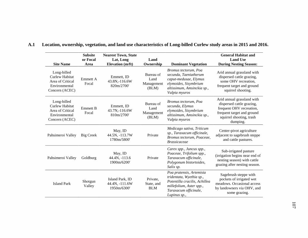
107
A.1 Location, ownership, vegetation, and land use characteristics of Long-billed Curlew study areas in 2015 and 2016.
Site Name
Subsite
or Focal
Area
Nearest Town, State
Lat, Long
Elevation (m/ft)
Land
Ownership Dominant Vegetation
General Habitat and
Land Use
During Nesting Season:
Long-billed
Curlew Habitat
Area of Critical
Environmental
Concern (ACEC)
Emmett A
Focal
Emmett, ID
43.8N,-116.6W
820m/2700'
Bureau of
Land
Management
(BLM)
Bromus tectorum, Poa
secunda, Taeniatherum
caput-medusae, Elymus
elymoides, Sisymbrium
altissimum, Amsinckia sp.,
Vulpia myuros
Arid annual grassland with
dispersed cattle grazing,
some OHV recreation,
frequent target and ground
squirrel shooting.
Long-billed
Curlew Habitat
Area of Critical
Environmental
Concern (ACEC)
Emmett B
Focal
Emmett, ID
43.7N,-116.6W
810m/2700'
Bureau of
Land
Management
(BLM)
Bromus tectorum, Poa
secunda, Elymus
elymoides, Sisymbrium
altissimum, Amsinckia sp.,
Vulpia myuros
Arid annual grassland with
dispersed cattle grazing,
frequent OHV recreation,
frequent target and ground
squirrel shooting, trash
dumping.
Pahsimeroi Valley Big Creek
May, ID
44.5N, -113.7W
1780m/5800'
Private
Medicago sativa, Triticum
sp., Taraxacum officinale,
Bromus tectorum, Poaceae,
Brassicaceae
Center-pivot agriculture
adjacent to sagebrush steppe
and cattle pastures.
Pahsimeroi Valley Goldburg
May, ID
44.4N, -113.6
1900m/6200'
Private
Carex spp., Juncus spp.,
Poaceae, Trifolium spp.,
Taraxacum officinale,
Polygonum bistortoides,
Salix sp.
Sub-irrigated pasture
(irrigation begins near end of
nesting season) with cattle
grazing after nesting season.
Island Park Shotgun
Valley
Island Park, ID
44.4N, -111.6W
1950m/6300'
Private,
State, and
BLM
Poa pratensis, Artemisia
tridentata, Wyethia sp.,
Potentilla cracilis, Achillea
millefolium, Aster spp.,
Taraxacum officinale,
Lupinus sp.,
Sagebrush steppe with
pockets of irrigated wet
meadows. Occasional access
by landowners via OHV, and
some grazing.

108
A.1 Continued.
Site Name
Subsite or
Focal Area
Nearest Town, State
Lat, Long
Elevation (m/ft)
Land
Ownership Dominant Vegetation
General Habitat and
Land Use
During Nesting Season:
Island Park Flat Ranch
Island Park, ID
44.6N, -111.3W
1960m/6400'
The Nature
Conservancy
(TNC)
Phleum pratense, Alopecurus
pratensis, Poa pratensis,
Taraxacum officincale, Potentilla
gracilis, Achillea millefolium,
Wyethia helianthoides, Trifolium
spp., Sysyrinchium montanum,
Carex spp.
Wet meadow with flood-
irrigation (after nesting
season), public access by
foot only for nature-
watching, fishing, and
some grazing after the
nesting season
Jackson
National
Elk Refuge
(NER)
Jackson, WY
43.5N, -110.7W
1940m/6400'
Federal
Bromus inermus Leyss., Stipa
comata, Agropyron cristatum (L.)
Gaertn., Alyssum alyssoides,
Taraxacum sp., Elymus
trachycaulus, Festuca idahoensis,
Poaceae, Hesperostipa comata,
Medicago sativa, Tragopogon
dubius, Phlox hoodii,
Chrysothamnus vicidoflorus
Grassland with native
ungulate grazing, weed-
control pesticide
application, pipe-fed
irrigation, jogging and
bicycling recreation on
packed gravel road.
Upper
Green
River Basin
Horse
Creek
Daniel, WY
42.9N, -110.3W
2300m/7500'
Private
Phleum pratense, Agrostis
palustris, Poa pratensis, Carex
spp., Juncus spp., Taraxacum
officinale, Potentilla sp., Trifolium
spp.
Flood-irrigated hay
pasture, bullpens, cattle
grazing
Upper
Green
River Basin
New Fork
Pinedale, WY
42.9N, -109.9W
2200m/7200'
Private
Phleum pratense, Agrostis
palustris, Poa pratensis, Carex
spp., Juncus spp., Taraxacum
officinale, Trifolium spp.
Flood-irrigated hay
pasture, bullpens, cattle
grazing

109
A.2 Initiation date summary in 2015 and 2016 for Long-billed Curlew nests.
Initiation Date
Year Site N Mean Median Range
2015
ACEC, ID 26 1-May 25-Apr 11 Apr to 27 May
Upper Green River Basin, WY 25 10-May 7-May 27 Apr to 03 Jun
Island Park, ID 13 6-May 4-May 25 Apr to 16 May
Pahsimeroi Valley, ID 17 2-May 28-Apr 20 Apr to 27 May
2016
ACEC, ID 24 1-May 29-Apr 14 Apr to 22 May
National Elk Refuge, WY 6 14-May 21-May 28 Apr to 27 May
Pahsimeroi Valley, ID 17 5-May 30-Apr 19 Apr to 01 Jun

110
A.3 Long-billed Curlew density per square km in focal nesting areas during 2015 and 2016.
Long-billed Curlews per km2 (SE)
Site Focal Nesting Area 2015 2016
ACEC, ID Emmett A Focal* 1.23 (0.32) 0.39 (0.20)
ACEC, ID Emmett B Focal* 0.91 (0.35) 0.14 (0.10)
Pahsimeroi Valley, ID Big Creek 2.74 (1.08) 2.30 (0.94)
Pahsimeroi Valley, ID Goldburg 7.29 (2.62) 6.22 (2.61)
Island Park, ID Flat Ranch 14.43 (2.26) −
Island Park, ID Shotgun Valley Focal* 2.70 (0.93) −
Jackson, WY NER − 1.27 (0.62)
Upper Green River, WY Horse Creek 9.69 (1.75) −
Upper Green River, WY New Fork 2.72 (0.74) −
*Smaller parcel within subsite delineated as a focal nesting area.

111
A.4 Qualitative assessment of mammalian predators and anthropogenic disturbance within each subsite focal area. Some
incidental sightings, especially for of mammalian predators, are presumed to be underestimates as we suspect sightings were
under-reported, and crew presence varied.
Site: Subsite
or Focal Area
Crew Size
and Effort
Mammalian Predators:
Approx. Frequency of
Incidental Sightings
Anthropogenic Disturbance:
Approx. Frequency of Incidental
Sightings
Roads/Trails: Vehicular Impact
and Access
ACEC: Emmett
A Focal
2-3 people
7 days/week
Badger: 1/day
Coyote: 1/week
Dog: 1/season
Long-tailed weasel:
2/season
Off-road travel: 2/month
On-road OHV: 1/week
Shooters: 3/week
» Public and rancher access via
several unimproved dirt roads ~2
miles from paved road and through
multiple barbed wire cattle pasture
gates
ACEC: Emmett
B Focal
Badger: 1/week
Coyote: 1/month
Off-road travel: 3/month
On-road OHV: 3/week
Shooters: 1/day
Trash dump sites: >10 in site
» Public access via paved road with
traffic flow of ~1 vehicle/min
» Many frequently-used OHV trail
networks
Pahsimeroi
Valley: Big
Creek 1 person
5 days/week
Coyote: 2/month Off-road travel: 1/season » 2-lane paved road through area with
traffic flow of ~2 vehicles/hour
Pahsimeroi
Valley:
Goldburg
Badger: 1/season
Coyote: 1/week
On-road OHV: 1/month
Off-road travel: 1/season
» 2-lane paved road through area with
traffic flow of ~2 vehicles/hour
Island Park:
Shotgun Valley
1-2 people
5 days/week
Coyote: 1/month
Fox: 1/season
On-road OHV: 1/month
Off-road travel 1/month
» 2-lane dirt road with traffic flow <1
vehicle per hour
» Several 2-track roads through site
Island Park:
Flat Ranch
Badger: 1/season
Coyote: 1/month
Dog: 1/season
Off-road travel: 1/month (workers)
On-foot ranch visitors: 2/month
» 2-lane highway to West
Yellowstone adjacent to site with
traffic flow of ~600 vehicles/hour
» Several 2-track roads through site

112
A.4 Continued.
Site: Subsite
or Focal
Area
Crew Size
and Effort
Mammalian Predators:
Approx. Frequency of
Incidental Sightings
Anthropogenic Disturbance:
Approx. Frequency of
Incidental Sightings
Roads/Trails: Vehicular Impact and
Access
Jackson:
National Elk
Refuge
(NER)
1-2 people
5 days/week
Coyote: 4/week
Wolf: 3/month
Off-road travel: 1/week (workers)
On-road bicycle: 15/day
On-road runners/walkers: 15/day
» 2-lane highway adjacent to part of site
with traffic flow of ~150 vehicles/hour
» 2-lane packed gravel road through
refuge with traffic flow of ~40
vehicles/hour
Upper Green
River Basin:
Horse Creek
2 people
5 days/week
Coyote: 6/month
Dog: 3/month
Skunk: 2/month
Ranch equipment use: 2/month » 2-lane paved highway through site
with traffic flow of ~5 vehicles/hour
» 2-lane dirt road through site with
traffic flow of <1 vehicle/hour
Upper Green
River Basin:
New Fork
Coyote: 1/month
Dog: 3/month
Skunk: 2/month
Ranch equipment use: 2/month » 1-lane paved highway adjacent to site
with traffic flow of ~290 vehicles/hour
» 1-lane gravel road through site with
traffic flow of ~5 vehicles/hour

113
APPENDIX B
Wintering Supplemental Information

114
B.1 Inter-annual Utilization Distribution Overlap Index (UDOI) for Long-billed
Curlews wintering in the Central Valley of California, the Imperial/Mexicali Valley
of California and Mexico, coastal Mexico/Baja, and inland Mexico.
Winter Season
Winter Area Winter Season ID
2014-
2015
2015-
2016
2016-
2017
Central Valley
2013-2014 AE
0.3070
2014-2015 4.3728
2015-2016 AY 5.7138
2014-2015 CC
0.3160
2015-2016 4.4159
2015-2016 EM 8.7773
Coastal
Mexico/Baja
2014-2015 AH
9.2561
2015-2016 16.0855
2014-2015 AJ
15.6933
2015-2016 3.0837
2014-2015 AN
5.8802
2015-2016 8.6424
2015-2016 ET 2.7977
2015-2016 KC 6.3420
Imperial/Mexicali
Valley
2014-2015 AA
2.6057
2015-2016 2.1751
2015-2016* CL 0.2473
2015-2016 EP 3.5397
Inland Mexico 2015-2016 CN 3.8941
2015-2016 CY 1.7738 *Cross-habitat winter compared to a single habitat winter in the 2016−2017 winter season.