Building 3D Shapes from Parts

Thesis submitted in partialfulfillment of the requirements for the

degree of Ph.D.

by

Tal Hassner

Under the Supervision of

Ronen Basri

Faculty of Mathematics and Computer Science

The Weizmann Institute of Science

Submitted to the Feinberg Graduate School of

the Weizmann Institute of Science

Rehovot 76100, Israel

December 11, 2006

Abstract

The research described in this thesis has focused on the composition of novel3D shapes (e.g., depth maps and triangulated meshes) by reusing parts ofexisting shapes. Specifically, two methods were designed [28, 27]. The firstis a novel tool for easy composition of existing 3D models (i.e., triangulatedmeshes) into novel models [28]. This tool was designed with the intention ofproviding a means for rapid modelling by 3D graphics artists. This tool wasfurther shown to have an interface which is simple enough to be automated,to a large extent, for various modelling tasks beyond composition. Thesetasks include repairing 3D models and filling-in parts of their surfaces. Thesimplicity of its interface has consequently prompted research into ways offully automating shape composition from parts. In particular, the secondoutcome of this research is a method which automatically fuses depth patchesfrom example objects, to produce a depth estimate for a novel object viewedin a single image [27]. A by-product of this reconstruction method, was thedevelopment of a system for automatic colorization of depth maps [26], whichshares much of its design with the reconstruction procedure. This thesisdescribes these three methods, and presents related, ongoing and plannedresearch.

Acknowledgements

I get by with a little help from my friendsLennon/McCartney.

The work behind this thesis required the patience, tolerance, and a greatdeal of help from both friends and family, to all of whom I am truly grateful.

First, I wish to thank Ronen Basri, for being everything a Ph.D. studentcan ever hope for in an advisor, and more. The willingness to hear outeven the most bizarre ideas, the patience to see these ideas grow, and theknowledge and wisdom to overcome problems along the way, are but a fewof the reasons why I am truly indebted to him.

I wish to thank the members of my Ph.D. committee: Shimon Ullman andMichal Irani (who was also my MS.c. advisor and always a great help). Bothhave provided an open door to any question or problem, and have offeredsound advice and help throughout my studies.

A large part of the joy I had in this work comes from the atmosphere inthe vision laboratory at Weizmann, and especially the people working there.Thank you to Eli Shechtman for putting up with my constant interrupts andquestions, and being a good friend along the way, Yaron Caspi for guidanceboth academic and otherwise, from my first days at the laboratory, YoniWexler, Bernard Sarel, Ayelet Axelrod-Balin, and Ira Kemelmacher, all ofwhich were there, ready to help with practically anything.

Long overdue thanks to Kobi Kremnizer, a close friend who basically hadto teach me math from scratch, and has been supportive from my earlieststudent days, and to Amir Ben-Amram, who’s managed to be at all times ateacher, a co-worker, and a friend.

A special heartfelt thanks goes to Lihi Zelnik-Manor, who, besides beinga great personal friend, always kept an open mind and has shown me, withcool confidence, that anything is doable.

Last, but certainly not least, I wish to thank my family. My superwomanof a wife, Osnat, who regularly managed in two minutes to make a wholeday’s worth of frustrations disappear. Thank you for putting up with me.My two amazing kids, Ben and Ella, who helped me avoid the pitfall of over-sleep and more importantly, put everything in its right perspective. Andfinally, my parents, my father Avi and mother Bruria, who have been bothexamples worth aspiring for, and an endless source of support in more waysthan I can count.

i

Table of Contents

1 Introduction 1

2 Related work 62.1 Model composition . . . . . . . . . . . . . . . . . . . . . . . . 62.2 Shape reconstruction from single images . . . . . . . . . . . . 72.3 Automatic colorization of 3D models . . . . . . . . . . . . . . 8

3 Minimal-cut model composition 103.1 System overview . . . . . . . . . . . . . . . . . . . . . . . . . 103.2 Composition framework . . . . . . . . . . . . . . . . . . . . . 12

3.2.1 Part-in-whole model placement . . . . . . . . . . . . . 123.2.2 The minimal-cut of models . . . . . . . . . . . . . . . . 123.2.3 Weighted graph representation . . . . . . . . . . . . . . 133.2.4 Mesh clipping . . . . . . . . . . . . . . . . . . . . . . . 153.2.5 Mesh stitching . . . . . . . . . . . . . . . . . . . . . . . 16

3.3 Additional applications beyond model composition . . . . . . 173.3.1 Model restoration . . . . . . . . . . . . . . . . . . . . . 173.3.2 Hole filling . . . . . . . . . . . . . . . . . . . . . . . . . 193.3.3 Model deformations . . . . . . . . . . . . . . . . . . . . 21

3.4 Implementation and results . . . . . . . . . . . . . . . . . . . 22

4 Example based 3D reconstruction from single 2D images 254.1 Estimating depth from example mappings . . . . . . . . . . . 25

4.1.1 Global optimization scheme . . . . . . . . . . . . . . . 264.1.2 Plausibility as a likelihood function . . . . . . . . . . . 284.1.3 Example update scheme . . . . . . . . . . . . . . . . . 294.1.4 Preserving global structure . . . . . . . . . . . . . . . . 32

4.2 Backside reconstruction . . . . . . . . . . . . . . . . . . . . . . 334.3 Implementation and results . . . . . . . . . . . . . . . . . . . 33

4.3.1 Representing mappings . . . . . . . . . . . . . . . . . . 334.3.2 Implementation . . . . . . . . . . . . . . . . . . . . . . 344.3.3 Experiments . . . . . . . . . . . . . . . . . . . . . . . . 34

5 Automatic Depth-Map Colorization 375.1 Image-map synthesis . . . . . . . . . . . . . . . . . . . . . . . 375.2 Accelerating synthesis . . . . . . . . . . . . . . . . . . . . . . 385.3 Implementation and results . . . . . . . . . . . . . . . . . . . 39

5.3.1 Representation of Examples . . . . . . . . . . . . . . . 395.3.2 Implementation . . . . . . . . . . . . . . . . . . . . . . 395.3.3 Experiments . . . . . . . . . . . . . . . . . . . . . . . . 39

ii

6 Conclusions and future work 426.1 A mesh based minimal-cut model composition algorithm . . . 436.2 Improving the reconstruction framework . . . . . . . . . . . . 446.3 Automatic mesh colorization . . . . . . . . . . . . . . . . . . . 45

iii

List of Figures

1 Centaur. . . . . . . . . . . . . . . . . . . . . . . . . . . . . . . 22 A typical composition session. . . . . . . . . . . . . . . . . . . 103 Part-in-whole model placement. . . . . . . . . . . . . . . . . . 134 Weighted graph construction. . . . . . . . . . . . . . . . . . . 155 Mesh clipping. . . . . . . . . . . . . . . . . . . . . . . . . . . . 166 Model restoration. . . . . . . . . . . . . . . . . . . . . . . . . 187 Automatic constraint selection. . . . . . . . . . . . . . . . . . 198 Hole filling. . . . . . . . . . . . . . . . . . . . . . . . . . . . . 209 Model deformations - arms. . . . . . . . . . . . . . . . . . . . 2110 Model deformations - head. . . . . . . . . . . . . . . . . . . . 2111 Reversing constraints. . . . . . . . . . . . . . . . . . . . . . . 2212 Minimizing user intervention. . . . . . . . . . . . . . . . . . . 2313 Multi-step composition. . . . . . . . . . . . . . . . . . . . . . 2314 Visualization of our process. . . . . . . . . . . . . . . . . . . . 2615 Summary of the basic steps of our algorithm. . . . . . . . . . . 2716 Man figure reconstruction. . . . . . . . . . . . . . . . . . . . . 2817 Graphical model representation. . . . . . . . . . . . . . . . . . 2918 Reconstruction with unknown viewing angle. . . . . . . . . . . 3119 Preserving relative position. . . . . . . . . . . . . . . . . . . . 3220 Example database mappings. . . . . . . . . . . . . . . . . . . 3321 Reconstruction failures. . . . . . . . . . . . . . . . . . . . . . . 3522 Hand reconstruction. . . . . . . . . . . . . . . . . . . . . . . . 3523 Full body reconstructions. . . . . . . . . . . . . . . . . . . . . 3624 Two face reconstructions. . . . . . . . . . . . . . . . . . . . . . 3625 Two fish reconstructions. . . . . . . . . . . . . . . . . . . . . . 3626 Image-map synthesis. . . . . . . . . . . . . . . . . . . . . . . . 3827 A detailed example of a fish image-map. . . . . . . . . . . . . 4028 Fish image-maps. . . . . . . . . . . . . . . . . . . . . . . . . . 4029 Human image-maps. . . . . . . . . . . . . . . . . . . . . . . . 4030 Bust image-maps. . . . . . . . . . . . . . . . . . . . . . . . . . 4131 Colorization failures. . . . . . . . . . . . . . . . . . . . . . . . 4132 Reconstructing a cyclops. . . . . . . . . . . . . . . . . . . . . . 4233 Combined reconstruction, pose estimation, and segmentation

result. . . . . . . . . . . . . . . . . . . . . . . . . . . . . . . . 44

iv

List of Tables

1 Transition volume dimensions and minimal cut average runtimes for various results. . . . . . . . . . . . . . . . . . . . . . 24

2 Colorization parameters for each database. . . . . . . . . . . . 41

v

1 Introduction

Computer graphics systems are becoming ubiquitous, posing a growing de-mand for both realistic and fictitious 3D models. Constructing and decorat-ing (i.e. texturing) new models from scratch is a tedious process, requiringcareful scanning of real objects and the artistic skills of trained graphicsexperts. These processes can potentially be expedited, as more and moremodels become available, by reusing parts of the geometries and textures ofexisting models. In this thesis we present the following three methods aimedat simplifying common modelling procedures by reusing information fromexample models.

1. A novel model composition tool allowing a modeler to quickly producenew models by composing parts of existing models [28].

2. A method for automatically reconstructing a plausible estimate of theshape (depth) of an object viewed in a single 2D image, by automati-cally composing parts of example objects [27].

3. A method which automatically produces structured image-maps forquery depth-maps by composing the image-maps of example objects [26].

A novel model composition tool. Consider the task of composing ex-isting models to produce a new model. With current methods this process canbe laborious, requiring a user to manually segment the input models, alignthem, and determine where to connect their parts. Automatic (e.g., [38])and semi-automatic (e.g., [23, 34, 54]) segmentation tools exist, but they arelargely inadequate for this task; segmentation tools are applied to each ofthe input models independently, and so often produce results which requirethe user to further trim the parts to eliminate undesired protrusions or tosignificantly extend the parts so that they can be connected properly. Thefirst method presented in this work is a new model composition system [28].This system, which is intended for use by both novice and expert modelers,automates much of the manual labor often associated with creating complexmodels. We further show the new operation to be particularly suitable foran assortment of model processing applications.

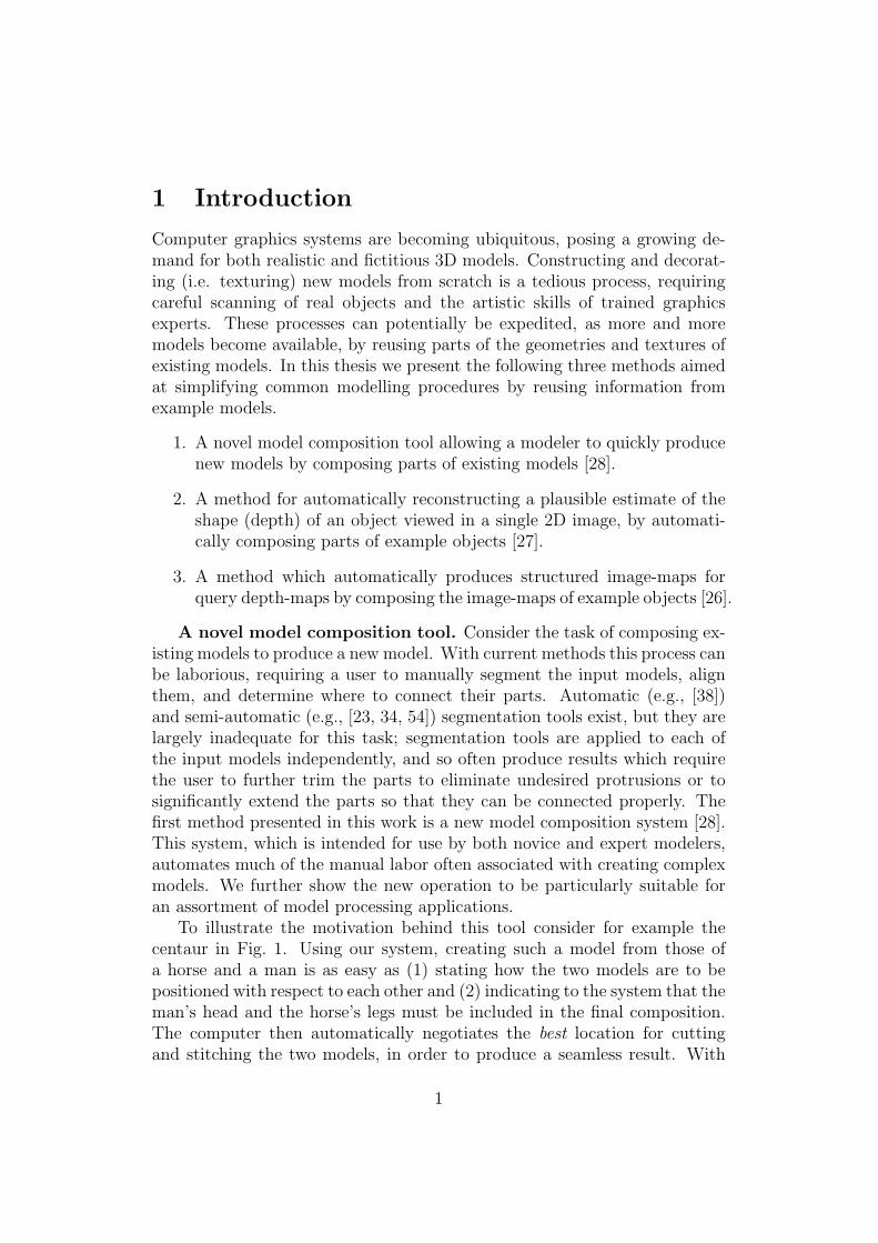
To illustrate the motivation behind this tool consider for example thecentaur in Fig. 1. Using our system, creating such a model from those ofa horse and a man is as easy as (1) stating how the two models are to bepositioned with respect to each other and (2) indicating to the system that theman’s head and the horse’s legs must be included in the final composition.The computer then automatically negotiates the best location for cuttingand stitching the two models, in order to produce a seamless result. With

1

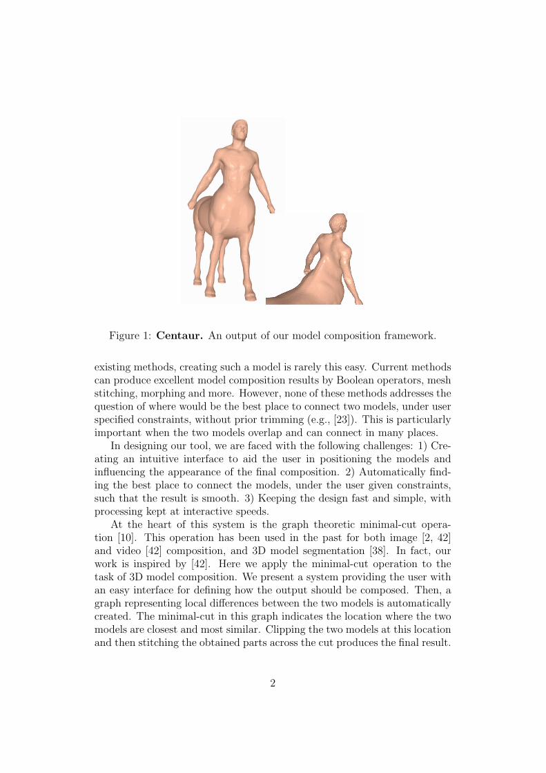
Figure 1: Centaur. An output of our model composition framework.

existing methods, creating such a model is rarely this easy. Current methodscan produce excellent model composition results by Boolean operators, meshstitching, morphing and more. However, none of these methods addresses thequestion of where would be the best place to connect two models, under userspecified constraints, without prior trimming (e.g., [23]). This is particularlyimportant when the two models overlap and can connect in many places.

In designing our tool, we are faced with the following challenges: 1) Cre-ating an intuitive interface to aid the user in positioning the models andinfluencing the appearance of the final composition. 2) Automatically find-ing the best place to connect the models, under the user given constraints,such that the result is smooth. 3) Keeping the design fast and simple, withprocessing kept at interactive speeds.

At the heart of this system is the graph theoretic minimal-cut opera-tion [10]. This operation has been used in the past for both image [2, 42]and video [42] composition, and 3D model segmentation [38]. In fact, ourwork is inspired by [42]. Here we apply the minimal-cut operation to thetask of 3D model composition. We present a system providing the user withan easy interface for defining how the output should be composed. Then, agraph representing local differences between the two models is automaticallycreated. The minimal-cut in this graph indicates the location where the twomodels are closest and most similar. Clipping the two models at this locationand then stitching the obtained parts across the cut produces the final result.

2

We note that a very similar system has recently been designed for imagesin [35].

By presenting this system, our work claims the following contributions:First, we describe a new model composition tool: Finding the best place toclip and connect overlapping models under user specified constraints. Second,we describe a novel algorithm based on graph cuts, as a means of implement-ing the new tool. Next, we detail a system designed for easy manipulationof this tool. Lastly, we show novel solutions to existing applications, basedon our proposed framework. These applications include model restoration(Fig. 6), hole filling (Fig. 8), and rigid model deformations (Fig. 9). Chap-ter 3 describes the details of this system, and demonstrates results.

Automatic reconstruction of 3D shapes from single 2D images.The development of our semi-automatic model composition tool, has nat-urally led to the question: Could this process be made fully automatic?Motivated by this question, we have designed a framework capable of esti-mating the 3D shape (depth) of an object from a single image, by piecingtogether parts of the shapes of similar looking example objects [27]. In gen-eral, the problem of estimating 3D shapes from single 2D images (i.e., ”shapereconstruction”) is ill posed, since different shapes may give rise to the sameintensity patterns. To solve this, additional constraints are required. In oursystem, we constrain the reconstruction process by assuming that similarlylooking objects from the same class (e.g., faces, fish), have similar shapes.We maintain a set of 3D objects, selected as examples of a specific class.We use these objects to produce a database of images of the objects in theclass (e.g., by standard rendering techniques), along with their respectivedepth maps. These provide examples of feasible mappings from intensitiesto shapes and are used to estimate the shapes of novel objects from singleimages.

The input to our system is an image which can often contain a novelobject. It is unlikely that the exact same image exists in our database. Wetherefore devise a method which utilizes the examples in the database toproduce novel shapes. To this end we extract portions of the image (i.e.,image patches) and seek similar intensity patterns in the example database.Matching database intensity patterns suggest possible reconstructions fordifferent portions of the image. We merge these suggested reconstructionstogether, to produce a coherent shape estimate. Thus, novel shapes areproduced by composing different parts of example objects. We show howthis scheme can be cast as an optimization process, producing the likeliestreconstruction in a graphical model representation of our problem.

A major obstacle for example based approaches is the limited size of theexample set. To faithfully represent a class, many example objects might be

3

required to account for variability in posture, texture, etc. In addition, unlessthe viewing conditions are known in advance, we may need to store for eachobject, images obtained under many conditions. This can lead to impracticalstorage and time requirements. Moreover, as the database becomes largerso does the risk of false matches, leading to degraded reconstructions. Wetherefore propose a novel example update scheme. As better estimates forthe depth are available, we generate better examples for the reconstructionon-the-fly. We are thus able to demonstrate reconstructions under unknownviews of objects from rich object classes. In addition, to reduce the num-ber of false matches we encourage the process to use example patches fromcorresponding semantic parts by adding location based constraints.

Unlike existing example based reconstruction methods, which are re-stricted to classes of highly similar shapes (e.g., faces [9]) our method pro-duces reconstructions of objects belonging to a variety of classes (e.g., hands,human figures). Similarly to existing example based methods [9, 31], ourmethod does not claim to produce accurate reconstructions, but rather plau-sible depth estimates. We show that, nonetheless, the estimates we obtainare often convincing enough.

The method we designed allows for depth reconstruction under very gen-eral conditions and requires little, if any, calibration. Our chief requirementis the existence of a 3D object database, representing the object class. Webelieve this to be a reasonable requirement given the growing availability ofsuch databases. Chapter 4 describes our method and presents depth fromsingle image results for a variety of object classes, under a variety of imagingconditions. In addition, we demonstrate how our method can be extendedto obtain plausible depth estimates of the back side of an imaged object.

Automatically coloring depth-maps. Developing our 3D reconstruc-tion scheme (Chapter 4), we observed that an almost identical frameworkcan be used to perform the task of automatic depth-map colorization [26].Coloring 3D objects by providing them with image-maps, is often an essentialstep towards producing realistic looking 3D models. The growing demandfor realistic 3D renderings has therefore prompted increasing interest in pro-ducing such detailed image-maps. Manually producing image-maps for 3Dobjects can be a tedious task, made harder when rendering masses of models(e.g., crowds), where separate image-maps must be crafted for each individ-ual object. Although automatic colorization methods exist, they have mostlyfocused on texture synthesis on 3D surfaces. Specifically, these methods uni-formly cover models with input texture samples. Thus, they do not solve theproblem of producing realistic image-maps for non-textural objects, whichmake up much of the world around us. Take for example objects such aspeople. Although covering a 3D model of a human, from head to toe with

4

texture (e.g., grass, hair), might look interesting, it will by no means berealistic.

To speed up the modeling pipeline and improve the quality of availableimage-maps, we demonstrate how our system can be used for automaticsynthesis of custom image-maps for novel shapes. We observe that if objectshave similar structures, they can often share similar appearances. Our systemthus uses a database of example objects and their image-maps, all from thesame class (e.g., fish, busts), to synthesize appearances for novel objects ofthe same class. Given a novel object, we borrow parts of example maps, andseamlessly merge them, producing an image-map tailored to each object’s 3Dstructure. When a single database object is used, this effectively performsan automatic morph of the database image-map to fit the 3D features of theinput depth.

Our desired output is an image-map which both fits the 3D features ofthe input object, and appears similar to maps in our database. Similarly toour reconstruction framework, we claim that this goal can be expressed asa global target function, and optimized via a hard-EM process. Chapter 5describes the modifications applied to the reconstruction framework, to allowfor image-map synthesis. It concludes with a short discussion of currentattempts to extend this idea to colorize meshes, not depth-maps.

5

2 Related work

We next review existing work, pertaining to the three systems developedas part of this research. We note that some of the mentioned papers werepublished after our own work.

2.1 Model composition

Recently, several model composition frameworks have been proposed, focus-ing on simplifying the process of positioning, cutting, and composing existingmodels (e.g., [23, 34, 54]). In these systems, new models are created by cut-ting each input model separately, using semi-automatic segmentation tools(e.g., “Intelligent scissors” [23], “Easy mesh cutting” [34]), then stitchingthem to form the composition result. As models are cut independently ofeach other, large gaps often separate their borders. These gaps must then beinterpolated by the stitching algorithm. Our model composition system, onthe other hand, clips models against each other, leaving only the smallest ofgaps between their borders, allowing them to be connected with little or novisible artifacts. In addition, our interface does not rely on prior segmenta-tion of the models and is simple enough to allow for automation, to a largeextent, for certain applications (see Chapter 3.3).

In Constructive Solid Geometry (CSG) model primitives are combinedusing Boolean operations including union, intersection and subtraction (seeoverview in [30]). Such operations were adapted for numerous model repre-sentations [1, 7, 44, 47]. Although very intuitive, our proposed model compo-sition tool cannot generally be specified as a sequence of Boolean operations.Specifically, reproducing our results using Boolean operations requires pre-processing of the input models in order to remove all undesired parts (see forexample the centaur result of [1] where the horse’s head and the man’s waistwere removed before union.)

The problem of mesh stitching has enjoyed much attention, ranging fromthe Zippering system of [58], to more recent methods such as [8, 37, 67].These produce seamless model compositions even if the input models havesignificantly different borders, separated by large gaps. These methods, how-ever, assume that there is no ambiguity about where the two models shouldconnect (e.g., [37, 67]), or alternatively blend the two models in all locationswhere they connect(e.g., [58]). Our method, on the other hand, handlespractical cases where two overlapping models can connect smoothly in manyplaces. Given user constraints, it selects a single location through which thetwo models should connect, cutting and stitching them when necessary.

In addition to model composition, we propose our tool as a new solution

6

to problems such as hole filling, restoration, and piecewise rigid deformations.Existing methods solve these problems in a variety of ways. Hole filling andrestoration are often performed using diffusion based methods (e.g., [16, 60]).Diffusion, however, can only complete smooth surfaces. For example, if anose were missing from a face, a diffusion based approach would fill the holesmoothly, generating a nose-less face. Two recent methods, [4] and [53], wereshown to produce excellent results even for non-smooth models. The formermorphs an ideal model prototype onto the flawed model. The latter coversflaws in the input model with surface patches taken from un-flawed parts ofthe same model. Our method shares some ideas with [53], however, all themethods mentioned above are specific to hole filling, and it is unclear how toextend them to other applications, such as general model composition.

There are multitudes of existing methods for deforming models. Theseinclude morphing (e.g., [3]), skeleton based methods (see survey in [12]),example based methods (e.g., [55]), and more. We do not presume to replacethese sophisticated methods, however, we have found that often our tooloffers a simple, “quick and dirty” alternative for applying piecewise rigiddeformations to models. The simplicity of our tool can be highly beneficialto unskilled users as it can easily deform models using a trivial interface (e.g.,it does not require assigning skin elasticity properties etc.).

Finally, the graph-theoretic minimal cut operation has been used in thepast for model cutting and segmentation (e.g., [38, 54]). The method pro-posed in this research is the first to use cuts for model composition. In awork published after our own, minimal-cut was used for model composition,as a means of implementing a system for textural model generation [69]. Wenote that their implementation is different than our own. In particular, un-like our own implementation, their minimal-cut operation does not guaranteethat the cut would produce matching borders between the two models to becomposed, and so require additional local morphing of the two model beforestitching.

2.2 Shape reconstruction from single images

Methods for single image reconstruction commonly use cues such as shad-ing, silhouette shapes, texture, and vanishing points [13, 15, 24, 33, 65].These methods restrict the allowable reconstructions by placing constraintson the properties of reconstructed objects (e.g., reflectance properties, view-ing conditions, and symmetry). A few approaches explicitly use examples toguide the reconstruction process. One approach [31, 32] reconstructs outdoorscenes assuming they can be labelled as “ground,” “sky,” and “vertical” bill-boards. A second notable approach makes the assumption that all 3D objects

7

in the class being modelled lie in a linear space spanned using a few basisobjects (e.g., [6, 9, 17, 51]). This approach is applicable to faces, but it isless clear how to extend it to more variable classes because it requires densecorrespondences between surface points across examples. Here, we assumethat the object viewed in the query image has similar looking counterparts inour example set. Semi-automatic tools are another approach to single imagereconstruction [45, 68]. Our method, however, is automatic, requiring onlya fixed number of numeric parameters.

We produce depth for a query image in a manner reminiscent of example-based texture synthesis methods [20, 61]. Subsequent publications have sug-gested additional applications for these synthesis schemes [18, 19, 29]. Wenote in particular, the connection between our method, and Image Analo-gies [29]. Using their jargon, taking the pair A and A’ to be the databaseimage and depth, and B to be the query image, B’, the synthesized result,would be the query’s depth estimate. Their method, however, cannot beused to recover depth under an unknown viewing position, nor handle largedata sets. The optimization method we use here is motivated by the methodintroduced by [64] for image and video hole-filling, and [41] for texture syn-thesis. In [41] this optimization method was shown to be comparable to thestate of the art in texture synthesis.

2.3 Automatic colorization of 3D models

Automatic methods for decorating 3D models have mostly focused on cover-ing the surface of 3D models with texture examples (e.g., [57, 62, 66]). Wenote in particular a work concurrent to our own [25], which uses the sameoptimization used in our work (for both 3D reconstruction and depth mapcolorization). Their application, however, is covering 3D surfaces with a 2Dtexture example.

Recent methods have attempted to allow the modeler semi-automaticmeans of producing non-textural image-maps (e.g., [70]). Their work relayson the user forming explicit correspondences between parts of the 3D surface,and different texture examples, which are then merged together to producethe complete image-map for an input 3D model. Our work, on the otherhand, is fully automatic.

Finally, there have been a number of publications presenting methods formodel correspondences and Cross-Parameterization (e.g., [40, 48]) . Thesemethods establish correspondences across two or more models. Once thesecorrespondences are computed, surface properties such as texture, can betransferred from one corresponding model to another, providing the newmodel with a custom image-map. These methods, however, often require the

8

modeler to input a seed set of correspondences across the models, or elseassume the models are similar in general form. In our colorization method,no prior correspondences are required, the process is fully automatic, and themodels need only be locally similar.

9

3 Minimal-cut model composition

The following chapter describes our semi-automatic model composition frame-work, following [28].

3.1 System overview

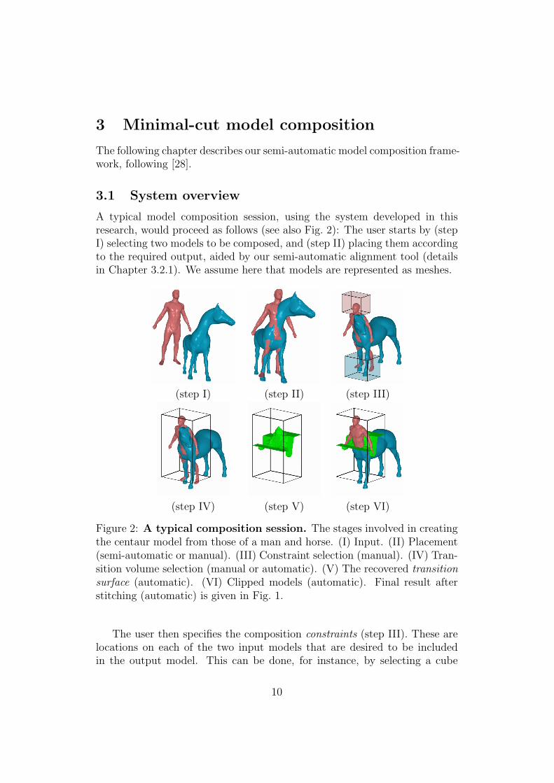
A typical model composition session, using the system developed in thisresearch, would proceed as follows (see also Fig. 2): The user starts by (stepI) selecting two models to be composed, and (step II) placing them accordingto the required output, aided by our semi-automatic alignment tool (detailsin Chapter 3.2.1). We assume here that models are represented as meshes.

(step I) (step II) (step III)

(step IV) (step V) (step VI)

Figure 2: A typical composition session. The stages involved in creatingthe centaur model from those of a man and horse. (I) Input. (II) Placement(semi-automatic or manual). (III) Constraint selection (manual). (IV) Tran-sition volume selection (manual or automatic). (V) The recovered transitionsurface (automatic). (VI) Clipped models (automatic). Final result afterstitching (automatic) is given in Fig. 1.

The user then specifies the composition constraints (step III). These arelocations on each of the two input models that are desired to be includedin the output model. This can be done, for instance, by selecting a cube

10

in space that contains the constraint region, selecting a segment from a seg-mentation output, or even marking a single point. The constraints for eachinput model are thus a subset of its surface and as such are independent ofthe global position of the model. To constrain our algorithm to produce thecentaur in Fig. 1, for example, we selected the man’s head and the horse’slegs (Fig. 2, step III). The rest of the centaur was extracted automaticallyby the algorithm.

A transition volume can also be specified (step IV). This is an additionalmeans of controlling the final output, by confining where the models areallowed to connect. By default models can connect anywhere, which is to saythe default transition volume is the bounding box of the models’ union. Theuser may specify a different transition volume by drawing an appropriatebox. The models would then be allowed to connect only within this userdefined volume.

The system then proceeds to automatically cut and stitch the models.First, a weighted graph is constructed, (details in Chapters 3.2.2 and 3.2.3)reflecting local differences between the two models in the transition volume.This graph is then cut using a minimal cut method. The graph cut representsa surface separating the transition volume into disjoint sub-volumes (stepV). We call this the transition surface, as it determines where the modelsshould be cut and stitched, or rather, where the transition from one modelto the other occurs. The weights associated with each edge in the graphensure that this surface passes where the models are closest and most similar,which in return ensures that the resulting composition will be smooth. Bothmodels are then clipped (Chapter 3.2.4) at the transition surface (step VI)and stitched (Chapter 3.2.5) across it to produce the final result (Fig. 1).

The user is now free to accept the composition or make further changes toeither position, constraints or transition volume. Note that in making subse-quent changes to any of the positions, there is no need to reselect constraints.The constraints, being parts of input models’ surfaces, are unaffected by theparticular position of each model. This allows quick review of different modelarrangements.

Our interface is trivial, requiring only a few intuitive boxes to be roughlydrawn around parts of the models. As a consequence, this tool can easily beautomated, opening up the possibility of using it for a variety of applications(a few are suggested in Chapter 3.3). We next offer a detailed look at thedifferent stages in our system.

11

3.2 Composition framework

3.2.1 Part-in-whole model placement

We provide the modeler with a graphical interface capable of applying rigidtransformations (i.e., translation, rotation, scale and mirror) to each model,allowing anyone with passing knowledge of modeling software to arrangethem as required in a few short minutes. In addition, having designed oursystem for both expert and novice users, we provide a tool for semi automaticmodel alignment.

Most work on alignment is based on searching for an optimal alignmentof complete models [52]. However, for our purposes we found this often to beinappropriate. For example, aligning the man and horse from Fig. 2 will placethe man horizontally along the horse’s back. Our goal is therefore different.We wish to find an optimal “part-in-whole” alignment. In other words, werequire an optimal alignment of “emphasized” parts (e.g., the heads of thecow and dog in Fig. 3), and not of whole models. Models thus aligned,share overlapping surfaces in the selected parts, which can then be smoothlyconnected (Fig. 3).

Unlike alignment methods proposed in computer vision which use mostlyfeature points and lines, we use segmentation [38] as an aid. This segmen-tation can be semi-manual or automatic. All the user needs to do is selectthe emphasized parts and the system then aligns the whole models automat-ically. For the actual part-to-part alignment algorithm, we use PCA [36] toobtain a coarse guess for the rigid transformation between the selected parts.Standard ICP [52] is then used to refine the guess and recover the final partto part alignment.

3.2.2 The minimal-cut of models

Once the user arranges models A and B (either manually or by using an align-ment tool) and selects the constraints, the system proceeds automatically tocut and stitch them. This is achieved by running an optimization procedureto find the best location for a transition from one model to another, on eachof the two models (within the transition volume). To implement this opti-mization procedure we construct a weighted graph G = (V, E) with nodes inV representing locations, edges in E encoding neighborhoods, and weightsassociated with the edges, expressing the (inverse) likelihood of transitions(i.e., low cost implies smooth transition from one model to another). Auxil-iary source and target nodes are added to this graph and are connected tothe constrained regions in each model. The best transition is then found bycomputing the minimal cut in the graph (using a max flow algorithm). A

12

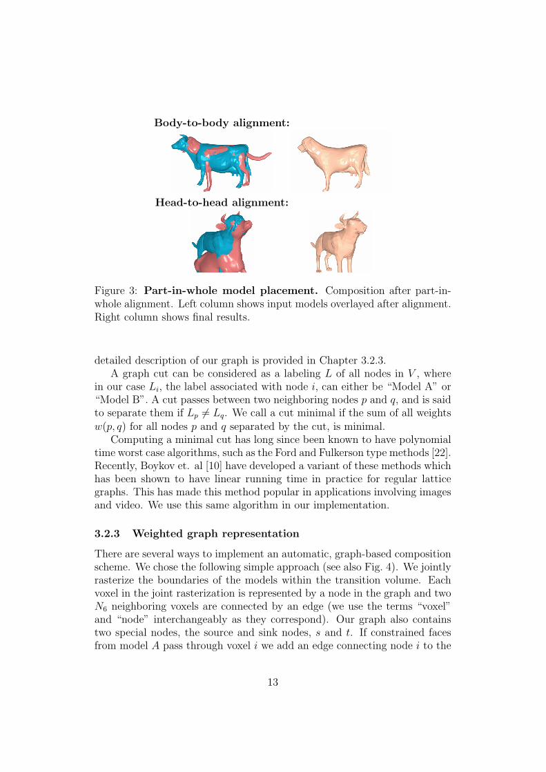
Body-to-body alignment:

Head-to-head alignment:

Figure 3: Part-in-whole model placement. Composition after part-in-whole alignment. Left column shows input models overlayed after alignment.Right column shows final results.

detailed description of our graph is provided in Chapter 3.2.3.A graph cut can be considered as a labeling L of all nodes in V , where

in our case Li, the label associated with node i, can either be “Model A” or“Model B”. A cut passes between two neighboring nodes p and q, and is saidto separate them if Lp 6= Lq. We call a cut minimal if the sum of all weightsw(p, q) for all nodes p and q separated by the cut, is minimal.

Computing a minimal cut has long since been known to have polynomialtime worst case algorithms, such as the Ford and Fulkerson type methods [22].Recently, Boykov et. al [10] have developed a variant of these methods whichhas been shown to have linear running time in practice for regular latticegraphs. This has made this method popular in applications involving imagesand video. We use this same algorithm in our implementation.

3.2.3 Weighted graph representation

There are several ways to implement an automatic, graph-based compositionscheme. We chose the following simple approach (see also Fig. 4). We jointlyrasterize the boundaries of the models within the transition volume. Eachvoxel in the joint rasterization is represented by a node in the graph and twoN6 neighboring voxels are connected by an edge (we use the terms “voxel”and “node” interchangeably as they correspond). Our graph also containstwo special nodes, the source and sink nodes, s and t. If constrained facesfrom model A pass through voxel i we add an edge connecting node i to the

13

source s (Fig. 4.b). Similarly, if constrained faces in B pass through a voxel,we connect it to the sink t.

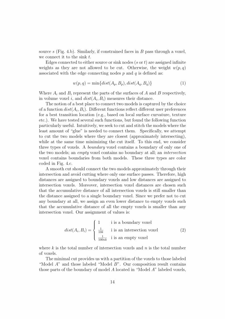
Edges connected to either source or sink nodes (s or t) are assigned infiniteweights as they are not allowed to be cut. Otherwise, the weight w(p, q)associated with the edge connecting nodes p and q is defined as:

w(p, q) = min{dist(Ap, Bp), dist(Aq, Bq)} (1)

Where Ai and Bi represent the parts of the surfaces of A and B respectively,in volume voxel i, and dist(Ai, Bi) measures their distance.

The notion of a best place to connect two models is captured by the choiceof a function dist(Ai, Bi). Different functions reflect different user preferencesfor a best transition location (e.g., based on local surface curvature, textureetc.). We have tested several such functions, but found the following functionparticularly useful. Intuitively, we seek to cut and stitch the models where theleast amount of “glue” is needed to connect them. Specifically, we attemptto cut the two models where they are closest (approximately intersecting),while at the same time minimizing the cut itself. To this end, we considerthree types of voxels. A boundary voxel contains a boundary of only one ofthe two models; an empty voxel contains no boundary at all; an intersectionvoxel contains boundaries from both models. These three types are colorcoded in Fig. 4.c.

A smooth cut should connect the two models approximately through theirintersection and avoid cutting where only one surface passes. Therefore, highdistances are assigned to boundary voxels and low distances are assigned tointersection voxels. Moreover, intersection voxel distances are chosen suchthat the accumulative distance of all intersection voxels is still smaller thanthe distance assigned to a single boundary voxel. Since we prefer not to cutany boundary at all, we assign an even lower distance to empty voxels suchthat the accumulative distance of all the empty voxels is smaller than anyintersection voxel. Our assignment of values is:

dist(Ai, Bi) =

1 i is a boundary voxel

110k

i is an intersection voxel

1100nk

i is an empty voxel

(2)

where k is the total number of intersection voxels and n is the total numberof voxels.

The minimal cut provides us with a partition of the voxels to those labeled“Model A” and those labeled “Model B”. Our composition result containsthose parts of the boundary of model A located in “Model A” labeled voxels,

14

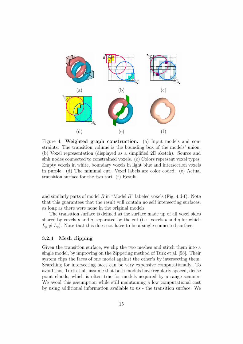
(a) (b) (c)

(d) (e) (f)

Figure 4: Weighted graph construction. (a) Input models and con-straints. The transition volume is the bounding box of the models’ union.(b) Voxel representation (displayed as a simplified 2D sketch). Source andsink nodes connected to constrained voxels. (c) Colors represent voxel types.Empty voxels in white, boundary voxels in light blue and intersection voxelsin purple. (d) The minimal cut. Voxel labels are color coded. (e) Actualtransition surface for the two tori. (f) Result.

and similarly parts of model B in “Model B” labeled voxels (Fig. 4.d-f). Notethat this guarantees that the result will contain no self intersecting surfaces,as long as there were none in the original models.

The transition surface is defined as the surface made up of all voxel sidesshared by voxels p and q, separated by the cut (i.e., voxels p and q for whichLp 6= Lq). Note that this does not have to be a single connected surface.

3.2.4 Mesh clipping

Given the transition surface, we clip the two meshes and stitch them into asingle model, by improving on the Zippering method of Turk et al. [58]. Theirsystem clips the faces of one model against the other’s by intersecting them.Searching for intersecting faces can be very expensive computationally. Toavoid this, Turk et al. assume that both models have regularly spaced, densepoint clouds, which is often true for models acquired by a range scanner.We avoid this assumption while still maintaining a low computational costby using additional information available to us - the transition surface. We

15

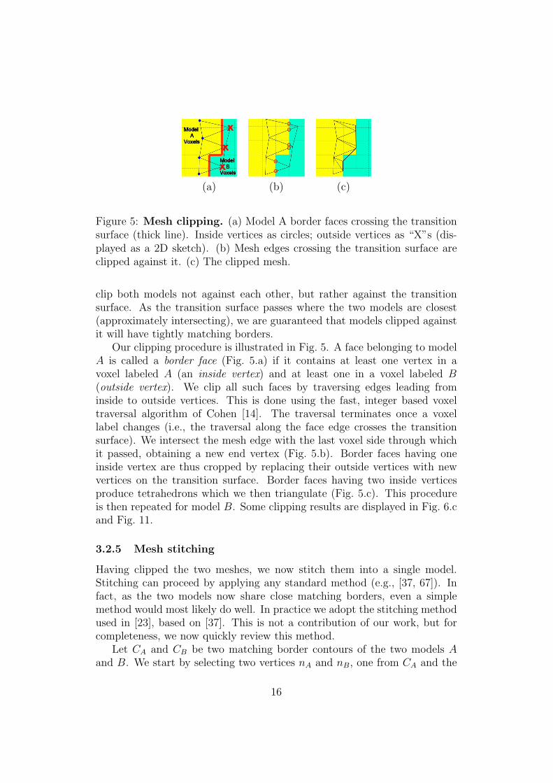
(a) (b) (c)

Figure 5: Mesh clipping. (a) Model A border faces crossing the transitionsurface (thick line). Inside vertices as circles; outside vertices as “X”s (dis-played as a 2D sketch). (b) Mesh edges crossing the transition surface areclipped against it. (c) The clipped mesh.

clip both models not against each other, but rather against the transitionsurface. As the transition surface passes where the two models are closest(approximately intersecting), we are guaranteed that models clipped againstit will have tightly matching borders.

Our clipping procedure is illustrated in Fig. 5. A face belonging to modelA is called a border face (Fig. 5.a) if it contains at least one vertex in avoxel labeled A (an inside vertex) and at least one in a voxel labeled B(outside vertex). We clip all such faces by traversing edges leading frominside to outside vertices. This is done using the fast, integer based voxeltraversal algorithm of Cohen [14]. The traversal terminates once a voxellabel changes (i.e., the traversal along the face edge crosses the transitionsurface). We intersect the mesh edge with the last voxel side through whichit passed, obtaining a new end vertex (Fig. 5.b). Border faces having oneinside vertex are thus cropped by replacing their outside vertices with newvertices on the transition surface. Border faces having two inside verticesproduce tetrahedrons which we then triangulate (Fig. 5.c). This procedureis then repeated for model B. Some clipping results are displayed in Fig. 6.cand Fig. 11.

3.2.5 Mesh stitching

Having clipped the two meshes, we now stitch them into a single model.Stitching can proceed by applying any standard method (e.g., [37, 67]). Infact, as the two models now share close matching borders, even a simplemethod would most likely do well. In practice we adopt the stitching methodused in [23], based on [37]. This is not a contribution of our work, but forcompleteness, we now quickly review this method.

Let CA and CB be two matching border contours of the two models Aand B. We start by selecting two vertices nA and nB, one from CA and the

16

other from CB, which are the closest of all such pairs. Let n′A be the vertex10% of the way around CA starting at nA, and n′B be similarly defined onCB. The dot product of the two vectors, the one from nA to n′A and theother from nB to n′B, gives us the orientation around CA and CB. Vertexcorrespondences are then set between CA and CB iteratively. Starting at nA

and nB and proceeding along the curve for which the next vertex is closest, wematch vertices by adding edges between them, creating new faces. Havingthus sealed the gap between the two models, we allow the user to furthersmooth the new boundary by averaging vertex positions by their neighbors auser specified number of iterations, applied to vertices at a distance no largerthan a user specified threshold, using user defined weights.

Figures 11, 12 and 13 illustrate various charasteristics of the suggestedcomposition framework.

3.3 Additional applications beyond model composition

The system we described thus far has a trivial interface. It can therefore beeasily automated, to a large extent, and applied as a unified solution to avariety of model processing tasks. We next describe a few such examples.

3.3.1 Model restoration

We allow a modeler easy means of repairing flawed models (e.g., scarred mod-els) by replacing defective boundary patches with perfect surfaces obtainedfrom a model database. The user selects the flawed boundary (the query) bydrawing a box around it (Fig. 6.a). Our system then searches a database ofmodels for a surface most similar to the one selected by the user (we describeour search method below). Once found, the recovered surface patch is thenautomatically cut and pasted into the original model using the minimal cuttool. Our results in Fig. 6 can be compared to those of [53] and [44] obtainedon the same bust model.

To automate the process, we take the user drawn box around the flaw asthe transition volume. Constraints are selected by the system as follows: Weassume that the flaw in the input model is roughly at the center of the userdrawn box (i.e., the center of the query). Constraints on the flawed model aretherefore selected to be faces furthest from the flaw, i.e., faces closest to thesides of the transition volume. Constraints on the database model chosento repair the flaw are selected closest to the flaw, in other words, closestto the center of the transition volume. Both constraints are illustrated inFig. 7.a. The actual distances from the center of the volume, and its sidesare governed by a user defined parameter. We found the results to be robust

17

to these values.

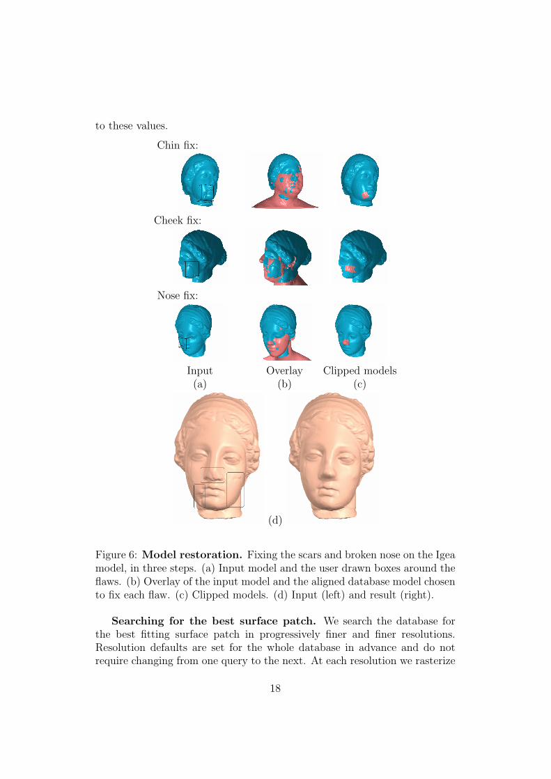
Chin fix:

Cheek fix:

Nose fix:

Input Overlay Clipped models(a) (b) (c)

(d)

Figure 6: Model restoration. Fixing the scars and broken nose on the Igeamodel, in three steps. (a) Input model and the user drawn boxes around theflaws. (b) Overlay of the input model and the aligned database model chosento fix each flaw. (c) Clipped models. (d) Input (left) and result (right).

Searching for the best surface patch. We search the database forthe best fitting surface patch in progressively finer and finer resolutions.Resolution defaults are set for the whole database in advance and do notrequire changing from one query to the next. At each resolution we rasterize

18

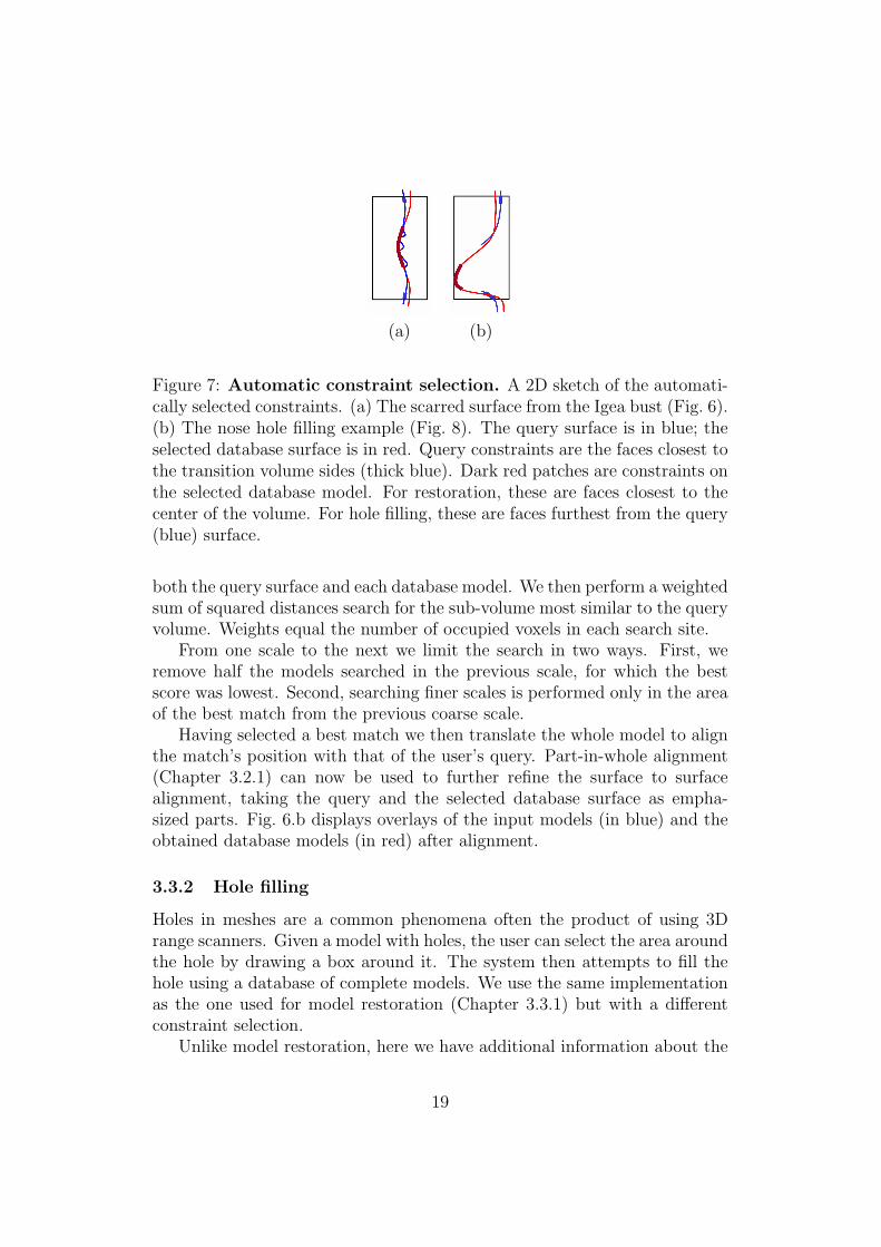
(a) (b)

Figure 7: Automatic constraint selection. A 2D sketch of the automati-cally selected constraints. (a) The scarred surface from the Igea bust (Fig. 6).(b) The nose hole filling example (Fig. 8). The query surface is in blue; theselected database surface is in red. Query constraints are the faces closest tothe transition volume sides (thick blue). Dark red patches are constraints onthe selected database model. For restoration, these are faces closest to thecenter of the volume. For hole filling, these are faces furthest from the query(blue) surface.

both the query surface and each database model. We then perform a weightedsum of squared distances search for the sub-volume most similar to the queryvolume. Weights equal the number of occupied voxels in each search site.

From one scale to the next we limit the search in two ways. First, weremove half the models searched in the previous scale, for which the bestscore was lowest. Second, searching finer scales is performed only in the areaof the best match from the previous coarse scale.

Having selected a best match we then translate the whole model to alignthe match’s position with that of the user’s query. Part-in-whole alignment(Chapter 3.2.1) can now be used to further refine the surface to surfacealignment, taking the query and the selected database surface as empha-sized parts. Fig. 6.b displays overlays of the input models (in blue) and theobtained database models (in red) after alignment.

3.3.2 Hole filling

Holes in meshes are a common phenomena often the product of using 3Drange scanners. Given a model with holes, the user can select the area aroundthe hole by drawing a box around it. The system then attempts to fill thehole using a database of complete models. We use the same implementationas the one used for model restoration (Chapter 3.3.1) but with a differentconstraint selection.

Unlike model restoration, here we have additional information about the

19

Nose Completion:

Head Completion:

Input Result

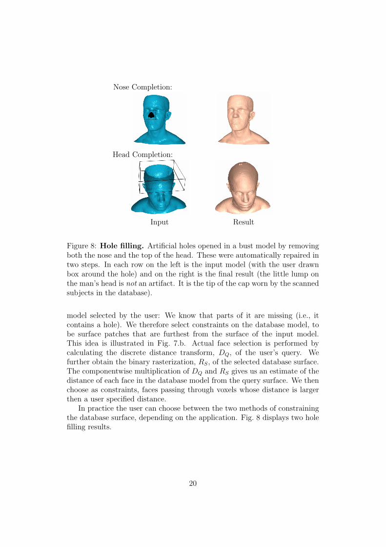
Figure 8: Hole filling. Artificial holes opened in a bust model by removingboth the nose and the top of the head. These were automatically repaired intwo steps. In each row on the left is the input model (with the user drawnbox around the hole) and on the right is the final result (the little lump onthe man’s head is not an artifact. It is the tip of the cap worn by the scannedsubjects in the database).

model selected by the user: We know that parts of it are missing (i.e., itcontains a hole). We therefore select constraints on the database model, tobe surface patches that are furthest from the surface of the input model.This idea is illustrated in Fig. 7.b. Actual face selection is performed bycalculating the discrete distance transform, DQ, of the user’s query. Wefurther obtain the binary rasterization, RS, of the selected database surface.The componentwise multiplication of DQ and RS gives us an estimate of thedistance of each face in the database model from the query surface. We thenchoose as constraints, faces passing through voxels whose distance is largerthen a user specified distance.

In practice the user can choose between the two methods of constrainingthe database surface, depending on the application. Fig. 8 displays two holefilling results.

20

3.3.3 Model deformations

In this Chapter we suggest our tool as a simple, “quick and dirty” method forapplying piecewise rigid deformations to models and for generating simple 3Danimations. Our idea is to take a straightforward approach to deformation.That is, we clone the model and allow the user to change the clone’s positionwith respect to the original model (i.e., apply rotation, translation etc.) Oursystem then automatically cuts and stitches the two models, producing thedesired deformation.

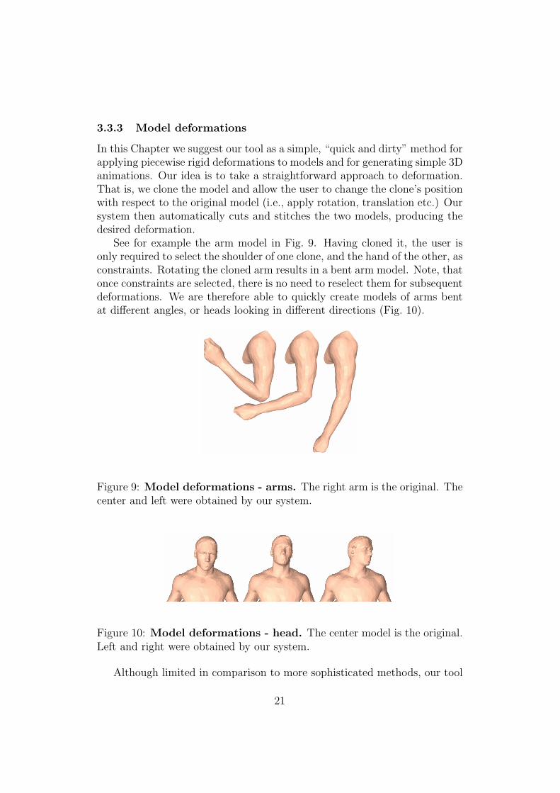
See for example the arm model in Fig. 9. Having cloned it, the user isonly required to select the shoulder of one clone, and the hand of the other, asconstraints. Rotating the cloned arm results in a bent arm model. Note, thatonce constraints are selected, there is no need to reselect them for subsequentdeformations. We are therefore able to quickly create models of arms bentat different angles, or heads looking in different directions (Fig. 10).

Figure 9: Model deformations - arms. The right arm is the original. Thecenter and left were obtained by our system.

Figure 10: Model deformations - head. The center model is the original.Left and right were obtained by our system.

Although limited in comparison to more sophisticated methods, our tool

21

does allow even unskilled users to easily deform models. Compare, for ex-ample, our arm results (Fig. 9) to those obtained by interpolating modelsin [55].

3.4 Implementation and results

Our system is currently implemented in C++ and MATLAB. The minimalcut is obtained using the code made available by Boykov et. al [10]. The userinterface for model arrangement, constraints and transition volume selectionis 3D Studio Max.

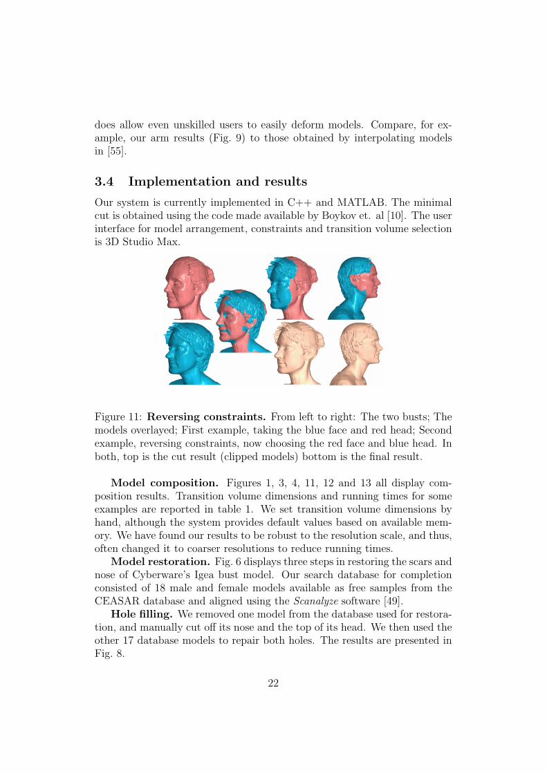
Figure 11: Reversing constraints. From left to right: The two busts; Themodels overlayed; First example, taking the blue face and red head; Secondexample, reversing constraints, now choosing the red face and blue head. Inboth, top is the cut result (clipped models) bottom is the final result.

Model composition. Figures 1, 3, 4, 11, 12 and 13 all display com-position results. Transition volume dimensions and running times for someexamples are reported in table 1. We set transition volume dimensions byhand, although the system provides default values based on available mem-ory. We have found our results to be robust to the resolution scale, and thus,often changed it to coarser resolutions to reduce running times.

Model restoration. Fig. 6 displays three steps in restoring the scars andnose of Cyberware’s Igea bust model. Our search database for completionconsisted of 18 male and female models available as free samples from theCEASAR database and aligned using the Scanalyze software [49].

Hole filling. We removed one model from the database used for restora-tion, and manually cut off its nose and the top of its head. We then used theother 17 database models to repair both holes. The results are presented inFig. 8.

22

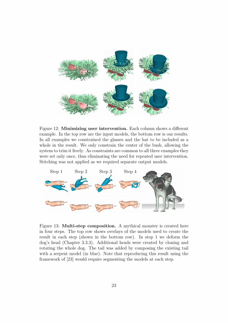
Figure 12: Minimizing user intervention. Each column shows a differentexample. In the top row are the input models, the bottom row is our results.In all examples we constrained the glasses and the hat to be included as awhole in the result. We only constrain the center of the bush, allowing thesystem to trim it freely. As constraints are common to all three examples theywere set only once, thus eliminating the need for repeated user intervention.Stitching was not applied as we required separate output models.

Step 1 Step 2 Step 3 Step 4

Figure 13: Multi-step composition. A mythical monster is created herein four steps. The top row shows overlays of the models used to create theresult in each step (shown in the bottom row). In step 1 we deform thedog’s head (Chapter 3.3.3). Additional heads were created by cloning androtating the whole dog. The tail was added by composing the existing tailwith a serpent model (in blue). Note that reproducing this result using theframework of [23] would require segmenting the models at each step.

23

Example Dim. Time

Centaur (Fig. 1) 34×56×26 1 secDog-cow (Fig. 3) 84×61×37 4 secShades (Fig. 12) 155×71×142 16 secTop hat (Fig. 12) 104×76×92 40 secCerberus (Fig. 13) 29×32×29 0.3 sec

Table 1: Transition volume dimensions and minimal cut averagerun times for various results. All run times were obtained on a standard2.6MHz processor PC running WinXP.

24

4 Example based 3D reconstruction from sin-

gle 2D images

In this chapter, we describe our 3D reconstruction framework, as originallypresented in [27].

4.1 Estimating depth from example mappings

Given a query image I of some object of a certain class, our goal is to esti-mate a depth map D for the object. To determine depth our process usesexamples of feasible mappings from intensities to depths for the class. Thesemappings are given in a database S = {Mi}n

i=1 = {(Ii, Di)}ni=1, where Ii and

Di respectively are the image and the depth map of an object from the class.For simplicity we assume first that all the images in the database containobjects viewed in the same viewing position as in the query image. We relaxthis requirement later in Sec. 4.1.3.

Our process attempts to associate a depth map D to the query imageI, such that every patch of mappings in M = (I, D) will have a matchingcounterpart in S. We call such a depth map a plausible depth estimate. Ourbasic approach to obtaining such a depth is as follows (see also Fig. 14). Atevery location p in I we consider a k × k window around p. For each suchwindow, we seek a matching window in the database with a similar intensitypattern in the least squares sense (Fig. 14.(i)). Once such a window is foundwe extract its corresponding k × k depths. We do this for all pixels inI, matching overlapping intensity patterns and obtaining k2 best matchingdepth estimates for every pixel. The depth value at every p is then determinedby taking an average of these k2 estimates (Fig. 14.(ii)).

There are several reasons why this approach, on its own, is insufficientfor reconstruction.

• The depth at each pixel is selected independently of its neighbors. Thisdoes not guarantee that patches in M will be consistent with thosein the database. To obtain a depth which is consistent with bothinput image and depth examples we therefore require a strong globaloptimization procedure. We describe such a procedure in Sec. 4.1.1.

• Capturing the variability of posture and viewing angles of even a simpleclass of objects, with a fixed set of example mappings may be very diffi-cult. We thus propose an online database update scheme in Sec. 4.1.3.

• Similar intensity patterns may originate from different semantic parts,with different depths, resulting in poor reconstructions. We propose

25

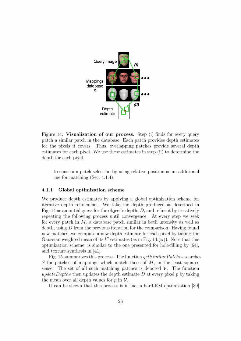
Figure 14: Visualization of our process. Step (i) finds for every querypatch a similar patch in the database. Each patch provides depth estimatesfor the pixels it covers. Thus, overlapping patches provide several depthestimates for each pixel. We use these estimates in step (ii) to determine thedepth for each pixel.

to constrain patch selection by using relative position as an additionalcue for matching (Sec. 4.1.4).

4.1.1 Global optimization scheme

We produce depth estimates by applying a global optimization scheme foriterative depth refinement. We take the depth produced as described inFig. 14 as an initial guess for the object’s depth, D, and refine it by iterativelyrepeating the following process until convergence. At every step we seekfor every patch in M , a database patch similar in both intensity as well asdepth, using D from the previous iteration for the comparison. Having foundnew matches, we compute a new depth estimate for each pixel by taking theGaussian weighted mean of its k2 estimates (as in Fig. 14.(ii)). Note that thisoptimization scheme, is similar to the one presented for hole-filling by [64],and texture synthesis in [41].

Fig. 15 summarizes this process. The function getSimilarPatches searchesS for patches of mappings which match those of M , in the least squaressense. The set of all such matching patches is denoted V . The functionupdateDepths then updates the depth estimate D at every pixel p by takingthe mean over all depth values for p in V .

It can be shown that this process is in fact a hard-EM optimization [39]

26

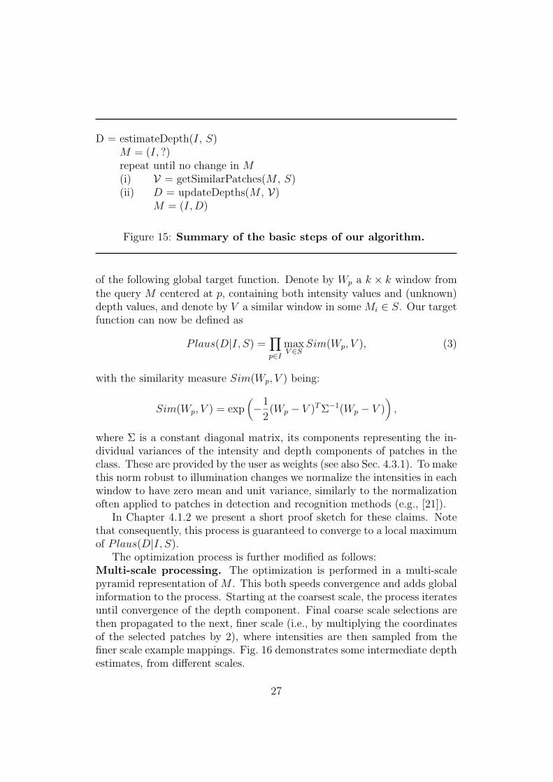
D = estimateDepth(I, S)M = (I, ?)repeat until no change in M(i) V = getSimilarPatches(M , S)(ii) D = updateDepths(M , V)

M = (I,D)

Figure 15: Summary of the basic steps of our algorithm.

of the following global target function. Denote by Wp a k × k window fromthe query M centered at p, containing both intensity values and (unknown)depth values, and denote by V a similar window in some Mi ∈ S. Our targetfunction can now be defined as

Plaus(D|I, S) =∏p∈I

maxV ∈S

Sim(Wp, V ), (3)

with the similarity measure Sim(Wp, V ) being:

Sim(Wp, V ) = exp(−1

2(Wp − V )T Σ−1(Wp − V )

),

where Σ is a constant diagonal matrix, its components representing the in-dividual variances of the intensity and depth components of patches in theclass. These are provided by the user as weights (see also Sec. 4.3.1). To makethis norm robust to illumination changes we normalize the intensities in eachwindow to have zero mean and unit variance, similarly to the normalizationoften applied to patches in detection and recognition methods (e.g., [21]).

In Chapter 4.1.2 we present a short proof sketch for these claims. Notethat consequently, this process is guaranteed to converge to a local maximumof Plaus(D|I, S).

The optimization process is further modified as follows:Multi-scale processing. The optimization is performed in a multi-scalepyramid representation of M . This both speeds convergence and adds globalinformation to the process. Starting at the coarsest scale, the process iteratesuntil convergence of the depth component. Final coarse scale selections arethen propagated to the next, finer scale (i.e., by multiplying the coordinatesof the selected patches by 2), where intensities are then sampled from thefiner scale example mappings. Fig. 16 demonstrates some intermediate depthestimates, from different scales.

27

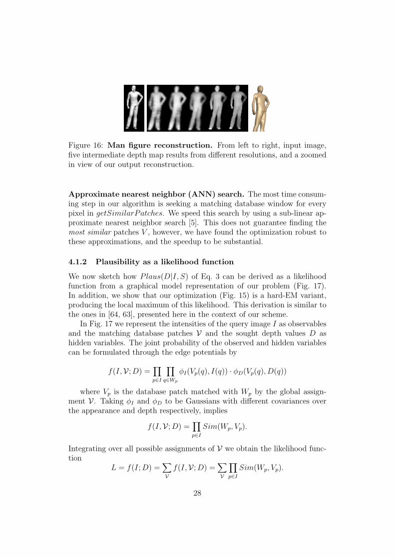
Figure 16: Man figure reconstruction. From left to right, input image,five intermediate depth map results from different resolutions, and a zoomedin view of our output reconstruction.

Approximate nearest neighbor (ANN) search. The most time consum-ing step in our algorithm is seeking a matching database window for everypixel in getSimilarPatches. We speed this search by using a sub-linear ap-proximate nearest neighbor search [5]. This does not guarantee finding themost similar patches V , however, we have found the optimization robust tothese approximations, and the speedup to be substantial.

4.1.2 Plausibility as a likelihood function

We now sketch how Plaus(D|I, S) of Eq. 3 can be derived as a likelihoodfunction from a graphical model representation of our problem (Fig. 17).In addition, we show that our optimization (Fig. 15) is a hard-EM variant,producing the local maximum of this likelihood. This derivation is similar tothe ones in [64, 63], presented here in the context of our scheme.

In Fig. 17 we represent the intensities of the query image I as observablesand the matching database patches V and the sought depth values D ashidden variables. The joint probability of the observed and hidden variablescan be formulated through the edge potentials by

f(I,V ; D) =∏p∈I

∏q∈Wp

φI(Vp(q), I(q)) · φD(Vp(q), D(q))

where Vp is the database patch matched with Wp by the global assign-ment V . Taking φI and φD to be Gaussians with different covariances overthe appearance and depth respectively, implies

f(I,V ; D) =∏p∈I

Sim(Wp, Vp).

Integrating over all possible assignments of V we obtain the likelihood func-tion

L = f(I; D) =∑V

f(I,V ; D) =∑V

∏p∈I

Sim(Wp, Vp).

28

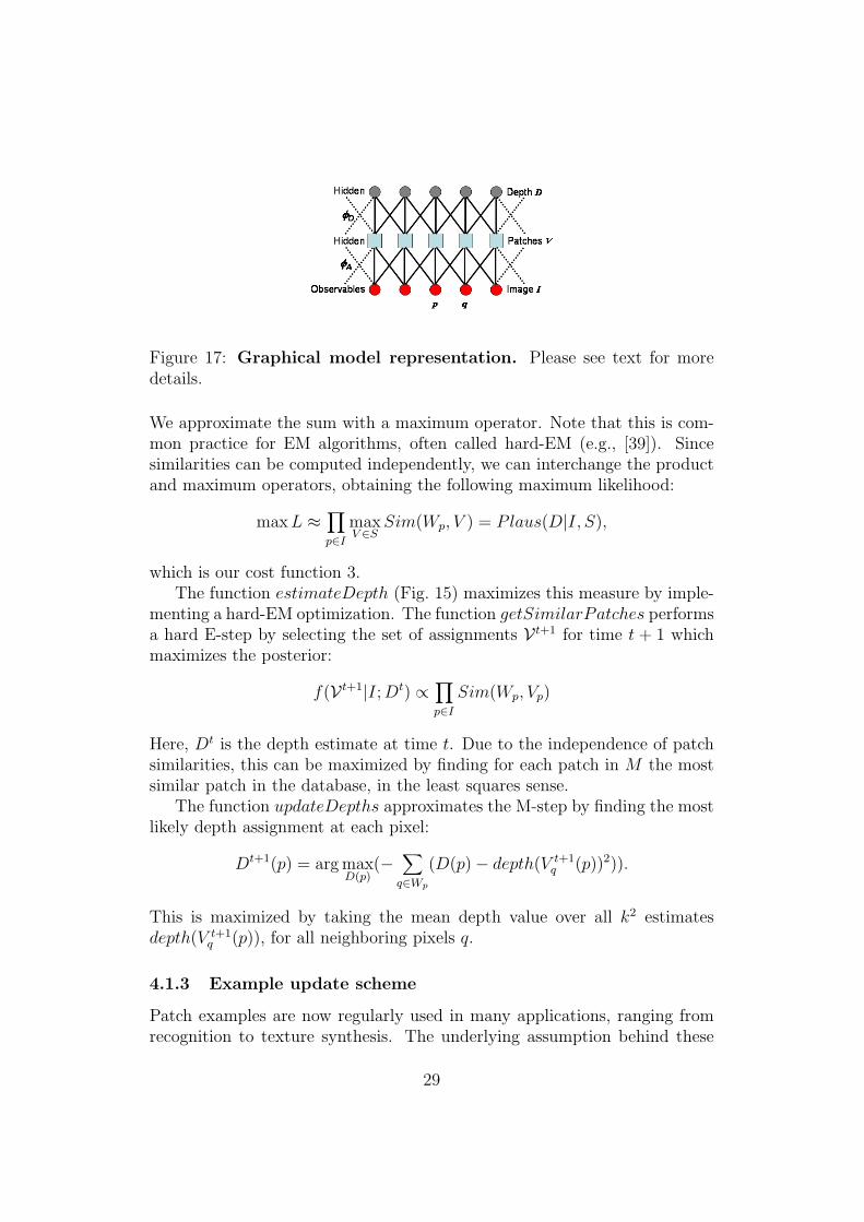
Figure 17: Graphical model representation. Please see text for moredetails.

We approximate the sum with a maximum operator. Note that this is com-mon practice for EM algorithms, often called hard-EM (e.g., [39]). Sincesimilarities can be computed independently, we can interchange the productand maximum operators, obtaining the following maximum likelihood:

max L ≈∏p∈I

maxV ∈S

Sim(Wp, V ) = Plaus(D|I, S),

which is our cost function 3.The function estimateDepth (Fig. 15) maximizes this measure by imple-

menting a hard-EM optimization. The function getSimilarPatches performsa hard E-step by selecting the set of assignments V t+1 for time t + 1 whichmaximizes the posterior:

f(V t+1|I; Dt) ∝∏p∈I

Sim(Wp, Vp)

Here, Dt is the depth estimate at time t. Due to the independence of patchsimilarities, this can be maximized by finding for each patch in M the mostsimilar patch in the database, in the least squares sense.

The function updateDepths approximates the M-step by finding the mostlikely depth assignment at each pixel:

Dt+1(p) = arg maxD(p)

(−∑

q∈Wp

(D(p)− depth(V t+1q (p))2)).

This is maximized by taking the mean depth value over all k2 estimatesdepth(V t+1

q (p)), for all neighboring pixels q.

4.1.3 Example update scheme

Patch examples are now regularly used in many applications, ranging fromrecognition to texture synthesis. The underlying assumption behind these

29

methods is that class variability can be captured by a finite, often small,set of examples. This is often true, but when the class contains non-rigidobjects, objects varying in texture, or when viewing conditions are allowedto change, this can become a problem. Adding more examples to allow formore variability (e.g.,rotations of the input image in [18]), implies largerstorage requirements, longer running times, and higher risk of false matches.In this work, we handle non-rigid objects (e.g.,hands), objects which varyin texture (e.g.,the fish) and can be viewed from any direction. Ideally, wewould like our examples to be objects whose shape is similar to that of theobject in the input image, viewed under similar conditions. This, however,implies a chicken-and-egg problem as reconstruction requires choosing similarobjects for our database, but for this we first need a reconstruction.

We thus propose the idea of online example set update. Instead of com-mitting to a fixed database at the onset of reconstruction, we propose up-dating the database on-the-fly during processing. We start with an initialseed database of examples. In subsequent iterations of our optimization wedrop the least used examples Mi from our database, replacing them withones deemed better for the reconstruction. These are produced by on-the-flyrendering of more suitable 3D objects with better viewing conditions. Inour experiments, we applied this idea to search for better example objectsand better viewing angles. Other parameters such as lighting conditions canbe similarly resolved. Note that this implies a potentially infinite exampledatabase (e.g.,infinite views), where only a small relevant subset is used atany one time. We next describe the details of our implementation.

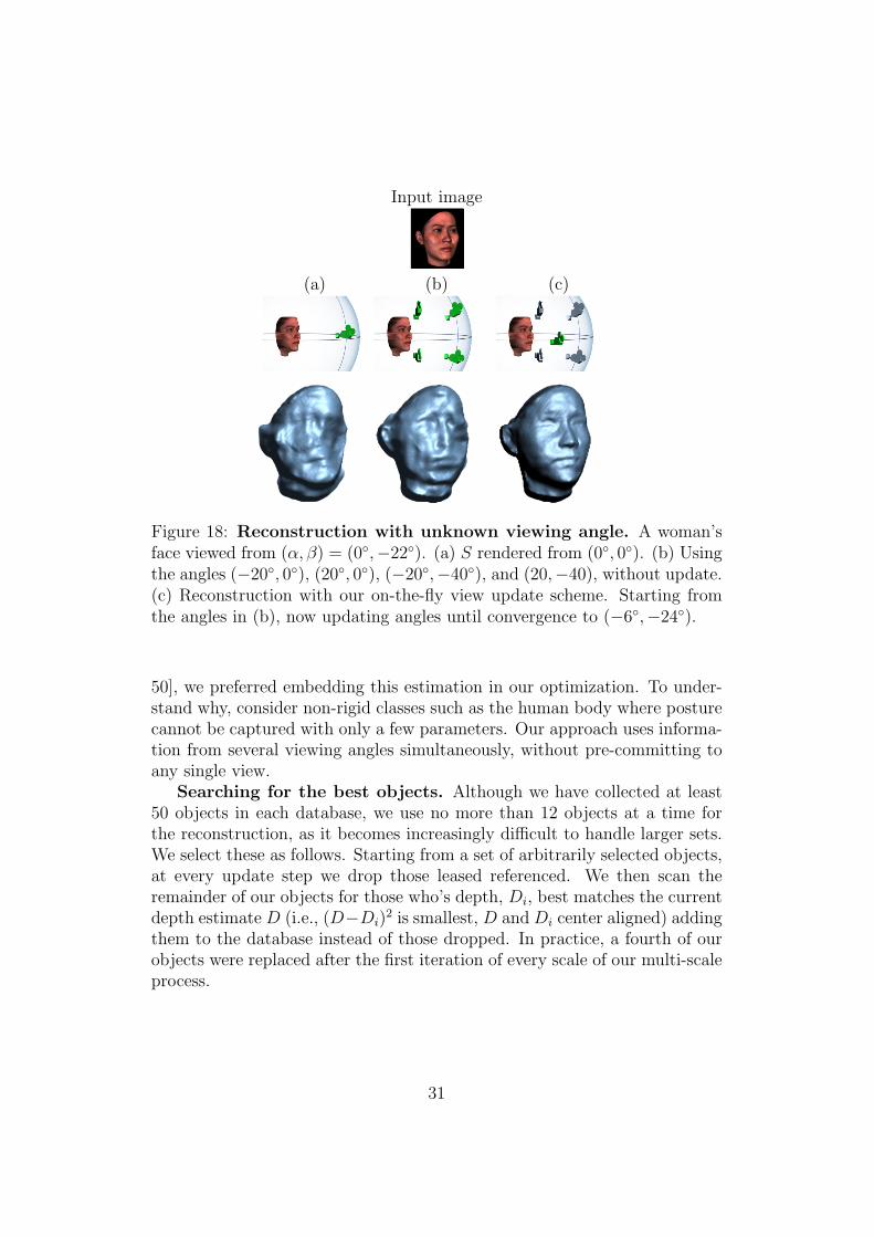
Searching for the best views. Fig. 18 demonstrates a reconstructionusing images from a single incorrect viewing angle (Fig. 18.a) and four fixedwidely spaced viewing angles (Fig. 18.b). Both are inadequate. It standsto reason that mappings from viewing angles closer to the real one, willcontribute more patches to the process than those further away. We thusadopt the following scheme. We start with a small number of pre-selectedviews, sparsely covering parts of the viewing sphere (the gray cameras inFig. 18.c). The seed database S is produced by taking the mappings Mi

of our objects, rendered from these views, and is used to obtain an initialdepth estimate. In subsequent iterations, we re-estimate our views by takingthe mean of the currently used angles, weighted by the relative number ofpatches selected from each angle. We then drop from S mappings originatingfrom the least used angle, and replace them with ones from the new view. Ifthe new view is sufficiently close to one of the remaining angles, we insteadincrease the number of objects to maintain the size of S. Fig. 18.c presentsa result obtained with our angle update scheme.

Although methods exist which accurately estimate the viewing angle [46,

30

Input image

(a) (b) (c)

Figure 18: Reconstruction with unknown viewing angle. A woman’sface viewed from (α, β) = (0◦,−22◦). (a) S rendered from (0◦, 0◦). (b) Usingthe angles (−20◦, 0◦), (20◦, 0◦), (−20◦,−40◦), and (20,−40), without update.(c) Reconstruction with our on-the-fly view update scheme. Starting fromthe angles in (b), now updating angles until convergence to (−6◦,−24◦).

50], we preferred embedding this estimation in our optimization. To under-stand why, consider non-rigid classes such as the human body where posturecannot be captured with only a few parameters. Our approach uses informa-tion from several viewing angles simultaneously, without pre-committing toany single view.

Searching for the best objects. Although we have collected at least50 objects in each database, we use no more than 12 objects at a time forthe reconstruction, as it becomes increasingly difficult to handle larger sets.We select these as follows. Starting from a set of arbitrarily selected objects,at every update step we drop those leased referenced. We then scan theremainder of our objects for those who’s depth, Di, best matches the currentdepth estimate D (i.e., (D−Di)

2 is smallest, D and Di center aligned) addingthem to the database instead of those dropped. In practice, a fourth of ourobjects were replaced after the first iteration of every scale of our multi-scaleprocess.

31

(a) (b) (c)

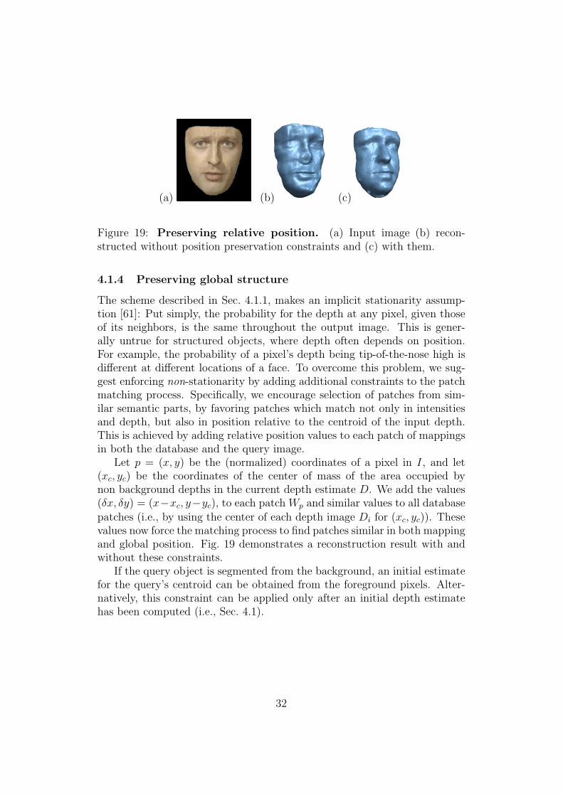
Figure 19: Preserving relative position. (a) Input image (b) recon-structed without position preservation constraints and (c) with them.

4.1.4 Preserving global structure

The scheme described in Sec. 4.1.1, makes an implicit stationarity assump-tion [61]: Put simply, the probability for the depth at any pixel, given thoseof its neighbors, is the same throughout the output image. This is gener-ally untrue for structured objects, where depth often depends on position.For example, the probability of a pixel’s depth being tip-of-the-nose high isdifferent at different locations of a face. To overcome this problem, we sug-gest enforcing non-stationarity by adding additional constraints to the patchmatching process. Specifically, we encourage selection of patches from sim-ilar semantic parts, by favoring patches which match not only in intensitiesand depth, but also in position relative to the centroid of the input depth.This is achieved by adding relative position values to each patch of mappingsin both the database and the query image.

Let p = (x, y) be the (normalized) coordinates of a pixel in I, and let(xc, yc) be the coordinates of the center of mass of the area occupied bynon background depths in the current depth estimate D. We add the values(δx, δy) = (x−xc, y−yc), to each patch Wp and similar values to all databasepatches (i.e., by using the center of each depth image Di for (xc, yc)). Thesevalues now force the matching process to find patches similar in both mappingand global position. Fig. 19 demonstrates a reconstruction result with andwithout these constraints.

If the query object is segmented from the background, an initial estimatefor the query’s centroid can be obtained from the foreground pixels. Alter-natively, this constraint can be applied only after an initial depth estimatehas been computed (i.e., Sec. 4.1).

32

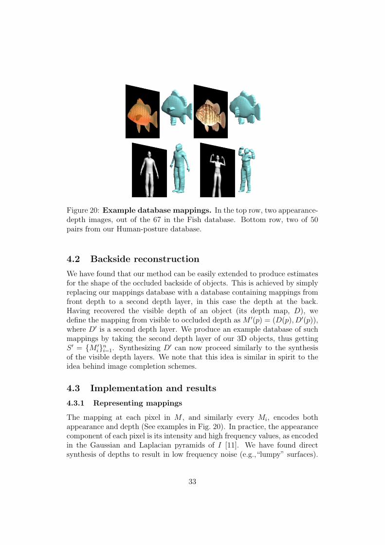
Figure 20: Example database mappings. In the top row, two appearance-depth images, out of the 67 in the Fish database. Bottom row, two of 50pairs from our Human-posture database.

4.2 Backside reconstruction

We have found that our method can be easily extended to produce estimatesfor the shape of the occluded backside of objects. This is achieved by simplyreplacing our mappings database with a database containing mappings fromfront depth to a second depth layer, in this case the depth at the back.Having recovered the visible depth of an object (its depth map, D), wedefine the mapping from visible to occluded depth as M ′(p) = (D(p), D′(p)),where D′ is a second depth layer. We produce an example database of suchmappings by taking the second depth layer of our 3D objects, thus gettingS ′ = {M ′

i}ni=1. Synthesizing D′ can now proceed similarly to the synthesis

of the visible depth layers. We note that this idea is similar in spirit to theidea behind image completion schemes.

4.3 Implementation and results

4.3.1 Representing mappings

The mapping at each pixel in M , and similarly every Mi, encodes bothappearance and depth (See examples in Fig. 20). In practice, the appearancecomponent of each pixel is its intensity and high frequency values, as encodedin the Gaussian and Laplacian pyramids of I [11]. We have found directsynthesis of depths to result in low frequency noise (e.g.,“lumpy” surfaces).

33

We thus estimate a Laplacian pyramid of the depth instead, producing thefinal depth by collapsing the depth estimates from all scales. In this fashion,low frequency depths are synthesized in the course scale of the pyramid andonly sharpened at finer scales.

Different patch components, including relative positions, contribute dif-ferent amounts of information in different classes, as reflected by their differ-ent variance. For example, faces are highly structured, thus, position playsan important role in their reconstruction. On the other hand, due to thevariability of human postures, relative position is less reliable for that class.We therefore amplify different components of each Wp for different classes,by weighting them differently. We use four weights, one for each of the twoappearance components, one for depth, and one for relative position. Theseweights were set once for each object class, and changed only if the querywas significantly different from the images in S.

4.3.2 Implementation

Our algorithm was implemented in MATLAB, except for the ANN code [5],which was used as a stand alone executable. We experimented with thefollowing data sets. Hand and body objects, produced by exporting built-inmodels from the Poser 6 software, the USF head database [59], and a fishdatabase [56]. Our objects are stored as textured 3D models. We can thusrender them to produce example mappings using any standard renderingengine. Example mappings from the fish and human posture data-sets aredisplayed in Fig. 20. We used 3D Studio Max for rendering. We preferred pre-rendering the images and depth maps instead of rendering different objectsfrom different angles on-the-fly. Thus, we trade rendering times with diskaccess times and large storage. Note that this is an implementation decision;at any one time we load only a small number of images to memory. Theangle update step (Sec. 4.1.3) therefore selects the existing pre-rendered angleclosest to the mean angle.

4.3.3 Experiments

We found the algorithm to perform well on structured rigid objects, such asfaces. However, hands, having little texture and varying greatly in shape,proved more difficult, requiring more parameter manipulations. In generalthe success of a reconstruction relies on the database used, the input image,and how the two match (some failed results are presented in Fig. 21). Resultsare shown in Figures 19, 18, 22– 25. In addition, Fig. 22 and 23 presentresults for the backside of imaged objects (i.e., Sec. 4.2). The query objectswere manually segmented from their background and then aligned with a

34

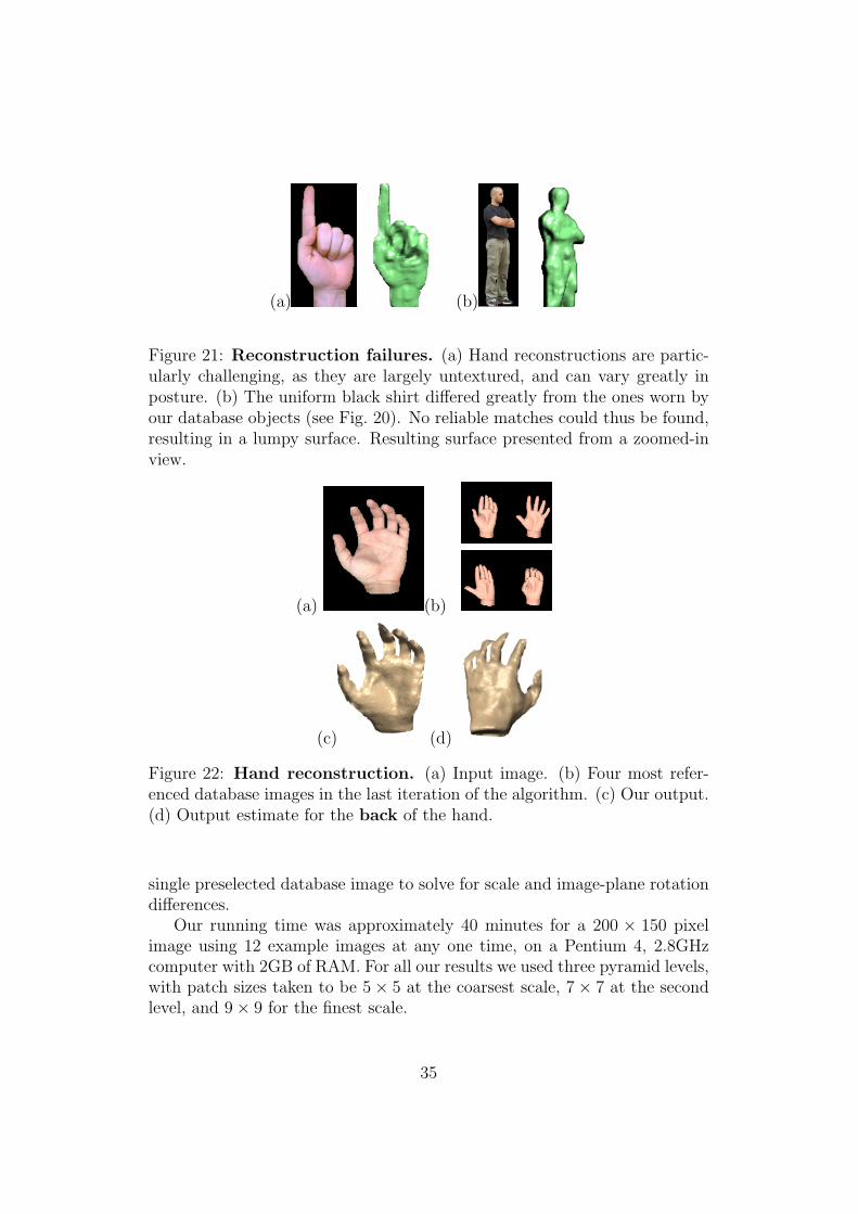
(a) (b)

Figure 21: Reconstruction failures. (a) Hand reconstructions are partic-ularly challenging, as they are largely untextured, and can vary greatly inposture. (b) The uniform black shirt differed greatly from the ones worn byour database objects (see Fig. 20). No reliable matches could thus be found,resulting in a lumpy surface. Resulting surface presented from a zoomed-inview.

(a) (b)

(c) (d)

Figure 22: Hand reconstruction. (a) Input image. (b) Four most refer-enced database images in the last iteration of the algorithm. (c) Our output.(d) Output estimate for the back of the hand.

single preselected database image to solve for scale and image-plane rotationdifferences.

Our running time was approximately 40 minutes for a 200 × 150 pixelimage using 12 example images at any one time, on a Pentium 4, 2.8GHzcomputer with 2GB of RAM. For all our results we used three pyramid levels,with patch sizes taken to be 5× 5 at the coarsest scale, 7× 7 at the secondlevel, and 9× 9 for the finest scale.

35

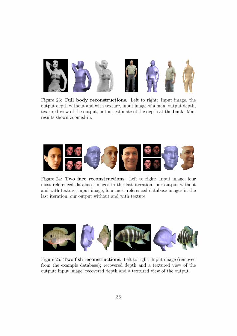
Figure 23: Full body reconstructions. Left to right: Input image, theoutput depth without and with texture, input image of a man, output depth,textured view of the output, output estimate of the depth at the back. Manresults shown zoomed-in.

Figure 24: Two face reconstructions. Left to right: Input image, fourmost referenced database images in the last iteration, our output withoutand with texture, input image, four most referenced database images in thelast iteration, our output without and with texture.

Figure 25: Two fish reconstructions. Left to right: Input image (removedfrom the example database); recovered depth and a textured view of theoutput; Input image; recovered depth and a textured view of the output.

36

5 Automatic Depth-Map Colorization

Our automatic depth-map colorization method [26] is closely related to thedepth reconstruction method described in Chapter 4. In particular, the twomethods share the same optimization scheme. In the following chpter wehighlight some of the differences between the two procedures.

5.1 Image-map synthesis

For a given depth D(x, y), we attempt to synthesize a matching image-mapI(x, y). To this end we use examples of feasible mappings from depths toimages of similar objects, stored in a database S = {Mi}n

i=1 = {(Di, Ii)}ni=1,

where Di and Ii respectively are the depth and image maps of exampleobjects. Our goal is to produce an image-map I such that M = (D, I)will also be feasible. Specifically, we seek an image I which will satisfy thefollowing criteria: (i) For every k × k patch of mappings in M , there is asimilar patch in S. (ii) Database patches matched with overlapping patchesin M , will agree on the colors I(p), at overlapped pixels p = (x, y). Wenote that our goal here is the reverse of the one behind our reconstructionframework (Chapter 4 and [27]). There, the input is an image I and theoutput is a depth-map D (whereas here it is the opposite). Similarly, thedatabase S for reconstruction contains image-depth pairs, where here westore depth-image pairs.

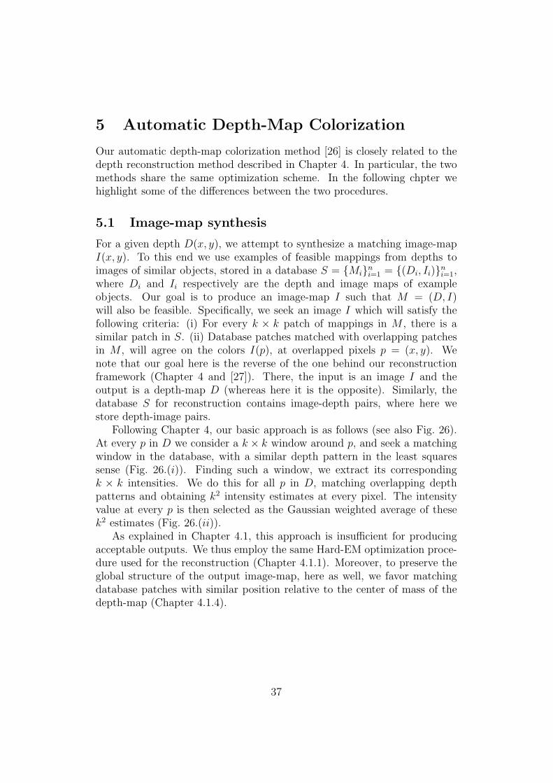
Following Chapter 4, our basic approach is as follows (see also Fig. 26).At every p in D we consider a k × k window around p, and seek a matchingwindow in the database, with a similar depth pattern in the least squaressense (Fig. 26.(i)). Finding such a window, we extract its correspondingk × k intensities. We do this for all p in D, matching overlapping depthpatterns and obtaining k2 intensity estimates at every pixel. The intensityvalue at every p is then selected as the Gaussian weighted average of thesek2 estimates (Fig. 26.(ii)).

As explained in Chapter 4.1, this approach is insufficient for producingacceptable outputs. We thus employ the same Hard-EM optimization proce-dure used for the reconstruction (Chapter 4.1.1). Moreover, to preserve theglobal structure of the output image-map, here as well, we favor matchingdatabase patches with similar position relative to the center of mass of thedepth-map (Chapter 4.1.4).

37

Figure 26: Image-map synthesis. Step (i) finds for every query patch asimilar database patch. Overlapping patches provide color estimates for theirpixels. (ii) These estimates are averaged to determine the color at each pixel.

5.2 Accelerating synthesis

Our colorization scheme was designed with the intention of allowing multi-tudes of depth-maps to be rapidly colorized. The running times measuredfor our reconstruction framework, as reported in Chapter 4.3.3, were thusunacceptable. The basic scheme used in both reconstruction and coloriza-tion, was therefore improved in the following two ways, in an attempt tosignificantly reduce running times.

Partial databases. Although over 50 mappings Mi were collected forsome of our sets S, in practice, we use only small subsets of these databases.Selecting the mappings Mi used for each synthesis depends on the modeler’sintentions, as follows. (a) For automatic \ mass image-map production, atthe onset of synthesis, we automatically choose the m mappings Mi with themost similar depth-map to D (i.e., (D−Di)

2 is minimal, D and Di centroidaligned), where normally m << |S|. (b) Alternatively, our system allows themodeler to manually select specific mappings with desired image-maps.

PCA patches. Before the first matching process of each scale com-mences, separate PCA transformation matrices are learned from the depthand intensity bands of the database subset used for synthesis. In practice,we keep a fifth of the basis vectors with the highest variance. The matchingprocess thus finds the most similar PCA reduced patches in the database.This provides a speedup factor of about 5, by loosing some information,however, in all our tests this did not seem to effect the quality of our results.

38

5.3 Implementation and results

5.3.1 Representation of Examples

The depth component of each Mi and similarly M is taken to be the depthitself and its high frequency values, as encoded in the Gaussian and Laplacianpyramids of D. We synthesize three Laplacian pyramids for each of theYCbCr bands of the image-map. The final result is produced by collapsingthese pyramids. Consequently, a low frequency image-map is synthesizedat the course scale of the pyramid and only refined and sharpened at finerscales.

Different patch components contribute different amounts of informationin different classes, as reflected by their different variance. The modeler canthus amplify different components of each Wp by weighting them differently.We use 6 weights, one for each of the two depth components, three for theYCbCr bands, and one for relative position. Although selected manually,these weights were set once for each object class, and left unchanged in allour experiments.

5.3.2 Implementation

Our algorithm was implemented in MATLAB, except for the ANN code,which was used as a stand alone executable. Our data sets were 5 humanobjects courtesy of Cyberware Inc., 76 busts from [59], and 57 fish objectsfrom [56]. We assume that test depths are aligned with depths in the data-base. If not, depths can be aligned using, e.g., [43].

5.3.3 Experiments

We ran leave-one-out tests on all three data sets, automatically selectingdatabase examples for each synthesis. Parameters are reported in Table 2.Some results are presented in Fig. 27-31. To evaluate the quality of ourresults, we have poled 10 subjects, asking “how many image-maps are faultyor otherwise inferior to those in the database”. 28% and 24% faults werecounted on average in the Fish and Face databases, respectively. Note againthat no parameter optimization was carried out for individual depths. With5 shapes, the humans set was too small for statistics.

Our average running time using un-optimized code, was approximately71

2minutes for 200 × 150 pixel images using m = 2 examples of similar

dimensions, on a Pentium 4, 2.8GHz computer with 2GB of RAM.

39

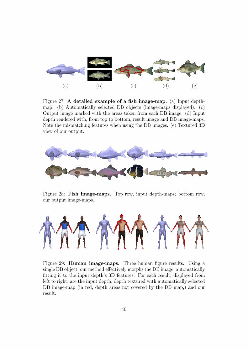
(a) (b) (c) (d) (e)

Figure 27: A detailed example of a fish image-map. (a) Input depth-map. (b) Automatically selected DB objects (image-maps displayed). (c)Output image marked with the areas taken from each DB image. (d) Inputdepth rendered with, from top to bottom, result image and DB image-maps.Note the mismatching features when using the DB images. (e) Textured 3Dview of our output.

Figure 28: Fish image-maps. Top row, input depth-maps; bottom row,our output image-maps.

Figure 29: Human image-maps. Three human figure results. Using asingle DB object, our method effectively morphs the DB image, automaticallyfitting it to the input depth’s 3D features. For each result, displayed fromleft to right, are the input depth, depth textured with automatically selectedDB image-map (in red, depth areas not covered by the DB map,) and ourresult.

40

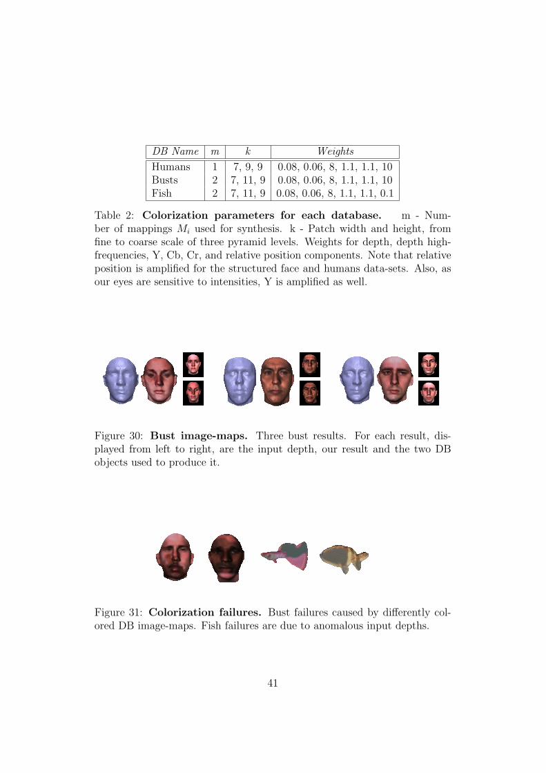
DB Name m k Weights

Humans 1 7, 9, 9 0.08, 0.06, 8, 1.1, 1.1, 10Busts 2 7, 11, 9 0.08, 0.06, 8, 1.1, 1.1, 10Fish 2 7, 11, 9 0.08, 0.06, 8, 1.1, 1.1, 0.1

Table 2: Colorization parameters for each database. m - Num-ber of mappings Mi used for synthesis. k - Patch width and height, fromfine to coarse scale of three pyramid levels. Weights for depth, depth high-frequencies, Y, Cb, Cr, and relative position components. Note that relativeposition is amplified for the structured face and humans data-sets. Also, asour eyes are sensitive to intensities, Y is amplified as well.

Figure 30: Bust image-maps. Three bust results. For each result, dis-played from left to right, are the input depth, our result and the two DBobjects used to produce it.

Figure 31: Colorization failures. Bust failures caused by differently col-ored DB image-maps. Fish failures are due to anomalous input depths.

41

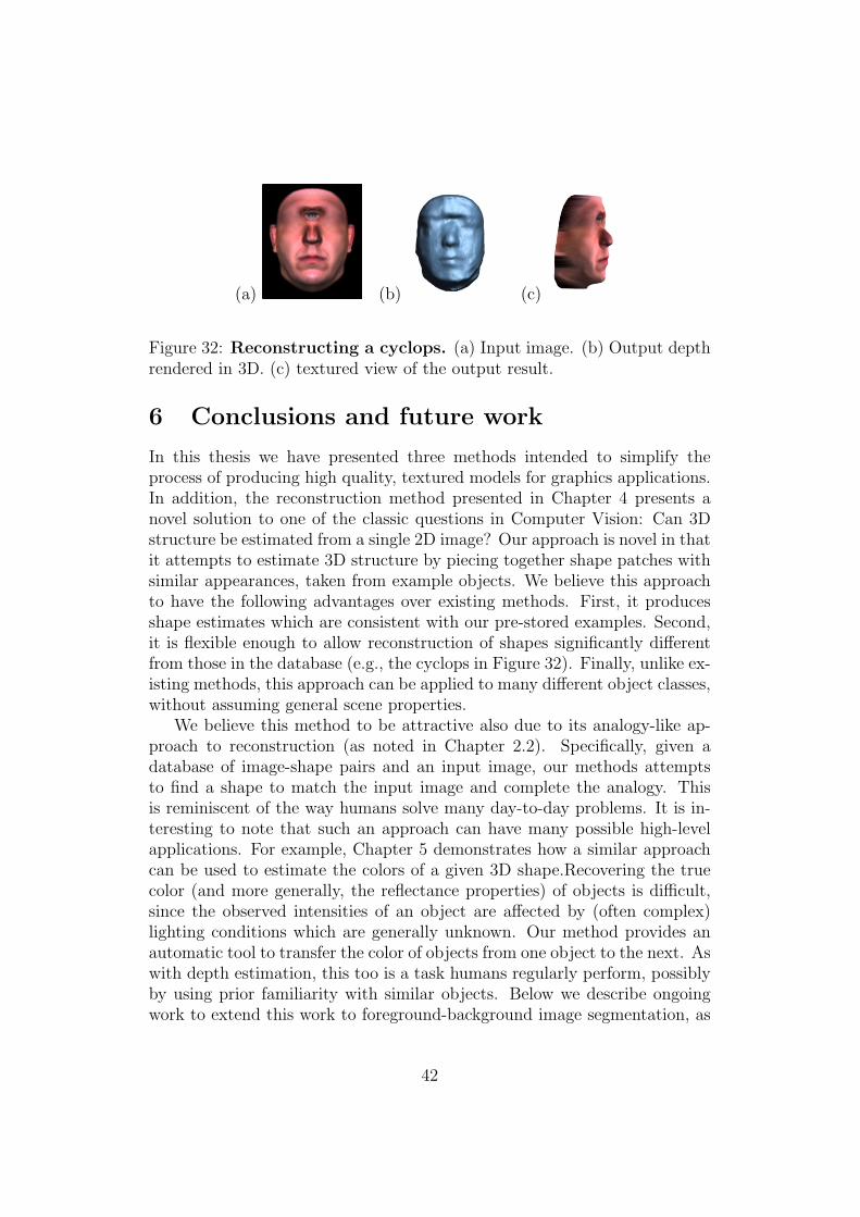
(a) (b) (c)

Figure 32: Reconstructing a cyclops. (a) Input image. (b) Output depthrendered in 3D. (c) textured view of the output result.

6 Conclusions and future work

In this thesis we have presented three methods intended to simplify theprocess of producing high quality, textured models for graphics applications.In addition, the reconstruction method presented in Chapter 4 presents anovel solution to one of the classic questions in Computer Vision: Can 3Dstructure be estimated from a single 2D image? Our approach is novel in thatit attempts to estimate 3D structure by piecing together shape patches withsimilar appearances, taken from example objects. We believe this approachto have the following advantages over existing methods. First, it producesshape estimates which are consistent with our pre-stored examples. Second,it is flexible enough to allow reconstruction of shapes significantly differentfrom those in the database (e.g., the cyclops in Figure 32). Finally, unlike ex-isting methods, this approach can be applied to many different object classes,without assuming general scene properties.

We believe this method to be attractive also due to its analogy-like ap-proach to reconstruction (as noted in Chapter 2.2). Specifically, given adatabase of image-shape pairs and an input image, our methods attemptsto find a shape to match the input image and complete the analogy. Thisis reminiscent of the way humans solve many day-to-day problems. It is in-teresting to note that such an approach can have many possible high-levelapplications. For example, Chapter 5 demonstrates how a similar approachcan be used to estimate the colors of a given 3D shape.Recovering the truecolor (and more generally, the reflectance properties) of objects is difficult,since the observed intensities of an object are affected by (often complex)lighting conditions which are generally unknown. Our method provides anautomatic tool to transfer the color of objects from one object to the next. Aswith depth estimation, this too is a task humans regularly perform, possiblyby using prior familiarity with similar objects. Below we describe ongoingwork to extend this work to foreground-background image segmentation, as

42

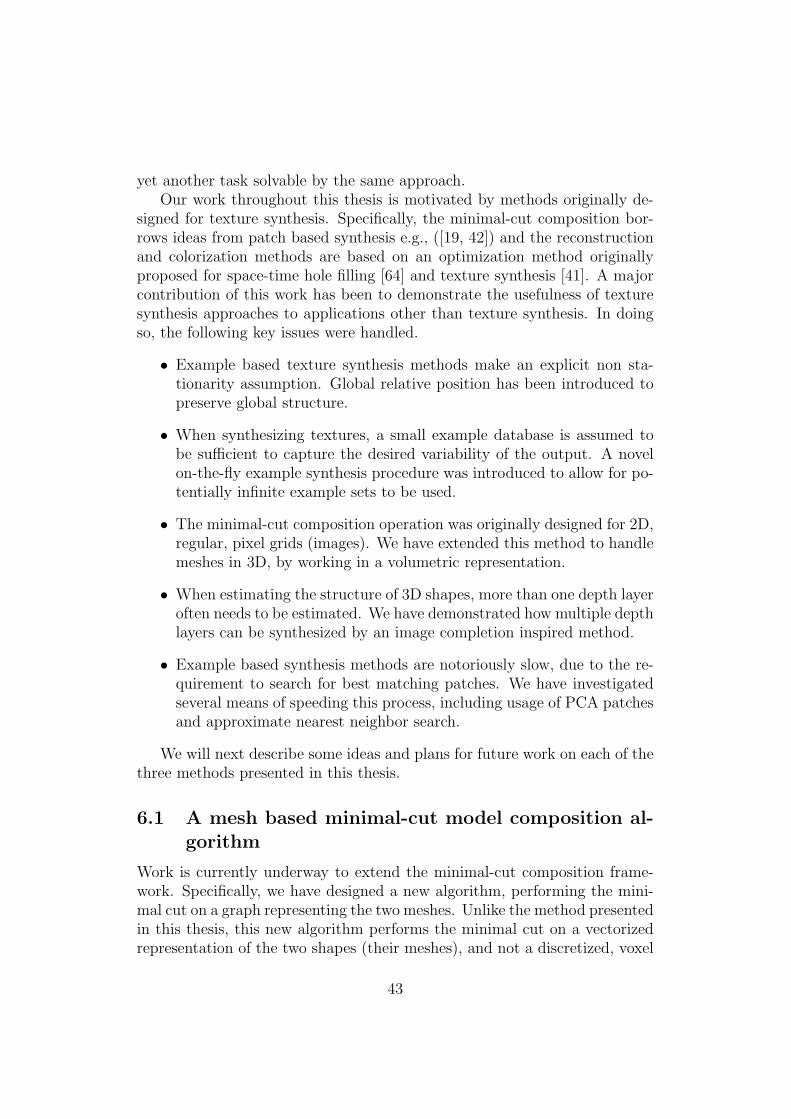
yet another task solvable by the same approach.Our work throughout this thesis is motivated by methods originally de-

signed for texture synthesis. Specifically, the minimal-cut composition bor-rows ideas from patch based synthesis e.g., ([19, 42]) and the reconstructionand colorization methods are based on an optimization method originallyproposed for space-time hole filling [64] and texture synthesis [41]. A majorcontribution of this work has been to demonstrate the usefulness of texturesynthesis approaches to applications other than texture synthesis. In doingso, the following key issues were handled.

• Example based texture synthesis methods make an explicit non sta-tionarity assumption. Global relative position has been introduced topreserve global structure.

• When synthesizing textures, a small example database is assumed tobe sufficient to capture the desired variability of the output. A novelon-the-fly example synthesis procedure was introduced to allow for po-tentially infinite example sets to be used.

• The minimal-cut composition operation was originally designed for 2D,regular, pixel grids (images). We have extended this method to handlemeshes in 3D, by working in a volumetric representation.

• When estimating the structure of 3D shapes, more than one depth layeroften needs to be estimated. We have demonstrated how multiple depthlayers can be synthesized by an image completion inspired method.

• Example based synthesis methods are notoriously slow, due to the re-quirement to search for best matching patches. We have investigatedseveral means of speeding this process, including usage of PCA patchesand approximate nearest neighbor search.

We will next describe some ideas and plans for future work on each of thethree methods presented in this thesis.

6.1 A mesh based minimal-cut model composition al-gorithm

Work is currently underway to extend the minimal-cut composition frame-work. Specifically, we have designed a new algorithm, performing the mini-mal cut on a graph representing the two meshes. Unlike the method presentedin this thesis, this new algorithm performs the minimal cut on a vectorizedrepresentation of the two shapes (their meshes), and not a discretized, voxel

43

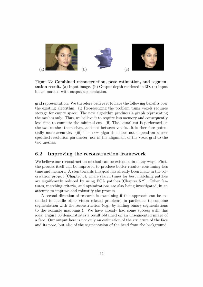
(a) (b) (c)

Figure 33: Combined reconstruction, pose estimation, and segmen-tation result. (a) Input image. (b) Output depth rendered in 3D. (c) Inputimage masked with output segmentation.

grid representation. We therefore believe it to have the following benefits overthe existing algorithm. (i) Representing the problem using voxels requiresstorage for empty space. The new algorithm produces a graph representingthe meshes only. Thus, we believe it to require less memory and consequentlyless time to compute the minimal-cut. (ii) The actual cut is performed onthe two meshes themselves, and not between voxels. It is therefore poten-tially more accurate. (iii) The new algorithm does not depend on a userspecified resolution parameter, nor in the alignment of the voxel grid to thetwo meshes.

6.2 Improving the reconstruction framework

We believe our reconstruction method can be extended in many ways. First,the process itself can be improved to produce better results, consuming lesstime and memory. A step towards this goal has already been made in the col-orization project (Chapter 5), where search times for best matching patchesare significantly reduced by using PCA patches (Chapter 5.2). Other fea-tures, matching criteria, and optimizations are also being investigated, in anattempt to improve and robustify the process.

A second direction of research is examining if this approach can be ex-tended to handle other vision related problems, in particular to combinesegmentation with the reconstruction (e.g., by adding binary segmentationsto the example mappings.). We have already had some success with thisidea. Figure 33 demonstrates a result obtained on an unsegmented image ofa face. Our output here is not only an estimation of the structure of the faceand its pose, but also of the segmentation of the head from the background.

44

6.3 Automatic mesh colorization

The method presented here automatically produces image-maps for 3D ob-jects represented as depth-maps. A more useful and common representationfor 3D models is triangulated meshes. We are therefore concentrating onporting our method to meshes. We note that the optimization used in ourwork has already been extended to produce textures on surfaces in [25].Their system, however, takes as input a texture sample (an image) and a3D shape. It then produces an image map for the shape by synthesizing thetexture sample on the surface. Our goal, on the other hand is to design asystem capable of taking parts of the image-maps of sample 3D objects andcombining them to produce a novel structured image-map for an input 3Dobject. We believe this to be a non trivial extension of both our currentwork, and theirs.

45

References

[1] B. Adams and P. Dutre. Interactive boolean operations on surfel-bounded solids. ACM Trans. Graph., 22(3):651–656, 2003.

[2] A. Agarwala, M. Dontcheva, M. Agrawala, S. Drucker, A. Colburn,B. Curless, D. Salesin, and M. Cohen. Interactive digital photomon-tage. ACM Trans. Graph., 23(3):294–302, 2004.

[3] M. Alexa. Local control for mesh morphing. In SMI ’01: Proceedings ofthe International Conference on Shape Modeling & Applications, page209. IEEE Computer Society, 2001.

[4] B. Allen, B. Curless, and Z. Popovic. The space of all body shapes:Reconstruction and parameterization from range scans. ACM Trans.Graph., 22(3):587–594, 2003.

[5] S. Arya, D.M. Mount, N.S. Netanyahu, R. Silverman, and A.Y. Wu. Anoptimal algorithm for approximate nearest neighbor searching in fixeddimensions. Journal of the ACM, 45(6):891–923, 1998. Source codeavailable from www.cs.umd.edu/∼mount/ANN/.

[6] J.J. Atick, P.A. Griffin, and A.N. Redlich. Statistical approach to shapefrom shading: Reconstruction of three-dimensional face surfaces fromsingle two-dimensional images. Neural Computation, 8(6):1321–1340,1996.

[7] H. Biermann, D. Kristjansson, and D. Zorin. Approximate booleanoperations on free-form solids. In SIGGRAPH ’01: Proceedings of the28th annual conference on Computer graphics and interactive techniques,pages 185–194. ACM Press, 2001.

[8] H. Biermann, I. Martin, F. Bernardini, and D. Zorin. Cut-and-pasteediting of multiresolution subdivision surfaces. ACM Trans. Graph.,21(3):312–321, 2002.

[9] V. Blanz and T. Vetter. A morphable model for the synthesis of 3Dfaces. In SIGGRAPH ’99: Proceedings of the 26th annual conferenceon Computer graphics and interactive techniques, pages 187–194. ACMPress/Addison-Wesley Publishing Co., 1999.

[10] Y. Boykov and V. Kolmogorov. An experimental comparison of min-cut/max-flow algorithms for energy minimization in vision. IEEE Trans.on Pattern Analysis and Machine Intelligence, 26(9):1124–1137, 2004.

[11] P. Burt and E. Adelson. The laplacian pyramid as a compact imagecode. In IEEE Trans. on Communications, volume 30, pages 532–540,April 1983.

[12] M. Cavazza, R. Earnshaw, N. Magnenat-Thalmann, and D. Thalmann.Survey: Motion control of virtual humans. IEEE Computer Graphics &Applications, 18(5):24–31, 1998.

[13] R. Cipolla, G.J. Fletcher, and P.J. Giblin. Surface geometry from cuspsof apparent contours. In Int. Conf. on Computer Vision, pages 858–863,1995.

[14] D. Cohen. Voxel traversal along a 3D line. Graphics gems IV, pages366–369, 1994.

[15] A. Criminisi, I. Reid, and A. Zisserman. Single view metrology. Inter-national Journal of Computer Vision, 40(2):123–148, November 2000.

[16] J. Davis, S.R. Marschner, M. Garr, and M. Levoy. Filling holes incomplex surfaces using volumetric diffusion. In Proc. Int. Symp. on 3DData Processing, Visualization, 2002.

[17] R. Dovgard and R. Basri. Statistical symmetric shape from shading for3D structure recovery of faces. In European Conf. on Computer Vision,volume 2, pages 99–113. Springer Berlin / Heidelberg, 2004.

[18] I. Drori, D. Cohen-Or, and H. Yeshurun. Fragment-based image com-pletion. ACM Trans. Graph., 22(3):303–312, 2003.

[19] A.A. Efros and W.T. Freeman. Image quilting for texture synthesis andtransfer. In SIGGRAPH ’01: Proceedings of the 28th annual conferenceon Computer graphics and interactive techniques, pages 341–346. ACMPress, 2001.

[20] A.A. Efros and T.K. Leung. Texture synthesis by non-parametric sam-pling. In Int. Conf. on Computer Vision, volume 2, pages 1033–1038,1999.

[21] R. Fergus, P. Perona, and A. Zisserman. A sparse object category modelfor efficient learning and exhaustive recognition. In IEEE Conf. on Com-puter Vision and Pattern Recognition, pages 380–387. IEEE ComputerSociety, 2005.

[22] L. Ford and D. Fulkerson. Flows in Networks. Princeton UniversityPress, 1962.

47

[23] T. Funkhouser, M. Kazhdan, P. Shilane, P. Min, W. Kiefer, A. Tal,S. Rusinkiewicz, and D. Dobkin. Modeling by example. ACM Trans.Graph., 23(3):652–663, 2004.

[24] F. Han and S.-C. Zhu. Bayesian reconstruction of 3D shapes and scenesfrom a single image. In HLK ’03: Proceedings of the First IEEE In-ternational Workshop on Higher-Level Knowledge in 3D Modeling andMotion Analysis, page 12. IEEE Computer Society, 2003.

[25] J. Han, K. Zhou, L. Wei, M. Gong, H. Bao, X. Zhang, and B. Guo. Fastexample-based surface texture synthesis via discrete optimization. InProc. of Pacific Graphics, 2006. Forthcoming.

[26] T. Hassner and R. Basri. Automatic depth-map colorization. In Euro-graphics (short), 2006. Forthcoming.

[27] T. Hassner and R. Basri. Example based 3D reconstruction from single2D images. In Beyond Patches Workshop at CVPR, page 15, June 2006.

[28] T. Hassner, L. Zelnik-Manor, G. Leifman, and R. Basri. Minimal-cutmodel composition. In International Conference on Shape Modeling andApplications (SMI’ 05), pages 72–81, June 2005.

[29] A. Hertzmann, C. Jacobs, N. Oliver, B. Curless, and D. Salesin. Imageanalogies. In SIGGRAPH ’01: Proceedings of the 28th annual conferenceon Computer graphics and interactive techniques, pages 327–340. ACMPress, 2001.

[30] C.M. Hoffmann. Geometric and solid modeling: an introduction. MorganKaufmann Publishers Inc., 1989.

[31] D. Hoiem, A.A. Efros, and M. Hebert. Automatic photo pop-up. ACMTrans. Graph., 24(3):577–584, 2005.

[32] D. Hoiem, A.A. Efros, and M. Hebert. Geometric context from a singleimage. In International Conference of Computer Vision (ICCV). IEEE,October 2005.

[33] B.K.P. Horn. Obtaining Shape from Shading Information. The Psychol-ogy of Computer Vision. McGraw-Hill, 1975.

[34] Z. Ji, L. Liu, Z. Chen, and G. Wang. Easy mesh cutting. In Proc. ofPacific Graphics, 2006. Forthcoming.

48

[35] J. Jia, J. Sun, C.-K. Tang, and H.-Y. Shum. Drag-and-drop pasting.ACM Trans. Graph., 25(3):631–637, 2006.

[36] I.T. Jolliffe. Principal Component Analysis. Springer-Verlag, New-York,1988.

[37] T. Kanai, H. Suzuki, J. Mitani, and F. Kimura. Interactive mesh fusionbased on local 3D metamorphosis. In Graphics Interface, pages 148–156,1999.

[38] S. Katz and A. Tal. Hierarchical mesh decomposition using fuzzy clus-tering and cuts. ACM Transactions on Graphics, 22(3):954–961, July2003.

[39] M.J. Kearns, Y. Mansour, and A.Y. Ng. An information-theoretic analy-sis of hard and soft assignment methods for clustering. In Proceedingsof the NATO Advanced Study Institute on Learning in graphical models,pages 495–520. Kluwer Academic Publishers, 1998.

[40] V. Kraevoy and A. Sheffer. Cross-parameterization and compatibleremeshing of 3d models. ACM Trans. Graph., 23(3):861–869, 2004.

[41] V. Kwatra, I. Essa, A. Bobick, and N. Kwatra. Texture optimizationfor example-based synthesis. ACM Trans. Graph., 24(3):795–802, 2005.

[42] V. Kwatra, A. Schodl, I. Essa, G. Turk, and A. Bobick. Graphcuttextures: image and video synthesis using graph cuts. ACM Trans.Graph., 22(3):277–286, 2003.

[43] A. Makadia, A. Patterson, and K. Daniilidis. Fully automatic registra-tion of 3D point clouds. In IEEE Conf. on Computer Vision and PatternRecognition, volume 1, pages 1297–1304. IEEE Computer Society, 2006.

[44] K. Museth, D. Breen, R. Whitaker, and Alan Barr. Level set surfaceediting operators. In SIGGRAPH ’02: Proceedings of the 29th annualconference on Computer graphics and interactive techniques, pages 330–338. ACM Press, 2002.

[45] B.M. Oh, M. Chen, J. Dorsey, and F. Durand. Image-based modelingand photo editing. In SIGGRAPH ’01: Proceedings of the 28th annualconference on Computer graphics and interactive techniques, pages 433–442. ACM Press, 2001.

49

[46] R. Osadchy, M. Miller, and Y. LeCun. Synergistic face detection andpose estimation with energy-based model. In Advances in Neural Infor-mation Processing Systems (NIPS 2004). MIT Press, 2005.

[47] M. Pauly, R. Keiser, L. Kobbelt, and M. Gross. Shape modeling withpoint-sampled geometry. ACM Trans. Graph., 22(3):641–650, 2003.

[48] E. Praun, W. Sweldens, and P. Schroder. Consistent mesh parameteri-zations. In SIGGRAPH ’01: Proceedings of the 28th annual conferenceon Computer graphics and interactive techniques, pages 179–184. ACMPress, 2001.

[49] K. Pulli and M. Ginzton. Scanalyze.http://graphics.stanford.edu/software/scanalyze, 2002.

[50] S. Romdhani, V. Blanz, and T. Vetter. Face identification by fitting a3d morphable model using linear shape and texture error functions. InECCV ’02: Proceedings of the 7th European Conference on ComputerVision, volume 4, pages 3–19. Springer-Verlag, 2002.

[51] S. Romdhani and T. Vetter. Efficient, robust and accurate fitting ofa 3D morphable model. In ICCV ’03: Proceedings of the Ninth IEEEInternational Conference on Computer Vision, page 59. IEEE ComputerSociety, 2003.

[52] S. Rusinkiewicz and M. Levoy. Efficient variants of the ICP algorithm.In Int. Conf. on 3-D Digital Imaging and Modeling (3DIM), page 145,2001.

[53] A. Sharf, M. Alexa, and D. Cohen-Or. Context-based surface comple-tion. ACM Trans. Graph., 23(3):878–887, 2004.

[54] A. Sharf, M. Blumenkrants, A. Shamir, and D. Cohen-Or. Snappaste:An interactive technique for easy mesh composition. In Proc. of PacificGraphics, 2006. Forthcoming.

[55] P.-P. Sloan, C. Rose, and M.F. Cohen. Shape by example. In SI3D ’01:Proceedings of the 2001 symposium on Interactive 3D graphics, pages135–143. ACM Press, 2001.

[56] Toucan virtual museum, available at:http://toucan.web.infoseek.co.jp/3DCG/3ds/FishModelsE.html.

50

[57] G. Turk. Texture synthesis on surfaces. In SIGGRAPH ’01: Proceed-ings of the 28th annual conference on Computer graphics and interactivetechniques, pages 347–354. ACM Press, 2001.

[58] G. Turk and M. Levoy. Zippered polygon meshes from range images. InProc. of SIGGRAPH. ACM, 1994.

[59] USF. DARPA Human-ID 3D Face Database: Courtesy ofProf. Sudeep Sarkar. University of South Florida, Tampa, FL.http://marthon.csee.usf.edu/HumanID/.

[60] J. Verdera, V. Caselles, M. Bertalmo, and G. Sapiro. Inpainting surfaceholes. In In Proceedings of IEEE International Conference on ImageProcessing (ICIP), volume 2, pages 903–906, 2003.

[61] L.-Y. Wei and M. Levoy. Fast texture synthesis using tree-structuredvector quantization. In SIGGRAPH ’00: Proceedings of the 27th annualconference on Computer graphics and interactive techniques, pages 479–488. ACM Press/Addison-Wesley Publishing Co., 2000.

[62] L.-Y. Wei and M. Levoy. Texture synthesis over arbitrary manifoldsurfaces. In SIGGRAPH ’01: Proceedings of the 28th annual conferenceon Computer graphics and interactive techniques, pages 355–360. ACMPress, 2001.

[63] Y. Wexler, E. Shechtman, and M. Irani. Space-timevideo completion. Submitted as a journal version. Seewww.wisdom.weizmann.ac.il/∼vision/VideoCompletion.html.

[64] Y. Wexler, E. Shechtman, and M. Irani. Space-time video completion.In IEEE Conf. on Computer Vision and Pattern Recognition, volume 1,pages 120–127, 2004.

[65] A.P. Witkin. Recovering surface shape and orientation from texture.AI, 17(1–3):17–45, August 1981.

[66] L. Ying, A. Hertzmann, H. Biermann, and D. Zorin. Texture and shapesynthesis on surfaces. In Proceedings of the 12th Eurographics Workshopon Rendering Techniques, pages 301–312. Springer-Verlag, 2001.

[67] Y. Yu, K. Zhou, D. Xu, X. Shi, H. Bao, B. Guo, and H.-Y. Shum. Meshediting with poisson-based gradient field manipulation. ACM Trans.Graph., 23(3):644–651, 2004.

51

[68] L. Zhang, G. Dugas-Phocion, J.-S. Samson, and S. M. Seitz. Single viewmodeling of free-form scenes. In IEEE Conf. on Computer Vision andPattern Recognition, volume 1, pages 990–997, 2001.

[69] K. Zhou, X. Huang, X. Wang, Y. Tong, M. Desbrun, B. Guo, and H.-Y. Shum. Mesh quilting for geometric texture synthesis. ACM Trans.Graph., 25(3):690–697, 2006.

[70] K. Zhou, X. Wang, Y. Tong, M. Desbrun, B. Guo, and H.-Y. Shum.Texturemontage: Seamless texturing of arbitrary surfaces from multipleimages. ACM Trans. Graph., 24(3):1148–1155, 2005.

52