Embed Size (px)
Citation preview

KIER DISCUSSION PAPER SERIES
KYOTO INSTITUTE OF
ECONOMIC RESEARCH
KYOTO UNIVERSITY
KYOTO, JAPAN
Discussion Paper No.893
“Bühlmann’s Economic Premium Principle in The Presence of Transaction Costs”
Masaaki Kijima and Akihisa Tamura
April 2014
BUHLMANN’S ECONOMIC PREMIUM PRINCIPLE IN THE PRESENCE OFTRANSACTION COSTS
MASAAKI KIJIMA AND AKIHISA TAMURA
ABSTRACT. This paper examines the Buhlmann’s equilibrium pricing model (1980) in the pres-ence of transaction cost and derives the (multivariate) Esscher transform within the frameworkunder some assumptions. The result reveals that the Esscher transform is an appropriate proba-bility transform for the pricing of insurance risks even in the market with transaction costs.
Keywords: Equilibrium pricing, Equilibrium allocation, Incomplete market, Esscher trans-form, Transaction cost
1. INTRODUCTION
In the finance literature, the theory of asset pricing has been studied for the long time; thetheory is well-developed for the so-calledcompletemarket while there are still many blanksfor incompletemarkets. When there are transaction costs for trading assets in the market, someasset may not be duplicated by other assets and so the market is incomplete. The insurance mar-ket is presumably incomplete; new attempts are necessary for the development of economicallysound pricing methods.
In the actuarial literature, there have been developed many probability transforms for thepricing of insurance risks. Such methods include the variance loading, the standard deviationloading, and the exponential principle. Among them, one of the popular pricing methods foractuaries is theEsscher transformgiven by
(1.1) π(Y ) =E[Y e−θY ]
E[e−θY ]
for random variableY that represents risk, whereθ is a positive constant1 andE is an expec-tation operator under the physical probability measureP. As pointed out by Buhlmann (1980),however, the premiums calculated by these methods depend only on the risk, while in econom-ics premiums are not only depending on the risk but also on market conditions.
Buhlmann (1980) considers a pure risk exchange market in which there areN agents. Eachagent is characterized by his/her utility function, initial wealth and potential loss, and is willingto buy/sell a risk exchange so as to maximize the expected utility. An equilibrium price of therisk is obtained under the market clearing condition. Following Buhlmann (1980), equilibriummodels of insurance risks have been considered by many authors, including Aase (1993, 2002),Malamud, Trubowitz and Wuthrich (2008), and Tsanakas and Christofides (2006).
Date: March 19, 2014.M. Kijima: Graduate School of Social Sciences, Tokyo Metropolitan University. Address: 1-1 Minami-Ohsawa,
Hachiohji, Tokyo 192-0397, Japan. E-mail:[email protected]. Tamura: Department of Mathematics, Keio University. Address: 3-14-1 Hiyoshi, Kohoku-ku, Yokohama-shi,
Kanagawa 223-8522, Japan. E-mail:[email protected] paper is an output of one of the 2013 Project Research at KIER as the Joint Usage and Research Center.
The authors are grateful for invaluable discussions with the members of the project.1This paper treats risk as an asset. A liability with loss variableX can be viewed as a negative asset with gain
Y = −X. See Wang (2002) for details.1
2 MASAAKI KIJIMA AND AKIHISA TAMURA
Buhlmann (1980) demonstrates that the Esscher transform (1.1) can be derived from theequilibrium price, when exponential utilities are assumed and the riskY is sufficiently smallcompared to the whole aggregated risk. Hence, the Esscher transform is not just an exponentialtilting (or exponential change of measure), but has a sound economic interpretation. See alsoWang (2002) and Kijima (2006) for further discussions on the Esscher transform and its eco-nomic interpretations. In particular, Kijima (2006) extends the Esscher transform (1.1) to themultivariate setting as
(1.2) π(Y ) =E[Y e−θZ ]
E[e−θZ ], Z =
N∑j=1
Yj,
whereY = h(Y1, . . . , YN) for some functionh, called themultivariateEsscher transform, andshows that the transform (1.2) possesses many desirable properties as a pricing method.2
Although not mentioned explicitly, the risk exchange market considered in Buhlmann (1980)is complete, while actual insurance markets are presumablyincomplete. In particular, thereare transaction costs for trading risks (and/or assets) in the market. Recall that a market iscomplete if and only if any asset is duplicated by other existing assets in the market (see, e.g.,Kijima [2013]). In other words, agents can use any asset in order to maximize their expectedutilities in the case of complete markets. The market in the presence of transaction costs is atypical example of incomplete markets. The aim of this paper is to extend the Buhlmann’s result(1980) to the market with transaction cost, thereby giving a further justification to the Esschertransform (1.1) and its variants.
In the finance literature, many papers have considered the pricing of derivatives in the pres-ence of transaction costs for trading the underlying assets. When the market is complete andthere are no transaction costs, any derivative can be duplicated by trading underlying assetscontinuously (i.e., the perfect hedge) and the price of derivative is given by the initial cost ofthe duplication. When there are transaction costs, this paradigm no longer holds and elaboratedmathematical arguments are required to determine a super-hedging portfolio. See Kabanov andSafarian (2009) and references therein for detailed discussions on this topic. However, in thesestudies, the underlying asset prices are givenexogenouslyand the asset demand to duplicatethe derivative has no impact on the prices of both the derivative and the underlying assets. Inother words, no attention has been paid to the equilibrium of asset prices in the market withtransaction costs.
In the economics literature, on the other hand, there are many papers that investigate the equi-librium of asset prices. Recently, Buss, Uppal and Vilkov (2011) and Hara (2013) consider theproblem of asset prices in the general equilibrium with proportional transaction costs . In partic-ular, Hara (2013) studies a single-period model in which there are multiple agents with generalutility functions and two assets, one riskfree and one risky, and determines the equilibrium assetprices for each level of transaction costs to show, among others, that an increase in transactioncosts will increase buying prices and decrease selling prices under some conditions. Buss, Up-pal and Vilkov (2011) investigate a multi-period model in which there are only two agents withrecursive utilities. See these papers and references therein for the general equilibrium of assetprices with and without transaction costs.
Finally, in the actuarial literature, there are also many papers that consider the effect of trans-action costs. For example, among others, He and Liang (2009) consider an optimal financingand dividend control of the insurance company with transaction costs. Højgaard and Taksar
2Another popular pricing method for actuaries is the Wang transform developed by Wang (2002), which isfurther extended by Kijima (2006) to the multivariate setting, based on the Buhlmann’s premium principle (1980).In particular, Kijima (2006) shows that, when risks are normally distributed, the (multivariate) Esscher transformis the same as the (multivariate) Wang transform. See Kijima and Muromachi (2008) for further discussions on therelationship between the Buhlmann’s result and the Wang transform.
BUHLMANN’S ECONOMIC PREMIUM PRINCIPLE IN THE PRESENCE OF TRANSACTION COSTS 3
(1998) study a similar problem for reinsurance policies with transaction costs. However, as inthe finance literature, the underlying processes are given exogenously and no aspect of equilib-rium is investigated. In this paper, following Hara (2013), we consider a single-period equilib-rium model with multiple agents and multiple risky assets. However, because our main goal isto extend the multivariate Esscher transform (1.2) to the market with transaction costs, we focuson the case of exponential utilities.
The present paper is organized as follows. In the next section, we setup the model of assetprices in the general equilibrium with proportional transaction costs. In Section 3, we first re-view the Buhlmann’s result (1980) by solving the equilibrium model for the case of completemarket, and then examine the case of incomplete market without transaction costs. It is shownthat the problem can be solved under some conditions and the multivariate Esscher transform(1.2) is derived. Section 4 is devoted to the existence of the general equilibrium for the generalproblem. Some special case of exponential utilities and normally distributed assets (i.e., theCARA-normal case) is also considered. In section 5, we investigate the case that the transactioncosts are so small. In particular, when the rates of return of all the assets are normally dis-tributed, it is shown that the asset prices are given by the multivariate Esscher transform (1.2)with the mean rates of return being adjusted by transaction costs. Finally, Section 6 concludesthis paper.
2. MODEL SETUP
Consider an agenti with initial risk Xi and utility functionui(x). The riskXi may be aportfolio of assets traded in the market or other types of nontradable assets. As usual, weconsider a standard probability space(Ω,F ,P) and assume thatu′
i > 0 andu′′i < 0. Let us
denote byM the class of traded assets in the market under consideration.Suppose that there areI agents characterized by the pair(Xi, ui), i = 1, 2, . . . , I, in the
market. We want to derive an equilibrium priceπ(Y ), Y ∈ M, satisfying
(2.1)
Yi = argmax
Yi∈ME[ui(Xi + Yi)], i = 1, 2, . . . , I,
subject to π(Yi) + tc(Yi) = 0, i = 1, 2, . . . , I, (budget constraint)∑Ii=1 Yi = 0, (market clearing)
where tc(Y ) denotes the transaction cost associated with exchangeY . The optimalY =
(Y1, Y2, . . . , YI) is called anequilibrium risk exchangeandX + Y an equilibrium risk allo-cation, whereX = (X1, X2, . . . , XI). In this paper, for the sake of simplicity, the riskfreeinterest rate is assumed to be zero.3
In order to formulate transaction costs explicitly, we assume that only(N + 1) assets aretraded in the market. The time-1 (future) value of assetj, j = 0, 1, . . . , N , is denoted bySj
and its time-0 (present) value byπj = π(Sj). In this setting, any traded portfolio for agenti iswritten as
(2.2) Yi =N∑j=0
yijSj, i = 1, 2, . . . , I,
where the quantityyij represents the number of assetj traded by agenti at time0. Of course,yij > 0 implies that agenti purchases assetj, whereasyij = 0 and yij < 0 mean no tradeand a sell of assetj, respectively. Throughout this paper, we assume that the holdings are realnumbers.
3Alternatively, we assume that the risks are enumerated by the riskfree money-market account.
4 MASAAKI KIJIMA AND AKIHISA TAMURA
The initial risksXi consist of traded assets and nontradable risks. More specifically, weassume that the initial risk of agenti is given by
(2.3) Xi =N∑j=0
xijSj + εi, i = 1, 2, . . . , I,
where the quantityxij represents the number of assetj held by agenti at time0 andεi ∈ M
denotes the residual risk. The total number of assetj issued in the market is denoted by
(2.4) Aj ≡I∑
i=1
xij, j = 0, 1, . . . , N,
which are assumed to be positive constants.Asset 0 is the riskfree discount bond (so thatS0 = 1), while the other assets are risky (so
thatSj, j > 0, are random variables). Denote bycj the transaction cost of buying and sellingone unit of assetj. Then, ifyij > 0 (yij < 0, respectively), agenti must pay the proportionalcostcjyijπj > 0 (cj(−yij)πj > 0). It is assumed that the transaction costs disappear from theeconomy. Throughout this paper, we shall denote
γj(y) = cj sgn(y) ≡
+cj if y > 0,−cj if y < 0,0 if y = 0.
Then, the total trading cost (including the transaction cost) is given by
(2.5) π(Y ) + tc(Y ) =N∑j=0
yjπj(1 + γj(yj)),
whereY =∑N
j=0 yjSj. Note that, in the case of no transaction costs, we haveγj(y) = 0 so that
π(Y ) + tc(Y ) =∑N
j=0 yjπj.We deal with allocation variablesθij = xi
j + yij instead of exchange variablesyij for all i andj. Then, from (2.2)–(2.5), the problem (2.1) can be restated as follows: For given transactioncostscj > 0, we want to derive equilibrium pricesπj = π(Sj) satisfying
(2.6)
θij = argmax
θj∈RE[ui
(εi +
∑Nj=0 θjSj
)], i = 1, 2, . . . , I,
subject to∑N
j=0(θij − xi
j)πj(1 + γj(θij − xi
j)) ≤ 0, i = 1, 2, . . . , I,(budget constraint)∑I
i=1 θij = Aj, j = 1, 2, . . . , N, (market clearing)
whereR denotes the set of real numbers. Note that we relax the budget constraints so as to haveinequality. Also, the market clearing condition does not apply for the riskfree assetS0.
3. THE CASE OFNO TRANSACTION COST
Before proceeding, we consider the case of no transaction costs in order to make clear howthe transaction costs affect the results in equilibrium. In this section, we first examine the caseof complete market and then the incomplete case follows. As we shall see soon, even in theincomplete case, we can obtain similar results to the complete case under some conditions.
BUHLMANN’S ECONOMIC PREMIUM PRINCIPLE IN THE PRESENCE OF TRANSACTION COSTS 5
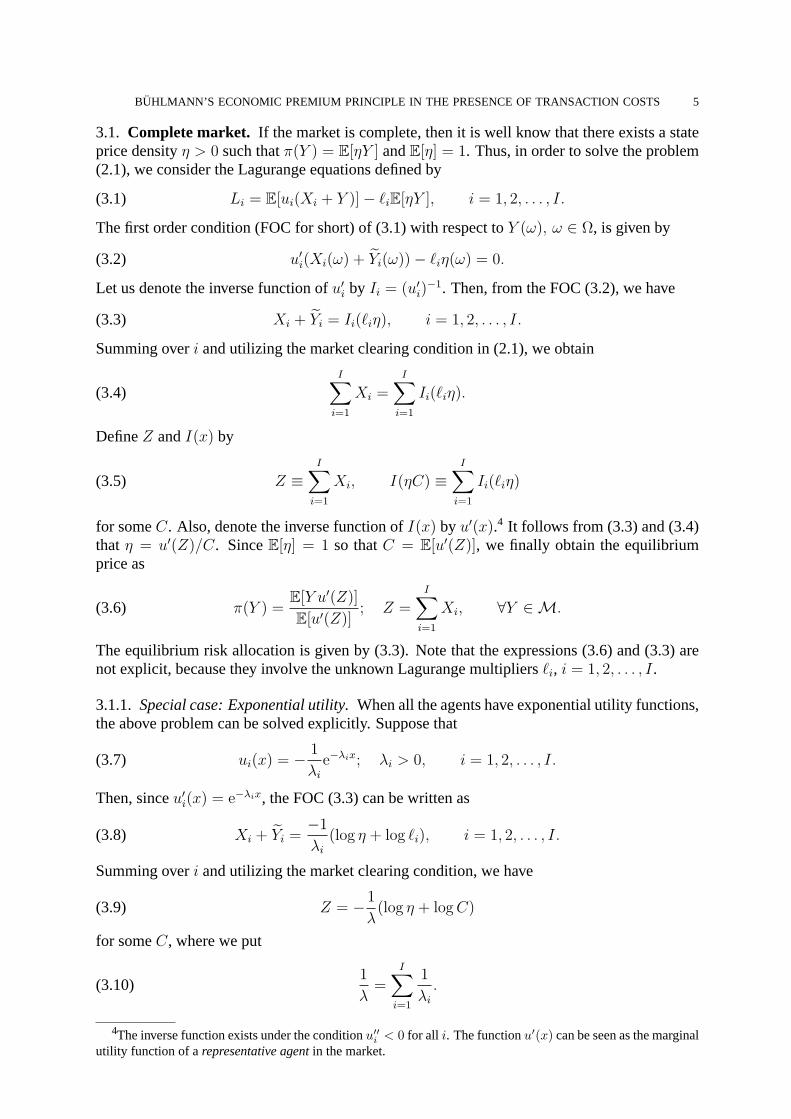
3.1. Complete market. If the market is complete, then it is well know that there exists a stateprice densityη > 0 such thatπ(Y ) = E[ηY ] andE[η] = 1. Thus, in order to solve the problem(2.1), we consider the Lagurange equations defined by
(3.1) Li = E[ui(Xi + Y )]− ℓiE[ηY ], i = 1, 2, . . . , I.
The first order condition (FOC for short) of (3.1) with respect toY (ω), ω ∈ Ω, is given by
(3.2) u′i(Xi(ω) + Yi(ω))− ℓiη(ω) = 0.
Let us denote the inverse function ofu′i by Ii = (u′
i)−1. Then, from the FOC (3.2), we have
(3.3) Xi + Yi = Ii(ℓiη), i = 1, 2, . . . , I.
Summing overi and utilizing the market clearing condition in (2.1), we obtain
(3.4)I∑
i=1
Xi =I∑
i=1
Ii(ℓiη).
DefineZ andI(x) by
(3.5) Z ≡I∑
i=1
Xi, I(ηC) ≡I∑
i=1
Ii(ℓiη)
for someC. Also, denote the inverse function ofI(x) by u′(x).4 It follows from (3.3) and (3.4)that η = u′(Z)/C. SinceE[η] = 1 so thatC = E[u′(Z)], we finally obtain the equilibriumprice as
(3.6) π(Y ) =E[Y u′(Z)]
E[u′(Z)]; Z =
I∑i=1
Xi, ∀Y ∈ M.
The equilibrium risk allocation is given by (3.3). Note that the expressions (3.6) and (3.3) arenot explicit, because they involve the unknown Lagurange multipliersℓi, i = 1, 2, . . . , I.
3.1.1. Special case: Exponential utility.When all the agents have exponential utility functions,the above problem can be solved explicitly. Suppose that
(3.7) ui(x) = − 1
λi
e−λix; λi > 0, i = 1, 2, . . . , I.
Then, sinceu′i(x) = e−λix, the FOC (3.3) can be written as
(3.8) Xi + Yi =−1
λi
(log η + log ℓi), i = 1, 2, . . . , I.
Summing overi and utilizing the market clearing condition, we have
(3.9) Z = −1
λ(log η + logC)
for someC, where we put
(3.10)1
λ=
I∑i=1
1
λi
.
4The inverse function exists under the conditionu′′i < 0 for all i. The functionu′(x) can be seen as the marginal
utility function of arepresentative agentin the market.
6 MASAAKI KIJIMA AND AKIHISA TAMURA
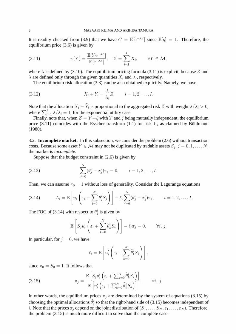
It is readily checked from (3.9) that we haveC = E[e−λZ ] sinceE[η] = 1. Therefore, theequilibrium price (3.6) is given by
(3.11) π(Y ) =E[Y e−λZ ]
E[e−λZ ]; Z =
I∑i=1
Xi, ∀Y ∈ M,
whereλ is defined by (3.10). The equilibrium pricing formula (3.11) is explicit, becauseZ andλ are defined only through the given quantitiesXi andλi, respectively.
The equilibrium risk allocation (3.3) can be also obtained explicitly. Namely, we have
(3.12) Xi + Yi =λ
λi
Z, i = 1, 2, . . . , I.
Note that the allocationXi + Yi is proportional to the aggregated riskZ with weightλ/λi > 0,where
∑Ii=1 λ/λi = 1, for the exponential utility case.
Finally, note that, whenZ = Y +ξ with Y andξ being mutually independent, the equilibriumprice (3.11) coincides with the Esscher transform (1.1) for riskY , as claimed by Buhlmann(1980).
3.2. Incomplete market. In this subsection, we consider the problem (2.6) without transactioncosts. Because some assetY ∈ M may not be duplicated by tradable assetsSj, j = 0, 1, . . . , N ,the market isincomplete.
Suppose that the budget constraint in (2.6) is given by
(3.13)N∑j=0
(θij − xij)πj = 0, i = 1, 2, . . . , I.
Then, we can assumeπ0 = 1 without loss of generality. Consider the Lagurange equations
(3.14) Li = E
[ui
(εi +
N∑j=0
θijSj
)]− ℓi
N∑j=0
(θij − xij)πj, i = 1, 2, . . . , I.
The FOC of (3.14) with respect toθij is given by
E
[Sju
′i
(εi +
N∑k=0
θikSk
)]− ℓiπj = 0, ∀i, j.
In particular, forj = 0, we have
ℓi = E
[u′i
(εi +
N∑k=0
θikSk
)],
sinceπ0 = S0 = 1. It follows that
(3.15) πj =E[Sju
′i
(εi +
∑Nk=0 θ
ikSk
)]E[u′i
(εi +
∑Nk=0 θ
ikSk
)] , ∀i, j.
In other words, the equilibrium pricesπj are determined by the system of equations (3.15) bychoosing the optimal allocationsθij so that the right-hand side of (3.15) becomes independent ofi. Note that the pricesπj depend on the joint distribution of(S1, . . . , SN , ε1, . . . , εN). Therefore,the problem (3.15) is much more difficult to solve than the complete case.

BUHLMANN’S ECONOMIC PREMIUM PRINCIPLE IN THE PRESENCE OF TRANSACTION COSTS 7
3.2.1. Special case: Exponential utility.Suppose that all the agents have exponential utilities(3.7). Then, from (3.15), we derive the following system of simultaneous equations:
(3.16) πj =E[Sje
−λi(εi+∑N
k=1 θikSk)
]E[e−λi(εi+
∑Nk=1 θ
ikSk)
] , ∀i, j > 0.
Note that the constant termλiθi0S0 is canceled out on both numerator and denominator. This
system of equations hasIN + N = N(I + 1) unknowns (i.e.,θij andπj) andIN equations in(3.16). Together with the market clearing condition, we haveIN + N = N(I + 1) equations.Hence, we can solve the simultaneous equation (3.16), although the solution may not be unique.Since the constant termλiθ
i0S0 does not matter in (3.16), the budget constraint is adjusted byθi0
so as to satisfy (3.13). The equilibrium risk exchanges are determined byyij = θij − xij.
In order to solve the problem, define the moment generating functions (MGFs)
mi(θ1, θ2, . . . , θN) = E[e−λi(εi+
∑Nj=1 θjSj)
], i = 1, 2, . . . , I,
for which the MGFsmi exist.5 The equilibrium pricesπj and the solutionsθij are determinedby the following simultaneous equations:
πj =∂
∂θjlogmi(θ
i1, θ
i2, . . . , θ
iN), ∀i, j > 0.
If in particular there are no residual risksεi, then we can solve the problem explicitly. Namely,let
(3.17) m(ρ1, ρ2, . . . , ρN) = E[e−
∑Nj=1 ρjSj
], i = 1, 2, . . . , I,
and consider the system of simultaneous equations
(3.18) πj = − ∂
∂ρjlogm(ρi1, ρ
i2, . . . , ρ
iN), ∀i, j > 0,
where we putρij = λiθij.
But, since the MGFm does not depend oni, the solutionsρij = λi(xij + yij) are also indepen-
dent ofi. That is, we haveλi(xij + yij) = ρj for someρj. It follows that
xij + yij =
ρjλi
, ∀i, j > 0,
and the market clearing condition together with (2.4) implies that
Aj =∑i
xij =
ρjλ;
1
λ=∑i
1
λi
, ∀i, j > 0.
Therefore, we obtainρj = λAj so that(xij+ yij)Sj =
λλiAjSj. Hence, the equilibrium allocation
is given by
(3.19) Xi + Yi =N∑j=1
(xij + yij
)Sj =
λ
λi
Z; Z =N∑j=1
AjSj, i = 1, 2, . . . , I.
The equilibrium prices are then expressed from (3.16) as
(3.20) πj =E[Sje
−λZ ]
E[e−λZ ]; Z =
N∑j=1
AjSj, j = 1, 2, . . . N,
5We need to assume that the MGFs exist in order for the equilibrium prices to exist in the exponential utilitycase. Note that this excludes the log-normally distributed assets.
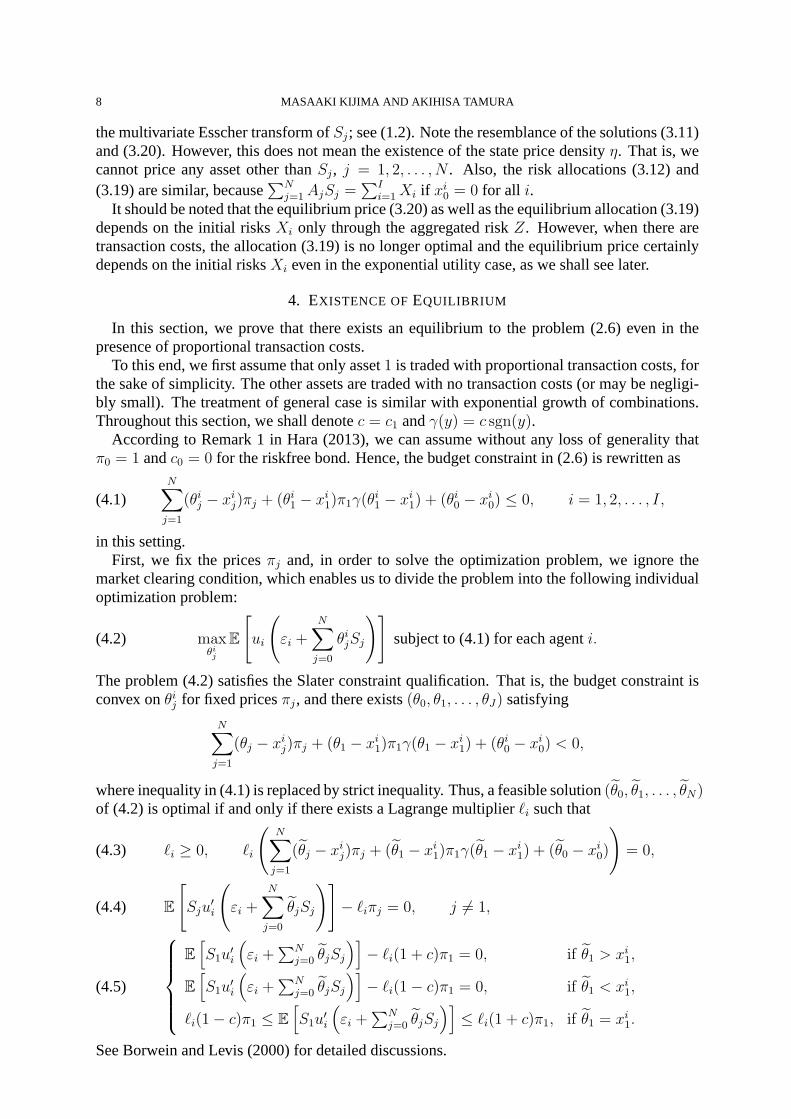
8 MASAAKI KIJIMA AND AKIHISA TAMURA
the multivariate Esscher transform ofSj; see (1.2). Note the resemblance of the solutions (3.11)and (3.20). However, this does not mean the existence of the state price densityη. That is, wecannot price any asset other thanSj, j = 1, 2, . . . , N . Also, the risk allocations (3.12) and(3.19) are similar, because
∑Nj=1AjSj =
∑Ii=1Xi if xi
0 = 0 for all i.It should be noted that the equilibrium price (3.20) as well as the equilibrium allocation (3.19)
depends on the initial risksXi only through the aggregated riskZ. However, when there aretransaction costs, the allocation (3.19) is no longer optimal and the equilibrium price certainlydepends on the initial risksXi even in the exponential utility case, as we shall see later.
4. EXISTENCE OFEQUILIBRIUM
In this section, we prove that there exists an equilibrium to the problem (2.6) even in thepresence of proportional transaction costs.
To this end, we first assume that only asset1 is traded with proportional transaction costs, forthe sake of simplicity. The other assets are traded with no transaction costs (or may be negligi-bly small). The treatment of general case is similar with exponential growth of combinations.Throughout this section, we shall denotec = c1 andγ(y) = c sgn(y).
According to Remark 1 in Hara (2013), we can assume without any loss of generality thatπ0 = 1 andc0 = 0 for the riskfree bond. Hence, the budget constraint in (2.6) is rewritten as
(4.1)N∑j=1
(θij − xij)πj + (θi1 − xi
1)π1γ(θi1 − xi
1) + (θi0 − xi0) ≤ 0, i = 1, 2, . . . , I,
in this setting.First, we fix the pricesπj and, in order to solve the optimization problem, we ignore the
market clearing condition, which enables us to divide the problem into the following individualoptimization problem:
(4.2) maxθij
E
[ui
(εi +
N∑j=0
θijSj
)]subject to (4.1) for each agenti.
The problem (4.2) satisfies the Slater constraint qualification. That is, the budget constraint isconvex onθij for fixed pricesπj, and there exists(θ0, θ1, . . . , θJ) satisfying
N∑j=1
(θj − xij)πj + (θ1 − xi
1)π1γ(θ1 − xi1) + (θi0 − xi
0) < 0,
where inequality in (4.1) is replaced by strict inequality. Thus, a feasible solution(θ0, θ1, . . . , θN)of (4.2) is optimal if and only if there exists a Lagrange multiplierℓi such that
ℓi ≥ 0, ℓi
(N∑j=1
(θj − xij)πj + (θ1 − xi
1)π1γ(θ1 − xi1) + (θ0 − xi
0)
)= 0,(4.3)
E
[Sju
′i
(εi +
N∑j=0
θjSj
)]− ℓiπj = 0, j = 1,(4.4)
E[S1u
′i
(εi +
∑Nj=0 θjSj
)]− ℓi(1 + c)π1 = 0, if θ1 > xi
1,
E[S1u
′i
(εi +
∑Nj=0 θjSj
)]− ℓi(1− c)π1 = 0, if θ1 < xi
1,
ℓi(1− c)π1 ≤ E[S1u
′i
(εi +
∑Nj=0 θjSj
)]≤ ℓi(1 + c)π1, if θ1 = xi
1.
(4.5)
See Borwein and Levis (2000) for detailed discussions.
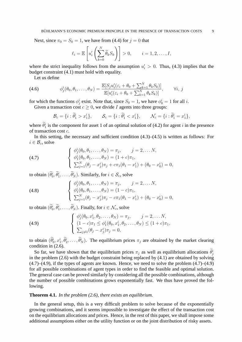
BUHLMANN’S ECONOMIC PREMIUM PRINCIPLE IN THE PRESENCE OF TRANSACTION COSTS 9
Next, sinceπ0 = S0 = 1, we have from (4.4) forj = 0 that
ℓi = E
[u′i
(N∑k=0
θkSk
)]> 0, i = 1, 2, . . . , I,
where the strict inequality follows from the assumptionu′i > 0. Thus, (4.3) implies that the
budget constraint (4.1) must hold with equality.Let us define
(4.6) ϕij(θ0, θ1, . . . , θN) =
E[Sju′i(εi + θ0 +
∑Nk=1 θkSk)]
E[u′i(εi + θ0 +
∑Nk=1 θkSk)]
, ∀i, j
for which the functionsϕij exist. Note that, sinceS0 = 1, we haveϕi
0 = 1 for all i.Given a transaction costc ≥ 0, we divideI agents into three groups:
Bc = i : θi1 > xi1, Sc = i : θi1 < xi
1, Nc = i : θi1 = xi1,
whereθi1 is the component for asset 1 of an optimal solution of (4.2) for agenti in the presenceof transaction costc.
In this setting, the necessary and sufficient condition (4.3)–(4.5) is written as follows: Fori ∈ Bc, solve
(4.7)
ϕij(θ0, θ1, . . . , θN) = πj, j = 2, . . . N,
ϕi1(θ0, θ1, . . . , θN) = (1 + c)π1,∑Nj=1(θj − xi
j)πj + cπ1(θ1 − xi1) + (θ0 − xi
0) = 0,
to obtain(θi0, θi1, . . . , θ
iN). Similarly, for i ∈ Sc, solve
(4.8)
ϕij(θ0, θ1, . . . , θN) = πj, j = 2, . . . N,
ϕi1(θ0, θ1, . . . , θN) = (1− c)π1,∑Nj=1(θj − xi
j)πj − cπ1(θ1 − xi1) + (θ0 − xi
0) = 0,
to obtain(θi0, θi1, . . . , θ
iN). Finally, for i ∈ Nc, solve
(4.9)
ϕij(θ0, x
i1, θ2, . . . , θN) = πj, j = 2, . . . N,
(1− c)π1 ≤ ϕi1(θ0, x
i1, θ2, . . . , θN) ≤ (1 + c)π1,∑
j =1(θj − xij)πj = 0,
to obtain(θi0, xi1, θ
i2, . . . , θ
iN). The equilibrium pricesπj are obtained by the market clearing
condition in (2.6).So far, we have shown that the equilibrium pricesπj as well as equilibrium allocationsθij
in the problem (2.6) with the budget constraint being replaced by (4.1) are obtained by solving(4.7)–(4.9), if the types of agents are known. Hence, we need to solve the problem (4.7)–(4.9)for all possible combinations of agent types in order to find the feasible and optimal solution.The general case can be proved similarly by considering all the possible combinations, althoughthe number of possible combinations grows exponentially fast. We thus have proved the fol-lowing.
Theorem 4.1. In the problem (2.6), there exists an equilibrium.
In the general setup, this is a very difficult problem to solve because of the exponentiallygrowing combinations, and it seems impossible to investigate the effect of the transaction coston the equilibrium allocations and prices. Hence, in the rest of this paper, we shall impose someadditional assumptions either on the utility function or on the joint distribution of risky assets.
10 MASAAKI KIJIMA AND AKIHISA TAMURA
4.1. Exponential Utilities. As in Subsection 3.2.1, suppose thatεi = 0 andu′i(x) = e−λix for
all i. In this case, the functionϕij defined in (4.6) is given by
(4.10) ϕij(θ1, . . . , θN) =
E[Sje−λiP ]
E[e−λiP ], P =
N∑j=1
θjSj.
Letρij = λiθj, as before, and denote the MGF (moment generating function) of(S1, S2, . . . , SN)by (3.17), i.e.,
m(ρ1, ρ2, . . . , ρN) = E[e−
∑Nj=1 ρjSj
]for which the MGF exists. It is easy to verify that
ϕij(θ0, θ1, . . . , θN) = − ∂
∂ρjlogm(ρi1, . . . , ρ
iN).
Hence, it is enough to define the function
ϕj(ρ1, ρ2, . . . , ρN) = − ∂
∂ρjlogm(ρ1, ρ2, . . . , ρN),
which makes the exponential case simpler.Now, the problem (4.7)–(4.9) is reduced to the following: Fori ∈ Bc, solve
(4.11)
ϕj(ρ1, ρ2, . . . , ρN) = πj, j = 2, . . . N,
ϕ1(ρ1, ρ2, . . . , ρN) = (1 + c)π1.
The solution is denoted byρ+j (c), j = 1, 2, . . . , N . Similarly, for i ∈ Sc, solve
(4.12)
ϕj(ρ1, ρ2, . . . , ρN) = πj, j = 2, . . . N,
ϕ1(ρ1, ρ2, . . . , ρN) = (1− c)π1.
The solution is denoted byρ−j (c), j = 1, 2, . . . , N . Finally, for i ∈ Nc, solve
(4.13)
ϕj(λix
i1, ρ2, . . . , ρN) = πj, j = 2, . . . , N,
(1− c)π1 ≤ ϕ1(λixi1, ρ2, . . . , ρN) ≤ (1 + c)π1.
The solution is denoted byρ0ij (c), j = 2, . . . , N , which may be dependent oni. In either cases,ρ0 is obtained by the budget constraint.
Given these solutions, the equilibrium allocation of agenti is obtained as follows: For asset1, we have
θi1 =
ρ+1 (c)/λi, i ∈ Bc,
ρ−1 (c)/λi, i ∈ Sc,
xi1, i ∈ Nc.
Summing overi, the market clearing condition is obtained as
(4.14) A1 = ρ+1 (c)∑i∈Bc
1
λi
+ ρ−1 (c)∑i∈Sc
1
λi
+∑i∈Nc
xi1.
Similarly, for the other assetj, j ≥ 2, we have
θij =
ρ+j (c)/λi, i ∈ Bc,
ρ−j (c)/λi, i ∈ Sc,
ρ0ij (c)/λi, i ∈ Nc.
Summing overi, the market clearing condition is obtained as
(4.15) Aj = ρ+j (c)∑i∈Bc
1
λi
+ ρ−j (c)∑i∈Sc
1
λi
+∑i∈Nc
ρ0ij (c)
λi
, j ≥ 2.
BUHLMANN’S ECONOMIC PREMIUM PRINCIPLE IN THE PRESENCE OF TRANSACTION COSTS 11
Note that we have3N + N0(N − 1) unknowns (ρ+j (c), ρ−j (c) andπj for j ≥ 1, andρ0ij (c) for
i ∈ Nc andj ≥ 2) and the same number of equations (N in (4.11) and (4.12),N0(N − 1)in (4.13), andN in total in (4.14) and (4.15) together), whereN0 = |Nc| denotes the numberof agents in the classNc. Hence, in principle, we can solve the simultaneous equations, if thedivision of agents were known.
The allocationsθi0 are determined by the budget constraint as follows. Fori ∈ Bc, we have
(4.16) θi0 = xi0 −
N∑j=1
(ρ+j (c)
λi
− xij
)πj − cπ1
(ρ+1 (c)
λi
− xi1
).
Similarly, for i ∈ Sc,
(4.17) θi0 = xi0 −
N∑j=1
(ρ−j (c)
λi
− xij
)πj + cπ1
(ρ−1 (c)
λi
− xi1
),
and fori ∈ Nc,
(4.18) θi0 = xi0 −
N∑j=2
(ρ0ij (c)
λi
− xij
)πj.
From (4.16)–(4.18) together with (4.14) and (4.15), we obtain the market clearing condition forasset0 as
I∑i=1
θi0 = A0 − 2cπ1
∑i∈Bc
(ρ+1 (c)
λi
− xi1
)≤ A0,
which means that the riskfree asset may be left in the market.6
Example 4.1.Suppose that the transaction costc is sufficiently large, so that no agents want totrade asset 1, i.e.,Bc = Sc = ∅. In this case, the problem (4.13) is only relevant, and we haveθij = ρ0ij (1)/λi, i = 1, 2, . . . , I, for every assetj. Recall that, in general, the quantityρ0ij (1)depends oni. The equilibrium price is given from (4.10) as
(4.19) πj =E[Sje
−λZi ]
E[e−λZi ], Zi =
1
λ
(λix
i1S1 +
N∑j=2
ρ0ij (1)Sj
); j ≥ 2,
for all i, where the market clearing condition is given by
Aj =I∑
i=1
ρ0ij (1)
λi
, j ≥ 2.
Note that the prices in (4.19) are affected by the non-traded asset1. WhenS1 is independent ofthe other assets, it is readily shown that the prices are given by (3.20) withA1 = 0.
4.2. Risks Are Normally Distributed. Next, we consider the case that(S1, S2, . . . , SN) isnormally distributed. In this subsection, we assume that0 ≤ c ≤ 1. The mean vector andcovariance matrix are denoted byµ = (µj) andΣ = (σij), respectively. It is readily obtainedthat
logm(ρ1, . . . , ρN) = −N∑j=1
ρjµj +1
2
∑j,k
σjkρjρk.
6This does not cause any problem, since the riskfree bond is traded with no transaction costs and does notcontribute to the functionϕj for the exponential case.
12 MASAAKI KIJIMA AND AKIHISA TAMURA
Thus, we have
(4.20) ϕj(ρ1, . . . , ρN) = µj −N∑k=1
σjkρk.
For the convenience of description, we use the vectorsπ = (πj), a = (Aj) andρi = (ρij),and divide the covariance matrixΣ as
Σ =
(σ11 σ⊤
σ Σ
), σ =
σ21...
σN1
, Σ =
σ22 · · · σ2N...
.. ....
σN2 · · · σNN
,
whereσ⊤ denotes the transpose ofσ. For anN -dimensional vectorz = (z1, z2, . . . , zN)⊤, we
denote the(N − 1)-dimensional vector(z2, . . . , zN)⊤ by z. For example,π = (π2, . . . , πN)⊤
for π.From (4.20), the equations forj = 2, . . . , N of (4.11)−(4.13) are written in matrix form as
µ− ρi1σ − Σρi = π, i = 1, 2, . . . , I,
whereρi1 = λixi1 if i ∈ Nc. SinceΣ is positive definite (i.e., nonsingular), we have
(4.21) ρi = Σ−1 (
µ− ρi1σ − π), i = 1, 2, . . . , I.
The market clearing conditions (4.14) and (4.15) are rewritten as
(4.22) A1 =I∑
i=1
ρi1λi
and
(4.23) a =I∑
i=1
1
λi
ρi = Σ−1
(1
λµ− σ
I∑i=1
ρi1λi
− 1
λπ
),
respectively, where1λ=∑I
i=11λi
as in (3.10). It follows from (4.22) and (4.23) that
(4.24) π = µ− λ(A1σ + Σa
).
Hence, when risks are normally distributed, the pricesπj, j ≥ 2, are not affected from thetransaction costc of asset1. Moreover, the pricesπj, j ≥ 2, are given as the multivariate Esschertransform (3.20). To see this, we need the following lemma. See Kijima and Muromachi (2001)for the proof.
Lemma 4.1. Suppose that(X,Z) is normally distributed. Then,
E[f(X)e−λZ ] = E[f(X − λcov(X,Z))]E[e−λZ ]
for anyf(x) for which the expectations exist, wherecovdenotes the covariance operator.
Theorem 4.2. When risks are normally distributed, the pricesπj, j ≥ 2, are given by themultivariate Esscher transform
πj =E[Sje
−λZ ]
E[e−λZ ]; Z =
N∑k=1
AkSk, j ≥ 2,
that are independent of the transaction costc of asset1.
BUHLMANN’S ECONOMIC PREMIUM PRINCIPLE IN THE PRESENCE OF TRANSACTION COSTS 13
Proof. From (4.24), we have
πj = µj − λN∑k=1
σjkAk, j = 2, 3, . . . , N,
which is just the multivariate Esscher transform (3.20) from Lemma 4.1. In contrast, the equilibrium allocation depends on the cost, as we show next. From (4.21) and
(4.24),ρi can be represented as a function ofρi1 and given by
(4.25) ρi(ρi1) = λ(A1Σ
−1σ + a
)− ρi1Σ
−1σ.
Under the condition (4.25),ϕ1(ρi) is also a function ofρi1 and given by
ϕ1(ρi1, ρ
i(ρi1)) = µ1 −B − ρi1r,
where we define
B = λ(A1σ
⊤Σ−1σ + σ⊤a
), r = σ11 − σ⊤Σ
−1σ.
Here, note that, sincer > 0,
Σ−1 =
1r
−1r
(Σ
−1σ)⊤
−1r
(Σ
−1σ)
Σ−1
+ 1r
(Σ
−1σ)(
Σ−1σ)⊤
must be positive definite.
Recalling thatρij = λi(xij + yij), we define
vi(y) = si − λiry, si = µ1 −B − λirxi1,
for eachi = 1, . . . , I. In order to find equilibrium prices and equilibrium allocations, it isenough to determiney11, y
21, . . . , y
I1 andπ1 satisfying
(4.26)
vi(y
i1) = (1 + c)π1, yi1 > 0,
vi(yi1) = (1− c)π1, yi1 < 0,
(1− c)π1 ≤ si ≤ (1 + c)π1, yi1 = 0,
under the market clearing condition for asset1, i.e.,
(4.27)I∑
i=1
yi1 = 0.
Condition (4.26) can be reformulated as
(4.28) yi1 =
(si − (1 + c)π1)/rλi, si > (1 + c)π1,
(si − (1− c)π1)/rλi, si < (1− c)π1,
0, otherwise,
and the partition(Bc,Sc,Nc) of agents is rewritten asBc = i : si > (1 + c)π1,Sc = i : si < (1− c)π1,Nc = i : (1− c)π1 ≤ si ≤ (1 + c)π1.
From (4.28), equation (4.27) is restated as
(4.29)∑i∈Bc
1
λi
(si − (1 + c)π1) +∑i∈Sc
1
λi
(si − (1− c)π1) = 0.

14 MASAAKI KIJIMA AND AKIHISA TAMURA
We first consider the casec = 0. From (4.28), we have
yi1 =si − π1
λir, i = 1, . . . , I.
This together with (4.27) implies
π1
λ=
I∑i=1
π1
λi
=I∑
i=1
siλi
=µ1 −B
λ− rA1.
Hence, we obtain the equilibrium priceπ01 for c = 0 as
π01 = µ1 −B − λrA1 = µ1 − λ
(σ11A1 + σ⊤a
),
which is given by the multivariate Esscher transform by the proof of Theorem 4.2.We assume thatπ0
1 > 0 in the sequel. We will show that i) an equilibrium priceπc1 for
c ∈ [0, 1] exists and it is uniquely determined by (4.29) ifBc,Sc = ∅, ii) πc1 > 0, and iii)
the buying price(1 + c)πc1 is increasing inc and the selling price(1 − c)πc
1 is decreasing inc.Then, from (4.28), the trading volumes|yi1| are decreasing as the costc gets large and, from thedefinition ofBc andSc, once some agent stops trading, he/she will never return for trading.
Suppose thatc with πc1 > 0 (e.g.,c = 0) is given. Ify11 = y21 = · · · = yI1 = 0 for thec, then,
for all c′ ∈ [c, 1], πc′1 = πc
1 satisfies (4.26) and (4.27), and the results i), ii) and iii) hold. Hence,we assume that
(4.30) there existsyi1 = 0 for c.
Equation (4.29) implies thatπc1 is uniquely determined by
(4.31) πc1 =
∑i∈Bc∪Sc
siλi
1λB
+ 1λS
+ c(
1λB
− 1λS
) , 1
λB
=∑i∈Bc
1
λi
,1
λS
=∑i∈Sc
1
λi
.
We note that (4.29) and (4.30) guarantee the existence ofλB andλS, and thatc ∈ [0, 1] together
with λB, λS > 0 also guarantees1λB
+ 1λS
+ c(
1λB
− 1λS
)= 0. In a range includingc for which
Bc andSc are unchanged,πc1 is a continuous function ofc, and hence,(1 + c)πc
1 and(1− c)πc1
are also continuous functions ofc.For simplicity, we assume that(1 − c)πc
1 < si < (1 + c)πc1 for all i ∈ Nc. In this case,
conversely, we can slightly changec preserving the partition(Bc,Sc,Nc). Now, we slightlyincreasec to c′. Then, (4.29) forc′ andπc′
1 holds for the sameBc andSc. That is,
(4.32)1
λB
(1 + c)πc1 +
1
λS
(1− c)πc1 =
1
λB
(1 + c′)πc′
1 +1
λS
(1− c′)πc′
1 =∑
i∈Bc∪Sc
siλi
.
Suppose to the contrary that(1 + c)πc1 ≥ (1 + c′)πc′
1 , which impliesπc1 > πc′
1 , becausec < c′
andπc1 > 0. From (4.32), we have0 ≤ (1 − c)πc
1 ≤ (1 − c′)πc′1 . This is, however, impossible
because(1− c) > (1− c′) ≥ 0 andπc1 > πc′
1 . Hence, we obtain(1 + c)πc1 < (1 + c′)πc′
1 , whichimplies that(1− c)πc
1 > (1− c′)πc′1 andπc′
1 > 0.If there isi ∈ Nc such that(1 − c)πc
1 = si or si = (1 + c)πc1, then we can show the same
results by redefining the partition(Bc,Sc,Nc) byBc = i : si ≥ (1 + c)πc
1,Sc = i : si ≤ (1− c)πc
1,Nc = i : (1− c)πc
1 < si < (1 + c)πc1.
By repeating the same argument and modifying the partition(Bc,Sc,Nc) until c = 1 or (4.30)is violated, we can show i), ii) and iii), as desired. We thus have the following results.
BUHLMANN’S ECONOMIC PREMIUM PRINCIPLE IN THE PRESENCE OF TRANSACTION COSTS 15
Theorem 4.3.Suppose that all the risky assets are normally distributed. Then, for any costc ∈[0, 1], an equilibrium priceπc
1 of asset1 exists, and is a unique solution of(4.29)if Bc,Sc = ∅.The equilibrium allocation isxi
1+yi1, whereyi1 is given by(4.28), for asset1 andxij+yij = ρij/λi,
whereρij are given by(4.25), for assetj, j ≥ 2.
The next seemingly plausible results have been proved in Hara (2013) for the single risky-asset case with general distribution.
Corollary 4.1. When all the risks are normally distributed, the buying price(1 + c)πc1 is in-
creasing inc, the selling price(1 − c)πc1 is decreasing inc, and the trading volumes|yi1| are
decreasing inc in equilibrium. Once some agent stops trading, he/she will never return fortrading.
5. THE EQUILIBRIUM WHEN TRANSACTION COSTS AREVERY SMALL
Suppose that the transaction costscj are so small that all the assets in the market are tradedby all the agents, i.e.,yij = 0 or θij − xi
j = 0. Then, as in the case of no transaction costs, wecan define the Lagurange equations
Li = E
[ui
(εi +
N∑j=0
θijSj
)]− ℓi
N∑j=0
(θij − xij)πj(1 + cjsgn(θ
ij − xi
j))
for all i = 1, 2, . . . , I, and the FOC with respect toθij is given by
(5.1) E
[Sju
′i
(εi +
N∑k=0
θikSk
)]− ℓiπj(1 + cjsgn(θ
ij − xi
j)) = 0, ∀i, j.
This is possible, because we assume thatθij − xij = 0 and the sign functionsgn(y) is differen-
tiable excepty = 0.
5.1. CARA-Normal Case. In this subsection, we consider exponential utilities, i.e.,u′i(x) =
e−λix, i = 1, 2, . . . , I. Then, from (5.1), we derive the following system of simultaneous equa-tions:
(5.2) E[Sje
−λi(εi+∑N
k=1 θikSk)
]= πj(1 + cjsgn(θ
ij − xi
j))E[e−λi(εi+
∑Nk=1 θ
ikSk)
], ∀i, j,
because as beforeℓi = E[e−λi(εi+∑N
k=1 θikSk)]. Recall thatsgn(y) = 1 if y > 0 andsgn(y) = −1
if y < 0.In the following, we assume that the pricesπj are strictly positive and denote
Rj =Sj − πj
πj
, j = 1, 2, . . . , N ; Riε =
εi − πi(εi)
πi(εi), i = 1, 2, . . . , I,
whereπi(εi) represents the (unobservable) pricing functional ofεi. In this section, we assumethat the random vector(R1, . . . , RN , R
ε1, . . . , R
εI) defined above is normally distributed.
Following the ordinary arguments, we obtain
εi +N∑j=1
θijSj =N∑j=1
πj θijRj + πi(εi)R
εi + πi(εi) +
N∑j=1
θijπj.
It follows that the FOC (5.2) can be written as
(5.3) E[(1 +Rj)e
−λiΓi]= (1 + cjsgn(y
ij))E
[e−λiΓ
i], ∀i, j,
16 MASAAKI KIJIMA AND AKIHISA TAMURA
where
(5.4) Γi ≡N∑j=1
πj(xij + yij)Rj + πi(εi)R
εi ,
becauseθij = xij + yij. A direct application of Lemma 4.1 to (5.3) yields
µj − λicov(Rj,Γi) = cjsgn(y
ij), yij = 0,
whereµj = E[Rj] denotes the mean rate of return of assetj. It follows from the definition (5.4)of Γi that
(5.5)1
λi
(µj − cjsgn(yij)) = πi(εi)σ
εij +
N∑k=1
πk(xik + yik)σkj, ∀i, j,
whereσεij = cov(Rj, R
iε) andσij = cov(Ri, Rj).
Because we have assumed that the equilibrium exchangesyij are all nonzero, Equation (5.5)holds for all i andj. Summing overi in (5.5) and utilizing the market clearing condition in(2.6), we obtain
(5.6)1
λ(µj − cjΓj(yj)) = ξj +
N∑k=1
πkAkσkj, j = 1, 2, . . . , N,
whereξj =∑
i πi(εi)σεij, λ is given in (3.10), andΓj(yj) is defined by
(5.7) Γj(yj) =I∑
i=1
λ
λi
sgn(yij), j = 1, 2, . . . , N,
with yj = (y1j , y2j , . . . , y
Ij ). The quantitycjΓj(yj) is interpreted as the weighted sum of the
(signed) trading costs of assetj in equilibrium. Note that, since−1 ≤ sgn(y) ≤ 1, we obtain
(5.8) −1 < Γj(yj) < 1, j = 1, 2, . . . , N,
for anyyj. The inequalities in (5.8) are strict, because the market clearing condition cannothold otherwise.
Whenyij are all nonzero, equations in (5.6) can be written in matrix form as
1
λ(µ− Γ)− ξ = Σ diag(Aj)π,
whereµ = (µj), Γ = (cjΓj(yj)), ξ = (ξj) andπ = (πj) areN -dimensional vectors, whereΣ = (σij) is anN ×N symmetric matrix, and wherediag(Aj) denotes the diagonal matrix oforderN with diagonal elementsAj. Assuming that the covariance matrixΣ is positive definite(hence, it is invertible), the above equation is solved as
(5.9) π =1
λdiag(A−1
j )Σ−1(µ− λξ), µ = µ− Γ,
whereµ = (µj), µj = µj − cjΓj(yj), denotes the vector ofcost-adjustedmean rates of returnin equilibrium. Hence, the equilibrium prices are written formally as
(5.10) πj =1
λAj
Σ−1j (µ− λξ), j = 1, 2, . . . , N,
whereΣ−1j denotes thejth row vector of the inverse matrixΣ−1.
BUHLMANN’S ECONOMIC PREMIUM PRINCIPLE IN THE PRESENCE OF TRANSACTION COSTS 17
In the following, we denote the equilibrium price without transaction costs (i.e.,cj = 0 forall j) by πNT
j for assetj. In this setting, it is readily proved that, even in the presence of residualrisksεi, the equilibrium prices are given by
(5.11) πNTj =
1
λAj
Σ−1j (µ− λξ) =
E[Sje−λZ ]
E[e−λZ ], j = 1, 2, . . . , N,
the multivariate Esscher transform ofSj, where
(5.12) Z =I∑
i=1
Xi =N∑j=1
AjSj +I∑
i=1
εi
stands for the aggregated risk.Note that, in the presence of transaction costs, while the mean rates of return are adjusted,
the covariance matrix is unchanged. Hence, comparing (5.10) with (5.11), we conclude thefollowing.
Theorem 5.1.Suppose that the transaction costscj are so small that the optimal exchangesyijare all nonzero. Then, the equilibrium price of assetj in the presence of transaction costs isgiven by the multivariate Esscher transform ofSj, i.e.,
(5.13) πj =E[Sje
−λZ ]
E[e−λZ ], Z =
N∑j=1
AjSj +I∑
i=1
εi,
whereSj denotes the asset price with the cost-adjusted mean rate of return,µj = µj−cjΓj(yj).
Note that (5.10) can be written alternatively as
πj =1
λAj
Σ−1j (µ− λξ)− 1
λAj
Σ−1j Γ = πNT
j − 1
λAj
Σ−1j Γ, j = 1, 2, . . . , N.
Here, the quantitiesΓj(yj) can be positive or negative, depending on the optimal risk exchangesyij, which are assumed to be nonzero in Theorem 5.1. Hence, the equilibrium prices in thepresence of transaction costs can be higher or lower than those without transaction costs.
Next, the equations in (5.5) can be written in matrix form as
1
λi
(µ− γi)− ξi = Σ diag(xij + yij)π,
whereγi = (cjsgn(yij)) andξi = (πi(εi)σ
εij) areN -dimensional vectors. Substitution of the
equilibrium price (5.9) into the above equation yields
1
λi
Σ−1(µ− γi − λiξi) = diag(xi
j + yij)1
λdiag(A−1
j )Σ−1(µ− Γ− λξ).
It follows that the equilibrium allocation is formally given as
(5.14) (xij + yij)Sj =
λ
λi
AjSj
Σ−1j (µ− γi − λiξ
i)
Σ−1j (µ− Γ− λξ)
, j = 1, 2, . . . , N.
Recall from (3.19) that the partλλiAjSj corresponds to the equilibrium allocation when there
are no transaction costs and residual risks.
18 MASAAKI KIJIMA AND AKIHISA TAMURA
5.2. Pricing of derivative securities. Suppose that there are derivative securities (written onsome traded assets) in the market and that the equilibrium pricing formula (5.13) is valid. In thissubsection, we show that the risk-neutral pricing method holds true for the pricing of derivativesecurities under some conditions.
Consider, as an example, a call optionY with strike priceK written on assetSj. That is, wedenote the payoff by
Y = (Sj −K)+ = f(Rj), f(x) = (πj(1 + x)−K)+,
where(x)+ = maxx, 0 andRj = (Sj−πj)/πj. According to the equilibrium pricing formula(5.13), the price of the call option is given by
(5.15) π(Y ) =E[Y e−λZ ]
E[e−λZ ],
whereY denotes thecost-adjustedpayoff of the call option.Suppose thatY = f(Rj) and, instead of (5.15), the call option price is given by
(5.16) π(Y ) =E[f(Rj)e
−λZ ]
E[e−λZ ],
whereRj denotes the cost-adjusted rate of return ofSj. Note that the transaction costs totrade derivative securities are usually negligible, because agents must pay the option premiums.However, since the transaction costs of other assets affect the option price in equilibrium, theformulaY = f(Rj) is merely an assumption in our framework. This assumption states that thetransaction costs of other assets do not affect the price of the derivative.
Suppose further that there are so many assets traded in the market, and so the aggregated riskZ can be approximated by a normally distributed random variable.7 Since thecost-adjustedrateof returnRj is normally distributed by our early assumption, i.e.,
Rj = µj + σjwj,
wherewj denotes a standard normal variate, it then follows from (5.16) and Lemma 4.1 that
(5.17) π(Y ) = E [f(µj + σjwj − λcov(Rj, Z))] .
However, in this setting, the price ofSj must be given by
πj = E [πj(1 + µj + σjwj − λcov(Rj, Z))] ;
hence, we haveµj = λcov(Rj, Z). It follows that the call option price is given by
(5.18) π(Y ) = E [(πj(1 + σjwj)−K)+] .
This is so, because the risk premiumλcov(Rj, RZ) in (5.16) is already reflected in the priceπj
of the underlying assetSj in equilibrium. This result is important for practice, because we donot need to estimate the unknown (unobservable) parametersλ andcov(Rj, RZ) for the pricingof derivative securities, provided that the above assumptions hold.
Now, recall thatex ≈ 1 + x for x small in the magnitude. Hence, if the volatilityσj is smallenough, the following approximation is justified:
(5.19) 1 + σjwj ≈ eσjwj−σ2j /2,
where the termσ2j/2 is subtracted to have the same mean in both sides. In this case, from (5.18),
we haveπ(Y ) = E[(πje
σjwj−σ2j /2 −K)+].
7See Wang (2003) for the justification of this assumption.
BUHLMANN’S ECONOMIC PREMIUM PRINCIPLE IN THE PRESENCE OF TRANSACTION COSTS 19
Finally, it is readily shown that the call option price is given by
π(Y ) = πjΦ(d)−KΦ(d− σj), d =log(πj/K)
σj
+σj
2,
the famous Black–Scholes formula (1973) withrf = 0 andT = 1.
6. COCLUDING REMARKS
In this paper, we examine the Buhlmann’s equilibrium pricing model (1980) in the presenceof proportional transaction cost. It is shown that an equilibrium exists under some mild con-ditions and the multivariate Esscher transform (1.2) is an appropriate probability transform forthe pricing of insurance risks even in the market with transaction costs.
In the simplest case that only asset 1 is traded with transaction cost (the other assets aretraded with no transaction costs), we derive an explicit form of equations to be solved for theequilibrium. In particular, for the CARA-normal case, it is shown that an equilibrium priceπc
1
of asset1 with transaction costc is a unique solution of a linear equation (4.29) and the pricesof the other assets are given by the multivariate Esscher transform. In this case, as the costcincreases, the buying price(1+ c)πc
1 is increasing, the selling price(1− c)πc1 is decreasing, and
the trading volumes|yi1| are decreasing in equilibrium.When the transaction costs are so small, we show that the equilibrium asset prices are given
by the multivariate Esscher transform for the CARA-normal case. In this case, while the meanrates of return of the assets are adjusted by the transaction costs, the volatilities of the assets arenot affected by them in equilibrium.
When there is a derivative security in the market, we show that the risk-neutral pricing methodis possible under the assumption that the transaction costs of other assets do not affect the priceof the derivative. However, in our framework, the transaction costs of other assetsdo affectthe option price in equilibrium and, hence, the risk-neutral method may not be applicable in thepresence of transaction costs. It is of great interest to investigate this problem within the generalequilibrium framework as a future research.
REFERENCES
[1] Aase, K. (1993), “Equilibrium in a reinsurance syndicate: Existence, uniqueness and characterization,”AstinBulletin, 23, 185–211.
[2] Aase, K. (2002), “Equilibrium pricing in the presence of cumulative dividends following a diffusion,”Math-ematical Finance, 12, 173–198.
[3] Black, F. and M. Scholes (1973), “The pricing of options and corporate liabilities,”Journal of PoliticalEconomy, 81, 637–654.
[4] Borwein, J. M. and A.S. Levis (2000),Convex Analysis and Nonlinear Optimization, Theory and Examples,Springer-Verlag, New York.
[5] Buhlmann, H. (1980), “An economic premium principle,”Astin Bulletin, 11, 52–60.[6] Buss, A., R. Uppal and G. Vilkov (2011), “Asset prices in general equilibrium with transaction costs and
recursive utility,” Working Paper, Goethe University.[7] Hara, C. (2013), “Asset prices, trading volumes, and investor welfare in markets with transaction costs,”
Discussion Paper, No.862, Kyoto Institute of Economic Research, Kyoto University.[8] He, L. and Z. Liang (2009), “Optimal financing and dividend control of the insurance company with fixed
and proportional transaction costs,”Insurance: Mathematics and Economics, 44, 88–94.[9] Højgaard, B. and M. Taksar (1998), “Optimal proportional reinsurance policies for diffusion models with
transaction costs,”Insurance: Mathematics and Economics, 22, 41–51.[10] Kabanov, Y. and M. Safarian (2009),Markets with Transaction Costs: Mathematical Theory, Springer-
Verlag, Berlin.[11] Kijima, M. (2006), “A multivariate extension of equilibrium pricing transforms: The multivariate Esscher
and Wang transforms for pricing financial and insurance risks,”ASTIN Bulletin, 36, 269–283.[12] Kijima, M. and Y. Muromachi (2001), “Pricing of equity swaps in a stochastic interest rate economy,”Journal
of Derivatives, 8, 19–35.
20 MASAAKI KIJIMA AND AKIHISA TAMURA
[13] Kijima, M. and Y. Muromachi (2008), “An extension of the Wang transform derived from Buhlmann’s eco-nomic premium principle for insurance risk,”Insurance: Mathematics and Economics, 42, 887–896.
[14] Malamud, S., E. Trubowitz, and M.V. Wuthrich (2008), “Market consistent pricing of insurance products,”Astin Bulletin, 38, 483–526.
[15] Tsanakas, A. and N. Christofides (2006), “Risk exchange with distorted probabilities,”Astin Bulletin, 36,219–243.
[16] Wang, S.S. (2002), “A universal framework for pricing financial and insurance risks,”Astin Bulletin, 32,213–234.
[17] Wang, S.S. (2003), “Equilibrium pricing transforms: New results using Buhlmann’s 1980 economic model,”Astin Bulletin, 33, 57–73.