Sec. 8.6 CSTR with Heat Effects

I EsornpIe 8-9 CSTR wilh o Cooling Coil

A cooling coil has been located in equipment storage for use in the hydration of propylene oxide discussed in Example 84. The cooling coil has 40 ft2 of cooling surface and the cooling water flow rate inside the coil is sufficiently l q e that a con- stant coolant temperature of 85°F can be maintained. A typical overall heat-transfer coefficient for such a coil is 100 Btu/h-ft2."E W111 the seactor satisfy the previous constraint of 125°F maximum temperature if the cooling coil is used?

SnEutidn

If u7e assume that the conling coil rakes up negligible reactor volume, the conver- sion calculated as a function of temperature from the mole balance is the same as that in Example 8-8 [Equation (EB-8.10)].

1. Combining the mole baiance, stoichiornetry, and rate law, we hav,=. from Example 8-8.

'Zhe reactor cannot be used becai~se ~t

uoiH exceed the specified maximum

temperature of 585%.

~k - (2 084 X 10") n p (- 16,3061 T) XWB = - - I + t k 1 + (2.084 X 1 O J 2 ) exp (- 16.306) T )

T ('RI

Figure E8-8.2 Tbe conversions XEa and Xw, as a function of temperature.

(E8-8,

2. Energy halance. Neglecting the work hy the stirrer, we combine Quations I

(5-27) and (8-50) to write

LTA( To - T ) - I((AHORr(TR) + ACptT- TH)) = SO,Cp,[T- T,) (Eg-9.1)

F A "

T i s in "R.

532 Steady-State Nonisothermal Reactor Design Cht

Energy Balance

We can now use the glass lined reactor

Uvlng Example Problerr

SoEcin~ Ae enerxy balance for X,, yields

The cooling coil term in Equation (E8-9.2) is

Ud - Btu - - ( IW -) (40 ft2) - - 92.9 Btu (E8- F~~ h + ft?."F (43.03 lb moIl'h) lb mold "F

Recall that the cooling temperahre is

T, = 8S°F = 545"R

The numerical values of all other terns of Equation (E8-9.2) are identic: those given in Equation (E8-8.12) but with the addition of the heat excha tern.

We now have two equations [(ES-8.80) and (E8-9,411 and two unknowns. X and The POLYMA~I program and solution to these two Equations (EB-8.10), X

and (E8-9.4). XEa. are given in Tables ES-9.1 and E8-9.2. The exiting tempera and conversion are 103.7"F (563.7"R) and 36.46, respectively. i.e..

I T = 5 6 4 " ~ and x = 0.361

Equations:

Nonlmear quationr

[ I I rrX) = X-(M3.3'(T*5.5uH92.9'fl-MS))I(~7'(T-528)1 = 0

I21 IrTI 5 X-~au*W< I+uuXI = 0

Explicit equatmns

Ill 1x11 =0.1?29 i2l A = I6.WlWlZ

131 E = 32m

I41 R = 1 . a7

Sobrion outpur to Polymath program in Table E8-9.1 is shown in Tahk E8-9.

TABW E8-9.2. EWLE 8-8 CSTR WH HEAT EXCHANGE

Variablt Valuc f l X ) Ini Guesr

X 0 3636087

7 563.73893

2.U3E-1 I 0.367

-5.4118-10 5W

lau 0.1229

A 1.696Ecl3

E 3 . U W

R 1.987

k 4.WF.9843

Sec. 8.7 Multiple Steady States 533

8.7 MutZiple Steady States

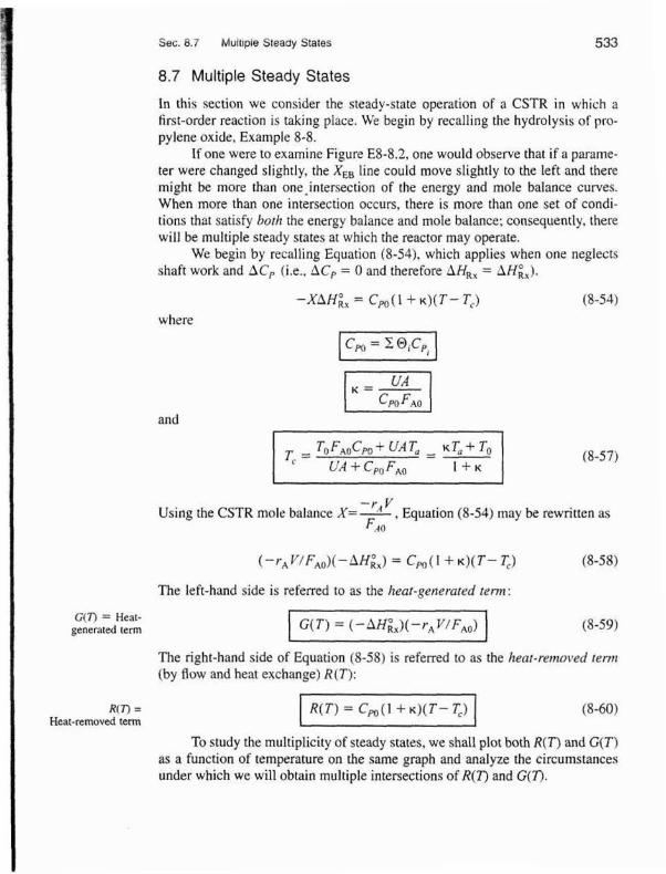
In this section we consider the steady-state operation of a CSTR in which a first-order reaction is taking place. We begin by recalling the hydrolysis of pro- pylene oxide, Example 8-8.

If one were to examine Figure €8-8.2, one would observe that if a parame- ter were changed slightly, the X,, line could move slightly ta the left and there might be more than one-intersection of the energy and mote balance curves. W e n more than one intersection occurs, there is more than one set of condi- tions that satisfy both the energy balance and moEe balance: consequently, there will be multiple steady states at which the reactor may operate.

We begin by recalling Equation (8-54), which applies when one neglects shaft work and LC, (i.e.. AC, = 0 and therefore AH,, = AH:,).

- X A N i , = C,(1+ K)(T- T,) (8-54) where

and

- r Y Using the CSTR mole balance X= -, Equation (8-54) may be rewritten as

F.4 0

The left-hand side is referred to u the heat-generated term: I I

C(7) = Heat- generated term

The right-hand side of Equation (8-58) i s referred to as the heat-removed term (by flow and heat exchange) R(T>:

R(p = Heat-removed term

(8-60)

To study the multiplicity of steady states. we shall pIot both R(T) and G(T) as a function of temperarue on the same graph and analyze the circurnstance.w under which we will obtain multiple intersections of R(T) and G ( 0 .

534 Steady-State Nonisothermal Reactor Design Chap. 8

8.7.1 Heat-Removed Term, f l T )

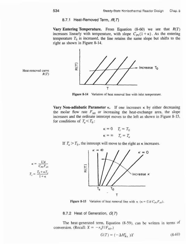
Vary Entering Temperature. From Equation (8-60) we see that RIT) increases linearly with temperature, with slope C,(1 + K) . As the entering temperature To Is increased. the line retains the same slope but shifts to the right as shown in Figure 8-14.

Heat-removed curve R(T)

Figure 8-14 Variation of heat removai line with inlet temperature.

Vary Non-adiabatic Parameter K. If one increases K by either decreasing the molar flow rate FA, or increasing the heat-exchange area. the slope increases and the ordinate intercept moves to the left as shown in Figure 8-15, for conditions of T, < To :

If T, > To, the intercept will move to the right as K increases.

Figure 8-15 Varialion of hear removal line with K (K = Url!C,F,,).

0.7.2 Heat of Generation, G( f )

The heat-generated term, Equation 18-59], can be written in terms of conversion. (Recall: X = - r,VI FA,.)

G ( T ) = {-AH",, )X (8-61 )

Sec. 8.7 Multiple Steady States 535

To obtain a plot of heat generated, CCT), as a function of temperaturr-, we must solve for X as a function of T using the f3TFt mole balance, the sate law, and stoichiometry. For example, for a first-order liquid-phase reaction, the CSTR mole balance becomes

FA&- VOCAOX v= -- kc* kcA,(] - X )

Solving for X yields

I st-order reaction rk x= - I + zk

Substituting for X in Quation (8-61), we obtain

Finally, substituting for k in terms of the Amhenius equation, we obtain

Note that equations analogous to Equation (8-63) for G ( T ) c3n be derived for other reaction orders and for reversible reactions simply by solving the CSTR mole balance for X . For example, for the second-order liquid-phase reaction

the corresponding heat generated is

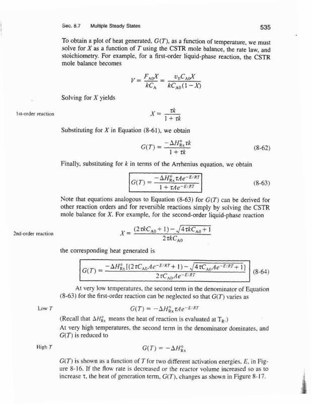
At very low temperatures, the second term in the denominator of Equation (8-63) for the first-order reaction can be neglected so that G(T) varies as

LOW T G ( T ) = -AHi,zAe-E'Rr

(Recall that AH,", means the heat of reaction is evaluated at T,.) At very high temperatures. the second term in the denominator dominates. and G(T) is reduced to

G(T) is shown as a function of Tfor two different activation energies, E, in Fig- ure 8-16. If Ehe flow rate 1s decrea\ed or the reactor volume increased so as to increase 7, the heat of generation term, G(T), chan~es as shown i n Figure 8-17.

536 Steady-State Nonisothermal Reactor Design Chal

High E

- S s

Figure 8-16 Heat generation curve. Figure 8-17 Variation of heat generatton curve with space-time

Heat-generated curves. G(Tj

8.7.3 Ignition-Extinction Curve

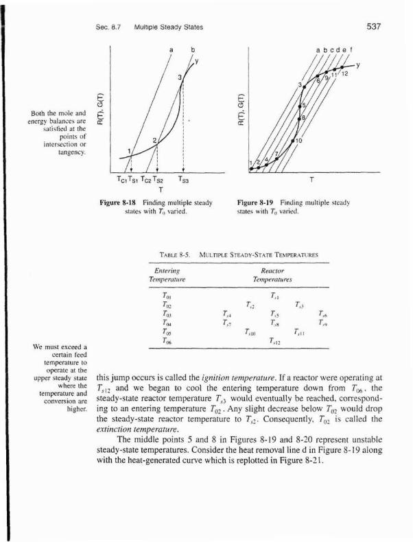
The points of intersection of R(T) and GtT) give us the temperaturn which the reactor can operate at steady state. Suppose that we begin to feed reactor at some relatively low temperature. To, . If we construct our G(T) i R ( T ) curves, illustrated by curves y and a, respectiveIy. in Figure 8-18, we that there will be only one point of intersection, point 1. From this point of in section. one can find the steady-state temperature in the reactor, T,, , by follc ing a vertical line down to the T-axis and reding off the temperature as show! Figure 8- 18.

If one were now to increase the entering temperature to T,. the G curve, y, would remain unchanged, but the R(Tf curve would move to the ri) as shown by Iine b i n Figure 8- t 8, and will now intersect the G(T) at point 2 : be tangent at point 3. Consequently, we see from Figure 8-1 8 that there are 1 steady-state temperatures. T,, and T,, , that can be reaIized in the CSTR for entering temperature TO:. If the entering temperature is increased to ir;,, R(T) curve, line c (Figure 8-19). intersects the G(T) three times and there three steady-state temperatures. As we continue to increase To, we finally re line e, in which there are only two steady-state temperatures. By further incrt ing T, we reach line f, corresponding no T, , in which we have only one tern1 ature that will satisfy both the mole and energy balances. For the six enter temperatures, we can Form Table 8-5, relating the entering temperature to possible reactor operating temperatures. By plotting T, as a function of T,, , obtain the well-known ignition-extinction cune shown in Figure 8-20. FE this figure we see that as the entering temperature is increased. the steady-s temperature increases along the bottom line until To, is reached. Any fnct io~ a degree increase in temperature beyond Tm and the steady-state reactor tern1 ature will jump up to T,,, , as shown in Figure 8-20. The temperature at wk

Sec. 8.7 Multrpfe Steady States 537

+-. + 5

Both the mole and A

energy bnlnnccs are mtidicd at the

points of intsncction or

tangency.

We must exceed a certain feed

temprilture to operate at the

upper ~ teady state where the

temperature and conversion are

higher.

Figure I(-I8 F~nding multiple steady Figure 8-19 Finding ~nulriple steady ~tatek with T,, varred ~ t a t e ~ w ~ t h T, vaned.

this jump occurs is called the ignition temperature. If a reactor were operating at T,,, and we began to cool the entering temperature down from To,, the sredy-state reactor temperature T,, wouId eventually be reached. correspond- ing to an entering temperature To,. Any slight decrease below To? would drop the steady-state reactor temperature to TF3. Consequently, To? is called the e.~tincfian temperarure.

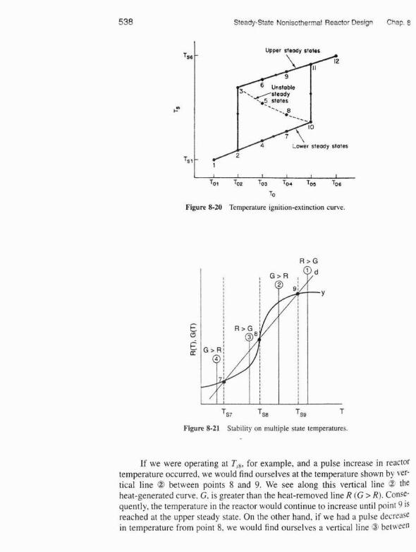
The middle points 5 and 8 in Figures 8-19 and 8-20 represent unstabIe steady-state temperatures. Consider the heat removal line d in Figure 5- 19 along with the heat-generated curve which is replotted in Figure 8-21.

Steady-State Nonisotherrnal Reactor Desigl Chap. 8

Figure 8-20 Temperature ignition-extinction curve.

T ~ 7 T& T~ T

Figure 8-21 Stab~litj on multiple state temperatures

If we were operating at TsB! for example, and a pulse increase in reactor temperature occurred. we would find ourselves at the temperature shown by ver- tical Iine CZ) be~ween points 8 and 9. We see along this vertical line @ the heat-generated curve. G. is greater than the heat-removed line R (G > R). Conse- quently. the temperature in the reactor would continue to increase until p n t 9 i s reached at the upper cteady state. On the other hand. if we had a pulse decrease in temperature from point 8. we would find ourselves a vertical line ~3 helween

Sec. 8.7 Multiple Steady States 539

points 7 and 8. Here we see the heat-removed curve is greater than the heat-gen- erated curve so the temperature will continue to decrease until the lower aeady state is reached. That js a srnajl change in temperature either above or below the middle steady-state temperature, T,, will cause the reactor temperature to move away from this middle steady state. Steady states that behave in the manner are said to be unstable.

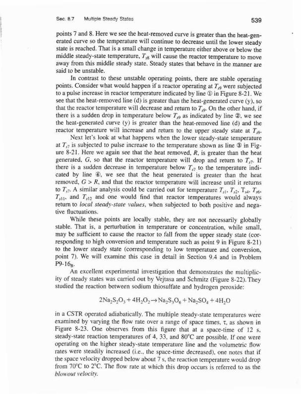
In contrast to these unstable operating points, there are stable operating points. Consider what would happen if a reactor operating at T, were subjected to a pulse increase in reactor temperature indicated by Iine O in Figure 8-2 1. We see that the heat-removed line (d) is greater than the heat-generated curve (y), so that the reactor temperature will decrease and return to T* On the other hand, if there is a sudden drop in temperature below T* as indicated by line a, we see the heat-generated curre {y) is greater than the, heat-removed line (d) and the reactor temperatue will increase and return to the upper steady slate at T&.

Next let's look at what happens when the lower steady-state temperature at T,, is subjected to pulse increase to the ternperature shown as line 3 in Fig- ure 8-21. Here we again see that the heat removed, R, is greater than the heat generated, G. so that the reactor temperature will drop and return to Ts7. If there is a sudden decrease in temperature below T,, to the temperature indi- cated by Iine @, we see that the heat genesated is greater than the heat removed, G > R, and that the reactor temperature will increase until i t returns to T,,. A similar analysis could be carried out for ternperature TS1, T,?. T,,, Ts6, T,,,, and T,,, and one would find that reactor temperatures would always return to local sleadv-srare values, when subjected to both positive and nega- tive fluctuations.

While these points are locally stable, they are not necessarily globally stable. That is, a perturbation in temperature or concentration. while srnaIl, may be sufficient to cause the reactor to fall from the upper steady state (cor- responding to high conversion and temperature such as point 9 in Figure 8-21) to the lower steady state (corresponding to low temperature and conversion, point 7) . We will examine this case in detail in Section 9.4 and in Problem P9-16B.

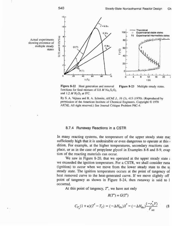
An excellent experimental investigation that demonsrrates the muItiplic- ity of steady states was camed out by Vejtasa and Schmitz (Figure 8-22).They studied the reaction between sodium thiosulfate and hydrogen peroxide:

in a CSTR oprated adiabatically. The multiple steady-state temperatures were examined by varying the Row rate over a range of space times, r, as shown in Figure 8-23. One observes from this figure that at a space-time of 12 s, steady-state reaction temperatures of 4, 33, and 80°C are possible. If one were operating on the higher steady-state temperature line and rhe volwmetric flow rates were steadily increased (i.e., the space-time decreased). one notes that if the space velocity dropped below about 7 s. the reaction temperature would drop from 70°C to Z°C. The flow rate at which this drop occurs is referred to as the ~ I O M ' O U ~ velocin'.

540 Steady-State Nonisothermal Reactor Design Ch

Figure 8-22 Heat generation and removal Figure 8-23 Multiple steady states. functions for feed mixture of 0.8 M NalSIO, and 1.2 M H,Ot at PC.

100

By S. A. Vejtasa and R. A. Schmitz. AlChE J. , 16 (3). JIS (1970). (Reproduced by permission uf the American Inst~tute of Chemical Engineers. Copyright Q 1970 AIChE. All right reserved.) See Journal Critique Problem PSC-4.

- f h@oreticul - o Expenmental stabk SMtes - P + Expenmental ~nterrwdare states

8.7.4 Runaway Reactions in a CSTR

0" Y, - I-

1 I I I I I I # t I 0 X) 40 60 80 0 [I 4 B 1 2 1 6 M :

rl'cl f ( 5 )

In many reacting systems, the temperature of the upper steady state ma! sufficiently high that it is undesirable or even dangerous to operate at this I

dition. For example, at the higher temperatures, secondary reactions can place, or as in the case of propylene glycol in Examples 8-8 and 8-9, evap tion of the reacting materials can mcur.

We saw in Figure 8-20, that we operated at the upper steady state i

we exceeded the ignition temperature. For a CSTR, we shall consider tuna (ignition) to wcur when we move from the lower steady sbte to the ul steady state. The ignition temperature occurs at the point of tangency of heal removed curve to the heat-generated curve. If we move slightly off point of tangency as shown in Figure 8-24, then runaway is said to t occurred.

At this point of tangency, T, we have not only

Sec. 8.7 Multiple Szeady States

Tc T* T

Flgure 8-24 Runaway in a CSTR.

but also the slopes of the R(7) and G(T) curves are also equal. For the heat-removed curve. the slope i s

and for the heat-generated curve, the slope is

Assuming that the reaction is irreversibIe and follows a power law model and that the concentrations of the reacting s p i e s are weak functions of temperature.

- r ~ = (Aem', fn(Ci) 18-68]

then

Substituting for the derivative of (-r,) wrt Tin Equation (8-67)

542 Steady-Stele Nonisotherrnal Reactor D ~ i g n Chap. 8

where

Equating Equations (8-66) and (8-69) yields

Next, we divide Equation (8-65) by Equation (8-70) so obtain the fellow- ing AT value for a CSTR operating at T = T:

I f t h i . ~ diflerence herween rhe reacfor temperazure and T,, AT,, is exceeded, transifion m the rrpper sready stare will occur. For many industrial reactions, UFT is typically between 16 and 24, and the reaction temperatures may be between 300 to 500 K. Consequently, this critical temperature difference AT, wiIl be somewhere around 15 to 30°C.

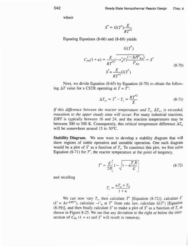
Stability Diagram. We now want to develop a stability diagram that will show regions of stable operation and unstable operation. One such diagram would be a pIot of S* as a function of T,. To construct this plot, we first solve Equation (8-71) for T. the reactor temperature at the point of tangency,

and recalling

We can now vary 7,. then caIcutate T [Equation ( 8 - J Z ) ] , calculate k" (k* = Ae-E/RT*), calculate -r*, at T from rate law. calculate G ( T ) [Equation (8-5411, and then finally calculate S* to make a plot of S* as a function of T, as shown in Figure 8-25. We see that any deviation to the right or below the inter- section of Cw ( 1 + K ) and S' will result in runaway.

Sec, 8.8 Nonisothermal Mdliple Chrnical Reactions

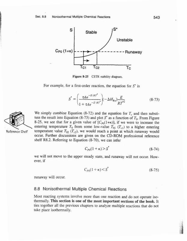
EYpre 8-25 CSTR stability diagram.

For example, for a first-order reaction, the equation for S is

We simply combine Equation (8-72) and the equation for T, and then substi- tute the resdt into Equation (8-73) and plot S* as a function of Tw From Figure 8-25, we see that for a given value of [C,(I+u)I, if we were to increase the entering temperature To from some Iow-value To',, (T,,) to a higher entering

Shelf temperature value Tm IT,,), we would reach a point at which runaway would occur. Further discussions are given on the CD-ROM professional reference shelf R8.2. Referring to Equation (8-701, we can infer

we will not move to the upper steady state, and runaway will not occur. How- ever, if

runaway will occur.

8.8 Nonisothermal Multiple Chemical Reactions

Most reacting systems involve more than one reaction and do not operate iso- thermally. This section is one of the most important sections of the book. It ties together all the previous chapters to analyze multiple reactions rhar do not take place isothermally.

544 Steady+State NonisolherrnaT Reactor Design CV

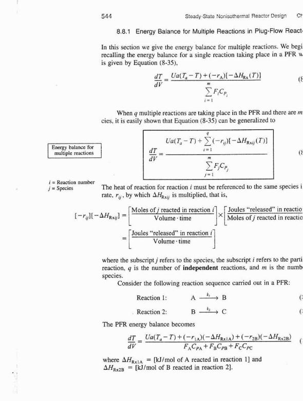
8.8.1 Energy Balance for Multiple Reactions in Plug-Flow Reacts

In this section we give the energy balance for multiple reactions. We begi recalling the energy balance for a single reaction taking place in a PFR H

is given by Equation (8-351,

When q multiple reactions are taking place in the PFX and there are m cies, ir is easily shown that Equation (8-35) can be generalized to

i = Reaction number j = Species The heat of reaction for reaction i must be referenced to the same species i

rate, r , , by which AHRxb is multiplied, that is,

Moles o f j reacted in reaction i Joules "released"' in reactio [-rqll[-AH~,l = Volume - time Moles of j reacted in reactic

= [,,,Ies ~'releasd" in reaction i Volume time I

where the subscript j refers 10 the species, the subscript d refers to the parti reaction, q is the number of independent reactions, and m is the numb species.

Consider the following reaction sequence cartied out in a PFR:

Reaction 1: A k' ) B (:

Reaction 2: B k l > C (:

The PIX energy balance becomes

where AHRxlA = FJlmol of A reacted in reaction 11 and AH,,, = [kllrnol of B reacted in reaction 21.

Living Example Jroblem

One of the major I

goais of this text is hat the reader will

be able ta solve multiple reactions with heat effects.

Sec. 8.8 Nonisothermal Multiple Chern~cal Reactions

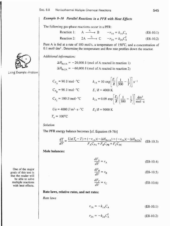
Example 8-18 ParalIeL Reoc~bns in a PFR with Heat EflecIs

1 The foilowing gas-phase reaciions occur i n r PFR:

Reaction 1: A & B - r , , = k,,C,, IE8- 10.1) k, Reaction 2: 2A C -r lA = kZ4?* (E8- 10.2)

Pure A i s fed at a rate of 100 molls. a ternprature of 150PC, and a concentration of 0. I rnolldm3 . Determine4 the temperature and Row rate profiles down the reactor.

AHR,,, = -20.000 J/(rnol of A reacted in reaction 1 )

AHR,?, = -60,000 J/(mol of A reacted in reaction 2)

Solslrion

The PFR energy balance becomes [cf. Equation (8-76)]

Mole balances:

Rate laws, relative rates, and net rates:

Rate Eaws

The algorithm for multiple reactions

w t h heat effects

546 Steady-State Nonisothermal Fleactor Oestgn Chap. 8

Reaction 1: 'IA = 5. - I , ~ I B = ~ ~ A C A - 1

Reaction 2:

Ner mtes:

Stoichiometry (gas phase AP = 0):

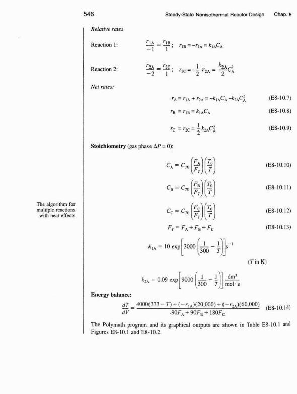
k , , = 10 exp 3000 - - - sL1 [ (3; :)I (Tin K)

k2* = 0.09 exp 9000 - - [ (3; h)] 2 Energy balance:

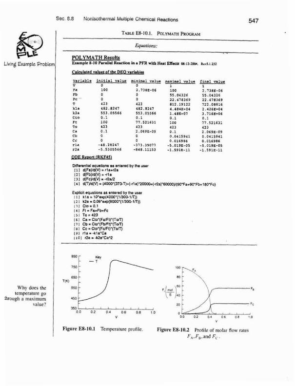
The Polymath program and its graphical outputs are shown in Table E8-10.1 and Figures E8-10.1 and E8-10.2.

Sec. 8.8 Nonisotherrnal Multipls Chemical Reactions 547

Lfving Eram~ic Problem I

TABLE E8- 10.1. POLYMAW PROGRAM

Equarim:

POLYMATH Results Examplt &-111 F*tnllcl R n a b In 4 PFR aILb Hm En=@ m-1Mwc. Ra3.1.u~

Splculrtd values or !C DEO mrlablra

Variablm initial value minim1 valua msximl vaf u t f L M ~ value v 0 0 1 1 Fd 100 9.7382-06 I00 2 .?>BE-06 m 0 0 35.04326 55.04326 FC - o D w.4-1a369 22.478369 T L a 3 423 812.19122 722.08816 kla 402.8247 482 .a247 4.4BPE+01 ?.4266+04 k21 5 5 3 . 0 5 5 6 6 551.05566 l.4BE*07 3.716I+O6 CTO 0.1 0.1 0.1 0.1 PC 100 77.521631 1 0 0 77.521631 TO 433 123 P O 3 423 Cb. 0.1 2 . 0 6 9 E - 0 9 0.1 2.069E-09 Cb 0 0 0.0415941 0 . 0 4 i 5 9 4 1 Cc 0 0 0 . 0 1 6 9 B 6 0.016986 ria -48.28947 -373 -39077 -5.019E-05 -5.019E-05 r21 -1.5305566 -840 .11153 - 1 . 5 9 1 E - 1 1 -1.591E-11

-rt lRKF451

I)IVWMIM B~U*IDM aa meted by me uaer 1 : I d(FaYd(W = r l u+Ra i 2 l dffbYdtW = -rla

f xpliil w & t M a as anrated by !he uner I I I k ~ a = ~ O ' ~ ~ ( * O W ' ( I / ~ [ K ~ . I ~ Q ) I 2 l k2e -O.OB'erp(QMXl'(l~9C&1rr)J 1 7 1 Cto = 0.1 1 4 I FI - Fa+Fb+Fe 151 To=423 161 Cs - Cto'(FaFl)'(Tdr) I? I Cb = Clo'{FWF!).(TdQ l a ] Cc - Cto'{FMt)'(TPrT) 191 r l a - -hla'Cn I 10 l Ra P -k2a'Cm

Why does the temperalure go

through a maximum va rue:'

850

550

4 M

0 0 0 2 0 4 06 0 8 1 0 V D O a 2 0 4 0 6 0 6 1 0

v

Figure E8-10.1 Temperature profile. Figure ES-10.2 Profile of molar flow rates F,.F,,and F,.

548 Steady-State Nonisothermal Reactor Design Cht

8.8.2 Energy Balance for Multiple Reactions in CSTR

RecalI that -F,,,X = r,V fur a CSTR and that AH,,(Ir) = AH;, + AC,(T - so that Equation (8-27) for the steady-state energy balance for a single reac may be written as

For g multiple reactions and m species, the CSTR energy balance becomes

Energy balance for multiple Substituting Equation (8-50) for Q, negIecting the work term. and assum

reactions in a constant heat capacities, Equation (8-80) becomes 1 CITR 1 For the two parallel reactions described in Example 8-10. the CSTR ene balance is

Mdor goal (8- of CRE One of the major goals of this text is to have the reader solve problems invc

ing multiple reactions with heat effects (cf. Problem P&-26c).

Example 8-11 Multiple Reactions in a CSTR

The elementary liquid-phase reactions

take place in a 10-dm3 CSTR. What are the effluent concentrations for a volume feed rate of 1000 drn31rnin at a concentration of A of 0.3 molldm3?

The inlet zernpture is 283 K.

Additional information:

k, = 3.3 min-I at 300 K. with E, = 9900 cat/rnol

k2 = 4.58 min-I at 500 K, with El = 27,000 callmol

Sec. 8.8 Nonisolherrnal Multiple Chemical Reactions 549

I hfi',,~, = -55.00fi Jlmol A UA = 40,000 JJrnin-K with r, = 57'C

I The &ons follow elcmentay rate laws

I. Mole Balance on Every Species A: Comb~ned mole balance and rate law for A:

Solving for C, g' ~ v e s US

I B: Combined mote balance and rate INI f a B:

I Solving for C, yields

1 2. Rate Laws:

I

3. Energy Balances: Applying Equation (8-82) to this system gives

Substituting for r l , and r13 and rearransing, we have

550 Steady-State Nonisothermal Reactor Design Chap. 8

Incrementing temperature in this manner is an easy

way to generale RU) and G(T) plots

Living Example Problen

When F = O G(T) = R(T) and the steady states

can be found.

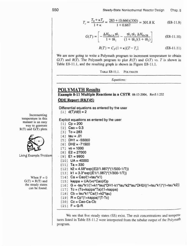
We are now going to write a Polymath program to increment temperature 10 obtain G(T) and R(r). The Polymath program to plot R ( T ) and G ( T ) vs. T i s shown in Table E8-11.1, and the resulting graph is shown in Figure E8-11.1.

POLYMATH Results Example 8-11 Multiple Reactions in a CS7"R 08-13-zW. Rev5.1.232

Differential equations as entered by the user [ 1 1 d(T)ld(t) = 2

Expl'iclt equations as entered by the user t l l Cp=200 [ a ] Cao=0.3 [ 3 J Toe283 [ 4 1 tau=.Ol [ 5 ] DHt =-55000 16 1 DH2 = -71 500 171 v0=1000 [ 8 ] €2 = 27000 191 El =9900 [10] VA=400M) t l l l Ta=330 [ 12 1 k2 = 4.58'exp((E2/1.987)*(1/500-7 m) 1 13 3 kl = 3.3*exp{(El/l.907)*(11300-1TT)) [ 14 1 Ca = Caol(1 +lau'kf ) [ 15 I kappa = UN(vo'Cao)lCp 11 6 1 G = -tau'kl/{l +kl * tau~~~1-k l ' t au+k2" tau*D~2~~( i+ t~u~k l ) * ( l+ t~u*k2~~ ( 17 I TC = (To+kappa'Ta)l( 1 +kappa) [ 18 I Cb = tau'kl'Cd(1 +k2r~u) [ 19 I R = Cp'f 1 +kappa)'(T-Tc) 120 I Cc = Cao-Ca-Cb [Ill F=G-R

We see that five steady states ( S S ) exist. The exit concenrrarions and tempem- tures listed in Table E8- 1 1.2 were interpre~ed from the labular output of the ~ o l ~ ~ n a t h program.