02/10/2012

1

www.bsc.es

Paris, October 2nd 2012

Jesús LabartaBSC

BSC Tools

2

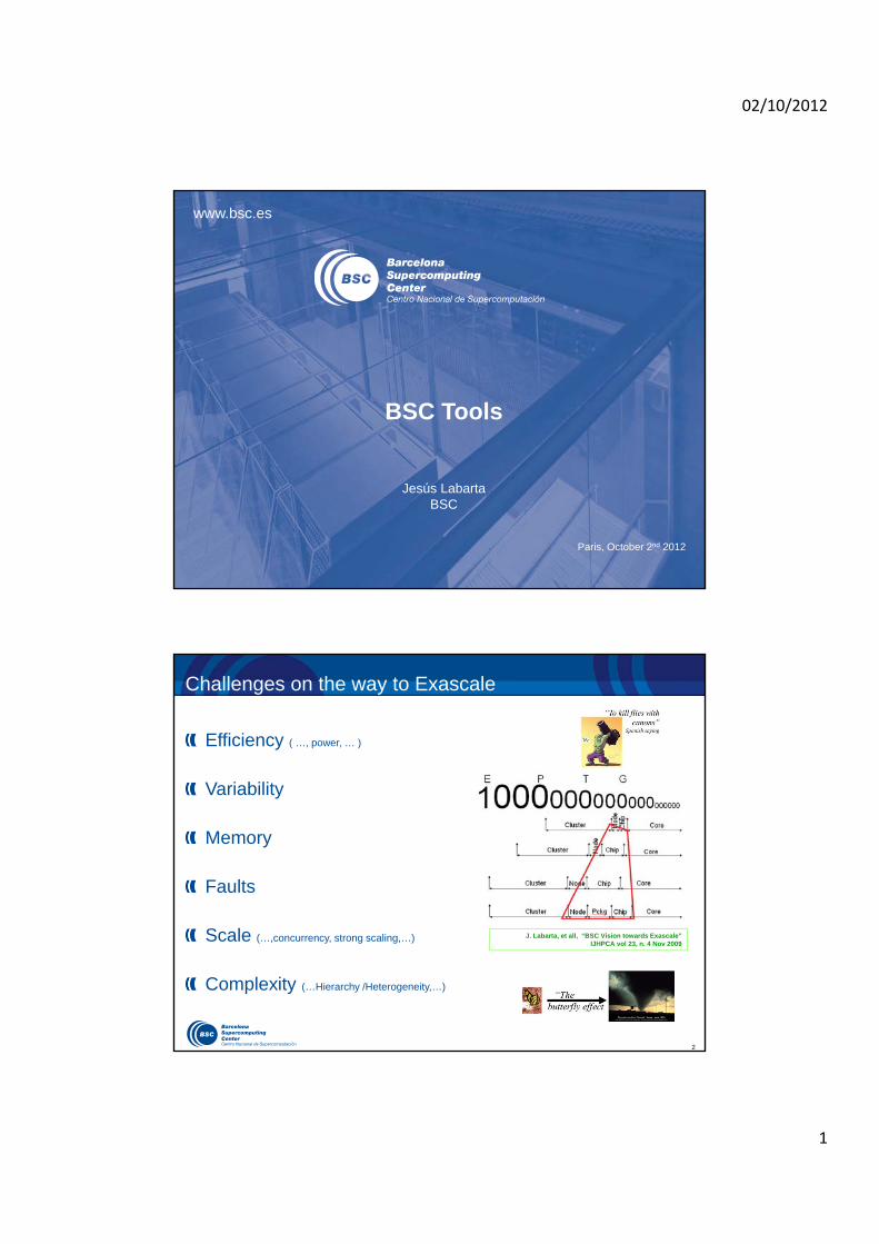
Challenges on the way to Exascale

Efficiency ( …, power, … )

Variability

Memory

Faults

Scale (…,concurrency, strong scaling,…)

Complexity (…Hierarchy /Heterogeneity,…)

J. Labarta, et all, “BSC Vision towards Exascale” IJHPCA vol 23, n. 4 Nov 2009

02/10/2012

2

3

Key issues

Programming model and run time– Language to express ideas– Runtime responsible for mapping them to resources– Smooth transition path, long lived efforts

Performance analysis tools– Avoid flying blind– The importance of details– How can we improve?– Need much more “Performance analytics”

Algorithms– Final target– A say in the solution

4

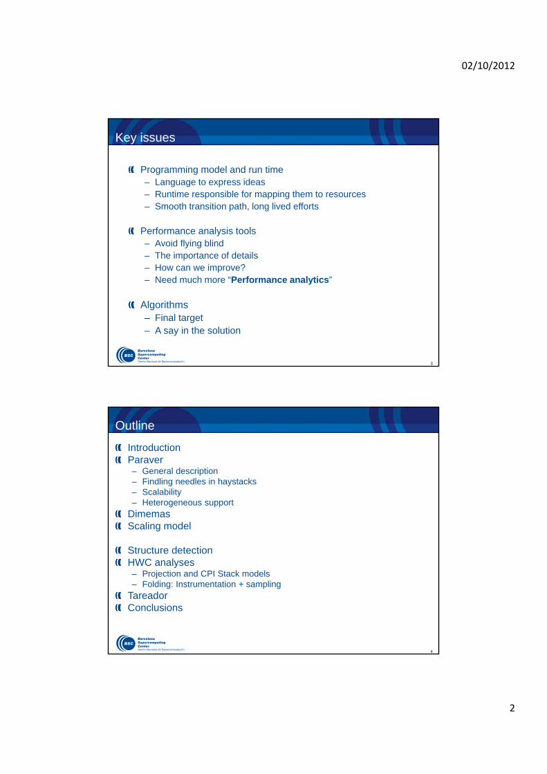
Outline

IntroductionParaver– General description– Findling needles in haystacks– Scalability– Heterogeneous support

DimemasScaling model

Structure detectionHWC analyses– Projection and CPI Stack models– Folding: Instrumentation + sampling

TareadorConclusions

02/10/2012

3

Performance Tools

6

Why Tools ?

Measurement techniques as enablers of science

Are becoming vital for program development at exascale– Fly with instruments: survive the unexpected, …– Not to shoot blind: Work in the right direction

Are important for “Lawyers”– Know who to blame

Are vital for system architects– Understand our systems, productivity

Performance analyst:– A specialist understanding displays

02/10/2012

4

Science

Advances linked to capability of observation and measurement

Tools in …

Computer Science

– printf()– timers

Performance analysis:

– A lot of speculation

• We see

• we talk about )(tf

b

adttf )(

8

Performance Analytics

Dominant practice– We focus a lot on capturing a lot of data

– but we present either everything or first order statistics

– and require new experiments without squeezing the potential information from the previous one

Need for performance analytics – Leveraging techniques from data analytics, mining, signal processing,

life sciences,…

– towards insight

– and models

02/10/2012

5

9

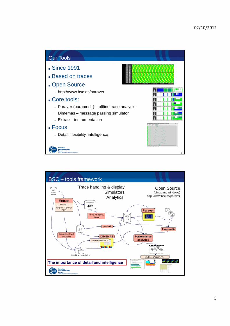
Our Tools

Since 1991

Based on traces

Open Source– http://www.bsc.es/paraver

Core tools:– Paraver (paramedir) – offline trace analysis

– Dimemas – message passing simulator

– Extrae – instrumentation

Focus– Detail, flexibility, intelligence

BSC – tools framework

CUBE, gnuplot, vi…

.prv+

.pcf

.trf

Time Analysis, filters

.cfg

Paramedir

.prv

Instruction level simulators

XMLcontrol

ParaverValgrind, Dyninst,

PAPI

MRNET

Extrae

DIMEMASVENUS (IBM-ZRL)

Machine description

Trace handling & displaySimulatorsAnalytics

Open Source (Linux and windows)

http://www.bsc.es/paraver

The importance of detail and intelligence

Performance analytics

prv2trf

.xls.txt

.cube

.plot

02/10/2012

6

Paraver

Multispectral imaging

Different looks at one reality– Different spectral bands (light sources and filters)

Highlight different aspects– Can combine into false colored but highly informative images

02/10/2012

7

13

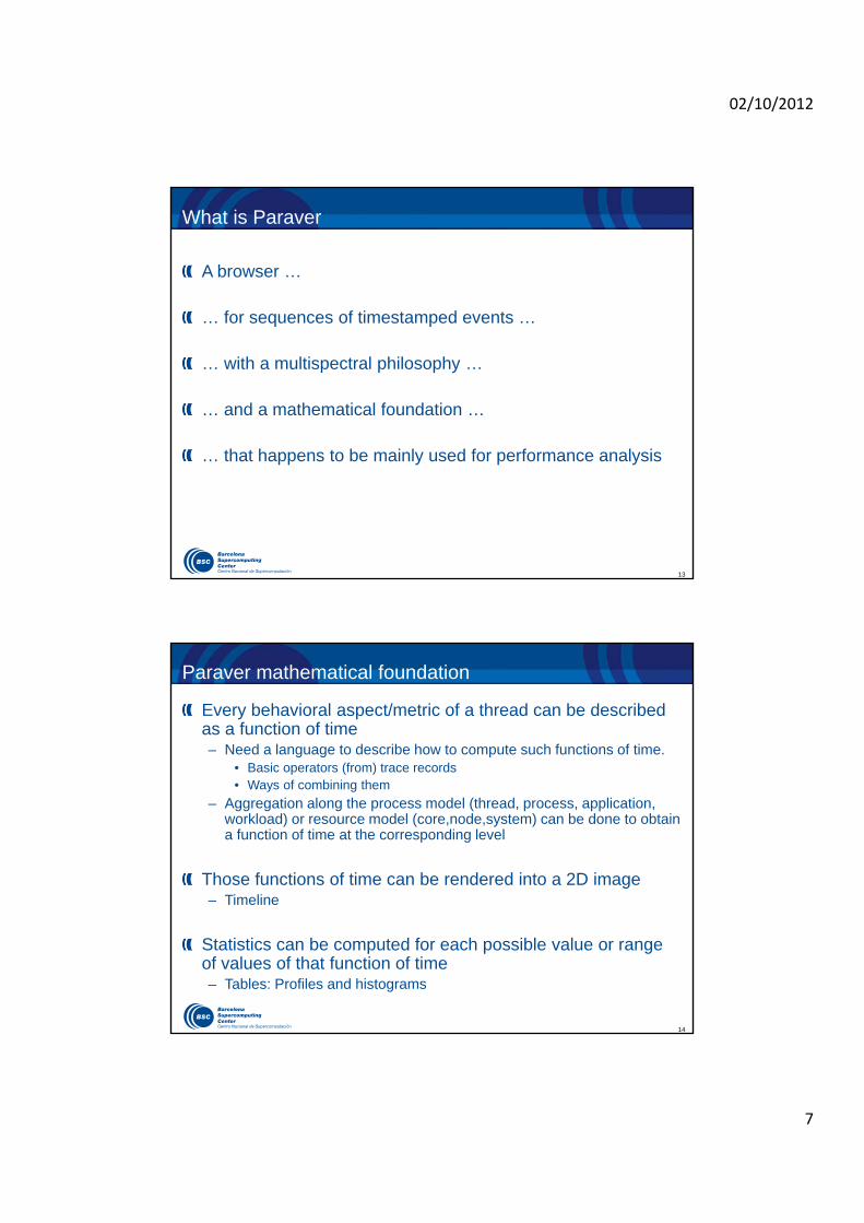
What is Paraver

A browser …

… for sequences of timestamped events …

… with a multispectral philosophy …

… and a mathematical foundation …

… that happens to be mainly used for performance analysis

14

Paraver mathematical foundation

Every behavioral aspect/metric of a thread can be described as a function of time– Need a language to describe how to compute such functions of time.

• Basic operators (from) trace records• Ways of combining them

– Aggregation along the process model (thread, process, application, workload) or resource model (core,node,system) can be done to obtain a function of time at the corresponding level

Those functions of time can be rendered into a 2D image – Timeline

Statistics can be computed for each possible value or range of values of that function of time– Tables: Profiles and histograms

02/10/2012

8

15

TImelines

Each window displays one view– Piecewise constant function of time– One such function of time per object:

• Thread, process, application, workload, CPU, node

Types of functions– Categorical

• State, user function, outlined routine

– Logical• In specific user function, In MPI call, In long MPI call

– Numerical• IPC, L2 miss ratio, Duration of MPI call, duration of computation

burst

nNSi ,n0,

1,,)( iii ttiStS

RSi

1 ,0 iS

16

Timelines

Representation– Function of time

– Color encoding

– Gradient color• Light green Dark blue

– Not null gradient• Black for zero value

• Light green Dark blue

Non linear rendering to address scalability

02/10/2012

9

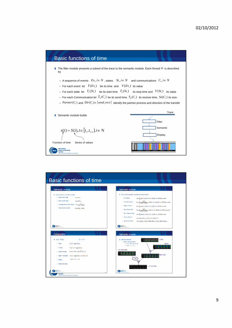
Basic functions of time

The filter module presents a subset of the trace to the semantic module. Each thread is described by

– A sequence of events , states and communications

– For each event let be its time and its value

– For each state let be its start time its stop time and its value

– For each Communication let be its send time, its receive time, its size.

– and identify the partner process and direction of the transfer

Semantic module builds

)( iR CT

itttiSts ii ,,),()( 1

NiEvi ,

)( iEvV)( iEvT

NiSti ,

)( is StT )( ie StT )( iStV

NiCi ,

)( iS CT )( iCSz

recvsendCDir i ,)(

Function of time Series of values

th

)( iCPartner

Filter

Semantic

Display

Trace

Basic functions of time

02/10/2012

10

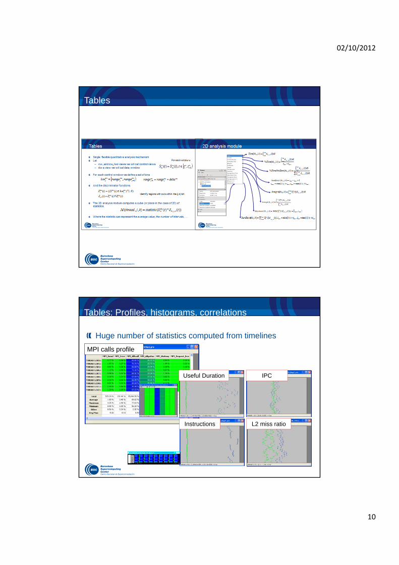
Tables

Tables: Profiles, histograms, correlations

Huge number of statistics computed from timelines

MPI calls profile

Useful Duration

Instructions

IPC

L2 miss ratio

02/10/2012

11

21

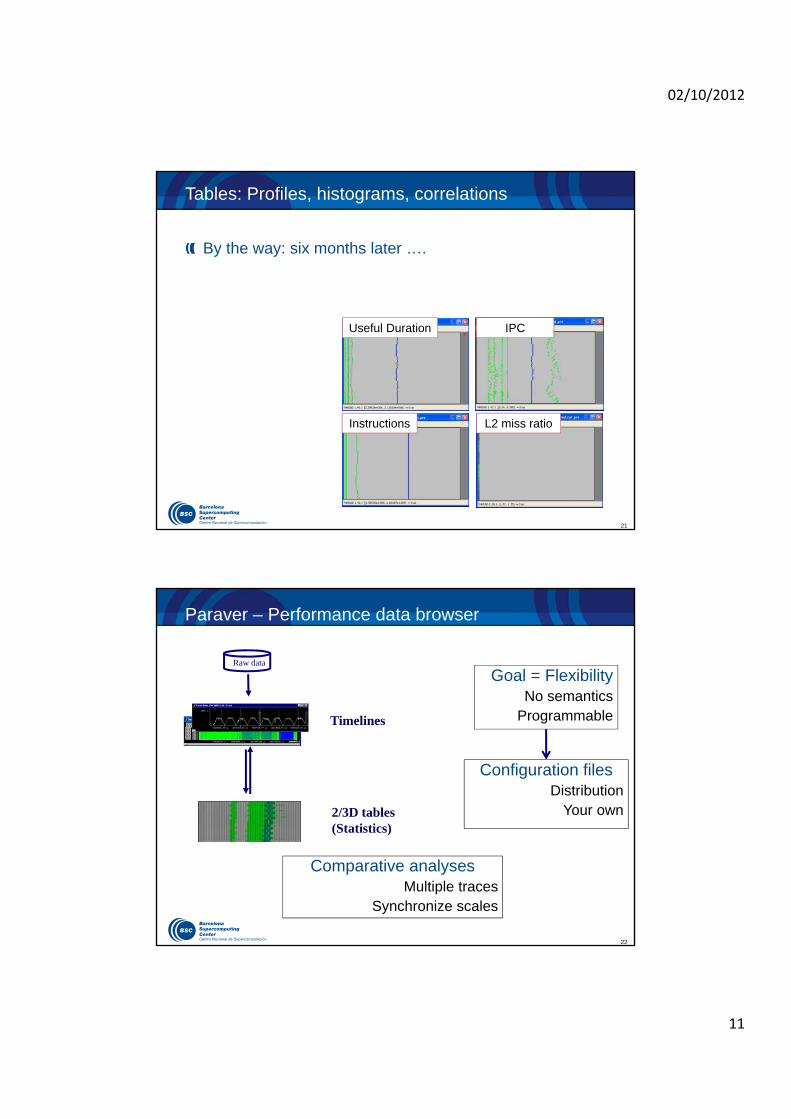
Tables: Profiles, histograms, correlations

By the way: six months later ….

Useful Duration

Instructions

IPC

L2 miss ratio

22

Paraver – Performance data browser

Timelines

Raw data

2/3D tables (Statistics)

Goal = FlexibilityNo semantics

Programmable

Configuration filesDistribution

Your own

Comparative analysesMultiple traces

Synchronize scales

02/10/2012

12

Paraver: finding needles in haystacks

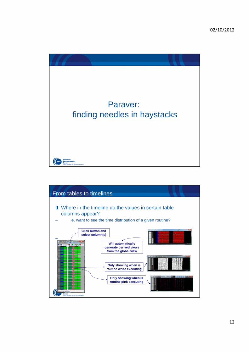
From tables to timelines

Where in the timeline do the values in certain table columns appear?

– ie. want to see the time distribution of a given routine?

–

Click button and select column(s)

Will automatically generate derived views

from the global view

Only showing when is routine pink executing

Only showing when is routine white executing

02/10/2012

13

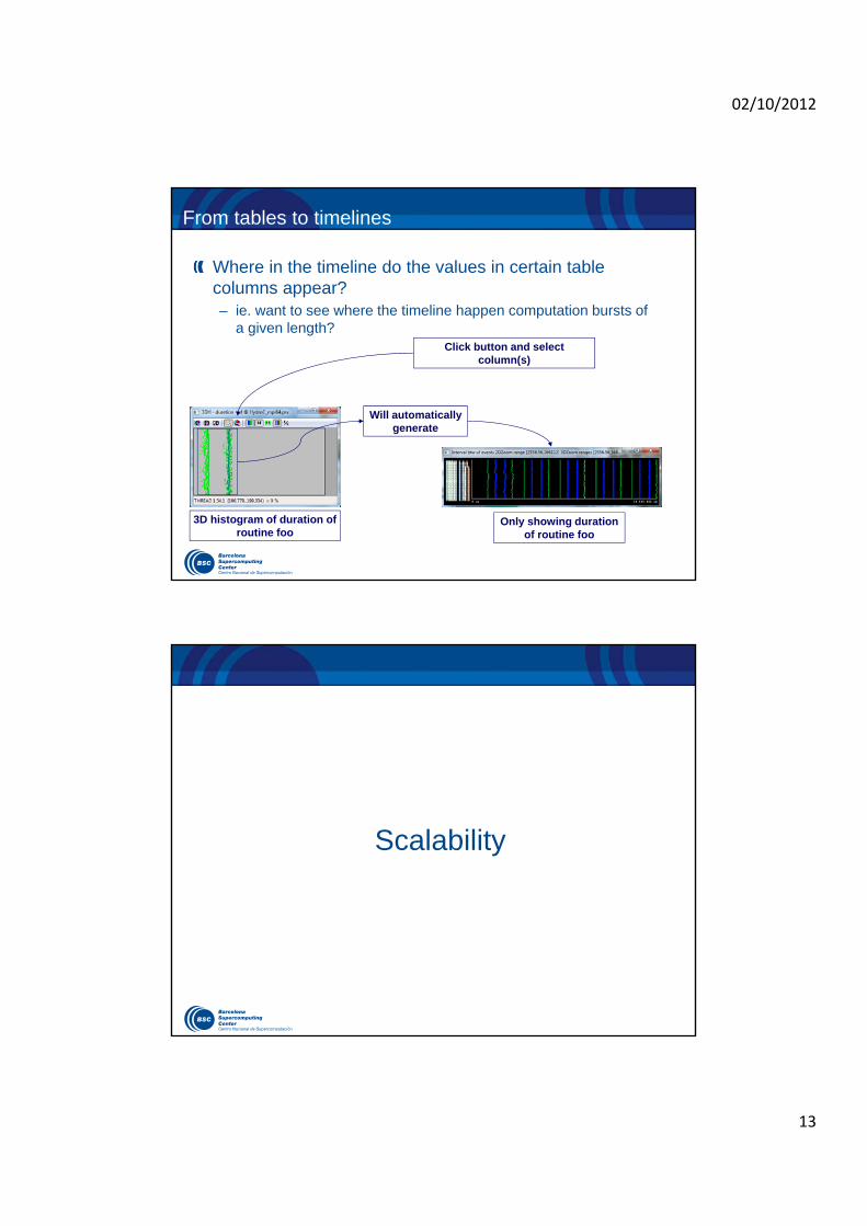
From tables to timelines

Where in the timeline do the values in certain table columns appear?– ie. want to see where the timeline happen computation bursts of

a given length?Click button and select

column(s)

Will automatically generate

3D histogram of duration of routine foo

Only showing duration of routine foo

Scalability

02/10/2012

14

27

Scalability of Presentation

Linpack @ Marenostrum: 10k cores x 1700 s

Dgemm IPC

2.95

2.85

Dgemm L1 miss ratio

0.8

0.7

Dgemm duration

11.8 s

10 s

Scalability of analysis

Jaguar

~ 47 seconds

Flow Tran

Jugene

~ 105 seconds

FlowTran

8K cores

12K cores

16K cores

PFLOTRAN

02/10/2012

15

29

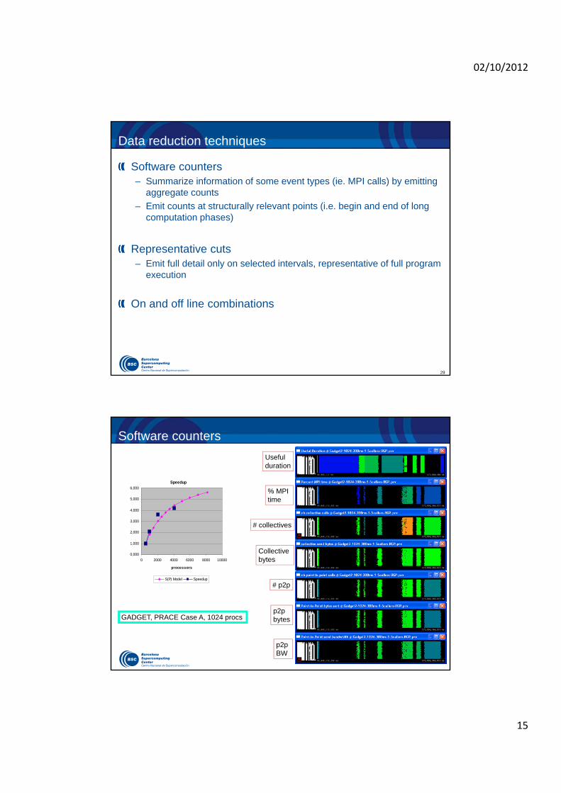
Data reduction techniques

Software counters– Summarize information of some event types (ie. MPI calls) by emitting

aggregate counts

– Emit counts at structurally relevant points (i.e. begin and end of long computation phases)

Representative cuts– Emit full detail only on selected intervals, representative of full program

execution

On and off line combinations

Software counters

Usefulduration

% MPI time

# collectives

Collective bytes

# p2p

p2p bytes

p2p BW

Speedup

0,000

1,000

2,000

3,000

4,000

5,000

6,000

0 2000 4000 6000 8000 10000

processors

S(P) Model Speedup

GADGET, PRACE Case A, 1024 procs

02/10/2012

16

Software countersUsefulduration

% MPI time

# collectives

Collective bytes

# p2p

p2p bytes

p2p BW

Speedup

0,000

1,000

2,000

3,000

4,000

5,000

6,000

0 2000 4000 6000 8000 10000

processors

S(P) Model Speedup

GADGET, PRACE Case A, 2048 procs

Software countersUsefulduration

% MPI time

# collectives

Collective bytes

# p2p

p2p bytes

p2p BW

Speedup

0,000

1,000

2,000

3,000

4,000

5,000

6,000

0 2000 4000 6000 8000 10000

processors

S(P) Model Speedup

GADGET, PRACE Case A, 4096 procs

02/10/2012

17

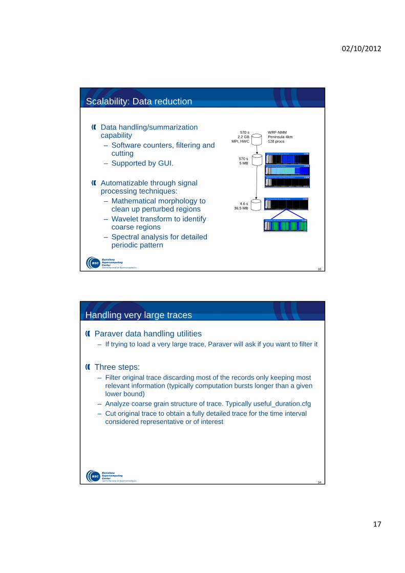
33

Data handling/summarization capability– Software counters, filtering and

cutting– Supported by GUI.

Automatizable through signal processing techniques:– Mathematical morphology to

clean up perturbed regions– Wavelet transform to identify

coarse regions– Spectral analysis for detailed

periodic pattern

570 s2.2 GB

MPI, HWC

WRF-NMMPeninsula 4km128 procs

570 s5 MB

4.6 s36.5 MB

Scalability: Data reduction

34

Handling very large traces

Paraver data handling utilities– If trying to load a very large trace, Paraver will ask if you want to filter it

Three steps:– Filter original trace discarding most of the records only keeping most

relevant information (typically computation bursts longer than a given lower bound)

– Analyze coarse grain structure of trace. Typically useful_duration.cfg

– Cut original trace to obtain a fully detailed trace for the time interval considered representative or of interest

02/10/2012

18

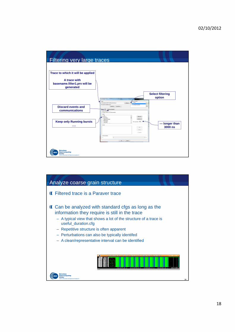
Filtering very large traces

Select filtering option

Discard events and communications

Trace to which it will be applied

A trace with basename.filter1.prv will be

generated

Keep only Running bursts ….

--- longer than 3000 ns

36

Analyze coarse grain structure

Filtered trace is a Paraver trace

Can be analyzed with standard cfgs as long as the information they require is still in the trace– A typical view that shows a lot of the structure of a trace is

useful_duration.cfg

– Repetitive structure is often apparent

– Perturbations can also be typically identifed

– A clean/representative interval can be identified

02/10/2012

19

37

Cutting very large traces

Load a filtered trace and use the scissors tool

Browse to select file from which the cut will

be obtained

Scissors tool

Click to select region

Select time interval by clicking left and right limits in a window of the

filtered trace previously loaded

Recommended cuts within long computation bursts

Select cutter

Default setups

38

Heterogeneous systems

GPUs

KNC: – OmpSs @ KNC ok.

– Still to be ported to intel accelerator model

OmpSsCholesky n = 8192; bs =1024

HMPP

MPI+CUDAHidro

02/10/2012

20

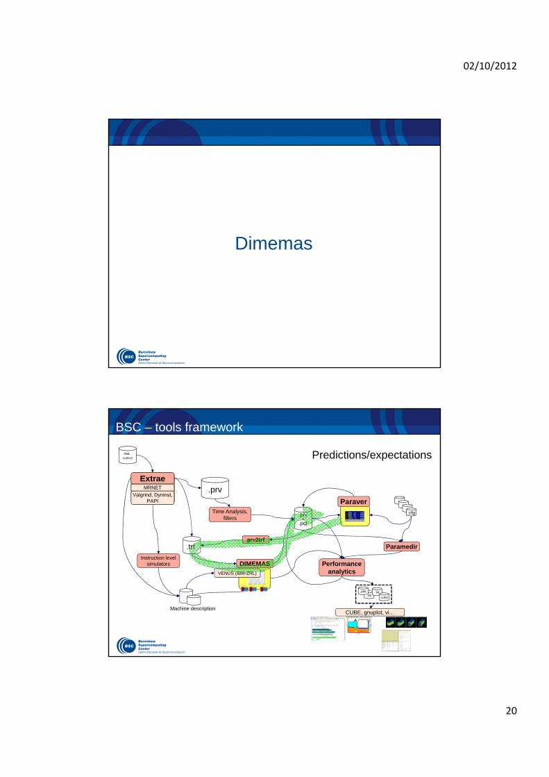
Dimemas

BSC – tools framework

CUBE, gnuplot, vi…

.prv+

.pcf

.trf

Time Analysis, filters

.cfg

Paramedir

.prv

Instruction level simulators

XMLcontrol

ParaverValgrind, Dyninst,

PAPI

MRNET

Extrae

DIMEMASVENUS (IBM-ZRL)

Machine description

Performance analytics

prv2trf

.xls.txt

.cube

.plot

Predictions/expectations

02/10/2012

21

41

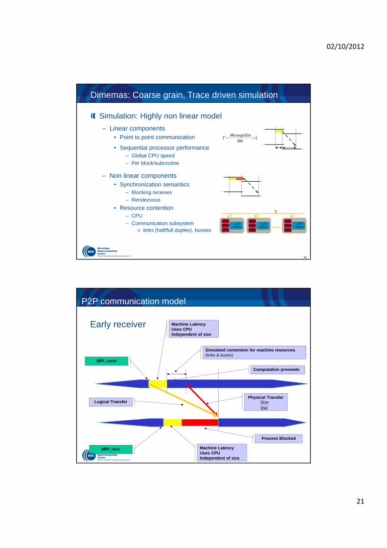
Dimemas: Coarse grain, Trace driven simulation

Simulation: Highly non linear model

– Linear components• Point to point communication

• Sequential processor performance– Global CPU speed

– Per block/subroutine

– Non linear components• Synchronization semantics

– Blocking receives

– Rendezvous

• Resource contention– CPU

– Communication subsystem » links (half/full duplex), busses

LBW

eMessageSizT

CPU

LocalMemory

B

CPU

CPU

L

CPU

CPU

CPULocal

Memory

L

CPU

CPU

CPULocal

Memory

L

P2P communication model

Early receiver

Simulated contention for machine resources (links & buses)

Physical Transfer

Process Blocked

BW

Size

Machine LatencyUses CPUIndependent of size

Computation proceeds

Machine LatencyUses CPUIndependent of size

Logical Transfer

MPI_send

MPI_recv

02/10/2012

22

43

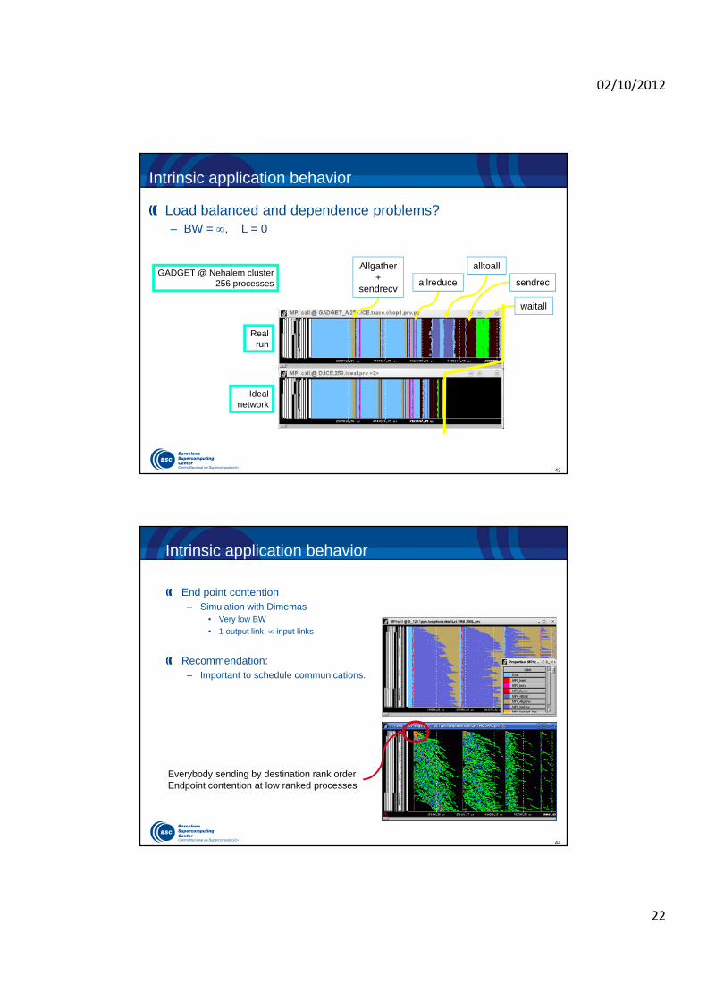
Intrinsic application behavior

Load balanced and dependence problems?– BW = , L = 0

waitall

sendrec

alltoall

Real run

Ideal network

Allgather+

sendrecvallreduce

GADGET @ Nehalem cluster256 processes

44

Intrinsic application behavior

End point contention– Simulation with Dimemas

• Very low BW

• 1 output link, input links

Recommendation:– Important to schedule communications.

Everybody sending by destination rank orderEndpoint contention at low ranked processes

02/10/2012

23

45

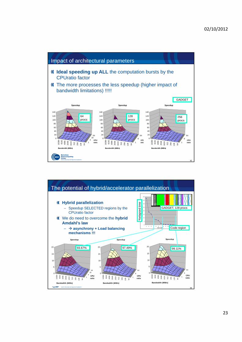
Impact of architectural parameters

Ideal speeding up ALL the computation bursts by the CPUratio factor

The more processes the less speedup (higher impact of bandwidth limitations) !!!!!

64

12

8

25

6

51

2

10

24

20

48

40

96

81

92

16

38

4

14

1664

0

20

40

60

80

100

120

140

Bandwidth (MB/s)

CPUratio

Speedup

64

12

8

25

6

51

2

10

24

20

48

40

96

81

92

16

38

4

1

8

64

0

20

40

60

80

100

120

140

Bandwidth (MB/s)

CPUratio

Speedup

64

12

8

25

6

51

2

10

24

20

48

40

96

81

92

16

38

4

1

8

64

0

20

40

60

80

100

120

140

Bandwidth (MB/s)

CPUratio

Speedup

64 procs

128 procs

256 procs

GADGET

46

The potential of hybrid/accelerator parallelization

Hybrid parallelization– Speedup SELECTED regions by the

CPUratio factor

We do need to overcome the hybrid Amdahl’s law – asynchrony + Load balancing

mechanisms !!!

Profile

0

5

10

15

20

25

30

35

40

1 2 3 4 5 6 7 8 9 10 11 12 13code region

% o

f co

mp

uta

tio

n t

ime

64

12

8

25

6

51

2

10

24

20

48

40

96

81

92

16

38

4

1

4

1664

0

5

10

15

20

Bandwdith (MB/s)

CPUratio

Speedup

64

12

8

25

6

51

2

10

24

20

48

40

96

81

92

16

38

4

1

8

64

0

5

10

15

20

Bandwdith (MB/s)

CPUratio

Speedup

64

12

8

25

6

51

2

10

24

20

48

40

96

81

92

16

38

4

1

8

64

0

5

10

15

20

Bandwdith (MB/s)

CPUratio

Speedup

93.67% 97.49% 99.11%

Code region

%el

apse

d tim

e

GADGET, 128 procs

02/10/2012

24

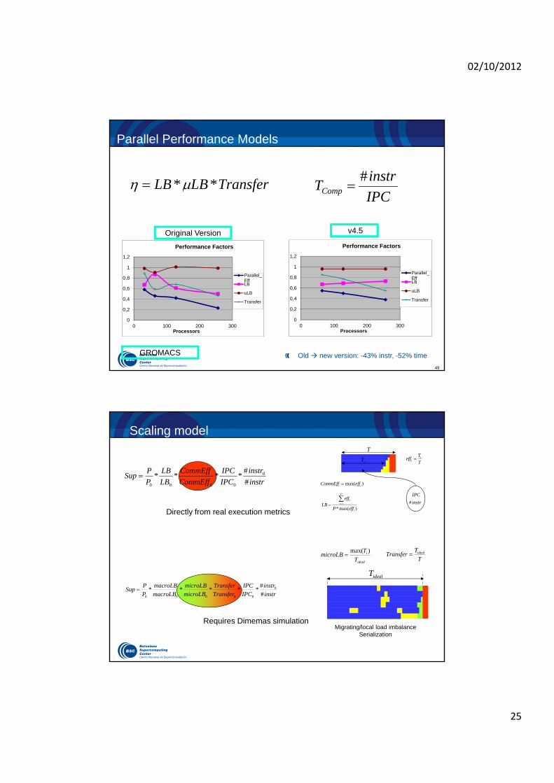
Scaling model

48

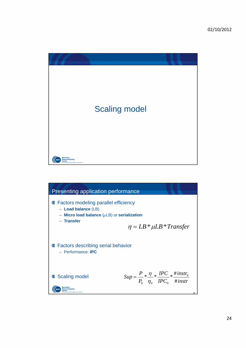
Presenting application performance

Factors modeling parallel efficiency– Load balance (LB)

– Micro load balance (LB) or serialization

– Transfer

Factors describing serial behavior– Performance: IPC

Scaling model

TransferLBLB **

instr

instr

IPC

IPC

P

PSup

#

#*** 0

000

02/10/2012

25

49

Parallel Performance Models

Old new version: -43% instr, -52% time

0

0,2

0,4

0,6

0,8

1

1,2

0 100 200 300Processors

Performance Factors

Parallel_EffLB

uLB

Transfer

0

0,2

0,4

0,6

0,8

1

1,2

0 100 200 300Processors

Performance Factors

Parallel_EffLB

uLB

Transfer

Original Version v4.5

GROMACS

TransferLBLB ** IPC

instrTComp

#

Scaling model

)max(*1

i

P

ii

effP

effLB

)max( ieffCommEff

T

Teff i

i iT

T

IPC

instr#

Directly from real execution metrics

instrinstr

IPCIPC

TransferTransfer

microLBmicroLB

macroLBmacroLB

PP

Sup##

***** 0

00000

Requires Dimemas simulationMigrating/local load imbalance

Serialization

idealT

T

TTransfer ideal

ideal

i

T

TmicroLB

)max(

instr

instr

IPC

IPC

CommEff

CommEff

LB

LB

P

PSup

#

#**** 0

0000

02/10/2012

26

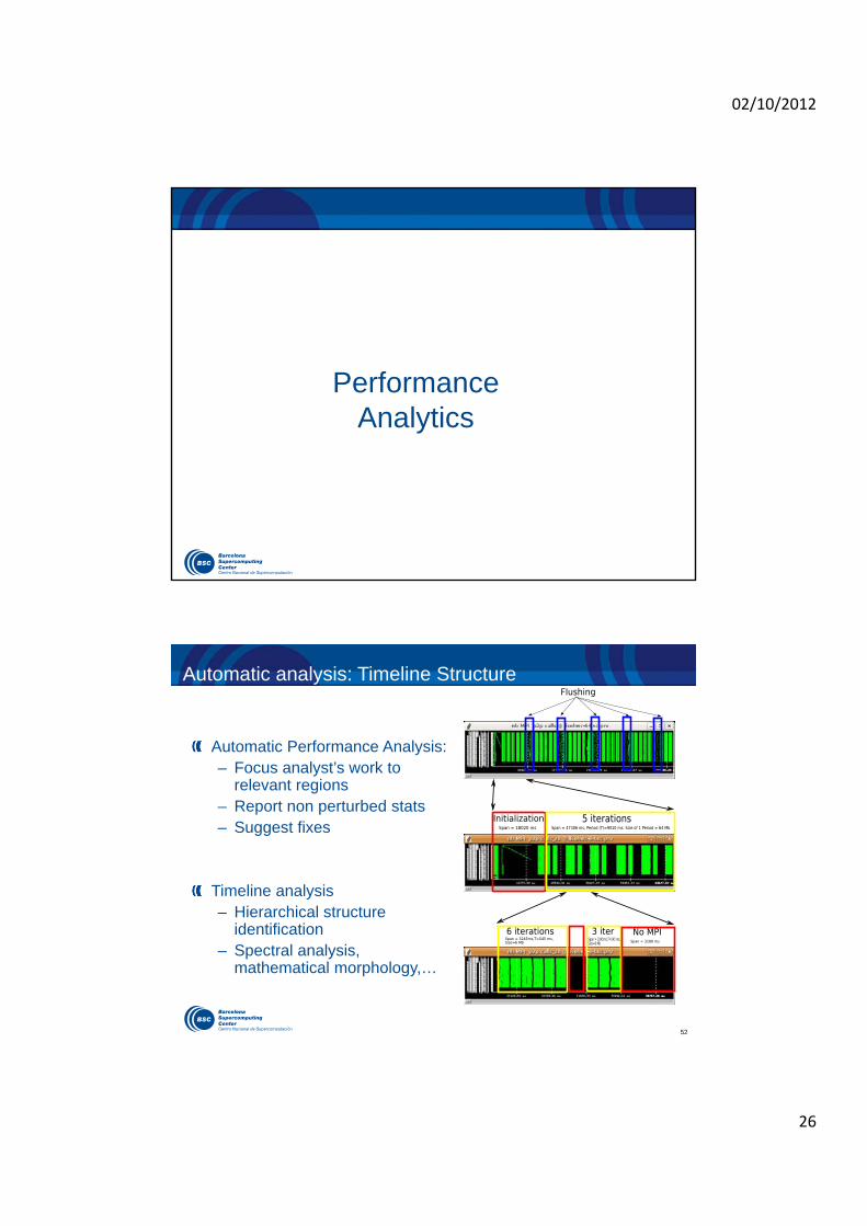
Performance Analytics

52

Automatic analysis: Timeline Structure

Automatic Performance Analysis:– Focus analyst’s work to

relevant regions– Report non perturbed stats– Suggest fixes

Timeline analysis– Hierarchical structure

identification – Spectral analysis,

mathematical morphology,…

02/10/2012

27

53

Signal processing applied to performance analysis

Identify structure

Reduce trace sizes

Increase precision of profiles

Flushing

Flushingfiltered

WaveletHigh

frequency

Useful Duration

Autocorrelation

Spectral density

T

Scalability: online automatic interval selection

“ G. Llort et all, “Scalable tracing with dynamic levels of detail”ICPADS 2011

T0

ClusteringAnalysis

MRNetFront-end

T1 Tn

…

Back-end threads

Aggregatedata

Broadcastresults

Structure detection

Detait trace only for smallinterval

02/10/2012

28

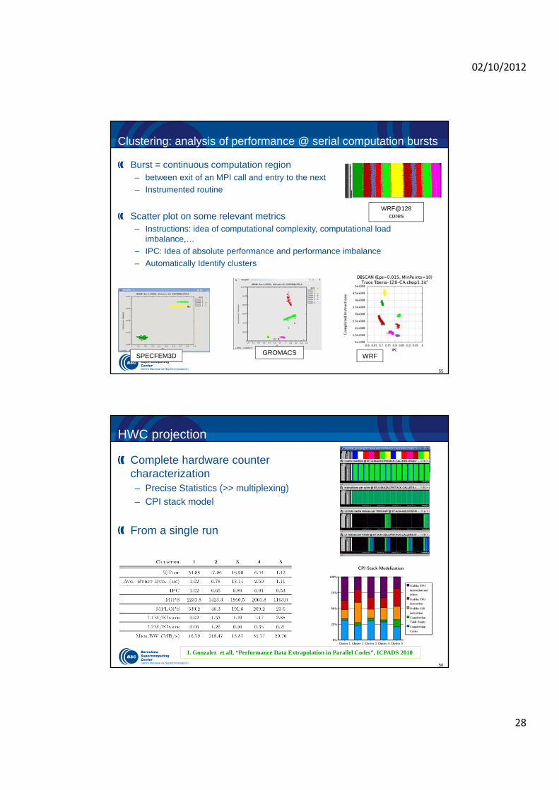
55

Clustering: analysis of performance @ serial computation bursts

Burst = continuous computation region – between exit of an MPI call and entry to the next

– Instrumented routine

Scatter plot on some relevant metrics– Instructions: idea of computational complexity, computational load

imbalance,…

– IPC: Idea of absolute performance and performance imbalance

– Automatically Identify clusters

WRFGROMACSSPECFEM3D

WRF@128 cores

56

Complete hardware counter characterization– Precise Statistics (>> multiplexing)

– CPI stack model

From a single run

HWC projection

J. Gonzalez et all, “Performance Data Extrapolation in Parallel Codes”, ICPADS 2010

02/10/2012

29

57

Automatic clustering quality assessment

Leverage Multiple Sequence alignment tools from Life Sciences

Process == Sequence of clusters sequence of amino acids == DNA

CLUSTAL W, T-Coffee, Kalign2

Cluster Sequence Score (0..1)

Per cluster / Global– Weighted average

BT.A0043

BT.A0022

58

Folding: Instrumentation + sampling

Extremely detailed time evolution of hardware counts, rates and callstack

Minimal overhead

Based on – Instrumentation events (iteration, MPI, …) and periodic samples.

– Application structure: manual iteration instrumentation, routines, clusters

Folding– Post processing to project all samples into one instance

0

0.2

0.4

0.6

0.8

1

0 0.2 0.4 0.6 0.8 1 0

100

200

300

400

500

600

700 0 0.2 0.4 0.6 0.8 1

Nor

mal

ized

com

mitt

ed in

stru

ctio

ns

MIP

S

Normalized time

Task 0 Thread 0 - tree_build.0Duration = 1233.49 ms Counter = 138486.13 Kinstructions

SamplesCurve fitting

Curve fitting slope

Detailed fine grain instructions within one

iteration

Original sampled instructions

Harald Servat et al. “Detailed performance analysis using coarse grain sampling” PROPER@EUROPAR, 2009

02/10/2012

30

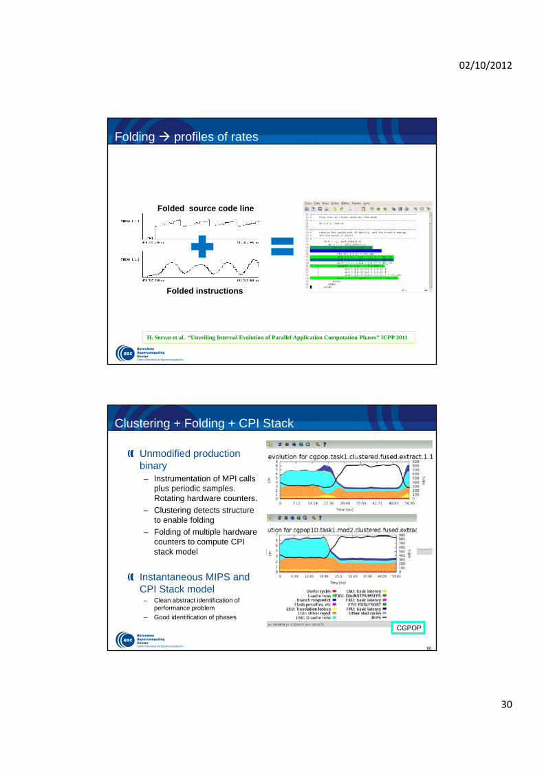
Folding profiles of rates

Folded source code line

Folded instructions

H. Servat et al. “Unveiling Internal Evolution of Parallel Application Computation Phases” ICPP 2011

60

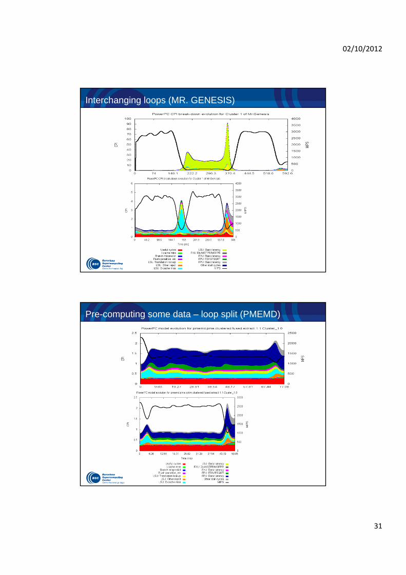
Clustering + Folding + CPI Stack

Unmodified production binary– Instrumentation of MPI calls

plus periodic samples. Rotating hardware counters.

– Clustering detects structure to enable folding

– Folding of multiple hardware counters to compute CPI stack model

Instantaneous MIPS and CPI Stack model

– Clean abstract identification of performance problem

– Good identification of phases

CGPOP

02/10/2012

31

Interchanging loops (MR. GENESIS)

Pre-computing some data – loop split (PMEMD)

02/10/2012

32

Tareador

64

Predicting performance

Performance prediction– Predict MPI/StarSs multithreaded from pure MPI

– Leveraging other tools in environment

Dimemas:Distributedmachine simulator

trace of MPI run

trace of MPI/SMPSs run

Original(MPI)execution

Potential(MPI+SMPSs)execution

MPI execution

Inputcode

codetranslation

mpicc

MPIprocess

MPIprocess

MPIprocess

Valgrindtracer

Valgrindtracer

Valgrindtracer

Incomplete/suggested taskification• pragmas • runtime calls (even on not well structured code)

02/10/2012

33

65

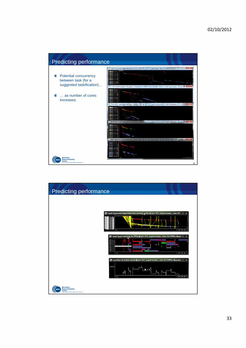
Predicting performance

Potential concurrency between task (for a suggested taskification)…

… as number of cores increases.

Predicting performance

02/10/2012

34

Conclusion

68

Conclusion

• Extreme flexibility:

• Maximize iterations of the hypothesis – validation loop

• Learning curve• “Don’t ask whether something can be done, ask how can it be done”

• Detailed and precise analysis

• Squeeze the information obtainable form a single run

• Insight and correct advise with estimates of potential gain

• Data analysis techniques applied to performance data

02/10/2012

35

69

Tools web site

www.bsc.es/paraver

• downloads– Sources

– Binaries

• documentation– Training guides (Documentation Paraver Introduction (MPI)

– Tutorial slides

70

An analogy

Use of traces

Huge probe effect

Multidisciplinary

Correlate different sources

Speculate till arriving to consistent theory

Team work