BROOKINGS DISCUSSION PAPERS IN INTERNATIONAL ECONOMICS

No. 124

ALTERNATIVE SPECIFICATIONS OF INTER- TEMPORAL FISCAL POLICY IN A SMALL THEORETICAL MODEL

Ralph C. Bryant and Long Zhang

June 1996

Ralph C. Bryant is a senior fellow in the Economic Studies Program of theBrookings Institution. Long Zhang is an economist in the Central Asia,Middle East and North Africa Department of the International FinanceCorporation. This paper is the second in a series of three working papers bythe same authors. The others are Bryant and Zhang (1996a, 1996c). Theoriginal research was conducted in 1993-94 and circulated in preliminaryform as a June 1994 draft entitled “Alternative Specifications ofIntertemporal Fiscal Policy in Macroeconomic Models: An Initial WorkingPaper.” Funding for the research came in part from the MacArthurFoundation. The views expressed are those of the authors and should not beinterpreted as reflecting the views of the trustees, officers or other staff of theBrookings Institution or the International Finance Corporation.

Brookings Discussion Papers in International Economics are circulated tostimulate discussion and critical comment. They have not been exposed tothe regular Brookings prepublication review and editorial process.References in publications to this material, other than acknowledgement bya writer who has had access to it, should be cleared with the author orauthors.

ABSTRACT

ALTERNATIVE SPECIFICATIONS OF INTERTEMPORAL FISCAL POLICY IN A SMALL THEORETICAL MODEL

Ralph C. Bryant and Long Zhang

In this second of a series of three working papers, we use a simple neoclassical growthmodel to illustrate how consumption, investment, and output -- more broadly, the entire dynamicequation system of a model -- can be strongly influenced by alternative specifications of areaction function describing the intertemporal behavior of a government’s fiscal authority. Theclasses of fiscal rule studied -- debt-stock targeting, incremental interest payments (IIP), and theanalytical benchmark of a balanced budget -- are described and discussed in the first paper in theseries. The analysis demonstrates that the consequences of shocks or policy actions can bestrongly conditioned by the intertemporal fiscal reaction function imposed on a macroeconomicmodel. Significant variation can occur for different types of rule, for alternative assumptionsabout the timing of the rule’s activation, and for alternative values of the rule’s feedbackcoefficients.

Ralph C. Bryant Long ZhangEconomic Studies Program Central Asia, Middle East & NorthBrookings Institution Africa Department1775 Mass. Ave., NW International Finance CorporationWashington, DC 20036 USA 1818 H Street, NWEmail: RBRYANT@BROOK.EDU Washington, DC 20433 USA

Email: LZHANG1@WORLDBANK.ORG

In both this and the first working paper, we treat as synonyms the expressions "fiscal1

reaction function" and "intertemporal fiscal closure rule" and sometimes for brevity speak simplyof a "fiscal rule." See the first paper for discussion.

Some friendly critics of our research have suggested that a somewhat different2

theoretical model -- for example, a two-period overlapping generations model that permitsintergenerational heterogeneity -- might have highlighted some of our points even more clearly.They may be right; we are agnostic on that point. The motive of our analysis is to stress pointsthat would emerge from a variety of expository models.

Productivity growth is assumed to be caused by labor-augmenting, Harrod-neutral3

technical progress. In growth models with exogenous productivity growth (technical progress),the productivity growth must be labor-augmenting for the model to have a steady state withconstant growth rates for the model’s variables; for discussion, see Barro and Sala-I-Martin(1995, pp. 54-55).

In this second working paper, we use a simple continuous-time neoclassical

growth model to illustrate how consumption, investment and output -- more broadly, the

entire dynamic equation system of a model -- can be strongly influenced by alternative

specifications of an intertemporal fiscal closure rule. The classes of fiscal rule studied --

debt-stock targeting, incremental interest payments (IIP), and the analytical benchmark of

a balanced budget -- are described and discussed in Bryant and Zhang (1996a).1

I. An Illustrative Simple Growth Model

Our simplified model is in the tradition of Yaari (1965), Blanchard (1985), Buiter

(1988), and Weil (1989). It is useful in qualitatively illustrating many of the conclusions

that deserve emphasis. We would not go so far as to assert that the model is the preferred

one for every aspect of the exposition. 2

The labor force in the model grows at a constant annual rate, n. For theoretical

simplicity, the labor force is treated as coterminous with the total population; in effect, all

individuals when born are of working age and immediately join the labor force.

Productivity grows at a constant rate B. Each agent, regardless of age, faces a constant3

Maxc(s,t)

U(s,t) / Etm4

te&2(i&t) u [c(s,i)] di

s. t. da(s,t)dt

' [r(t)%8] a(s,t)% w(s,t)& J(s,t)& c(s,t)

U (s,t)

k(s,t) b(s,t)

w(s,t) J(s,t)

2

(B1)

(B2)

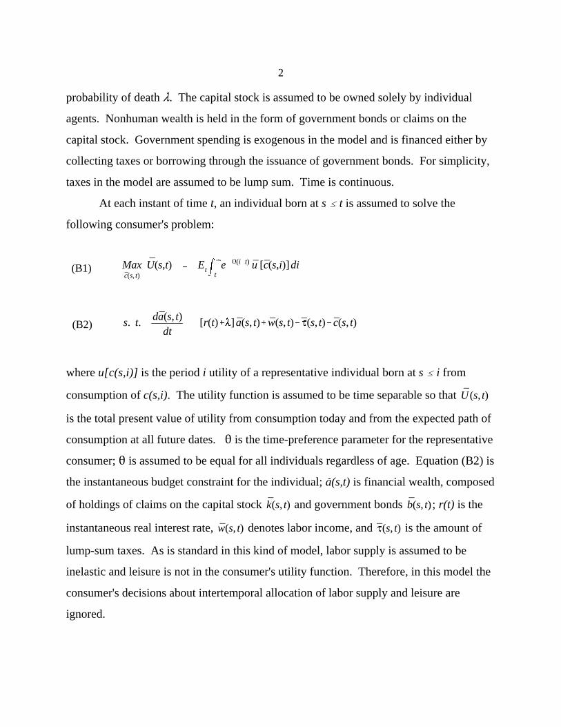
probability of death 8. The capital stock is assumed to be owned solely by individual

agents. Nonhuman wealth is held in the form of government bonds or claims on the

capital stock. Government spending is exogenous in the model and is financed either by

collecting taxes or borrowing through the issuance of government bonds. For simplicity,

taxes in the model are assumed to be lump sum. Time is continuous.

At each instant of time t, an individual born at s # t is assumed to solve the

following consumer's problem:

where u[c(s,i)] is the period i utility of a representative individual born at s # i from! !

consumption of c(s,i). The utility function is assumed to be time separable so that !

is the total present value of utility from consumption today and from the expected path of

consumption at all future dates. 2 is the time-preference parameter for the representative

consumer; 2 is assumed to be equal for all individuals regardless of age. Equation (B2) is

the instantaneous budget constraint for the individual; a(s,t) is financial wealth, composed!

of holdings of claims on the capital stock and government bonds ; r(t) is the

instantaneous real interest rate, denotes labor income, and is the amount of

lump-sum taxes. As is standard in this kind of model, labor supply is assumed to be

inelastic and leisure is not in the consumer's utility function. Therefore, in this model the

consumer's decisions about intertemporal allocation of labor supply and leisure are

ignored.

dhdt

' [r(t)%8] h(s,t)& [w(s,t)&J(s,t)]

dcdt' [r(t)&2] c(s,t)

c(s,t)' (2%8) [a(s,t)% h(s,t)]

h(s,t)/ m4

t[w(s,t)& J(s,t)] e

&mj

t(r i%8)di

dj .

h(s,t)

3

Logarithmic utility assumes that the intertemporal elasticity of substitution between4

consumption at two different dates is unity. This assumption is not appealing in its own right buthas the advantage of making the analysis more tractable. We relax this assumption in subsequentwork with small illustrative models.

(B3)

(B4)

(B5)

(B6)

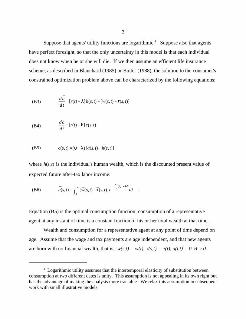
Suppose that agents' utility functions are logarithmic. Suppose also that agents4

have perfect foresight, so that the only uncertainty in this model is that each individual

does not know when he or she will die. If we then assume an efficient life insurance

scheme, as described in Blanchard (1985) or Buiter (1988), the solution to the consumer's

constrained optimization problem above can be characterized by the following equations:

where is the individual's human wealth, which is the discounted present value of

expected future after-tax labor income:

Equation (B5) is the optimal consumption function; consumption of a representative

agent at any instant of time is a constant fraction of his or her total wealth at that time.

Wealth and consumption for a representative agent at any point of time depend on

age. Assume that the wage and tax payments are age independent, and that new agents

are born with no financial wealth, that is, w(s,t) = w(t), J(s,t) = J(t), a(t,t) = 0 �t $ 0. ! ! ! ! !

c(t)' (2%8) [a(t)%h(t)]

0a(t)' [r& (n%B)] a(t)%w(t)&J(t)&c(t)

0h(t)' (r%8&B)h(t)%J(t)&w(t)

0c' [r& (2%B)] c(t)& (2%8)(n%8)a(t) .

f )(k(t))' r(t)

f (k(t))&k(t) r(t)'w(t)

4

For more explanation of the model's structure, see Zhang (1996).5

Perfect competition implies that all firms are price takers, both in the factor market and6

the goods market. Free entry and exit ensure that economic profits equal zero.

(B7)

(B8)

(B9)

(B10)

(B11)

(B12)

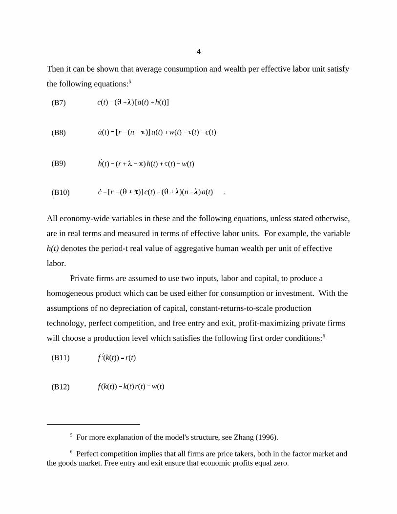
Then it can be shown that average consumption and wealth per effective labor unit satisfy

the following equations:5

All economy-wide variables in these and the following equations, unless stated otherwise,

are in real terms and measured in terms of effective labor units. For example, the variable

h(t) denotes the period-t real value of aggregative human wealth per unit of effective

labor.

Private firms are assumed to use two inputs, labor and capital, to produce a

homogeneous product which can be used either for consumption or investment. With the

assumptions of no depreciation of capital, constant-returns-to-scale production

technology, perfect competition, and free entry and exit, profit-maximizing private firms

will choose a production level which satisfies the following first order conditions:6

0b(t)% (n%B)b(t)'g(t)% r(t)b(t)&J(t) .

b(t)'m4

t[J(j)&g(j)] Rj dj .

c(t) ' (2%8) 6k(t)%m4

t[w(j)&g(j)] e

&mj

t[r(µ)%8&B] dµ

dj >

% (2%8)m4

t[J(j)&g(j)] Rj [1&e&(n%8)(j&t)] dj .

0k(t)' f(k(t))& (n%B)k(t)&g(t)&c(t) .

Rj'exp(&mj

t(rv& (n%B))dv)

limT64

b(T)Rj'0

5

(B13)

(B14)

(B15)

(B16)

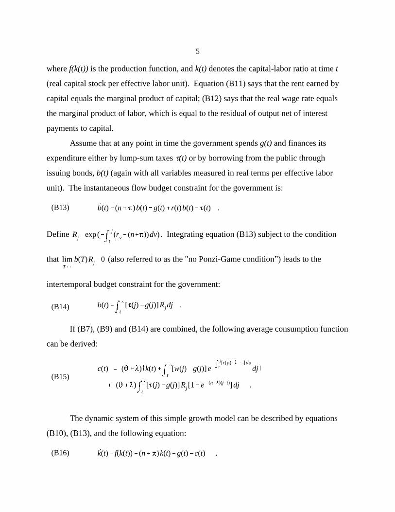
where f(k(t)) is the production function, and k(t) denotes the capital-labor ratio at time t

(real capital stock per effective labor unit). Equation (B11) says that the rent earned by

capital equals the marginal product of capital; (B12) says that the real wage rate equals

the marginal product of labor, which is equal to the residual of output net of interest

payments to capital.

Assume that at any point in time the government spends g(t) and finances its

expenditure either by lump-sum taxes J(t) or by borrowing from the public through

issuing bonds, b(t) (again with all variables measured in real terms per effective labor

unit). The instantaneous flow budget constraint for the government is:

Define . Integrating equation (B13) subject to the condition

that (also referred to as the "no Ponzi-Game condition”) leads to the

intertemporal budget constraint for the government:

If (B7), (B9) and (B14) are combined, the following average consumption function

can be derived:

The dynamic system of this simple growth model can be described by equations

(B10), (B13), and the following equation:

6g(j)>4t

m4

tJ(j)Rj dj

m4

t[w(j)&g(j)]e

&mj

t[r%8&B] dµ

dj

m4

t[J(j)&g(j)] Rj dj'0

6

When the special condition (n+8)=0 holds, the model exhibits full Ricardian7

equivalence. We exclude consideration of these special cases in this paper; for further discussionof this condition and the issues raised by Ricardian-equivalence propositions, see Zhang (1996).

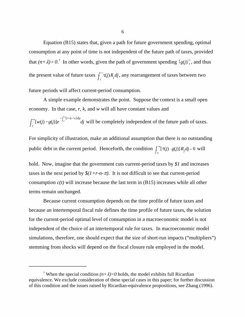
Equation (B15) states that, given a path for future government spending, optimal

consumption at any point of time is not independent of the future path of taxes, provided

that (n+8)� 0. In other words, given the path of government spending , and thus7

the present value of future taxes , any rearrangement of taxes between two

future periods will affect current-period consumption.

A simple example demonstrates the point. Suppose the context is a small open

economy. In that case, r, k, and w will all have constant values and

will be completely independent of the future path of taxes.

For simplicity of illustration, make an additional assumption that there is no outstanding

public debt in the current period. Henceforth, the condition will

hold. Now, imagine that the government cuts current-period taxes by $1 and increases

taxes in the next period by $(1+r-n-B). It is not difficult to see that current-period

consumption c(t) will increase because the last term in (B15) increases while all other

terms remain unchanged.

Because current consumption depends on the time profile of future taxes and

because an intertemporal fiscal rule defines the time profile of future taxes, the solution

for the current-period optimal level of consumption in a macroeconomic model is not

independent of the choice of an intertemporal rule for taxes. In macroeconomic model

simulations, therefore, one should expect that the size of short-run impacts (“multipliers”)

stemming from shocks will depend on the fiscal closure rule employed in the model.

[r (& (2%B)] c(

& (2%8)(n%8)a('0

f (k()& (n%B)k(&g(

&c('0

[r (& (n%B)] b(

%g(&J('0

7

Although average consumption (consumption per effective labor unit) is constant in the8

steady state, the consumption of each individual agent does change over his/her life cycle. Average consumption is always a constant share of total wealth (financial as well as humanwealth). But only in the steady state is average consumption a constant share of financial wealth.

(B17)

(B18)

(B19)

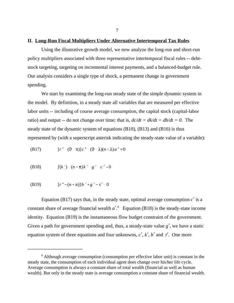
II. Long-Run Fiscal Multipliers Under Alternative Intertemporal Tax Rules

Using the illustrative growth model, we now analyze the long-run and short-run

policy multipliers associated with three representative intertemporal fiscal rules -- debt-

stock targeting, targeting on incremental interest payments, and a balanced-budget rule.

Our analysis considers a single type of shock, a permanent change in government

spending.

We start by examining the long-run steady state of the simple dynamic system in

the model. By definition, in a steady state all variables that are measured per effective

labor units -- including of course average consumption, the capital stock (capital-labor

ratio) and output -- do not change over time; that is, dc/dt = dk/dt = db/dt = 0. The

steady state of the dynamic system of equations (B10), (B13) and (B16) is thus

represented by (with a superscript asterisk indicating the steady-state value of a variable):

Equation (B17) says that, in the steady state, optimal average consumption c is a*

constant share of average financial wealth a . Equation (B18) is the steady-state income* 8

identity. Equation (B19) is the instantaneous flow budget constraint of the government.

Given a path for government spending and, thus, a steady-state value g , we have a static*

equation system of three equations and four unknowns, c , k , b and J . One more* * * *

dc(

dg(

'&

f ))(k()c(& (2%8) (n%8)A1

< 0

dJ(

dg(

'

A1% [r (& (2%B)] f ))(k()b(

A1

> 1

dk(

dg(

'

[r (& (2%B)] [ r (

& (n%B)]A1

< 0

A1' [r (& (2%B)] [ r (

& (n%B)]% f ))(k()c(&(2%8) (n%8)<0

8

The signs of the expressions are all determined as shown if one makes the reasonable9

assumption that r <n+ 2+8+B. This assumption is enforced for the numerical examples*

presented later. See Buiter (1988) or Zhang (1996) for a detailed discussion.

(B20)

(B22)

(B21)

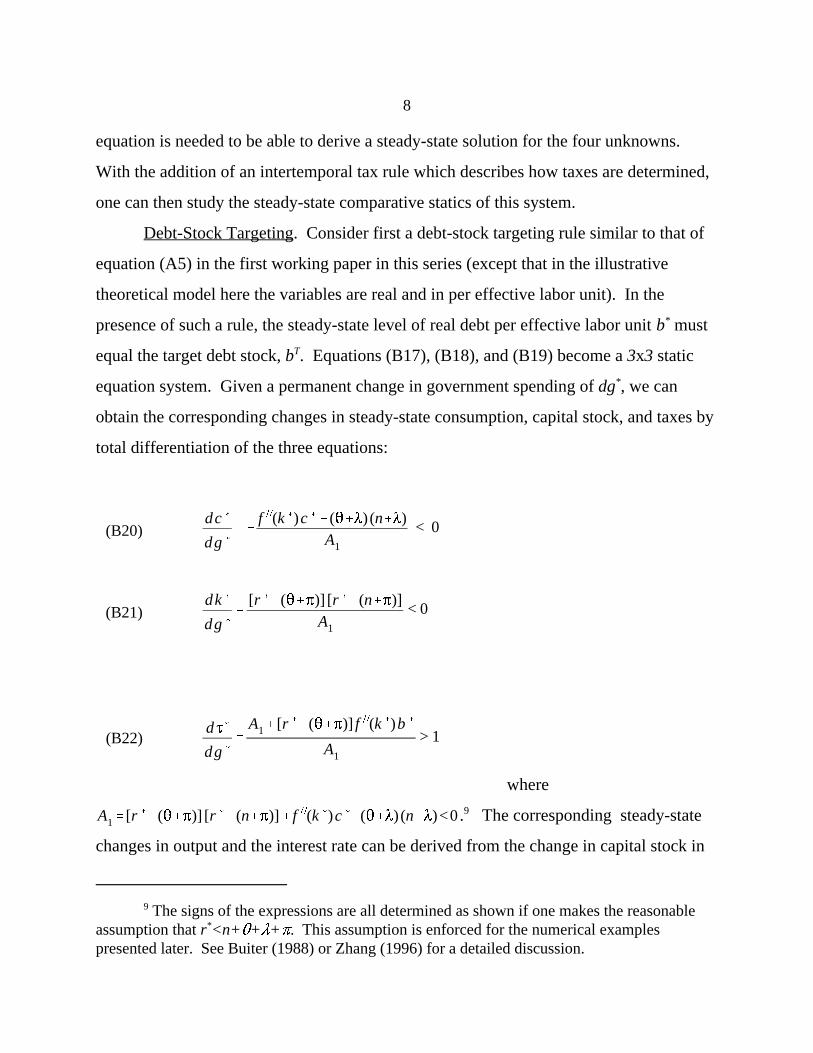
equation is needed to be able to derive a steady-state solution for the four unknowns.

With the addition of an intertemporal tax rule which describes how taxes are determined,

one can then study the steady-state comparative statics of this system.

Debt-Stock Targeting. Consider first a debt-stock targeting rule similar to that of

equation (A5) in the first working paper in this series (except that in the illustrative

theoretical model here the variables are real and in per effective labor unit). In the

presence of such a rule, the steady-state level of real debt per effective labor unit b must*

equal the target debt stock, b . Equations (B17), (B18), and (B19) become a 3x3 staticT

equation system. Given a permanent change in government spending of dg , we can*

obtain the corresponding changes in steady-state consumption, capital stock, and taxes by

total differentiation of the three equations:

where

. The corresponding steady-state9

changes in output and the interest rate can be derived from the change in capital stock in

dJ(

dg(

'

d(r (b()

dg(

9

In the Ricardian-equivalent case of (n+8)=0, dc /dg =-1 and dk /dg =0 and hence a10 * * * *

permanent change in government spending does not lead to any change in the steady-state capitalstock, investment, output and real interest rate. The increase in public consumption one-for-onedisplaces private consumption in the steady state. When (n+8) is substantially above zero, apermanent increase in government spending leads to substantial decreases in steady-state capitalstock, output and consumption.

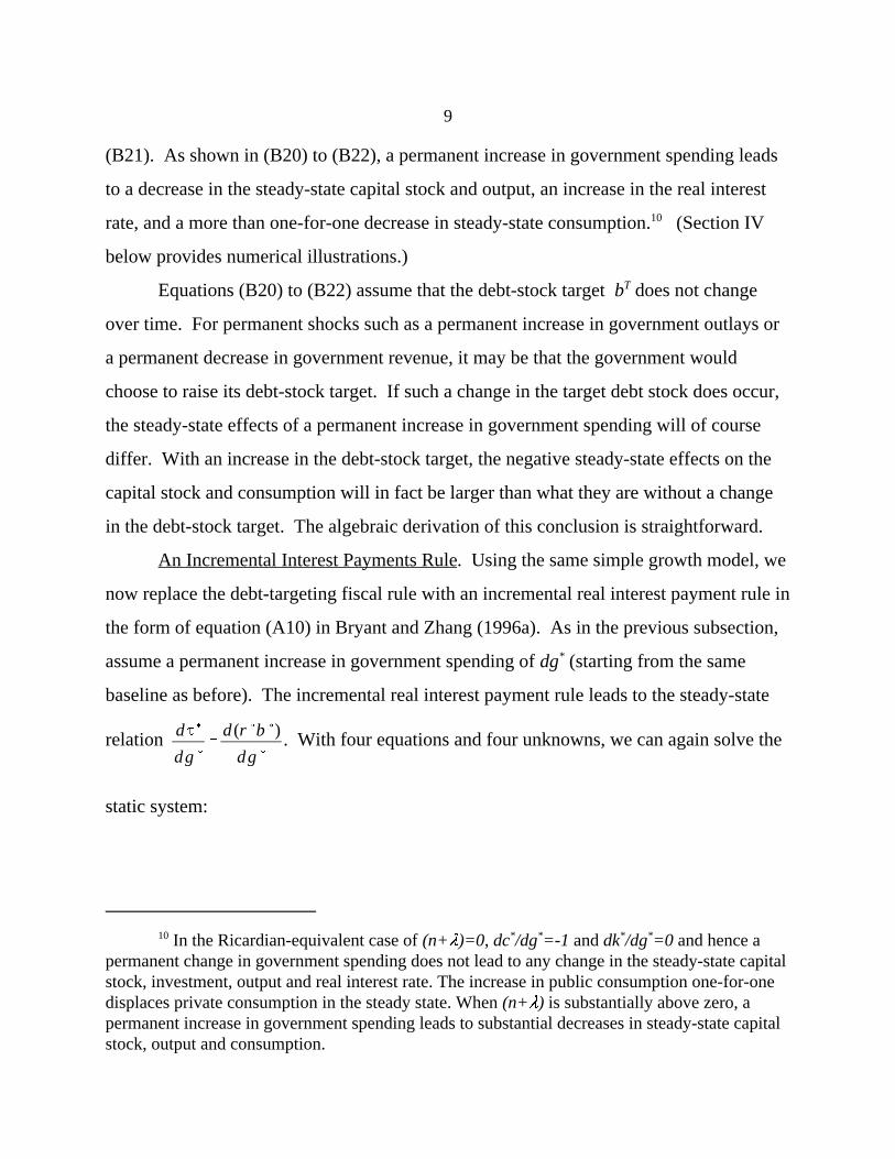
(B21). As shown in (B20) to (B22), a permanent increase in government spending leads

to a decrease in the steady-state capital stock and output, an increase in the real interest

rate, and a more than one-for-one decrease in steady-state consumption. (Section IV10

below provides numerical illustrations.)

Equations (B20) to (B22) assume that the debt-stock target b does not changeT

over time. For permanent shocks such as a permanent increase in government outlays or

a permanent decrease in government revenue, it may be that the government would

choose to raise its debt-stock target. If such a change in the target debt stock does occur,

the steady-state effects of a permanent increase in government spending will of course

differ. With an increase in the debt-stock target, the negative steady-state effects on the

capital stock and consumption will in fact be larger than what they are without a change

in the debt-stock target. The algebraic derivation of this conclusion is straightforward.

An Incremental Interest Payments Rule. Using the same simple growth model, we

now replace the debt-targeting fiscal rule with an incremental real interest payment rule in

the form of equation (A10) in Bryant and Zhang (1996a). As in the previous subsection,

assume a permanent increase in government spending of dg (starting from the same*

baseline as before). The incremental real interest payment rule leads to the steady-state

relation . With four equations and four unknowns, we can again solve the

static system:

dc(

dg(

'

[r (& (n%B)] (n%8) (2%8)

(n%B)A1

&

f ))(k()c(& (2%8) (n%8)A1

dk(

dg(

'

r (& (2%B)

A1

%

(2%8) (n%8)(n%B) A1

db(

dg(

'

1(n%B)

dJ(

dg(

'

[r (& (2%B)] f ))(k()b(

A1

%

r (A1% (2%8) (n%8) f ))(k()b(

(n%B) A1

.

10

(B23)(B24)(B25)(B26)

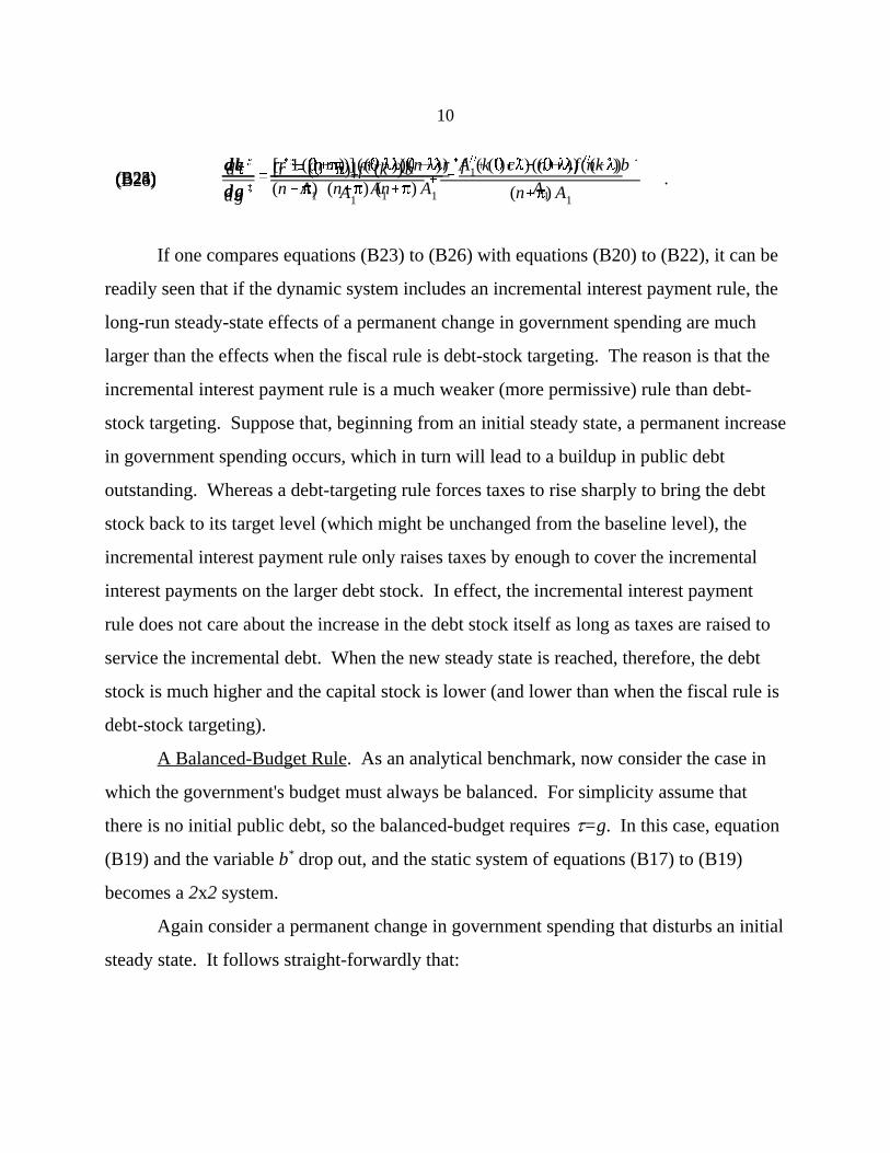
If one compares equations (B23) to (B26) with equations (B20) to (B22), it can be

readily seen that if the dynamic system includes an incremental interest payment rule, the

long-run steady-state effects of a permanent change in government spending are much

larger than the effects when the fiscal rule is debt-stock targeting. The reason is that the

incremental interest payment rule is a much weaker (more permissive) rule than debt-

stock targeting. Suppose that, beginning from an initial steady state, a permanent increase

in government spending occurs, which in turn will lead to a buildup in public debt

outstanding. Whereas a debt-targeting rule forces taxes to rise sharply to bring the debt

stock back to its target level (which might be unchanged from the baseline level), the

incremental interest payment rule only raises taxes by enough to cover the incremental

interest payments on the larger debt stock. In effect, the incremental interest payment

rule does not care about the increase in the debt stock itself as long as taxes are raised to

service the incremental debt. When the new steady state is reached, therefore, the debt

stock is much higher and the capital stock is lower (and lower than when the fiscal rule is

debt-stock targeting).

A Balanced-Budget Rule. As an analytical benchmark, now consider the case in

which the government's budget must always be balanced. For simplicity assume that

there is no initial public debt, so the balanced-budget requires J=g. In this case, equation

(B19) and the variable b drop out, and the static system of equations (B17) to (B19)*

becomes a 2x2 system.

Again consider a permanent change in government spending that disturbs an initial

steady state. It follows straight-forwardly that:

A1' [r (& (2%B)] [ r (

& (n%B)]% f ))(k()c(&(2%8) (n%8)<0

dc(

dg(

'

&[f ))(k()c(& (2%8) (n%8)]A1

dk(

dg(

'

r (& (2%B)

A1

11

A is still defined as . Since111

the steady-state values for r , c , and k are different, however, the value of A is different.* * *1

(B27)(B28)

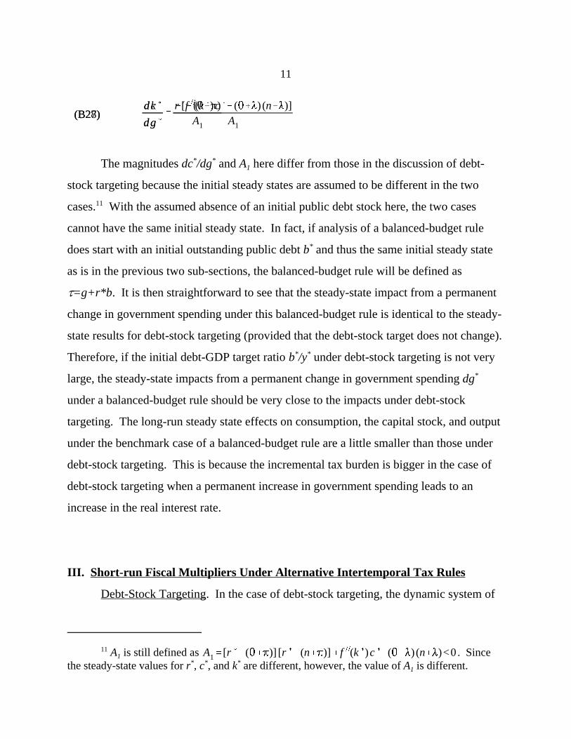
The magnitudes dc /dg and A here differ from those in the discussion of debt-* *1

stock targeting because the initial steady states are assumed to be different in the two

cases. With the assumed absence of an initial public debt stock here, the two cases11

cannot have the same initial steady state. In fact, if analysis of a balanced-budget rule

does start with an initial outstanding public debt b and thus the same initial steady state*

as is in the previous two sub-sections, the balanced-budget rule will be defined as

J=g+r*b . It is then straightforward to see that the steady-state impact from a permanent

change in government spending under this balanced-budget rule is identical to the steady-

state results for debt-stock targeting (provided that the debt-stock target does not change).

Therefore, if the initial debt-GDP target ratio b /y under debt-stock targeting is not very* *

large, the steady-state impacts from a permanent change in government spending dg*

under a balanced-budget rule should be very close to the impacts under debt-stock

targeting. The long-run steady state effects on consumption, the capital stock, and output

under the benchmark case of a balanced-budget rule are a little smaller than those under

debt-stock targeting. This is because the incremental tax burden is bigger in the case of

debt-stock targeting when a permanent increase in government spending leads to an

increase in the real interest rate.

III. Short-run Fiscal Multipliers Under Alternative Intertemporal Tax Rules

Debt-Stock Targeting. In the case of debt-stock targeting, the dynamic system of

dcdt

dkdt

dbdt

dJdt

'

r (&2&B c(f ))&(n%8)(2%8) &(n%8)(2%8) 0

&1 r (&n&B 0 0

0 f ))b( r (&n&B &1

0 "2b( f )) "1%"2(r (&n&B) &"2

c&c(

k&k(

b&b(

J&J(

%

0

&)g(t)

)g(t)

"2)g(t)

) c(0)'&[D1& (r (&2&B)])G(D1)%

(n%8)(2%8) D1)G(D1)

D21%["2&(r&n&B)]D1%"1

12

The same methodology can be applied to study the short-run impacts of most fiscal12

shocks, both transitory and permanent. Zhang (1996) provides details.

In the case of two conjugate complex eigenvalues, the real parts of the two complex13

roots must be negative.

(B29)

(B30)

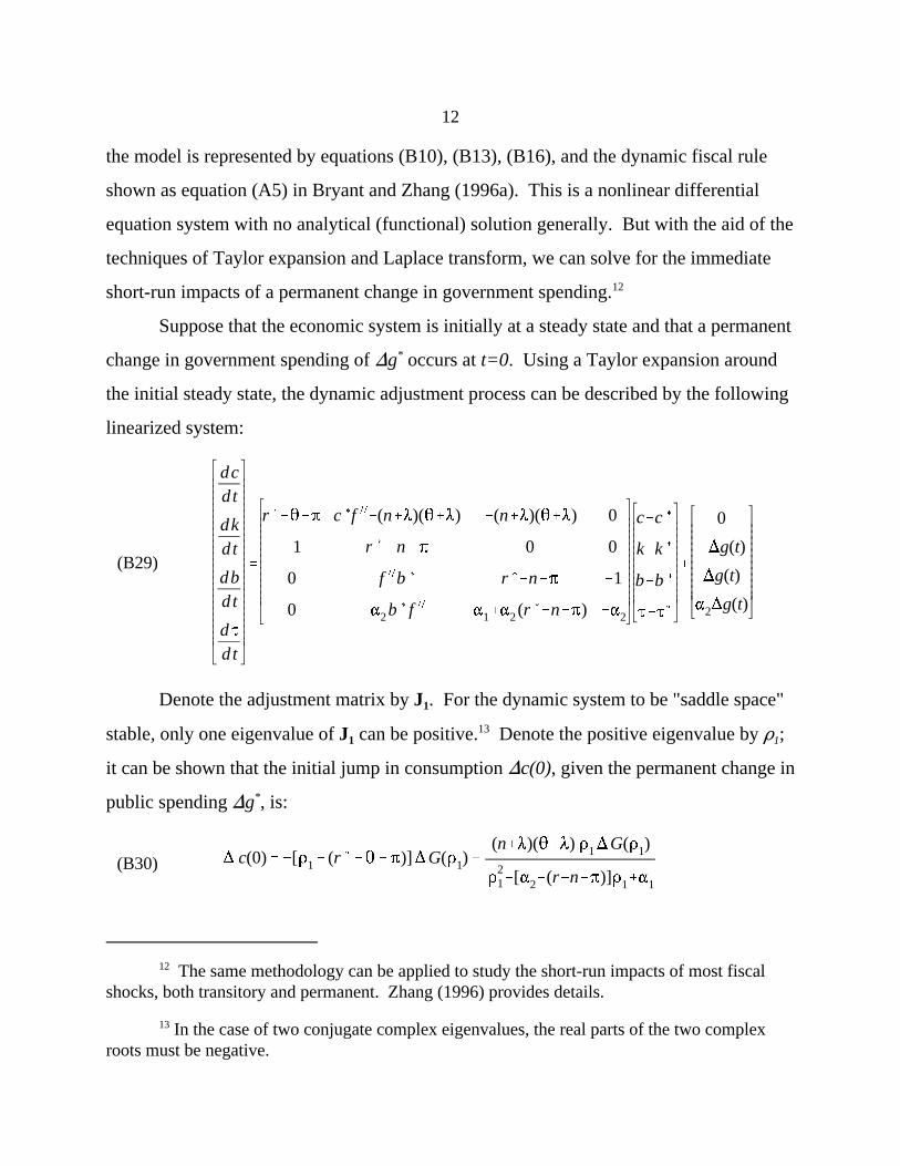
the model is represented by equations (B10), (B13), (B16), and the dynamic fiscal rule

shown as equation (A5) in Bryant and Zhang (1996a). This is a nonlinear differential

equation system with no analytical (functional) solution generally. But with the aid of the

techniques of Taylor expansion and Laplace transform, we can solve for the immediate

short-run impacts of a permanent change in government spending.12

Suppose that the economic system is initially at a steady state and that a permanent

change in government spending of )g occurs at t=0. Using a Taylor expansion around*

the initial steady state, the dynamic adjustment process can be described by the following

linearized system:

Denote the adjustment matrix by J . For the dynamic system to be "saddle space"1

stable, only one eigenvalue of J can be positive. Denote the positive eigenvalue by D ;113

1

it can be shown that the initial jump in consumption )c(0), given the permanent change in

public spending )g , is:*

0k(0)' &)c(0)& )g(0)

)G(x)'m4

0e&xt)g(t)dt

13

Note that )k(0)=0, )b(0)=0. State variables can not jump on impact when a fiscal14

policy change, )g(t), is announced. Therefore, )f(k), = 0 and )c(0)+k(0)+)g(0)=0. t=0"

In the Ricardian-equivalence cases in which (n+8)=0, r =2+B and (B30) collapses to15 *

)c(0)=-)g . A permanent increase in government spending leads to an immediate one-for-one*

drop in private consumption and leaves everything else unchanged.

(B31)

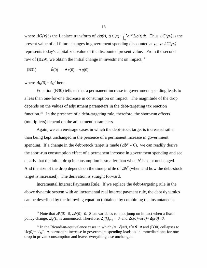
where )G(x) is the Laplace transform of )g(t), . Thus )G(D ) is the1

present value of all future changes in government spending discounted at D ; D )G(D )1 1 1

represents today's capitalized value of the discounted present value. From the second

row of (B29), we obtain the initial change in investment on impact,14

where )g(0)=)g here.*

Equation (B30) tells us that a permanent increase in government spending leads to

a less than one-for-one decrease in consumption on impact. The magnitude of the drop

depends on the values of adjustment parameters in the debt-targeting tax reaction

function. In the presence of a debt-targeting rule, therefore, the short-run effects15

(multipliers) depend on the adjustment parameters.

Again, we can envisage cases in which the debt-stock target is increased rather

than being kept unchanged in the presence of a permanent increase in government

spending. If a change in the debt-stock target is made ()b � 0), we can readily deriveT

the short-run consumption effect of a permanent increase in government spending and see

clearly that the initial drop in consumption is smaller than when b is kept unchanged. T

And the size of the drop depends on the time profile of )b (when and how the debt-stockT

target is increased). The derivation is straight forward.

Incremental Interest Payments Rule. If we replace the debt-targeting rule in the

above dynamic system with an incremental real interest payment rule, the debt dynamics

can be described by the following equation (obtained by combining the instantaneous

0b'& (n%B)b%g&J(% r (b( .

dcdt

dkdt

dbdt

'

r (&2&B c(f ))& (n%8)(2%8) &(n%8)(2%8)

&1 r (&n&B 0

0 0 &(n%B)

c&c(

k&k(

b&b(

%

0

&)g(t)

)g(t)

) c(0)'&[D2& (r (&2&B)])G(D2)%

(n%8) (2%8)D2%n%B

)G(D2) .

14

The steady-state baseline values in equations (A10) and (A11) are denoted with16

overbars rather than, as here, with asterisks. Recall that all variables in the illustrative model ofthis paper are expressed in per effective labor units.

(B32)

(B33)

(B34)

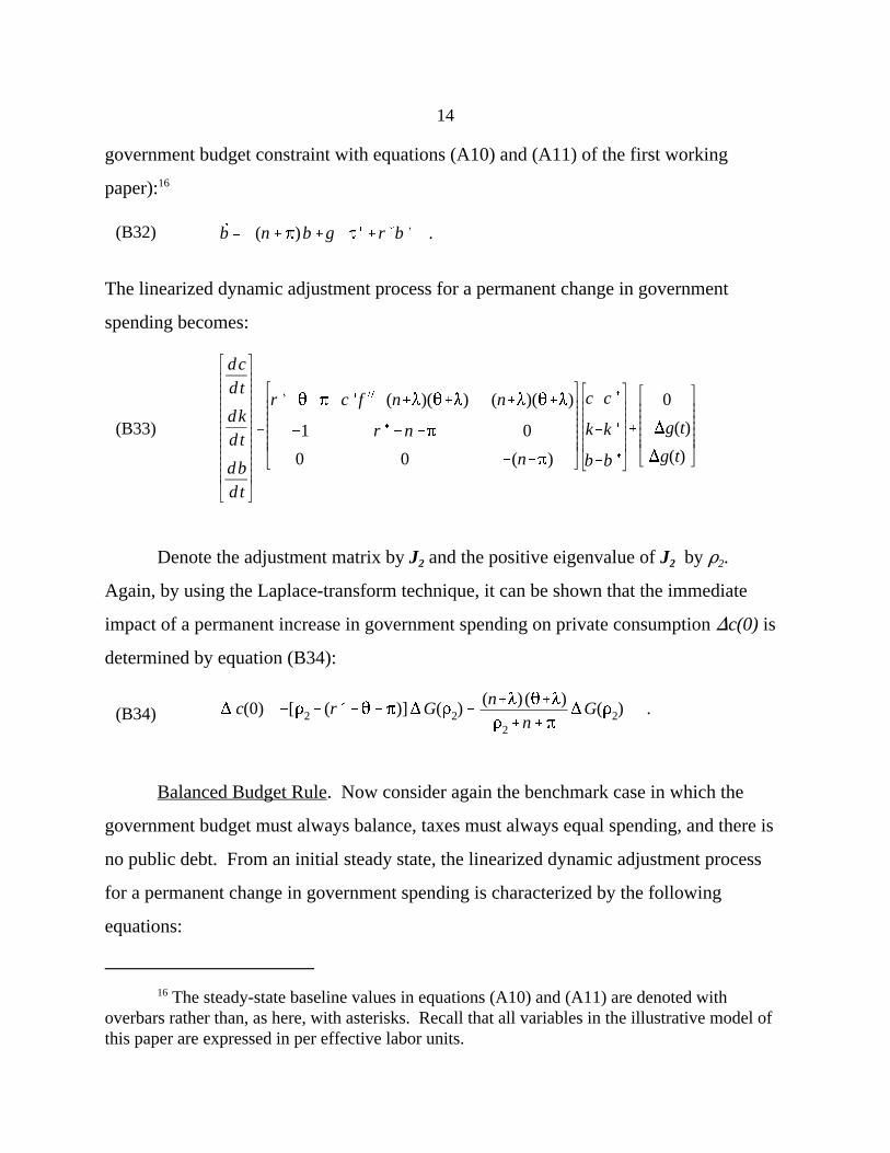
government budget constraint with equations (A10) and (A11) of the first working

paper):16

The linearized dynamic adjustment process for a permanent change in government

spending becomes:

Denote the adjustment matrix by J and the positive eigenvalue of J by D . 2 2 2

Again, by using the Laplace-transform technique, it can be shown that the immediate

impact of a permanent increase in government spending on private consumption )c(0) is

determined by equation (B34):

Balanced Budget Rule. Now consider again the benchmark case in which the

government budget must always balance, taxes must always equal spending, and there is

no public debt. From an initial steady state, the linearized dynamic adjustment process

for a permanent change in government spending is characterized by the following

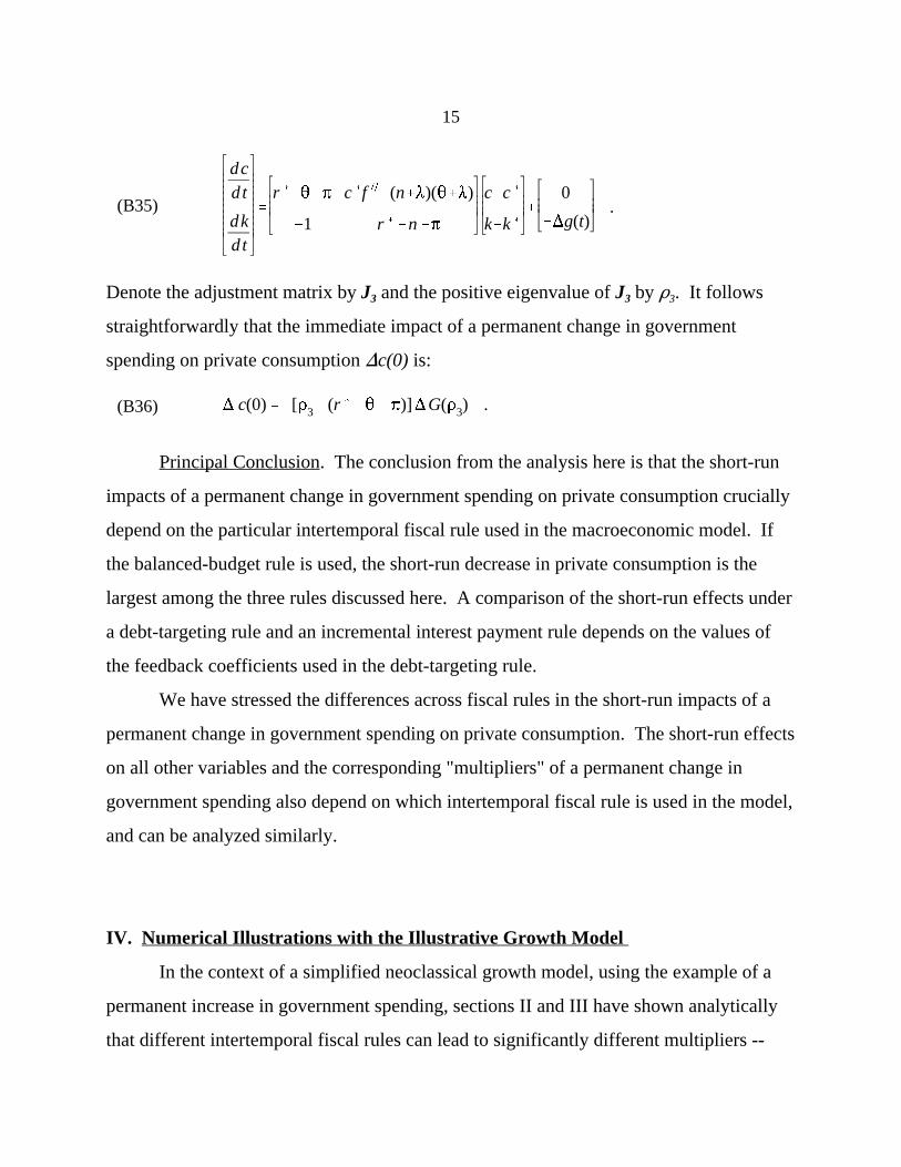
equations:

dcdt

dkdt

'

r (&2&B c(f ))& (n%8)(2%8)

&1 r (&n&B

c&c(

k&k(

%

0

&)g(t).

) c(0)'&[D3& (r (&2&B)])G(D3) .

15

(B35)

(B36)

Denote the adjustment matrix by J and the positive eigenvalue of J by D . It follows3 3 3

straightforwardly that the immediate impact of a permanent change in government

spending on private consumption )c(0) is:

Principal Conclusion. The conclusion from the analysis here is that the short-run

impacts of a permanent change in government spending on private consumption crucially

depend on the particular intertemporal fiscal rule used in the macroeconomic model. If

the balanced-budget rule is used, the short-run decrease in private consumption is the

largest among the three rules discussed here. A comparison of the short-run effects under

a debt-targeting rule and an incremental interest payment rule depends on the values of

the feedback coefficients used in the debt-targeting rule.

We have stressed the differences across fiscal rules in the short-run impacts of a

permanent change in government spending on private consumption. The short-run effects

on all other variables and the corresponding "multipliers" of a permanent change in

government spending also depend on which intertemporal fiscal rule is used in the model,

and can be analyzed similarly.

IV. Numerical Illustrations with the Illustrative Growth Model

In the context of a simplified neoclassical growth model, using the example of a

permanent increase in government spending, sections II and III have shown analytically

that different intertemporal fiscal rules can lead to significantly different multipliers --

16

both for the long-run steady state and for the short run. We now report numerical

illustrations obtained from several types of simulations with the simplified model. These

simulations highlight other aspects of the differences between the alternative

specifications of fiscal rules and provide a basis for preliminary judgment about the

quantitative importance of these differences.

Discrete-Time Version of the Model and its Calibration. To carry out the

numerical simulations, we first construct a discrete-time version of the continuous-time

model presented earlier. For easy reference, the discrete-time version incorporating debt-

stock targeting is summarized in Figure B-1. Eight variables -- consumption, the capital

stock, output, the interest rate, human wealth, the tax rate, tax revenues, and the stock of

government debt -- are determined endogenously, all measured in real terms per effective

labor unit. Government expenditures, G, and a target path for the debt stock, BT (each

also measured in real terms per effective labor unit) are exogenous variables. The key

parameters include the rate of growth of population (labor force), n; the rate of time

preference, 2; the rate of labor-augmenting technical progress, B; and the probability of

death, 8.

The left-hand panel in Figure B-1 shows the steady-state form of the model’s

equations. The right-hand panel gives the dynamic form used in the simulations. The

production function, the first equation, is implemented as Cobb-Douglas (with the share

of capital equal to 0.3). The second equation sets the real rate of interest equal to the

marginal product of capital. The fourth equation determines tax revenues as the product

of the tax rate and income. The fifth and sixth equations are the consumption and

forward-looking human-wealth functions, discussed in earlier sections. The final two

equations are the identities for national income and the government’s budget.

The third equation shown in Figure B-1 is the tax-rate reaction function, a variant

of debt-stock targeting discussed in the first working paper; " and " are the feedback1 2

coefficients on, respectively, the proportional and the derivative terms. The formulation

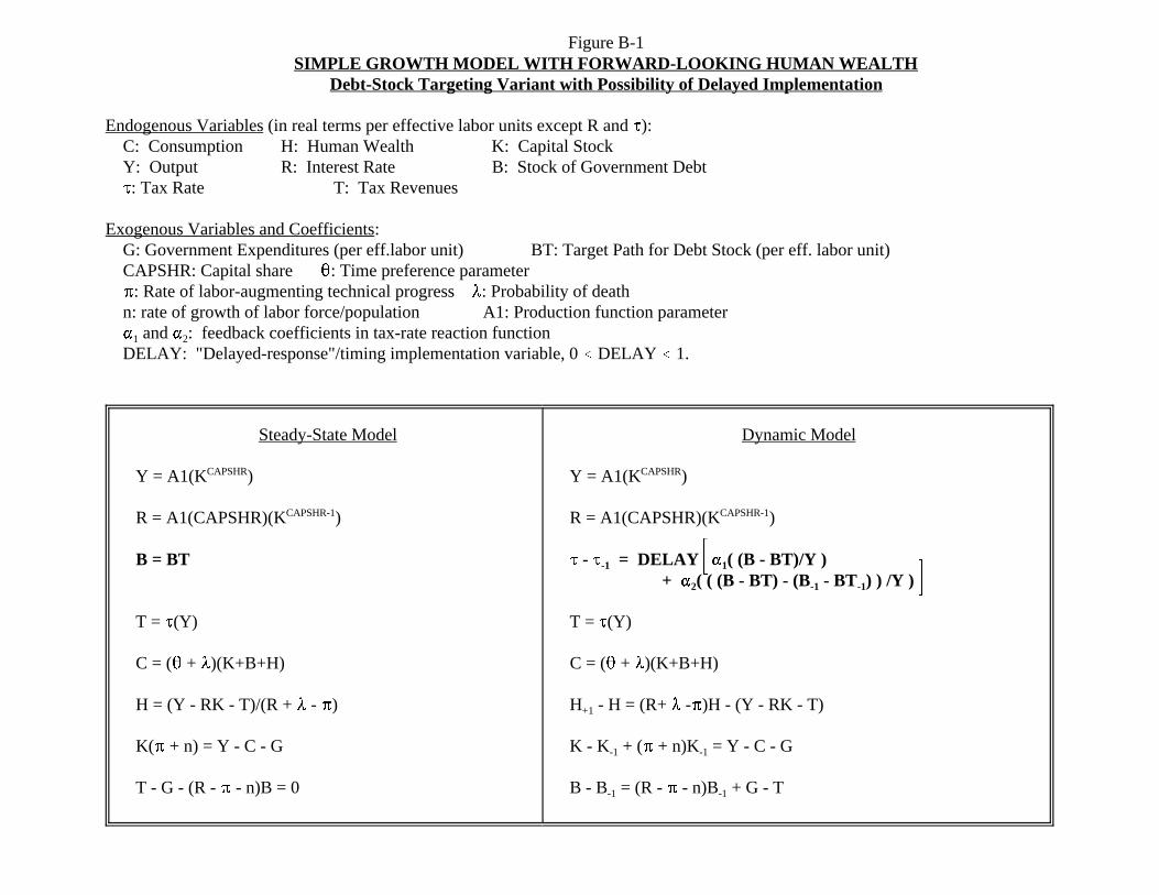
Figure B-1SIMPLE GROWTH MODEL WITH FORWARD-LOOKING HUMAN WEALTH

Debt-Stock Targeting Variant with Possibility of Delayed Implementation

Endogenous Variables (in real terms per effective labor units except R and J): C: Consumption H: Human Wealth K: Capital Stock Y: Output R: Interest Rate B: Stock of Government Debt J: Tax Rate T: Tax Revenues

Exogenous Variables and Coefficients: G: Government Expenditures (per eff.labor unit) BT: Target Path for Debt Stock (per eff. labor unit) CAPSHR: Capital share 2: Time preference parameter B: Rate of labor-augmenting technical progress 8: Probability of death n: rate of growth of labor force/population A1: Production function parameter " and " : feedback coefficients in tax-rate reaction function 1 2

DELAY: "Delayed-response"/timing implementation variable, 0 # DELAY # 1.

Steady-State Model Dynamic Model

Y = A1(K ) Y = A1(K )CAPSHR

R = A1(CAPSHR)(K ) R = A1(CAPSHR)(K )CAPSHR-1

B = BT JJ - JJ = DELAY "" ( (B - BT)/Y )

T = J(Y) T = J(Y)

C = (2 + 8)(K+B+H) C = (2 + 8)(K+B+H)

H = (Y - RK - T)/(R + 8 - B) H - H = (R+ 8 -B)H - (Y - RK - T)

K(B + n) = Y - C - G K - K + (B + n)K = Y - C - G

T - G - (R - B - n)B = 0 B - B = (R - B - n)B + G - T

CAPSHR

CAPSHR-1

-1 1�� + "" ( ( (B - BT) - (B - BT ) ) /Y ) 2 -1 -1 ��

+1

-1 -1

-1 -1

17

in Figure B-1 also provides for the possibility of non-unity values for the DELAY termt

(see section II of Bryant and Zhang (1996a) for general discussion). Simulations making

use of this DELAY term are reported below.t

For the model versions incorporating the alternative fiscal reaction functions, the

debt-stock-targeting equation shown in Figure B-1 is of course replaced by the

appropriate specification for the other rule (either incremental interest payments or the

balanced budget).

For the initial calibration of the simulation model, we select the following values

for the key parameters: n = 0.01, 8 = 0.04, 2 = 0.05, and B = 0.015. Values for G and BT,

respectively, are 100 and 175. In the initial steady state, government spending is

approximately 22 percent of income, tax revenues are approximately 25 percent of

income, the debt-income ratio is 39 percent, human wealth is about four times the size of

income, and private consumption is 69 percent of income.

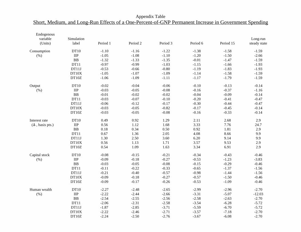
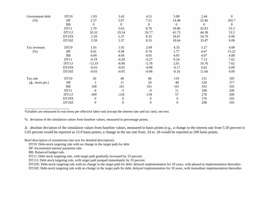
In what follows, we rely primarily on graphs to report the simulation results. In an

appendix table, however, we also provide numerical results for several of the main

simulations. The appendix table reports values for periods 1, 2, 3, 6, 15, and the eventual

long-run steady state. The graphs focusing on the short and medium run show results for

the first 20 periods; graphs reporting results for longer horizons show 40 or sometimes

100 periods. In both the graphs and the appendix table, results are shown as deviations

from a baseline simulation. For most of the variables, for example consumption and the

capital stock, the reported values are percentage deviations from baseline. For the interest

rate and the tax rate, the figures are absolute deviations from baseline. (The symbol %

indicates percent deviation from baseline and ) indicates absolute deviation from

baseline.)

The simulations are performed using the Portable TROLL software developed and

marketed by INTEX Solutions Incorporated. Our graphs are prepared with the cellVision

spreadsheet and database manager developed for use with GAUSS by Tom Bok and

18

Warwick McKibbin (McKibbin Software Group Inc.).

Comparison of Debt-Stock-Targeting, IIP, and Balanced-Budget Rules. We begin

by shocking the model with a standardized, one-percent-of-GDP, permanent increase in

government spending. Three variants of the model are used, one each for the debt-stock-

targeting, the IIP, and the balanced-budget fiscal rules. The simulation with the Debt-

stock Targeting rule is given the label DT10 (the “1" as the third character in the label

indicates that government expenditure is being changed from its baseline path, and "0" as

the fourth character indicates that the target path for the debt stock is not being changed).

The two feedback coefficients in the debt-targeting rule are given the values " = 0.041

and " = 0.30. The label IIP denotes the Incremental real Interest Payment rule and the2

BB label denotes the results for the analytical benchmark case in which the total budget is

always balanced.

Consider first the long-run steady-state effects for the DT10, IIP, and BB

simulations, reported in Table B-1. (For the time being, ignore the rows in Table B-1

labeled DT11 and DT11J; these will be discussed shortly.) Under debt-stock targeting,

steady-state private consumption decreases by 1.59%, output decreases by 0.14%, and the

real interest rate increases by 2.9 basis points. Alternatively, if the incremental real

interest payment rule is used in the same model, the increase in government spending

leads to a 2.66% decrease in steady-state consumption, a 1.16% fall in steady-state output,

and a 24.7 basis points increase in the real interest rate. The long-run steady-state

impacts of the increase in government spending differ substantially between these two

intertemporal fiscal rules.

The debt-targeting rule and the balanced-budget rule in this illustration have

exactly the same long-run effects. This is because we assume that the initial steady-state

debt stock in the BB scenario is exactly equal to the debt-stock target in the DT10 case;

thus the DT10 and BB scenarios always have the same steady-state solutions. Even if we

do not allow any government borrowing in the balanced-budget case (so that public debt

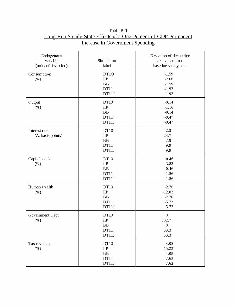
Table B-1Long-Run Steady-State Effects of a One-Percent-of-GDP Permanent

Increase in Government Spending

Endogenous Deviation of simulationvariable Simulation steady state from

(units of deviation) label baseline steady state

Consumption DT1O -1.59(%) IIP -2.66

BB -1.59DT11 -1.93DT11J -1.93

Output DT10 -0.14(%) IIP -1.16

BB -0.14DT11 -0.47DT11J -0.47

Interest rate DT10 2.9 (), basis points) IIP 24.7

BB 2.9 DT11 9.9DT11J 9.9

Capital stock DT10 -0.46(%) IIP -3.83

BB -0.46DT11 -1.56DT11J -1.56

Human wealth DT10 -2.70(%) IIP -12.03

BB -2.70DT11 -5.72DT11J -5.72

Government Debt DT10 0(%) IIP 202.7

BB 0DT11 33.3DT11J 33.3

Tax revenues DT10 4.08(%) IIP 15.22

BB 4.08DT11 7.62DT11J 7.62

19

is always zero), the steady-state impacts under the BB rule will still be similar to the

steady-state impacts under debt-stock targeting. This similarity is primarily due to the

fact that the target value for debt under the DT10 rule is assumed equal to the initial

baseline level of debt and that initial level itself is not large.

If the target path for the debt stock under debt targeting is raised rather than kept

unchanged when government spending permanently increases, the difference in outcomes

between the debt-stock targeting and BB rules then of course becomes significant. This

point can be seen clearly by contrasting the DT10 and BB simulations with two additional

simulations, labeled DT11 and DT11J. Government expenditures in all four simulations

are increased by 1 percent of baseline GDP. In the DT11 and DT11J simulations,

however, the target paths for the debt stock are also increased above baseline, by 33

percent. For the DT11J simulation (the "J" indicating a jump change), the debt-stock

target is immediately and permanently increased by the 33% starting from the first period

of the simulation. For the DT11 simulation, the target path for the debt stock is raised

gradually over the first 15 periods (eventually increasing by the 33% by the 15th period

and thereafter permanently maintained at that higher level).

The DT11J and DT11 simulations of course produce identical results for the long-

run steady state. But those two have noticeably different steady-state impacts from the

DT10 and BB simulations. When the long-run debt-stock target is increased by 33%, a

1%-of-GDP permanent increase in government spending leads to a reduction in steady-

state private consumption by 1.93%, a decrease in steady-state output by 0.47%, and an

increase in the steady-state real interest rate of about 10 basis points. Clearly, changes in

the debt target can have major consequences for long-run steady-state impacts.

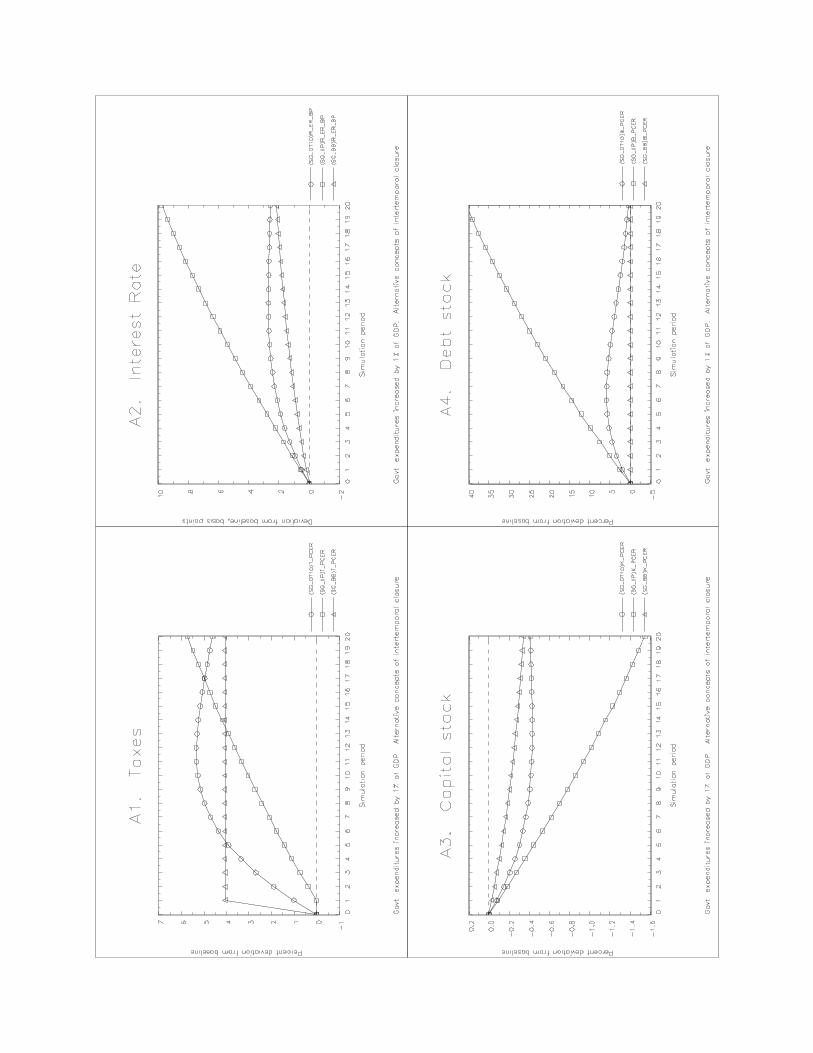
The qualitative differences among the debt targeting, IIP, and BB rules can be

easily grasped from examination of the set of charts labeled A. Each panel, pertaining to

one of the endogenous variables, has an analogous format. The DT10 simulation path is

identified by circles, the IIP path with squares, and the BB path with triangles.

20

Tax revenues for the first 20 periods are plotted in panel A1. The tax rate and tax

revenues must rise immediately under the BB rule. Increases in the tax rate and tax

revenues start to rise promptly under debt-stock targeting but do so only gradually; by the

6th period, tax revenues must rise further than under BB. Under the IIP rule, the tax rate

and tax revenues rise only sluggishly, and ultimately have to increase much more than in

the DT10 and BB simulations. The differences in fiscal rules lead to quite different paths

for the stock of debt (panel A4) and the interest rate (A2). Debt and the interest rate must

rise much higher relative to baseline under the IIP rule than in the other two cases. Note

that the debt stock cannot differ from baseline at all under the BB policy.

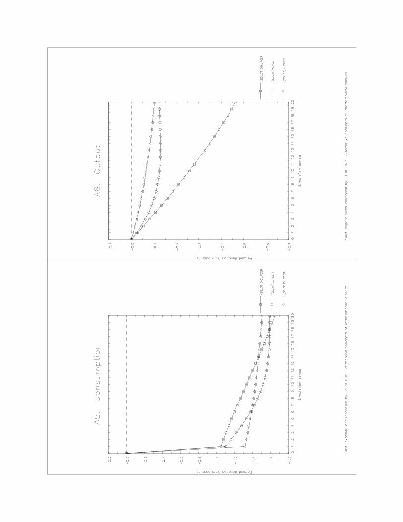
As expected from the analysis in sections II and III, the capital stock (A3) falls

least under the BB rule and considerably more under the IIP rule than in either of the

other two simulations. The different outcomes for the capital stock in turn cause

significantly different effects on output and consumption. Because of the simplified

nature of the model with its forward-looking specification of human wealth, consumption

falls immediately under all three fiscal regimes. The initial fall is smallest under IIP and

largest under BB. As time passes, however, the ranking of the effects on consumption is

reversed.

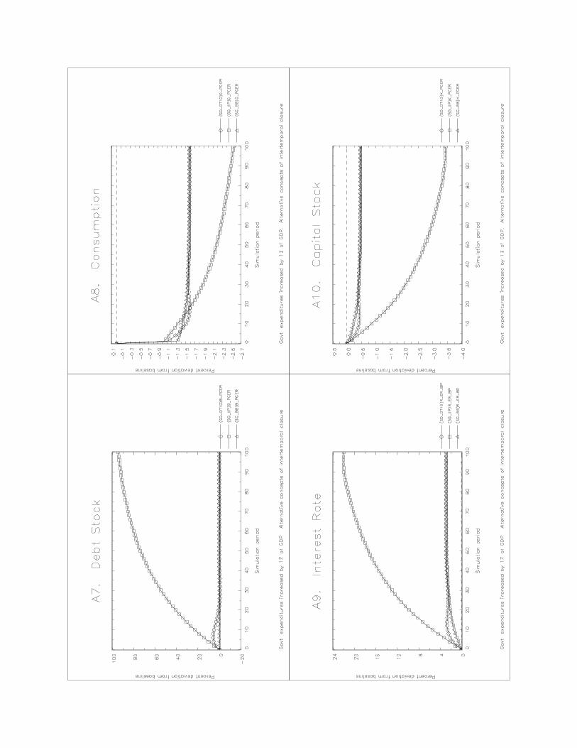
The relative differences over the longer run between the DT and BB rules on the

one hand and the IIP rule on the other are highlighted in panels A7 through A10. These

plots show the same three curves as before for the debt stock, consumption, the interest

rate, and the capital stock but now the horizontal axis is extended to 100 periods. The

variables in the DT10 and BB simulations are settling down to their new steady-state

paths after only some 20-30 periods. Under the IIP rule, the variables are not yet at their

new steady-state values after even 100 periods!

Seen from one perspective, the absolute magnitudes of the effects on the model’s

variables, especially on output, are not very large in any of the three simulations DT10,

BB, and IIP. These small absolute magnitudes are due to the simplified nature of the

21

In this neoclassical model, capacity utilization is always at 100 percent and thus output17

is entirely determined by the capital stock. With (n+8) not very large, an increase in publicspending leads to a nearly one-for-one crowding-out of private consumption, leaving not muchchange in output.

model. Differences in the relative magnitudes of the effects, however, are enormous. 17

For example, the long-run declines in the capital stock and output are more than 8 times

as large under the IIP rule as under the DT and BB rules. The debt stock must eventually

rise more than 200 percent above baseline under the IIP rule. Under either the DT or BB

rules, of course, the long-run value of the debt stock cannot deviate at all from baseline.

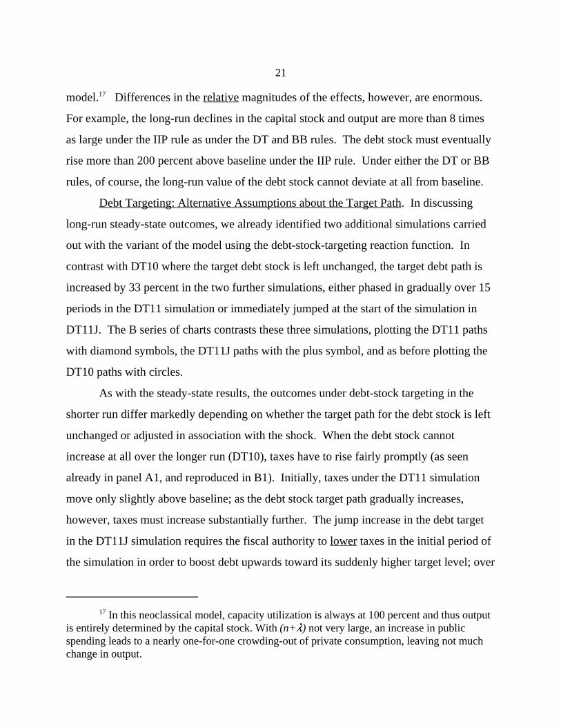
Debt Targeting: Alternative Assumptions about the Target Path. In discussing

long-run steady-state outcomes, we already identified two additional simulations carried

out with the variant of the model using the debt-stock-targeting reaction function. In

contrast with DT10 where the target debt stock is left unchanged, the target debt path is

increased by 33 percent in the two further simulations, either phased in gradually over 15

periods in the DT11 simulation or immediately jumped at the start of the simulation in

DT11J. The B series of charts contrasts these three simulations, plotting the DT11 paths

with diamond symbols, the DT11J paths with the plus symbol, and as before plotting the

DT10 paths with circles.

As with the steady-state results, the outcomes under debt-stock targeting in the

shorter run differ markedly depending on whether the target path for the debt stock is left

unchanged or adjusted in association with the shock. When the debt stock cannot

increase at all over the longer run (DT10), taxes have to rise fairly promptly (as seen

already in panel A1, and reproduced in B1). Initially, taxes under the DT11 simulation

move only slightly above baseline; as the debt stock target path gradually increases,

however, taxes must increase substantially further. The jump increase in the debt target

in the DT11J simulation requires the fiscal authority to lower taxes in the initial period of

the simulation in order to boost debt upwards toward its suddenly higher target level; over

22

the medium run, of course, taxes then have to rise sharply to prevent the debt stock from

increasing well above its new higher target level. The differing behaviors of the actual

stock of debt are shown in panel B4.

The interest rate (panel B2) must rise significantly higher and the capital stock

(B3) must fall further when the debt stock is targeted to rise above baseline. (The

ultimate rise in the interest rate and ultimate fall in the capital stock are eventually the

same under the DT11 and DT11J assumptions, of course.) Interest rates in the shorter run

rise even more under DT11J than under DT11.

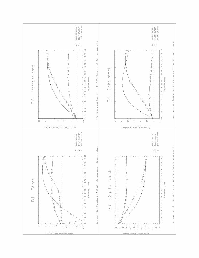
Output (B6) drops the least under the DT10 rule, drops significantly further under

DT11J when the target path for debt is immediately jumped to its higher level, and drops

the most under DT11 when the debt target path rises in gradual increments to its higher

level; differences between the three simulations increase with the passage of time. The

qualitative behavior of consumption (B5) is different; it initially falls furthest under DT10

and least far under DT11J; after fourteen periods, however, the decline in consumption

under DT11J exceeds that for both DT10 and DT11.

Shutting Off the Debt-Targeting Reaction Function for a Transitory Period. To

highlight another important dimension of intertemporal fiscal closure rules, we now

contrast the same DT10 simulation as before with yet two more debt-targeting

simulations, labeled DT10X and DT10Z. The DT10X and DT10Z variants are identical

to DT10 (with the target path for debt kept unchanged from baseline), except for the

critical difference that the operation of the debt-targeting reaction function is shut off

altogether for a 10-period interval at the start of the simulations. The function is shut off

by setting the DELAY term (see Figure B-1) to a value of zero in periods 1 through 10. t

The DT10X and DT10Z simulations thus illustrate in a crude way the "shock-absorption"

behavior in which policymakers may initially wait and see what happens following a

shock before acting to satisfy the intertemporal budget constraint or, alternatively,

"policy-delinquency" behavior in which policymakers initially ignore the intertemporal

23

See the discussion in section III of Bryant and Zhang (1996a).18

budget constraint and only remedy their delinquency in some subsequent period when

forced to do so by external forces (for example, by a bond-market crisis). In the18

DT10X simulation, the DELAY term rises gradually from a value of zero in the 10tht

period to a value of unity in the 20th period (in equal increments each period), which

value it maintains thereafter. The DT10Z simulation jumps the DELAY term from zerot

in period 10 immediately to the value of unity in period 11 and thereafter.

Because the DT10, DT10X, DT10Z, and BB simulations all have the same long-

run steady-state value for the target debt stock (unchanged from baseline), the four

simulations eventually generate the same steady-state values for all the model's variables.

The short-run and medium-run dynamic paths, however, are of course dramatically

different. The differences between the DT10, DT10X, and DT10Z simulations can be

studied in the panels of the C series of charts.

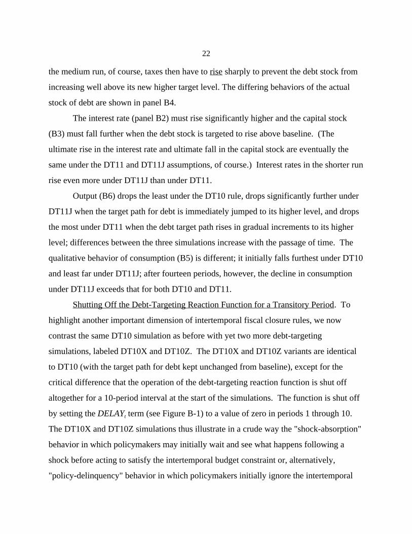
If the fiscal authority permanently raises government spending but aborts for the

first ten periods the implementation of the debt-targeting fiscal rule, taxes are not raised

in the initial periods; indeed, because of small declines in output and incomes, taxes

decline very slightly below baseline (C1). Once the tax rule is permitted to go to work in

the 11th period, however, taxes must then be vigorously raised (well above the increase in

taxes required under DT10). The required increase in taxes is particularly sharp when the

reaction function is suddenly turned on with full force (DT10Z).

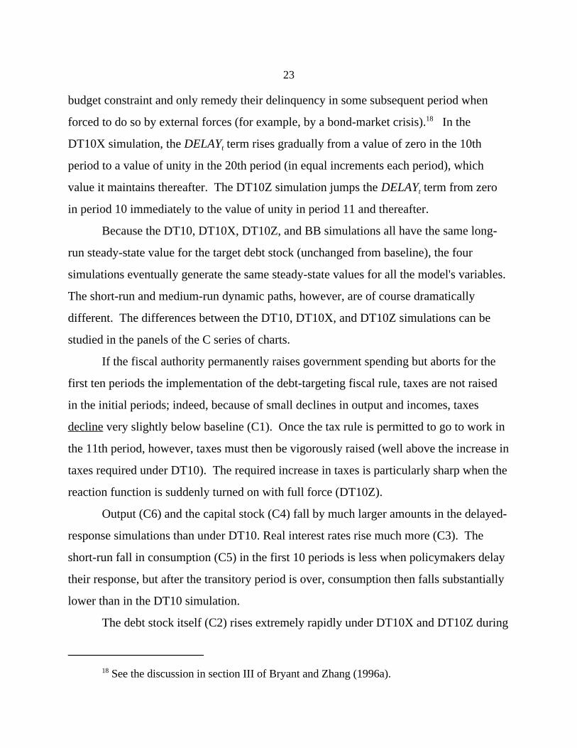
Output (C6) and the capital stock (C4) fall by much larger amounts in the delayed-

response simulations than under DT10. Real interest rates rise much more (C3). The

short-run fall in consumption (C5) in the first 10 periods is less when policymakers delay

their response, but after the transitory period is over, consumption then falls substantially

lower than in the DT10 simulation.

The debt stock itself (C2) rises extremely rapidly under DT10X and DT10Z during

24

the interim period when the reaction function is shut off. Then subsequently the debt

stock has to fall back sharply. Indeed, the debt stock eventually overshoots the baseline

path. The volatility in the debt stock, in the interest rate, and taxes is especially severe for

the case, DT10X, in which the reaction function is turned on incrementally between the

11th and 20th periods.

Choice of Feedback Parameters in the Fiscal Rule. The values of the feedback

coefficients to be used in a fiscal or monetary reaction function is a topic that has

received almost no systematic attention in previous research. Our own work so far leads

us to believe that the values of these coefficients can strongly influence the dynamic

behavior of a model system, sometimes in unwanted or implausible ways. As a first

demonstration of this point, we report here several further simulations using the debt-

stock targeting rule as an example. The differences among the simulations is due only to

different values of the feedback coefficients.

As pointed out in Bryant and Zhang (1996a), a debt-stock targeting rule which

includes only a proportional term but no derivative term can lead to an overshooting of

the debt-stock target and thus cause cyclical fluctuations in the dynamic economic

system. These cyclical fluctuations can be damped or eliminated with the introduction of

a derivative term and by varying the absolute and relative sizes of the feedback

coefficients.

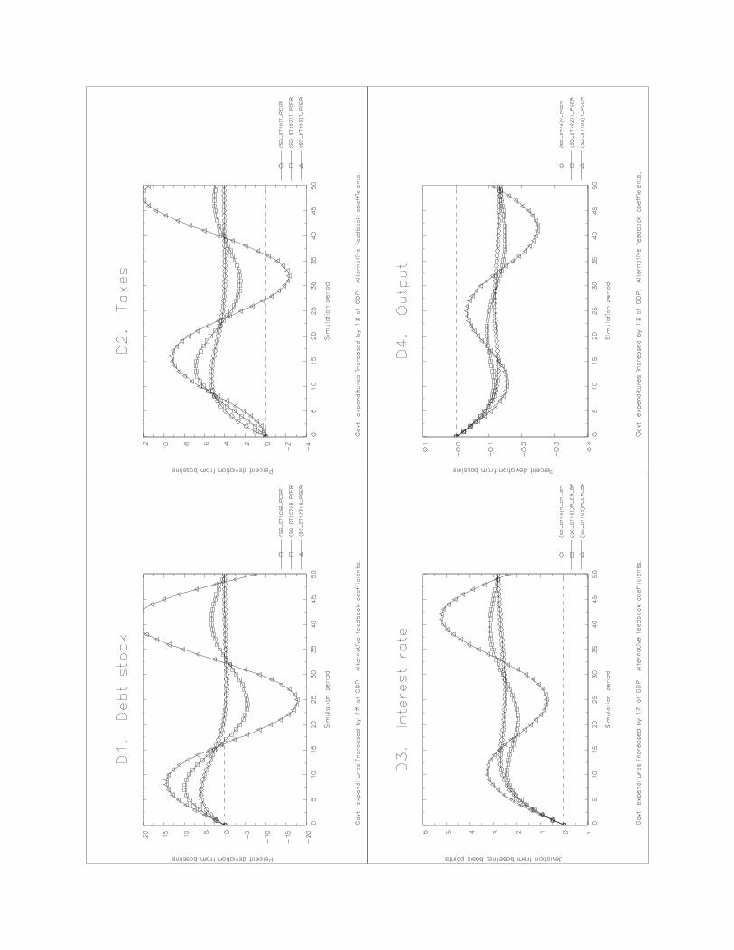
In the D set of charts that follows, as a benchmark we again use the DT10

simulation featured in the earlier comparisons. The feedback coefficients for this case

have the values " = .04 and " = 0.30. We continue to show the paths for this simulation1 2

with circle symbols. Two further simulations, DT102 and DT103, have the same value of

0.04 for the proportional coefficient " but use two alternative values for the derivative-1

term coefficient " . For DT102, " is set at 0.10 (one third the value of the coefficient in2 2

DT10); paths from DT102 are plotted with the square symbol. For DT103, the value of

" is lowered all the way to zero, so that the derivative term is eliminated altogether from2

25

In the standard version of full MULTIMOD, the reaction function for monetary policy -19

- a form of money targeting -- contains only a proportional term. From our experiments, we have

the debt-targeting reaction function; the triangle symbol is used to label the DT103 paths.

With no derivative term in the debt targeting rule, a permanent government

spending increase leads to large overshooting and then subsequently undershooting in the

debt stock and in tax collections (panels D1 and D2). These oscillations in turn generate

secondary cyclical fluctuations in the rest of the DT103 dynamic system, for example in

interest rates (D3) and output (D4). When a derivative term with moderate size of

feedback coefficient is added to the debt-targeting rule (DT102), the secondary cyclical

fluctuations are dampened considerably. In the benchmark case DT10, with a fairly large

value for the derivative feedback coefficient, the secondary fluctuations in the dynamic

system are virtually eliminated.

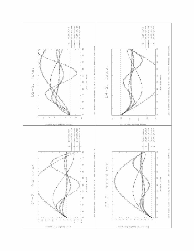
The sensitivity of the simulations to alternative assumptions is dramatized further

in the last set of charts (labeled D1a, D2a, etc.). Here we repeat exactly the same DT10,

DT102, and DT103 curves shown before but superimpose two further simulations. In the

DT104 simulation, we reduce both the proportional and derivative coefficients, thereby

damping the extent to which the rule requires the debt stock to move toward its target

path; the coefficient values are " = .01 (one fourth its size in the benchmark DT10 case)1

and " = 0.10 (one third the size in the DT10 case). The DT105 simulation makes the2

feedback coefficients still smaller: " = .005 and " = 0.05. As both sets of feedback1 2

coefficients are made small, the debt stock is permitted to move much further away from

the target path (D1a) and the other variables begin to oscillate with long cycles in a

clearly unstable manner (D2a, D3a, and D4a).

Our examples here use the debt-targeting rule for fiscal policy. We know from

other work, on the two-region model described in Bryant and Zhang (1996c) and on full

MULTIMOD, that analogous conclusions apply, with at least as much force, to the values

of the feedback coefficients in the reaction function for monetary policy.19

26

shown that the addition of a derivative term in the monetary-policy reaction function can damp oreliminate some puzzling secondary cycles that are present in standard simulations with fullMULTIMOD.

V. Concluding Remark

As foreshadowed in the general discussion in Bryant and Zhang (1996a), we have

illustrated here that the consequences of shocks or policy actions can be significantly

conditioned by the choice of intertemporal fiscal reaction function imposed on a

macroeconomic model. Significant variation can occur for different types of rule, for

alternative assumptions about the timing of a rule’s activation, and for alternative values

of the rule’s feedback coefficients. These points emerge clearly, as we have shown, even

with a model as simplified as the illustrative growth model used here. In Bryant and

Zhang (1996c), we illustrate and amplify the points with a more complex model, a two-

region abridgement of the IMF Staff’s MULTIMOD.

Appendix TableShort, Medium, and Long-Run Effects of a One-Percent-of-GNP Permanent Increase in Government Spending

Endogenousvariable Simulation Long-run(Units) label Period 1 Period 2 Period 3 Period 6 Period 15 steady state

Consumption DT10 -1.10 -1.16 -1.22 -1.38 -1.58 -1.59 (%) IIP -1.05 -1.08 -1.10 -1.20 -1.50 -2.66

BB -1.32 -1.33 -1.35 -0.01 -1.47 -1.59DT11 -0.97 -0.99 -1.03 -1.15 -1.66 -1.93DT11J -0.53 -0.66 -0.80 -1.19 -1.83 -1.93DT10X -1.05 -1.07 -1.09 -1.14 -1.58 -1.59DT10Z -1.06 -1.09 -1.11 -1.17 -1.79 -1.59

Output DT10 -0.02 -0.04 -0.06 -0.10 -0.13 -0.14 (%) IIP -0.03 -0.05 -0.08 -0.16 -0.37 -1.16

BB -0.01 -0.02 -0.02 -0.04 -0.09 -0.14DT11 -0.03 -0.07 -0.10 -0.20 -0.41 -0.47DT11J -0.06 -0.12 -0.17 -0.30 -0.44 -0.47DT10X -0.03 -0.05 -0.82 -0.17 -0.45 -0.14DT10Z -0.03 -0.05 -0.08 -0.16 -0.33 -0.14

Interest rate DT10 0.49 0.92 1.29 2.11 2.68 2.9 () , basis pts.) IIP 0.56 1.12 1.68 3.33 7.76 24.7

BB 0.18 0.34 0.50 0.92 1.81 2.9DT11 0.67 1.36 2.05 4.08 8.66 9.9DT11J 1.30 2.50 3.60 6.20 9.14 9.9DT10X 0.56 1.13 1.71 3.57 9.53 2.9DT10Z 0.54 1.09 1.63 3.34 6.91 2.9

Capital stock DT10 -0.08 -0.15 -0.21 -0.34 -0.43 -0.46 (%) IIP -0.09 -0.18 -0.27 -0.53 -1.23 -3.83

BB -0.03 -0.05 -0.08 -0.15 -0.29 -0.46DT11 -0.11 -0.22 -0.33 -0.65 -1.37 -1.56DT11J -0.21 -0.40 -0.57 -0.98 -1.44 -1.56DT10X -0.09 -0.18 -0.27 -0.57 -1.50 -0.46DT10Z -0.09 -0.17 -0.26 -0.53 -1.09 -0.46

Human wealth DT10 -2.27 -2.48 -2.65 -2.99 -2.96 -2.70 (%) IIP -2.22 -2.44 -2.66 -3.31 -5.07 -12.03

BB -2.54 -2.55 -2.56 -2.58 -2.63 -2.70DT11 -2.06 -2.31 -2.58 -3.54 -6.28 -5.72DT11J -1.87 -2.85 -3.71 -5.59 -6.70 -5.72DT10X -2.22 -2.46 -2.71 -3.57 -7.18 -2.70DT10Z -2.24 -2.50 -2.76 -3.67 -6.08 -2.70

Government debt DT10 1.93 3.42 4.51 5.89 2.44 0 (%) IIP 2.57 5.07 7.51 14.48 32.46 202.7

BB 0 0 0 0 0 0DT11 2.70 5.63 8.76 18.86 42.83 33.3DT11J 10.33 19.24 26.77 41.73 44.38 33.3DT10X 2.59 5.37 8.35 18.67 54.70 0.00DT10Z 2.59 5.37 8.35 18.64 35.87 0.00

Tax revenues DT10 1.01 1.91 2.69 4.35 5.17 4.08 (%) IIP 0.01 0.38 0.74 1.77 4.47 15.22

BB 4.04 4.04 4.05 4.05 4.07 4.08DT11 -0.19 -0.28 -0.27 0.24 7.13 7.62DT11J -12.19 -8.90 -5.78 2.01 10.76 7.62DT10X -0.03 -0.05 -0.08 -0.17 6.62 4.09DT10Z -0.03 -0.05 -0.08 -0.16 11.66 4.09

Tax rate DT10 26 48 68 110 131 105 () , basis pts.) IIP 1 11 20 48 120 377

BB 100 101 101 101 103 105DT11 -4 -5 -4 11 188 200DT11J -300 -218 -139 57 278 200DT10X 0 0 0 0 176 105DT10Z 0 0 0 0 298 105

__________________________Variables are measured in real terms per effective labor unit (except the interest rate and tax rate); see text.

%: deviation of the simulation values from baseline values, measured in percentage points.

): absolute deviation of the simulation values from baseline values, measured in basis points (e.g., a change in the interest rate from 5.50 percent to5.65 percent would be reported as 15.0 basis points; a change in the tax rate from .24 to .26 would be reported as 200 basis points.

Brief description of simulations (see text for detailed description):DT10: Debt-stock targeting rule with no change in the target path for debt.IIP: Incremental interest payments rule.BB: Balanced budget rule.DT11: Debt stock targeting rule, with target path gradually increased by 33 percent.DT11J: Debt stock targeting rule, with target path jumped immediately by 33 percent.DT10X: Debt-stock targeting rule with no change in the target path for debt; delayed implementation for 10 years, with phased in implementation thereafter.DT10Z: Debt-stock targeting rule with no change in the target path for debt; delayed implementation for 10 years, with immediate implementation thereafter.

27

REFERENCES

Barro, Robert J., and Xavier Sala-I-Martin. 1995. Economic Growth. (McGraw-HillAdvanced Series in Economics.) New York: McGraw-Hill, 1995.

Blanchard, Olivier J. 1985. "Debt, Deficits, and Finite Horizons." Journal of PoliticalEconomy 93: 223-47.

Bryant, Ralph C., and Long Zhang. 1996a. “Intertemporal Fiscal Policy inMacroeconomic Models: Introduction and Major Alternatives.” BrookingsDiscussion Paper in International Economics No. 123, June 1996.

Bryant, Ralph C., and Long Zhang. 1996b. “Alternative Specifications of IntertemporalFiscal Policy in a Small Theoretical Model." Brookings Discussion Paper inInternational Economics No. 124, June 1996.

Bryant, Ralph C., and Long Zhang. 1996c. “Intertemporal Fiscal Policy in a Two-Region Abridgement of MULTIMOD." Forthcoming as a Brookings DiscussionPaper in International Economics, 1996.

Buiter, Willem H. 1988. "Death, Birth, Productivity Growth and Debt Neutrality."Economic Journal 98 (June 1988): 279-93.

Weil, Philippe. 1989. "Overlapping Families of Infinitely-lived Agents." Journal ofPublic Economics 38: 183-98.

Yaari, Menahem E. 1965. "Uncertain Lifetime, Life Insurance, and the Theory of theConsumer," Review of Economic Studies, Vol. 32 (April 1965), pp. 137-50.

Zhang, Long. 1996. Intertemporal Fiscal Closure Rules and Fiscal Policy in aContinuous OLG Model. Doctoral Dissertation, Department of Economics,University of California, Santa Cruz.