Fiscal Decentralization with a Redistribution Rule vs

Sosyoekonomi RESEARCH

ARTICLE

ISSN: 1305-5577

DOI: 10.17233/sosyoekonomi.2020.02.06

Date Submitted: 08.03.2019

Date Revised: 11.02.2020

Date Accepted: 21.02.2020 2020, Vol. 28(44), 107-136

Fiscal Decentralization with a Redistribution Rule vs. Fiscal Centralization

Zeynep Burcu BULUT-ÇEVİK (https://orcid.org/0000-0002-3318-1122), Department of Public Finance,

Ankara Yıldırım Beyazıt University, Turkey; e-mail: [email protected]

Mali Merkezîleşme ile Yeniden Dağıtım Kuralı altında Mali Yerelleşmenin

Karşılaştırılması

Abstract

This paper compares the case of fiscal decentralization (FD) with an intergovernmental transfer

rule to the case of fiscal centralization (FC) from a theoretical perspective while focusing on Markov-

perfect Nash equilibrium by a continuum of citizens, local governments and a central government,

which interact strategically. Simulation analysis shows that both the degree of spillovers and capital

mobility play a role in the comparison of these two cases. In the presence of spillovers, the welfare of

FD case is higher than the one of FC which is an unexpected result but points out the positive effect of

a redistribution rule in FD model in terms of welfare. On the other hand, the growth rate of FD is lower

than the FC case when there are spillovers. So, fiscal discipline, provided by the redistribution rule,

prevents inefficiently low tax rates which pull down the growth rate. In addition, when spillovers are

not allowed, capital mobility determines which case is superior.

Keywords : Fiscal Decentralization, Fiscal Centralization, Intergovernmental

Transfer/ Redistribution Rule, Welfare, Capital Mobility.

JEL Classification Codes : H77, H23, O41, C63, C72.

Öz

Bu çalışma, yönetimlerarası transfer kuralına sahip mali yerelleşme ile mali merkezîleşmenin

teorik perspektiften karşılaştırmasını yapmaktadır. Vatandaşların, yerel yönetimlerin ve merkezi

hükümetin stratejik olarak etkileşimde olduğu bu modelde Markov-perfect Nash dengesi üzerinde

çalışılmıştır. Simülasyon analizleri, yayılma (spillovers) derecesinin ve sermaye hareketliliğinin bu

karşılaştırmada etkili olduğunu göstermiştir. Yayılmanın olduğu durumda, mali yerelleşmede görülen

refah seviyesinin mali merkezîleşmeden yüksek olduğu görülmüştür. Bu durum beklenmeyen bir

sonuç olmasına karşın, transfer kuralının mali yerelleşmeye refah açısından olumlu etkisine işaret

etmektedir. Diğer yandan, yayılmanın olması halinde, mali yerelleşme durumunda büyümenin mali

merkezîleşmeden düşük olduğu gözlenmiştir. Bu durum, transfer kuralı ile ortaya konan mali

disiplinde hedeflenen vergi oranının, çok altına düşememesi sebebiyle büyümenin de yükselmesinin

engellendiği sonucuna varılabilir. Yayılmanın olmaması durumunda ise, durumların birbiri üzerindeki

üstünlüğünü belirleyenin sermaye hareketliliği olduğu bulunmuştur.

Anahtar Sözcükler : Mali Yerelleşme, Mali Merkezîleşme, Yönetimlerarası Transfer/

Yeniden Dağıtım Kuralı, Refah, Sermaye Hareketliliği.

Bulut-Çevik, Z.B. (2020), “Fiscal Decentralization with a Redistribution

Rule vs. Fiscal Centralization”, Sosyoekonomi, Vol. 28(44), 107-136.

108

1. Introduction

Fiscal decentralization (FD) refers to “the devolution of fiscal powers from national

government to subnational governments”. The necessity of introducing FD comes from

facilitating the fiscal duties of the government, which is assumed to conclude with the

efficient allocation of resources. Although the logic of the FD is firstly introduced to the

literature by Tiebout (1956), extensive research about FD has conducted along with the

seminal work of Oates (1972). This work focuses largely on the economic effects of FD and

reasons behind the tendency to FD among developed countries by comparing centralized

and decentralized fiscal systems.

There is a wide literature discussing the advantages and disadvantages of FD and

fiscal centralization (FC) both theoretically and empirically. The motivation of the most

empirical studies arises with the tendency towards FD among developed countries, so that

they focus on whether there exists a relationship between growth and FD. On the other hand,

theoretical studies investigate not only growth but also welfare effects of FD from different

perspectives. One perspective is related to the political economy point of view1. For instance,

Besley and Coate (2003) compare decentralized and centralized fiscal systems through this

perspective. They show the existence of a threshold level of public good spillovers with

different choices of legislature where FD or FC yields higher welfare level than the other

one. The other perspective is investigating the welfare consequences of tax competition and

tax coordination (or harmonization) among localities, states or countries2. Arguments about

the economic effect of tax competition to the economy have been widely discussed and not

reached an agreed decision yet, but most of the studies in this literature argue that inefficient

level of public good provision is observed due to low levels of the tax rate. (Bradford and

Oates, 1971; Oates, 1972; Rohac, 2006; Brueckner, 2003). In this paper, we include tax

competition in our model with some political economy-related variables to be the part of

these discussions while our research question is investigating the growth and welfare

comparisons for the cases of FD and FC with some specific properties3.

One of the properties in our model is to include intergovernmental transfers into the

FD model. Some studies related to decentralized fiscal systems highlight the importance of

intergovernmental fiscal systems. The necessities of intergovernmental transfers emerge

from vertical and horizontal fiscal imbalances. These fiscal imbalances occur due to the

mismatch of local government expenditure and revenue and in order to remove these,

intergovernmental transfers are widely used by the governments. Although they are widely

preferred, they may cause some problems such as moral hazard problem since local

governments identify them as an insurance against their poor decisions, which creates moral

1 See Lockwood (2006) for a review. 2 Razin and Sadki (1991); Zodrow (2003); Keen (1993). 3 These properties are discussed in the model part in detail.



109

hazard problem. Fiscal indiscipline can be counted as another problem in distributing

transfers due to common pool problem, soft financing and grant design (Eyraud & Lusinyan,

2011). Hence designing a transfer mechanism or rule4 should be crucial to make it effective.

Ma (1997) and Shah (1995) claim that effective intergovernmental transfers should have

some specific properties such as: revenue adequacy, local tax effort, equity, transparency

and stability. However, in most of the theoretical models, other than lump sum transfers,

intergovernmental transfer rules or mechanisms, which have some of these properties, are

omitted. On the other hand, in particular, Akin et al. (2016) proposes a linear redistribution

rule, which aim to correct for the income and tax collection effort differences among

jurisdictions, in a static model. Their objective is to observe the effect of FD with a

predetermined transfer rule on fiscal discipline compared to the effect of FC. They find that

FD with the transfer rule positively affects the fiscal discipline, but income distribution

worsens compared to the centralized system. This study also uses this linear transfer rule

with a slight difference; instead of tax collection effort, used to represent efficiency property,

we introduce tax revenue and tax revenue target for each locality. This change does not affect

the fact that it still represents the efficiency property, since it also shows how much tax

revenue is collected compared to the target for that locality as in the case of measuring the

tax collection effort deviation.

Another debated topic in FD literature is the utility structure of local governments.

Local governments, which maximize the local welfare of its citizens, are called ‘Pigouvian’

governments. (Zodrow & Mieszkowski, 1986) On the other hand, Brennan and Buchanan

(1980) define governments as pure rent-seekers, who provide public goods with the

expectation to collect rents for themselves and call them ‘Leviathan’ governments. Edwards

and Keen (1996) find that if governments are not fully self-serving, but partly benevolent

then desirable levels of policy variables are observed. Rauscher (1998) also uses this kind

of government (neither fully benevolent nor fully self-caring) in his studies to show that

inter-jurisdictional competition for mobile factors of production forces the government to

raise the efficiency of the public sector. In addition, Epple and Nechyba (2004) compare

these two extreme models of local government behavior from local tax rates and public good

levels and conclude that both not fully selfish and not fully benevolent government gives

desired levels of tax rate and public good simultaneously. This study takes into account these

discussions and introduces political economy variables, rent-seeking variable and degree of

selfishness of the local government5, into the utility form of the government. This utility

form allows the local governments to be fully benevolent, fully selfish or between these two.

This paper extends the literature as follows. In fiscally decentralized theoretical

models, transfer rule or mechanism is mostly missing, other than lump-sum transfers as

4 Transfer rule, intergovernmental transfer rule and redistribution rule represent the same idea and so are used

interchangeably throughout this study. 5 Rent seeking variable is denoted as ′𝑅′ and selfishness of the politician as ‘L’ in the paper and will be explained

in detail in the model section.



110

stated before, where Ma (1997) and Shah (1995) argue insufficiency of lump-sum transfers

in observing the effects of FD on the economy and highlight the significance of a well-

designed redistribution rule. This study tries to fill this gap by focusing on how the inclusion

of a linear transfer rule affects the comparison of fiscally decentralized and centralized

systems from a theoretical perspective. To be able to use a transfer mechanism as a linear

constraint in our government’s problem, this study includes equity and local tax effort, in

the name of efficiency, properties in decentralized fiscal case. Secondly, most of the

theoretical FD models do not include central government but only local governments since

in decentralized fiscal systems, the main fiscal decision makers are the local governments.

However, even in the most decentralized fiscal systems such as US, Canada, etc., central

government detects and controls the actions of local governments and if necessary, it takes

actions in order to maintain the stability, equity or efficiency of the overall economy. This

study does not ignore this argument and incorporates a central government, which controls

local governments through a redistribution rule, where local governments are the main fiscal

executives in the case of FD of this study. Hence, there will be a 3-stage game in the

decentralized fiscal system.

The present paper is designed to investigate and compare the growth and welfare

effects of FD and FC. The model has some similarities with the Chu and Yang’s (2012)

endogenous growth model as well as the redistribution system that was firstly constructed

by Akin et al. (2016) in the literature. The model of Chu and Yang (2012) can be considered

as an extension of Besley and Coate’s (2003) public provision model. In Besley and Coate’s

model, the public good provision model is in the static form without tax competition as well

as the model of Akin et al. (2016). The model of Chu and Yang (2012) is a dynamic

endogenous growth model with the allowance of tax competition and public good spillovers.

They examine differences between FD and FC via this endogenous growth model. They

show the dominating effect of FD in growth over FC, but in welfare, the superiority depends

on capital mobility level. The main difference between their model and the current model is

the redistribution mechanism that Wilson (1999) claims as a necessary procedure if tax

competition exists in the model. In addition, the political economy point of view is limited

to interpreting the degree of rent-seeking variable with selfishness parameter.

In the decentralized case, local governments choose their policy independently,

simultaneously but non-cooperatively for each point in time t. There is a central government

that has no role in fiscal policy only determines the redistribution. Local governments cannot

internalize public good spillovers but there exists tax competition since each locality chooses

his own tax rate at each time t. After central government decides transfers, local governments

maximize their lifetime utility and then citizens maximize their own lifetime utility subject

to flow budget constraint. In the case of centralized system, there are local governments that

have no role in fiscal policy because they are assumed to coordinate each other and

symmetric. Local governments only get transfers from central government and use it for

local expenses. Since central government coordinates the fiscal policy and set a fixed tax

rate for all jurisdictions, the spillovers of public goods are internalized across jurisdictions.

In other words, there is no tax competition. After the central government decides on fiscal

policy, citizens maximize their own lifetime utility subject to flow budget constraint.



111

Analytical solutions can be found for both cases (FD and FC), however, because of

the complexity of the results, comparisons between decentralized and centralized cases need

simulation analysis. In welfare comparisons, the effects of spillovers and capital mobility

play significant roles. Most of the theoretical FD studies6 argue that FD provides higher

growth but lower welfare levels than FC, but in these studies, redistribution mechanism is

mentioned but omitted. So, introducing redistribution rule may lead to unexpected results

than these studies or than Decentralization Theorem. For instance, when there are spillovers

among governments, FD with redistribution rule provides higher welfare than FC even tax

rate is higher in case of FD than FC. So, lower tax rate in FC model means lower tax revenue,

which lessens the utility levels of citizens since the utility of citizens is composed of private

consumption, home public good and neighbor public good levels. However, this comparison

changes with respect to the level of capital mobility when there are no spillovers. In case of

low mobility, the decentralized case has a higher welfare level than the centralized case. On

the other hand, in case of high capital mobility, FC provides higher welfare than FD. These

findings show the corrective effect of a redistribution rule, which takes into account equity

and efficiency, in fiscally decentralized economies. In other words, fiscally decentralized

economies may avoid the disadvantages of being decentralized compared to being

centralized by introducing a linear redistribution rule, which has equity and efficiency

properties, according to the welfare level comparisons. Hence, the results of welfare

comparisons may seem so different from the Decentralization Theorem, however in

decentralization theorem, there is not intergovernmental transfer system which may affect

the whole theorem if included. This study shows how Decentralization Theorem may differ

when a linear transfer rule is introduced to the decentralized fiscal model.

Another result, related to growth rate comparisons, also depends on the existence of

spillovers. The growth rate in the decentralized case with redistribution rule is lower than

the rate in the centralized case when there are spillovers. So, with the existence of spillovers,

fiscal discipline, provided by the redistribution rule, prevents inefficiently low tax rates,

which pull down the growth rate.

The organization of this paper is as follows: Section 2 introduces the model then

Section 3 reports the results of the model. The final section, Section 4, provides the overall

summary and conclusions.

2. The Model

In our model, there are three agents, interacting with each other. These agents are

citizens, local governments, and a central government. Time is continuous. Tax competition

between local governments and public good spillovers across regions are allowed. In order

to reduce the complexity while providing endogenous growth, A-K type endogenous growth

6 Oates (1972,1999), Wilson (1999), Chu & Yang (2012).



112

model is preferred. We assume that capital is mobile, and its income is the only revenue

source for the government.

In this study, the differences between FD and FC are based on the authority of fiscal

policy. In FD, local governments are in charge of fiscal policy whereas, in FC, the central

government is the only authority. The main difference of this model than already existing

models in the literature is including a linear redistribution rule with tax competition and

public good spillovers to the FD case, and examining how different the results are than

Decentralization Theorem and which mechanism makes the difference.

In the decentralized fiscal set up, central government only distributes tax revenue,

which local government collects, according to a linear redistribution rule. With this transfer,

local governments (LGs) choose their policy independently, simultaneously but non-

cooperatively for each point in time t. Local governments cannot internalize public good

spillovers but there exists tax competition since each locality chooses his own tax rate at

each time t. After central government (CG) decides transfer amounts that each locality takes,

local governments maximize their lifetime utility and then citizens maximize their own

lifetime utility subject to flow budget constraint.

In the centralized set up, there are LGs but has no role in fiscal policy because they

are assumed to coordinate each other and symmetric. They only get transfers from CG and

use it for local expenses. Since CG coordinates the fiscal policy and set a fixed tax rate for

all jurisdictions, the spillovers of public goods are internalized across jurisdictions. (i.e. no

tax competition) After CG decides the fiscal policy, citizens maximize their own lifetime

utility subject to flow budget constraint.

After briefly explaining the FD and FC set ups in the preceding paragraphs, the agents

and their characteristics are explained in the coming subsections in detail.

2.1. Citizens

Citizens are identical, living in geographically distinct but symmetric districts. For

simplicity, two jurisdictions are assumed to exist: home and neighbor jurisdictions. Citizens7

typically maximize their utility subject to flow budget constraint. It is a dynamic model with

an allowance of public good spillovers. * is used to denote neighbor variables.

The lifetime utility of citizens in each jurisdiction is represented by

U = ∫ e−ρt[ln Ct + (1 − s) ln Gt + s ln Gt∗]dt

∞

0 (1)

7 Since citizens are representative agents, no subscripts or superscripts are used for citizens. Only jurisdiction

based superscript is used which is ‘*’.



113

where ρ > 0 is a discount factor, Ct is the level of consumption, Gt is the level of local public

goods in the home jurisdiction at time t and Gt∗ is the level of local public goods in the

neighbor jurisdiction at time t. 𝑠 ∈ [0,0.5] is the degree of positive spillovers: 𝑠 = 0 means

that the citizen only care about the public good provided in home jurisdiction. It is assumed

that the public good at neighbor jurisdiction cannot affect the citizen more than the public

good at home jurisdiction since the citizen is living in the home jurisdiction. In addition, the

public good at neighbor jurisdiction cannot affect the citizen’s well-being negatively since

the citizens are assumed to be rational, in other words, the citizen will prefer not to use the

neighbor’s public good at all, other than getting negative utility. The idea of this set-up is

similar with Besley and Coate’s (2003) public good provision model with the same range of

positive spillover degree.

In this model, agents are not allowed to move but capital is mobile and taxed, so tax

competition is observed under mobile capital. Due to the mobility of capital, there are

different levels of capital for two jurisdictions. The capital level distributed to the home

locality is denoted as 𝐷𝑡 , whereas the capital level distributed to the other neighbor locality

is denoted as 𝐹𝑡 so that the total amount of capital is 𝐾𝑡 = 𝐷𝑡 + 𝐹𝑡. The total amount of tax

paid by the citizen living in home jurisdiction to the government is 𝜏𝑡𝑖𝐷𝑡 + 𝜏𝑡∗𝑖∗𝐹𝑡 at time t.

The ratio of capital allocated to neighbor jurisdiction over total capital is denoted by 𝜃𝑡 =𝐹𝑡

𝐾𝑡⁄ so 1 − 𝜃𝑡 =

𝐷𝑡𝐾𝑡

⁄ is the ratio of capital allocated to the home jurisdiction over total

capital per citizen at time t.8 This construction leads to a constraint, which is:

𝜃𝑡 ∈ [0,1]

Citizens choose their saving and consumption amounts while aiming to maximize

their lifetime utility subject to flow budget constraint, which is9:

𝐾�� = (1 − 𝜏𝑡)𝑖𝐷𝑡 + (1 − 𝜏𝑡∗) 𝑖∗𝐹𝑡 − 𝐶𝑡 − 𝑀(𝜃𝑡 , 𝐾𝑡 , 𝑚) (2)

where Ct is the level of consumption, 𝐾𝑡 is the total capital level belonging to the citizen,

residing in home jurisdiction, 𝐷𝑡 is the capital level allocated to home jurisdiction and 𝐹𝑡 is

the capital level allocated to foreign jurisdiction. In addition, 𝜏𝑡 is the tax rate levied on each

unit of capital at home jurisdiction, 𝜏𝑡∗ is the tax rate levied on each unit of capital at

neighbor jurisdiction at time t and 𝑖 is the rental rate of return at home whereas 𝑖∗ is the

rental rate of return in neighbor jurisdiction.

8 The same equalities hold for the citizens, living in the neighbor jurisdiction. In other words, the capital level

distributed to the neighbor locality is denoted as 𝐷𝑡 ∗, whereas the capital level distributed to the home locality

is denoted as 𝐹𝑡 ∗ so that the total amount of capital is 𝐾𝑡

∗ = 𝐷𝑡∗ + 𝐹𝑡

∗. So, 𝐷𝑡 ∗ does not have to be equal to 𝐷𝑡.

9 Depreciation of the capital is widely introduced in growth models, however in order to reduce the complexity of

the model, depreciation of the capital is omitted in this study since it is out of the scope for this paper.



114

The last term in budget constraint is the cost of investing in neighbor jurisdiction

instead of home jurisdiction. It represents all the possible uncertainties and risks coming

with the investing abroad. The functional form is similar to the ones in the papers of Persson

and Tabellini (1992), Lejour and Verb (1997) and Chu and Yang (2012). The form of the

cost function is as follows:

𝑀(𝜃𝑡 , 𝐾𝑡 , 𝑚) = 𝐾𝑡(𝜃𝑡)2

𝑚⁄

where 𝑚 ∈ (0, ∞) is the degree of capital mobility. If 𝑚 = ∞, i.e. the capital is perfectly

mobile, then there will be no cost, however if 𝑚 = 0, i.e. the capital is perfectly immobile,

then the cost will go to infinity which means it is not rational to move the capital. As will be

shown in the coming section, the higher the degree of capital mobility, the lower the tax rate

is.10 Costly implementation of capital flight for citizens explains the increasing property of

cost function, whereas convexity property implies marginal cost increases as the size of

capital flight increases.

2.2. Firms

The owners of the firms are the households and each firm aims to maximize its profit

and chooses how much to produce. In other words, a firm solves the following problem:

max𝐾𝑡

𝜋 = 𝐹(𝐾𝑡) − 𝑖𝐾𝑡

Solution of the problem with A-K type production function is11

𝐹′(𝐾𝑡) = 𝑖 = 𝐴

So, the rental rate of the firm is equal to the technology level of the locality. Since

the localities are symmetric (i.e. they have similar properties such as technology level) and

firms in the neighbor jurisdiction also solve the same problem, the rental rate of each locality

will also be equal to each other:

𝑖 = 𝑖∗

10 Deveraux et al. (2008) find out loosening capital controls decrease the corporate tax rate in OECD countries

in 1980s and 1990s. Winner (2005) argues that capital mobility decreases the capital tax burdens in OECD

countries. 11 The profit coming from the firm is zero. Also, the reason behind the choice of AK type production function is

introducing endogenous growth to the model while having a tractable type of production function.



115

2.3. Governments

There are two types of government: LGs and CG, and the roles differ significantly

both in decentralized and centralized case. Because of these differences, governments will

be explained case by case.

2.3.1. Local Government (LG)

2.3.1.1. Decentralized Case

Brennan and Buchanan (1980) criticize ‘Pigouvian’ type governments and propose

‘Leviathan’ type governments. He declares that since politicians run governments,

governments are pure rent seekers. With this idea, policy-making governments may be fully

selfish or fully benevolent or between these two in this study. How the politicians are

selected or why is not this study’s concern so the political economy part is mostly missing.

However, allowing using some portion of the tax revenue for politician’s self-interested

purposes makes the governments not fully benevolent. (Lockwood, 2006) LG maximizes

his lifetime utility subject to the law of motion for capital and instantaneous balanced budget

constraint.

The lifetime utility is as follows:

𝑉 = (1 − 𝐿)(∫ e−ρt[ln Ct + (1 − s) ln Gt + s ln Gt∗]dt

∞

0) + 𝐿(∫ 𝑒−𝜌𝑡∞

0[ln 𝑅𝑡]) (3)

where 𝑈 is the lifetime utility of a citizen and 𝑅𝑡 is the amount of tax revenue that is used

for self interested purposes by politicians at time t. 𝐿 ∈ [0,1] is given exogenously12 which

represents the degree of selfishness of the politician, also known as rent seeking parameter

(Lockwood, 2006; Edwards and Keen, 1996: Rauscher, 1998). If 𝐿 = 0, the government

does not use any tax revenue for his self-interested purposes, so the government gets utility

only from the utility of citizens, i.e, the government is fully benevolent. If 𝐿 = 1, the

government does not care about the citizen’s utility, only cares about his own purposes, i.e.

the politician is fully selfish.

There is a balanced budget constraint, that should hold for each point in time, t. It is

as follows:

Gt + Rt = Nt (4)

where Nt is the amount of transfers sent by CG. The source of these transfers is tax revenue,

collected by LGs. The interpretation of this equation is that government use transfers either

12 The degree of the selfishness of the politician, L, can also be endogenously determined, however in that case

there will no benefit for this study’s research question but only complicates the model.



116

for the public good provision or for its own political concerns. The transfer amount is

decided with a rule by CG.

Given citizen’s best response, the LG chooses fiscal policy variables, which are tax

rate, rents, and public goods by maximizing lifetime utility of the politician (equation 3) with

respect to the law of motion for capital (equation 2) and budget constraint (equation 4).

2.3.1.2. Centralized Case

As stated before, in centralized case, CG is the main decision maker in fiscal policy

and LGs have no role. They only get the transfers from the CG and distribute it. In other

words, there is no choice or optimization problem for LGs in centralized case. There is only

one type of government, CG, in centralized case.

2.3.2. Central Government (CG)

2.3.2.1. Decentralized Case:

In this study, for simplicity, it is assumed to exist only two geographically distinct

but symmetric localities. And the objective function of CG is the utilities of these localities.

So CG maximizes lifetime utilities of both localities with respect to lifetime balanced budget

constraint. The objective function is as follows:

U + U∗ (5)

where U is the lifetime utility of a citizen and in the form of (1). U∗ is the lifetime utility of

the other locality’s citizen with the same form.

Assume there is a common pool, that all the localities drop their tax revenue into that

pool and there exists a superior unit, which is central government. It decides which locality

should get how much tax revenue from that pool. CG is assumed to be fully benevolent. This

common pool can be represented as13:

AτtKt + Aτt∗Kt

∗ = Nt + Nt∗ (6)

CG does not directly decide the transfer amounts since there is a redistribution rule.

In the literature, the transfer mechanism is known as balancing tool between

government entities. In this study, the redistribution rule is similar to Akin et.al. (2016),

however there exists a slight difference. Akin et.al. (2016) focus on tax collection effort, but

13 From the firm problem, it is known that the rental rate of a locality is equal to the technology level and due to

symmetricity of localities, technology levels and rental rates of localities are both equal to each other. With this

knowledge, the left-hand side of the equation (6) is derived.



117

in this study tax revenue levels and targets are defined and used. In this rule, there are two

basic parts: efficiency and equity. Efficiency part aims the fiscal discipline by targeting the

tax revenue. Equity part aims to destroy the horizontal imbalances between localities.

Nt = p[τtKt − Tt] + φ[Yt − AKt] (7)

where p is the punishment parameter and γ is the income compensation parameter, Tt is the

tax revenue target level and Yt is the income target level that are set exogenously. For

instance, if a locality cannot reach tax revenue target level then CG punishes the locality and

decreases the transfer amount with a degree of p. Also, if a locality cannot reach the income

target level then CG increases the transfer amount with a degree of γ in order to decrease the

horizontal imbalances.

The former part, p[τtKt − Tt], is the efficiency part since unless locality can collect

its potential amount of tax revenue, it is punished with decreasing transfers. In other words,

efficiency part provides the fiscal discipline by targeting the tax revenue level. The latter

part, φ[Yt − AKt], is the equity part since the aim of this equation is equalization among

localities in terms of their income levels. In other words, equity part decreases the horizontal

imbalances between localities.

For the current case, CG is not involved in fiscal policy decisions, its role is only

determining the parameter values in redistribution rule, so that, it decides the amounts of the

transfers indirectly. Hence, CG maximizes (5) subject to (6) and (7) to determine p and γ.

2.3.2.2. Centralized Case

The problem of CG is similar to the problem of LG in decentralized case since the

fiscal policy decision maker is CG in centralized case and it is LG in decentralized case. The

main difference between them is the (non) existence of redistribution rule. In centralized

fiscal system, CG makes its decisions according to the total level of tax revenue; however,

LG in decentralized case uses a portion of total tax revenue, which is decided by the

redistribution rule.

Hence, the balanced budget constraint for CG will be as follows:

Gt + Rt = AτtKt

whereas the lifetime utility form is similar to the equation (1) with a few differences:

U = ∫ e−ρt[ln Ct + ln Gt]dt∞

0

In centralized case, there are no different tax rate or interest rate between localities,

so law of motion of capital in equation 2 becomes as follows:

Efficiency Equity



118

𝐾�� = (1 − 𝜏𝑡)𝑖𝐾𝑡 − 𝐶𝑡

2.4. Fiscal Centralization and Fiscal Decentralization

This study does not focus on optimal taxation policy but comparing two different

fiscal systems. Ramsey type approach is assumed in the timing of events. So, under full

commitment, governments move first and then given the policy decisions, citizens determine

their consumption and saving levels. Contrary to the optimal fiscal policy literature of

Ramsey problems, this study is not interested in the comparison of primary and dual

approaches in Ramsey problem or choosing one to another. This study aims to answer which

type of countries can benefit from decentralization or centralization by looking at the

parameter values of the model results. Also, how the results differ from the usual findings

when a redistribution rule is included into the model.

As a summary, centralized case model is similar to FC model of Chu and Yang

(2012). In this case, central government plays the main role in fiscal policy. Local

governments have no role in fiscal policy; they only get transfers and distribute them to the

citizens in the way of central government’s plan. So central government also decides the

amounts of transfers to spend and where to spend those transfers.

The timing of the events is as follows:

• CG determines the fiscal policy variables by maximizing the government’s utility.

Given these levels, citizens maximize their own lifetime utility.

The most important and distinguishing property of centralized case compared to the

decentralized case is the functioning of the LGs. CG sets a fixed tax rate, which eliminates

the tax competition for mobile capital between jurisdictions. In addition, it internalizes the

spillovers of public goods across jurisdictions. So,

𝜏𝑡 = 𝜏𝑡∗ and 𝐺𝑡 = 𝐺𝑡

∗

Adding the symmetricity of two jurisdictions means all the exogenous variables at

home be equal to the all the exogenous variables in the foreign jurisdiction. In addition, since

no tax competition between two jurisdictions generates the indifference between foreign

capital and capital allocated at home, facing mobility cost will not be profitable anymore,

i.e. 𝜃𝑡 = 0. This implies 𝑀(𝜃𝑡 , 𝐾𝑡 , 𝑚) = 0

In decentralized case, there is a 3-stage game between LGs, CG, and citizens. LGs

are managed by a CG through a redistribution rule and they decide the fiscal policy, whereas

CG organizes the transfer amounts.

So, the timing of the events is as follows:



119

• CG announces that it will implement a redistribution rule and only decides the

related parameters

• LG determine fiscal variables by maximizing their own lifetime utility.

• Given these levels, citizens maximize their own lifetime utility

3. Equilibrium Concept and Results

The equilibrium concept used here is similar to Ortigueira et al. (2012), Krusell and

Rios-Rull (1999) and Klein et al. (2008). The information description of how public and

private sectors interact defines the equilibrium concept. Markov-perfect Nash equilibrium

of this economy by a continuum of households and governments that act sequentially is the

main focus of this study.14

While governments decide current levels of the tax rate, public good level and rent-

seeking level, they can see their future choices. Once those choices are known publicly,

citizens decide how much to save and consume. So, governments can be regarded as

Stackelberg players and therefore can anticipate the effects of current policy on citizen’s

decisions.

Solution method of this model is backward induction. Because of the complexity of

the model, some simplifications are made such as symmetricity of local governments,

exogeneity of technology level or degree of politician’s selfishness. Wildasin (1988)

investigates Nash equilibria for identical jurisdictions under fiscal competition and mobile

capital. He shows equal public expenditure and capital levels as well as equal tax rates at

Nash equilibrium. The intuition behind this finding is that an increase in tax rate of one

locality removes capital out of that jurisdiction since localities are symmetric. Neither

jurisdiction has an incentive to change its tax rates, in order not to lose its resources.

Analytical solutions can be found with the help of MATLAB. In order to make policy

implications, the effects of some parameters on tax rate, welfare and growth rate are

examined. The next two sections present the analytical solutions of the model and examine

some important findings of centralized and decentralized cases.

3.1. Centralized Case

To derive the solution of the game between CG and citizens, backward induction

method is used. The results are similar to Chu and Yang (2012). The following lemma gives

the equilibrium outcome where the small letters represent the fractions of capital.

14 In the literature, this type of equilibrium is also called ‘government-moves-first Markov-perfect equilibrium’

(Klein & Rios-Rull, 2003; Klein et al. 2008; Ortigueira, 2006).



120

Proposition 1: Under centralized case, the symmetric Markov perfect equilibrium

outcomes for each point in time t are15

𝑐𝑡𝑐 = 𝜌

𝜏𝑡𝑐 =

𝜌

𝐴(𝐴 + 1 − 𝐿)

𝑔𝑡𝑐 =

𝜌(1 − 𝐿)

(𝐴 + 1 − 𝐿)

𝛾𝑡𝑐 = 𝐴 − 𝜌 −

𝜌

𝐴 + 1 − 𝐿

where 𝑐𝑡 is the share of capital consumed by the households, 𝜏𝑡 is the tax rate, 𝑔𝑡is the share

of capital allocated to public goods and 𝛾𝑡 is the growth rate. The superscript ‘c’ represents

that the finding belongs to the centralized case.

Proof: In the Appendix.

From Proposition 1, citizens consume a constant fraction of capital, which is discount

rate only16. So, there will be no incentive to change a policy for governments since future

policies of governments cannot change the current consumption of citizens. Therefore, we

can call those policies as time-consistent policies17. Equality of consumption to discount rate

supports the idea that degree of willingness to consume today can be measured by discount

rate. So, high discount rate means individuals are highly willing to consume more today

which concludes with high consumption, and vice versa.

The tax rate decided by the government is also constant through time. As the citizens

care more about tomorrow, which implies smaller discount rate (𝜌), the tax rate will be

lower. The tax rate not only depends on discount rate but also depends on the selfishness of

the politician (𝐿). The more selfish the politician is, the higher the tax rate is. It is consistent

with the definition of a selfish politician. Selfish politicians tend to increase the tax rate since

they want to spend more tax revenue for their own self-interested purposes. Furthermore,

the equation of tax rate shows that governments have tendencies to increase tax rate when

individuals prefer to consume more today (i.e. higher discount rate) since they want to utilize

from higher tax rate as collecting more tax revenue.

15 The detailed version of the solution is in the Appendix. 16 There are similarities between long run steady state of consumption share in neoclassical view and the

consumption share in Proposition 1. In the long run steady state, the share of consumption in income is equal to the rate of time preference so equal to the interest rate. However, the reason why people save today is not the

interest rate increases, rather interest rates must be positive in order to convince impatient citizens save for

tomorrow. This solution is also the same with the finding in Chu and Yang (2012). 17 Consistent with Xie (1997).



121

The share of capital that is used for public good18 is constant over time and depends

on not only the selfishness of the politician (𝐿) but also the discount rate with technology

level. When the selfishness of the politician increases, more tax revenue will be spent for the

politician’s self-interested purposes, so that the share for public good level will be smaller

since the tax revenue is used either for public good provision or politician’s self-interests.

The growth rate of capital is also constant over time. Higher technology level implies

higher growth rate whereas higher discount rate causes smaller growth rate. Impatient

citizens have a tendency to consume more today, which implies a higher discount rate. This

impatience causes less saving which decreases the growth rate. In addition to technology

and discount rate, selfishness of the politician also affects the growth rate of capital. This

parameter (𝐿) does not depend on time but depends on the politician that was elected. Higher

𝐿 means politician uses the resources for his own interests instead of public good provision,

which causes smaller growth rate.

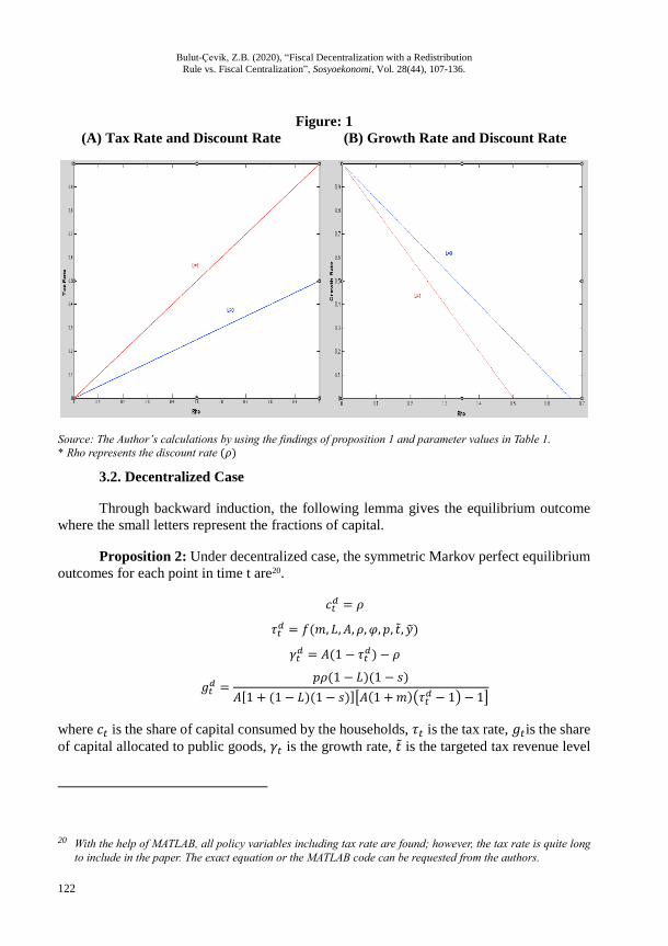
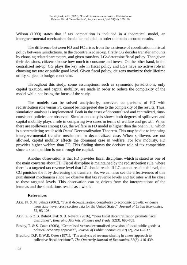
Figure 1 shows the behavior of the relationships between tax rate and discount rate

(Panel A) and growth rate and discount rate (Panel B) for the corner values of selfishness

degree19. The red lines belong to the case of fully selfish government (𝐿 = 1) and blue lines

belong to the case of fully benevolent government (𝐿 = 0). If a fully benevolent government

is switched to a fully selfish government then the slope of the graph increases significantly

in absolute terms. Because fully benevolent government uses its resources more to the public

needs which implies higher growth rate with lower tax rate; whereas fully selfish

government uses resources for itself and so waste the resources which entails smaller growth

rate with higher tax rate.

18 Share of capital that is spent for public good:

𝐺𝑡

𝐾𝑡= 𝑔𝑡

𝑐.

19 𝐿 𝜖 [0,1] so the corner levels are 0 and 1. When 𝐿 = 0, the government is fully benevolent, i.e. it only cares

about the citizens’ utility; however when 𝐿 = 1, the government is fully selfish, i.e. it does not care about the

citizens’ utility but his utility only.



122

Figure: 1

(A) Tax Rate and Discount Rate (B) Growth Rate and Discount Rate

Source: The Author’s calculations by using the findings of proposition 1 and parameter values in Table 1.

* Rho represents the discount rate (𝜌)

3.2. Decentralized Case

Through backward induction, the following lemma gives the equilibrium outcome

where the small letters represent the fractions of capital.

Proposition 2: Under decentralized case, the symmetric Markov perfect equilibrium

outcomes for each point in time t are20.

𝑐𝑡𝑑 = 𝜌

𝜏𝑡𝑑 = 𝑓(𝑚, 𝐿, 𝐴, 𝜌, 𝜑, 𝑝, ��, ��)

𝛾𝑡𝑑 = 𝐴(1 − 𝜏𝑡

𝑑) − 𝜌

𝑔𝑡𝑑 =

𝑝𝜌(1 − 𝐿)(1 − 𝑠)

𝐴[1 + (1 − 𝐿)(1 − 𝑠)][𝐴(1 + 𝑚)(𝜏𝑡𝑑 − 1) − 1]

where 𝑐𝑡 is the share of capital consumed by the households, 𝜏𝑡 is the tax rate, 𝑔𝑡is the share

of capital allocated to public goods, 𝛾𝑡 is the growth rate, �� is the targeted tax revenue level

20 With the help of MATLAB, all policy variables including tax rate are found; however, the tax rate is quite long

to include in the paper. The exact equation or the MATLAB code can be requested from the authors.



123

divided by capital and �� is the targeted income level divided by capital. The superscript ‘d’

represents that the finding belongs to the decentralized case.

Proof: In the Appendix.

As in the centralized case, citizens consume a constant fraction of capital. Despite the

equality in the consumption level since the utility form of the citizens is different, the welfare

level of the citizens for these two cases21 will be different. The constant fraction of capital

shows the time consistency of the variable. Even LG decides to change its policy; the

consumption level of the citizen will not be changed, so LG has no incentive to change its

policy.

All the variables depend on time-independent fraction of capital. However, it is not

easy to interpret the findings so comparative statics analysis is performed and presented as

lemmas below.

Lemma 1: As the selfishness of the politician increases or the degree of spillovers

decreases (i.e. utility taken from the foreign public good is lower), LG increases the tax rate

of its own jurisdiction.

Proof: First order derivative of the tax rate with respect to L and s are positive and

negative respectively.

𝜕𝜏𝑑

𝜕𝐿=

−𝑝𝜌

(𝐿 + 𝑠 − 𝐿𝑠 − 2)[

1

(ℎ1)1/2] > 0 𝑠𝑖𝑛𝑐𝑒 𝐿𝜖[0,1], 𝑠 ∈ [0,0.5]

where ℎ1 is a function of 𝑚, 𝐿, 𝐴, 𝜌, 𝜑, 𝑝, ��, ��

𝜕𝜏𝑑

𝜕𝑠=

𝑝𝜌(𝐿 − 1)2

(𝐿 + 𝑠 − 𝐿𝑠 − 2)[

1

𝐴(ℎ1)12

] < 0 𝑠𝑖𝑛𝑐𝑒 𝐿𝜖[0,1], 𝑠 ∈ [0,0.5]


Higher L means politician wants to spend more tax revenue for his interests while

caring less about the welfare of the citizens, so that the politician sees no harm increasing

the tax rate. For the latter one, firstly LGs have a tendency to increase tax rate because of

higher tax revenue and spending power. However, if tax rate is high enough, that locality

may face two obstacles: losing capital to other locality, which causes reductions in tax

revenue and losing the next election because utility of the citizens will be harmed from high

tax rates. Smaller degree of spillovers (s) indicates low levels of utility taken from the foreign

21 Decentralized and centralized cases.



124

jurisdiction’s public good level, which points out that there is still room for an increase in

tax rate and still locality will not lose capital to other jurisdiction.

Lemma 2: The selfishness of the politician harms the growth rate since as the

selfishness of the politician increases, LGs increase the tax rate. In addition, when the degree

of positive spillovers increases, the growth rate of the economy increases.

Proof: The sign of first-order derivative of growth rate with respect to L is positive

whereas first-order derivative of growth rate with respect to s is negative without any

condition.

𝜕𝛾𝑑

𝜕𝐿=

𝐴𝑝𝜌

(𝐿 + 𝑠 − 𝐿𝑠 − 2)[

1

(ℎ1)1/2] < 0 𝑠𝑖𝑛𝑐𝑒 𝐿𝜖[0,1], 𝑠 ∈ [0,0.5]

𝜕𝛾𝑑

𝜕𝑠=

−𝐴𝑝𝜌(𝐿 − 1)2

(𝐿 + 𝑠 − 𝐿𝑠 − 2)[

1

𝐴(ℎ1)12

] > 0 𝑠𝑖𝑛𝑐𝑒 𝐿𝜖[0,1], 𝑠 ∈ [0,0.5]

Politicians govern localities, and fiscal policies will be affected from their decisions.

Since selfish politicians regard less of citizens, they will increase tax rate and spend tax

revenue for their own interests, which adversely affects the growth rate. This finding

combining with the lemma 1 composes the second result, positive relation between the

degree of spillovers and the growth rate.

Lemma 3: The capital mobility affects the tax rate adversely, in other words as

capital mobility increases, tax rate decreases.

Proof: First order derivative of the tax rate with respect to m is positive.

𝜕𝜏𝑑

𝜕𝑚= −(ℎ2)

12(𝑚 + 1)2 < 0


Capital can move less costly in case of higher capital mobility compared to lower

case. In this study, only tax revenue source for LGs comes with the capital income taxation;

hence in order not to lose more capital, LGs decrease their tax rate when capital mobility

increases.

Lemma 4: As the targeted tax revenue and targeted income level increase, the growth

rate decreases and increases respectively.

Proof: It is the first order derivative of the growth rate with respect to �� and ��.

𝜕𝛾𝑑

𝜕��= −1 < 0 𝑎𝑛𝑑

𝜕𝛾𝑑

𝜕��=

𝜑

𝑝> 0



125

When CG increases the targeted tax revenue, LGs have tendency to increase the tax

rate, which affects the growth adversely. The intuition for the latter one is that if the CG

increases the targeted income level, transfers, distributed to LGs by CG, increase due to the

equity part in redistribution rule. This upturn provides spending more and triggers the growth

rate of the economy.

3.3. Comparison Between FD and FC

This section makes a comparison between the centralized and the decentralized cases

in terms of fiscal policy variables, which are analytically solved. Due to the complexity of

the solutions, some comparisons cannot be concluded in which case simulation analysis is

run by setting some ranges or imposing corner values for the related parameters22. Table 1

presents detailed values for the parameters.

Table: 1

Parameter Values

Parameter Name Value Parameter Name Value

𝜌 Discount Rate 0.01 s Positive Spillovers [0,1] A Level of Technology 0.4 m Capital Mobility [0, ∞]

𝐾0𝑎 Initial Capital 1 �� Targeted Rate [0,0.5]

L Selfishness [0,1] �� Targeted Income 0.3714

In the literature, a discount rate of discrete-time models is assumed to be 0.9923. This

value corresponds to 0.01 in continuous time models. According to the US data, capital-

income ratio is approximately 2.524. By using this capital-income ratio, the level of

technology is calculated as 0.4 since AK-type endogenous growth model is used in this

study. The initial capital level is assumed to be 1 due to the simplicity purposes. Other

possible values for initial capital are tested, however, this does not change the results of

comparisons. In addition to these parameter values, there are some parameters, which are

neither widely used in the literature nor measured in real-time situations such as selfishness

of the politicians, degree of positive spillovers, etc. This problem is overcome by applying

normalized ranges for these parameters. These ranges with intuitions are already explained

in the model part in detail.

Proposition 3: Citizens consume the same and constant fraction of capital in both

decentralized and centralized cases.

𝑐𝑡𝑑 = 𝜌 = 𝑐𝑡

𝑐

22 The MATLAB codes can be provided upon request. 23 Otrok (2001), Jones (2002). 24 This ratio is calculated and preferred in the studies investigating Kaldor’s stylized facts in the literature.



126

This finding can be easily identified from the propositions 1 and 2.

Result 1: When there are spillovers among LGs (𝑠 ≠ 0) and the governments are not

fully selfish (𝐿 ≠ 1), the welfare in FD is higher than the one in FC model despite the tax

rate of FD is also higher than the tax rate of FC.

This result may seem contradictory to the most of the findings in the literature, which

claims in the existence of spillovers, welfare level of FC is higher than the one of FD,

however in Decentralization Theorem or the studies in the literature, there is no

redistribution mechanism that may discipline the local governments. This result shows the

usefulness of FD with redistribution mechanism by not only providing fiscal discipline but

also increasing the welfare. In the redistribution rule of FD case, a target for tax revenue is

set exogenously in efficiency property, however, in FC, the CG is free to choose any tax rate

since they are not tied to any target which leads to higher tax rate in FD than in FC. At first

glance, low levels of tax rate mean an improvement for citizens due to the higher level of

disposable income, but it also implies low levels of tax revenue, and hence low levels of

public good provision. In the model, the objective function of a citizen is not only composed

of consumption level but also public good level at home jurisdiction and neighbor

jurisdiction. Consumption level may increase, because of the increase in disposable income,

but public good provision levels lessen which causes lower levels of utility. In other words,

the increase in consumption level is dominated by the decrease in public good level at home

and neighbor jurisdictions. Hence, in presence of spillovers, public good levels matter more

than consumption levels for citizens.

Result 2: When spillovers are not allowed (s=0) and the governments are not fully

selfish (𝐿 ≠ 1), capital mobility plays a crucial role in welfare comparison between FD with

redistribution rule and FC. In case of low capital mobility, welfare in FD model is higher

than the one in FC, whereas, in case of high capital mobility, welfare in FC model is higher

than the one in FD.

This result is consistent with the finding of Chu and Yang (2012), which shows the

importance of capital mobility when there are no spillovers. In the case of low capital

mobility, tax competition may not be so active which may result with higher tax rate. When

tax competition is high enough, local governments choose low tax rate which results with

under provision of public goods so lower levels of welfare. This result is similar with the

fundamental static result in the tax competition literature25, which tells that tax competition

for mobile capital is harmful since it tends to produce a low tax rate and result in an under

provision of public goods.

25 Wilson (1986), Zodrow and Mieszkowski (1986), Wellisch(2000), Haufler (2001).



127

Result 3: The growth rate of the economy in the case of FD with redistribution rule

is less than the one in case of FC when spillovers are allowed (𝑠 ≠ 0).

This result is an unexpected result since in the literature there are empirical studies

that show both a positive relation between growth rate and FD measures26 and uncorrelated

relation between them27. In this study, the difference comes with the redistribution rule in

which there is a targeted tax rate level that makes the LGs choose around this level. In FC

case, there is no such a target level; this causes to reach a higher growth rate. In other words,

due to fiscal discipline with a redistribution rule, even in case of tax competition, local

governments cannot choose a tax rate whatever level they want, for instance, a low tax rate.

Hence, the growth rate of FC model is higher than the growth rate of FD model.

Result 4: For low levels of selfishness of the politician, as the degree of positive

spillovers increases, tax revenue share for public good provision also increases. On the oher

hand, for high levels of selfishness of the politicians, a higher degree of positive spillovers

lessens the tax revenue share for public good provision.

The intuition behind this result is as follows: Assume the politician has a low

selfishness parameter (low L) then when the degree of positive spillovers increases (i.e. the

utility taken from the foreign public good increases), the LG spends more to public good

provision not to lose the capital of its citizens (i.e. tax revenue share for public good

provision increases). However, there is a threshold level that the LG can do to retain the

capital of its citizens, which depends on selfishness parameter. For higher L, LG does not

try to keep its citizens so decrease its public good spending. Even increasing the degree of

positive spillovers does not change this decrease. This result seems so obvious from the

construction of the model; however, the key point is that the degree of spillovers and degree

of selfishness parameter change simultaneously (i.e. mathematically speaking, it is a second

derivative) and this is not so trivial from the model.

4. Conclusion

In this paper, the effects of FD with a redistribution rule and FC are investigated and

compared. The main contribution of this paper to the literature is introducing a linear

redistribution rule to the FD case in order to investigate whether this mechanism affect the

usual findings in the literature. The necessity of a redistribution rule is widely discussed and

accepted in the literature under the condition that it should have some properties such as

equity, local tax effort, transparency, simplicity, etc. In addition, the theoretical studies of

FD and FC comparisons do not use such a redistribution rule in their models; however,

26 Lin and Liu (2000), Akai and Sakata (2002), Iimi (2005). 27 Davoodi and Zou (1998), Woller and Philips (1998), Thornton (2007).



128

Wilson (1999) states that if tax competition is included in a theoretical model, an

intergovernmental mechanism should be included in order to obtain accurate results.

The difference between FD and FC arises from the existence of coordination in fiscal

policy between jurisdictions. In the decentralized set-up, firstly CG decides transfer amounts

by choosing related parameters, and given transfers, LGs determine fiscal policy. Then given

their decisions, citizens choose how much to consume and invest. On the other hand, in the

centralized set-up, CG plays the key role in fiscal policy and LGs have no active role in

choosing tax rate or public good level. Given fiscal policy, citizens maximize their lifetime

utility subject to budget constraint.

Throughout this study, some assumptions, such as symmetric jurisdictions, only

capital taxation, and capital mobility, are made in order to reduce the complexity of the

model while not losing the focus of the study.

The models can be solved analytically, however, comparisons of FD with

redistribution rule versus FC cannot be interpreted due to the complexity of the results. Thus,

simulation analysis is implemented. Both in the cases of decentralized and centralized, time-

consistent policies are observed. Simulation analysis shows both degrees of spillovers and

capital mobility plays a role in comparing two cases in terms of welfare and growth. When

there are spillovers among LGs, the welfare in FD model is higher than the one in FC, which

is a contradicting result with Oates’ Decentralization Theorem. This may be due to imposing

intergovernmental transfer mechanism in decentralized case. When spillovers are not

allowed, capital mobility affects the dominant case in welfare. For low mobility, FD

provides higher welfare than FC. This finding shows the decisive role of tax competition

since tax competition is run through the capital.

Another observation is that FD provides fiscal discipline, which is stated as one of

the main concerns about FD. Fiscal discipline is maintained by the redistribution rule, where

there is a targeted tax revenue level that LG should reach. If LG cannot reach this level, the

CG punishes the it by decreasing the transfers. So, we can also see the effectiveness of this

punishment mechanism since we observe that tax revenue levels and tax rates will be close

to these targeted levels. This observation can be driven from the interpretations of the

lemmas and the simulations results as a whole.

References

Akai, N. & M. Sakata (2002), “Fiscal decentralization contributes to economic growth: evidence

from state- level cross-section data for the United States”, Journal of Urban Economics,

52, 93-108.

Akin, Z. & Z.B. Bulut-Cevik & B. Neyapti (2016), “Does fiscal decentralization promote fiscal

discipline?”, Emerging Markets, Finance and Trade, 52(3), 690-705.

Besley, T. & S. Coate (2003), “Centralised versus decentralised provision of local public goods: a

political economy approach”, Journal of Public Economics, 87(12), 2611-2637.

Bradford, D.F. & W.E. Oates (1971), “The analysis of revenue sharing in a new approach to

collective fiscal decisions”, The Quarterly Journal of Economics, 85(3), 416-439.



129

Brennan, G. & J.M. Buchanan (1980), The Power to Tax: Analytical Foundations of a Fiscal

Constitution, Cambridge University Press, New York.

Brueckner, J.K. (2003), “Strategic interaction among governments: An overview of empirical

studies”, International Regional Science Review, 26(2), 175-188.

Chu, A.C. & C.C. Yang (2012), “Fiscal centralization versus decentralization: Growth and welfare

effects of spillovers, Leviathan taxation, and capital mobility”, Journal of Urban

Economics, 71, 177-188.

Davoodi, H. & H. Zou (1998), “Fiscal decentralization and economic growth: A Cross- Country

Study”, Journal of Urban Economics, 43, 244-257.

Deveraux, M.P. & B. Lockwood & M. Redeona (2008), “Do countries compete over corporate tax

rates?”, Journal of Public Economics, 92(5), 1210-1235.

Edwards, J. & M. Keen (1996), “Tax competition and Leviathan”, European Economic Review, 40,

113-134.

Epple, D. & T. Nechyba (2004), “Fiscal decentralization”, in: J.V. Henderson & J.F. Thisse (eds.)

Handbook of Regional and Urban Economics, Volume: 4, Chapter: 55.

Eyraud, L. & L. Lusinyan (2011), “Decentralizing Spending More than Revenue: Does It Hurt Fiscal

Performance?”, IMF Working Paper, WP/11/226.

Haufler, A. (2001), Taxation in a global economy, Cambridge Books, Cambridge University Press.

Iimi, A. (2005), “Decentralization and economic growth revisited: an empirical note”, Journal of

Urban Economics, 57, 449-461.

Jones, J.B. (2002), “Has fiscal policy helped stabilized the postwar U.S. economy?”, Journal of

Monetary Policy, 49, 709-746

Klein, P. & J.V. Rios-Rull (2003), “Time-Consistent optimal fiscal policy”, International Economic

Review, 44(4), 1207-1405.

Klein, P. & P. Krusell & J.V. Rios-Rull (2008), “Time-Consistent public policy”, Review of

Economic Studies, 75(3), 789-808.

Krusell, P. & J.V. Rios-Rull (1999), “On the size of US government: Political economy in the

neoclassical growth model”, The American Economic Review, 89(5), 1156-1181.

Lejour, A. & H.A. Verbon (1997), “Tax competition and redistribution in a two-country endogenous-

growth model”, International Tax and Public Finance, 4, 485-497.

Lin, J.Y. & Z. Liu (2000), “Fiscal decentralization and economic growth in China”, Economic

Development and Cultural Change, 49, 1-21.

Lockwood, B. (2006), “Fiscal decentralization: a political economy perspective”, in: E. Ahmad & G.

Brosio (eds.), Handbook of fiscal federalism, Edward Elgar.

Ma, J. (1997), “Intergovernmental Fiscal Transfers in Nine Countries”, prepared for Macroeconomic

Management and Policy Division, Economic Development Institute, The World Bank.

Oates, W.E. (1972), Fiscal federalism, Harcourt-Brace, New York.

Oates, W.E. (1999), “An Essay on Fiscal Federalism”, Journal of Economic Literature, 37(3), 1120-

1149.

Ortigueira, S. & J. Pereira & P. Pichler (2012), “Markov-perfect optimal fiscal policy: The case of

unbalanced budgets”, Universidad Carlos III de Madrid Working Paper, Economic

Series, 12-30.



130

Ortigueira, S. (2006), “Markov-perfect optimal taxation”, Review of Economic Dynamics, 9(1), 153-

178.

Otrok, C. (2001), “On measuring the welfare cost of business cycles”, Journal of Monetary Policy,

47, 61-92.

Persson, T. & G. Tabellini (1992), “The politics of 1992: fiscal policy and European integration”,

Review of Economic Studies, 59, 689-701.

Rauscher, M. (1998), “Leviathan and competition among jurisdictions: the case of benefit taxation”,

Journal of Urban Economics, 44, 59-67.

Rohac, D. (2006), “Evidence and myths about tax competition”, New Perspectives on Political

Economy, 2(2), 86-115.

Shah, A. (1995), “Theory and Practice of Intergovernmental Transfers”, Reforming China’s Public

Finances, 215-234.

Thornton, J. (2007), “Fiscal decentralization and economic growth reconsidered”, Journal of Urban

Economics, 61(1), 64-70.

Tiebout, C.M. (1956), “A Pure Theory of Local Expenditures”, The Journal of Political Economy,

64(5), 416-424.

Wellisch, D. (2000), Theory of Public Finance in a Federal State, Cambridge University Press,

Cambridge.

Wildasin, D.E. (1988), “Nash Equilibria in Models of Fiscal Competition”, Journal of Public

Economics, 35, 229-240.

Wilson, J.D. (1986), “A theory of interregional tax competition”, Journal of Urban Economics, 19,

296-315.

Wilson, J.D. (1999), “Theories of Tax Competition”, National Tax Journal, 52(2), 269-304.

Winner, H. (2005), “Has tax competition emerged in OECD Countries? Evidence form Panel Data”,

International Tax and Public Finance, 12(5), 667-687.

Woller, G.M. & K. Philips (1998), “Fiscal decentralization and LDC growth: an empirical

investigation”, Journal of Development Studies, 34, 138-148.

Xie, D. (1997), “On time inconsistency: A technical issue in Stackelberg differential games”, Journal

of Economic Theory, 76(2), 412-430.

Zodrow, G.R. & P. Mieszkowki (1986), “Pigou, Tiebout, Property Taxation and the Underprovision

of Local Public Goods”, Journal of Urban Economics, 19, 356-370.

Zodrow, G.R. (2003), “Tax Competition and Tax Coordination in the European Union”,

International Tax and Public Finance, 10, 651-671.



131

APPENDIX

Centralized Case:

Citizen’s Problem:

𝑈 = max{𝐶𝑡,𝐾𝑡}

∫ 𝑒−𝜌𝑡[ln 𝐶𝑡 + ln 𝐺𝑡]𝑑𝑡∞

0

subject to

��𝑡 = [𝐴 − 𝑐𝑡 − i𝜏𝑡]𝐾𝑡

Given 𝐺𝑡 , 𝜏𝑡

The current value hamiltonian becomes28

ℋ = ln 𝑐𝑡𝐾𝑡 + ln 𝑔𝑡𝐾𝑡 + 𝜇𝑡(𝐴 − 𝑐𝑡 − i𝜏𝑡)𝐾𝑡

The first order conditions with respect to 𝑐𝑡 , 𝐾𝑡 , 𝜇𝑡 are as follows:

𝜕ℋ𝑡

𝜕𝑐𝑡=

1

𝑐𝑡𝐾𝑡𝐾𝑡 − 𝜇𝑡𝐾𝑡

𝜕ℋ𝑡

𝜕𝐾𝑡=

1

𝑐𝑡𝐾𝑡𝑐𝑡 + 𝜇𝑡(𝐴 − 𝑐𝑡 − 𝜏𝑡) = 𝜇𝑡𝜌 − ��𝑡

𝜕ℋ𝑡

𝜕𝜇𝑡= 𝐾𝑡(𝐴 − 𝑐𝑡 − 𝜏𝑡) = ��𝑡

The first order conditions, transversality condition (lim𝑡→∞

𝑒−𝜌𝑡𝜇𝑡𝐾𝑡 = 0) and the firm

problem’s result, (𝑖 = 𝐴), give the following result

𝐾𝑡𝜇𝑡𝜌 − 1 = 𝜇𝑡��𝑡 + 𝐾𝑡��𝑡

Integrating this result with respect to time shows that consumption is a constant

fraction of capital level

𝐶𝑡 = 𝜌𝐾𝑡

28 Denote 𝑔𝑡 =

𝐺𝑡𝐾𝑡

⁄ as the share of capital allocated to public goods and 𝑐𝑡 =𝐶𝑡

𝐾𝑡⁄ as the share of capital

consumed by the households. (Chu & Yang, 2012).



132

Since 𝜇0 = (𝜌𝐾0)−1 is predetermined since 𝜇0 cannot be controlled by the

government. 𝐾0 is given, 𝜌 is a parameter and so ct is independent from the government

policy which means it is time consistent.

The growth rate

𝛾𝑡 = 𝐴 − 𝜌 − 𝐴𝜏𝑡

Central Government’s Problem:

𝑉 = max𝐺𝑡,𝜏𝑡,𝑅𝑡,𝐾𝑡

(1 − 𝐿)𝑈 + 𝐿 ∫ 𝑒−𝜌𝑡∞

0

[ln 𝑅𝑡]𝑑𝑡

subject to

𝐺𝑡 + 𝑅𝑡 = 𝑁𝑡 = 𝐴𝜏𝑡𝐾𝑡 = 𝐴(𝑔𝑡 + 𝑟𝑡)𝐾𝑡

��𝑡 = [𝐴 − 𝜌 − 𝑖𝜏𝑡]𝐾𝑡

where 𝑈 = ln 𝐶𝑡 + ln 𝐺𝑡

The current value Hamiltonian becomes

ℋ = (1 − 𝐿)[ln ctKt + ln gtKt] + L[ln rtKt] + μtKt (A − ρ − iτt) + λtKt(τt − gt − rt)

First order conditions with respect to 𝜏𝑡 , 𝐾𝑡 , 𝑔𝑡 , 𝑟𝑡 , ��𝑡 , 𝜆𝑡 are as follows respectively:

𝜕ℋ𝑡

𝜕𝜏𝑡= −��𝑡𝐾𝑡 + λtKt

𝜕ℋ𝑡

𝜕𝐾𝑡=

1 − 𝐿

ctKtct +

1 − 𝐿

gtKtgt +

𝐿

rtKtrt + μt(A − ρ − τt)+λt(τt − gt − rt) = μtρ − μt

𝜕ℋ𝑡

𝜕𝑔𝑡=

1 − 𝐿

gtKtKt − λtKt = 0

𝜕ℋ𝑡

𝜕𝑟𝑡=

𝐿

rtKtKt − λtKt = 0

𝜕ℋ𝑡

𝜕��𝑡= Kt(A − ρ − τt) = Kt

𝜕ℋ𝑡

𝜕𝜆𝑡= Kt(τt − gt − rt) = 0


𝑒−𝜌𝑡��𝑡𝐾𝑡 = 0) and the firm

problem’s result, (𝑟 = 𝐴), give the following result

μtKt − μtKt = μtKtρ − (2 − L)



133

Integrating with respect to time, then μtKt =(2 − 𝐿)

𝜌⁄ . Substituting this into the

first order conditions, choice variables will be as follows:

𝜏𝑡 =𝜌

𝐴(𝐴 + 1 − 𝐿)

𝑔𝑡 =𝜌(1 − 𝐿)

(𝐴 + 1 − 𝐿)

𝛾𝑡 = 𝐴 − 𝜌 −𝜌

𝐴 + 1 − 𝐿

Decentralized Case:

Citizen’s Problem:

𝑈 = max{𝐶𝑡,𝐾𝑡,𝜃𝑡}

∫ 𝑒−𝜌𝑡[ln 𝐶𝑡 + (1 − s)ln 𝐺𝑡 + 𝑠ln𝐺𝑡∗]𝑑𝑡

∞

0

subject to

𝐾�� = (1 − 𝜏𝑡)𝑖𝐷𝑡 + (1 − 𝜏𝑡∗) 𝑖∗𝐹𝑡 – 𝐶𝑡 − 𝐾𝑡

(𝜃𝑡)2

𝑚⁄

Given 𝐺𝑡 , 𝐺𝑡∗, 𝜏𝑡, 𝜏𝑡

∗

The current value hamiltonian becomes

ℋ =ln 𝑐𝑡𝐾𝑡 + (1 − s) ln 𝑔𝑡𝐾𝑡 + 𝑠 ln 𝑔𝑡

∗𝐾𝑡∗ +

𝜇𝑡 (𝐴 − 𝑐𝑡 − (1 − 𝜃𝑡)𝑖𝜏𝑡 − 𝜃𝑡𝑖∗𝜏𝑡∗ −

(𝜃𝑡)2

𝑚⁄ ) 𝐾𝑡

The first order conditions with respect to 𝑐𝑡 , 𝐾𝑡 , 𝜃𝑡 , 𝜇𝑡 are as follows:

𝜕ℋ𝑡

𝜕𝑐𝑡=

1

𝑐𝑡𝐾𝑡𝐾𝑡 − 𝜇𝑡𝐾𝑡 = 0

𝜕ℋ𝑡

𝜕𝐾𝑡=

1

𝑐𝑡𝐾𝑡𝑐𝑡 +

1

𝑔𝑡𝐾𝑡𝑔𝑡 + 𝜇𝑡 (𝐴 − 𝑐𝑡 − (1 − 𝜃𝑡)𝑖𝜏𝑡 − 𝜃𝑡𝑖∗𝜏𝑡

∗ −(𝜃𝑡)2

𝑚⁄ ) = 𝜇𝑡𝜌 − ��𝑡

𝜕ℋ𝑡

𝜕𝜃𝑡= 𝜇𝑡 (𝑖𝜏𝑡 − 𝑖∗𝜏𝑡

∗ − 2𝜃𝑡

𝑚⁄ ) = 0

𝜕ℋ𝑡

𝜕𝜇𝑡= 𝐾𝑡 (𝐴 − 𝑐𝑡 − (1 − 𝜃𝑡)𝑖𝜏𝑡 − 𝜃𝑡𝑖∗𝜏𝑡

∗ −(𝜃𝑡)2

𝑚⁄ ) = ��𝑡


𝑒−𝜌𝑡𝜇𝑡𝐾𝑡 = 0) and the firm

problem’s finding, (𝑖 = 𝐴 = 𝑖∗), give the following results



134

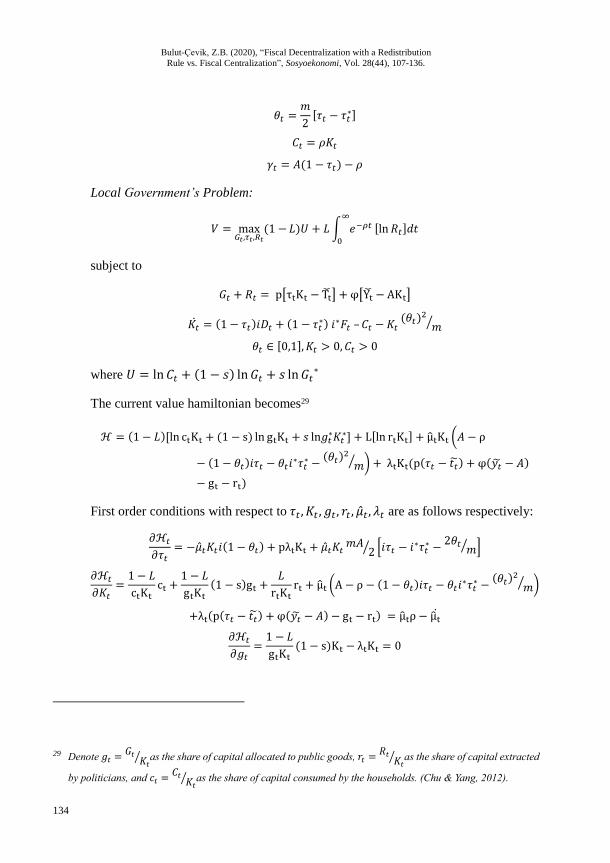
𝜃𝑡 =𝑚

2[𝜏𝑡 − 𝜏𝑡

∗]

𝐶𝑡 = 𝜌𝐾𝑡

𝛾𝑡 = 𝐴(1 − 𝜏𝑡) − 𝜌

Local Government’s Problem:

𝑉 = max𝐺𝑡,𝜏𝑡,𝑅𝑡

(1 − 𝐿)𝑈 + 𝐿 ∫ 𝑒−𝜌𝑡∞

0

[ln 𝑅𝑡]𝑑𝑡

subject to

𝐺𝑡 + 𝑅𝑡 = p[τtKt − Tt] + φ[Yt − AKt]

𝐾�� = (1 − 𝜏𝑡)𝑖𝐷𝑡 + (1 − 𝜏𝑡∗) 𝑖∗𝐹𝑡 – 𝐶𝑡 − 𝐾𝑡

(𝜃𝑡)2

𝑚⁄

𝜃𝑡 ∈ [0,1], 𝐾𝑡 > 0, 𝐶𝑡 > 0

where 𝑈 = ln 𝐶𝑡 + (1 − 𝑠) ln 𝐺𝑡 + 𝑠 ln 𝐺𝑡∗

The current value hamiltonian becomes29

ℋ = (1 − 𝐿)[ln ctKt + (1 − s) ln gtKt + 𝑠 ln𝑔𝑡∗𝐾𝑡

∗] + L[ln rtKt] + μtKt (𝐴 − ρ

− (1 − 𝜃𝑡)𝑖𝜏𝑡 − 𝜃𝑡𝑖∗𝜏𝑡∗ −

(𝜃𝑡)2

𝑚⁄ ) + λtKt(p(𝜏𝑡 − 𝑡��) + φ(𝑦�� − 𝐴)

− gt − rt)

First order conditions with respect to 𝜏𝑡 , 𝐾𝑡 , 𝑔𝑡 , 𝑟𝑡 , ��𝑡 , 𝜆𝑡 are as follows respectively:

𝜕ℋ𝑡

𝜕𝜏𝑡= −��𝑡𝐾𝑡𝑖(1 − 𝜃𝑡) + pλtKt + ��𝑡𝐾𝑡

𝑚𝐴2⁄ [𝑖𝜏𝑡 − 𝑖∗𝜏𝑡

∗ −2𝜃𝑡

𝑚⁄ ]

𝜕ℋ𝑡

𝜕𝐾𝑡=

1 − 𝐿

ctKtct +

1 − 𝐿

gtKt

(1 − s)gt +𝐿

rtKtrt + μt (A − ρ − (1 − 𝜃𝑡)𝑖𝜏𝑡 − 𝜃𝑡𝑖∗𝜏𝑡

∗ −(𝜃𝑡)2

𝑚⁄ )

+λt(p(𝜏𝑡 − 𝑡��) + φ(𝑦�� − 𝐴) − gt − rt) = μtρ − μt

𝜕ℋ𝑡

𝜕𝑔𝑡=

1 − 𝐿

gtKt(1 − s)Kt − λtKt = 0

29 Denote 𝑔𝑡 =

𝐺𝑡𝐾𝑡

⁄ as the share of capital allocated to public goods, 𝑟𝑡 =𝑅𝑡

𝐾𝑡⁄ as the share of capital extracted

by politicians, and 𝑐𝑡 =𝐶𝑡

𝐾𝑡⁄ as the share of capital consumed by the households. (Chu & Yang, 2012).



135

𝜕ℋ𝑡

𝜕𝑟𝑡=

𝐿

rtKtKt − λtKt = 0

𝜕ℋ𝑡

𝜕��𝑡= Kt (𝐴 − ρ − (1 − 𝜃𝑡)𝑖𝜏𝑡 − 𝜃𝑡𝑖∗𝜏𝑡

∗ −(𝜃𝑡)2

𝑚⁄ ) = Kt

𝜕ℋ𝑡

𝜕𝜆𝑡= Kt(p(𝜏𝑡 − 𝑡��) + φ(𝑦�� − 𝐴) − gt − rt) = 0

The first order conditions with respect to 𝜏𝑡 , 𝐾𝑡 , 𝑔𝑡 , 𝑟𝑡 , ��𝑡 , 𝜆𝑡 transversality condition

(lim𝑡→∞

𝑒−𝜌𝑡��𝑡𝐾𝑡 = 0) and the firm problem’s result, (𝑟 = 𝐴), give the following result

μtKt − μtKt = μtKtρ − (2 − L)

Integrating with respect to time, then μtKt =(2 − 𝐿)

𝜌⁄ . Substituting this into the

first order conditions, choice variables will be as follows:

𝐺𝑡 =𝑝𝜌(1 − 𝐿)(1 − 𝑠)

𝐴[1 + (1 − 𝐿)(1 − 𝑠)][𝐴(1 + 𝑚)(𝜏𝑡 − 1) − 1]𝐾𝑡

𝑅𝑡 =𝑝𝜌𝐿

𝐴[1 + (1 − 𝐿)(1 − 𝑠)][𝐴(1 + 𝑚)(𝜏𝑡 − 1) − 1]𝐾𝑡

By substituting these equations into the first constraint of local government’s

problem:

𝐺𝑡 + 𝑅𝑡 =𝑝𝜌(1 − 𝑠 + 𝑠𝐿)

𝐴[1 + (1 − 𝐿)(1 − 𝑠)][𝐴(1 + 𝑚)(𝜏𝑡 − 1) − 1]𝐾𝑡

= (p(𝜏𝑡 − 𝑡��) + φ(𝑦�� − 𝐴))𝐾𝑡

By simplifying the above equation, we can find the optimal tax rate by the help of

MATLAB. MATLAB gives long and complicated two roots for optimal tax rate. Under

specific parameters, the first root gives plausible values as a tax rate30.

Central Government’s Problem:

max𝑝,𝜑

𝑈 + 𝑈∗

subject to

A𝜏𝑡𝐾𝑡 + A𝜏𝑡∗𝐾𝑡

∗ = p[τtKt − Tt] + φ[Yt − AKt] + p[τt∗Kt

∗ − Tt∗] + φ[Yt

∗− AKt

∗]

30 Second root is the opposite of the first root in sign.



136

𝑝 ∈ [0,1], 𝜑 ∈ [0,1]

where 𝑈 and 𝑈∗are objective functions of two citizens.

Imposing symmetric jurisdictions assumption (τt = τt∗, Kt = Kt

∗) and the

multiplication logarithm rule31 then taking the first-order condition with respect to 𝑝 and 𝜑

gives the following equation:

𝜕𝜏

𝜕𝑝[

𝜕𝜏

𝜕𝜑(𝑝 − 𝐴) + �� − 𝐴] =

𝜕𝜏

𝜕𝜑[𝜕𝜏

𝜕𝑝(𝑝 − 𝐴) + 𝜏 − ��]

By solving this equation, we can find optimal 𝑝 in terms of 𝜑. By substituting optimal

𝑝 to the budget constraint, we are able to find optimal 𝜑 with the help of MATLAB.

31 𝑙𝑜𝑔(𝐴 ∗ 𝐵) = 𝑙𝑜𝑔(𝐴) + 𝑙𝑜𝑔 (𝐵).

Documents

Fiscal Decentralization with a Redistribution Rule vs