Embed Size (px)
Citation preview
BRNO UNIVERSITY OF TECHNOLOGY
FACULTY OF CIVIL ENGINEERING
FATIGUE PROPERTIES OF STEEL S355
BACHELOR THESIS
AUTHOR D. Álvaro Martín González
SUPERVISOR SUPERVISOR SPECIALIST:
Assoc. Prof. Stanislav Seitl, Ph. D. Ing. Petr Miarka
BRNO, CZECH REPUBLIC 2018
ÁLVARO MARTÍN GONZÁLEZ 2
ABSTRACT
This thesis is focused in the numerical simulation by software ANSYS (finite
elements method) of fatigue properties such as the Wöhler’s curves and crack
propagation rates and Fracture Mechanics properties such as stress intensity factors and
𝑇-stresses in Compact Tension specimen.
Two grades of structural steel S355 will be evaluated in order to study the
influence of the material in the fatigue properties.
Calibration curves will be used for evaluation of data, comparing the results with
data published in literature.
KEYWORDS
Fatigue, Finite Element Method, Fracture Mechanics, Stress Intensity Factor, 𝑇-
stress, Crack Propagation Rate, Wöhler’s Curves, Compact Tension Specimen, Structural
Steel S355, ASTM, EN.
RESUMEN
Éste proyecto se basa en la simulación numérica con ANSYS (software para el
análisis mediante el método de los elementos finitos) de propiedades de la fatiga tales
como las curvas de Wöhler y velocidades de propagación de grieta, y propiedades de la
Mecánica de la Fractura tales como factores intensidad de tensiones y tensiones-𝑇
mediante probetas CT (del inglés, Compact Tension).
Se evaluarán dos grados diferentes de acero estructural S355 con la finalidad de
estudiar la influencia del material en dichas propiedades.
Para la evaluación de los resultados numéricos se utilizarán curvas de calibración,
comparando, los mismos, con datos publicados en diferentes artículos.
PALABRAS CLAVE
Fatiga, Método de los Elementos Finitos, Mecánica de la Fractura, Factor
Intensidad de Tensiones, Tensión T, Velocidad de Propagación de Grieta, Curvas de
Wöhler, Probeta CT, Acero Estructural S355, ASTM, EN.
ÁLVARO MARTÍN GONZÁLEZ 3
BIBLIOGRAPHIC CITATION
Álvaro Martín González, Fatigue properties of steel S355 measured by Compact Tension
test. Brno, 2018. 63 p., 9 p. of attachments. Bachelor Thesis. Brno University of
Technology, Faculty of civil engineering, Supervisor: Assoc. Prof. Stanislav Seitl, Ph. D.
Supervisor Specialist: Ing. Petr Miarka.
ÁLVARO MARTÍN GONZÁLEZ 4
The present thesis is the final part of my studies in Mechanical Engineering (2014-
2018) at the University of Oviedo. It has been held in Brno, Czech Republic, during
Erasmus+ mobility in collaboration with staff from Faculty of civil engineering, Brno
University of Technology.
I would like to thank the invaluable help of my tutors, who have made it possible
for me to carry out this project; Stanislav Seitl, Petr Miarka and María Jesús Lamela Rey.
Also, to my parents and my sister. It would not have been possible to carry out this project
without their help and support.
ACKNOWLEDGEMENT
The author acknowledges the support of Czech Sciences Foundation project
under the contract No. 17-01589S. This thesis has been carried out under the project
No. LO1408 "AdMaS UP − Advanced Materials, Structures and Technologies", supported
by Ministry of Education, Youth and Sports under the „National Sustainability Programme
I".
ÁLVARO MARTÍN GONZÁLEZ 5
INDEX
1. INTRODUCTION ................................................................................................................................... 7
2. THEORETICAL BACKGROUND ........................................................................................................ 8
2.1 Linear Elastic Fracture Mechanics ......................................................................................... 8
2.1.1 The stress analysis of cracks................................................................................................ 8
2.1.2 The stress intensity factor .................................................................................................... 9
2.1.3 T-stress ..................................................................................................................................... 10
2.1.4 Crack-tip plasticity ............................................................................................................... 10
2.2 Elastic-Plastic Fracture Mechanics...................................................................................... 11
2.2.1 Crack-Tip Opening Displacement ................................................................................... 11
2.3 Fatigue .......................................................................................................................................... 12
2.3.1 Fatigue regimes ..................................................................................................................... 12
2.3.2 Fatigue failure models ........................................................................................................ 12
2.3.3 The Compact Test specimen (ASTM E647) ................................................................... 24
2.3.4 Structural steel S355 (EN 10025) .................................................................................... 26
3. AIM OF THESIS ................................................................................................................................... 30
4. NUMERICAL MODELING IN ANSYS ............................................................................................ 31
4.1 Prior set up .................................................................................................................................. 31
4.2 Pre-processor ............................................................................................................................. 31
4.2.1 Specimen ................................................................................................................................. 31
4.2.2 Element type ........................................................................................................................... 31
4.2.3 Material .................................................................................................................................... 32
4.2.4 Modelling of the specimen ................................................................................................ 33
4.2.5 Meshing .................................................................................................................................... 37
4.2.6 Boundary conditions ............................................................................................................ 37
4.3 Solve .............................................................................................................................................. 38
4.4 Post-processor ........................................................................................................................... 40
4.4.1 Stress Intensity Factor ......................................................................................................... 40
4.4.2 T-stress ..................................................................................................................................... 41
5. NUMERICAL RESULTS ...................................................................................................................... 43
5.1 Stress Intensity Factors ........................................................................................................... 43

ÁLVARO MARTÍN GONZÁLEZ 6
5.1.1 ASTM literature calculations ............................................................................................. 43
5.1.2 Knésl and Bednar literature calculations ...................................................................... 44
5.1.3 ANSYS calculations .............................................................................................................. 44
5.2 T-stresses ..................................................................................................................................... 45
5.2.1 Knésl and Bednar literature calculations ...................................................................... 45
5.2.2 ANSYS calculations .............................................................................................................. 46
6. VALUES OF S355 PUBLISHED IN LITERATURE ........................................................................ 48
6.1 Experimental data of S-N curves published in literature ........................................... 48
6.2 Experimental data of crack propagation rates published in literature ................. 49
7. EVALUATION OF S355 MEASURED DATA AT INSTITUTE OF PHYSICS OF
MATERIALS .................................................................................................................................................... 50
7.1 Experimental data of S-N curves from IPM ..................................................................... 50
7.2 Experimental data of crack propagation rates from IPM .......................................... 52
8. COMPARISON AND DISCUSSION OF THE RESULTS ............................................................ 55
8.1 Comparison of curves from ANSYS and literature ....................................................... 55
8.1.1 Comparison of Stress Intensity Factor ........................................................................... 55
8.1.2 Comparison of T-stress ....................................................................................................... 56
8.2 Comparison of Stress-Number of cycles curves ........................................................... 56
8.3 Comparison of crack propagation rate curves .............................................................. 58
9. CONCLUSIONS ................................................................................................................................... 59
10. APPENDIX ........................................................................................................................................ 60
10.1 APPENDIX I - Nomenclature ................................................................................................ 60
10.2 APPENDIX II - List of figures ................................................................................................. 61
10.3 APPENDIX III - List of tables ................................................................................................. 62
10.4 APPENDIX IV - List of graphs ............................................................................................... 63
10.5 APPENDIX V - Macro for the CT specimen ..................................................................... 65
10.5.1 Prior setup ............................................................................................................................... 65
10.5.2 Preprocessor ........................................................................................................................... 65
10.5.3 Solve .......................................................................................................................................... 67
10.5.4 Postprocessing ....................................................................................................................... 67
11. REFERENCES .................................................................................................................................... 69
12. CURRICULUM VITAE .................................................................................................................... 71
ÁLVARO MARTÍN GONZÁLEZ 7
1. INTRODUCTION
In general, perhaps fatigue is the most important failure mode to be considered
in mechanical and structural design. For some products, fatigue accounts for more than
80 % of all observed service failures.
Moreover, fatigue and fracture failures are sometimes catastrophic, occurring
without warning and causing significant property damage and loss of life. Design for
fatigue avoidance is difficult because the fatigue stresses are complicated random
processes, the fatigue process is influenced by many factors, and many of the factors are
subjected to considerable uncertainty. [1]
Structural steel and, in particular, mild steel such as S355, is used for bolts, chains,
connecting rods, and, in civil engineering, for railroad axes, and metallic structures (such
as towers and bridges), i.e. allows designing lighter, slenderer and simpler structures with
high structural performance.
When those large structures are designed and built, different individual
components are used and joined together (usually by welding). In these situations, it
does not matter what care you have and how stricter is the quality control applied, the
existence of small defects (cracks) is unavoidable. The dimensions of the pre-existing
cracks are usually defined by the detection limit of the non-destructive testing method
applied in quality control after manufacturing or in regular inspections in service. [2]
Since the first research on metal fatigue began in the 18th century (Wilhelm Albert
[3]), a very large number of researchers from all over the world have contributed to the
knowledge base that has been amassedis.
By far, the most influential person at the beginning of the systematic study of
fatigue was August Wöhler.
The study of fracture mechanics, which describe the physics and mathematics
behind the growth of cracks in brittle solids, was begun by Alan Griffith in 1921 [4] but is
in the early 1960s when Paris and others [5] demonstrated that fracture mechanics is a
useful tool for characterizing crack growth by fatigue. Since that time, the application of
fracture mechanics to fatigue problems has become routine.
On the other hand, the major advance in the statistical treatment of fatigue data
occurred with the work of Waloddi Weibull in the late 1930’s [6]. Also, the ASTM has
played an active role in development of statistical methods of fatigue data analysis dating
back to 1951 [7], [8].
Because of this, fatigue problems have been traditionally faced from two different
points of view: the Wöhler’s curves-based (statistical) and the fracture mechanics-based
approaches, that constitute two complementary but comprehensive methods to face
fatigue lifetime prediction of mechanical and structural elements.
ÁLVARO MARTÍN GONZÁLEZ 8
2. THEORETICAL BACKGROUND
2.1 Linear Elastic Fracture Mechanics
Linear elastic fracture mechanics (LEFM) is valid only as long as nonlinear material
deformation is confined to a small region surrounding the crack tip.
There are two approaches to linear elastic fracture mechanics: the energy (𝐺) and
stress intensity. In the case of the perfectly elastic materials, both factors are related in
Equation (1). This thesis is not focused in the energy approach.
𝐺 =𝐾2
𝐸´ , (1)
where:
𝐸′ = 𝐸 Young‘s modulus for plane stress and
𝐸′ = 𝐸
1−𝜗 Young’s modulus for plane strain, where 𝜗 is Poisson’s ratio.
Griffith observed in 1920 that the discrepancy between the actual strengths of
brittle materials and theoretical estimates was due to flaws in these materials. Fracture
cannot occur unless the stress at the atomic level exceeds the cohesive strength of the
material. Thus, the flaws must lower the global strength by magnifying the stress locally.
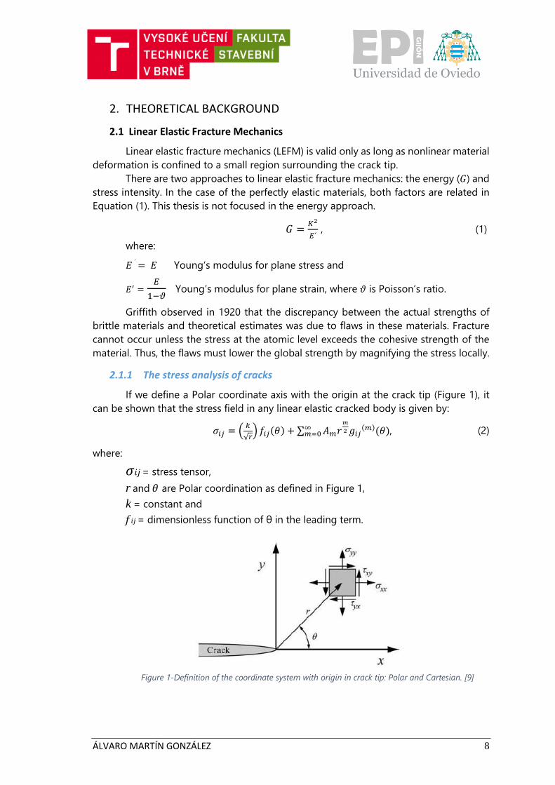
2.1.1 The stress analysis of cracks
If we define a Polar coordinate axis with the origin at the crack tip (Figure 1), it
can be shown that the stress field in any linear elastic cracked body is given by:
𝜎𝑖𝑗 = (𝑘
√𝑟) 𝑓𝑖𝑗(𝜃) + ∑ 𝐴𝑚𝑟
𝑚
2 𝑔𝑖𝑗(𝑚)(𝜃)∞
𝑚=0 , (2)
where:
𝜎𝑖𝑗 = stress tensor,
r and 𝜃 are Polar coordination as defined in Figure 1,
k = constant and
𝑓𝑖𝑗 = dimensionless function of θ in the leading term.
Figure 1-Definition of the coordinate system with origin in crack tip: Polar and Cartesian. [9]
ÁLVARO MARTÍN GONZÁLEZ 9
Therefore, a stress singularity exists at the tip of an elastic crack because the stress
field in any linear elastic cracked body solution contains a leading term that is
proportional to 1
√𝑟 . As 𝑟 → 0, the leading term approaches infinity so stress is asymptotic
to r = 0 (regardless of the configuration of the cracked body) as shown in Equation (2).
2.1.2 The stress intensity factor
There are three types of loading that a crack can experience, as Figure 2 illustrates.
Mode I loading, where the principal load is applied normal to the crack plane, tends to
open the crack. Mode II corresponds to in-plane shear loading and tends to slide one
crack face with respect to the other. Mode III refers to out-of-plane shear. A cracked body
can be loaded in any one of these modes, or a combination of two or three modes.
Figure 2-The three modes of loading that a crack can experience. [9]
Each mode of loading produces the singularity at the crack tip, but the
proportionality constants 𝑘 and 𝑓𝑖𝑗 depend on the mode. It is convenient at this point to
replace 𝑘 by the stress intensity factor (SIF) 𝐾, where 𝐾 = 𝑘√2𝜋 . The stress intensity factor
is usually given a subscript to denote the mode of loading, i.e., 𝐾𝐼, 𝐾𝐼𝐼 , or 𝐾𝐼𝐼𝐼 .
The stress intensity factor defines the amplitude of the crack-tip singularity. That
is, stresses near the crack tip increase in proportion to 𝐾. Moreover, the stress intensity
factor completely defines the crack tip conditions; if 𝐾 is known, it is possible to solve for
all components of stress, strain, and displacement as a function of 𝑟 and 𝜃. This single-
parameter description of crack tip conditions turns out to be one of the most important
concepts in fracture mechanics.
In this thesis, only pure Mode I is considered, since in the evaluation with Compact
Tension Specimen, the load is applied normal to the crack plane. Because of this, in the
following, when referring to “SIF”, it is understood 𝐾𝐼.
ÁLVARO MARTÍN GONZÁLEZ 10
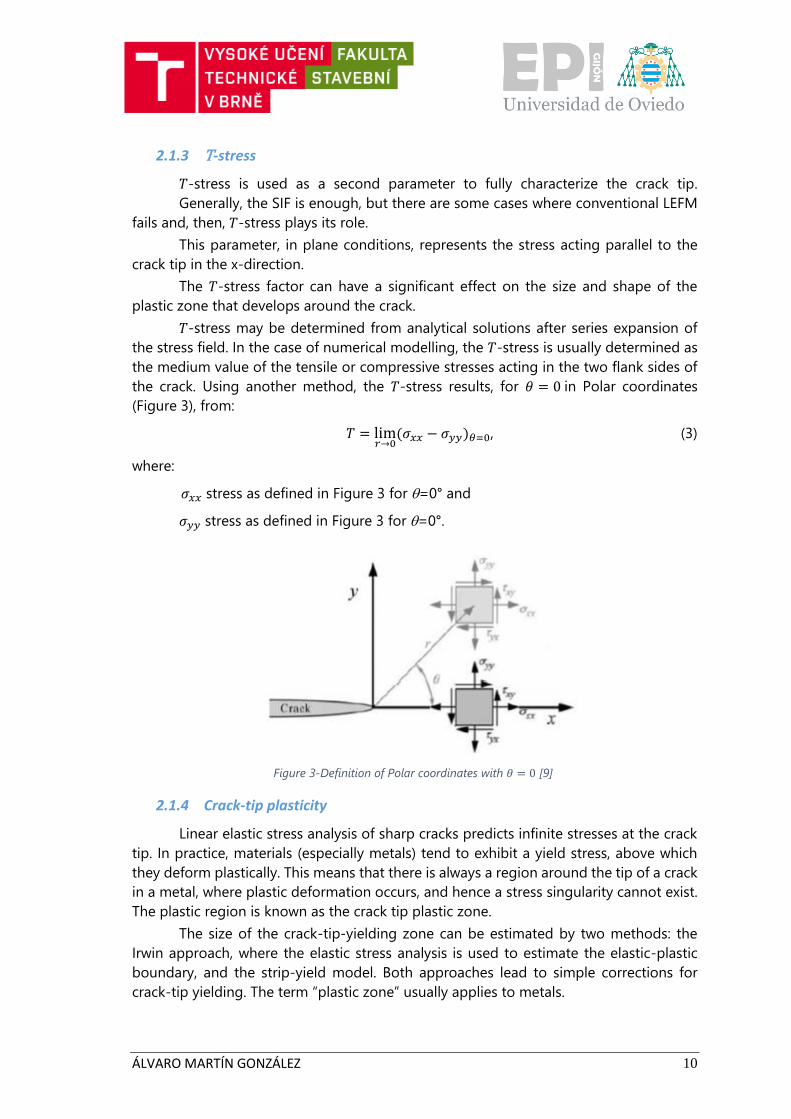
2.1.3 T-stress
𝑇-stress is used as a second parameter to fully characterize the crack tip.
Generally, the SIF is enough, but there are some cases where conventional LEFM
fails and, then, 𝑇-stress plays its role.
This parameter, in plane conditions, represents the stress acting parallel to the
crack tip in the x-direction.
The 𝑇-stress factor can have a significant effect on the size and shape of the
plastic zone that develops around the crack.
𝑇-stress may be determined from analytical solutions after series expansion of
the stress field. In the case of numerical modelling, the 𝑇-stress is usually determined as
the medium value of the tensile or compressive stresses acting in the two flank sides of
the crack. Using another method, the 𝑇-stress results, for 𝜃 = 0 in Polar coordinates
(Figure 3), from:
𝑇 = lim𝑟→0
(𝜎𝑥𝑥 − 𝜎𝑦𝑦)𝜃=0, (3)
where:
𝜎𝑥𝑥 stress as defined in Figure 3 for =0° and
𝜎𝑦𝑦 stress as defined in Figure 3 for =0°.
Figure 3-Definition of Polar coordinates with 𝜃 = 0 [9]
2.1.4 Crack-tip plasticity
Linear elastic stress analysis of sharp cracks predicts infinite stresses at the crack
tip. In practice, materials (especially metals) tend to exhibit a yield stress, above which
they deform plastically. This means that there is always a region around the tip of a crack
in a metal, where plastic deformation occurs, and hence a stress singularity cannot exist.
The plastic region is known as the crack tip plastic zone.
The size of the crack-tip-yielding zone can be estimated by two methods: the
Irwin approach, where the elastic stress analysis is used to estimate the elastic-plastic
boundary, and the strip-yield model. Both approaches lead to simple corrections for
crack-tip yielding. The term “plastic zone” usually applies to metals.
ÁLVARO MARTÍN GONZÁLEZ 11
2.2 Elastic-Plastic Fracture Mechanics
Elastic-plastic fracture mechanics (EPFM) applies to materials that exhibit time-
independent, nonlinear behavior (i.e., plastic deformation).
As in LEFM, there exists two approaches: the crack-tip-opening displacement
(CTOD) and the 𝐽 contour integral (energetic criterion).
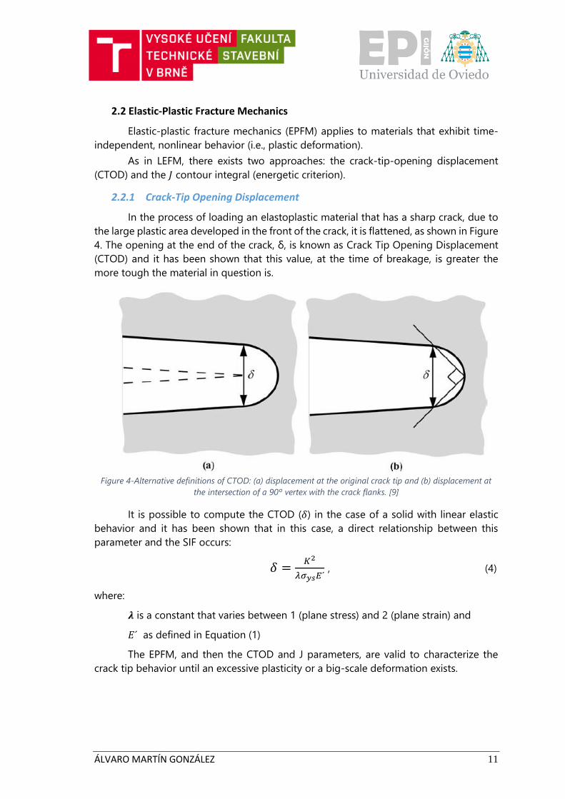
2.2.1 Crack-Tip Opening Displacement
In the process of loading an elastoplastic material that has a sharp crack, due to
the large plastic area developed in the front of the crack, it is flattened, as shown in Figure
4. The opening at the end of the crack, δ, is known as Crack Tip Opening Displacement
(CTOD) and it has been shown that this value, at the time of breakage, is greater the
more tough the material in question is.
Figure 4-Alternative definitions of CTOD: (a) displacement at the original crack tip and (b) displacement at
the intersection of a 90º vertex with the crack flanks. [9]
It is possible to compute the CTOD (𝛿) in the case of a solid with linear elastic
behavior and it has been shown that in this case, a direct relationship between this
parameter and the SIF occurs:
𝛿 =𝐾2
𝜆𝜎𝑦𝑠𝐸´ , (4)
where:
𝝀 is a constant that varies between 1 (plane stress) and 2 (plane strain) and
𝐸´ as defined in Equation (1)
The EPFM, and then the CTOD and J parameters, are valid to characterize the
crack tip behavior until an excessive plasticity or a big-scale deformation exists.
ÁLVARO MARTÍN GONZÁLEZ 12
2.3 Fatigue
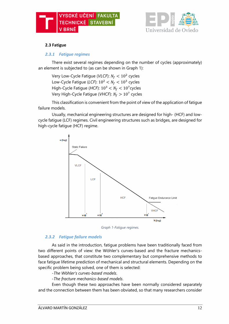
2.3.1 Fatigue regimes
There exist several regimes depending on the number of cycles (approximately)
an element is subjected to (as can be shown in Graph 1):
Very Low-Cycle Fatigue (VLCF): 𝑁𝑓 < 102 cycles
Low-Cycle Fatigue (LCF): 102 < 𝑁𝑓 < 103 cycles
High-Cycle Fatigue (HCF): 103 < 𝑁𝑓 < 107cycles
Very High-Cycle Fatigue (VHCF): 𝑁𝑓 > 107 cycles
This classification is convenient from the point of view of the application of fatigue
failure models.
Usually, mechanical engineering structures are designed for high- (HCF) and low-
cycle fatigue (LCF) regimes. Civil engineering structures such as bridges, are designed for
high-cycle fatigue (HCF) regime.
Graph 1-Fatigue regimes.
2.3.2 Fatigue failure models
As said in the introduction, fatigue problems have been traditionally faced from
two different points of view: the Wöhler’s curves-based and the fracture mechanics-
based approaches, that constitute two complementary but comprehensive methods to
face fatigue lifetime prediction of mechanical and structural elements. Depending on the
specific problem being solved, one of them is selected:
-The Wöhler’s curves-based models.
-The fracture mechanics-based models.
Even though these two approaches have been normally considered separately
and the connection between them has been obviated, so that many researchers consider
ÁLVARO MARTÍN GONZÁLEZ 13
them as two completely different problems, in Castillo et al. [10] a clear connection
between the two models is presented, showing that they share common information,
which is useful in applications.
2.3.2.1 Fracture mechanics approach
The crack-growth curves are of interest for this approach. This approach is
suitable for LCF regimes.
➢ The functional-relationships of the crack growth per cycle
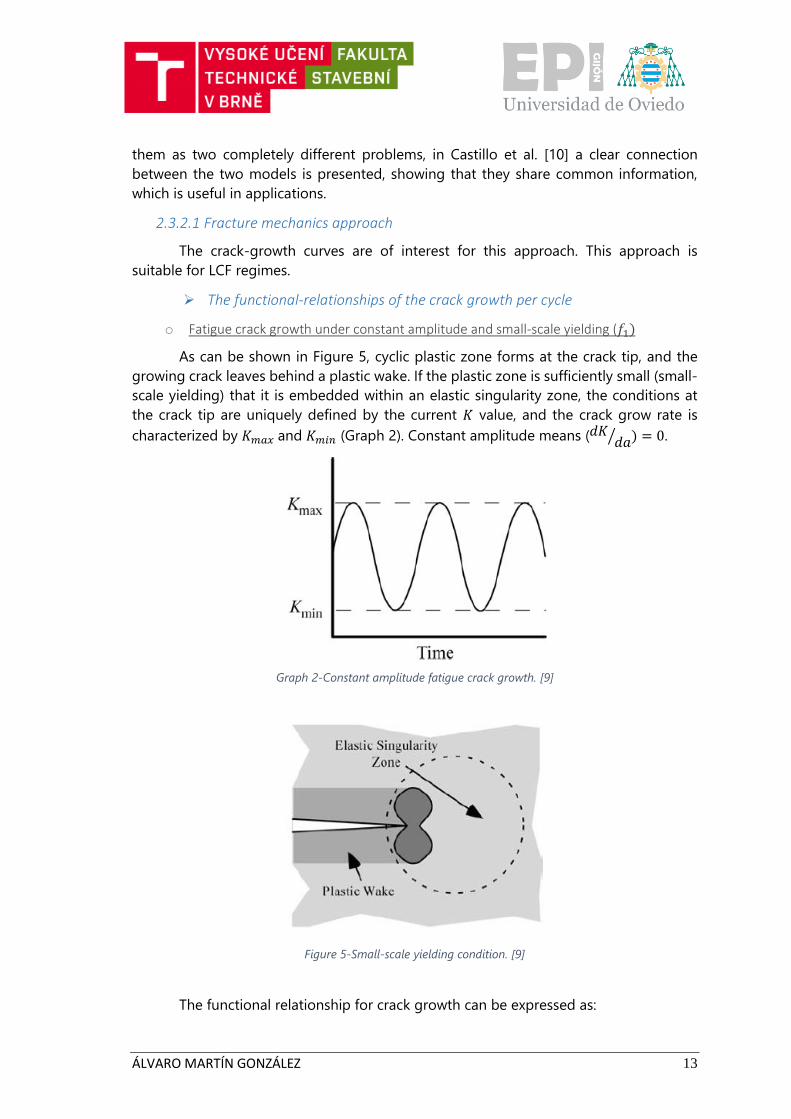
o Fatigue crack growth under constant amplitude and small-scale yielding (𝑓1)
As can be shown in Figure 5, cyclic plastic zone forms at the crack tip, and the
growing crack leaves behind a plastic wake. If the plastic zone is sufficiently small (small-
scale yielding) that it is embedded within an elastic singularity zone, the conditions at
the crack tip are uniquely defined by the current 𝐾 value, and the crack grow rate is
characterized by 𝐾𝑚𝑎𝑥 and 𝐾𝑚𝑖𝑛 (Graph 2). Constant amplitude means (𝑑𝐾𝑑𝑎⁄ ) = 0.
Graph 2-Constant amplitude fatigue crack growth. [9]
Figure 5-Small-scale yielding condition. [9]
The functional relationship for crack growth can be expressed as:
ÁLVARO MARTÍN GONZÁLEZ 14
𝑑𝑎
𝑑𝑁= 𝑓1(∆𝐾, 𝑅), (5)
where:
∆𝐾 = (𝐾𝑚𝑎𝑥 − 𝐾𝑚𝑖𝑛),
𝑅 =𝐾𝑚𝑖𝑛
𝐾𝑚𝑎𝑥 and
𝑑𝑎
𝑑𝑁=crack growth per cycle,
o Fatigue crack growth under variable amplitude (𝑓2)
If 𝐾𝑚𝑎𝑥 or 𝐾𝑚𝑖𝑛 varies during cyclic loading, the crack growth in a given cycle
depend on the loading history as well as the current values of 𝐾𝑚𝑖𝑛 and 𝐾𝑚𝑎𝑥.
The functional relationship for crack growth can be, then, expressed as:
𝑑𝑎
𝑑𝑁= 𝑓2(∆𝐾, 𝑅,ϗ) , (6)
where:
ϗ =history dependence, which results from prior plastic deformation.
Similitude of crack-tip conditions, which implies a unique relationship among 𝑑𝑎
𝑑𝑁,
∆𝐾, and 𝑅, is rigorously valid only for constant amplitude loading, as explained in the
previous item (2.2.1).
Variable amplitude fatigue analyses that account for prior loading history are
considerably more cumbersome than analyses that assume similitude. Therefore, the
latter type of analysis is desirable if the similitude assumption is justified. There are many
practical situations where such an assumption is reasonable. Such cases normally involve
cyclic loading at high 𝑅 ratios, where crack closure effects are negligible. Steel bridges,
for example, have high dead loads due to their own weight, which translates into high 𝑅
ratios. Also fatigue of welds that have not been stress relieved often obey similitude
because tensile residual stresses, which are static, increase the effective 𝑅 ratio.
o Fatigue crack growth under large-scale plasticity (𝑓3)
This is the second case where the similitude is violated since K no longer
characterizes the crack-tip conditions in such cases. Is the 𝐽 contour integral.
The functional relationship for crack growth can be, then, expressed as:
𝑑𝑎
𝑑𝑁= 𝑓3(∆𝐽, 𝑅), (7)
where:
∆𝐽=contour integral for cyclic loading, analogous to the 𝐽 integral for
monotonic loading.
However, Equation (7), as stated in (2.2.1), is only valid when no excessive
plasticity exits.
ÁLVARO MARTÍN GONZÁLEZ 15
➢ Stages of fatigue crack propagation and lifetime
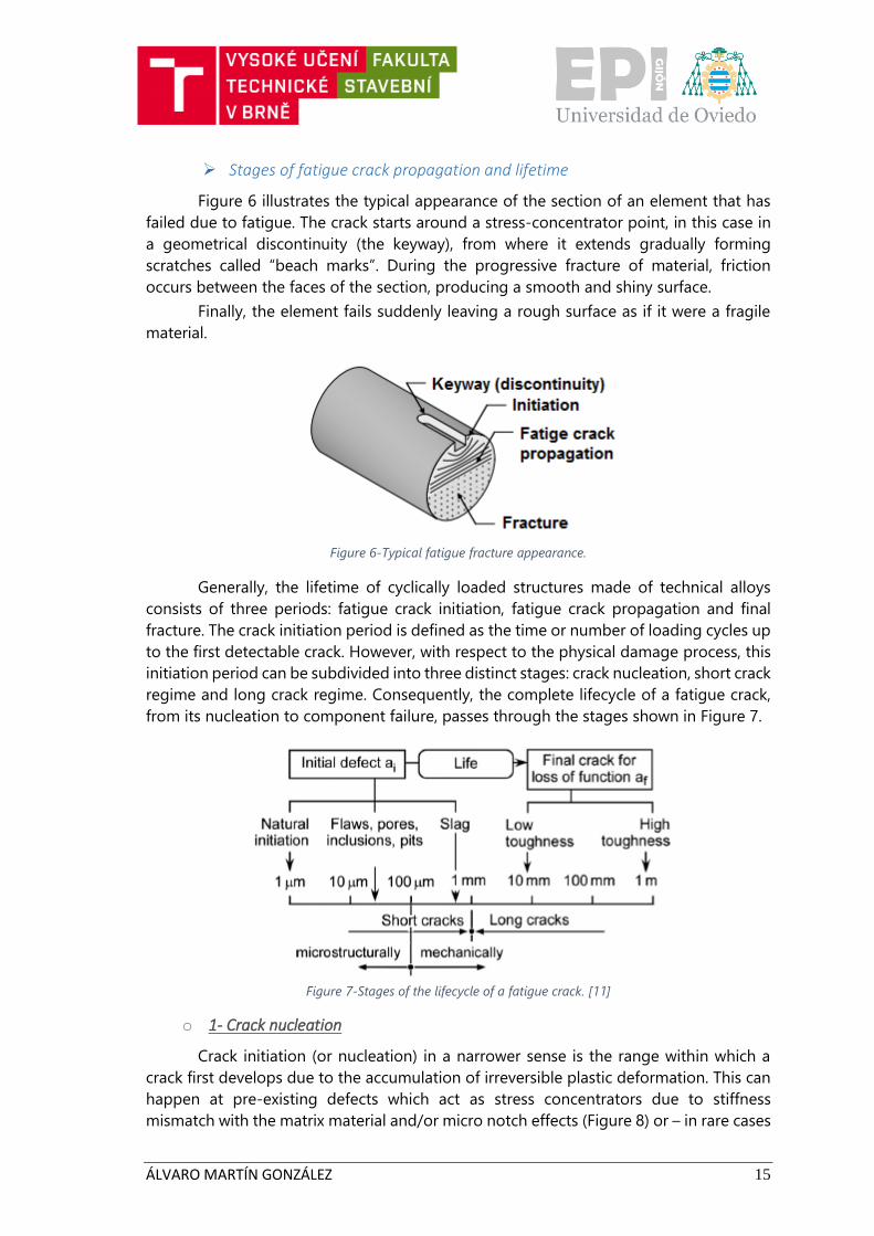
Figure 6 illustrates the typical appearance of the section of an element that has
failed due to fatigue. The crack starts around a stress-concentrator point, in this case in
a geometrical discontinuity (the keyway), from where it extends gradually forming
scratches called “beach marks”. During the progressive fracture of material, friction
occurs between the faces of the section, producing a smooth and shiny surface.
Finally, the element fails suddenly leaving a rough surface as if it were a fragile
material.
Figure 6-Typical fatigue fracture appearance.
Generally, the lifetime of cyclically loaded structures made of technical alloys
consists of three periods: fatigue crack initiation, fatigue crack propagation and final
fracture. The crack initiation period is defined as the time or number of loading cycles up
to the first detectable crack. However, with respect to the physical damage process, this
initiation period can be subdivided into three distinct stages: crack nucleation, short crack
regime and long crack regime. Consequently, the complete lifecycle of a fatigue crack,
from its nucleation to component failure, passes through the stages shown in Figure 7.
Figure 7-Stages of the lifecycle of a fatigue crack. [11]
o 1- Crack nucleation
Crack initiation (or nucleation) in a narrower sense is the range within which a
crack first develops due to the accumulation of irreversible plastic deformation. This can
happen at pre-existing defects which act as stress concentrators due to stiffness
mismatch with the matrix material and/or micro notch effects (Figure 8) or – in rare cases
ÁLVARO MARTÍN GONZÁLEZ 16
– at the defect free surface. The definition of the end of the initiation phase is a bit
academic because it is hard to define when exactly an original defect has become a crack.
The concepts of fracture mechanics similitude and a ∆𝐾 threshold break down near the
point of crack initiation.
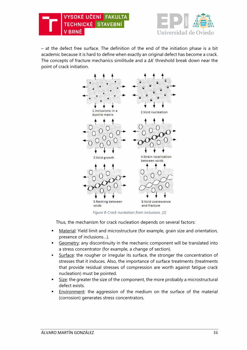
Figure 8-Crack nucleation from inclusions. [2]
Thus, the mechanism for crack nucleation depends on several factors:
▪ Material: Yield limit and microstructure (for example, grain size and orientation,
presence of inclusions…).
▪ Geometry: any discontinuity in the mechanic component will be translated into
a stress concentrator (for example, a change of section).
▪ Surface: the rougher or irregular its surface, the stronger the concentration of
stresses that it induces. Also, the importance of surface treatments (treatments
that provide residual stresses of compression are worth against fatigue crack
nucleation) must be pointed.
▪ Size: the greater the size of the component, the more probably a microstructural
defect exists.
▪ Environment: the aggression of the medium on the surface of the material
(corrosion) generates stress concentrators.
ÁLVARO MARTÍN GONZÁLEZ 17
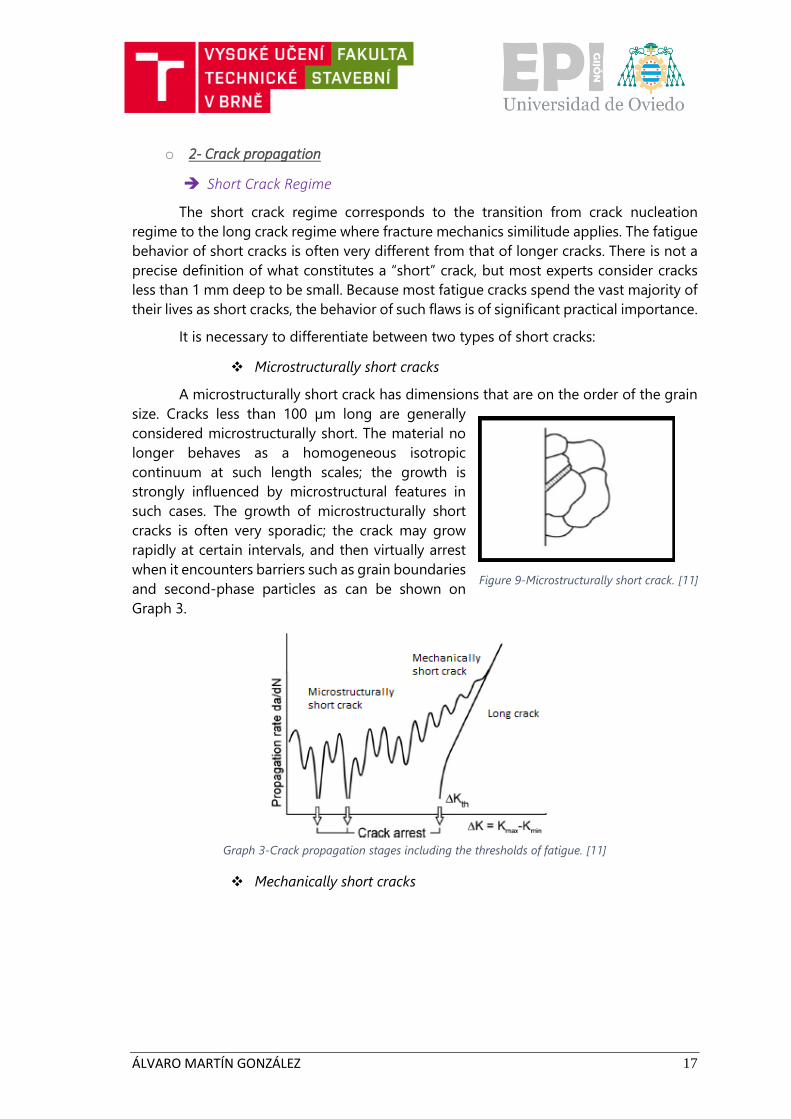
o 2- Crack propagation
➔ Short Crack Regime
The short crack regime corresponds to the transition from crack nucleation
regime to the long crack regime where fracture mechanics similitude applies. The fatigue
behavior of short cracks is often very different from that of longer cracks. There is not a
precise definition of what constitutes a “short” crack, but most experts consider cracks
less than 1 mm deep to be small. Because most fatigue cracks spend the vast majority of
their lives as short cracks, the behavior of such flaws is of significant practical importance.
It is necessary to differentiate between two types of short cracks:
❖ Microstructurally short cracks
A microstructurally short crack has dimensions that are on the order of the grain
size. Cracks less than 100 µm long are generally
considered microstructurally short. The material no
longer behaves as a homogeneous isotropic
continuum at such length scales; the growth is
strongly influenced by microstructural features in
such cases. The growth of microstructurally short
cracks is often very sporadic; the crack may grow
rapidly at certain intervals, and then virtually arrest
when it encounters barriers such as grain boundaries
and second-phase particles as can be shown on
Graph 3.
Graph 3-Crack propagation stages including the thresholds of fatigue. [11]
❖ Mechanically short cracks
Figure 9-Microstructurally short crack. [11]
ÁLVARO MARTÍN GONZÁLEZ 18
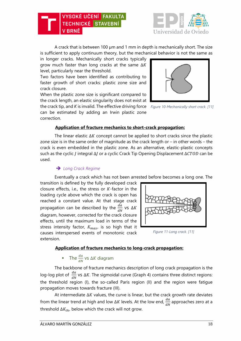
A crack that is between 100 µm and 1 mm in depth is mechanically short. The size
is sufficient to apply continuum theory, but the mechanical behavior is not the same as
in longer cracks. Mechanically short cracks typically
grow much faster than long cracks at the same ∆𝐾
level, particularly near the threshold.
Two factors have been identified as contributing to
faster growth of short cracks: plastic zone size and
crack closure.
When the plastic zone size is significant compared to
the crack length, an elastic singularity does not exist at
the crack tip, and K is invalid. The effective driving force
can be estimated by adding an Irwin plastic zone
correction.
Application of fracture mechanics to short-crack propagation:
The linear elastic ∆𝐾 concept cannot be applied to short cracks since the plastic
zone size is in the same order of magnitude as the crack length or – in other words – the
crack is even embedded in the plastic zone. As an alternative, elastic-plastic concepts
such as the cyclic 𝐽 integral ∆𝐽 or a cyclic Crack Tip Opening Displacement ∆𝐶𝑇𝑂𝐷 can be
used.
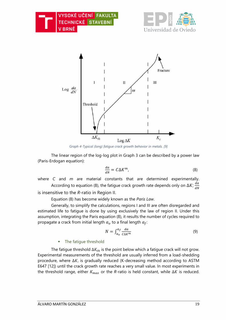
➔ Long Crack Regime
Eventually a crack which has not been arrested before becomes a long one. The
transition is defined by the fully developed crack
closure effects, i.e., the stress or 𝐾-factor in the
loading cycle above which the crack is open has
reached a constant value. At that stage crack
propagation can be described by the 𝑑𝑎
𝑑𝑁 vs ∆𝐾
diagram, however, corrected for the crack closure
effects, until the maximum load in terms of the
stress intensity factor, 𝐾𝑚𝑎𝑥, is so high that it
causes interspersed events of monotonic crack
extension.
Application of fracture mechanics to long-crack propagation:
▪ The 𝑑𝑎
𝑑𝑁 vs ∆𝐾 diagram
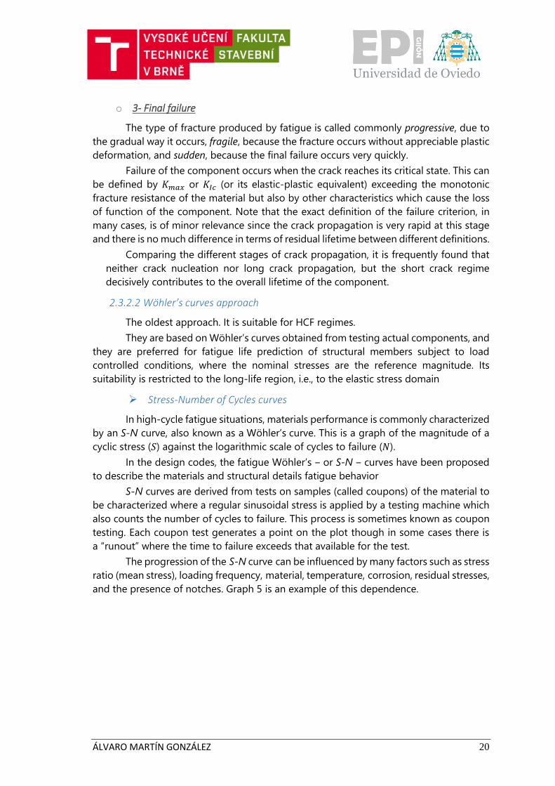
The backbone of fracture mechanics description of long crack propagation is the
log-log plot of 𝑑𝑎
𝑑𝑁 vs ∆𝐾. The sigmoidal curve (Graph 4) contains three distinct regions:
the threshold region (I), the so-called Paris region (II) and the region were fatigue
propagation moves towards fracture (III).
At intermediate ∆𝐾 values, the curve is linear, but the crack growth rate deviates
from the linear trend at high and low ∆𝐾 levels. At the low end, 𝑑𝑎
𝑑𝑁 approaches zero at a
threshold ∆𝐾𝑡ℎ, below which the crack will not grow.
Figure 10-Mechanically short crack. [11]
Figure 11-Long crack. [11]
ÁLVARO MARTÍN GONZÁLEZ 19
Graph 4-Typical (long) fatigue crack growth behavior in metals. [9]
The linear region of the log-log plot in Graph 3 can be described by a power law
(Paris-Erdogan equation):
𝑑𝑎
𝑑𝑁= 𝐶∆𝐾𝑚, (8)
where C and m are material constants that are determined experimentally.
According to equation (8), the fatigue crack growth rate depends only on ∆𝐾; 𝑑𝑎
𝑑𝑁
is insensitive to the R-ratio in Region II.
Equation (8) has become widely known as the Paris Law.
Generally, to simplify the calculations, regions I and III are often disregarded and
estimated life to fatigue is done by using exclusively the law of region II. Under this
assumption, integrating the Paris equation (8), it results the number of cycles required to
propagate a crack from initial length 𝑎𝑜 to a final length 𝑎𝑓:
𝑁 = ∫𝑑𝑎
𝐶∆𝐾𝑚
𝑎𝑓
𝑎𝑜 (9)
▪ The fatigue threshold
The fatigue threshold ∆𝐾𝑡ℎ is the point below which a fatigue crack will not grow.
Experimental measurements of the threshold are usually inferred from a load-shedding
procedure, where ∆𝐾, is gradually reduced (K-decreasing method according to ASTM
E647 [12]) until the crack growth rate reaches a very small value. In most experiments in
the threshold range, either 𝐾𝑚𝑎𝑥 or the R-ratio is held constant, while ∆𝐾 is reduced.
ÁLVARO MARTÍN GONZÁLEZ 20
o 3- Final failure
The type of fracture produced by fatigue is called commonly progressive, due to
the gradual way it occurs, fragile, because the fracture occurs without appreciable plastic
deformation, and sudden, because the final failure occurs very quickly.
Failure of the component occurs when the crack reaches its critical state. This can
be defined by 𝐾𝑚𝑎𝑥 or 𝐾𝐼𝑐 (or its elastic-plastic equivalent) exceeding the monotonic
fracture resistance of the material but also by other characteristics which cause the loss
of function of the component. Note that the exact definition of the failure criterion, in
many cases, is of minor relevance since the crack propagation is very rapid at this stage
and there is no much difference in terms of residual lifetime between different definitions.
Comparing the different stages of crack propagation, it is frequently found that
neither crack nucleation nor long crack propagation, but the short crack regime
decisively contributes to the overall lifetime of the component.
2.3.2.2 Wöhler’s curves approach
The oldest approach. It is suitable for HCF regimes.
They are based on Wöhler’s curves obtained from testing actual components, and
they are preferred for fatigue life prediction of structural members subject to load
controlled conditions, where the nominal stresses are the reference magnitude. Its
suitability is restricted to the long-life region, i.e., to the elastic stress domain
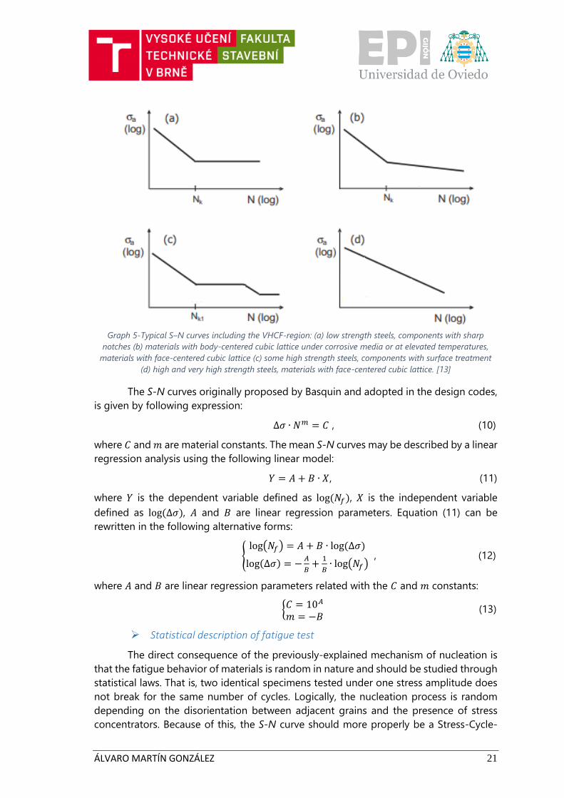
➢ Stress-Number of Cycles curves
In high-cycle fatigue situations, materials performance is commonly characterized
by an S-N curve, also known as a Wöhler’s curve. This is a graph of the magnitude of a
cyclic stress (𝑆) against the logarithmic scale of cycles to failure (𝑁).
In the design codes, the fatigue Wöhler’s ‒ or S-N ‒ curves have been proposed
to describe the materials and structural details fatigue behavior
S-N curves are derived from tests on samples (called coupons) of the material to
be characterized where a regular sinusoidal stress is applied by a testing machine which
also counts the number of cycles to failure. This process is sometimes known as coupon
testing. Each coupon test generates a point on the plot though in some cases there is
a “runout” where the time to failure exceeds that available for the test.
The progression of the S-N curve can be influenced by many factors such as stress
ratio (mean stress), loading frequency, material, temperature, corrosion, residual stresses,
and the presence of notches. Graph 5 is an example of this dependence.
ÁLVARO MARTÍN GONZÁLEZ 21
Graph 5-Typical S–N curves including the VHCF-region: (a) low strength steels, components with sharp
notches (b) materials with body-centered cubic lattice under corrosive media or at elevated temperatures,
materials with face-centered cubic lattice (c) some high strength steels, components with surface treatment
(d) high and very high strength steels, materials with face-centered cubic lattice. [13]
The S-N curves originally proposed by Basquin and adopted in the design codes,
is given by following expression:
∆𝜎 ∙ 𝑁𝑚 = 𝐶 , (10)
where 𝐶 and 𝑚 are material constants. The mean S-N curves may be described by a linear
regression analysis using the following linear model:
𝑌 = 𝐴 + 𝐵 ∙ 𝑋 , (11)
where 𝑌 is the dependent variable defined as log (𝑁𝑓), 𝑋 is the independent variable
defined as log (∆𝜎), 𝐴 and 𝐵 are linear regression parameters. Equation (11) can be
rewritten in the following alternative forms:
{log(𝑁𝑓) = 𝐴 + 𝐵 ∙ log (∆𝜎)
log(∆𝜎) = −𝐴
𝐵+
1
𝐵∙ log(𝑁𝑓)
, (12)
where 𝐴 and 𝐵 are linear regression parameters related with the 𝐶 and 𝑚 constants:
{𝐶 = 10𝐴
𝑚 = −𝐵 (13)
➢ Statistical description of fatigue test
The direct consequence of the previously-explained mechanism of nucleation is
that the fatigue behavior of materials is random in nature and should be studied through
statistical laws. That is, two identical specimens tested under one stress amplitude does
not break for the same number of cycles. Logically, the nucleation process is random
depending on the disorientation between adjacent grains and the presence of stress
concentrators. Because of this, the S-N curve should more properly be a Stress-Cycle-
ÁLVARO MARTÍN GONZÁLEZ 22
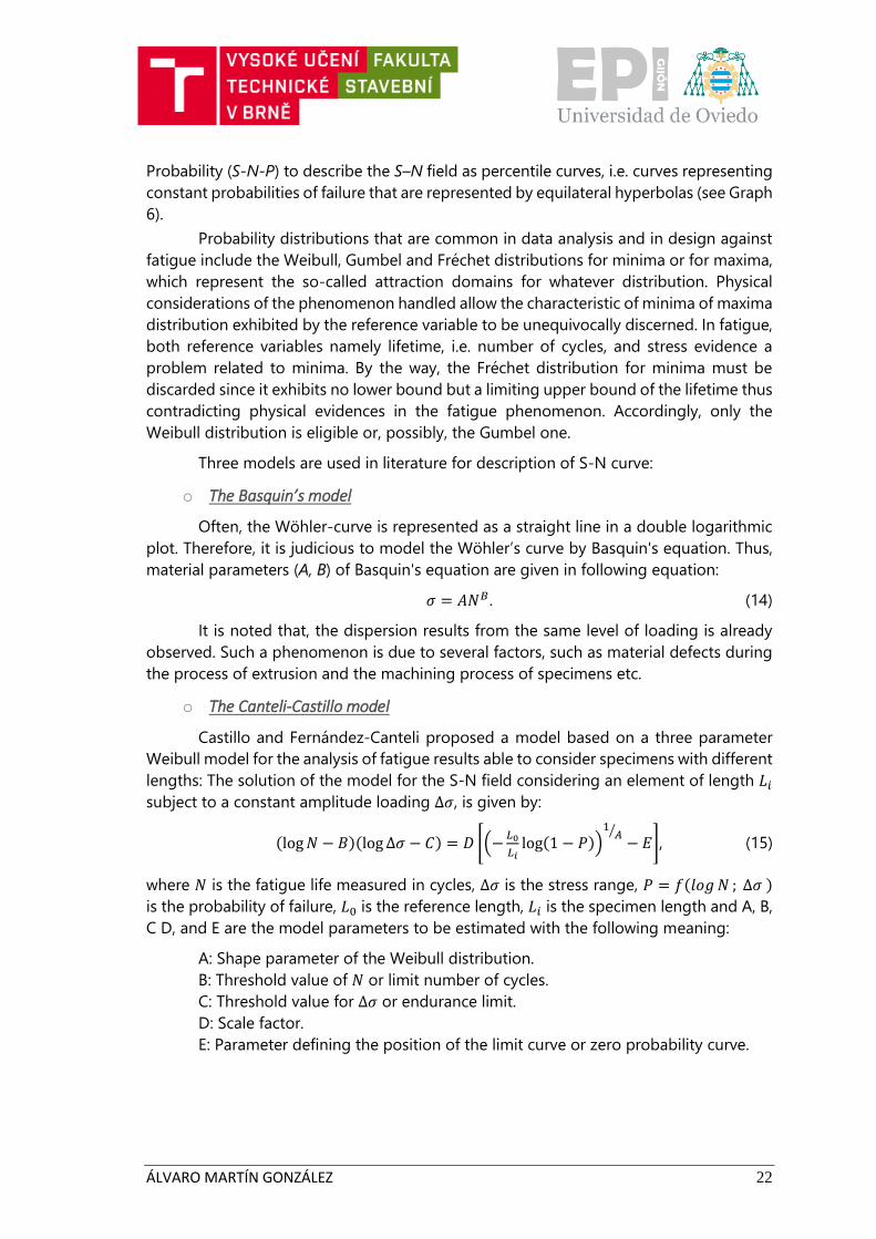
Probability (S-N-P) to describe the S–N field as percentile curves, i.e. curves representing
constant probabilities of failure that are represented by equilateral hyperbolas (see Graph
6).
Probability distributions that are common in data analysis and in design against
fatigue include the Weibull, Gumbel and Fréchet distributions for minima or for maxima,
which represent the so-called attraction domains for whatever distribution. Physical
considerations of the phenomenon handled allow the characteristic of minima of maxima
distribution exhibited by the reference variable to be unequivocally discerned. In fatigue,
both reference variables namely lifetime, i.e. number of cycles, and stress evidence a
problem related to minima. By the way, the Fréchet distribution for minima must be
discarded since it exhibits no lower bound but a limiting upper bound of the lifetime thus
contradicting physical evidences in the fatigue phenomenon. Accordingly, only the
Weibull distribution is eligible or, possibly, the Gumbel one.
Three models are used in literature for description of S-N curve:
o The Basquin’s model
Often, the Wöhler-curve is represented as a straight line in a double logarithmic
plot. Therefore, it is judicious to model the Wöhler’s curve by Basquin's equation. Thus,
material parameters (A, B) of Basquin's equation are given in following equation:
𝜎 = 𝐴𝑁𝐵. (14)
It is noted that, the dispersion results from the same level of loading is already
observed. Such a phenomenon is due to several factors, such as material defects during
the process of extrusion and the machining process of specimens etc.
o The Canteli-Castillo model
Castillo and Fernández-Canteli proposed a model based on a three parameter
Weibull model for the analysis of fatigue results able to consider specimens with different
lengths: The solution of the model for the S-N field considering an element of length 𝐿𝑖
subject to a constant amplitude loading ∆𝜎, is given by:
(log 𝑁 − 𝐵)(log ∆𝜎 − 𝐶) = 𝐷 [(−𝐿0
𝐿𝑖log(1 − 𝑃))
1𝐴⁄
− 𝐸], (15)
where 𝑁 is the fatigue life measured in cycles, ∆𝜎 is the stress range, 𝑃 = 𝑓(𝑙𝑜𝑔 𝑁 ; ∆𝜎 )
is the probability of failure, 𝐿0 is the reference length, 𝐿𝑖 is the specimen length and A, B,
C D, and E are the model parameters to be estimated with the following meaning:
A: Shape parameter of the Weibull distribution.
B: Threshold value of 𝑁 or limit number of cycles.
C: Threshold value for ∆𝜎 or endurance limit.
D: Scale factor.
E: Parameter defining the position of the limit curve or zero probability curve.
ÁLVARO MARTÍN GONZÁLEZ 23
Graph 6-S-N field with percentile curves representing the same probability of failure. [14]
The estimation of the parameters follows in two steps. In the first step B and C
are estimated while the rest of the parameters, i.e., A, D and E are calculated in a second
stage. Different mathematical methods have been proposed by Castillo et al. [15], [16],
[17].
o The Kohout-Věchet model
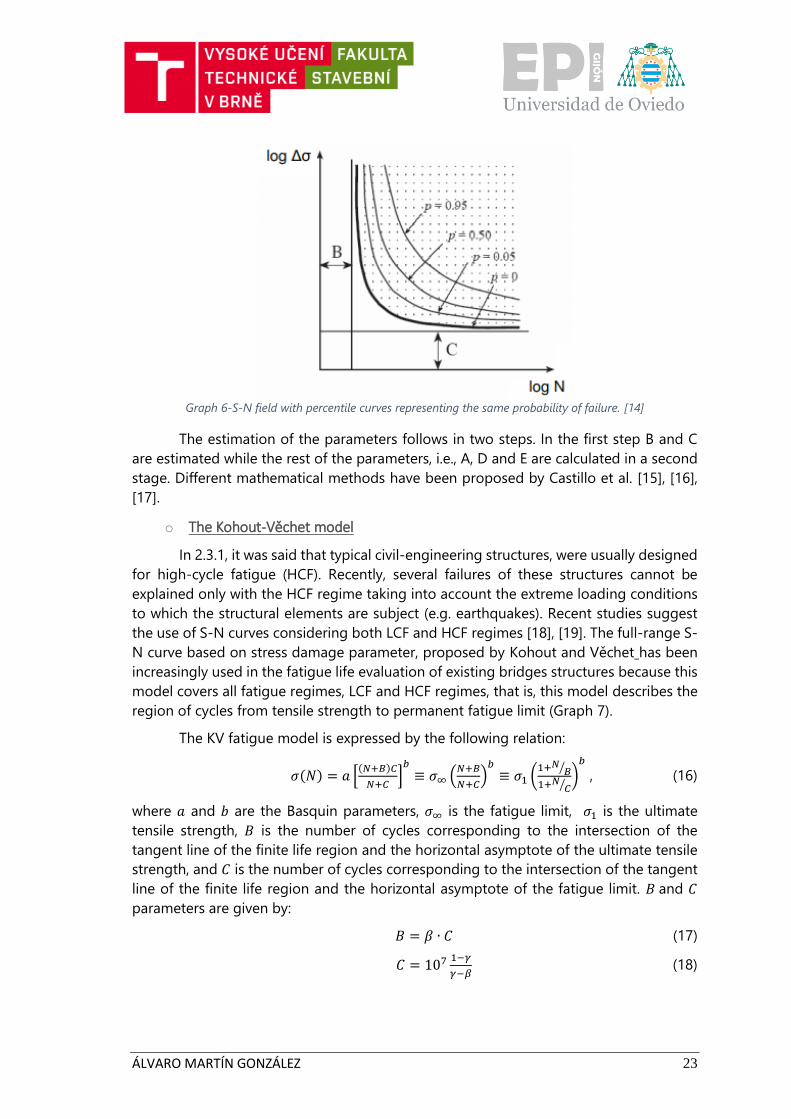
In 2.3.1, it was said that typical civil-engineering structures, were usually designed
for high-cycle fatigue (HCF). Recently, several failures of these structures cannot be
explained only with the HCF regime taking into account the extreme loading conditions
to which the structural elements are subject (e.g. earthquakes). Recent studies suggest
the use of S-N curves considering both LCF and HCF regimes [18], [19]. The full-range S-
N curve based on stress damage parameter, proposed by Kohout and Věchet has been
increasingly used in the fatigue life evaluation of existing bridges structures because this
model covers all fatigue regimes, LCF and HCF regimes, that is, this model describes the
region of cycles from tensile strength to permanent fatigue limit (Graph 7).
The KV fatigue model is expressed by the following relation:
𝜎(𝑁) = 𝑎 [(𝑁+𝐵)𝐶
𝑁+𝐶]
𝑏≡ 𝜎∞ (
𝑁+𝐵
𝑁+𝐶)
𝑏≡ 𝜎1 (
1+𝑁𝐵⁄
1+𝑁𝐶⁄
)𝑏
, (16)
where 𝑎 and 𝑏 are the Basquin parameters, 𝜎∞ is the fatigue limit, 𝜎1 is the ultimate
tensile strength, 𝐵 is the number of cycles corresponding to the intersection of the
tangent line of the finite life region and the horizontal asymptote of the ultimate tensile
strength, and 𝐶 is the number of cycles corresponding to the intersection of the tangent
line of the finite life region and the horizontal asymptote of the fatigue limit. 𝐵 and 𝐶
parameters are given by:
𝐵 = 𝛽 ∙ 𝐶 (17)
𝐶 = 107 1−𝛾
𝛾−𝛽 (18)
ÁLVARO MARTÍN GONZÁLEZ 24
Graph 7-Schematic representation of the Kohout-Věchet S-N curve. [20]
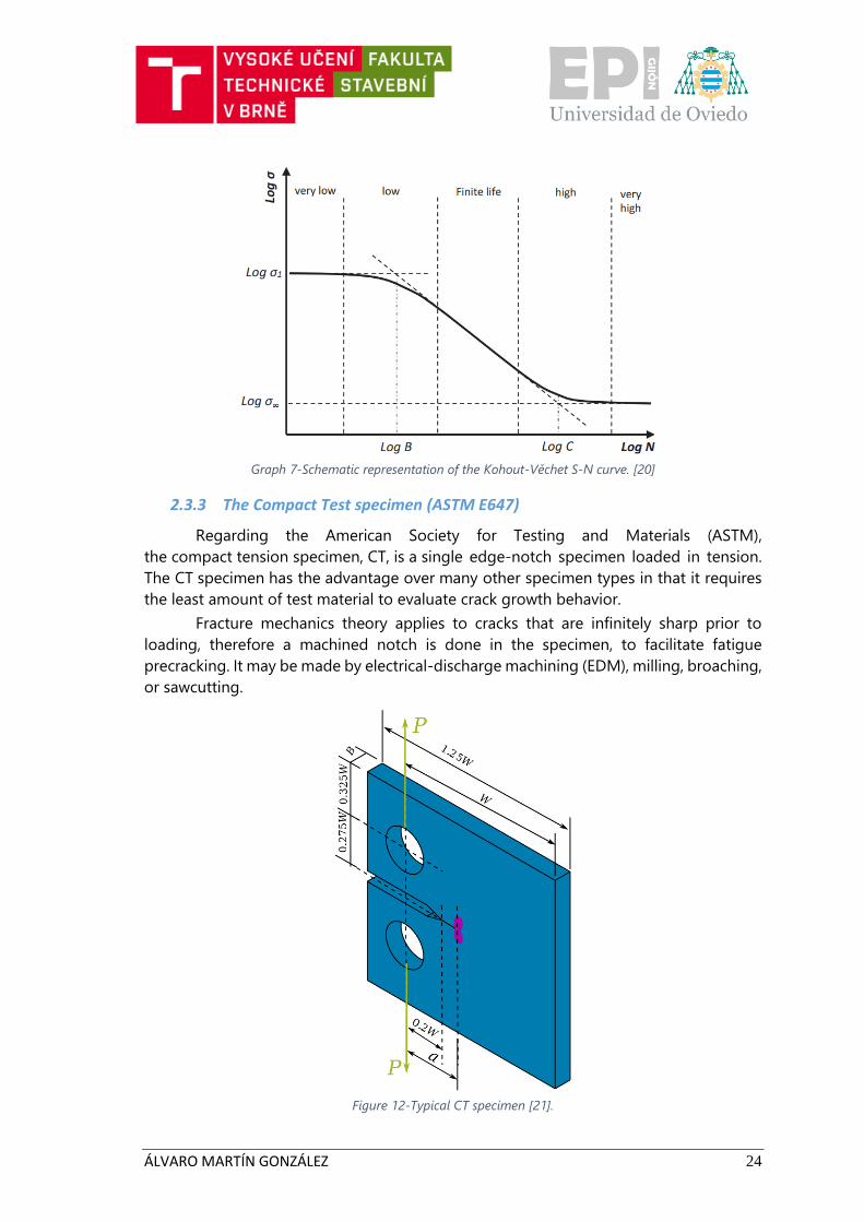
2.3.3 The Compact Test specimen (ASTM E647)
Regarding the American Society for Testing and Materials (ASTM),
the compact tension specimen, CT, is a single edge-notch specimen loaded in tension.
The CT specimen has the advantage over many other specimen types in that it requires
the least amount of test material to evaluate crack growth behavior.
Fracture mechanics theory applies to cracks that are infinitely sharp prior to
loading, therefore a machined notch is done in the specimen, to facilitate fatigue
precracking. It may be made by electrical-discharge machining (EDM), milling, broaching,
or sawcutting.
Figure 12-Typical CT specimen [21].
ÁLVARO MARTÍN GONZÁLEZ 25
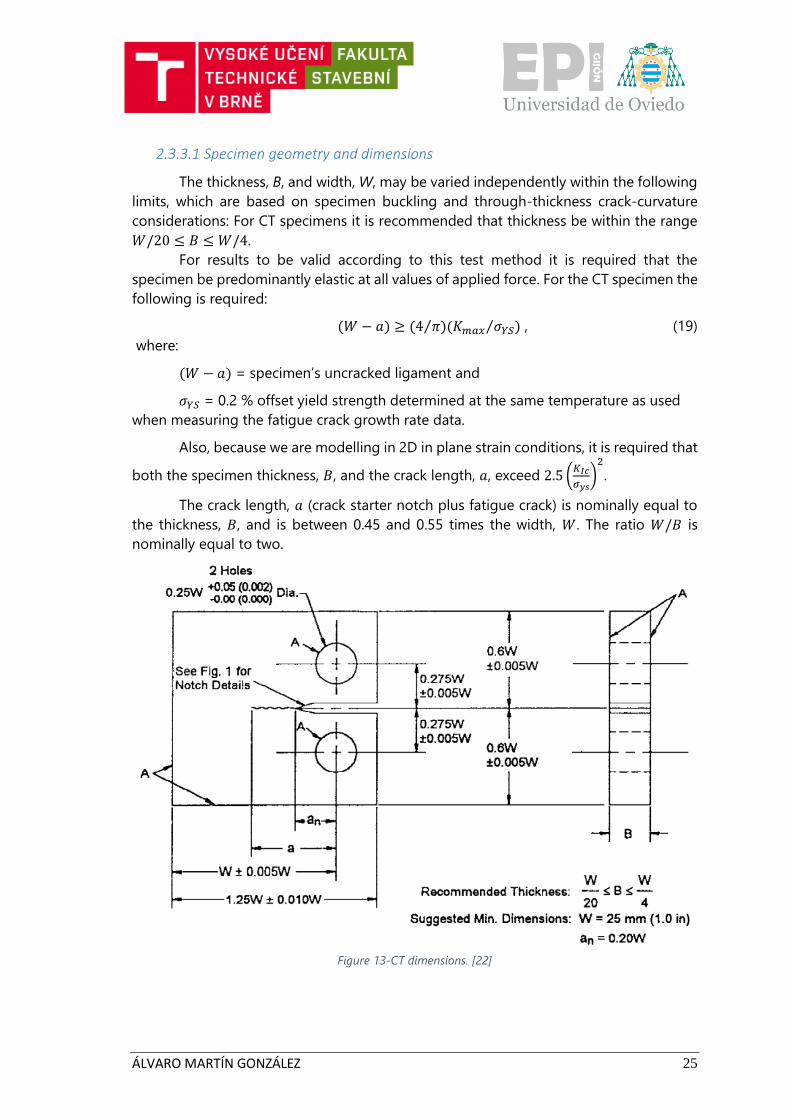
2.3.3.1 Specimen geometry and dimensions
The thickness, B, and width, W, may be varied independently within the following
limits, which are based on specimen buckling and through-thickness crack-curvature
considerations: For CT specimens it is recommended that thickness be within the range
𝑊/20 ≤ 𝐵 ≤ 𝑊/4.
For results to be valid according to this test method it is required that the
specimen be predominantly elastic at all values of applied force. For the CT specimen the
following is required:
(𝑊 − 𝑎) ≥ (4 𝜋)(𝐾𝑚𝑎𝑥 𝜎𝑌𝑆)⁄⁄ , (19)
where:
(𝑊 − 𝑎) = specimen’s uncracked ligament and
𝜎𝑌𝑆 = 0.2 % offset yield strength determined at the same temperature as used
when measuring the fatigue crack growth rate data.
Also, because we are modelling in 2D in plane strain conditions, it is required that
both the specimen thickness, 𝐵, and the crack length, 𝑎, exceed 2.5 (𝐾𝐼𝑐
𝜎𝑦𝑠)
2
.
The crack length, 𝑎 (crack starter notch plus fatigue crack) is nominally equal to
the thickness, 𝐵, and is between 0.45 and 0.55 times the width, 𝑊. The ratio 𝑊/𝐵 is
nominally equal to two.
Figure 13-CT dimensions. [22]
ÁLVARO MARTÍN GONZÁLEZ 26
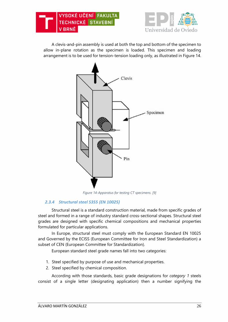
A clevis-and-pin assembly is used at both the top and bottom of the specimen to
allow in-plane rotation as the specimen is loaded. This specimen and loading
arrangement is to be used for tension-tension loading only, as illustrated in Figure 14.
Figure 14-Apparatus for testing CT specimens. [9]
2.3.4 Structural steel S355 (EN 10025)
Structural steel is a standard construction material, made from specific grades of
steel and formed in a range of industry standard cross-sectional shapes. Structural steel
grades are designed with specific chemical compositions and mechanical properties
formulated for particular applications.
In Europe, structural steel must comply with the European Standard EN 10025
and Governed by the ECISS (European Committee for Iron and Steel Standardization) a
subset of CEN (European Committee for Standardization).
European standard steel grade names fall into two categories:
1. Steel specified by purpose of use and mechanical properties.
2. Steel specified by chemical composition.
According with those standards, basic grade designations for category 1 steels
consist of a single letter (designating application) then a number signifying the
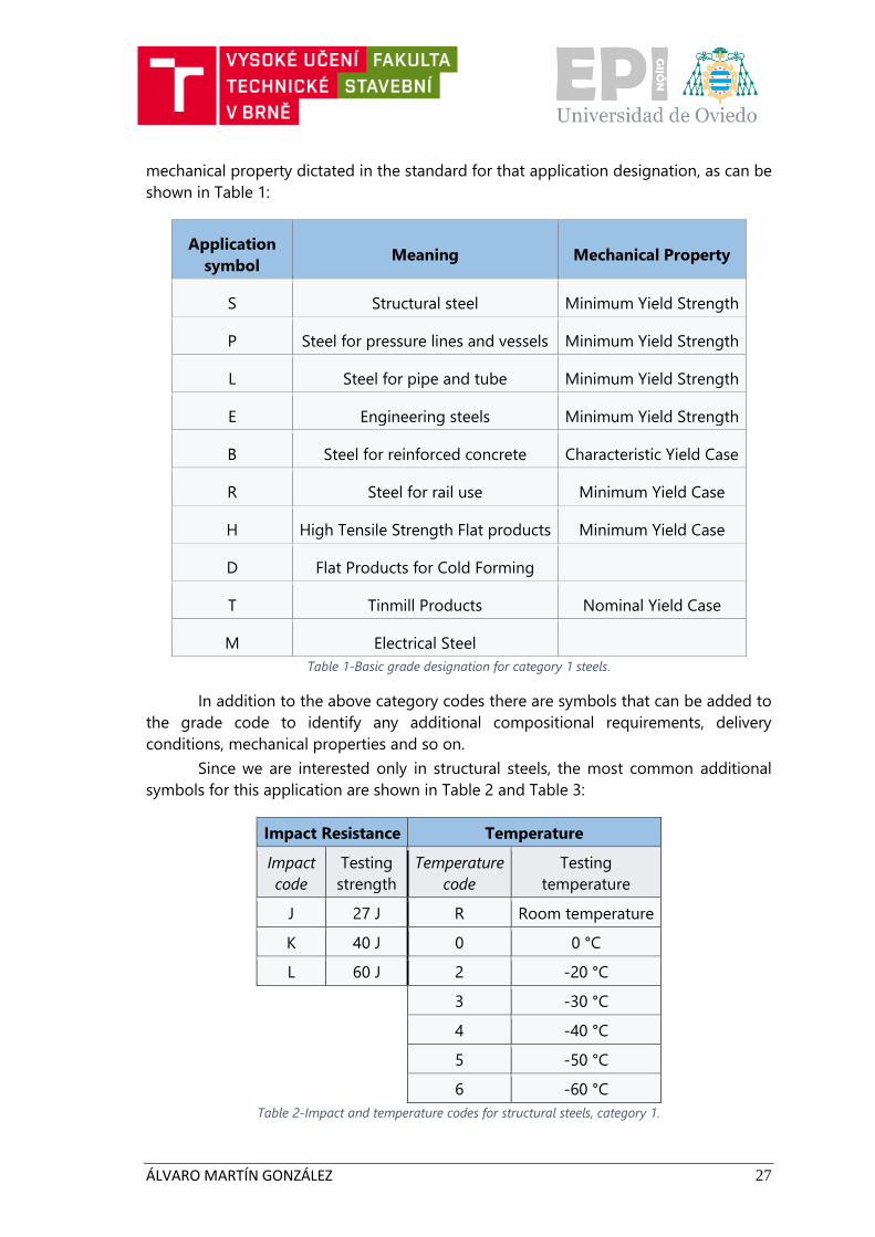
ÁLVARO MARTÍN GONZÁLEZ 27
mechanical property dictated in the standard for that application designation, as can be
shown in Table 1:
Application
symbol Meaning Mechanical Property
S Structural steel Minimum Yield Strength
P Steel for pressure lines and vessels Minimum Yield Strength
L Steel for pipe and tube Minimum Yield Strength
E Engineering steels Minimum Yield Strength
B Steel for reinforced concrete Characteristic Yield Case
R Steel for rail use Minimum Yield Case
H High Tensile Strength Flat products Minimum Yield Case
D Flat Products for Cold Forming
T Tinmill Products Nominal Yield Case
M Electrical Steel
Table 1-Basic grade designation for category 1 steels.
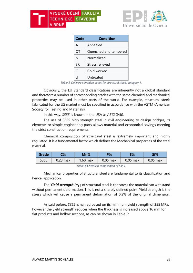
In addition to the above category codes there are symbols that can be added to
the grade code to identify any additional compositional requirements, delivery
conditions, mechanical properties and so on.
Since we are interested only in structural steels, the most common additional
symbols for this application are shown in Table 2 and Table 3:
Impact Resistance Temperature
Impact
code
Testing
strength
Temperature
code
Testing
temperature
J 27 J R Room temperature
K 40 J 0 0 °C
L 60 J 2 -20 °C
3 -30 °C
4 -40 °C
5 -50 °C
6 -60 °C
Table 2-Impact and temperature codes for structural steels, category 1.
ÁLVARO MARTÍN GONZÁLEZ 28
Code Condition
A Annealed
QT Quenched and tempered
N Normalized
SR Stress relieved
C Cold worked
U Untreated
Table 3-Delivery condition codes for structural steels, category 1.
Obviously, the EU Standard classifications are inherently not a global standard
and therefore a number of corresponding grades with the same chemical and mechanical
properties may be used in other parts of the world. For example, structural steels
fabricated for the US market must be specified in accordance with the ASTM (American
Society for Testing and Materials).
In this way, S355 is known in the USA as A572Gr50.
The use of S355 high strength steel in civil engineering to design bridges, its
elements or simple engineering parts allows material and economical savings meeting
the strict construction requirements.
Chemical composition of structural steel is extremely important and highly
regulated. It is a fundamental factor which defines the Mechanical properties of the steel
material.
Grade C% Mn% P% S% Si%
S355 0.23 max 1.60 max 0.05 max 0.05 max 0.05 max
Table 4-Chemical composition of S355.
Mechanical properties of structural steel are fundamental to its classification and
hence, application.
The Yield strength (𝝈𝒀) of structural steel is the stress the material can withstand
without permanent deformation. This is not a sharply defined point. Yield strength is the
stress which will cause a permanent deformation of 0.2% of the original dimension.
As said before, S355 is named based on its minimum yield strength of 355 MPa,
however the yield strength reduces when the thickness is increased above 16 mm for
flat products and hollow sections, as can be shown in Table 5:
ÁLVARO MARTÍN GONZÁLEZ 29
Thickness, t [mm] Yield Strength [MPa]
Up to 16
355
16 < t ≤ 40
345
40 < t ≤ 63
335
63 < t ≤ 80
325
80 < t ≤ 100
315
100 < t ≤ 150 295
Table 5-Yield Strength for S355.
The Ultimate Tensile Strength (UTS) of Structural steel relates to the point of
maximum stress that the material can withstand.
S355 ultimate tensile strength ranges also varies based on thickness, as shown in
Table 6:
Thickness, t [mm] Tensile Strength [MPa]
Up to 3
510 to 680
3 < t ≤ 100 470 to 630
100 < t ≤ 150 450 to 600
Table 6-Ultimate strength for S355.
The Density (ρ) of S355 is 7850 kg/m3 like all other mild steel.
Therefore, all the above-mentioned properties vary depending on the grade of
the S355 steel and in the thickness. In this thesis, two different grades will be evaluated:
- S355 J2: Testing strength of 27J at a temperature of -20 ºC.
Steel grade
C max.
%
Mn max.
%
Si max.
%
P max.
%
S max.
%
N max.
%
Cu max.
%
Other max.
%
S355 J2 0,22 1.60 0.55 0,030 0,030 - 0,55 -
Table 7-Chemical composition in percentage by weight of steel grade S355 J2 according to EN 10025-2:2004
standard.
- S355 J0: Testing strength of 27J at room temperature (20 ºC).
Steel grade
C max.
%
Mn max.
%
Si max.
%
P max.
%
S max.
%
N max.
%
Cu max.
%
Other max.
%
S355 J0 0,22 1.60 0.55 0,035 0,035 0.012 0,55 -
Table 8-Chemical composition in percentage by weight of steel grade S355 J0 according to EN 10025-2:2004
standard.
ÁLVARO MARTÍN GONZÁLEZ 30
3. AIM OF THESIS
The objective of this thesis is to measure, evaluate and compare fatigue properties
of different S355 steels. Fatigue and Fracture Mechanics properties such as SIF and T-
stress will be also considered.
To this end, the Finite Element model of compact tension is prepared and the
calibration curves are calculated.
The S-N curves of two standard S355 steel grades (“J0” and “J2”) are evaluated by
Basquin’s model and the crack propagation rate curves are evaluated by compact tension
specimens. The stress intensity factor and the 𝑇-stress in the crack tip are also measured.
Those experimental data from IPM and numerical data obtained from FEM
software are evaluated and compared with literature.
ÁLVARO MARTÍN GONZÁLEZ 31
4. NUMERICAL MODELING IN ANSYS
Software ANSYS is used to obtain numerically values for the K factor and 𝑇-stress.
It is recommended to see Appendix 10.5 “APPENDIX V - Macro for the CT
specimen” to check the modeling. Further information about the commands used, can be
found in [30].
4.1 Prior set up
Prior to start with the modeling in the preprocessor, some adjustments should be
done: clean the setup area, set the title of the file, order the numeration of key points,
lines and areas, set the coordinate system, clear variables, stablish the color of the
elements to be displayed and apply 2D, plane strain conditions.
4.2 Pre-processor
4.2.1 Specimen
Once in the pre-processor, it is time to set the parameters that are going to lead
the analysis.
As previously said (2.3.3), the specimen chosen is the CT one. The characteristic
dimensions are shown in Figure 13.
Because 2D analysis plane strain is performed, the parameters to be defined, as
can be shown, are W and a. W is the specimen width and a is the crack length.
W is set as 50 mm while a depends on the 𝑎/𝑊 ratio, that is stablished from 0.02
to 0.90 in steps of 0.02.
4.2.2 Element type
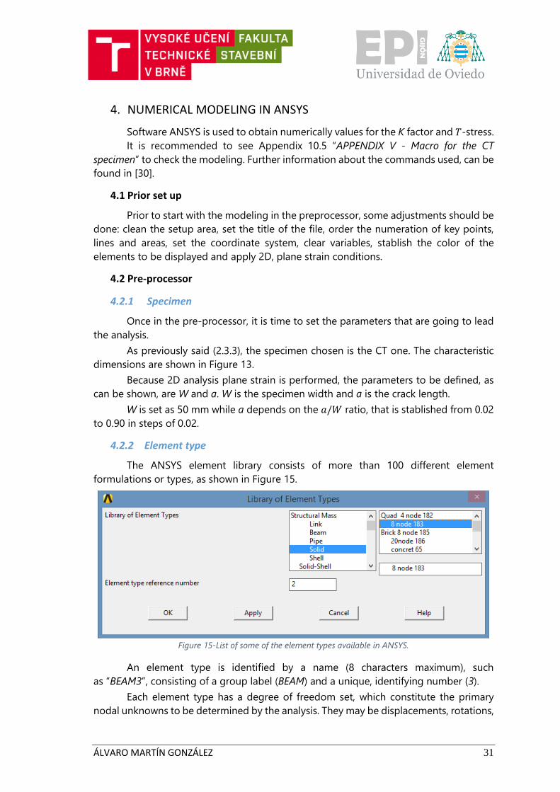
The ANSYS element library consists of more than 100 different element
formulations or types, as shown in Figure 15.
Figure 15-List of some of the element types available in ANSYS.
An element type is identified by a name (8 characters maximum), such
as “BEAM3”, consisting of a group label (BEAM) and a unique, identifying number (3).
Each element type has a degree of freedom set, which constitute the primary
nodal unknowns to be determined by the analysis. They may be displacements, rotations,
ÁLVARO MARTÍN GONZÁLEZ 32
temperatures, pressures, voltages, etc. Derived results, such as stresses, heat flows, etc.,
are computed from these degree of freedom results. Degrees of freedom are not defined
on the nodes explicitly by the user, but rather are implied by the element types attached
to them. The choice of element types is therefore, an important one in any ANSYS
analysis.
For this modeling, element “PLANE82” (in Figure 15, selected as “Solid”> “8 node
183”) is chosen because it is required, for the calculation of the stress intensity factor, a
shift of one node to 1/4 of the element length.
“PLANE82” provides more accurate results for mixed (quadrilateral-triangular)
automatic meshes and can tolerate irregular shapes without as much loss of accuracy.
The 8-node elements have compatible displacement shapes and are well suited to model
curved boundaries.
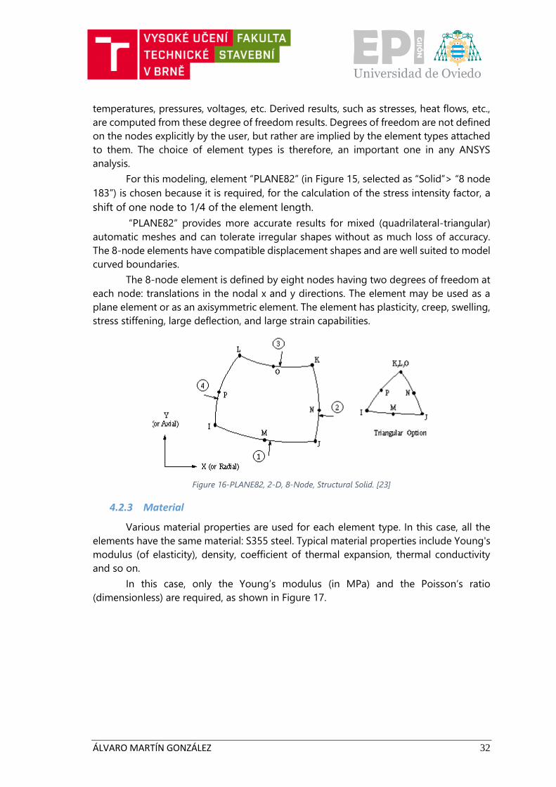
The 8-node element is defined by eight nodes having two degrees of freedom at
each node: translations in the nodal x and y directions. The element may be used as a
plane element or as an axisymmetric element. The element has plasticity, creep, swelling,
stress stiffening, large deflection, and large strain capabilities.
Figure 16-PLANE82, 2-D, 8-Node, Structural Solid. [23]
4.2.3 Material
Various material properties are used for each element type. In this case, all the
elements have the same material: S355 steel. Typical material properties include Young's
modulus (of elasticity), density, coefficient of thermal expansion, thermal conductivity
and so on.
In this case, only the Young’s modulus (in MPa) and the Poisson’s ratio
(dimensionless) are required, as shown in Figure 17.
ÁLVARO MARTÍN GONZÁLEZ 33
Figure 17-Linear isotropic properties for steel. Young’s modulus (EX) [MPa] and Poisson’s number (NUXY) [-].
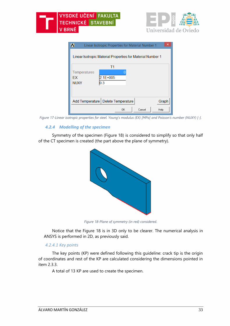
4.2.4 Modelling of the specimen
Symmetry of the specimen (Figure 18) is considered to simplify so that only half
of the CT specimen is created (the part above the plane of symmetry).
Figure 18-Plane of symmetry (in red) considered.
Notice that the Figure 18 is in 3D only to be clearer. The numerical analysis in
ANSYS is performed in 2D, as previously said.
4.2.4.1 Key points
The key points (KP) were defined following this guideline: crack tip is the origin
of coordinates and rest of the KP are calculated considering the dimensions pointed in
item 2.3.3.
A total of 13 KP are used to create the specimen.
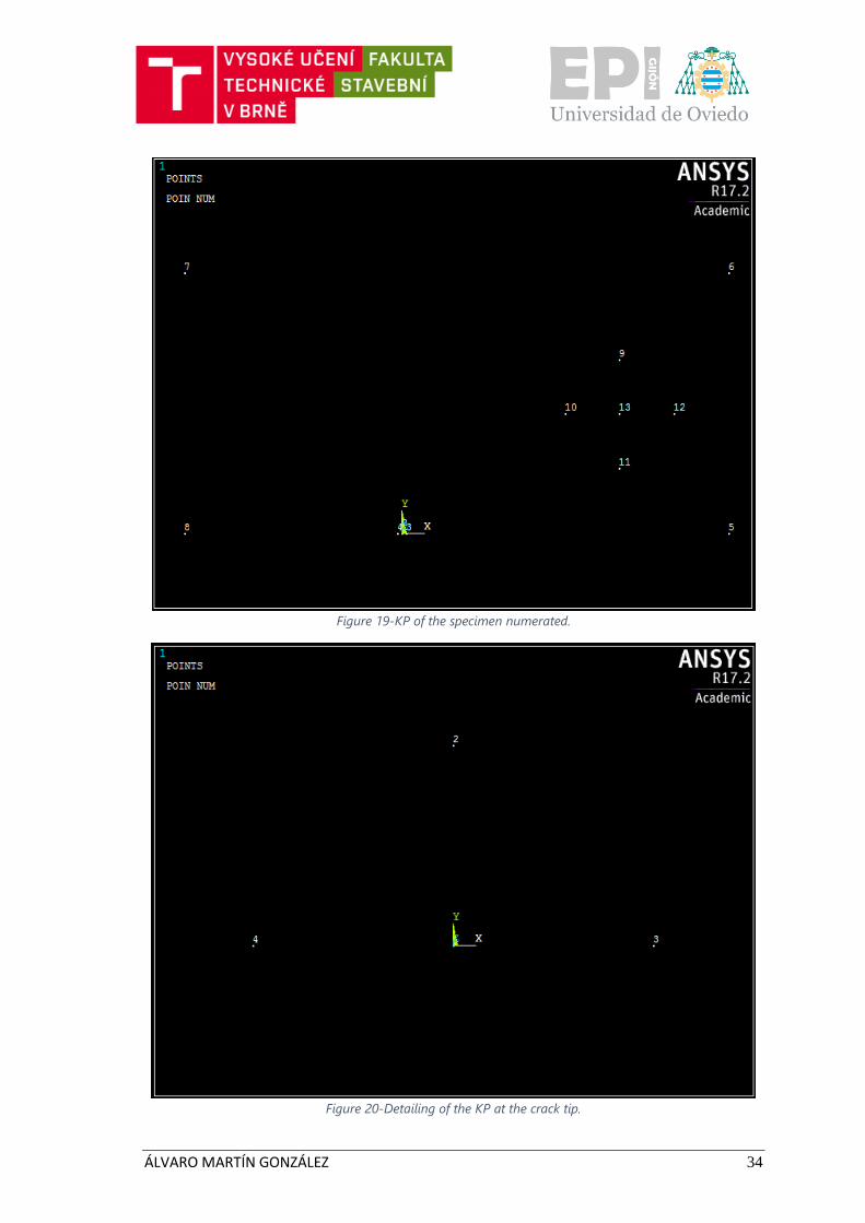
ÁLVARO MARTÍN GONZÁLEZ 34
Figure 19-KP of the specimen numerated.
Figure 20-Detailing of the KP at the crack tip.
ÁLVARO MARTÍN GONZÁLEZ 35
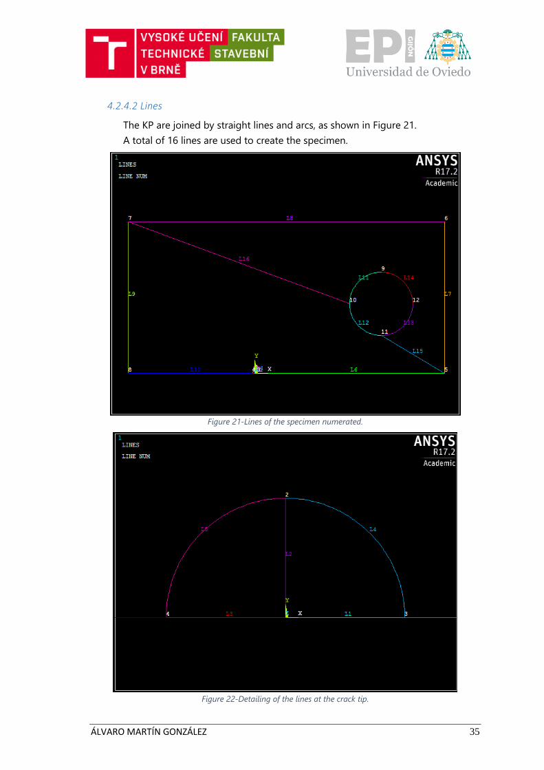
4.2.4.2 Lines
The KP are joined by straight lines and arcs, as shown in Figure 21.
A total of 16 lines are used to create the specimen.
Figure 21-Lines of the specimen numerated.
Figure 22-Detailing of the lines at the crack tip.
ÁLVARO MARTÍN GONZÁLEZ 36
4.2.4.3 Areas
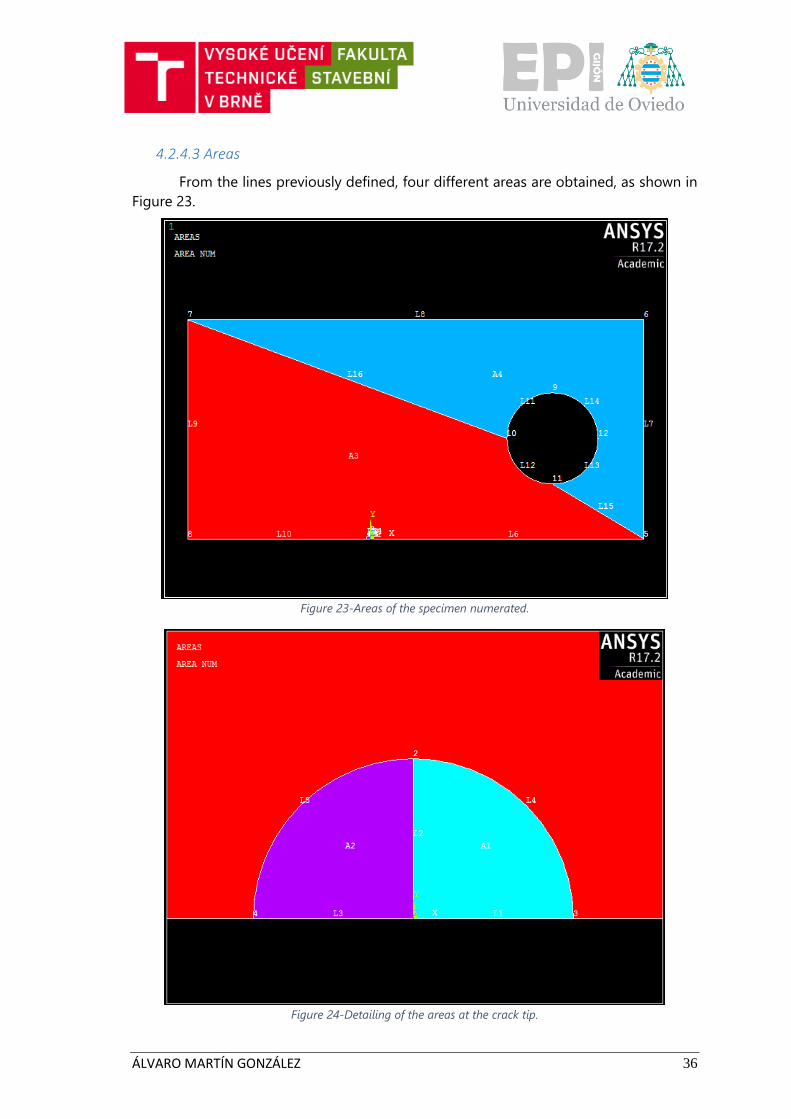
From the lines previously defined, four different areas are obtained, as shown in
Figure 23.
Figure 23-Areas of the specimen numerated.
Figure 24-Detailing of the areas at the crack tip.
ÁLVARO MARTÍN GONZÁLEZ 37
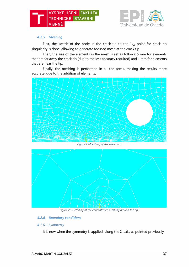
4.2.5 Meshing
First, the switch of the node in the crack-tip to the 14⁄ point for crack tip
singularity is done, allowing to generate focused mesh at the crack tip.
Then, the size of the elements in the mesh is set as follows: 5 mm for elements
that are far away the crack tip (due to the less accuracy required) and 1 mm for elements
that are near the tip.
Finally, the meshing is performed in all the areas, making the results more
accurate, due to the addition of elements.
Figure 25-Meshing of the specimen.
Figure 26-Detailing of the concentrated meshing around the tip.
4.2.6 Boundary conditions
4.2.6.1 Symmetry
It is now when the symmetry is applied, along the X-axis, as pointed previously.
ÁLVARO MARTÍN GONZÁLEZ 38
4.2.6.2 Supports
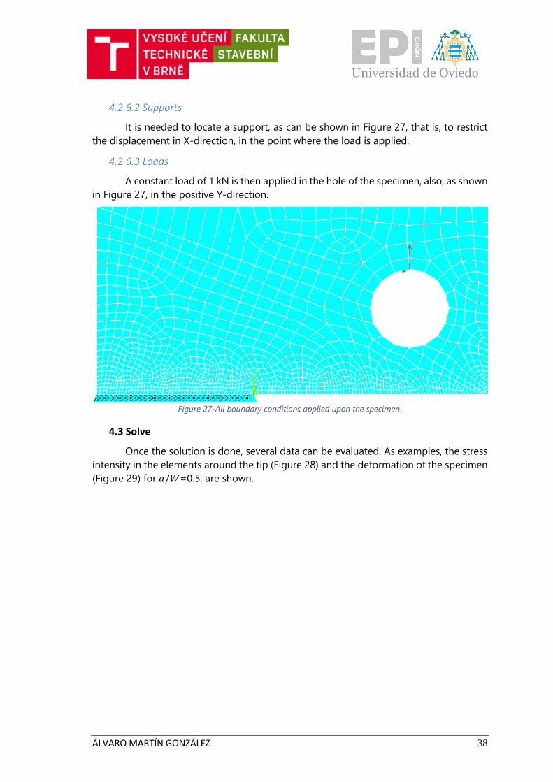
It is needed to locate a support, as can be shown in Figure 27, that is, to restrict
the displacement in X-direction, in the point where the load is applied.
4.2.6.3 Loads
A constant load of 1 kN is then applied in the hole of the specimen, also, as shown
in Figure 27, in the positive Y-direction.
Figure 27-All boundary conditions applied upon the specimen.
4.3 Solve
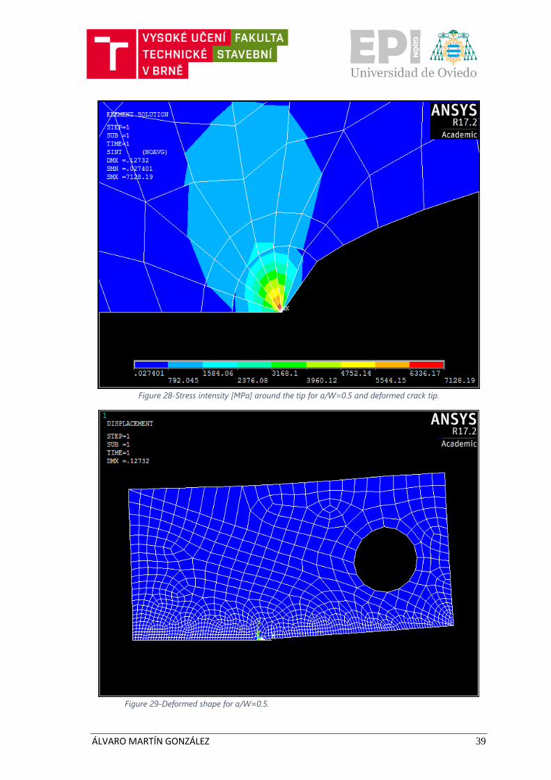
Once the solution is done, several data can be evaluated. As examples, the stress
intensity in the elements around the tip (Figure 28) and the deformation of the specimen
(Figure 29) for 𝑎/𝑊=0.5, are shown.
ÁLVARO MARTÍN GONZÁLEZ 39
Figure 28-Stress intensity [MPa] around the tip for a/W=0.5 and deformed crack tip.
Figure 29-Deformed shape for a/W=0.5.
ÁLVARO MARTÍN GONZÁLEZ 40
4.4 Post-processor
Once the model is created and solved, it is time to get both the SIF and the 𝑇-
stress.
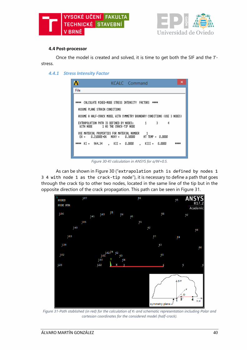
4.4.1 Stress Intensity Factor
Figure 30-KI calculation in ANSYS for a/W=0.5.
As can be shown in Figure 30 (“extrapolation path is defined by nodes 1
3 4 with node 1 as the crack-tip node”), it is necessary to define a path that goes
through the crack tip to other two nodes, located in the same line of the tip but in the
opposite direction of the crack propagation. This path can be seen in Figure 31.
Figure 31-Path stablished (in red) for the calculation of KI and schematic representation including Polar and
cartesian coordinates for the considered model (half-crack).
ÁLVARO MARTÍN GONZÁLEZ 41
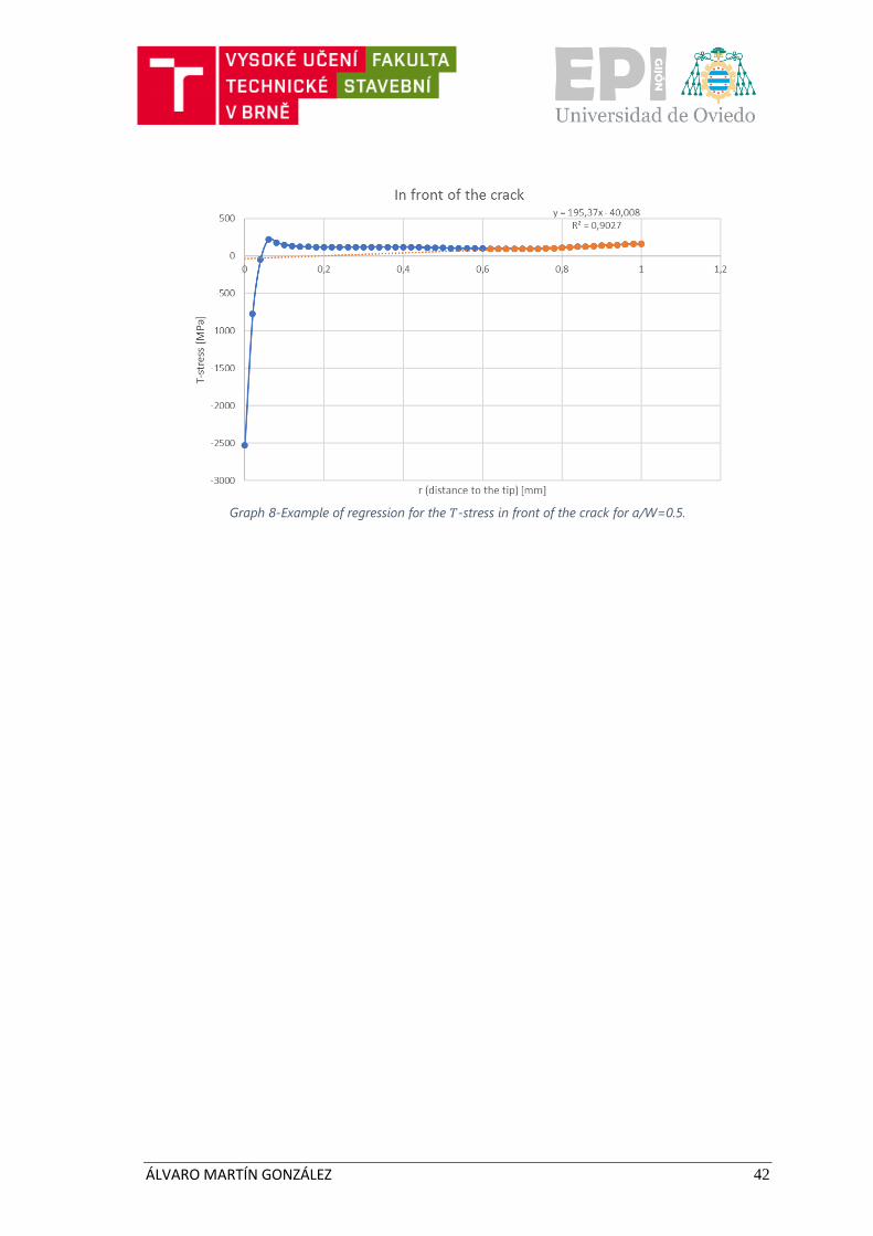
4.4.2 T-stress
Equation (3) was said to be the method used for the calculation of the 𝑇-stress,
so the aim is to get the stresses 𝜎𝑥𝑥, 𝜎𝑦𝑦 with ANSYS and then make the computation to
obtain the 𝑇-stress.
ANSYS interpolates the stress along the path, obtaining, then, average element
results across elements.
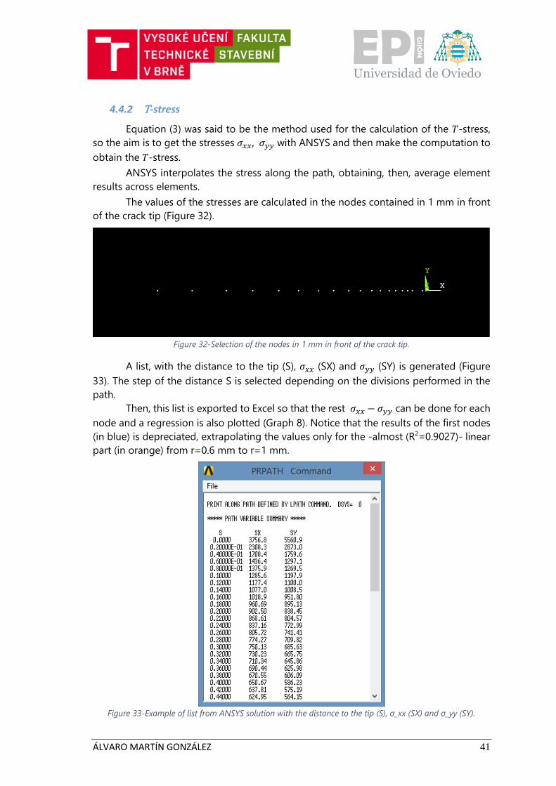
The values of the stresses are calculated in the nodes contained in 1 mm in front
of the crack tip (Figure 32).
Figure 32-Selection of the nodes in 1 mm in front of the crack tip.
A list, with the distance to the tip (S), 𝜎𝑥𝑥 (SX) and 𝜎𝑦𝑦 (SY) is generated (Figure
33). The step of the distance S is selected depending on the divisions performed in the
path.
Then, this list is exported to Excel so that the rest 𝜎𝑥𝑥 − 𝜎𝑦𝑦 can be done for each
node and a regression is also plotted (Graph 8). Notice that the results of the first nodes
(in blue) is depreciated, extrapolating the values only for the -almost (R2=0.9027)- linear
part (in orange) from r=0.6 mm to r=1 mm.
Figure 33-Example of list from ANSYS solution with the distance to the tip (S), σ_xx (SX) and σ_yy (SY).
ÁLVARO MARTÍN GONZÁLEZ 42
Graph 8-Example of regression for the 𝑇-stress in front of the crack for a/W=0.5.
ÁLVARO MARTÍN GONZÁLEZ 43
5. NUMERICAL RESULTS
5.1 Stress Intensity Factors
In the following, several graphs are prepared showing the values of the 𝐾𝐼
obtained through:
- ASTM literature calculations.
- Knésl and Bednar literature calculations.
- ANSYS calculations.
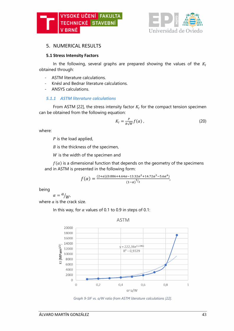
5.1.1 ASTM literature calculations
From ASTM [22], the stress intensity factor 𝐾𝐼 for the compact tension specimen
can be obtained from the following equation:
𝐾𝐼 =𝑃
𝐵√𝑊𝑓(𝛼) , (20)
where:
𝑃 is the load applied,
𝐵 is the thickness of the specimen,
𝑊 is the width of the specimen and
𝑓(𝛼) is a dimensional function that depends on the geometry of the specimens
and in ASTM is presented in the following form:
𝑓(𝛼) =(2+𝛼)(0.886+4.64𝛼−13.32𝛼2+14.72𝛼3−5.6𝛼4)
(1−𝛼)3
2⁄,
being
𝛼 = 𝑎𝑊⁄ ,
where 𝑎 is the crack size.
In this way, for 𝛼 values of 0.1 to 0.9 in steps of 0.1:
Graph 9-SIF vs. a/W ratio from ASTM literature calculations [22].
ÁLVARO MARTÍN GONZÁLEZ 44
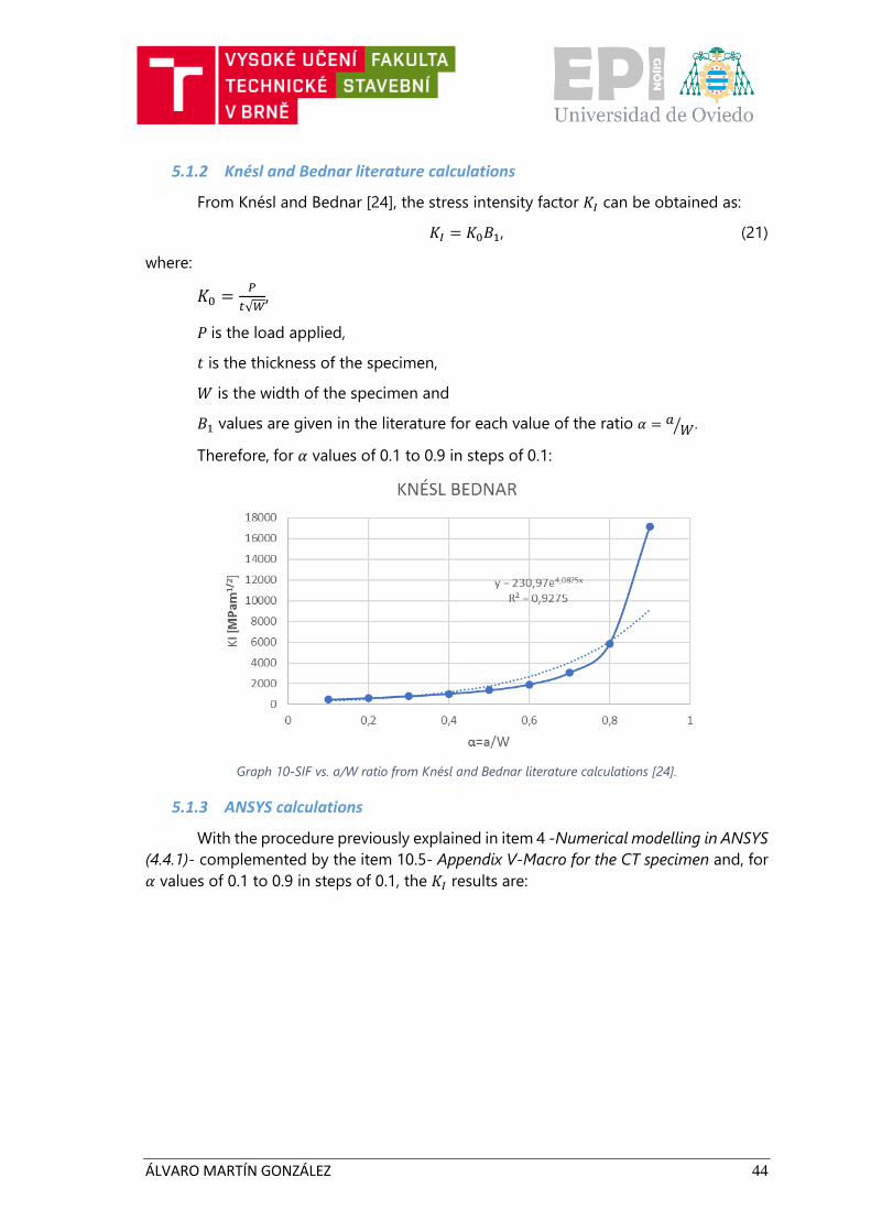
5.1.2 Knésl and Bednar literature calculations
From Knésl and Bednar [24], the stress intensity factor 𝐾𝐼 can be obtained as:
𝐾𝐼 = 𝐾0𝐵1, (21)
where:
𝐾0 =𝑃
𝑡√𝑊,
𝑃 is the load applied,
𝑡 is the thickness of the specimen,
𝑊 is the width of the specimen and
𝐵1 values are given in the literature for each value of the ratio 𝛼 = 𝑎𝑊⁄ .
Therefore, for 𝛼 values of 0.1 to 0.9 in steps of 0.1:
Graph 10-SIF vs. a/W ratio from Knésl and Bednar literature calculations [24].
5.1.3 ANSYS calculations
With the procedure previously explained in item 4 -Numerical modelling in ANSYS
(4.4.1)- complemented by the item 10.5- Appendix V-Macro for the CT specimen and, for 𝛼 values of 0.1 to 0.9 in steps of 0.1, the 𝐾𝐼 results are:
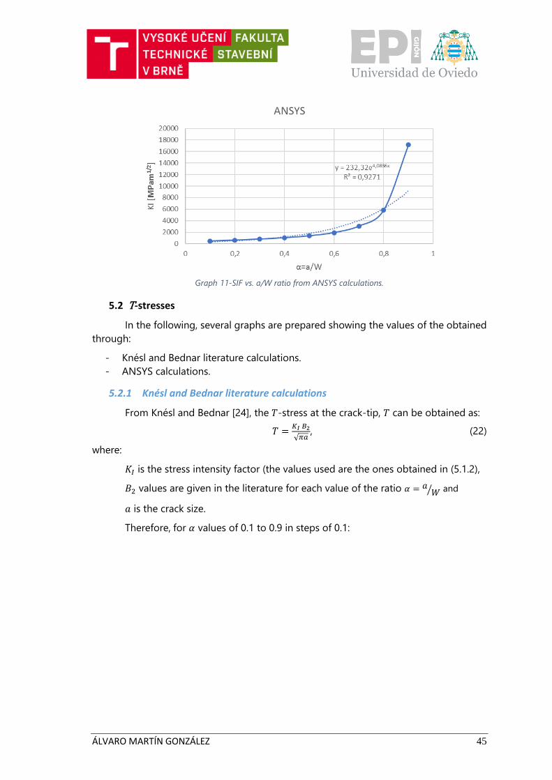
ÁLVARO MARTÍN GONZÁLEZ 45
Graph 11-SIF vs. a/W ratio from ANSYS calculations.
5.2 T-stresses
In the following, several graphs are prepared showing the values of the obtained
through:
- Knésl and Bednar literature calculations.
- ANSYS calculations.
5.2.1 Knésl and Bednar literature calculations
From Knésl and Bednar [24], the 𝑇-stress at the crack-tip, 𝑇 can be obtained as:
𝑇 =𝐾𝐼 𝐵2
√𝜋𝑎, (22)
where:
𝐾𝐼 is the stress intensity factor (the values used are the ones obtained in (5.1.2),
𝐵2 values are given in the literature for each value of the ratio 𝛼 = 𝑎𝑊⁄ and
𝑎 is the crack size.
Therefore, for 𝛼 values of 0.1 to 0.9 in steps of 0.1:
ÁLVARO MARTÍN GONZÁLEZ 46
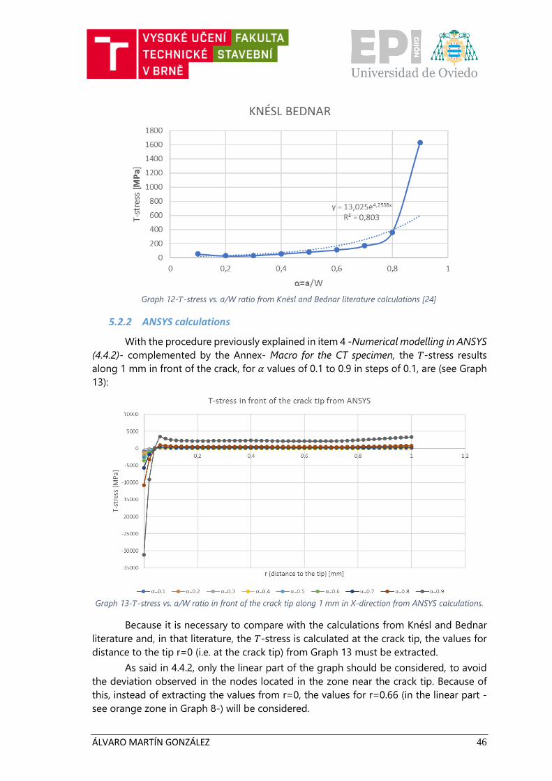
Graph 12-𝑇-stress vs. a/W ratio from Knésl and Bednar literature calculations [24]
5.2.2 ANSYS calculations
With the procedure previously explained in item 4 -Numerical modelling in ANSYS
(4.4.2)- complemented by the Annex- Macro for the CT specimen, the 𝑇-stress results
along 1 mm in front of the crack, for 𝛼 values of 0.1 to 0.9 in steps of 0.1, are (see Graph
13):
Graph 13-𝑇-stress vs. a/W ratio in front of the crack tip along 1 mm in X-direction from ANSYS calculations.
Because it is necessary to compare with the calculations from Knésl and Bednar
literature and, in that literature, the 𝑇-stress is calculated at the crack tip, the values for
distance to the tip r=0 (i.e. at the crack tip) from Graph 13 must be extracted.
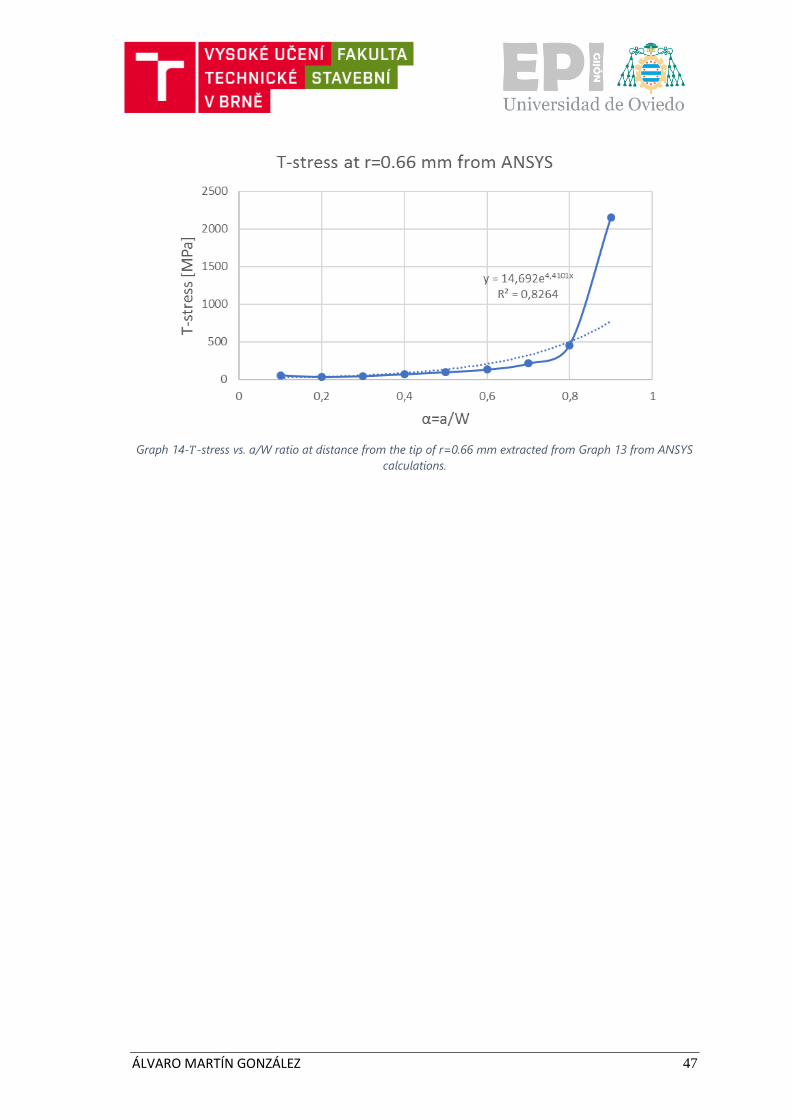
As said in 4.4.2, only the linear part of the graph should be considered, to avoid
the deviation observed in the nodes located in the zone near the crack tip. Because of
this, instead of extracting the values from r=0, the values for r=0.66 (in the linear part -
see orange zone in Graph 8-) will be considered.
ÁLVARO MARTÍN GONZÁLEZ 47
Graph 14-𝑇-stress vs. a/W ratio at distance from the tip of r=0.66 mm extracted from Graph 13 from ANSYS
calculations.
ÁLVARO MARTÍN GONZÁLEZ 48
6. VALUES OF S355 PUBLISHED IN LITERATURE
In this item, graphs from S355 steel experiments carried out in several articles are
going to be evaluated.
By means of a digitizer software, the graphs that are of interest for this thesis are
extracted from those articles and then converted to Excel graphs so that the values can
be evaluated.
Those experimental graphs are about:
-Stress-Number of Cycles curves.
-Crack propagation rate curves.
All the graphs are focused in the two different grades considered: S355 J0 and
S355 J2.
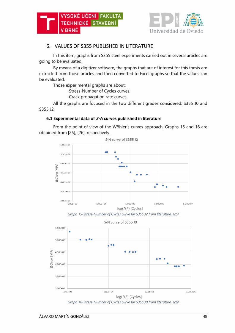
6.1 Experimental data of S-N curves published in literature
From the point of view of the Wöhler’s curves approach, Graphs 15 and 16 are
obtained from [25], [26], respectively.
Graph 15-Stress-Number of Cycles curve for S355 J2 from literature. [25]
Graph 16-Stress-Number of Cycles curve for S355 J0 from literature. [26]
ÁLVARO MARTÍN GONZÁLEZ 49
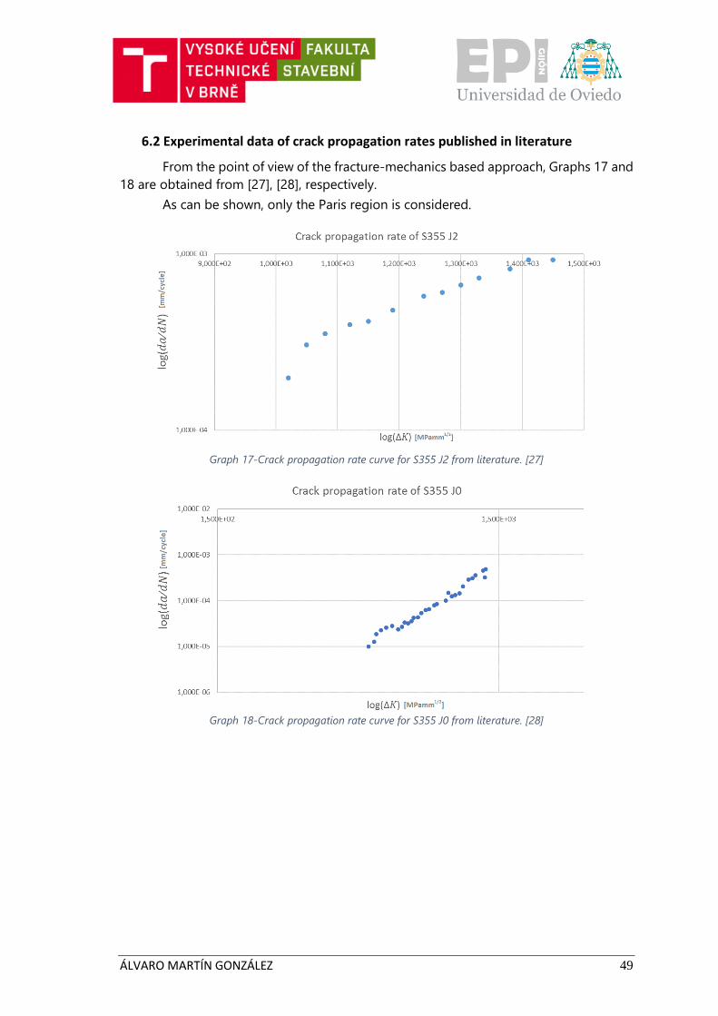
6.2 Experimental data of crack propagation rates published in literature
From the point of view of the fracture-mechanics based approach, Graphs 17 and
18 are obtained from [27], [28], respectively.
As can be shown, only the Paris region is considered.
Graph 17-Crack propagation rate curve for S355 J2 from literature. [27]
Graph 18-Crack propagation rate curve for S355 J0 from literature. [28]
ÁLVARO MARTÍN GONZÁLEZ 50
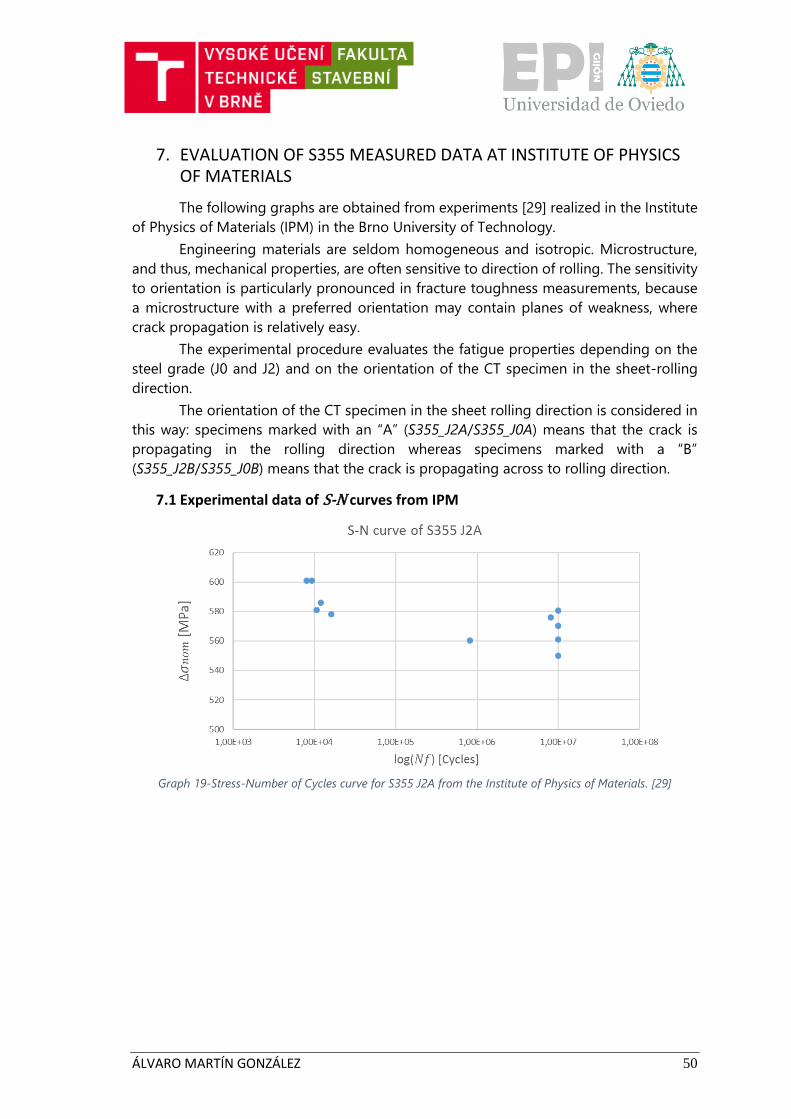
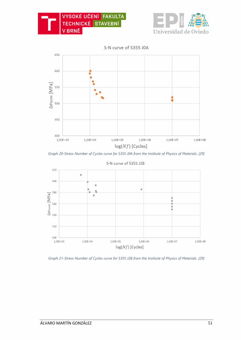
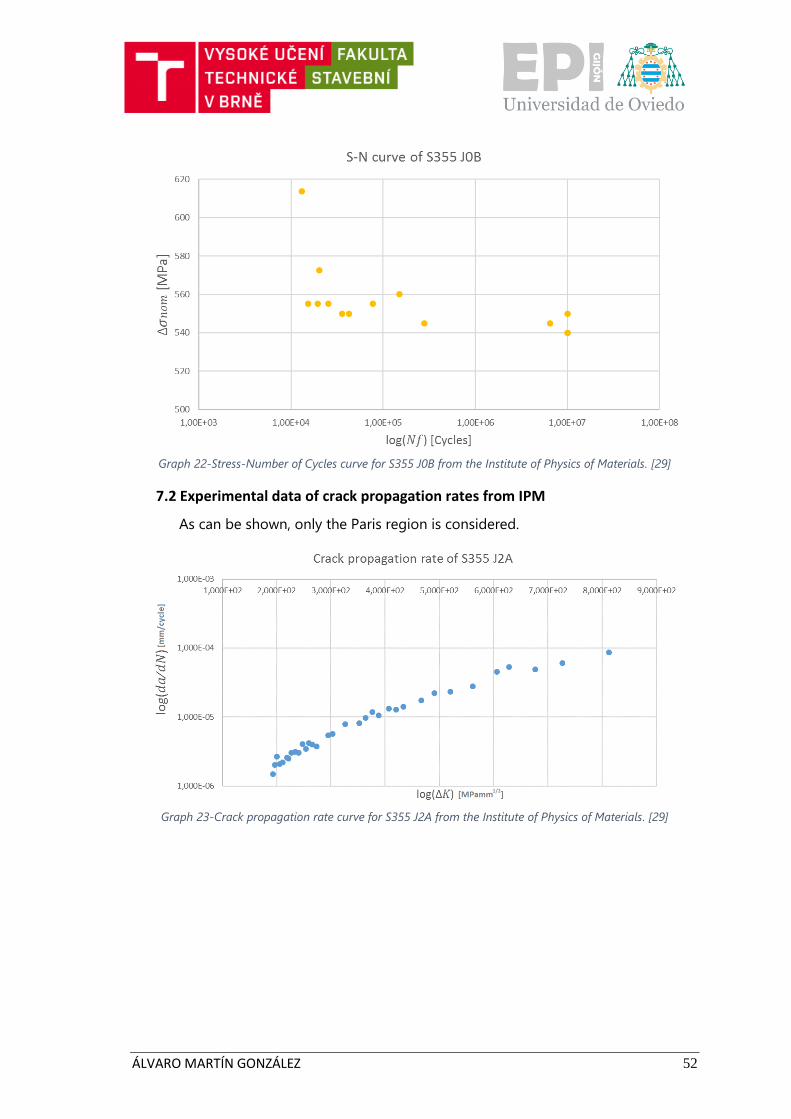
7. EVALUATION OF S355 MEASURED DATA AT INSTITUTE OF PHYSICS OF MATERIALS
The following graphs are obtained from experiments [29] realized in the Institute
of Physics of Materials (IPM) in the Brno University of Technology.
Engineering materials are seldom homogeneous and isotropic. Microstructure,
and thus, mechanical properties, are often sensitive to direction of rolling. The sensitivity
to orientation is particularly pronounced in fracture toughness measurements, because
a microstructure with a preferred orientation may contain planes of weakness, where
crack propagation is relatively easy.
The experimental procedure evaluates the fatigue properties depending on the
steel grade (J0 and J2) and on the orientation of the CT specimen in the sheet-rolling
direction.
The orientation of the CT specimen in the sheet rolling direction is considered in
this way: specimens marked with an “A” (S355_J2A/S355_J0A) means that the crack is
propagating in the rolling direction whereas specimens marked with a “B”
(S355_J2B/S355_J0B) means that the crack is propagating across to rolling direction.
7.1 Experimental data of S-N curves from IPM
Graph 19-Stress-Number of Cycles curve for S355 J2A from the Institute of Physics of Materials. [29]
ÁLVARO MARTÍN GONZÁLEZ 51
Graph 20-Stress-Number of Cycles curve for S355 J0A from the Institute of Physics of Materials. [29]
Graph 21-Stress-Number of Cycles curve for S355 J2B from the Institute of Physics of Materials. [29]
ÁLVARO MARTÍN GONZÁLEZ 52
Graph 22-Stress-Number of Cycles curve for S355 J0B from the Institute of Physics of Materials. [29]
7.2 Experimental data of crack propagation rates from IPM
As can be shown, only the Paris region is considered.
Graph 23-Crack propagation rate curve for S355 J2A from the Institute of Physics of Materials. [29]
ÁLVARO MARTÍN GONZÁLEZ 53
Graph 24-Crack propagation rate curve for S355 J0A from the Institute of Physics of Materials. [29]
Graph 25-Crack propagation rate curve for S355 J2B from the Institute of Physics of Materials. [29]
ÁLVARO MARTÍN GONZÁLEZ 54
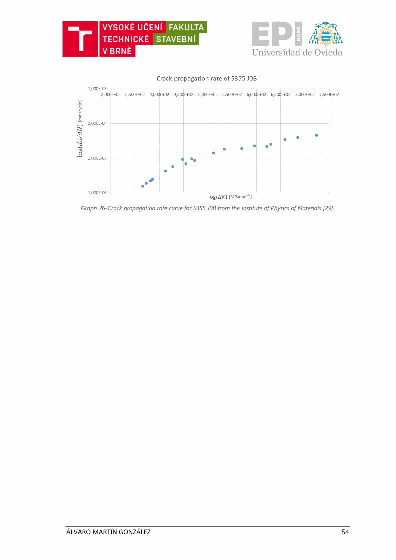
Graph 26-Crack propagation rate curve for S355 J0B from the Institute of Physics of Materials [29].
ÁLVARO MARTÍN GONZÁLEZ 55
8. COMPARISON AND DISCUSSION OF THE RESULTS
8.1 Comparison of curves from ANSYS and literature
8.1.1 Comparison of Stress Intensity Factor
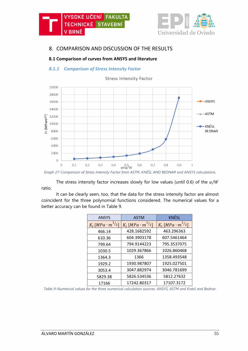
Graph 27-Comparison of Stress Intensity Factor from ASTM, KNÉSL AND BEDNAR and ANSYS calculations.
The stress intensity factor increases slowly for low values (until 0.6) of the 𝑎/𝑊
ratio.
It can be clearly seen, too, that the data for the stress intensity factor are almost
coincident for the three polynomial functions considered. The numerical values for a
better accuracy can be found in Table 9.
ANSYS ASTM KNÉSL
𝐾𝐼 [𝑀𝑃𝑎 ∙ 𝑚1
2⁄ ] 𝐾𝐼 [𝑀𝑃𝑎 ∙ 𝑚1
2⁄ ] 𝐾𝐼 [𝑀𝑃𝑎 ∙ 𝑚1
2⁄ ]
466.14 428.1682592 463.296363
610.36 604.3903178 607.5461464
799.64 794.9144223 795.3537075
1030.5 1029.367866 1026.860468
1364.3 1366 1358.493548
1929.2 1930.987807 1925.027501
3053.4 3047.882974 3046.781699
5829.38 5826.534536 5812.27632
17166 17242.80317 17107.3172
Table 9-Numerical values for the three numerical calculation sources: ANSYS, ASTM and Knésl and Bednar.
ÁLVARO MARTÍN GONZÁLEZ 56
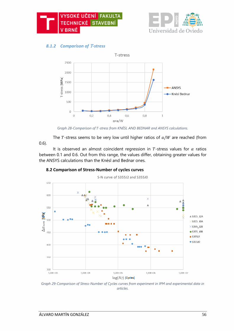
8.1.2 Comparison of T-stress
Graph 28-Comparison of 𝑇-stress from KNÉSL AND BEDNAR and ANSYS calculations.
The 𝑇-stress seems to be very low until higher ratios of 𝑎/𝑊 are reached (from
0.6).
It is observed an almost coincident regression in 𝑇-stress values for 𝛼 ratios
between 0.1 and 0.6. Out from this range, the values differ, obtaining greater values for
the ANSYS calculations than the Knésl and Bednar ones.
8.2 Comparison of Stress-Number of cycles curves
Graph 29-Comparison of Stress-Number of Cycles curves from experiment in IPM and experimental data in
articles.
ÁLVARO MARTÍN GONZÁLEZ 57
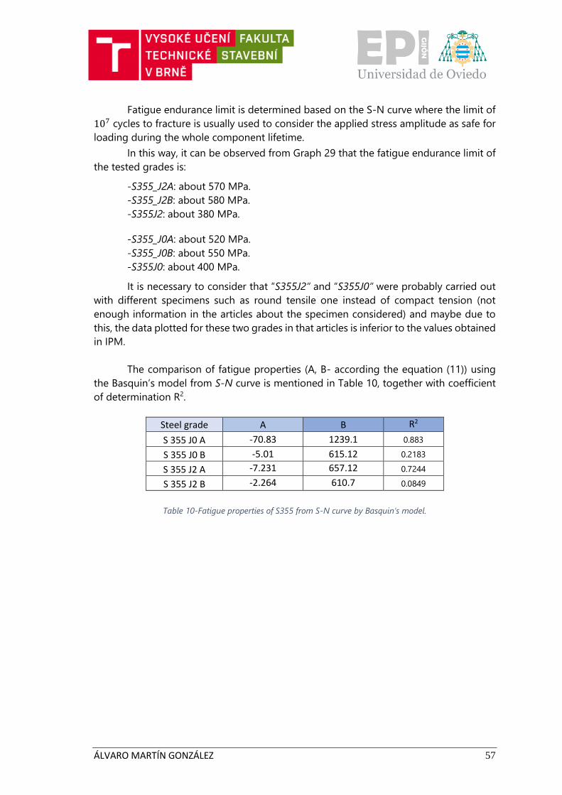
Fatigue endurance limit is determined based on the S-N curve where the limit of
107 cycles to fracture is usually used to consider the applied stress amplitude as safe for
loading during the whole component lifetime.
In this way, it can be observed from Graph 29 that the fatigue endurance limit of
the tested grades is:
-S355_J2A: about 570 MPa.
-S355_J2B: about 580 MPa.
-S355J2: about 380 MPa.
-S355_J0A: about 520 MPa.
-S355_J0B: about 550 MPa.
-S355J0: about 400 MPa.
It is necessary to consider that “S355J2” and “S355J0” were probably carried out
with different specimens such as round tensile one instead of compact tension (not
enough information in the articles about the specimen considered) and maybe due to
this, the data plotted for these two grades in that articles is inferior to the values obtained
in IPM.
The comparison of fatigue properties (A, B- according the equation (11)) using
the Basquin’s model from S-N curve is mentioned in Table 10, together with coefficient
of determination R2.
Steel grade A B R2
S 355 J0 A -70.83 1239.1 0.883
S 355 J0 B -5.01 615.12 0.2183
S 355 J2 A -7.231 657.12 0.7244
S 355 J2 B -2.264 610.7 0.0849
Table 10-Fatigue properties of S355 from S-N curve by Basquin’s model.
ÁLVARO MARTÍN GONZÁLEZ 58
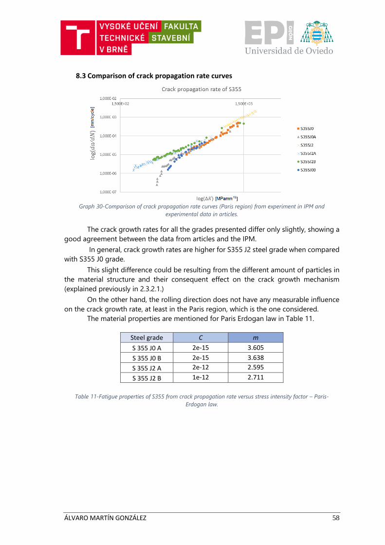
8.3 Comparison of crack propagation rate curves
Graph 30-Comparison of crack propagation rate curves (Paris region) from experiment in IPM and
experimental data in articles.
The crack growth rates for all the grades presented differ only slightly, showing a
good agreement between the data from articles and the IPM.
In general, crack growth rates are higher for S355 J2 steel grade when compared
with S355 J0 grade.
This slight difference could be resulting from the different amount of particles in
the material structure and their consequent effect on the crack growth mechanism
(explained previously in 2.3.2.1.)
On the other hand, the rolling direction does not have any measurable influence
on the crack growth rate, at least in the Paris region, which is the one considered.
The material properties are mentioned for Paris Erdogan law in Table 11.
Steel grade C m
S 355 J0 A 2e-15 3.605
S 355 J0 B 2e-15 3.638
S 355 J2 A 2e-12 2.595
S 355 J2 B 1e-12 2.711
Table 11-Fatigue properties of S355 from crack propagation rate versus stress intensity factor – Paris-
Erdogan law.
ÁLVARO MARTÍN GONZÁLEZ 59
9. CONCLUSIONS
In this thesis, two different parameters for the definition of the crack-tip
conditions: Stress Intensity Factor and 𝑇-stress, and two different approaches to fatigue
analysis (in two different S355 grades): statistics (Wöhler‘s curve) and Fracture Mechanics
(Crack Propagation Rate curve), were evaluated and compared with experimental data
and data from literature.
The following conclusions can be drawn:
• The three formulas (polynomial functions) for the calculation of the SIF (ANSYS,
ASTM, Knésl and Bednar) show a very good agreement between them.
• ANSYS’ and Knésl and Bednar’s obtained values seem to be a good approach for the
calculation of the 𝑇-stress at the crack tip since they show a good agreement
between them.
• In general, S355 J2 grade exhibit a greater fatigue-endurance limit.
• There is none appreciable difference between the fatigue-endurance limits of
specimens with the same grade but different rolling direction.
• The S355 J2 steel grade exhibits higher crack growth rates when compared with the
S355 J0 steel grade.
• The crack growth rate seems to be independent of the rolling direction and, thus,
resulting structure.
• Both S-N and 𝑑𝑎𝑑𝑁⁄ -∆𝐾 curves seem to be influenced only by the different chemical
composition of the considered steel grades.
ÁLVARO MARTÍN GONZÁLEZ 60
10. APPENDIX
10.1 APPENDIX I - Nomenclature
𝑎 Crack size
𝐹𝐸 Finite Elements
𝐾 or 𝑆𝐼𝐹 Stress Intensity Factor
𝐾𝐼 Stress Intensity Factor (Mode I)
𝑃 Load applied
𝑟 Distance from the crack tip (Cartesian coordinate)
𝐵 or 𝑡 Thickness of the specimen
𝜃 Angular coordinate
𝜎𝑌𝑆 Yield Strength
𝜎 or 𝑆 Stress
𝐿𝐸𝐹𝑀 Linear Elastic Fracture Mechanics
𝐸𝑃𝐹𝑀 Elastic Plastic Fracture Mechanics
𝐶𝑇𝑂𝐷 or 𝛿 Crack Tip Opening Displacement
𝐶𝑇 Compact Tension
𝜈 Poisson’s ratio
𝐸 Young’s modulus
𝑊 Width of specimen
𝑇 𝑇-stress
𝜌 Density
𝑈𝑇𝑆 Ultimate Tensile Strength
𝐾𝐼𝑐 Critical value of the Stress Intensity Factor (Fracture toughness)
∆𝐾 Stress Intensity Factor range
𝐿𝐶𝐹 Low Cycle Fatigue
𝐻𝐶𝐹 High Cycle Fatigue
𝑁 Number of cycles
ÁLVARO MARTÍN GONZÁLEZ 61
10.2 APPENDIX II - List of figures
Figure 1-Definition of the coordinate system with origin in crack tip: Polar and
Cartesian. [9] ................................................................................................................................................... 8
Figure 2-The three modes of loading that a crack can experience. [9] .................................... 9
Figure 3-Definition of Polar coordinates with 𝜃 = 0 [9]............................................................... 10
Figure 4-Alternative definitions of CTOD: (a) displacement at the original crack tip and
(b) displacement at the intersection of a 90º vertex with the crack flanks. [9] ................... 11
Figure 5-Small-scale yielding condition. [9] ..................................................................................... 13
Figure 6-Typical fatigue fracture appearance. ................................................................................. 15
Figure 7-Stages of the lifecycle of a fatigue crack. [11] ............................................................... 15
Figure 8-Crack nucleation from inclusions. [2] ................................................................................ 16
Figure 9-Microstructurally short crack. [11] ...................................................................................... 17
Figure 10-Mechanically short crack. [11] ........................................................................................... 18
Figure 11-Long crack. [11] ....................................................................................................................... 18
Figure 12-Typical CT specimen [21]. .................................................................................................... 24
Figure 13-CT dimensions. [22] ............................................................................................................... 25
Figure 14-Apparatus for testing CT specimens. [9] ....................................................................... 26
Figure 15-List of some of the element types available in ANSYS. ........................................... 31
Figure 16-PLANE82, 2-D, 8-Node, Structural Solid. [23] .............................................................. 32
Figure 17-Linear isotropic properties for steel. Young’s modulus (EX) [MPa] and
Poisson’s number (NUXY) [-]. ................................................................................................................. 33
Figure 18-Plane of symmetry (in red) considered. ......................................................................... 33
Figure 19-KP of the specimen numerated. ....................................................................................... 34
Figure 20-Detailing of the KP at the crack tip.................................................................................. 34
Figure 21-Lines of the specimen numerated. .................................................................................. 35
Figure 22-Detailing of the lines at the crack tip. ............................................................................. 35
Figure 23-Areas of the specimen numerated. ................................................................................. 36
Figure 24-Detailing of the areas at the crack tip. ........................................................................... 36
Figure 25-Meshing of the specimen. .................................................................................................. 37
Figure 26-Detailing of the concentrated meshing around the tip. .......................................... 37
Figure 27-All boundary conditions applied upon the specimen. ............................................. 38
Figure 28-Stress intensity [MPa] around the tip for a/W=0.5 and deformed crack tip. .. 39
Figure 29-Deformed shape for a/W=0.5. .......................................................................................... 39
Figure 30-KI calculation in ANSYS for a/W=0.5. ............................................................................. 40
Figure 31-Path stablished (in red) for the calculation of KI and schematic representation
including Polar and cartesian coordinates for the considered model (half-crack). ........... 40
Figure 32-Selection of the nodes in 1 mm in front of the crack tip. ....................................... 41
Figure 33-Example of list from ANSYS solution with the distance to the tip (S), σ_xx (SX)
and σ_yy (SY). ............................................................................................................................................... 41
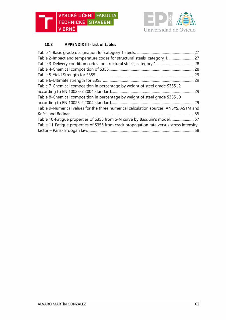
ÁLVARO MARTÍN GONZÁLEZ 62
10.3 APPENDIX III - List of tables
Table 1-Basic grade designation for category 1 steels. ............................................................... 27
Table 2-Impact and temperature codes for structural steels, category 1. ............................ 27
Table 3-Delivery condition codes for structural steels, category 1. ......................................... 28
Table 4-Chemical composition of S355. ............................................................................................ 28
Table 5-Yield Strength for S355. ........................................................................................................... 29
Table 6-Ultimate strength for S355. .................................................................................................... 29
Table 7-Chemical composition in percentage by weight of steel grade S355 J2
according to EN 10025-2:2004 standard. .......................................................................................... 29
Table 8-Chemical composition in percentage by weight of steel grade S355 J0
according to EN 10025-2:2004 standard. .......................................................................................... 29
Table 9-Numerical values for the three numerical calculation sources: ANSYS, ASTM and
Knésl and Bednar. ....................................................................................................................................... 55
Table 10-Fatigue properties of S355 from S-N curve by Basquin’s model. ......................... 57
Table 11-Fatigue properties of S355 from crack propagation rate versus stress intensity
factor – Paris- Erdogan law. .................................................................................................................... 58
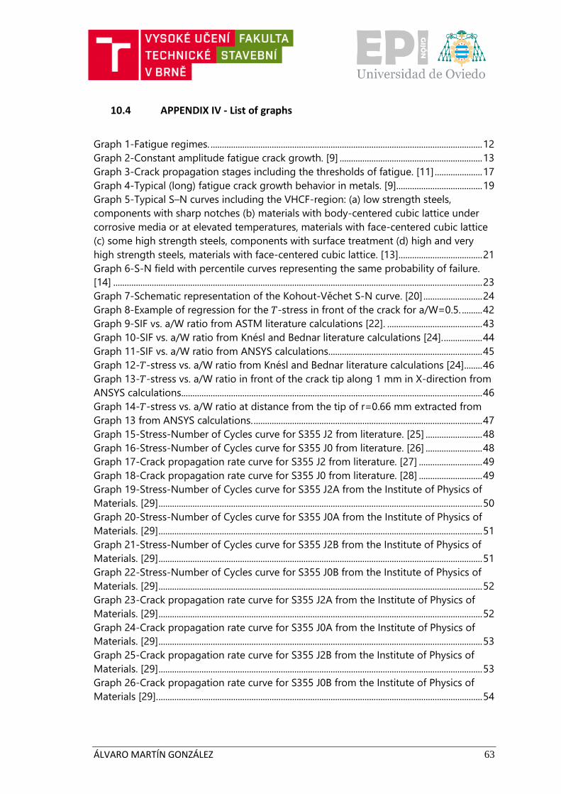
ÁLVARO MARTÍN GONZÁLEZ 63
10.4 APPENDIX IV - List of graphs
Graph 1-Fatigue regimes. ........................................................................................................................ 12
Graph 2-Constant amplitude fatigue crack growth. [9] ............................................................... 13
Graph 3-Crack propagation stages including the thresholds of fatigue. [11] ..................... 17
Graph 4-Typical (long) fatigue crack growth behavior in metals. [9] ...................................... 19
Graph 5-Typical S–N curves including the VHCF-region: (a) low strength steels,
components with sharp notches (b) materials with body-centered cubic lattice under
corrosive media or at elevated temperatures, materials with face-centered cubic lattice
(c) some high strength steels, components with surface treatment (d) high and very
high strength steels, materials with face-centered cubic lattice. [13] ..................................... 21
Graph 6-S-N field with percentile curves representing the same probability of failure.
[14] ................................................................................................................................................................... 23
Graph 7-Schematic representation of the Kohout-Věchet S-N curve. [20] .......................... 24
Graph 8-Example of regression for the 𝑇-stress in front of the crack for a/W=0.5. ......... 42
Graph 9-SIF vs. a/W ratio from ASTM literature calculations [22]. .......................................... 43
Graph 10-SIF vs. a/W ratio from Knésl and Bednar literature calculations [24]. ................. 44
Graph 11-SIF vs. a/W ratio from ANSYS calculations.................................................................... 45
Graph 12-𝑇-stress vs. a/W ratio from Knésl and Bednar literature calculations [24] ........ 46
Graph 13-𝑇-stress vs. a/W ratio in front of the crack tip along 1 mm in X-direction from
ANSYS calculations..................................................................................................................................... 46
Graph 14-𝑇-stress vs. a/W ratio at distance from the tip of r=0.66 mm extracted from
Graph 13 from ANSYS calculations. ..................................................................................................... 47
Graph 15-Stress-Number of Cycles curve for S355 J2 from literature. [25] ......................... 48
Graph 16-Stress-Number of Cycles curve for S355 J0 from literature. [26] ......................... 48
Graph 17-Crack propagation rate curve for S355 J2 from literature. [27] ............................ 49
Graph 18-Crack propagation rate curve for S355 J0 from literature. [28] ............................ 49
Graph 19-Stress-Number of Cycles curve for S355 J2A from the Institute of Physics of
Materials. [29] ............................................................................................................................................... 50
Graph 20-Stress-Number of Cycles curve for S355 J0A from the Institute of Physics of
Materials. [29] ............................................................................................................................................... 51
Graph 21-Stress-Number of Cycles curve for S355 J2B from the Institute of Physics of
Materials. [29] ............................................................................................................................................... 51
Graph 22-Stress-Number of Cycles curve for S355 J0B from the Institute of Physics of
Materials. [29] ............................................................................................................................................... 52
Graph 23-Crack propagation rate curve for S355 J2A from the Institute of Physics of
Materials. [29] ............................................................................................................................................... 52
Graph 24-Crack propagation rate curve for S355 J0A from the Institute of Physics of
Materials. [29] ............................................................................................................................................... 53
Graph 25-Crack propagation rate curve for S355 J2B from the Institute of Physics of
Materials. [29] ............................................................................................................................................... 53
Graph 26-Crack propagation rate curve for S355 J0B from the Institute of Physics of
Materials [29]. ............................................................................................................................................... 54

ÁLVARO MARTÍN GONZÁLEZ 64
Graph 27-Comparison of Stress Intensity Factor from ASTM, KNÉSL AND BEDNAR and
ANSYS calculations..................................................................................................................................... 55
Graph 28-Comparison of 𝑇-stress from KNÉSL AND BEDNAR and ANSYS calculations. 56
Graph 29-Comparison of Stress-Number of Cycles curves from experiment in IPM and
experimental data in articles. ................................................................................................................. 56
Graph 30-Comparison of crack propagation rate curves (Paris region) from experiment
in IPM and experimental data in articles. .......................................................................................... 58
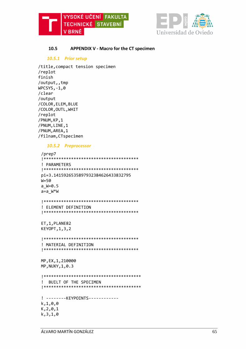
ÁLVARO MARTÍN GONZÁLEZ 65
10.5 APPENDIX V - Macro for the CT specimen
10.5.1 Prior setup
/title,compact tension specimen /replot finish /output,,tmp WPCSYS,-1,0 /clear /output /COLOR,ELEM,BLUE /COLOR,OUTL,WHIT /replot /PNUM,KP,1 /PNUM,LINE,1 /PNUM,AREA,1 /filnam,CTspecimen
10.5.2 Preprocessor
/prep7 !************************************** ! PARAMETERS !************************************** pi=3.1415926535897932384626433832795 W=50 a_W=0.5 a=a_W*W !************************************** ! ELEMENT DEFINITION !************************************** ET,1,PLANE82 KEYOPT,1,3,2 !************************************** ! MATERIAL DEFINITION !************************************** MP,EX,1,210000 MP,NUXY,1,0.3 !*************************************** ! BUILT OF THE SPECIMEN !*************************************** ! --------KEYPOINTS------------ k,1,0,0 K,2,0,1 k,3,1,0
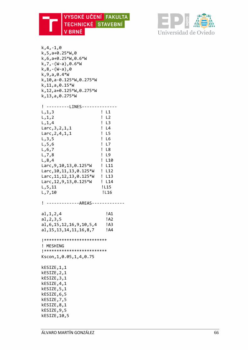
ÁLVARO MARTÍN GONZÁLEZ 66
k,4,-1,0 k,5,a+0.25*W,0 k,6,a+0.25*W,0.6*W k,7,-(W-a),0.6*W k,8,-(W-a),0 k,9,a,0.4*W k,10,a-0.125*W,0.275*W k,11,a,0.15*W k,12,a+0.125*W,0.275*W k,13,a,0.275*W ! ---------LINES-------------- L,1,3 ! L1 L,1,2 ! L2 L,1,4 ! L3 Larc,3,2,1,1 ! L4 Larc,2,4,1,1 ! L5 L,3,5 ! L6 L,5,6 ! L7 L,6,7 ! L8 L,7,8 ! L9 L,8,4 ! L10 Larc,9,10,13,0.125*W ! L11 Larc,10,11,13,0.125*W ! L12 Larc,11,12,13,0.125*W ! L13 Larc,12,9,13,0.125*W ! L14 L,5,11 !L15 L,7,10 !L16 ! -------------AREAS------------- al,1,2,4 !A1 al,2,3,5 !A2 al,6,15,12,16,9,10,5,4 !A3 al,15,13,14,11,16,8,7 !A4 !************************* ! MESHING !************************* Kscon,1,0.05,1,4,0.75 kESIZE,1,1 kESIZE,2,1 kESIZE,3,1 kESIZE,4,1 kESIZE,5,1 kESIZE,6,5 kESIZE,7,5 kESIZE,8,1 kESIZE,9,5 kESIZE,10,5
ÁLVARO MARTÍN GONZÁLEZ 67
kESIZE,11,5 kESIZE,12,5 kESIZE,13,5 !Material TYPE,1 MAT,1 AMESH,1 AMESH,2 AMESH,3 AMESH,4 FINISH
10.5.3 Solve
!*********************************************************** ! BOUNDARY CONDITIONS !*********************************************************** !---------SYMMETRY------------ /solu NSEL,S,LOC,X,0,-(W-a) NSEL,R,LOC,Y,0,0 DSYM,SYMM,y, , allsel, all !----------SUPPORTS------------ NSEL,S,LOC,X,a,a NSEL,R,Loc,y,0.4*W,0.4*W D,all, ,0, , , ,Ux, , , , , allsel,all eplot !------------LOADS------------- FK,9,FY,1000 allsel,all eplot solve FINISH
10.5.4 Postprocessing
10.5.4.1 Calculation of SIF
/POST1
ÁLVARO MARTÍN GONZÁLEZ 68
eplot
LPATH,1,3,4
KCALC,0,1,0,0
10.5.4.2 Calculation of 𝑇-stress (along 1 mm in front of the crack)
*NOTE: the procedure was made by means of the GUI.
NSEL,S,LOC,X,-1,0
NSEL,R,LOC,Y,0,0
nplot
/POST1
FLST,2,2,1
FITEM,2,1
FITEM,2,118
PATH,Tstress1,2,50,50,
PPATH,P51X,1
PATH,STAT
/REPLOT,RESIZE
AVPRIN,0, ,
PDEF, ,S,X,AVG
/PBC,PATH, ,0
AVPRIN,0, ,
PDEF, ,S,Y,AVG
/PBC,PATH, ,0
PRPATH,SX,SY
ÁLVARO MARTÍN GONZÁLEZ 69
11. REFERENCES
[1] P.-a. H. Wirsching, Statistical summaries of fatigue data for design purposes,
NASA contractor report.
[2] J. Belzunce, Tecnología de materiales-Comportamiento en servicio de materiales,
University of Oviedo, 2012.
[3] W. A. J. Albert, Uber Treibseile am Harz, Archiv fur Mineralogie Geognosie
Bergbau und Huttenkunde, 1838.
[4] A. A. Griffith, The fenomena of rupture and flow in solids, 1921.
[5] E. Paris P. C., A critical anaysis of crack propagation laws, J. Basic Eng., 1963.
[6] W. Weibull, A Statistical Theory Of The Strength Of Materials, Stockholm, 1939.
[7] ASTM, Symposium on Fatigue With Emphasis on Statistical Approach, June 1952.
[8] ASTM, Symposium on Statistical Aspects of Fatigue, June 1951.
[9] P. T.L Anderson, Fracture Mechanics: fundamentals and applications, Boca Raton:
Taylor & Francis group, Third edition-2005.
[10] A. F. Canteli, A statistical model for crack growth based on tension and
compression Wöhler fields, -: Elsevier Ltd., 2008.
[11] e. a. Zerbst U, Fatigue strength and fracture mechanics – A general perspective.,
Berlin: Elsevier Ltd.- Engng Fract Mech., 2017.
[12] ASTM, ASTM Standard Test Method For Measurement of Fatigue Crack Growth
Rates, West Conshohocken, PA, 1999.
[13] A. F. Canteli, Comparison of different statistical models for description of fatigue
including very high cycle fatigue, 2016.
[14] E. Castillo, Using statistical compatibility to derive advanced probabilistic fatigue
models, 2010.
[15] E. F. C. A. Castillo, A general regression model for lifetime evaluation and
prediction., Int. Journal of fracture, 2001.
[16] E. L.-A. M. R. A. F.-C. A. E. V. K. R. Castillo, Length effect on the fatigue strength of
prestressing wires and strands. Analysis of the independence model., Int. J. of
Fatigue.
[17] E. F.-C. A. H. A. Castillo, On fitting a fatigue model to data., Int. J. of Fatigue, 1999.
[18] O. M. D. R. T. K. Chaminda SS, Different approaches for remaining fatigue life
estimation of critical members in railway bridges., 2007.
[19] J. K. R., A new approach for estimating fatigue life in offshore steel structures,
Stavanger, Norway: Faculty of Science and Technology: MSc. Thesis..
[20] A. C. J.A.F.O. Correia, A generalization of the fatigue Kohout-Vechet model for
several fatigue damage parameters, Elsevier, 2017.
[21] en.wikipedia.org.
ÁLVARO MARTÍN GONZÁLEZ 70
[22] ASTM, Standard test method for measurement of fracture toughness.
[23] ANSYS, “Mechanical APDL Element Reference”.
[24] B. S. S. Knésl, Values of the first four coefficients of the William's expansion for
basic types of mechanical fracture testing bodies (in Czech language), Brno:
Institute of Physics of Materials, Academy of sciences.
[25] P. S. Tomas Tomaszewski, Analytical models of the S-N curves based on the
hardness of the material, Funchal, Madeira, Portugal: 2nd International Conference
on Structural Integrity, ICSI 2017. Elsevier, 4-7 September 2017.
[26] G. SZALA, Stress sensivity coefficient of a material in the range of high-cycle
fatigue, University of Technology and Life Sciences, Bydgoszcz, Poland.
[27] O. Adepipe, Review of corrosion fatigue in offshore structures: Present status and
challenges in offshore wind sector, Renewwable and Suistainable Energy Reviews.,
2016.
[28] A. M. P. De Jesus, A comparison of the fatigue behavior between S355 and S690
steel grades, Journal of construction Steel Research, 2012.
[29] S. SEITL, Comparison of the Fatigue Crack Propagation Rates in S355 J0 and S355
J2 Steel Grades, Brno, Czech Republic: Key Engineering Materials in Press.
[30] ANSYS, Mechanical APDL command reference.
[31] ANSYS, Mechanical APDL theory reference.
[32] A. J. Contreras, “Comportamiento a fatiga de los materiales,” Engineering &
Materials, 2014. [Online]. Available:
https://materialsbreakthroughs.wordpress.com.
[33] E. Castillo, A new probabilistic model for crack propagation under fatigue loads
and its connection with Wöhler fields., -: Elsevier Ltd., 2009.
[34] E. Castillo, Comparative analysis of two models for evaluating fatigue data., 2009.
[35] E. 10025-2:2004, European standard for hot-rolled structural steel. Part 2-
Technical delivery conditions for non-alloy structural steels.
[36] E. 1. E. Standard, S355 Standard Structural Steel Plate, 2004.
ÁLVARO MARTÍN GONZÁLEZ 71
12. CURRICULUM VITAE
PERSONAL INFORMATION
• Name: Álvaro Martín González
• Birth: May 16, 1996 (22 years)
• Place of birth: Oviedo (Asturias), Spain
• ID: 71738151-R
• Address: Manuel Fernández Avello St, no. 6, 5-A,
33011, Oviedo, Spain.
• Phone numbers: +34 616759981, +34 985114615
• E-mail: [email protected]
STUDIES
• Mechanical Engineering bachelor taught in English (4 years) with a mention
in construction at University of Oviedo - Gijón Polytechnic School of
Engineering (2014-2018)
• Erasmus+ mobility (1 year) in Brno University of Technology (Faculty of Civil
Engineering), Brno, Czech Republic (2017-2018). Taking the courses of the
last academic year including the Final Bachelor Thesis.
• Technological baccalaureate (2 years) at Colegio Loyola P.P. Escolapios,
Oviedo (Asturias), Spain (2012-2014).
• Secondary Education (4 years) at Colegio Loyola P.P. Escolapios, Oviedo
(Asturias), Spain (2008-2012).
LANGUAGES
• Spanish: native.
• English: Trinity College London – B2.

ÁLVARO MARTÍN GONZÁLEZ 72
COMPUTER SKILLS
• Medium-to-high level: AutoCad, ANSYS, LISAFEA, Autodesk Inventor, CESPLA.
• Medium-to-high level: Microsoft Office (Word, Excel, PowerPoint, Access).
• Basic Formation: EES, Matlab, Wxmaxima.
APTITUDES AND PERSONAL SKILLS
• Work-in-team capability.
• Leadership capability.
• Effort, perseverance and dedication.
• Adaptive capability.
• Good presence.
ADDITIONAL INFORMATION
• European Driving License – B (Spain).
• Own car, willingness to travel.