Embed Size (px)
Citation preview
http://tam.northwestern.edu/summerinstitute/Home.htm http://tam.northwestern.edu/wkl/liu.html
Bridging-Scale Methods and A Brief Introduction to Finite Element Methods
Wing Kam Liu
Northwestern University
Department of Mechanical Engineering
http://tam.northwestern.edu/summerinstitute/Home.htm http://tam.northwestern.edu/wkl/liu.html
Multiple Scale References
• F.F. Abraham, J. Broughton, N. Bernstein and E. Kaxiras, Europhysics Letters1998; 44:783-787
• E. Tadmor, M. Ortiz and R. Phillips, Philosophical Magazine A 1996; 73:1529-1563
• L. Shilkrot, W.A. Curtin and R.E. Miller, Journal of the Mechanics and Physics of Solids 2002; 50:2085-2106
• G.J. Wagner and W.K. Liu, Journal of Computational Physics 2003; 190:249-274• W.K. Liu, E.G. Karpov, S. Zhang and H.S. Park. “An Introduction to
Computational Nano Mechanics and Materials.” Computer Methods in Applied Mechanics and Engineering 2004; 193: 1529-1578.
• H.S. Park and W.K. Liu, Computer Methods in Applied Mechanics and Engineering 2004; 193:1733-1772
• H.S. Park, E.G. Karpov, P.A. Klein and W.K. Liu, submitted to Philosophical Magazine, 2003
• D. Qian. G.J. Wagner and W.K. Liu, Computer Methods in Applied Mechanics and Engineering 2004; 193:1603-1632
• S.P. Xiao and T. Belytschko, Computer Methods in Applied Mechanics and Engineering 2004; 193:1645-1669
http://tam.northwestern.edu/summerinstitute/Home.htm http://tam.northwestern.edu/wkl/liu.html
MD Boundary Condition References
• S.A. Adelman and J.D. Doll, Journal of Chemical Physics 1976; 64:2375-2388
• W. Cai, M. DeKoning, V.V. Bulatov and S. Yip, Physical Review Letters 2000; 85:3213-3216
• W.E. and Z.Y. Huang, Journal of Computational Physics 2002; 182:234-261
• G.J. Wagner, E.G. Karpov and W.K. Liu, Computer Methods in Applied Mechanics and Engineering 2004; 193:1579-1601
• E.G. Karpov, G.J. Wagner and W.K. Liu, submitted to Computational Materials Science 2003
• E.G. Karpov, H. Yu, H.S. Park, W.K. Liu, J. Wang and D. Qian, submitted to Physical Review B 2003
http://tam.northwestern.edu/summerinstitute/Home.htm http://tam.northwestern.edu/wkl/liu.html
Overview
• Motivation for multiple scale methods– Summary of previous concurrent methods
• Bridging scale concurrent method– Molecular dynamics (MD) boundary condition
• Numerical examples– 1D wave propagation
– 2D wave propagation
– 2D dynamic crack propagation
– 3D dynamic crack propagation
– Extension of MD boundary condition to non-nearest neighbor interactions
• Conclusions and future research
http://tam.northwestern.edu/summerinstitute/Home.htm http://tam.northwestern.edu/wkl/liu.html
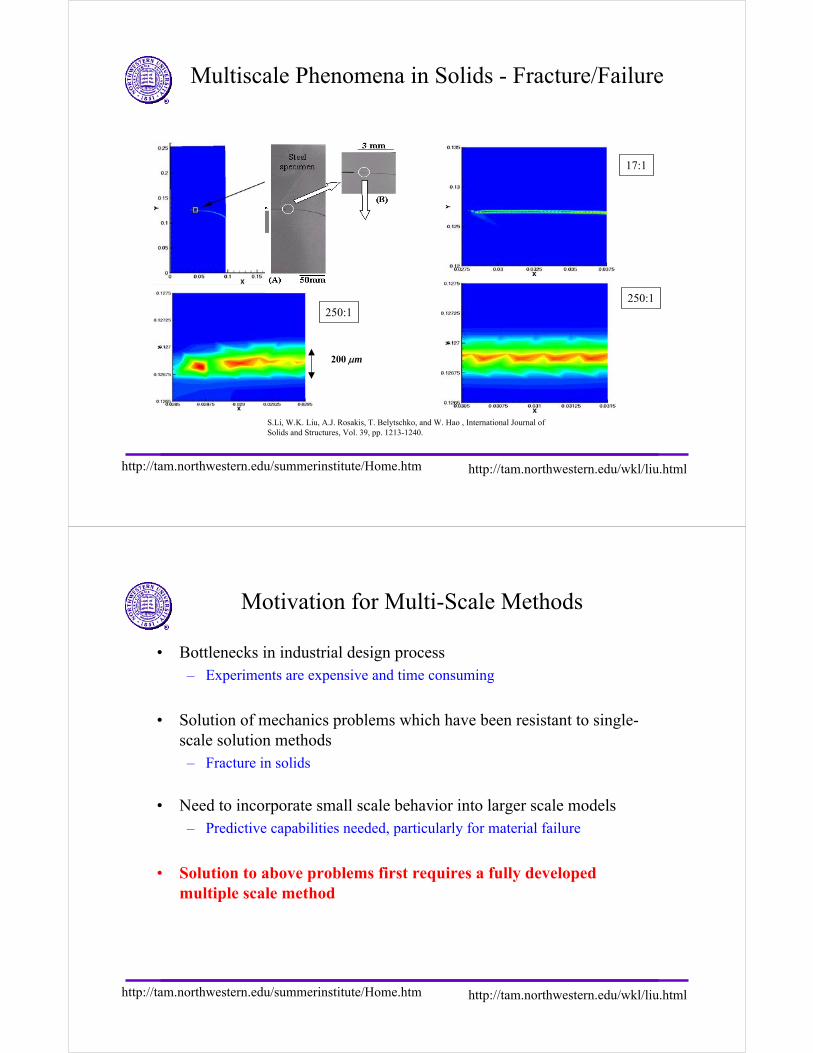
Multiscale Phenomena in Solids - Fracture/Failure
17:1
250:1250:1
200 µm
S.Li, W.K. Liu, A.J. Rosakis, T. Belytschko, and W. Hao , International Journal of Solids and Structures, Vol. 39, pp. 1213-1240.
http://tam.northwestern.edu/summerinstitute/Home.htm http://tam.northwestern.edu/wkl/liu.html
Motivation for Multi-Scale Methods
• Bottlenecks in industrial design process– Experiments are expensive and time consuming
• Solution of mechanics problems which have been resistant to single-scale solution methods– Fracture in solids
• Need to incorporate small scale behavior into larger scale models– Predictive capabilities needed, particularly for material failure
• Solution to above problems first requires a fully developed multiple scale method
http://tam.northwestern.edu/summerinstitute/Home.htm http://tam.northwestern.edu/wkl/liu.html
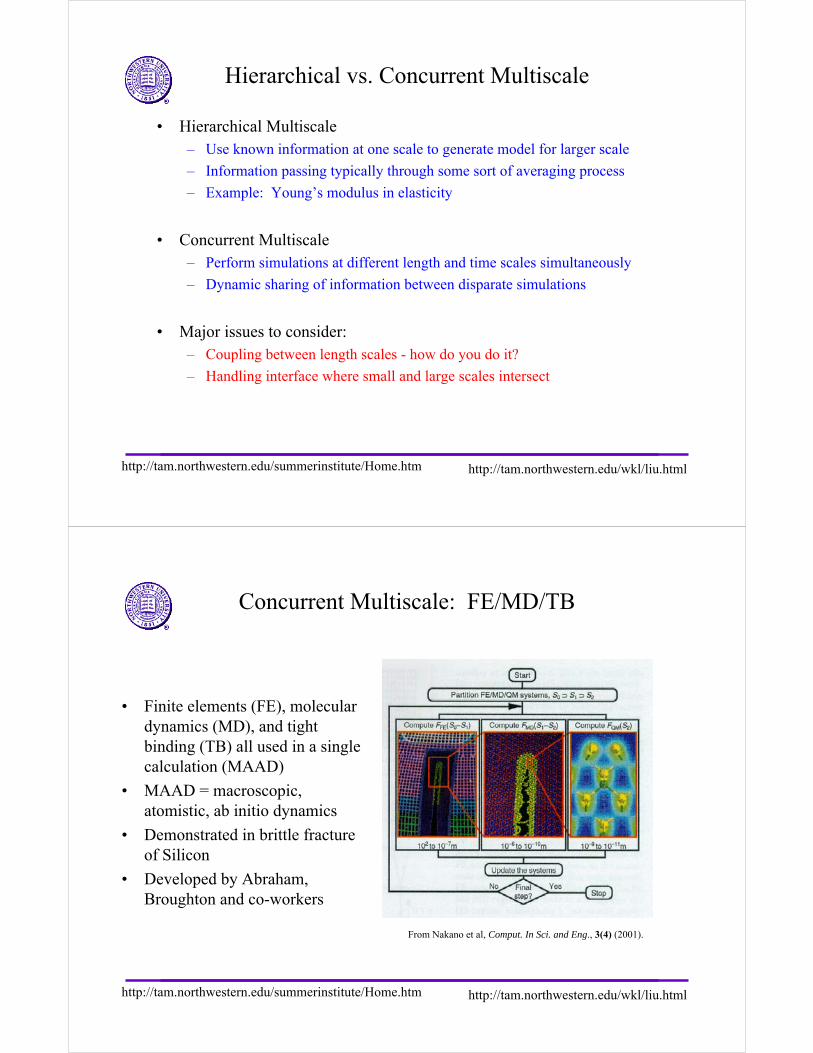
Hierarchical vs. Concurrent Multiscale
• Hierarchical Multiscale– Use known information at one scale to generate model for larger scale
– Information passing typically through some sort of averaging process
– Example: Young’s modulus in elasticity
• Concurrent Multiscale– Perform simulations at different length and time scales simultaneously
– Dynamic sharing of information between disparate simulations
• Major issues to consider:– Coupling between length scales - how do you do it?
– Handling interface where small and large scales intersect
http://tam.northwestern.edu/summerinstitute/Home.htm http://tam.northwestern.edu/wkl/liu.html
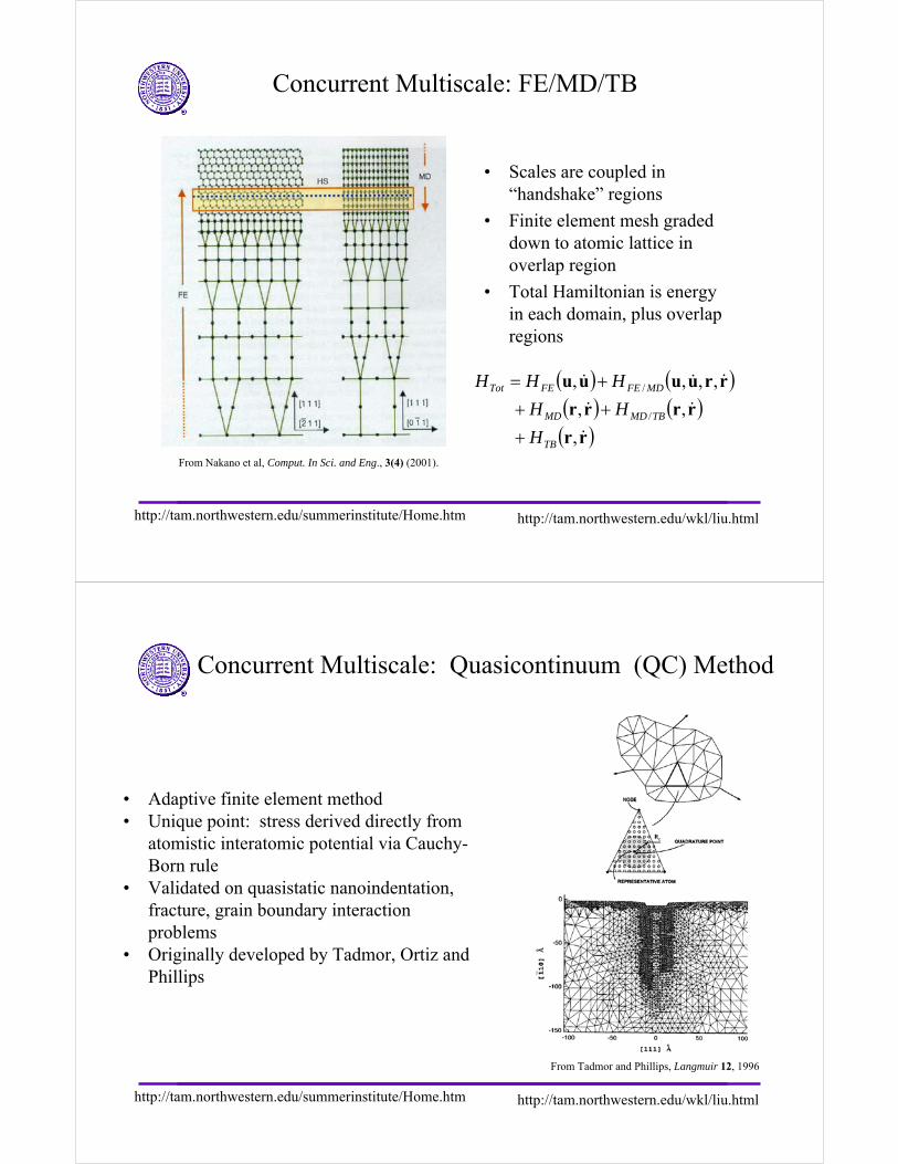
Concurrent Multiscale: FE/MD/TB
• Finite elements (FE), molecular dynamics (MD), and tight binding (TB) all used in a single calculation (MAAD)
• MAAD = macroscopic, atomistic, ab initio dynamics
• Demonstrated in brittle fracture of Silicon
• Developed by Abraham, Broughton and co-workers
From Nakano et al, Comput. In Sci. and Eng., 3(4) (2001).
http://tam.northwestern.edu/summerinstitute/Home.htm http://tam.northwestern.edu/wkl/liu.html
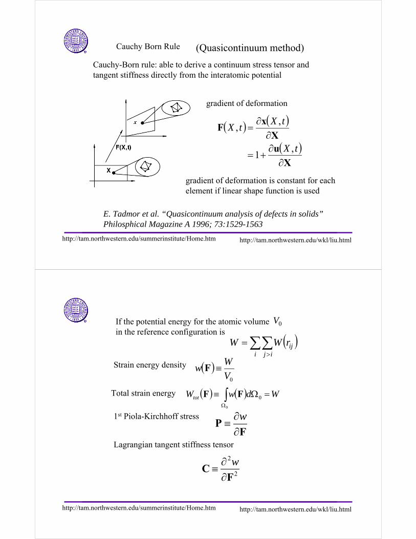
Concurrent Multiscale: FE/MD/TB
• Scales are coupled in “handshake” regions
• Finite element mesh graded down to atomic lattice in overlap region
• Total Hamiltonian is energy in each domain, plus overlap regions
( ) ( )( ) ( )
( )rr
rrrr
rruuuu
&
&&
&&&
,
,,
,,,,
/
/
TB
TBMDMD
MDFEFETot
H
HH
HHH
++++=
From Nakano et al, Comput. In Sci. and Eng., 3(4) (2001).
http://tam.northwestern.edu/summerinstitute/Home.htm http://tam.northwestern.edu/wkl/liu.html
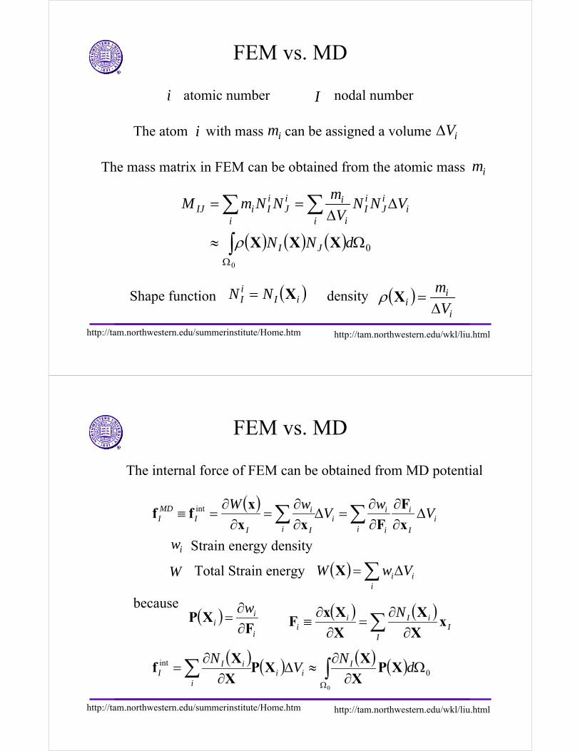
Concurrent Multiscale: Quasicontinuum (QC) Method
From Tadmor and Phillips, Langmuir 12, 1996
• Adaptive finite element method• Unique point: stress derived directly from
atomistic interatomic potential via Cauchy-Born rule
• Validated on quasistatic nanoindentation, fracture, grain boundary interaction problems
• Originally developed by Tadmor, Ortiz and Phillips
http://tam.northwestern.edu/summerinstitute/Home.htm http://tam.northwestern.edu/wkl/liu.html
(Quasicontinuum method)
Cauchy-Born rule: able to derive a continuum stress tensor and tangent stiffness directly from the interatomic potential
gradient of deformation
( ) ( )
( )X
uX
xF
∂∂
+=
∂∂
=
tX
tXtX
,1
,,
gradient of deformation is constant for each element if linear shape function is used
E. Tadmor et al. “Quasicontinuum analysis of defects in solids” Philosphical Magazine A 1996; 73:1529-1563
Cauchy Born Rule
http://tam.northwestern.edu/summerinstitute/Home.htm http://tam.northwestern.edu/wkl/liu.html
FP
∂∂
≡w
2
2
FC
∂∂
≡w
Lagrangian tangent stiffness tensor
1st Piola-Kirchhoff stress
If the potential energy for the atomic volume in the reference configuration is
( )∑∑>
=i ij
ijrWW
Strain energy density ( )0V
Ww ≡F
0V
Total strain energy ( ) ( ) WdwWtot =Ω≡ ∫Ω0
0FF
http://tam.northwestern.edu/summerinstitute/Home.htm http://tam.northwestern.edu/wkl/liu.html
FEM vs. MD
( ) ( ) ( )∫
∑∑
Ω
Ω≈
∆∆
==
0
0dNN
VNNV
mNNmM
JI
ii
iJ
iI
i
i
i
iJ
iIiIJ
XXXρ
The atom with mass can be assigned a volumeim iV∆i
i atomic number I nodal number
The mass matrix in FEM can be obtained from the atomic mass
Shape function ( )iIiI NN X= density ( )
i
ii V
m
∆=Xρ
im
http://tam.northwestern.edu/summerinstitute/Home.htm http://tam.northwestern.edu/wkl/liu.html
FEM vs. MD
( )i
I
i
i i
ii
i I
i
II
MDI V
wV
wW∆
∂∂
∂∂
=∆∂∂
=∂
∂=≡ ∑∑ x
F
Fxx
xff int
( )i
ii
w
FXP
∂∂
= ( ) ( )∑ ∂∂
=∂
∂≡
II
iIii
Nx
X
X
X
XxF
because
( ) ( ) ( ) ( )∫∑Ω
Ω∂
∂≈∆
∂∂
=0
0int d
NV
N Iii
i
iII XP
X
XXP
X
Xf
The internal force of FEM can be obtained from MD potential
Strain energy densityiw
Total Strain energyW ( ) ii
i VwW ∆= ∑X
http://tam.northwestern.edu/summerinstitute/Home.htm http://tam.northwestern.edu/wkl/liu.html
( ) ( )0
0
Ω∂
∂⎟⎟⎠
⎞⎜⎜⎝
⎛∂
∂−= ∫
Ω
dwN
MT
III F
F
X
Xd&&
( )i
iiW
mx
xx
∂∂
−=&&
FEM
MD
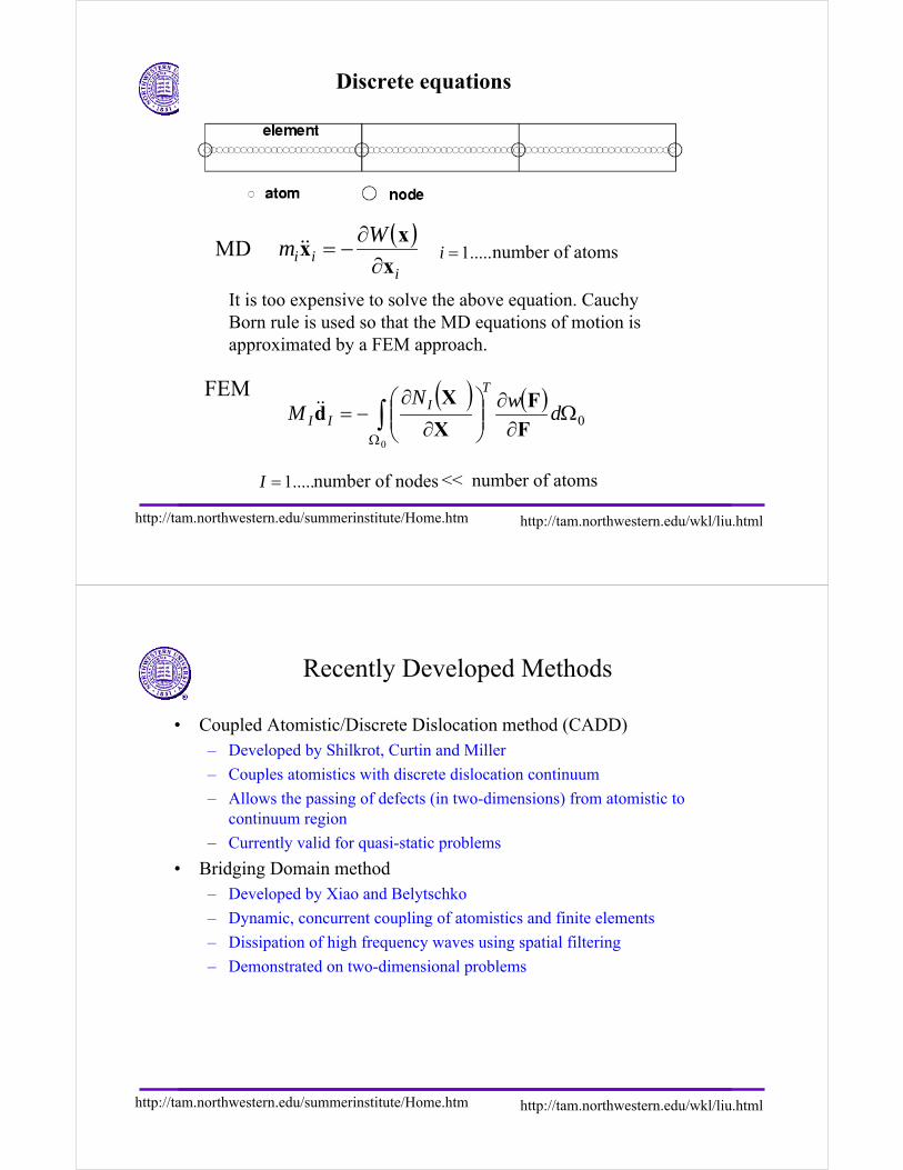
Discrete equations
.....1=i number of atoms
It is too expensive to solve the above equation. Cauchy Born rule is used so that the MD equations of motion is approximated by a FEM approach.
.....1=I number of nodes << number of atoms
http://tam.northwestern.edu/summerinstitute/Home.htm http://tam.northwestern.edu/wkl/liu.html
Recently Developed Methods
• Coupled Atomistic/Discrete Dislocation method (CADD)– Developed by Shilkrot, Curtin and Miller
– Couples atomistics with discrete dislocation continuum
– Allows the passing of defects (in two-dimensions) from atomistic to continuum region
– Currently valid for quasi-static problems
• Bridging Domain method– Developed by Xiao and Belytschko
– Dynamic, concurrent coupling of atomistics and finite elements
– Dissipation of high frequency waves using spatial filtering
– Demonstrated on two-dimensional problems
http://tam.northwestern.edu/summerinstitute/Home.htm http://tam.northwestern.edu/wkl/liu.html
Summary of Multiple Scale Approaches
• Pros:– QC allows full atomistic resolution around defects, crucial atomic regions
– MAAD successfully applied to brittle fracture of silicon
– CADD combines atomistic and discrete dislocation methods, allowing defects to propagate from atomistic to continuum regions
• Cons:– FE region meshed down to atomic scale in MAAD
– No explicit treatment of small scale waves in continuum region in MAAD
– QC and CADD currently limited to quasistatic problems
• Remaining issues:– Need for dynamic, finite temperature multiple scale method
– True coarse scale representation
– Mathematically consistent treatment of high frequency waves emitted from MD region in continuum
http://tam.northwestern.edu/summerinstitute/Home.htm http://tam.northwestern.edu/wkl/liu.html
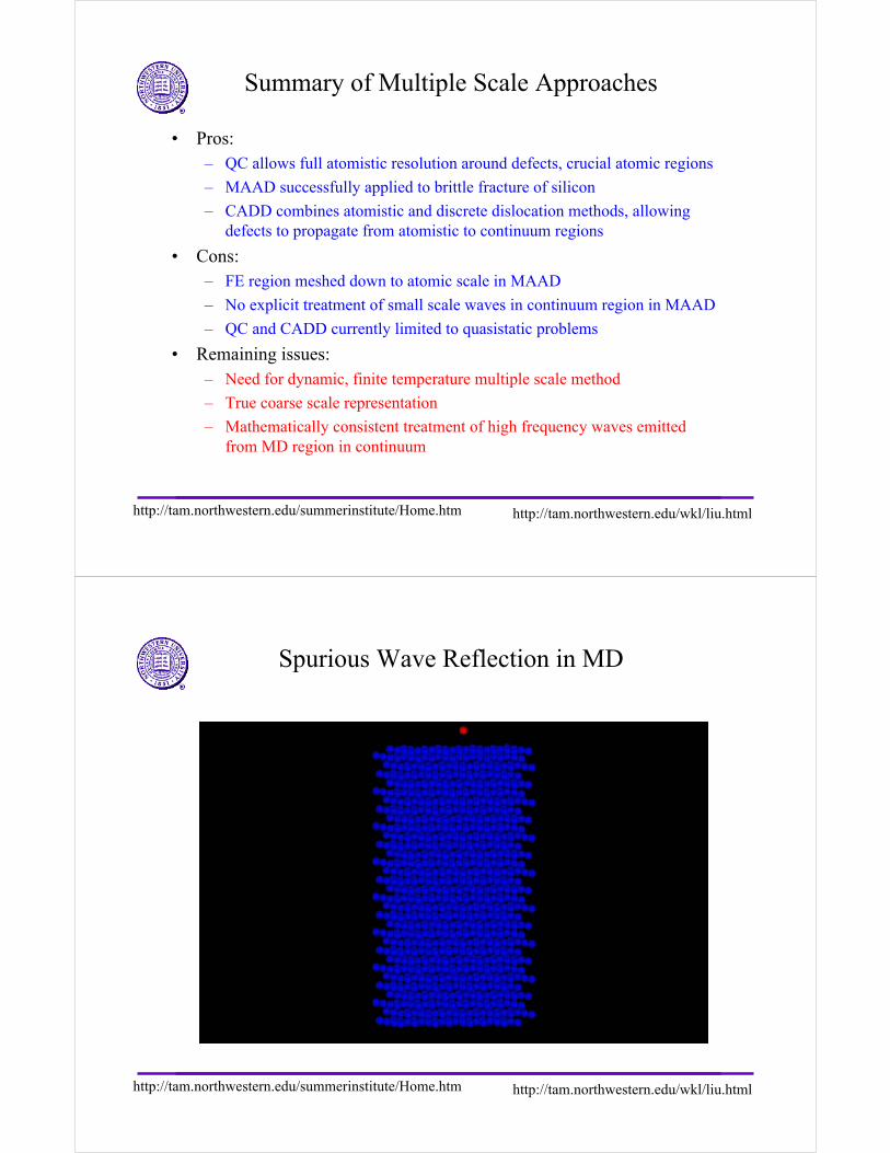
Spurious Wave Reflection in MD
http://tam.northwestern.edu/summerinstitute/Home.htm http://tam.northwestern.edu/wkl/liu.html
Concurrent Multiple Scales: Goals
• Development of method for coupling molecular dynamics to finite element or meshfree computations in concurrent simulations
• Simulation of time dependent, finite temperature problems
• True “coarse scale” continuum discretization -- no meshing down to atomic scale
• Multiple time-stepping algorithms to take advantage of multiple time scales
– don’t want to be limited to nano time scale everywhere in the domain
• Re-use of existing MD and continuum codes
• Easily parallelizable algorithms
http://tam.northwestern.edu/summerinstitute/Home.htm http://tam.northwestern.edu/wkl/liu.html
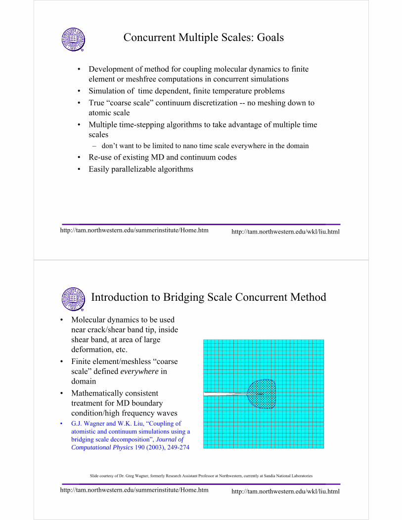
Introduction to Bridging Scale Concurrent Method
• Molecular dynamics to be used near crack/shear band tip, inside shear band, at area of large deformation, etc.
• Finite element/meshless “coarse scale” defined everywhere in domain
• Mathematically consistent treatment for MD boundary condition/high frequency waves
• G.J. Wagner and W.K. Liu, “Coupling of atomistic and continuum simulations using a bridging scale decomposition”, Journal of Computational Physics 190 (2003), 249-274
Slide courtesy of Dr. Greg Wagner, formerly Research Assistant Professor at Northwestern, currently at Sandia National Laboratories
http://tam.northwestern.edu/summerinstitute/Home.htm http://tam.northwestern.edu/wkl/liu.html
Boundary Conditions
• We want to avoid grading the coarse mesh down to the atomic lattice scale
– expensive
– too much information
– limits coarse scale time step
• Information passes from a fine MD lattice directly into a coarse scale mesh
• Main problem: this leads to internal reflection of small-scale waves– small-scale energy can’t be represented on the coarse scale, has nowhere
else to go
http://tam.northwestern.edu/summerinstitute/Home.htm http://tam.northwestern.edu/wkl/liu.html
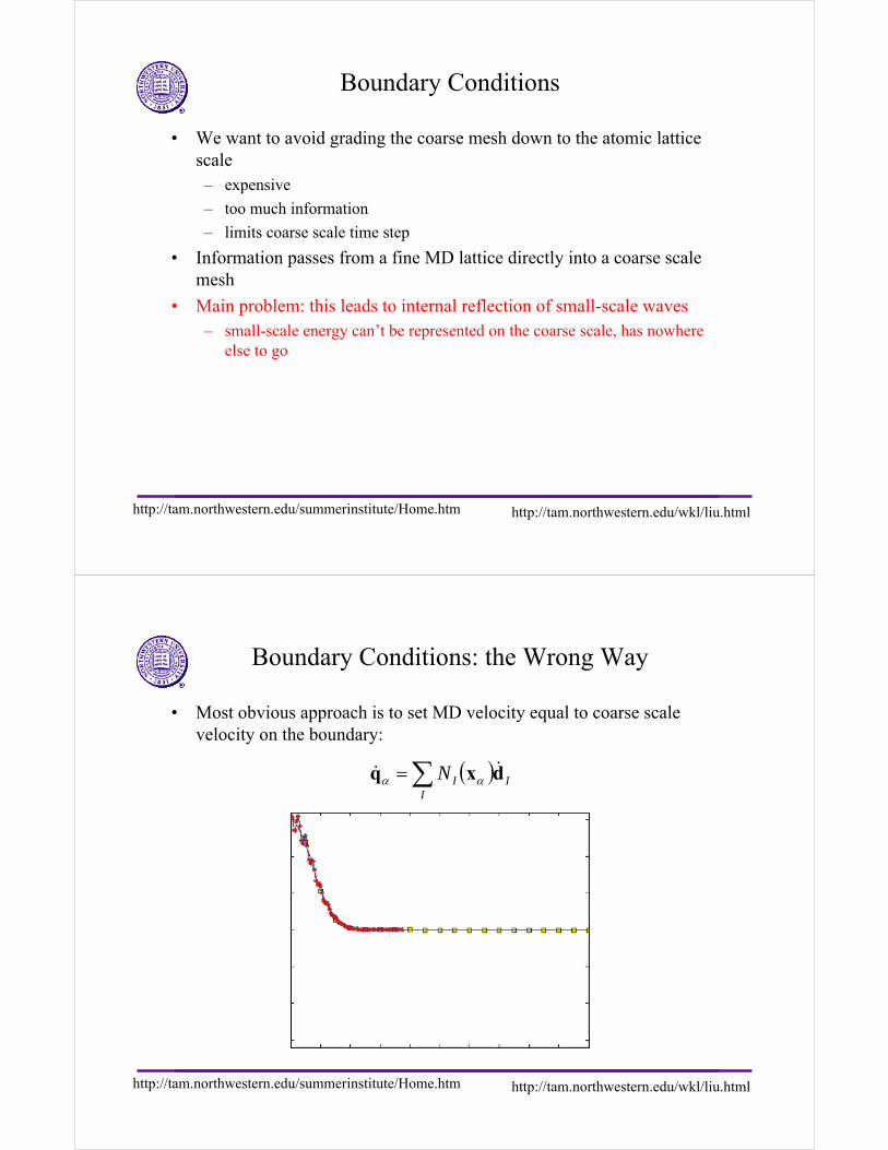
Boundary Conditions: the Wrong Way
• Most obvious approach is to set MD velocity equal to coarse scale velocity on the boundary:
( )∑=I
IIN dxq && αα
http://tam.northwestern.edu/summerinstitute/Home.htm http://tam.northwestern.edu/wkl/liu.html
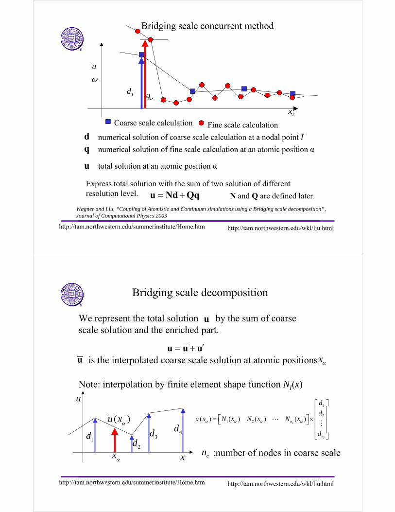
numerical solution of coarse scale calculation at a nodal point I
Wagner and Liu, “Coupling of Atomistic and Continuum simulations using a Bridging scale decomposition”, Journal of Computational Physics 2003
2x
Id
u
ω
qα
Coarse scale calculation Fine scale calculation
dq numerical solution of fine scale calculation at an atomic position α
u total solution at an atomic position α
Bridging scale concurrent method
u Nd Qq= +Express total solution with the sum of two solution of differentresolution level. N and Q are defined later.
http://tam.northwestern.edu/summerinstitute/Home.htm http://tam.northwestern.edu/wkl/liu.html
We represent the total solution by the sum of coarse scale solution and the enriched part.
u
uuu ′+=
Bridging scale decomposition
Note: interpolation by finite element shape function NI(x)
1d2d
3d 4d
x
u1
2
1 2( ) ( ) ( ) ( )c
c
n
n
d
du x N x N x N x
d
α α α α
⎡ ⎤⎢ ⎥⎢ ⎥⎡ ⎤= ×⎣ ⎦ ⎢ ⎥⎢ ⎥⎣ ⎦
LM u (xα )
xα:number of nodes in coarse scalecn
is the interpolated coarse scale solution at atomic positionsu xα
http://tam.northwestern.edu/summerinstitute/Home.htm http://tam.northwestern.edu/wkl/liu.html
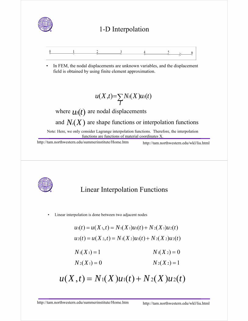
1-D Interpolation
• In FEM, the nodal displacements are unknown variables, and the displacement field is obtained by using finite element approximation.
( , ) ( ) ( )I I
INu X t X u t=∑
where are nodal displacements
and are shape functions or interpolation functions
( )Iu t( )IN X
Note: Here, we only consider Lagrange interpolation functions. Therefore, the interpolation functions are functions of material coordinates X.
http://tam.northwestern.edu/summerinstitute/Home.htm http://tam.northwestern.edu/wkl/liu.html
Linear Interpolation Functions
• Linear interpolation is done between two adjacent nodes
1 1 2 2( , ) ( ) ( ) ( ) ( )u X t N X u t N X u t= +
1 1 1 1 1 2 1 2( ) ( , ) ( ) ( ) ( ) ( )u t u X t N X u t N X u t= = +
2 2 1 2 1 2 2 2( ) ( , ) ( ) ( ) ( ) ( )u t u X t N X u t N X u t= = +
2 1( ) 0N X =
1 1( ) 1N X = 1 2( ) 0N X =
2 2( ) 1N X =
http://tam.northwestern.edu/summerinstitute/Home.htm http://tam.northwestern.edu/wkl/liu.html
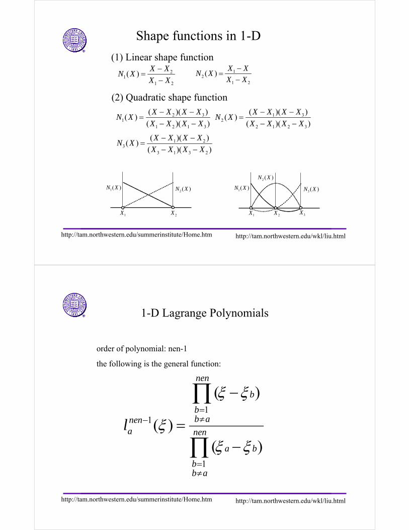
Shape functions in 1-D
(1) Linear shape function2
11 2
( )X X
N XX X
−=
−1
21 2
( )X X
N XX X
−=
−
1 32
2 1 2 3
( )( )( )
( )( )
X X X XN X
X X X X
− −=
− −
(2) Quadratic shape function
2 31
1 2 1 3
( )( )( )
( )( )
X X X XN X
X X X X
− −=
− −
1 23
3 1 3 2
( )( )( )
( )( )
X X X XN X
X X X X
− −=
− −
1( )N X2 ( )N X
1X 2X
1( )N X3( )N X
2 ( )N X
1X 3X2X
http://tam.northwestern.edu/summerinstitute/Home.htm http://tam.northwestern.edu/wkl/liu.html
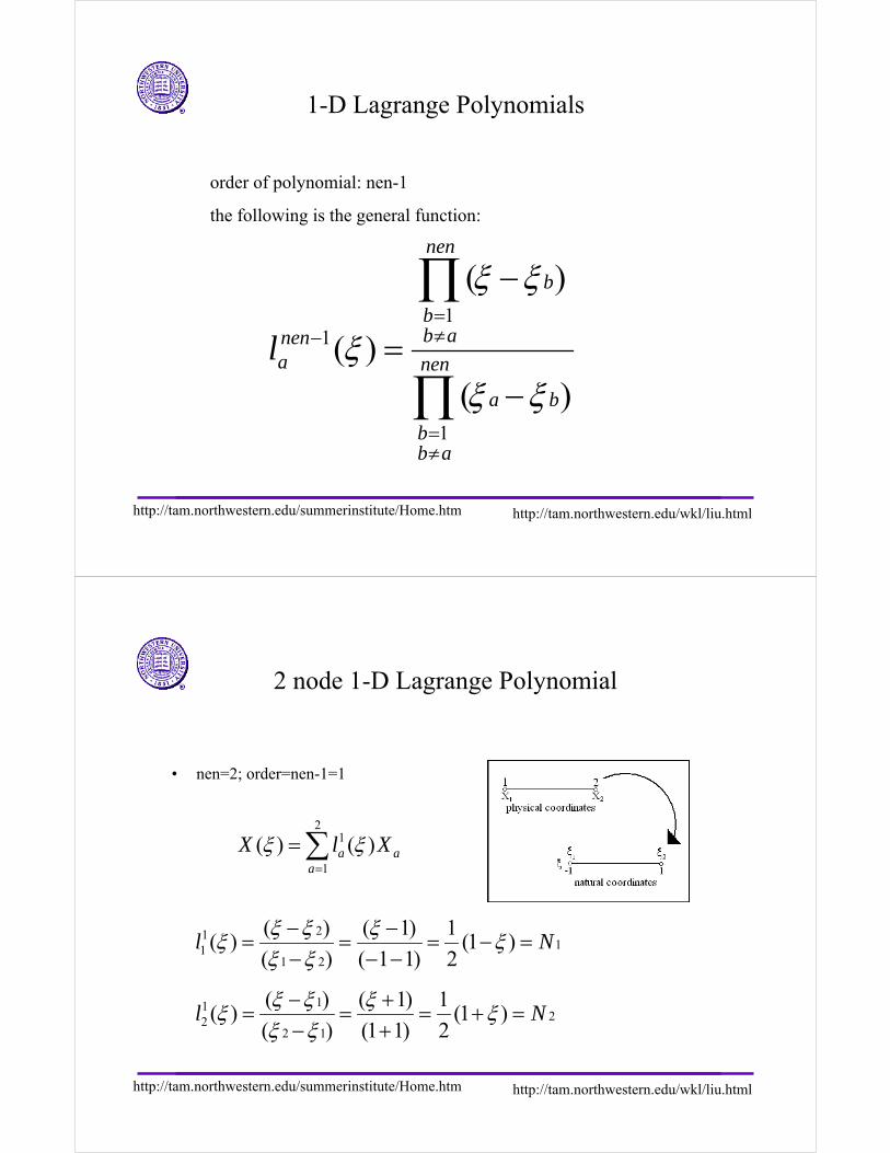
1-D Lagrange Polynomials
11
1
( )
( )( )
nen
b
bb anen
a nen
a b
bb a
l
ξ ξ
ξξ ξ
=≠−
=≠
−
=−
∏
∏
order of polynomial: nen-1
the following is the general function:
http://tam.northwestern.edu/summerinstitute/Home.htm http://tam.northwestern.edu/wkl/liu.html
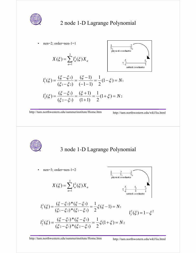
2 node 1-D Lagrange Polynomial
• nen=2; order=nen-1=1
2111
1 2
( ) ( 1) 1( ) (1 )
( ) ( 1 1) 2l N
ξ ξ ξξ ξξ ξ
− −= = = − =
− − −
1122
2 1
( ) ( 1) 1( ) (1 )
( ) (1 1) 2l N
ξ ξ ξξ ξξ ξ
− += = = + =
− +
21
1
( ) ( )a aa
X l Xξ ξ=
= ∑
http://tam.northwestern.edu/summerinstitute/Home.htm http://tam.northwestern.edu/wkl/liu.html
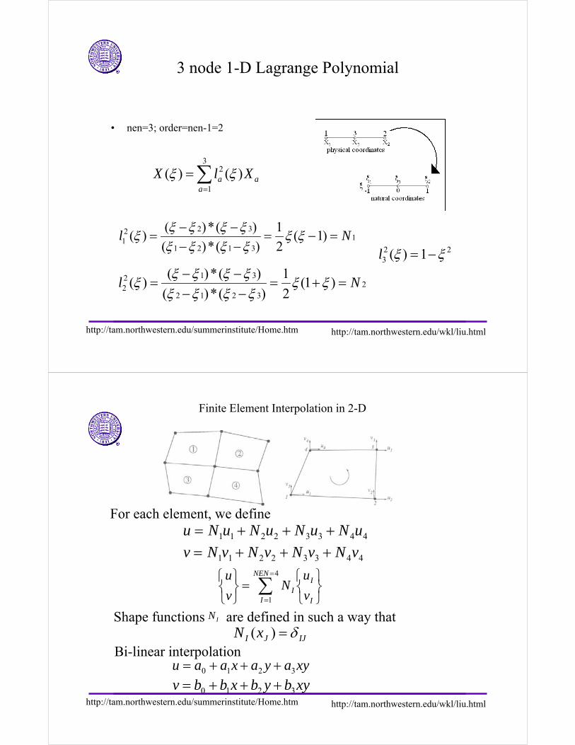
3 node 1-D Lagrange Polynomial
• nen=3; order=nen-1=2
2 3211
1 2 1 3
( )*( ) 1( ) ( 1)
( )*( ) 2l N
ξ ξ ξ ξξ ξ ξξ ξ ξ ξ
− −= = − =
− −
1 3222
2 1 2 3
( )*( ) 1( ) (1 )
( )*( ) 2l N
ξ ξ ξ ξξ ξ ξξ ξ ξ ξ
− −= = + =
− −
32
1
( ) ( )a aa
X l Xξ ξ=
= ∑
2 23 ( ) 1l ξ ξ= −
http://tam.northwestern.edu/summerinstitute/Home.htm http://tam.northwestern.edu/wkl/liu.html
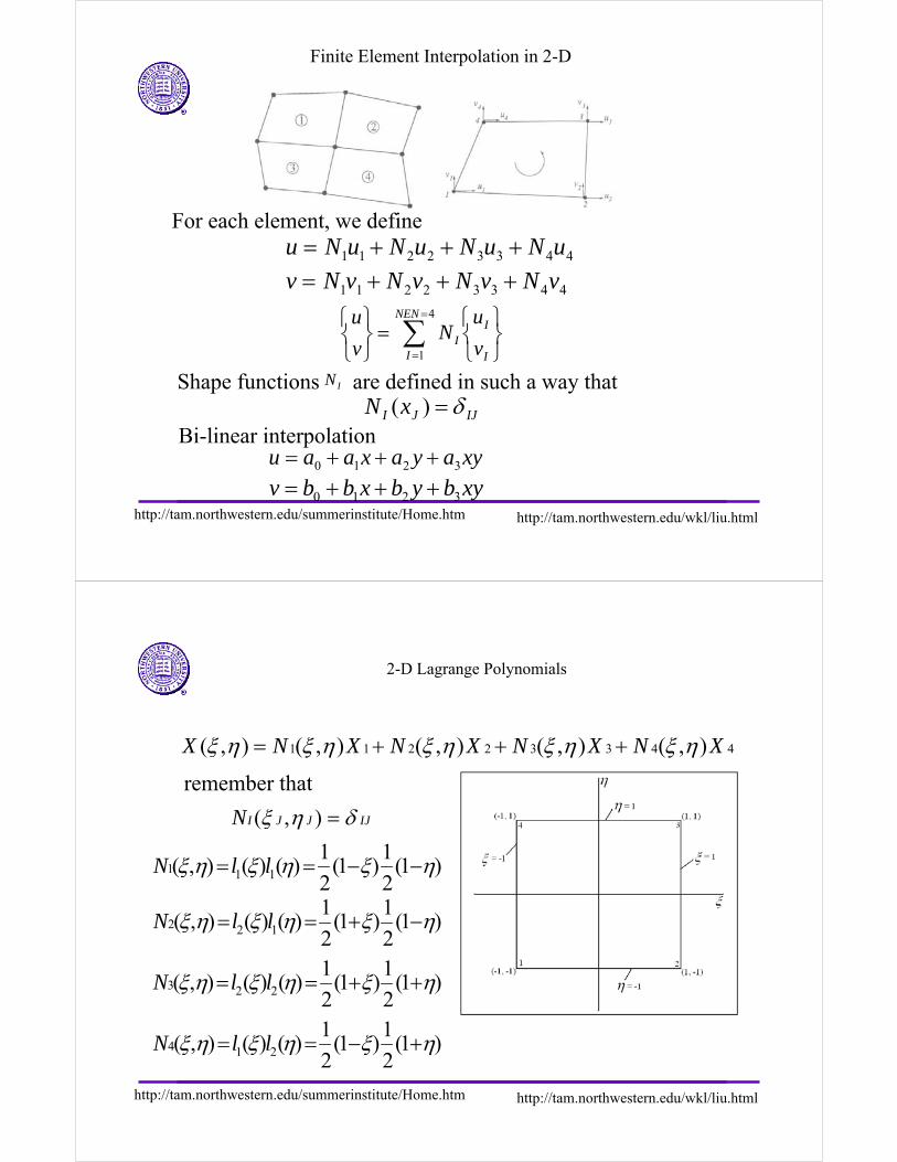
Finite Element Interpolation in 2-D
For each element, we define
44332211 uNuNuNuNu +++=
44332211 vNvNvNvNv +++=
∑=
= ⎭⎬⎫
⎩⎨⎧
=⎭⎬⎫
⎩⎨⎧ 4
1
NEN
I I
II v
uN
v
u
Shape functions are defined in such a way thatIN
IJJI xN δ=)(Bi-linear interpolation
xyayaxaau 3210 +++=xybybxbbv 3210 +++=
http://tam.northwestern.edu/summerinstitute/Home.htm http://tam.northwestern.edu/wkl/liu.html
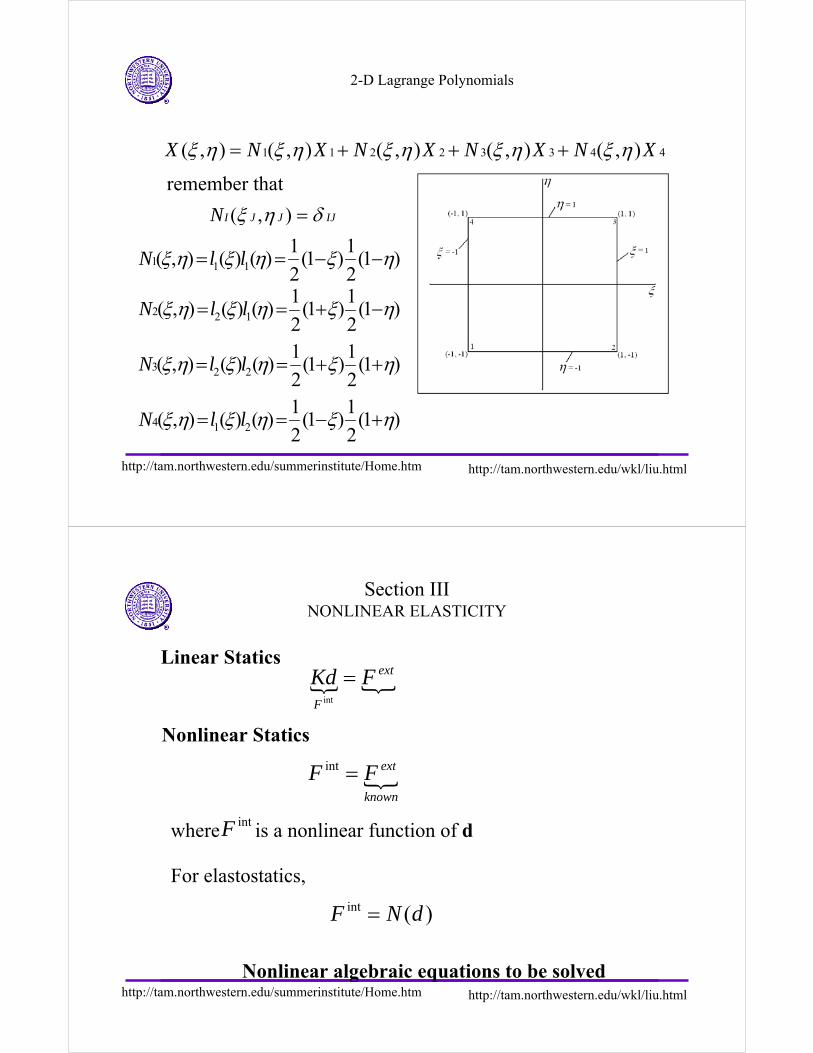
2-D Lagrange Polynomials
1 1 2 2 3 3 4 4( , ) ( , ) ( , ) ( , ) ( , )X N X N X N X N Xξ η ξ η ξ η ξ η ξ η= + + +
remember that
( , )I J J IJN ξ η δ=
1 1 1
1 1( , ) ( ) ( ) (1 ) (1 )
2 2N l lξ η ξ η ξ η= = − −
2 2 1
1 1( , ) ( ) ( ) (1 ) (1 )
2 2N l lξ η ξ η ξ η= = + −
3 2 2
1 1( , ) ( ) ( ) (1 ) (1 )
2 2N l lξ η ξ η ξ η= = + +
4 1 2
1 1( , ) ( ) ( ) (1 ) (1 )
2 2N l lξ η ξ η ξ η= = − +
http://tam.northwestern.edu/summerinstitute/Home.htm http://tam.northwestern.edu/wkl/liu.html
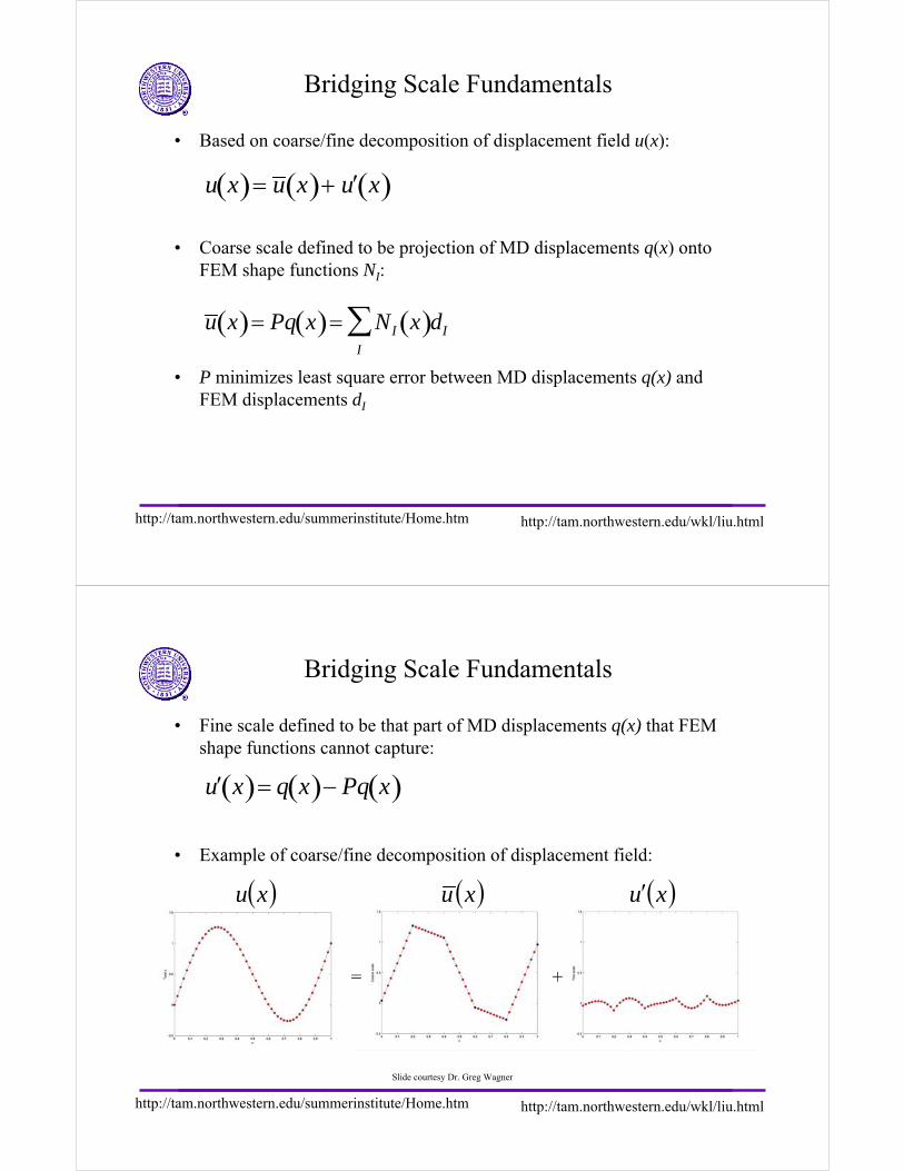
Bridging Scale Fundamentals
• Based on coarse/fine decomposition of displacement field u(x):
• Coarse scale defined to be projection of MD displacements q(x) onto FEM shape functions NI:
• P minimizes least square error between MD displacements q(x) and FEM displacements dI
u x( )= u x( )+ ′ u x( )
u x( )= Pq x( )= NI x( )dI
I
∑
http://tam.northwestern.edu/summerinstitute/Home.htm http://tam.northwestern.edu/wkl/liu.html
Bridging Scale Fundamentals
• Fine scale defined to be that part of MD displacements q(x) that FEM shape functions cannot capture:
• Example of coarse/fine decomposition of displacement field:
′ u x( )= q x( )− Pq x( )
= +
( )xu ( )xu ( )xu′
Slide courtesy Dr. Greg Wagner
http://tam.northwestern.edu/summerinstitute/Home.htm http://tam.northwestern.edu/wkl/liu.html
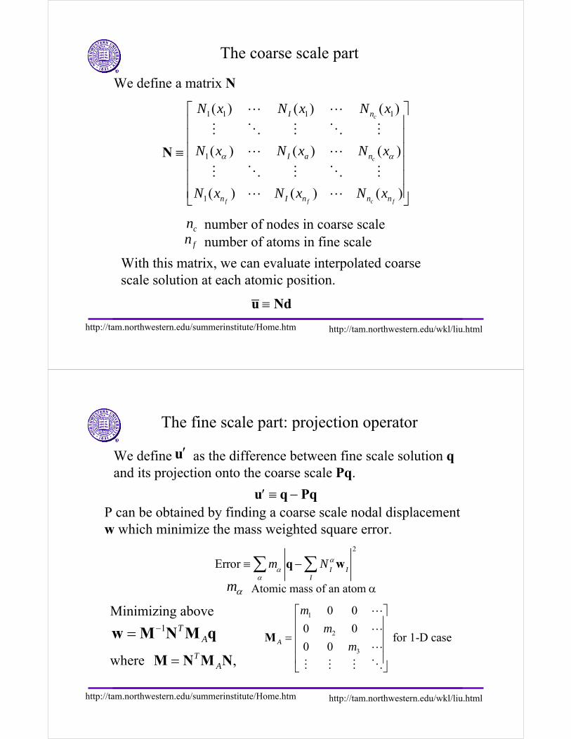
The coarse scale part
With this matrix, we can evaluate interpolated coarse scale solution at each atomic position.
1 1 1 1
1
1
( ) ( ) ( )
( ) ( ) ( )
( ) ( ) ( )
N
c
c
f f c f
I n
I a n
n I n n n
N x N x N x
N x N x N x
N x N x N x
α α
⎡ ⎤⎢ ⎥⎢ ⎥⎢ ⎥≡⎢ ⎥⎢ ⎥⎢ ⎥⎣ ⎦
L L
M O M O M
L L
M O M O M
L L
We define a matrix N
number of nodes in coarse scalenumber of atoms in fine scalefn
cn
u ≡ Nd
http://tam.northwestern.edu/summerinstitute/Home.htm http://tam.northwestern.edu/wkl/liu.html
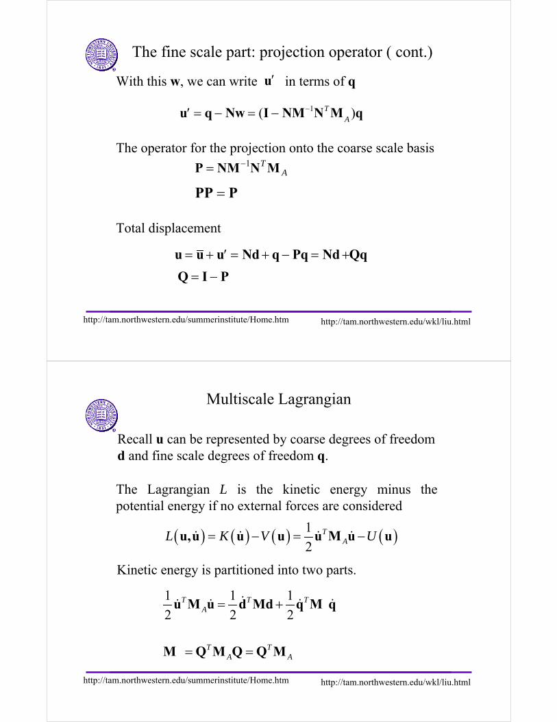
We define as the difference between fine scale solution qand its projection onto the coarse scale Pq.
Minimizing above
qMNMw AT1−=
αm Atomic mass of an atom α
,NMNM AT=
u′
The fine scale part: projection operator
P can be obtained by finding a coarse scale nodal displacement w which minimize the mass weighted square error.
where
′u ≡ q − Pq
Error ≡ mα q − NIα w
II
∑2
α∑
1
2
3
0 0
0 0for 1-D case
0 0M A
m
m
m
⎡ ⎤⎢ ⎥⎢ ⎥=⎢ ⎥⎢ ⎥⎣ ⎦
L
L
L
M M M O
http://tam.northwestern.edu/summerinstitute/Home.htm http://tam.northwestern.edu/wkl/liu.html
With this w, we can write in terms of q
AT MNNMP 1−=
The operator for the projection onto the coarse scale basis
PPP =
Total displacement
The fine scale part: projection operator ( cont.)
u′
′u = q − Nw = (I − NM−1NT MA)q
u = u + ′u = Nd + q − Pq = Nd +Qq
Q = I − P
http://tam.northwestern.edu/summerinstitute/Home.htm http://tam.northwestern.edu/wkl/liu.html
Recall u can be represented by coarse degrees of freedomd and fine scale degrees of freedom q.
The Lagrangian L is the kinetic energy minus the potential energy if no external forces are considered
Multiscale Lagrangian
Kinetic energy is partitioned into two parts.
( ) ( ) ( ) ( )1
2u,u u u u M u uT
AL K V U= − = −& & & &
1 1 1
2 2 2T T T
A = +u M u d Md q q& & && & M
T TA A= =Q M Q Q MM
http://tam.northwestern.edu/summerinstitute/Home.htm http://tam.northwestern.edu/wkl/liu.html
u
uuuf
∂∂
−≡′+)(
)(U
Multiscale equations of motion
d0
d
d0
d
L L
t
L L
t
⎧ ∂ ∂⎛ ⎞ − =⎜ ⎟⎪ ∂ ∂⎝ ⎠⎪⎨
⎛ ⎞∂ ∂⎪ − =⎜ ⎟⎪ ∂ ∂⎝ ⎠⎩
d d
q q
&
&
We can obtain equations of motion by
( )
( )
( ) ( )
( ) ( )
T T
T T T
U U
U U
⎧ ∂ ∂ ∂ ′= − = − = + = +⎪ ∂ ∂ ∂⎪⎨ ∂ ∂ ∂⎪ ′= − = − = + = +⎪ ∂ ∂ ∂⎩
d,q uΜd N f u u N f Nd Qq
d u dd,q u
q Q N f u u Q f Nd Qqq u q
&&
&&M
Substituting the expression for the multiscale Lagrangian into the above equations gives
where
( ) ( ) ( )1 1,
2 2u u d,d,q,q d Μd q q d,qT TL L U= = + −& & && & && M
http://tam.northwestern.edu/summerinstitute/Home.htm http://tam.northwestern.edu/wkl/liu.html
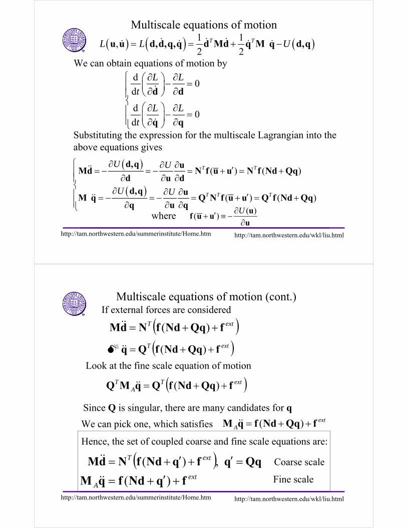
If external forces are considered
( )extT fQqNdfNdΜ ++= )(&&
( )extT fQqNdfQq ++= )(&&
( )extTA
T fQqNdfQqMQ ++= )(&&
extA fQqNdfqM ++= )(&&
Since Q is singular, there are many candidates for q
We can pick one, which satisfies
Multiscale equations of motion (cont.)
Look at the fine scale equation of motion
Hence, the set of coupled coarse and fine scale equations are:
( ) QqqfqNdfNdΜ =′+′+= ,)( extT&&
extA fqNdfqM +′+= )(&&
Coarse scale
Fine scale
http://tam.northwestern.edu/summerinstitute/Home.htm http://tam.northwestern.edu/wkl/liu.html
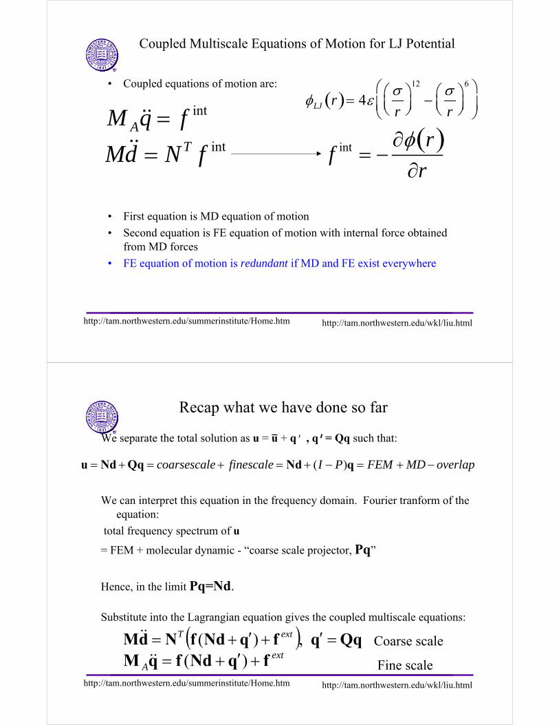
Coupled Multiscale Equations of Motion for LJ Potential
• Coupled equations of motion are:
• First equation is MD equation of motion
• Second equation is FE equation of motion with internal force obtained from MD forces
• FE equation of motion is redundant if MD and FE exist everywhere
intAM q f=&&
intTMd N f=&& f int = −∂φ r( )
∂r
φLJ r( )= 4εσr
⎛⎝⎜
⎞⎠⎟
12
−σr
⎛⎝⎜
⎞⎠⎟
6⎛
⎝⎜
⎞
⎠⎟
http://tam.northwestern.edu/summerinstitute/Home.htm http://tam.northwestern.edu/wkl/liu.html
Recap what we have done so far
We separate the total solution as u = u + q’ , q’= Qq such that:
We can interpret this equation in the frequency domain. Fourier tranform of the equation:
total frequency spectrum of u
= FEM + molecular dynamic - “coarse scale projector, Pq”
Hence, in the limit Pq=Nd.
Substitute into the Lagrangian equation gives the coupled multiscale equations:
( )u Nd Qq Nd qcoarsescale finescale I P FEM MD overlap= + = + = + − = + −
( ) QqqfqNdfNdΜ =′+′+= ,)( extT&&ext
A fqNdfqM +′+= )(&&Coarse scale
Fine scale
http://tam.northwestern.edu/summerinstitute/Home.htm http://tam.northwestern.edu/wkl/liu.html
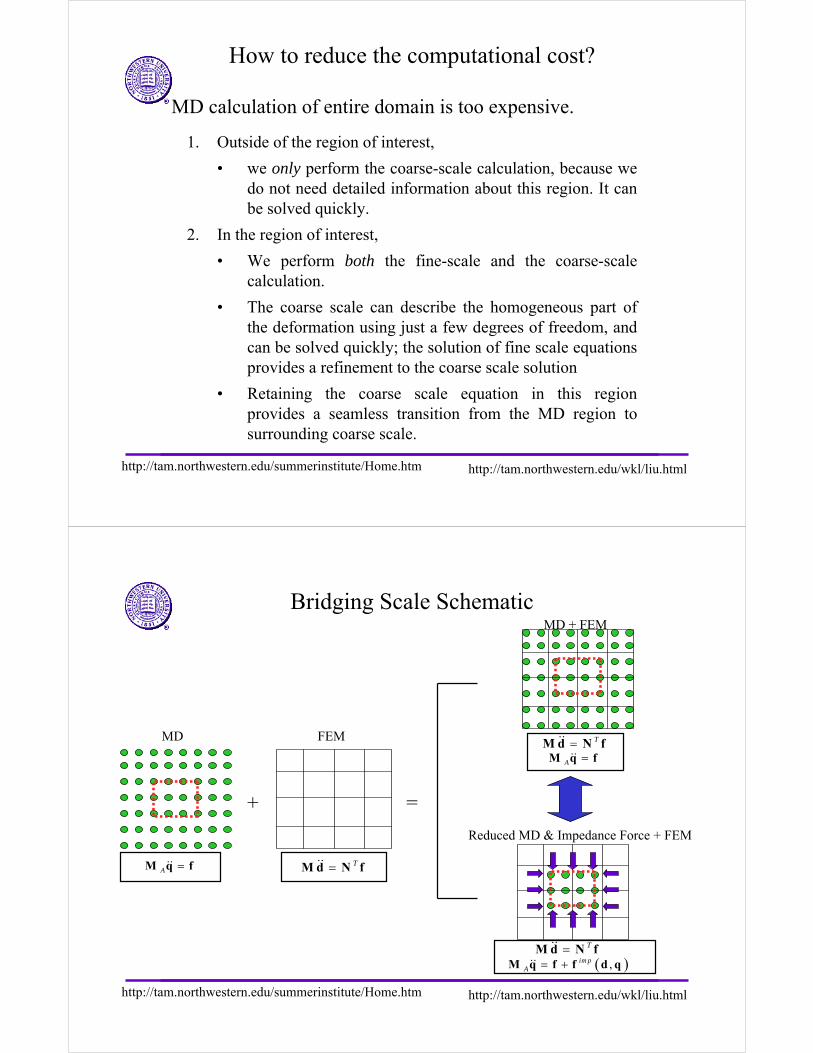
1. Outside of the region of interest,
• we only perform the coarse-scale calculation, because we do not need detailed information about this region. It can be solved quickly.
2. In the region of interest,
• We perform both the fine-scale and the coarse-scale calculation.
• The coarse scale can describe the homogeneous part of the deformation using just a few degrees of freedom, and can be solved quickly; the solution of fine scale equations provides a refinement to the coarse scale solution
• Retaining the coarse scale equation in this region provides a seamless transition from the MD region to surrounding coarse scale.
How to reduce the computational cost?
MD calculation of entire domain is too expensive.
http://tam.northwestern.edu/summerinstitute/Home.htm http://tam.northwestern.edu/wkl/liu.html
Bridging Scale Schematic
+ =
MD FEM
M q fA =&& M d N fT=&&
MD + FEM
Reduced MD & Impedance Force + FEM
M d N fT=&&
( ),M q f f d qim pA = +&&
M d N fT=&&
M q fA =&&
http://tam.northwestern.edu/summerinstitute/Home.htm http://tam.northwestern.edu/wkl/liu.html
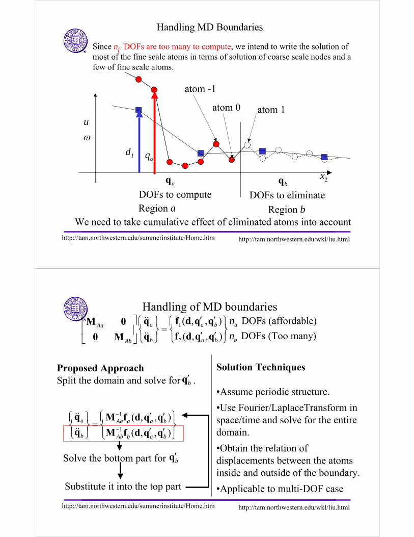
Since nf DOFs are too many to compute, we intend to write the solution of most of the fine scale atoms in terms of solution of coarse scale nodes and a few of fine scale atoms.
Id qα
u
ω
atom -1
atom 0 atom 1
We need to take cumulative effect of eliminated atoms into account
2x
Handling MD Boundaries
bqaq
DOFs to compute DOFs to eliminateRegion a Region b
http://tam.northwestern.edu/summerinstitute/Home.htm http://tam.northwestern.edu/wkl/liu.html
Handling of MD boundaries DOFs (affordable)an
DOFs (Too many)bn1
2
( , , )
( , , )a a bAa
b a bAb
′ ′⎡ ⎤ ⎧ ⎫ ⎧ ⎫=⎨ ⎬ ⎨ ⎬⎢ ⎥ ′ ′⎩ ⎭ ⎩ ⎭⎣ ⎦
q f d q qM 0
q f d q q0 M
&&
&&
Proposed ApproachSplit the domain and solve for .
1
1
( , , )
( , , )a Aa a a b
b Ab b a b
−
−
′ ′⎧ ⎫⎧ ⎫=⎨ ⎬ ⎨ ⎬′ ′⎩ ⎭ ⎩ ⎭
q M f d q q
q M f d q q
&&
&&
Solve the bottom part for b′q
Substitute it into the top part
b′qSolution Techniques
•Assume periodic structure.
•Use Fourier/LaplaceTransform in space/time and solve for the entire domain.
•Obtain the relation of displacements between the atoms inside and outside of the boundary.
•Applicable to multi-DOF case
http://tam.northwestern.edu/summerinstitute/Home.htm http://tam.northwestern.edu/wkl/liu.html
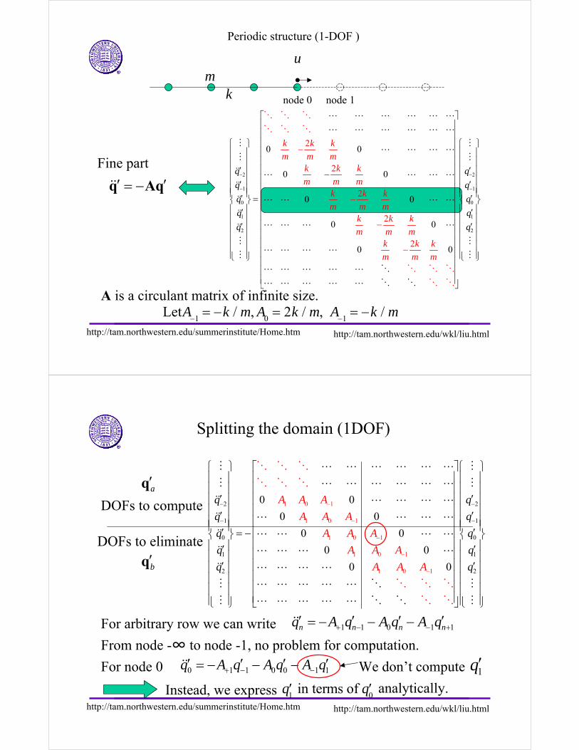
Periodic structure (1-DOF )
A is a circulant matrix of infinite size.
um
k node 0 node 1
qAq ′−=′&&
A−1= −k / m, A
0= 2k / m, A−1
= −k / mLet
Fine part2
1
0
1
2
2
2
2
2
2
0 0
0 0
0 0
0 0
0 0
k k k
m m mk k k
m m mk k k
m m mk k k
m m mk k k
m
q
q
q
m
q
q
m
−
−
⎡ ⎤⎢ ⎥⎢ ⎥⎢ ⎥⎧ ⎫⎢ ⎥⎪ ⎪⎢ ⎥⎪ ⎪
′ ⎢ ⎥⎪ ⎪⎢ ⎥⎪ ⎪′ ⎢ ⎥⎪ ⎪⎪ ⎪ ⎢ ⎥′ =⎨ ⎬⎢ ⎥⎪ ⎪′ ⎢⎪ ⎪⎢′⎪ ⎪⎢⎪ ⎪⎢⎪ ⎪⎢⎪ ⎪⎩ ⎭ ⎢⎢⎢⎣ ⎦
−
−
−
−
−
L L L L L L
L L L L L L
ML L L L
M
&& L L L L&&
&& L L L L
&&
L L L L&&
ML L L L
M
L L L L L O
L L L L
O O O
O O O
O O
O
O
OO OL
2
1
0
1
2
q
q
q
q
q
−
−
⎧ ⎫⎪ ⎪⎪ ⎪
′⎪ ⎪⎪ ⎪′⎪ ⎪⎪ ⎪′⎨ ⎬⎪ ⎪′⎥ ⎪ ⎪
⎥ ′⎪ ⎪⎥ ⎪ ⎪⎥ ⎪ ⎪⎥ ⎪ ⎪⎩ ⎭⎥⎥⎥
M
M
M
M
http://tam.northwestern.edu/summerinstitute/Home.htm http://tam.northwestern.edu/wkl/liu.html
Splitting the domain (1DOF)
Instead, we express ′q1 in terms of ′q
0
2 2
1
0
1
2
1 0 1
1 0 1
1 0 1
1 0 1
1 0 1
0 0
0 0
0 0
0 0
0 0
A A A
A A A
A A A
A A A
A A
q q
q q
q
q
q A
−
−
−
−
− −
−
−
⎧ ⎫ ⎡ ⎤⎪ ⎪ ⎢ ⎥⎪ ⎪ ⎢ ⎥
′ ′⎪ ⎪ ⎢ ⎥⎪ ⎪ ⎢ ⎥′ ′⎪ ⎪ ⎢ ⎥⎪ ⎪′ ⎢ ⎥= −⎨ ⎬
⎢ ⎥⎪ ⎪′ ⎢ ⎥⎪ ⎪⎢ ⎥′⎪ ⎪⎢ ⎥⎪ ⎪⎢ ⎥⎪ ⎪⎢ ⎥⎪ ⎪⎩ ⎭ ⎣ ⎦
M L L L L L L M
M L L L L L L M
&& L L L L
&& L L L L
&& L L L L
&& L L L L
&& L L L L
M L L L L L O
M L L L
O O O
O O O
O O
O O OL L O
O
1
0
1
2
q
q
q
−
⎧ ⎫⎪ ⎪⎪ ⎪⎪ ⎪⎪ ⎪⎪ ⎪⎪ ⎪′⎨ ⎬⎪ ⎪′⎪ ⎪
′⎪ ⎪⎪ ⎪⎪ ⎪⎪ ⎪⎩ ⎭
M
M
1 1 0 1 1n n n nq A q A q A q+ − − +′ ′ ′ ′= − − −&&
DOFs to compute
DOFs to eliminate
For arbitrary row we can write
From node -∞ to node -1, no problem for computation.
For node 0 0 1 1 0 0 1 1q A q A q A q+ − −′ ′ ′ ′= − − −&& We don’t compute 1q′analytically.
aq′
bq′
http://tam.northwestern.edu/summerinstitute/Home.htm http://tam.northwestern.edu/wkl/liu.html
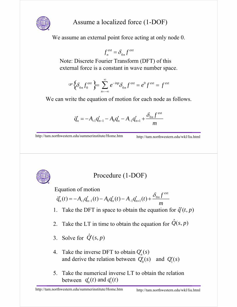
Assume a localized force (1-DOF)
We assume an external point force acting at only node 0.
We can write the equation of motion for each node as follows.
ext0
1 1 0 1 1n
n n n n
fq A q A q A q
m
δ+ − − +′ ′ ′ ′= − − − +&&
fnext = δ
0nf ext
Note: Discrete Fourier Transform (DFT) of this external force is a constant in wave number space.
δ
0nf
0ext = e− inpδ
0nf ext
n=−∞
∞
∑ = e0 f ext = f ext
http://tam.northwestern.edu/summerinstitute/Home.htm http://tam.northwestern.edu/wkl/liu.html
Procedure (1-DOF)
1. Take the DFT in space to obtain the equation for
2. Take the LT in time to obtain the equation for
3. Solve for
4. Take the inverse DFT to obtainand derive the relation between and
5. Take the numerical inverse LT to obtain the relationbetween
ext0
1 1 0 1 1( ) ( ) ( ) ( ) nn n n n
fq t A q t A q t A q t
m
δ+ − − +′ ′ ′ ′= − − − +&&
ˆ ( , )q t p′
ˆ ( , )Q s p
ˆ ( , )Q s p′
′Qn(s)
′Q0(s) ′Q
1(s)
′q0(t) and ′q
1(t)
Equation of motion
http://tam.northwestern.edu/summerinstitute/Home.htm http://tam.northwestern.edu/wkl/liu.html
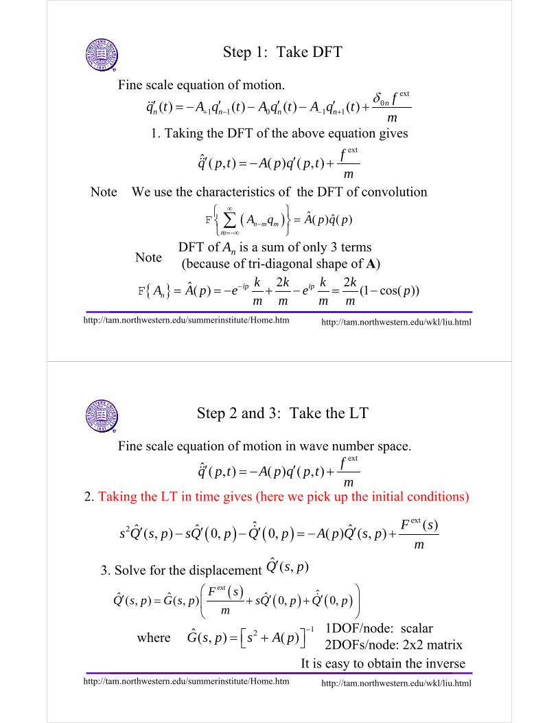
Step 1: Take DFT
ext
ˆ ( , ) ( ) ( , )f
q p t A p q p tm
′ ′= − +&&
1. Taking the DFT of the above equation gives
2 2ˆ( ) (1 cos( ))ip ipn
k k k kA A p e e p
m m m m−= = − + − = −F
DFT of An is a sum of only 3 terms(because of tri-diagonal shape of A)
Note
ext0
1 1 0 1 1( ) ( ) ( ) ( ) nn n n n
fq t A q t A q t A q t
m
δ+ − − +′ ′ ′ ′= − − − +&&
( ) ˆ ˆ( ) ( )n m mm
A q A p q p∞
−=−∞
⎧ ⎫=⎨ ⎬
⎩ ⎭∑F
We use the characteristics of the DFT of convolution
Note
Fine scale equation of motion.
http://tam.northwestern.edu/summerinstitute/Home.htm http://tam.northwestern.edu/wkl/liu.html
Step 2 and 3: Take the LT
( ) ( )ext
2 ( )ˆˆ ˆ ˆ( , ) 0, 0, ( ) ( , )F s
s Q s p sQ p Q p A p Q s pm
′ ′ ′ ′− − = − +&
( ) ( ) ( )ˆˆ ˆ ˆ( , ) ( , ) 0, 0,extF s
Q s p G s p sQ p Q pm
⎛ ⎞′ ′ ′= + +⎜ ⎟
⎝ ⎠&
12ˆ ( , ) ( )G s p s A p−
⎡ ⎤= +⎣ ⎦It is easy to obtain the inverse
2. Taking the LT in time gives (here we pick up the initial conditions)
3. Solve for the displacement
1DOF/node: scalar2DOFs/node: 2x2 matrix
ˆ ( , )Q s p′
where
ext
ˆ ( , ) ( ) ( , )f
q p t A p q p tm
′ ′= − +&&
Fine scale equation of motion in wave number space.
http://tam.northwestern.edu/summerinstitute/Home.htm http://tam.northwestern.edu/wkl/liu.html
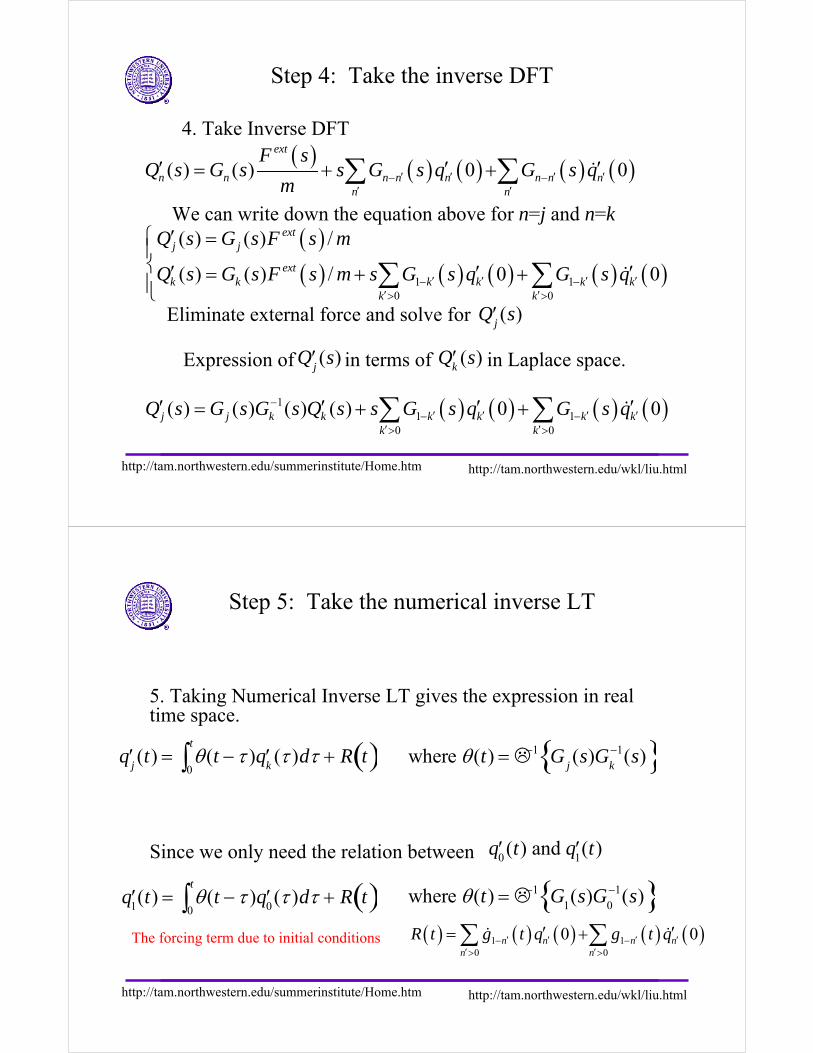
Step 4: Take the inverse DFT
( ) ( ) ( ) ( )11 1
0 0
( ) ( ) ( ) ( ) 0 0j j k k k k k kk k
Q s G s G s Q s s G s q G s q−′ ′ ′ ′− −
′ ′> >
′ ′ ′ ′= + +∑ ∑ &
( ) ( ) ( ) ( ) ( )( ) ( ) 0 0ext
n n n n n n n nn n
F sQ s G s s G s q G s q
m′ ′ ′ ′− −
′ ′
′ ′ ′= + +∑ ∑ &
4. Take Inverse DFT
We can write down the equation above for n=j and n=k( )( ) ( ) ( ) ( ) ( )1 1
0 0
( ) ( ) /
( ) ( ) / 0 0
extj j
extk k k k k k
k k
Q s G s F s m
Q s G s F s m s G s q G s q′ ′ ′ ′− −′ ′> >
′⎧ =⎪⎨ ′ ′ ′= + +⎪⎩
∑ ∑ &
Eliminate external force and solve for ′Qj(s)
Expression of in terms of in Laplace space. ′Qj(s) ′Q
k(s)
http://tam.northwestern.edu/summerinstitute/Home.htm http://tam.northwestern.edu/wkl/liu.html
Step 5: Take the numerical inverse LT
′qj(t) = θ(t − τ ) ′q
k(τ )dτ
0
t
∫ + R t( )
5. Taking Numerical Inverse LT gives the expression in real time space.
where θ(t) = −1 G
j(s)G
k−1(s)
Since we only need the relation between ′q0(t) and ′q
1(t)
′q1(t) = θ(t − τ ) ′q
0(τ )dτ
0
t
∫ + R t( ) where θ(t) = −1 G
1(s)G
0−1(s)
( ) ( ) ( ) ( ) ( )1 10 0
0 0n n n nn n
R t g t q g t q′ ′ ′ ′− −′ ′> >
′ ′= +∑ ∑& &The forcing term due to initial conditions
http://tam.northwestern.edu/summerinstitute/Home.htm http://tam.northwestern.edu/wkl/liu.html
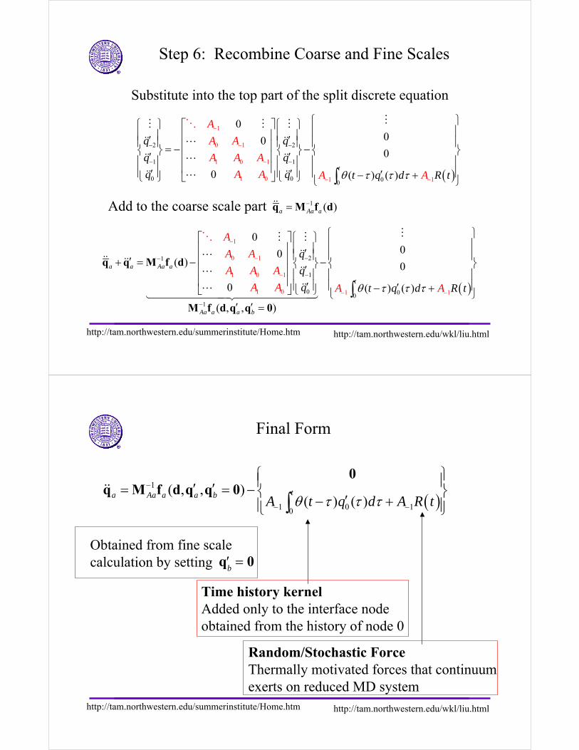
Step 6: Recombine Coarse and Fine Scales
Substitute into the top part of the split discrete equation
( )
1
0 1
1
2 2
1 1
0 0 00
0 1
1 0 1 1
0000
0 ( ) ( )t
q q
q q
q
A
A A
A A A
A A A Aq t q d R tθ τ τ τ
−
−− −
− −−
− −
⎧ ⎫⎧ ⎫ ⎡ ⎤ ⎧ ⎫⎪ ⎪⎪ ⎪ ⎢ ⎥ ⎪ ⎪′ ′⎪ ⎪ ⎪ ⎪ ⎪ ⎪⎢ ⎥= − −⎨ ⎬ ⎨ ⎬ ⎨ ⎬′ ′⎢ ⎥⎪ ⎪ ⎪ ⎪ ⎪ ⎪⎢ ⎥⎪ ⎪ ⎪ ⎪ ⎪ ⎪′ ′ ′− +⎩ ⎭ ⎣ ⎦ ⎩ ⎭ ⎩ ⎭∫
MM M M
&& &&L
&& &&L
&
O
&& &L
Add to the coarse scale part
( )
1
0 1
1 0 1
1
21
1
0 0010
1
1
000
( ) 0
0 ( ) ( )
( , , )
q q M f d
M f d q q 0
a a Aa a
t
Aa a a b
A
A A
A A A
q
q
q t qA tA A Ad Rθ τ τ τ
−
−
−
− −
−−
−
−
⎧ ⎫⎡ ⎤ ⎧ ⎫⎪ ⎪⎢ ⎥ ⎪ ⎪′⎪ ⎪ ⎪ ⎪⎢ ⎥′+ = − −⎨ ⎬ ⎨ ⎬′⎢ ⎥ ⎪ ⎪ ⎪ ⎪⎢ ⎥ ⎪ ⎪ ⎪ ⎪′ ′− +⎣ ⎦ ⎩ ⎭ ⎩ ⎭
′ ′ =∫
MM M
&&L&& &&&&L
&&L14444444244444443
O
1 ( )q M f da Aa a−=&&
http://tam.northwestern.edu/summerinstitute/Home.htm http://tam.northwestern.edu/wkl/liu.html
Final Form
( )1
1 0 10
( , , )( ) ( )
0q M f d q q 0 ta Aa a a b
A t q d A R tθ τ τ τ−
− −
⎧ ⎫⎪ ⎪′ ′= = − ⎨ ⎬′− +⎪ ⎪⎩ ⎭∫&&
Time history kernelAdded only to the interface nodeobtained from the history of node 0
Obtained from fine scalecalculation by setting ′q
b= 0
Random/Stochastic ForceThermally motivated forces that continuum exerts on reduced MD system
http://tam.northwestern.edu/summerinstitute/Home.htm http://tam.northwestern.edu/wkl/liu.html
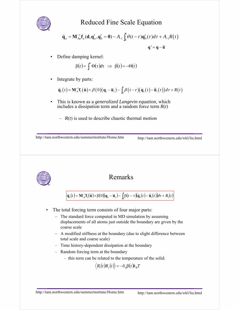
Reduced Fine Scale Equation
• Define damping kernel:
• Integrate by parts:
• This is known as a generalized Langevin equation, which includes a dissipation term and a random force term R(t)
– R(t) is used to describe chaotic thermal motion
( )11 0 10
( , , ) ( ) ( )q M f d q q 0 qt
a Aa a a b A t d A R tθ τ τ τ−− −′ ′ ′= = − − +∫&&
( ) ( ) ( )( ) ( ) ( ) ( )( ) ( )11 1 1 1 1 10
0q M f u q u q ut
At t t t d R tβ β τ τ−= + − − − − +∫ &&& &%
( ) ( ) ( ) ( )ttdtt
Θ−=β⇒ττΘ=β ∫∞ &
'q q u= −
http://tam.northwestern.edu/summerinstitute/Home.htm http://tam.northwestern.edu/wkl/liu.html
Remarks
• The total forcing term consists of four major parts:– The standard force computed in MD simulation by assuming
displacements of all atoms just outside the boundary are given by the coarse scale
– A modified stiffness at the boundary (due to slight difference between total scale and coarse scale)
– Time history-dependent dissipation at the boundary
– Random forcing term at the boundary
– this term can be related to the temperature of the solid:
( ) ( ) ( )( ) ( ) ( ) ( )( ) ( )tRdttttt
A 10 111111
1 0~ +τ−τ−β−−β+= ∫− uququfMq &&&&
( ) ( ) ( ) TkttRtR Bijji βδ−=
http://tam.northwestern.edu/summerinstitute/Home.htm http://tam.northwestern.edu/wkl/liu.html
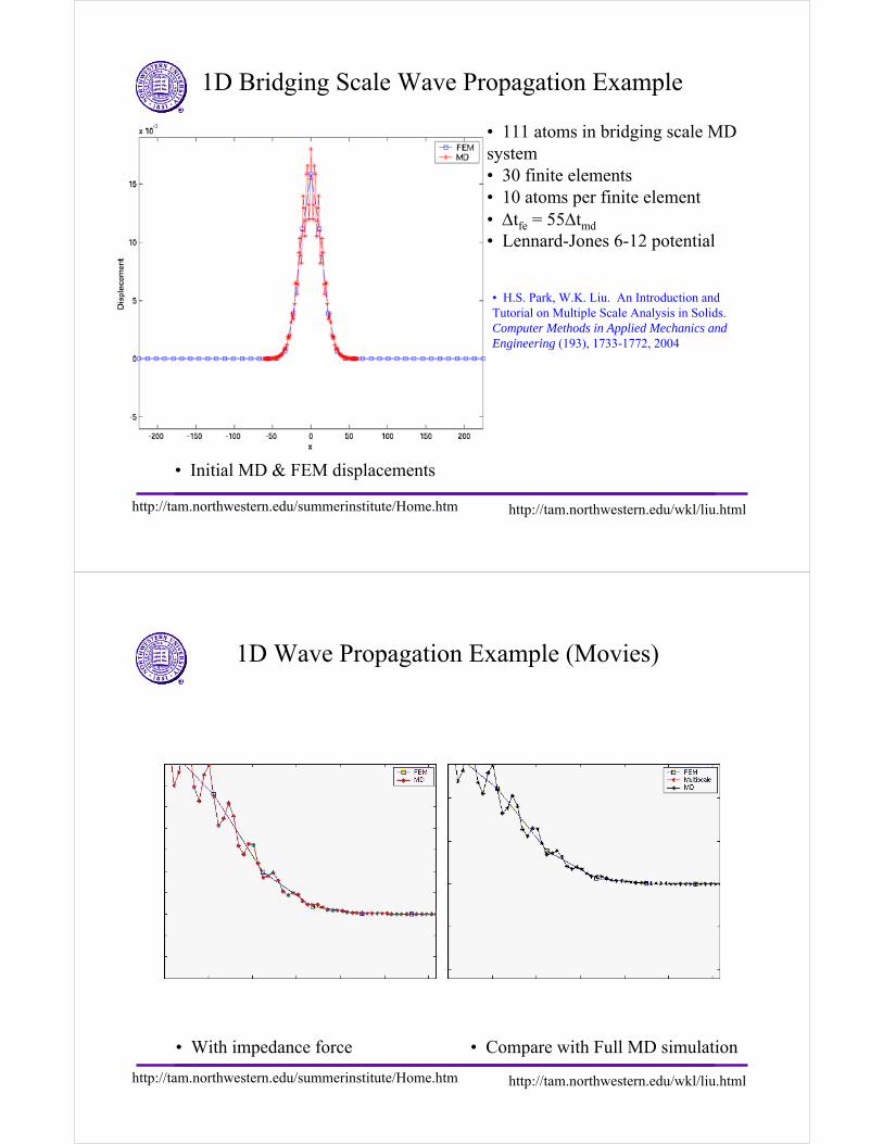
1D Bridging Scale Wave Propagation Example
• 111 atoms in bridging scale MD system• 30 finite elements• 10 atoms per finite element• ∆tfe = 55∆tmd
• Lennard-Jones 6-12 potential
• Initial MD & FEM displacements
• H.S. Park, W.K. Liu. An Introduction and Tutorial on Multiple Scale Analysis in Solids. Computer Methods in Applied Mechanics and Engineering (193), 1733-1772, 2004
http://tam.northwestern.edu/summerinstitute/Home.htm http://tam.northwestern.edu/wkl/liu.html
1D Wave Propagation Example (Movies)
• Compare with Full MD simulation• With impedance force
http://tam.northwestern.edu/summerinstitute/Home.htm http://tam.northwestern.edu/wkl/liu.html
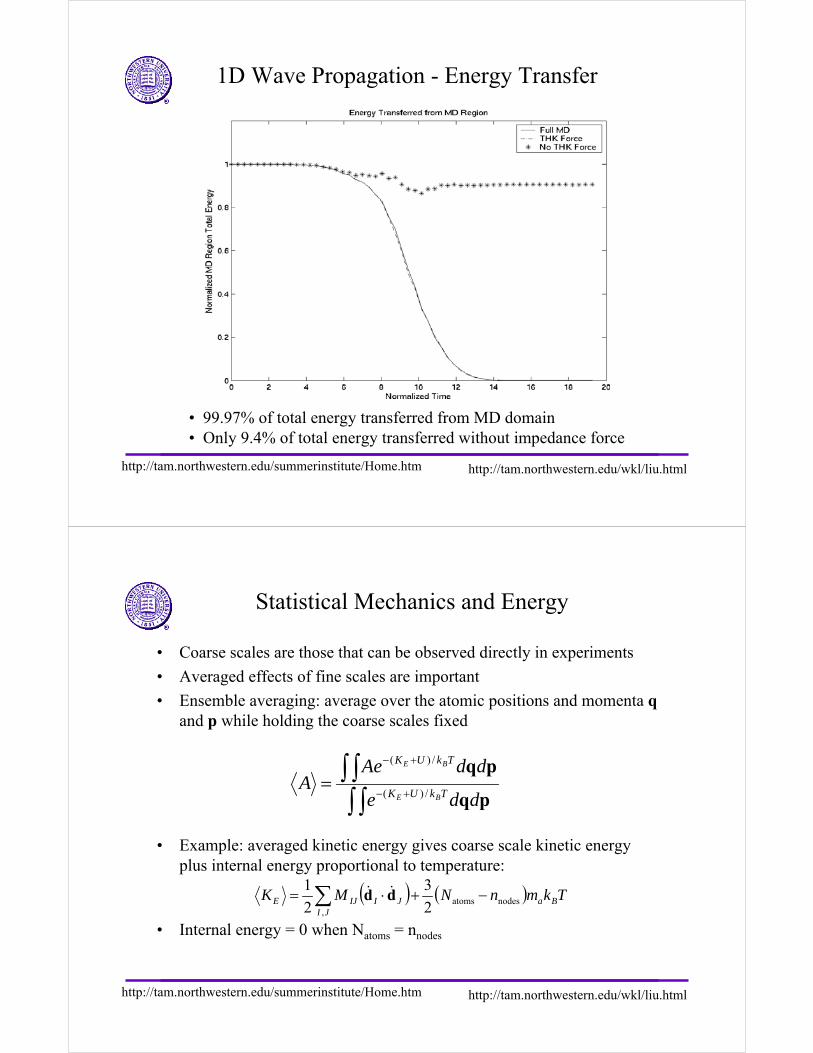
1D Wave Propagation - Energy Transfer
• 99.97% of total energy transferred from MD domain• Only 9.4% of total energy transferred without impedance force
http://tam.northwestern.edu/summerinstitute/Home.htm http://tam.northwestern.edu/wkl/liu.html
Statistical Mechanics and Energy
• Coarse scales are those that can be observed directly in experiments
• Averaged effects of fine scales are important
• Ensemble averaging: average over the atomic positions and momenta qand p while holding the coarse scales fixed
• Example: averaged kinetic energy gives coarse scale kinetic energy plus internal energy proportional to temperature:
• Internal energy = 0 when Natoms = nnodes
∫ ∫∫ ∫
+−
+−
=pq
pq
dde
ddAeA
TkUK
TkUK
BE
BE
/)(
/)(
( ) ( ) TkmnNMK BaJI
JIIJE nodesatoms, 2
3
2
1−+⋅= ∑ dd &&
http://tam.northwestern.edu/summerinstitute/Home.htm http://tam.northwestern.edu/wkl/liu.html
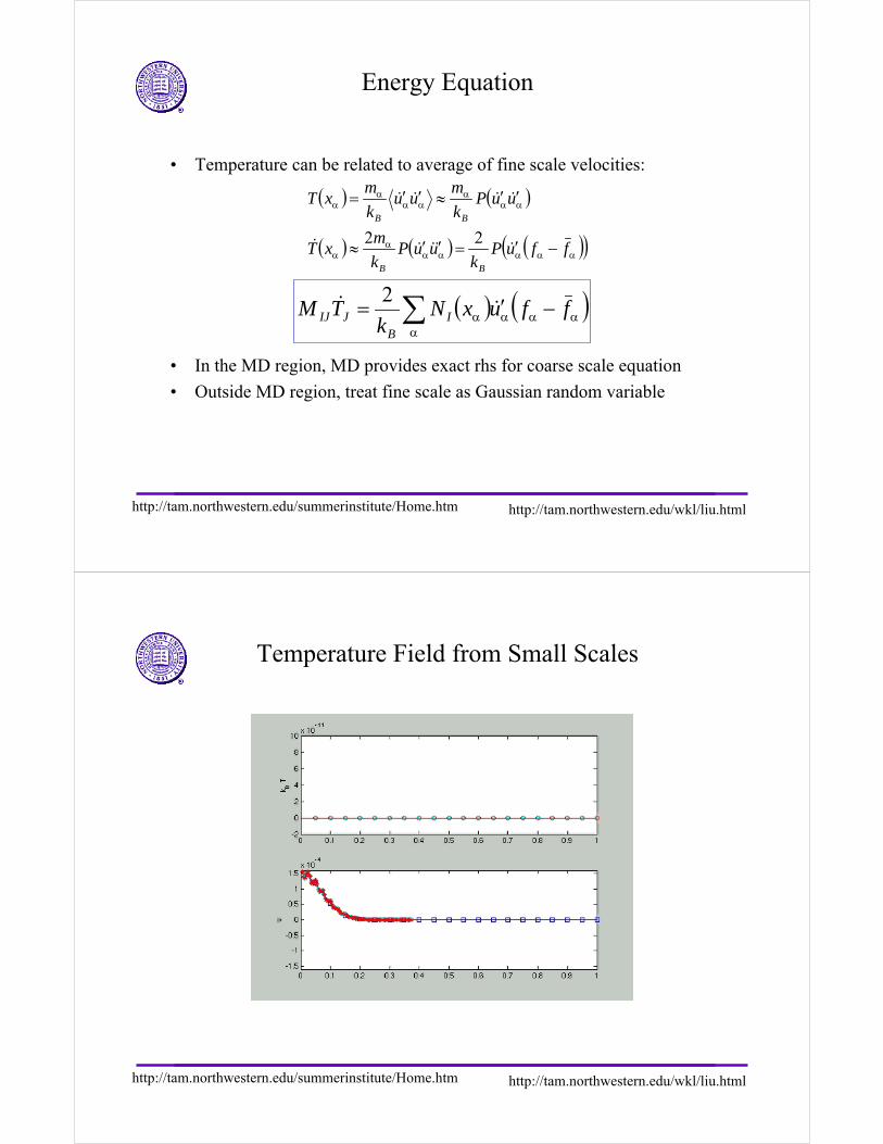
Energy Equation
• Temperature can be related to average of fine scale velocities:
• In the MD region, MD provides exact rhs for coarse scale equation
• Outside MD region, treat fine scale as Gaussian random variable
( ) ( )
( ) ( ) ( )( )αααααα
α
ααα
ααα
α
−′=′′≈
′′≈′′=
ffuPk
uuPk
mxT
uuPk
muu
k
mxT
BB
BB
&&&&&
&&&&
22
( ) ( )∑α
αααα −′= ffuxNk
TM IB
JIJ && 2
http://tam.northwestern.edu/summerinstitute/Home.htm http://tam.northwestern.edu/wkl/liu.html
Temperature Field from Small Scales
http://tam.northwestern.edu/summerinstitute/Home.htm http://tam.northwestern.edu/wkl/liu.html
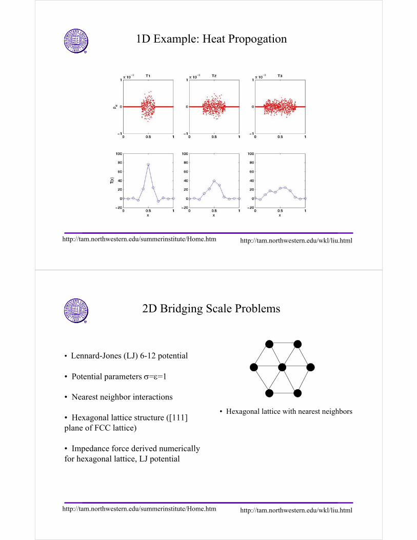
1D Example: Heat Propogation
http://tam.northwestern.edu/summerinstitute/Home.htm http://tam.northwestern.edu/wkl/liu.html
2D Bridging Scale Problems
• Lennard-Jones (LJ) 6-12 potential
• Potential parameters σ=ε=1
• Nearest neighbor interactions
• Hexagonal lattice structure ([111] plane of FCC lattice)
• Impedance force derived numericallyfor hexagonal lattice, LJ potential
• Hexagonal lattice with nearest neighbors
http://tam.northwestern.edu/summerinstitute/Home.htm http://tam.northwestern.edu/wkl/liu.html
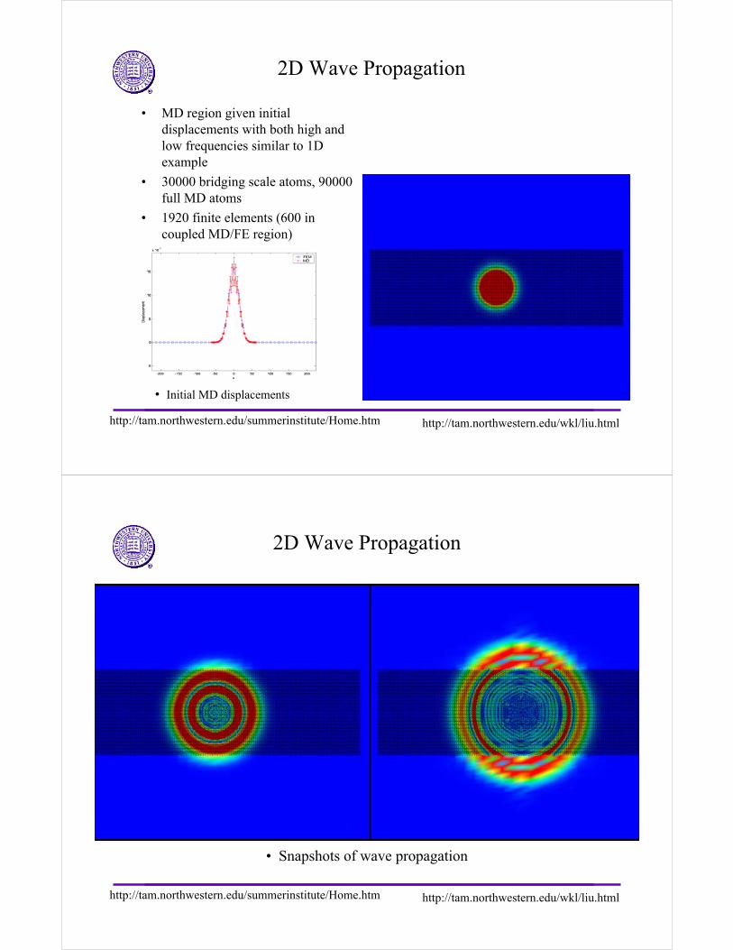
2D Wave Propagation
• MD region given initial displacements with both high and low frequencies similar to 1D example
• 30000 bridging scale atoms, 90000 full MD atoms
• 1920 finite elements (600 in coupled MD/FE region)
• 50 atoms per finite element
• Initial MD displacements
http://tam.northwestern.edu/summerinstitute/Home.htm http://tam.northwestern.edu/wkl/liu.html
2D Wave Propagation
• Snapshots of wave propagation
http://tam.northwestern.edu/summerinstitute/Home.htm http://tam.northwestern.edu/wkl/liu.html
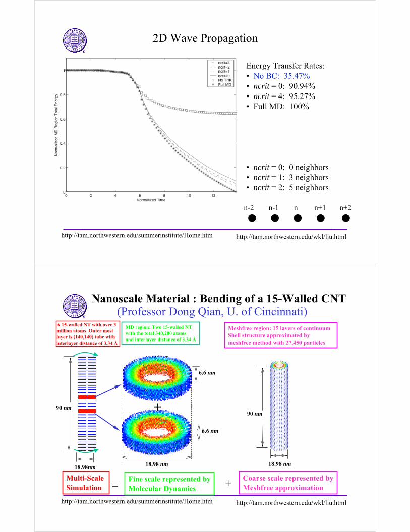
2D Wave Propagation
Energy Transfer Rates:• No BC: 35.47%• ncrit = 0: 90.94%• ncrit = 4: 95.27%• Full MD: 100%
• ncrit = 0: 0 neighbors• ncrit = 1: 3 neighbors• ncrit = 2: 5 neighbors
n n+1 n+2n-1n-2
http://tam.northwestern.edu/summerinstitute/Home.htm http://tam.northwestern.edu/wkl/liu.html
A 15-walled NT with over 3 million atoms. Outer most layer is (140,140) tube with interlayer distance of 3.34 Å
=Multi-ScaleSimulation
90 nm
18.98nm
MD region: Two 15-walled NT with the total 340,200 atomsand interlayer distance of 3.34 Å
+
Fine scale represented byMolecular Dynamics
6.6 nm
6.6 nm
18.98 nm
Meshfree region: 15 layers of continuumShell structure approximated by meshfree method with 27,450 particles
Coarse scale represented byMeshfree approximation+
18.98 nm
90 nm
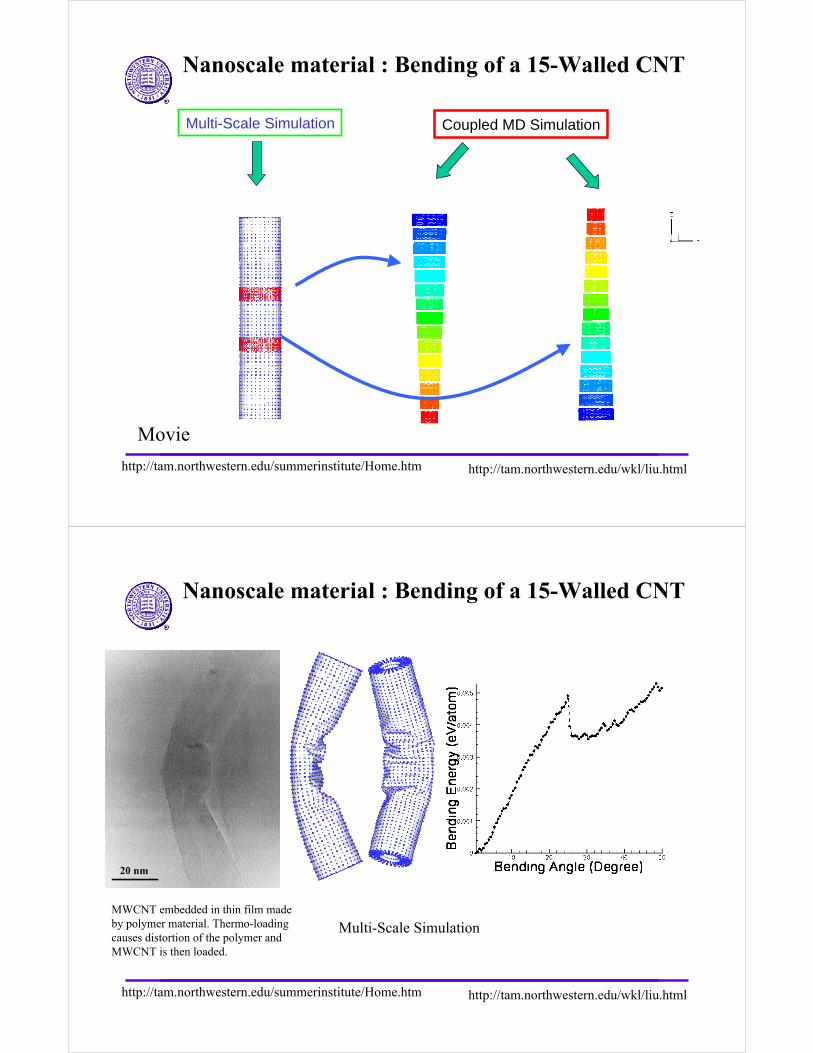
Nanoscale Material : Bending of a 15-Walled CNT(Professor Dong Qian, U. of Cincinnati)
http://tam.northwestern.edu/summerinstitute/Home.htm http://tam.northwestern.edu/wkl/liu.html
Multi-Scale Simulation Coupled MD Simulation
Nanoscale material : Bending of a 15-Walled CNT
Movie
http://tam.northwestern.edu/summerinstitute/Home.htm http://tam.northwestern.edu/wkl/liu.html
MWCNT embedded in thin film made by polymer material. Thermo-loading causes distortion of the polymer and MWCNT is then loaded.
Multi-Scale Simulation
Nanoscale material : Bending of a 15-Walled CNT

http://tam.northwestern.edu/summerinstitute/Home.htm http://tam.northwestern.edu/wkl/liu.html
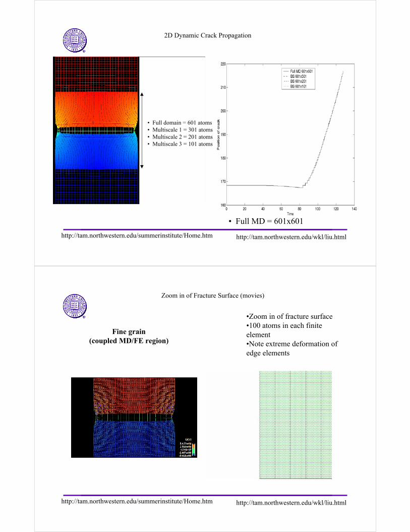
Example : 2D Dynamic Crack Propagation
Problem Description:• LJ 6-12 potential• Nearest neighbor interactions• 90000 atoms, 1800 finite elements (900 in coupled region)• 100 atoms per finite element• 40 MD time steps per FEM time step• Ramp velocity BC on FEM• Full MD = 180,000 atoms
• H.S. Park, E.G. Karpov, P.A. Klein and W.K. Liu, The Bridging Scale for Two-Dimensional Atomistic/Continuum Coupling, submitted to Philosophical Magazine A, 2003
http://tam.northwestern.edu/summerinstitute/Home.htm http://tam.northwestern.edu/wkl/liu.html
2D Dynamic Crack Propagation (movies)
Entire domain for coupled crackpropagation example
results
Ref: Harold Park
Finite elements
MD domain
http://tam.northwestern.edu/summerinstitute/Home.htm http://tam.northwestern.edu/wkl/liu.html
2D Dynamic Crack Propagation
• Full MD = 601x601
• Full domain = 601 atoms• Multiscale 1 = 301 atoms • Multiscale 2 = 201 atoms• Multiscale 3 = 101 atoms
http://tam.northwestern.edu/summerinstitute/Home.htm http://tam.northwestern.edu/wkl/liu.html
Zoom in of Fracture Surface (movies)
•Zoom in of fracture surface •100 atoms in each finite element•Note extreme deformation of edge elements
Fine grain(coupled MD/FE region)
http://tam.northwestern.edu/summerinstitute/Home.htm http://tam.northwestern.edu/wkl/liu.html
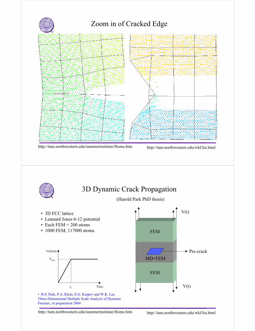
Zoom in of Cracked Edge
http://tam.northwestern.edu/summerinstitute/Home.htm http://tam.northwestern.edu/wkl/liu.html
3D Dynamic Crack Propagation
• 3D FCC lattice• Lennard Jones 6-12 potential• Each FEM = 200 atoms• 1000 FEM, 117000 atoms
Time
Velocity
t1
Vmax
FEM
FEM
MD+FEM
Pre-crack
V(t)
V(t)
• H.S. Park, P.A. Klein, E.G. Karpov and W.K. Liu, Three-Dimensional Multiple Scale Analysis of DynamicFracture, in preparation 2004
(Harold Park PhD thesis)
http://tam.northwestern.edu/summerinstitute/Home.htm http://tam.northwestern.edu/wkl/liu.html
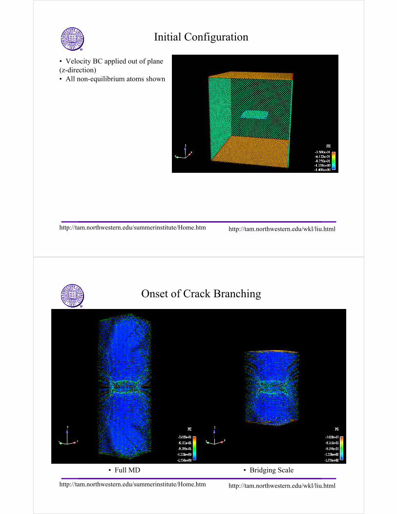
Initial Configuration
• Velocity BC applied out of plane(z-direction)• All non-equilibrium atoms shown
http://tam.northwestern.edu/summerinstitute/Home.htm http://tam.northwestern.edu/wkl/liu.html
Onset of Crack Branching
• Full MD • Bridging Scale
http://tam.northwestern.edu/summerinstitute/Home.htm http://tam.northwestern.edu/wkl/liu.html
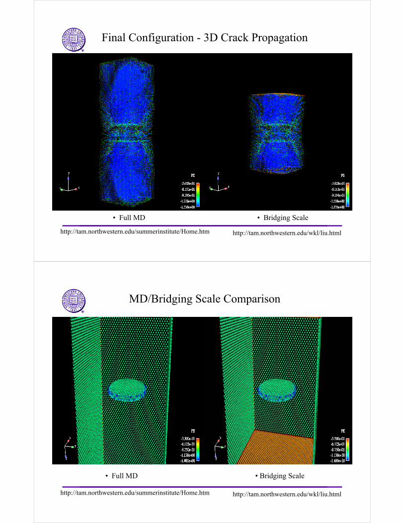
Final Configuration - 3D Crack Propagation
• Full MD • Bridging Scale
http://tam.northwestern.edu/summerinstitute/Home.htm http://tam.northwestern.edu/wkl/liu.html
MD/Bridging Scale Comparison
• Full MD • Bridging Scale
http://tam.northwestern.edu/summerinstitute/Home.htm http://tam.northwestern.edu/wkl/liu.html
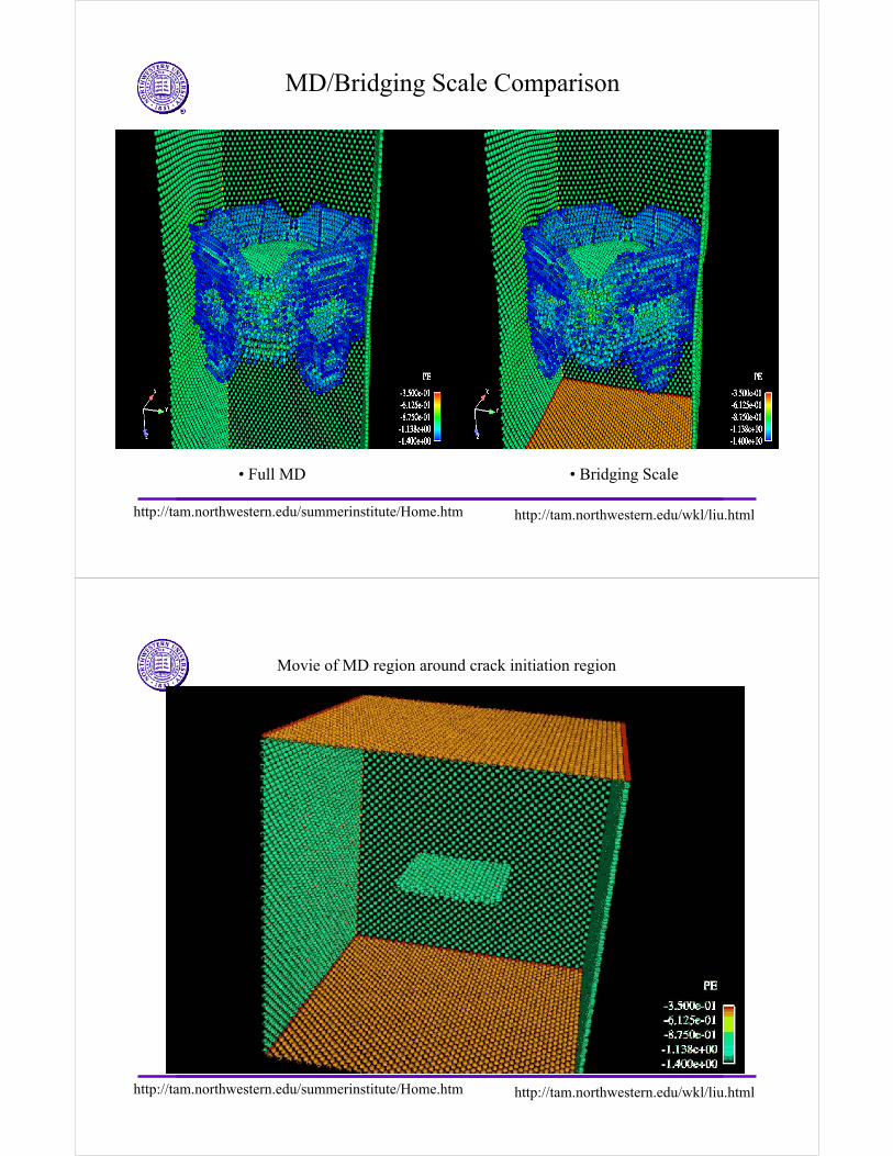
MD/Bridging Scale Comparison
• Full MD • Bridging Scale
http://tam.northwestern.edu/summerinstitute/Home.htm http://tam.northwestern.edu/wkl/liu.html
Movie of MD region around crack initiation region
http://tam.northwestern.edu/summerinstitute/Home.htm http://tam.northwestern.edu/wkl/liu.html
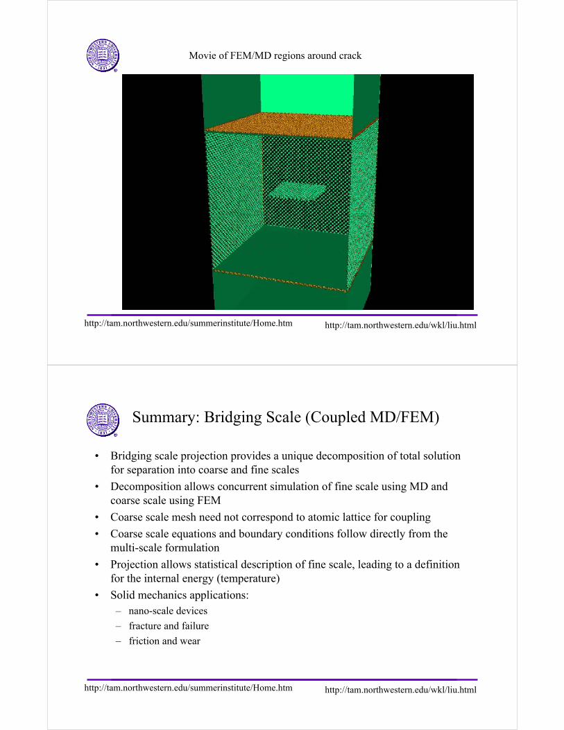
Movie of FEM/MD regions around crack
http://tam.northwestern.edu/summerinstitute/Home.htm http://tam.northwestern.edu/wkl/liu.html
Summary: Bridging Scale (Coupled MD/FEM)
• Bridging scale projection provides a unique decomposition of total solution for separation into coarse and fine scales
• Decomposition allows concurrent simulation of fine scale using MD and coarse scale using FEM
• Coarse scale mesh need not correspond to atomic lattice for coupling
• Coarse scale equations and boundary conditions follow directly from the multi-scale formulation
• Projection allows statistical description of fine scale, leading to a definition for the internal energy (temperature)
• Solid mechanics applications:– nano-scale devices
– fracture and failure
– friction and wear
http://tam.northwestern.edu/summerinstitute/Home.htm http://tam.northwestern.edu/wkl/liu.html
• Self Study Materials
http://tam.northwestern.edu/summerinstitute/Home.htm http://tam.northwestern.edu/wkl/liu.html
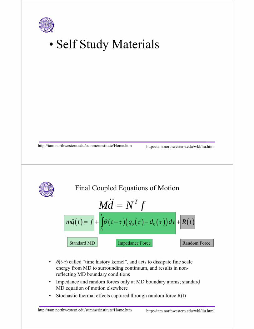
Final Coupled Equations of Motion
• θ(t-τ) called “time history kernel”, and acts to dissipate fine scale energy from MD to surrounding continuum, and results in non-reflecting MD boundary conditions
• Impedance and random forces only at MD boundary atoms; standard MD equation of motion elsewhere
• Stochastic thermal effects captured through random force R(t)
TMd N f=&&
( ) ( ) ( ) ( )( ) ( )0 0
0
t
mq t f t q d d R tθ τ τ τ τ= + − − +∫&&
Standard MD Impedance Force Random Force
http://tam.northwestern.edu/summerinstitute/Home.htm http://tam.northwestern.edu/wkl/liu.html
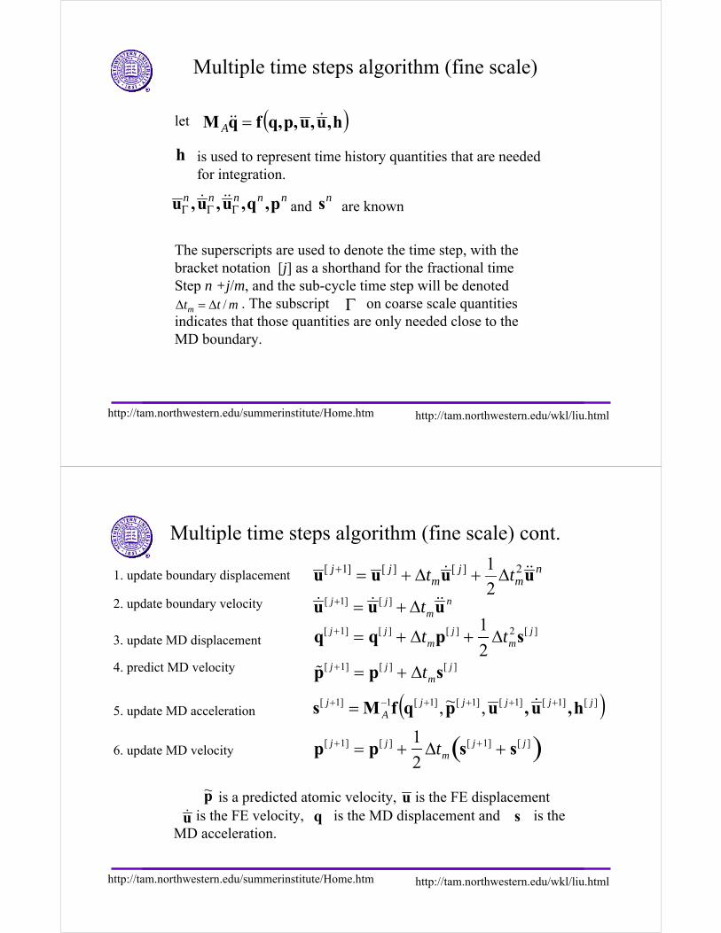
is used to represent time history quantities that are needed for integration.
let ( )h,u,up,q,fqM &&& =A
h
nnnnn p,q,u,u,u ΓΓΓ&&& nsand are known
Γ
The superscripts are used to denote the time step, with the bracket notation [j] as a shorthand for the fractional timeStep n +j/m, and the sub-cycle time step will be denoted
. The subscript on coarse scale quantitiesindicates that those quantities are only needed close to the MD boundary.
mttm /∆=∆
Multiple time steps algorithm (fine scale)
http://tam.northwestern.edu/summerinstitute/Home.htm http://tam.northwestern.edu/wkl/liu.html
nm
jm
jj tt uuuu &&& 2][][]1[
2
1∆+∆+=+
nm
jj t uuu &&&& ∆+=+ ][]1[
q[ j +1] = q[ j ] + ∆tmp[ j ] +1
2∆tm
2 s[ j ]
%p[ j +1] = p[ j ] + ∆tms[ j ]
( )][]1[]1[]1[]1[1]1[ ,~, jjjjjA
j h,u,upqfMs ++++−+ = &
p[ j +1] = p[ j ] +1
2∆tm s[ j +1] + s[ j ]( )
is a predicted atomic velocity, is the FE displacementis the FE velocity, is the MD displacement and is the
MD acceleration.
p~ uu& q s
Multiple time steps algorithm (fine scale) cont.
1. update boundary displacement
2. update boundary velocity
3. update MD displacement
4. predict MD velocity
5. update MD acceleration
6. update MD velocity
http://tam.northwestern.edu/summerinstitute/Home.htm http://tam.northwestern.edu/wkl/liu.html
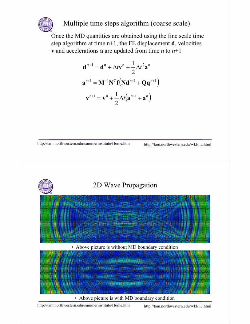
nnnn tt avdd 21
2
1∆+∆+=+
( )1111 ++−+ += nnTn QqNdfNMa
( )nnnn t aavv +∆+= ++ 11
2
1
Once the MD quantities are obtained using the fine scale time step algorithm at time n+1, the FE displacement d, velocitiesv and accelerations a are updated from time n to n+1
Multiple time steps algorithm (coarse scale)
http://tam.northwestern.edu/summerinstitute/Home.htm http://tam.northwestern.edu/wkl/liu.html
2D Wave Propagation
• Above picture is without MD boundary condition
• Above picture is with MD boundary condition
http://tam.northwestern.edu/summerinstitute/Home.htm http://tam.northwestern.edu/wkl/liu.html
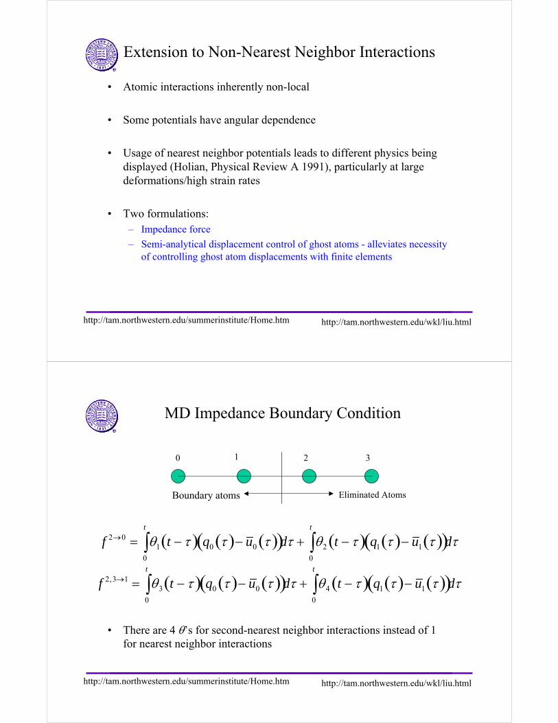
Extension to Non-Nearest Neighbor Interactions
• Atomic interactions inherently non-local
• Some potentials have angular dependence
• Usage of nearest neighbor potentials leads to different physics being displayed (Holian, Physical Review A 1991), particularly at large deformations/high strain rates
• Two formulations:– Impedance force
– Semi-analytical displacement control of ghost atoms - alleviates necessity of controlling ghost atom displacements with finite elements
http://tam.northwestern.edu/summerinstitute/Home.htm http://tam.northwestern.edu/wkl/liu.html
MD Impedance Boundary Condition
• There are 4 θ’s for second-nearest neighbor interactions instead of 1 for nearest neighbor interactions
f 2→0 = θ1 t − τ( ) q0 τ( )− u0 τ( )( )0
t
∫ dτ + θ2 t − τ( ) q1 τ( )− u1 τ( )( )0
t
∫ dτ
f 2,3→1 = θ3 t − τ( ) q0 τ( )− u0 τ( )( )0
t
∫ dτ + θ4 t − τ( ) q1 τ( )− u1 τ( )( )0
t
∫ dτ
0 1 2 3
Eliminated AtomsBoundary atoms
http://tam.northwestern.edu/summerinstitute/Home.htm http://tam.northwestern.edu/wkl/liu.html
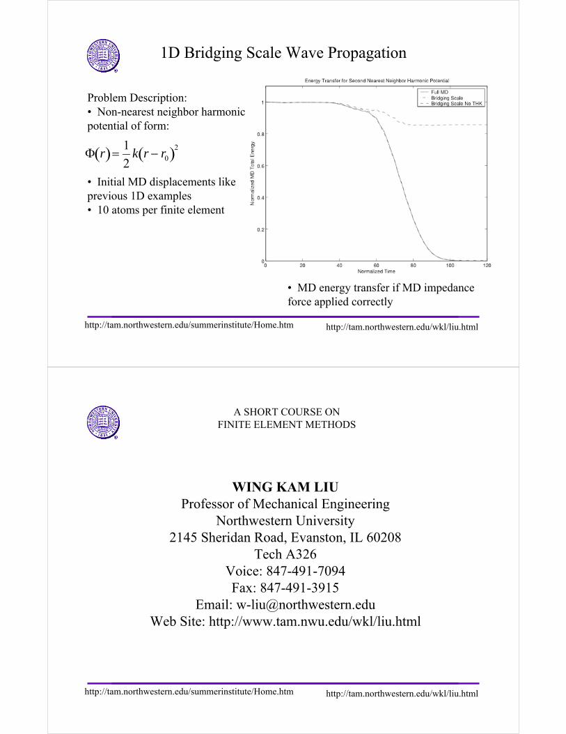
1D Bridging Scale Wave Propagation
Problem Description:• Non-nearest neighbor harmonic potential of form:
• Initial MD displacements like previous 1D examples• 10 atoms per finite element
• MD energy transfer if MD impedance force applied correctly
Φ r( )=1
2k r − r0( )2
http://tam.northwestern.edu/summerinstitute/Home.htm http://tam.northwestern.edu/wkl/liu.html
A SHORT COURSE ONFINITE ELEMENT METHODS
WING KAM LIUProfessor of Mechanical Engineering
Northwestern University2145 Sheridan Road, Evanston, IL 60208
Tech A326Voice: 847-491-7094Fax: 847-491-3915
Email: [email protected] Site: http://www.tam.nwu.edu/wkl/liu.html
http://tam.northwestern.edu/summerinstitute/Home.htm http://tam.northwestern.edu/wkl/liu.html
References
• S.P.Timoshenko, “Theory of Elasticity”, 3rd edition, McGraw-Hill Publishing Company, 1987
• T.J.R.Hughes, “The Finite Element Method”, Prentice-Hall International Inc., 1987
• O.C.Zienkiewicz and R.L.Taylor, “The Finite Element Method”, 4th edition, Vol.1,McGraw-Hill International Editions, 1989
• R.D.Cook, D.S.Malkus and M.E.Plesha, “Concepts and Applications of Finite Element Analysis”, 3rd edition, John Wiley & Sons, 1989
• R.H.Gallagher, “Finite Element Analysis: Fundamentals”, Prentice-Hall Inc.,1975
•T. Belytschko, W. K. Liu and B. Moran, “Nonlinear Finite Elements for Continua and Structures”, John Wiley and Sons, 2000.
http://tam.northwestern.edu/summerinstitute/Home.htm http://tam.northwestern.edu/wkl/liu.html
OUTLINE
Section I. Nature of Finite Element Method
Section II. 1-D Linear Elasticity
Section III. 1-D Nonlinear Elasticity
Section IV. Hamiltonian in Molecular Dynamics and
Comparison of FEM with MD
http://tam.northwestern.edu/summerinstitute/Home.htm http://tam.northwestern.edu/wkl/liu.html
Section 1
NATURE OF F.E.M.
Step 1: Discretion of a continuous system
Step 2: Determination of finite element matrices from the
geometry, material, and loading data
Step 3: Assembly of the finite element matrices
Step 4: Displacement and traction boundry conditions
Step 5: Solve the resulting equation system and interpretation of
the results (post-processing)
http://tam.northwestern.edu/summerinstitute/Home.htm http://tam.northwestern.edu/wkl/liu.html
Type of Elements
http://tam.northwestern.edu/summerinstitute/Home.htm http://tam.northwestern.edu/wkl/liu.html
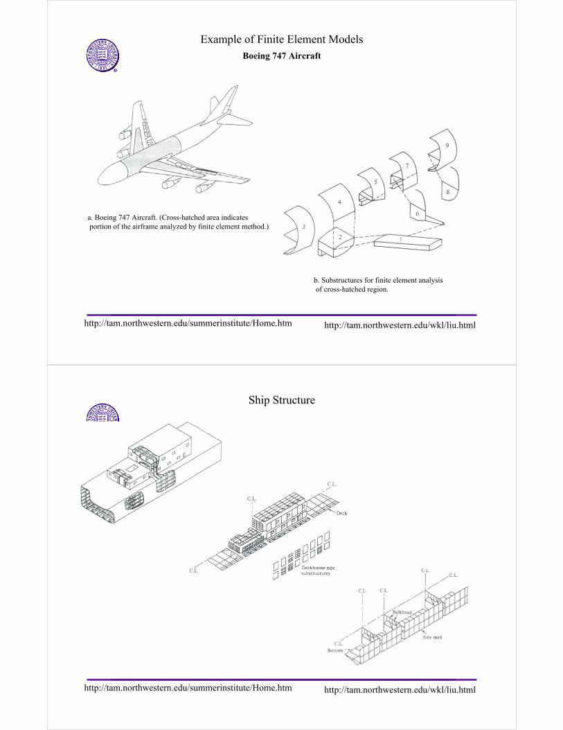
Example of Finite Element ModelsBoeing 747 Aircraft
a. Boeing 747 Aircraft. (Cross-hatched area indicatesportion of the airframe analyzed by finite element method.)
b. Substructures for finite element analysisof cross-hatched region.
http://tam.northwestern.edu/summerinstitute/Home.htm http://tam.northwestern.edu/wkl/liu.html
Ship Structure
http://tam.northwestern.edu/summerinstitute/Home.htm http://tam.northwestern.edu/wkl/liu.html
Section II
LINEAR ELASTICITY IN 1-D
• Matrix Method
1) Stiffness matrix
2) Assembly
• Finite Element Method
1) Governing equations
2) Strong form and weak form
3) Principle of virtual work
4) Finite element approximation
http://tam.northwestern.edu/summerinstitute/Home.htm http://tam.northwestern.edu/wkl/liu.html
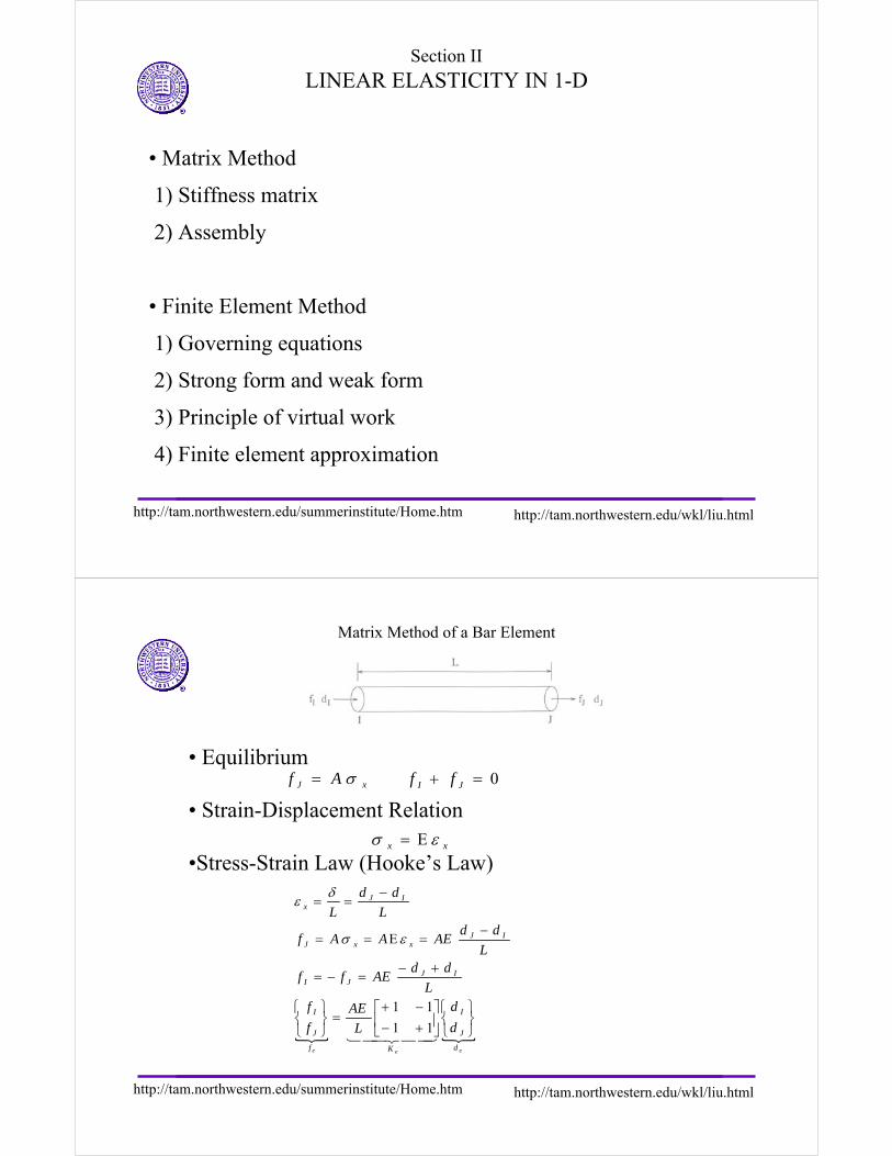
Matrix Method of a Bar Element
• Equilibrium
• Strain-Displacement Relation
•Stress-Strain Law (Hooke’s Law)
xJ Af σ= 0=+ JI ff
xx εσ Ε=
eee d
J
I
Kf
J
I
IJJI
IJxxJ
IJx
d
d
L
AE
f
fL
ddAEff
L
ddAEAAf
L
dd
L
⎭⎬⎫
⎩⎨⎧
⎥⎦
⎤⎢⎣
⎡+−−+
=⎭⎬⎫
⎩⎨⎧
+−=−=
−=Ε==
−==
44 344 2111
11
εσ
δε
http://tam.northwestern.edu/summerinstitute/Home.htm http://tam.northwestern.edu/wkl/liu.html
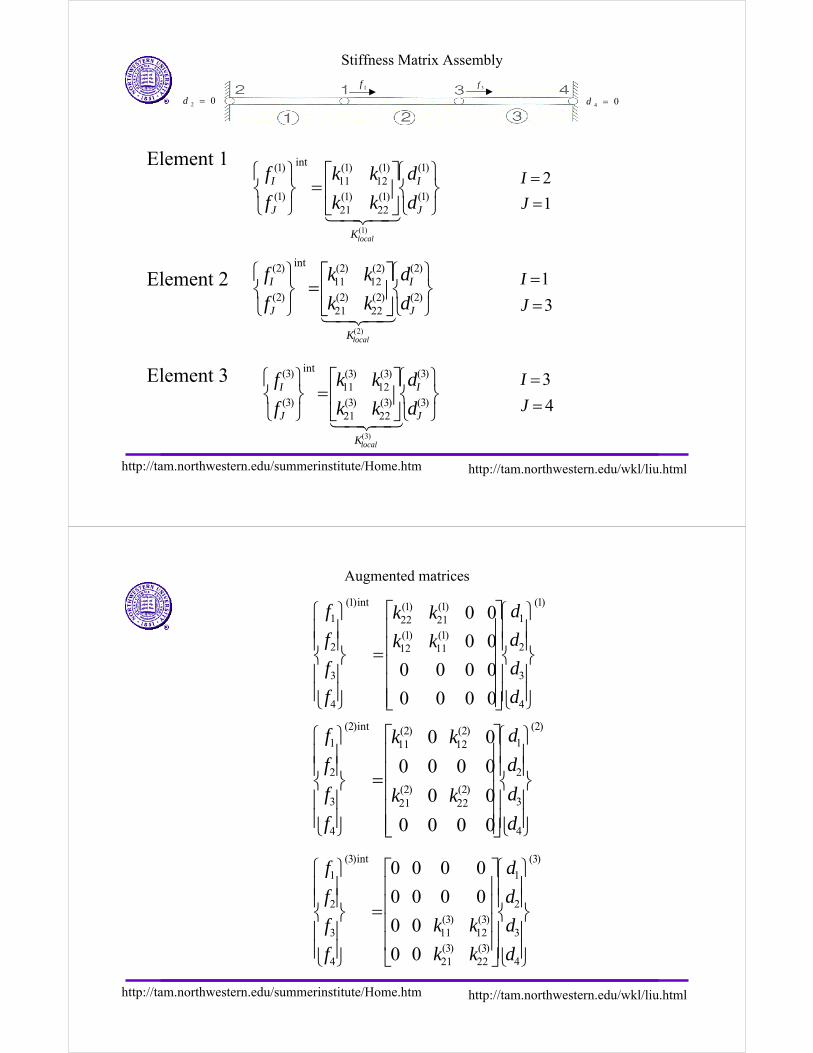
Stiffness Matrix Assembly
Element 1
Element 2
Element 3
⎭⎬⎫
⎩⎨⎧
⎥⎦
⎤⎢⎣
⎡=
⎭⎬⎫
⎩⎨⎧
)1(
)1(
)1(22
)1(21
)1(12
)1(11
int
)1(
)1(
)1(
J
I
K
J
I
d
d
kk
kk
f
f
local
434211
2
==
J
I
⎭⎬⎫
⎩⎨⎧
⎥⎦
⎤⎢⎣
⎡=
⎭⎬⎫
⎩⎨⎧
)2(
)2(
)2(22
)2(21
)2(12
)2(11
int
)2(
)2(
)2(
J
I
K
J
I
d
d
kk
kk
f
f
local
434213
1
==
J
I
⎭⎬⎫
⎩⎨⎧
⎥⎦
⎤⎢⎣
⎡=
⎭⎬⎫
⎩⎨⎧
)3(
)3(
)3(22
)3(21
)3(12
)3(11
int
)3(
)3(
)3(
J
I
K
J
I
d
d
kk
kk
f
f
local
434214
3
==
J
I
1f 3f
02 =d 04 =d
http://tam.northwestern.edu/summerinstitute/Home.htm http://tam.northwestern.edu/wkl/liu.html
Augmented matrices
)1(
4
3
2
1
)1(11
)1(12
)1(21
)1(22
int)1(
4
3
2
1
0000
0000
00
00
⎪⎪⎭
⎪⎪⎬
⎫
⎪⎪⎩
⎪⎪⎨
⎧
⎥⎥⎥⎥⎥
⎦
⎤
⎢⎢⎢⎢⎢
⎣
⎡
=
⎪⎪⎭
⎪⎪⎬
⎫
⎪⎪⎩
⎪⎪⎨
⎧
d
d
d
d
kk
kk
f
f
f
f
)2(
4
3
2
1
)2(22
)2(21
)2(12
)2(11
int)2(
4
3
2
1
0000
00
0000
00
⎪⎪⎭
⎪⎪⎬
⎫
⎪⎪⎩
⎪⎪⎨
⎧
⎥⎥⎥⎥⎥
⎦
⎤
⎢⎢⎢⎢⎢
⎣
⎡
=
⎪⎪⎭
⎪⎪⎬
⎫
⎪⎪⎩
⎪⎪⎨
⎧
d
d
d
d
kk
kk
f
f
f
f
)3(
4
3
2
1
)3(22
)3(21
)3(12
)3(11
int)3(
4
3
2
1
00
00
0000
0000
⎪⎪⎭
⎪⎪⎬
⎫
⎪⎪⎩
⎪⎪⎨
⎧
⎥⎥⎥⎥
⎦
⎤
⎢⎢⎢⎢
⎣
⎡
=
⎪⎪⎭
⎪⎪⎬
⎫
⎪⎪⎩
⎪⎪⎨
⎧
d
d
d
d
kk
kk
f
f
f
f
http://tam.northwestern.edu/summerinstitute/Home.htm http://tam.northwestern.edu/wkl/liu.html
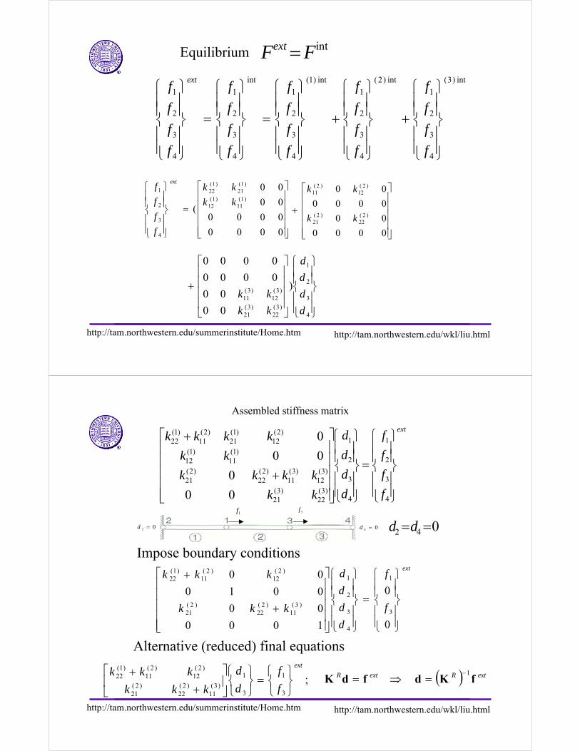
Equilibrium intFFext =int)3(
4
3
2
1
int)2(
4
3
2
1
int)1(
4
3
2
1
int
4
3
2
1
4
3
2
1
⎪⎪⎭
⎪⎪⎬
⎫
⎪⎪⎩
⎪⎪⎨
⎧
+
⎪⎪⎭
⎪⎪⎬
⎫
⎪⎪⎩
⎪⎪⎨
⎧
+
⎪⎪⎭
⎪⎪⎬
⎫
⎪⎪⎩
⎪⎪⎨
⎧
=
⎪⎪⎭
⎪⎪⎬
⎫
⎪⎪⎩
⎪⎪⎨
⎧
=
⎪⎪⎭
⎪⎪⎬
⎫
⎪⎪⎩
⎪⎪⎨
⎧
f
f
f
f
f
f
f
f
f
f
f
f
f
f
f
f
f
f
f
fext
⎥⎥⎥⎥⎥
⎦
⎤
⎢⎢⎢⎢⎢
⎣
⎡
=
⎪⎪⎭
⎪⎪⎬
⎫
⎪⎪⎩
⎪⎪⎨
⎧
0000
0000
00
00
()1(
11)1(
12
)1(21
)1(22
4
3
2
1
kk
kk
f
f
f
fext
⎥⎥⎥⎥⎥
⎦
⎤
⎢⎢⎢⎢⎢
⎣
⎡
+
0000
00
0000
00
)2(22
)2(21
)2(12
)2(11
kk
kk
⎪⎪⎭
⎪⎪⎬
⎫
⎪⎪⎩
⎪⎪⎨
⎧
⎥⎥⎥⎥
⎦
⎤
⎢⎢⎢⎢
⎣
⎡
+
4
3
2
1
)3(22
)3(21
)3(12
)3(11
)
00
00
0000
0000
d
d
d
d
kk
kk
http://tam.northwestern.edu/summerinstitute/Home.htm http://tam.northwestern.edu/wkl/liu.html
Assembled stiffness matrix
ext
f
f
f
f
d
d
d
d
kk
kkkk
kk
kkkk
⎪⎪⎭
⎪⎪⎬
⎫
⎪⎪⎩
⎪⎪⎨
⎧
=
⎪⎪⎭
⎪⎪⎬
⎫
⎪⎪⎩
⎪⎪⎨
⎧
⎥⎥⎥⎥⎥
⎦
⎤
⎢⎢⎢⎢⎢
⎣
⎡
+
+
4
3
2
1
4
3
2
1
)3(22
)3(21
)3(12
)3(11
)2(22
)2(21
)1(11
)1(12
)2(12
)1(21
)2(11
)1(22
00
0
00
0
Impose boundary conditions
042 ==dd
ext
f
f
d
d
d
d
kkk
kkk
⎪⎪⎭
⎪⎪⎬
⎫
⎪⎪⎩
⎪⎪⎨
⎧
=
⎪⎪⎭
⎪⎪⎬
⎫
⎪⎪⎩
⎪⎪⎨
⎧
⎥⎥⎥⎥⎥
⎦
⎤
⎢⎢⎢⎢⎢
⎣
⎡
+
+
0
0
1000
00
0010
00
3
1
4
3
2
1
)3(11
)2(22
)2(21
)2(12
)2(11
)1(22
Alternative (reduced) final equations
;3
1
3
1
)3(11
)2(22
)2(21
)2(12
)2(11
)1(22
ext
f
f
d
d
kkk
kkk
⎭⎬⎫
⎩⎨⎧
=⎭⎬⎫
⎩⎨⎧
⎥⎦
⎤⎢⎣
⎡
++
1f 3f
02 =d 04 =d
( ) extRextR fKdfdK1−
=⇒=
http://tam.northwestern.edu/summerinstitute/Home.htm http://tam.northwestern.edu/wkl/liu.html
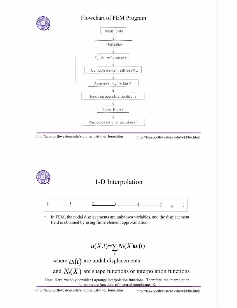
Flowchart of FEM Program
http://tam.northwestern.edu/summerinstitute/Home.htm http://tam.northwestern.edu/wkl/liu.html
1-D Interpolation
• In FEM, the nodal displacements are unknown variables, and the displacement field is obtained by using finite element approximation.
( , ) ( ) ( )I I
INu X t X u t=∑
where are nodal displacements
and are shape functions or interpolation functions
( )Iu t( )IN X
Note: Here, we only consider Lagrange interpolation functions. Therefore, the interpolation functions are functions of material coordinates X.
http://tam.northwestern.edu/summerinstitute/Home.htm http://tam.northwestern.edu/wkl/liu.html
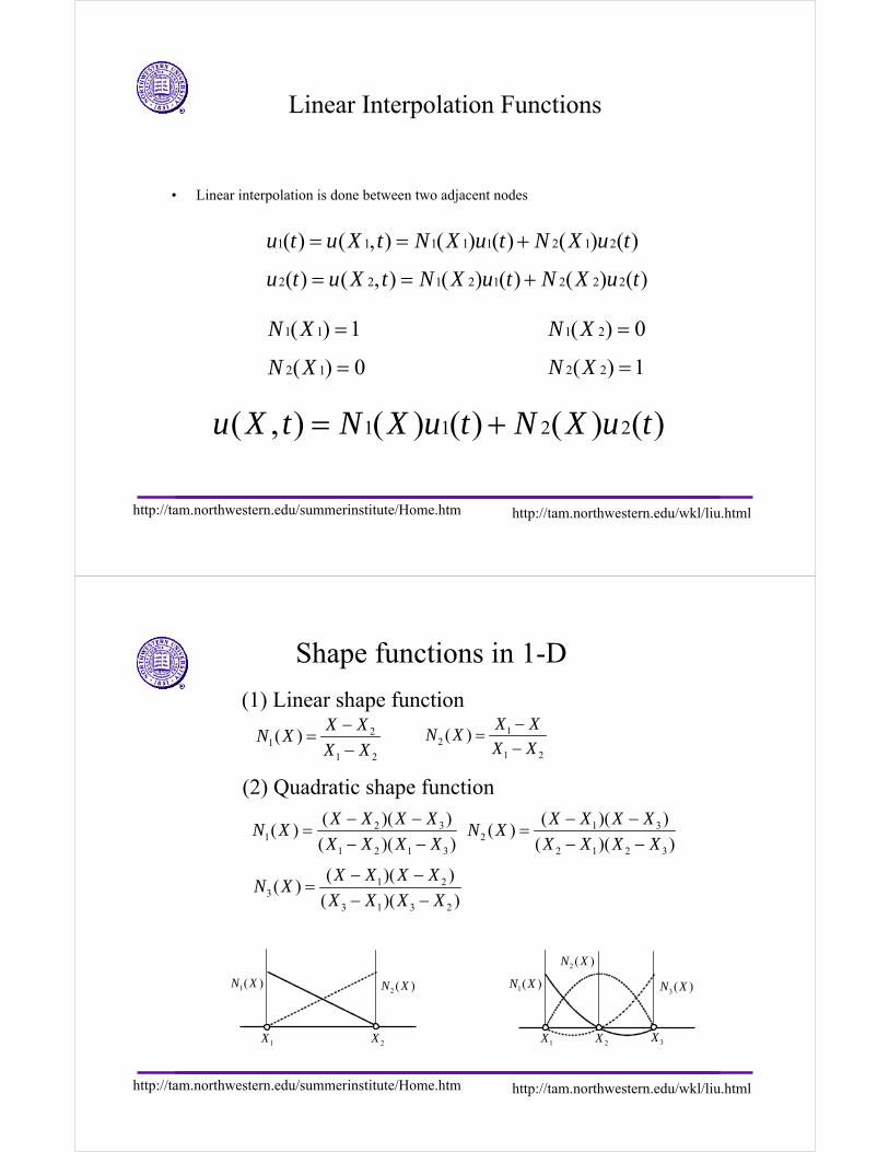
Linear Interpolation Functions
• Linear interpolation is done between two adjacent nodes
1 1 2 2( , ) ( ) ( ) ( ) ( )u X t N X u t N X u t= +
1 1 1 1 1 2 1 2( ) ( , ) ( ) ( ) ( ) ( )u t u X t N X u t N X u t= = +
2 2 1 2 1 2 2 2( ) ( , ) ( ) ( ) ( ) ( )u t u X t N X u t N X u t= = +
2 1( ) 0N X =
1 1( ) 1N X = 1 2( ) 0N X =
2 2( ) 1N X =
http://tam.northwestern.edu/summerinstitute/Home.htm http://tam.northwestern.edu/wkl/liu.html
Shape functions in 1-D
(1) Linear shape function2
11 2
( )X X
N XX X
−=
−1
21 2
( )X X
N XX X
−=
−
1 32
2 1 2 3
( )( )( )
( )( )
X X X XN X
X X X X
− −=
− −
(2) Quadratic shape function
2 31
1 2 1 3
( )( )( )
( )( )
X X X XN X
X X X X
− −=
− −
1 23
3 1 3 2
( )( )( )
( )( )
X X X XN X
X X X X
− −=
− −
1( )N X2 ( )N X
1X 2X
1( )N X3( )N X
2 ( )N X
1X 3X2X
http://tam.northwestern.edu/summerinstitute/Home.htm http://tam.northwestern.edu/wkl/liu.html
1-D Lagrange Polynomials
11
1
( )
( )( )
nen
b
bb anen
a nen
a b
bb a
l
ξ ξ
ξξ ξ
=≠−
=≠
−
=−
∏
∏
order of polynomial: nen-1
the following is the general function:
http://tam.northwestern.edu/summerinstitute/Home.htm http://tam.northwestern.edu/wkl/liu.html
2 node 1-D Lagrange Polynomial
• nen=2; order=nen-1=1
2111
1 2
( ) ( 1) 1( ) (1 )
( ) ( 1 1) 2l N
ξ ξ ξξ ξξ ξ
− −= = = − =
− − −
1122
2 1
( ) ( 1) 1( ) (1 )
( ) (1 1) 2l N
ξ ξ ξξ ξξ ξ
− += = = + =
− +
21
1
( ) ( )a aa
X l Xξ ξ=
= ∑
http://tam.northwestern.edu/summerinstitute/Home.htm http://tam.northwestern.edu/wkl/liu.html
3 node 1-D Lagrange Polynomial
• nen=3; order=nen-1=2
2 3211
1 2 1 3
( )*( ) 1( ) ( 1)
( )*( ) 2l N
ξ ξ ξ ξξ ξ ξξ ξ ξ ξ
− −= = − =
− −
1 3222
2 1 2 3
( )*( ) 1( ) (1 )
( )*( ) 2l N
ξ ξ ξ ξξ ξ ξξ ξ ξ ξ
− −= = + =
− −
32
1
( ) ( )a aa
X l Xξ ξ=
= ∑
2 23 ( ) 1l ξ ξ= −
http://tam.northwestern.edu/summerinstitute/Home.htm http://tam.northwestern.edu/wkl/liu.html
Finite Element Interpolation in 2-D
For each element, we define
44332211 uNuNuNuNu +++=
44332211 vNvNvNvNv +++=
∑=
= ⎭⎬⎫
⎩⎨⎧
=⎭⎬⎫
⎩⎨⎧ 4
1
NEN
I I
II v
uN
v
u
Shape functions are defined in such a way thatIN
IJJI xN δ=)(Bi-linear interpolation
xyayaxaau 3210 +++=xybybxbbv 3210 +++=
http://tam.northwestern.edu/summerinstitute/Home.htm http://tam.northwestern.edu/wkl/liu.html
2-D Lagrange Polynomials
1 1 2 2 3 3 4 4( , ) ( , ) ( , ) ( , ) ( , )X N X N X N X N Xξ η ξ η ξ η ξ η ξ η= + + +
remember that
( , )I J J IJN ξ η δ=
1 1 1
1 1( , ) ( ) ( ) (1 ) (1 )
2 2N l lξ η ξ η ξ η= = − −
2 2 1
1 1( , ) ( ) ( ) (1 ) (1 )
2 2N l lξ η ξ η ξ η= = + −
3 2 2
1 1( , ) ( ) ( ) (1 ) (1 )
2 2N l lξ η ξ η ξ η= = + +
4 1 2
1 1( , ) ( ) ( ) (1 ) (1 )
2 2N l lξ η ξ η ξ η= = − +
http://tam.northwestern.edu/summerinstitute/Home.htm http://tam.northwestern.edu/wkl/liu.html
Section IIINONLINEAR ELASTICITY
Linear Statics
Nonlinear Statics
ext
F
FKd =int
known
extFF =int
where is a nonlinear function of d
For elastostatics,
Nonlinear algebraic equations to be solved
intF
)(int dNF =
http://tam.northwestern.edu/summerinstitute/Home.htm http://tam.northwestern.edu/wkl/liu.html
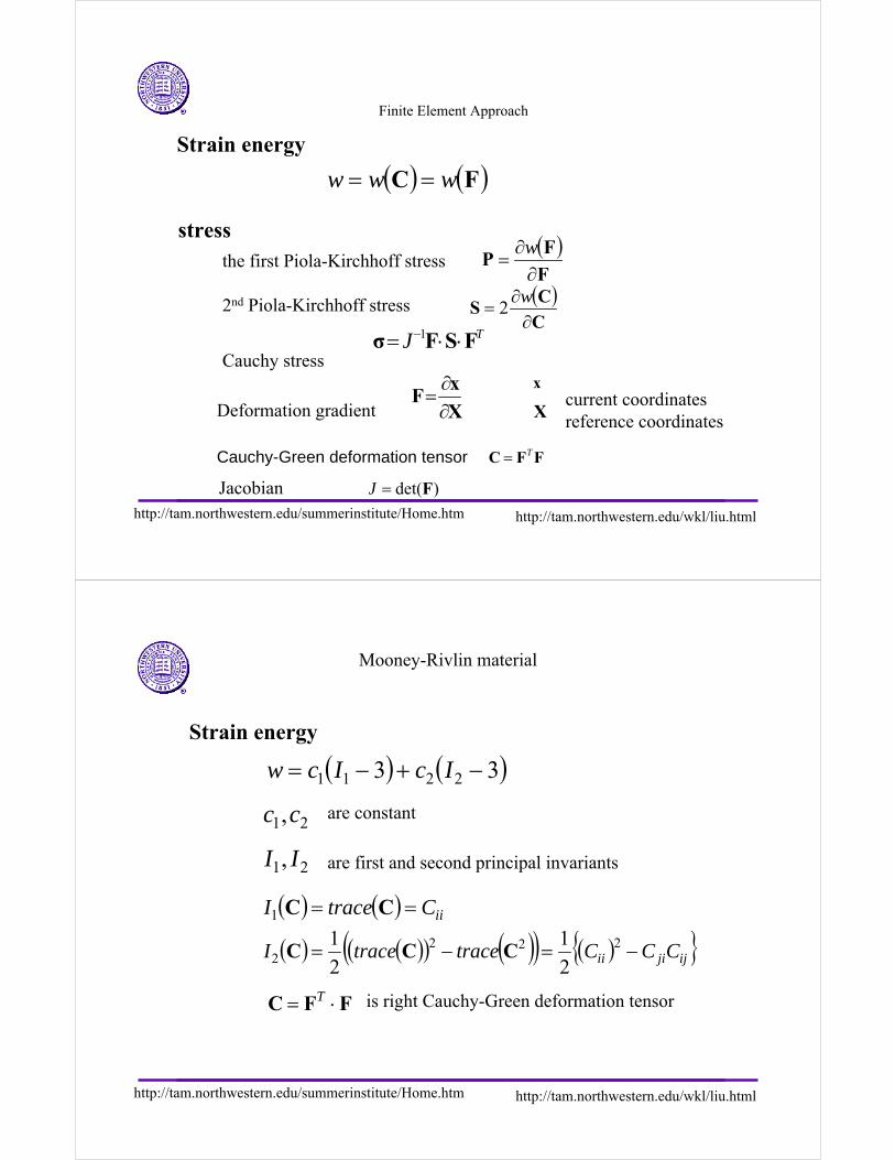
Finite Element Approach
TJ FSFσ ⋅⋅= −1
XX
xF
∂∂
=
Strain energy
stress
( ) ( )FC www ==
the first Piola-Kirchhoff stress( )F
FP
∂∂
=w
( )C
CS
∂∂
=w
22nd Piola-Kirchhoff stress
Cauchy stress
Deformation gradientcurrent coordinatesreference coordinates
x
)det(F=JJacobian
FFC T=Cauchy-Green deformation tensor
http://tam.northwestern.edu/summerinstitute/Home.htm http://tam.northwestern.edu/wkl/liu.html
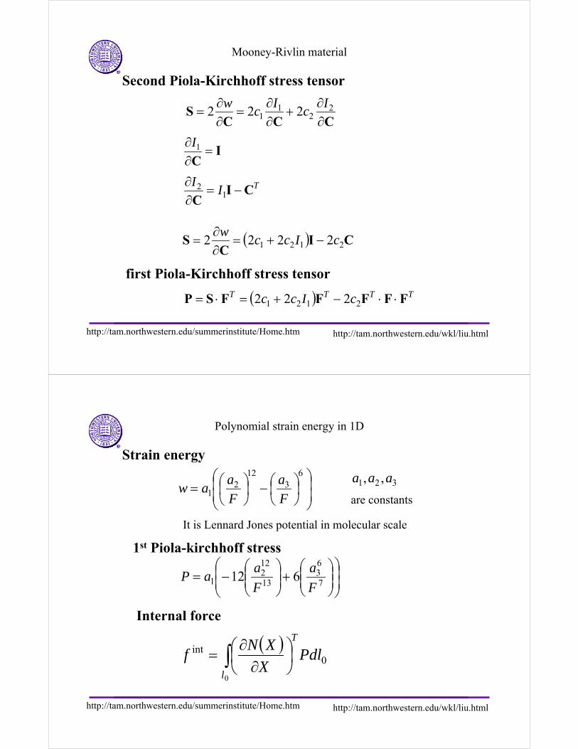
Mooney-Rivlin material
Strain energy
( ) ( )33 2211 −+−= IcIcw
( ) ( ) iiCtraceI == CC1
FFC ⋅= T
21,cc are constant
21, II are first and second principal invariants
( ) ( )( ) ( )( ) ( ) ijjiii CCCtracetraceI −=−= 2222 2
1
2
1CCC
is right Cauchy-Green deformation tensor
http://tam.northwestern.edu/summerinstitute/Home.htm http://tam.northwestern.edu/wkl/liu.html
Mooney-Rivlin material
Second Piola-Kirchhoff stress tensor
CCCS
∂∂
+∂∂
=∂∂
= 22
11 222
Ic
Ic
w
IC
=∂∂ 1I
TII
CIC
−=∂∂
12
( ) CIC
S 2121 2222 cIccw
−+=∂∂
=
( ) TTTT cIcc FFFFFSP ⋅⋅−+=⋅= 2121 222
first Piola-Kirchhoff stress tensor
http://tam.northwestern.edu/summerinstitute/Home.htm http://tam.northwestern.edu/wkl/liu.html
Polynomial strain energy in 1D
Strain energy
⎟⎟⎠
⎞⎜⎜⎝
⎛⎟⎠⎞
⎜⎝⎛−⎟
⎠⎞
⎜⎝⎛=
63
122
1 F
a
F
aaw
It is Lennard Jones potential in molecular scale
1st Piola-kirchhoff stress
⎟⎟⎠
⎞⎜⎜⎝
⎛⎟⎟⎠
⎞⎜⎜⎝
⎛+⎟⎟
⎠
⎞⎜⎜⎝
⎛−= 7
63
13
122
1 612F
a
F
aaP
321 ,, aaa
are constants
Internal force
( )0
int
0
PdlX
XNf
l
T
∫ ⎟⎠⎞
⎜⎝⎛
∂∂
=
http://tam.northwestern.edu/summerinstitute/Home.htm http://tam.northwestern.edu/wkl/liu.html
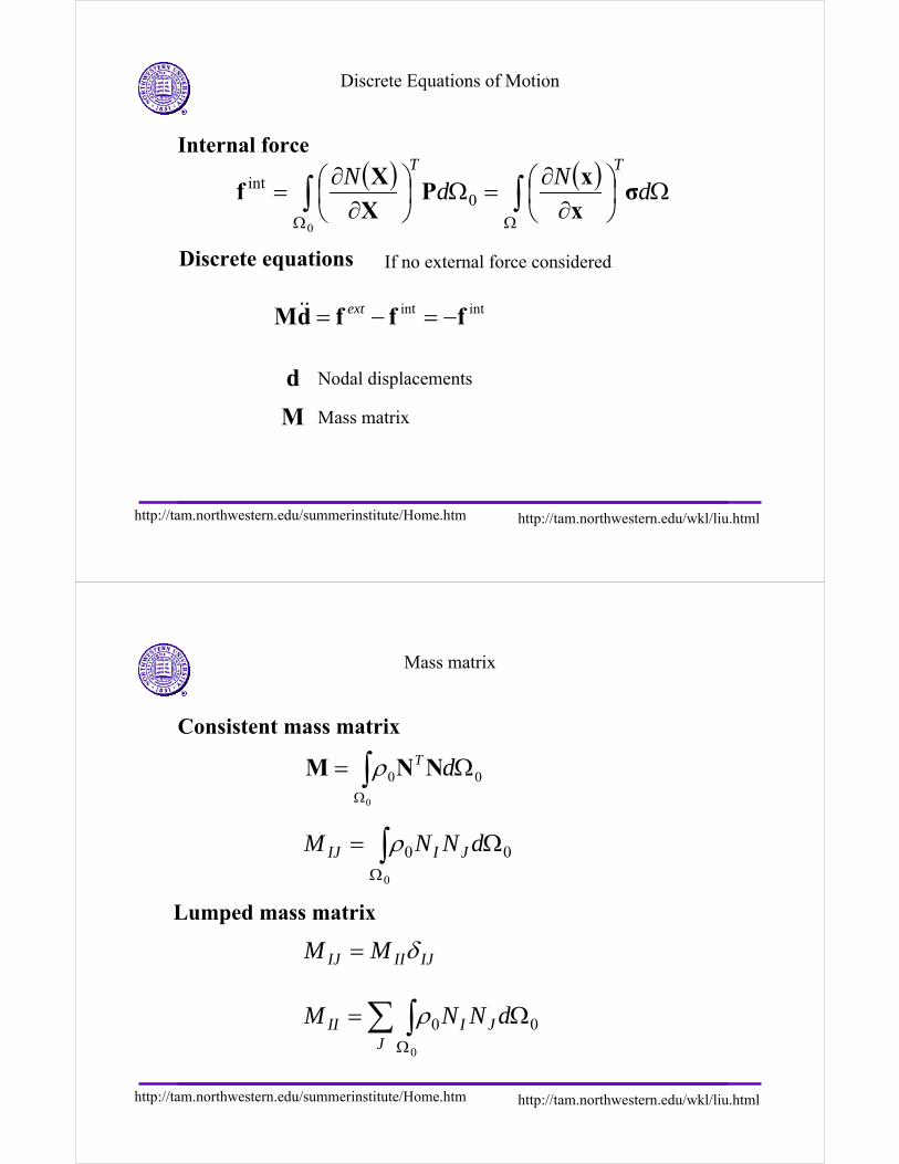
Discrete Equations of Motion
Internal force
Discrete equations
( ) ( )Ω⎟
⎠⎞
⎜⎝⎛
∂∂
=Ω⎟⎠⎞
⎜⎝⎛
∂∂
= ∫∫ΩΩ
dN
dN
TT
σx
xP
X
Xf 0
int
0
If no external force considered
intint fffdM −=−= ext&&
Nodal displacements
Mass matrixM
d
http://tam.northwestern.edu/summerinstitute/Home.htm http://tam.northwestern.edu/wkl/liu.html
Mass matrix
Consistent mass matrix
Lumped mass matrix
00
0
Ω= ∫Ω
dT NNM ρ
00
0
Ω= ∫Ω
dNNM JIIJ ρ
IJIIIJ MM δ=
∑ ∫ Ω=ΩJ
JIII dNNM 00
0
ρ
http://tam.northwestern.edu/summerinstitute/Home.htm http://tam.northwestern.edu/wkl/liu.html
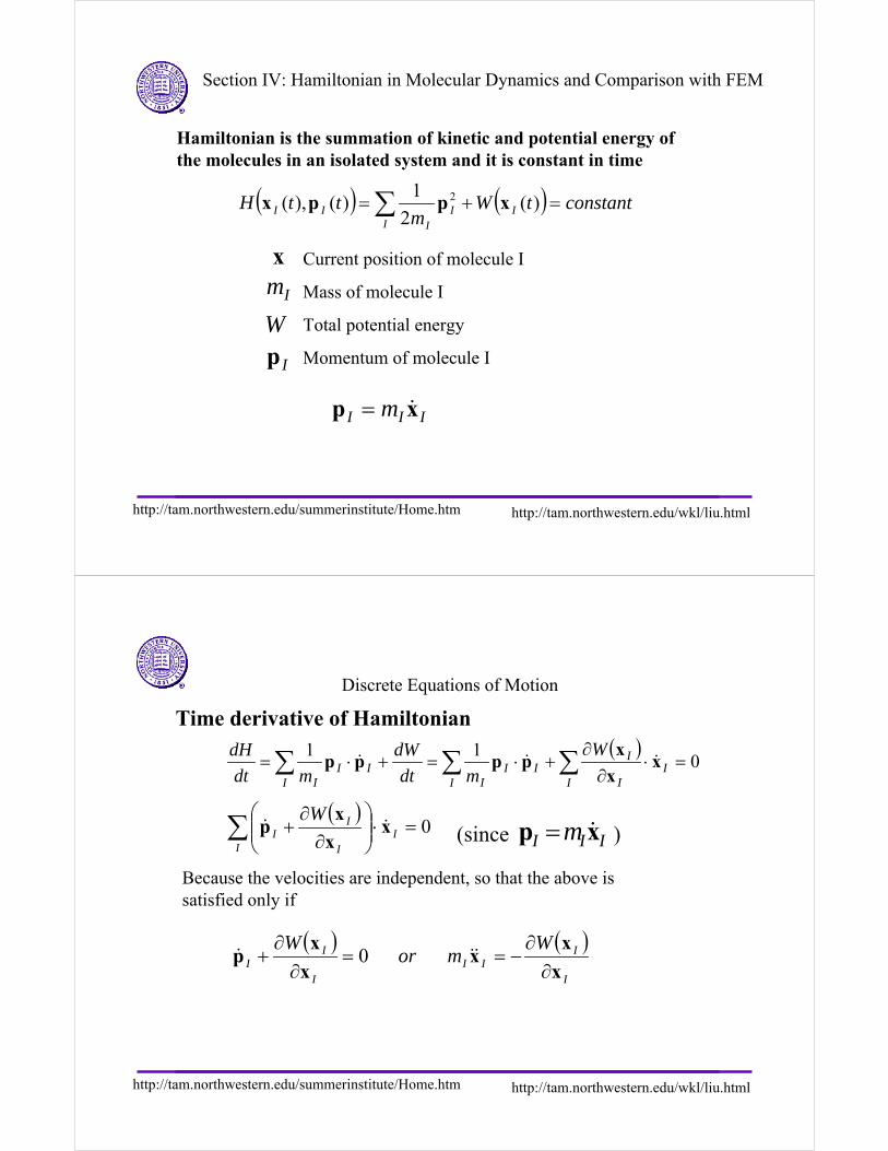
Section IV: Hamiltonian in Molecular Dynamics and Comparison with FEM
Hamiltonian is the summation of kinetic and potential energy of the molecules in an isolated system and it is constant in time
Current position of molecule Ix
( ) ( ) constanttWm
ttH II
II
II =+= ∑ )(2
1)(),( 2 xppx
Im Mass of molecule I
Momentum of molecule IIpTotal potential energyW
III m xp &=
http://tam.northwestern.edu/summerinstitute/Home.htm http://tam.northwestern.edu/wkl/liu.html
Discrete Equations of Motion
Time derivative of Hamiltonian( )
011
=⋅∂
∂+⋅=+⋅= ∑∑∑
II
I
I
III
IIII
I
W
mdt
dW
mdt
dHx
x
xpppp &&&
( )0=⋅⎟⎟
⎠
⎞⎜⎜⎝
⎛∂
∂+∑ I
I I
II
Wx
x
xp &&
Because the velocities are independent, so that the above is satisfied only if
( ) ( )I
III
I
II
Wmor
W
x
xx
x
xp
∂∂
−==∂
∂+ &&& 0
III m xp &=(since )
http://tam.northwestern.edu/summerinstitute/Home.htm http://tam.northwestern.edu/wkl/liu.html
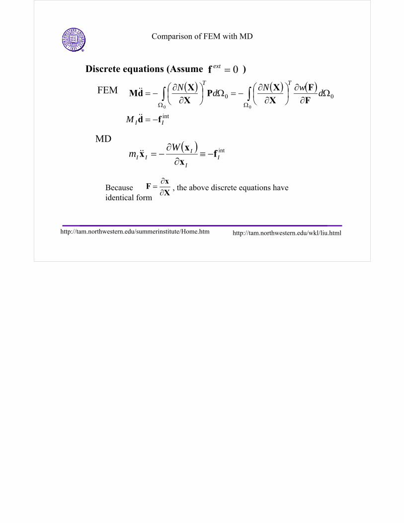
Comparison of FEM with MD
Discrete equations (Assume )
( ) ( ) ( )
int
00
00
II
TT
M
dwN
dN
fd
F
F
X
XP
X
XdM
−=
Ω∂
∂⎟⎠⎞
⎜⎝⎛
∂∂
−=Ω⎟⎠⎞
⎜⎝⎛
∂∂
−= ∫∫ΩΩ
&&
&&
( ) intI
I
III
Wm f
x
xx −≡
∂∂
−=&&
Because , the above discrete equations have identical form
X
xF
∂∂
=
FEM
MD
0=extf