Branch trace compression for snapshot-based …krste/papers/bpred-ispass06.pdfBranch Trace Compression for Snapshot-Based Simulation ... a matching software branch predictor to help

In IEEE Int’l Symposium on Performance Analysis of Systems and Software (ISPASS), Austin, TX, March 2006.

Branch Trace Compression for Snapshot-Based Simulation

Kenneth C. Barr and Krste AsanovicMIT Computer Science and Artificial Intelligence Laboratory

The Stata Center, 32 Vassar Street, Cambridge, MA 02139{kbarr, krste}@csail.mit.edu

Abstract

We present a scheme to compress branch trace informationfor use in snapshot-based microarchitecture simulation. Thecompressed trace can be used to warm any arbitrary branchpredictor’s state before detailed microarchitecture simulationof the snapshot. We show that compressed branch traces re-quire less space than snapshots of concrete predictor state. Ourbranch-predictor based compression (BPC) technique uses asoftware branch predictor to provide an accurate model of theinput branch trace, requiring only mispredictions to be storedin the compressed trace file. The decompressor constructsa matching software branch predictor to help reconstruct theoriginal branch trace from the record of mispredictions. Eval-uations using traces from the Journal of ILP branch predictorcompetition show we achieve compression rates of 0.013–0.72bits/branch (depending on workload), which is up to 210× bet-ter than gzip; up to 52× better than the best general-purposecompression techniques; and up to 4.4× better than recentlypublished, more general trace compression techniques. More-over, BPC-compressed traces can be decompressed in less timethan corresponding traces compressed with other methods.

1. Introduction

As full-system simulation becomes more popular andworkloads become longer, methodologies such as statisticalsimulation and phase detection have been proposed to pro-duce reliable performance analysis in a small amount of time[12, 21, 22, 30]. When such techniques are adopted, the bulkof simulation time is spent fast-forwarding the simulator torelevant points in a program rather than performing detailedcycle-accurate simulation. To amortize the cost of lengthy fast-forwarding, snapshots containing architectural state can be cap-tured at each sample point [2, 29]. The snapshots can thenbe used to initialize different machine configurations withoutrepeating the fast-forwarding. Microarchitectural state can bereconstructed using a “detailed warming” phase before resultsare gathered at each sample point, but if the microarchitecturalstate is large, such as for caches and branch predictors, the timerequired for detailed warming can be prohibitive.

Microarchitectural state can also be captured in the snap-shot, but this will then require regeneration of the snapshot

every time a microarchitectural feature is modified. Ideally,the snapshots should be microarchitecture independent, to sup-port microarchitectural exploration with a standard set of storedsnapshots. For caches, various microarchitecture-independentsnapshot schemes have been proposed, which take advantageof the simple mapping of memory addresses to cache sets[1, 13, 27, 28]. Branch predictors, however, are much more dif-ficult to handle in the same way, as the common use of globalbranch histories smears the effect of a single branch addressacross many locations in a branch predictor. One possibility isto store microarchitectural state snapshots for a set of of poten-tial branch predictors, but this limits flexibility and increasessnapshot size, particularly when many samples are taken of along-running multiprocessor application. We explore an alter-native approach in this paper, which is to store a compressedversion of the complete branch trace in the snapshot. This ap-proach is microarchitecture-independent because any branchpredictor can be initialized before detailed simulation beginsby uncompressing and replaying the branch trace.

The main contribution of our paper is a branch predictor-based compression (BPC) scheme, which exploits a softwarebranch predictor in the compressor and decompressor to reducethe size of the compressed branch trace snapshot. We show thatwhen BPC is used, the snapshot library can require less spacethan one which stores just a single concrete predictor configu-ration, and it allows us to simulate any sort of branch predictor.

We describe the structure of our BPC compressor in Sec-tion 2. In Section 3, we examine the improvement of our tech-nique versus general-purpose compressors and snapshots, andwe show how it scales with program size in terms of storageand performance. Section 4 notes related work in compressionand simulation acceleration, and Section 5 concludes.

2. Design of a branch predictor-basedtrace compressor

In general, lossless data compression can be partitionedinto two phases: modeling and coding. The modeling phaseattempts to predict the data symbols. For each symbol in theinput text, the compressor expresses any differences from themodel. The coding phase creates concise codewords to repre-sent these differences in as few bits as possible. BPC uses a

1


collection of internal predictors to create an accurate, adaptivemodel of branch behavior. We delegate the coding step to ageneral-purpose compressor.

To model the direction and targets of branches in a trace,we can draw on years of research in high accuracy hardwarebranch predictors. When using branch predictors as models insoftware, we have two obvious advantages over hardware pre-dictors. First, the severe constraints that usually apply to branchprediction table sizes disappear; second, a fast functional sim-ulator (which completes the execution of an entire instructionbefore proceeding) can provide oracle information to the pre-dictor such as computed branch targets and directions. We usethe accurate predictions from software models to reduce theamount of information passed to the coder. When the modelcan predict many branches in a row, we do not have to includethese branches in the compressor output; we only have to ex-press the fact that the information is contained in the model.

2.1. Structure

Figure 1 shows the different components in our system. Abenchmark is simulated with a fast functional simulator, andinformation about branches is passed to the BPC Compres-sor. The BPC Compressor processes the branch stream, filtersit through a general-purpose compressor, and creates a com-pressed trace on disk. We will show momentarily how the BPCCompressor can improve its compression ratios by using itsown output as input to compress the next branch.

We define a concrete branch predictor to be a predictorwith certain fixed parameters. These parameters may includesize of global history, number of branch target buffer (BTB)entries, indexing functions, et cetera. To evaluate the perfor-mance of various concrete branch predictors, we retrieve thecompressed trace from disk, remove the general-purpose com-pression layer, and process it with the BPC Decompressor. Thestructure of the decompressor is identical to that of the com-pressor. The output of the BPC Decompressor is used to up-date state in each concrete predictor used in the experiment.Branches later in the trace will overwrite entries in the concretepredictor according to its policies.

The particular collection of internal predictors has nothingto do with the concrete branch predictors that BPC will warm.The implementation of BPC merely uses predictors to aid com-pression of the complete branch trace which, by its nature, canbe used to fill any branch predictor with state based on infor-mation in the trace. Furthermore, the precise construction of aBPC scheme is up to the implementor who may choose to sac-rifice compression for speed and simplicity or vice versa. Wemerely describe what appears to be a happy medium.

Note this implementation differs from other proposedvalue predictor-based compression (VPC) techniques, whichfeed several predictors in parallel and emit a code indicatingwhich predictor is correct [4, 26]. We have found that, for ourdatasets of branch traces, indicating in the output stream whichone of a set of predictors has succeeded results in a stream ofindicator codes which is itself difficult to compress.

Benchmark

Simulator

BPCDecompressorCompressor

ConcreteBranchPredictors

Functional

BPC

decompressorGeneral purposeGeneral purpose

compressor

CompressedTrace

Figure 1. System diagram. The compressed trace is storedon disk until it is needed to reconstruct concrete branchpredictors.

2.2. Branch notation and representation

Before getting into the details of the compressor, we de-scribe the information stored in the compressed trace and in-troduce some notation used in this paper.

Using the Championship Branch Prediction (CBP) frame-work [26], the uncompressed branch traces in our study con-sist of fixed-length branch records as shown in Table 1. Eachbranch record contains the current instruction address, the fall-through instruction address (not obvious in CISC ISAs), thebranch target, and type (not mutually exclusive) which indi-cates whether the branch is a call, return, indirect, or con-ditional. The branch records are generated by a functionalsimulator which can resolve the branch target and provide ataken/not-taken bit. The taken bit is stored in a one-byte fieldto facilitate compression via popular bytewise algorithms suchas gzip [11], bzip2 [23], or PPMd [24].

Table 1. Format of branch records.

field size(Bytes)

instruction address 4fall-through instruction address 4branch target address 4taken 1is indirect is conditional is call is return 1

2


Rather than predicting the direction and target of the cur-rent branch, Bn, as in a hardware direction predictor and branchtarget buffer (BTB), we predict information about the nextbranch, Bn+1. We denote the actual branch stream as B0..kand predicted branches as β0..k. If the predictor proves correct(βn+1 = Bn+1) we concisely note that fact and need not providethe entire Bn+1 branch record. Furthermore, we use βn+1 toproduce βn+2..n+i for as large an i as possible. This allows us touse a single symbol to inform the decompressor that i chainedpredictions will be correct.

Figure 2 depicts an example using this notation. GivenBn we must provide information about βn+1. In this case, wehave predicted βn+1 to be not-taken with a specific fall-throughaddress. If these are correct predictions, BPC can continue bychaining: using βn+1 as input to request predictions about βn+2.The longer the chain of correct predictions, the less informationhas to be written by the compressor.

BasicBlock 1 Block 2

Basic

Block 3Basic

Bn.branch target

βn+1.fall through

βn+2

βn+1Bn

Figure 2. Graphic depiction of our notation.

The output of the compressor is a list of pairs. The firstelement indicates the number of correct predictions that canbe made beginning with a given branch; the second elementcontains the data for the branch that cannot be predicted. Anexample output is shown in Table 2. As in most branch traces,the example shows that the first few branches cannot be pre-dicted and must be transmitted in their entirety. Eventually thecompressor outputs B10 and uses B10 as an input to its internalpredictors, coming up with a prediction, β11. Comparing β11 tothe next actual branch, B11, a match is detected. This processcontinues until the internal predictors fail to guess the incomingbranch (at B24). Thus, we output “13” to indicate that, by chain-ing predictor output to the next prediction’s input, 13 branchesin a row will be predicted correctly, but β24 6= B24. We emit B24and repeat the process.

We store the output in two separate files and use a general-purpose compressor (such as gzip or bzip2) to catch patternsthat we have missed and to encode the reduced set of symbols.

Table 2. Example compressor output.

skip amount branch record

0 B00 B10 B2... ...0 B1013 B24

2.3. Algorithm and implementation details

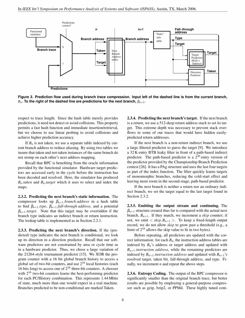
The internal structure of a BPC Compressor is shown inFigure 3. Each box corresponds to one predictor. When multi-ple predictors are present at a stage, only one is consulted. InBPC, the criteria for choosing a predictor stems from branchtype which expresses characteristics of the branch such aswhether it is a return instruction or if it is conditional. The de-tails of how type determines predictor selection are explainedin Sections 2.3.3 and 2.3.4.

The description below refers to the steady-state operation.We do not describe handling of the first and last branch, nordo we detail the resetting of the skip counter. These cornercases are addressed in our code. We use diff to ensure acompressed trace can be uncompressed correctly.

Initially, a known address, target, and taken bit of Bn arereceived from the functional simulator and used to predict theaddress of βn+1. This address is used to look up static informa-tion about βn+1 including its fall-through address, type, and tar-get. In the absence of context switches or self-modifying code,the branch address corresponds directly with a type and fall-through address. If the branch target is not computed, a givenbranch address always has the same branch target. The typeprediction helps the direction predictor decide whether βn+1 isa taken branch. The type also helps the target predictor makeaccurate predictions. Once components of βn+1 have been pre-dicted, it can be used to generate a prediction for βn+2 and soon. Before continuing, the predictors are updated with correctdata for Bn+1 provided by the simulator.

2.3.1. Predicting the next branch address. Normally,branch targets must be predicted, but in the case of BPC,they are known by the functional simulator. Instead, we mustpredict the address of the next branch. Since the next branchseen by a program is the first branch to appear after reaching atarget, knowing the target allows us to know the next branch. Ifthe branch is not taken, the next branch should appear shortlya few instructions later. This prediction will be 100% correctunless we are faced with self-modifying code or processswaps.

If Bn is a taken branch, we use a simple mapping of currentbranch target to next branch address. This map can be consid-ered a Last-1-Value predictor or a cache. Our map is imple-mented with a 256K-entry hash table. The hash tables and fixedsized predictors of BPC provide O(1) read and write time with

3


Fall−throughaddress

Predictionscorrect?

DirectionPredictor

tablesAddressBranchNext

simulatorFunctional

Branch address

n+1

Taken

n

Predictions

1 Target

Branch address Type

Targettableinfo

0

Target

Taken

TargetPredictors(RAS + Indirect)

Branch trace

"Static"

Figure 3. Prediction flow used during branch trace compression. Input left of the dashed line is from the current branch,Bn. To the right of the dashed line are predictions for the next branch, βn+1.

respect to trace length. Since the hash table merely providespredictions, it need not detect or avoid collisions. This propertypermits a fast hash function and immediate insertion/retrieval,but we choose to use linear probing to avoid collisions andachieve higher prediction accuracy.

If Bn is not taken, we use a separate table indexed by cur-rent branch address to reduce aliasing. By using two tables weinsure that taken and not-taken instances of the same branch donot stomp on each other’s next address mapping.

Recall that BPC is benefiting from the oracle informationprovided by the functional simulator. Hardware target predic-tors are accessed early in the cycle before the instruction hasbeen decoded and resolved. Here, the simulator has producedBn.taken and Bn.target which it uses to select and index themaps.

2.3.2. Predicting the next branch’s static information. Thecompressor looks up βn+1.branch address in a hash tableto find βn+1.type, βn+1.fall-through address, and a potentialβn+1.target. Note that this target may be overridden if thebranch type indicates an indirect branch or return instruction.The lookup table is implemented as in Section 2.2.1.

2.3.3. Predicting the next branch’s direction. If the (pre-dicted) type indicates the next branch is conditional, we lookup its direction in a direction predictor. Recall that our soft-ware predictors are not constrained by area or cycle time asin a hardware predictor. Thus, we chose a large variation ofthe 21264-style tournament predictor [15]. We XOR the pro-gram counter with a 16 bit global branch history to access aglobal set of two-bit counters, and use 216 local histories (each16 bits long) to access one of 216 three-bit counters. A chooserwith 216 two-bit counters learns the best-performing predictorfor each PC/History combination. This represents 1.44 Mbitsof state, much more than one would expect in a real machine.Branches predicted to be non-conditional are marked Taken.

2.3.4. Predicting the next branch’s target. If the next branchis a return, we use a 512-deep return address stack to set its tar-get. This extreme depth was necessary to prevent stack over-flows in some of our traces that would have hidden easily-predicted return addresses.

If the next branch is a non-return indirect branch, we usea large filtered predictor to guess the target [9]. We introducea 32 K-entry BTB leaky filter in front of a path-based indirectpredictor. The path-based predictor is a 220 entry version ofthe predictor provided by the Championship Branch Predictioncontest [26]. It has a PAg structure and uses the last four targetsas part of the index function. The filter quickly learns targetsof monomorphic branches, reducing the cold-start effect andleaving more room in the second-stage, path-based predictor.

If the next branch is neither a return nor an ordinary indi-rect branch, we set the target equal to the last target found inSection 2.3.2.

2.3.5. Emitting the output stream and continuing. Theβn+1 structure created thus far is compared with the actual nextbranch, Bn+1. If they match, we increment a skip counter; ifnot, we emit < skip,Bn+1 >. To keep a fixed-length outputrecord, we do not allow skip to grow past a threshold (e.g., alimit of 216 allows the skip value to fit in two bytes).

Before repeating, all predictors are updated with the cor-rect information: for each Bn, the instruction address tables areindexed by Bn’s address or target address and updated withBn+1.instruction address, while the remaining predictors areindexed by Bn+1.instruction address and updated with Bn+1’sresolved target, taken bit, fall-through address, and type. Fi-nally, we increment n and repeat the above steps.

2.3.6. Entropy Coding. The output of the BPC compressor issignificantly smaller than the original branch trace, but betterresults are possible by employing a general-purpose compres-sor such as gzip, bzip2, or PPMd. These highly tuned com-

4


pressors are sometimes able to capture patterns missed by BPCand use Huffman or arithmetic coding to compress the outputfurther.

2.3.7. Decompression Algorithm. The decompressor mustread from these files and output the original branch trace onebranch at a time and in the correct order. The BPC decom-pression process uses the same structures described in Sec-tions 2.3.1–2.3.5 so it can be described quickly. As above, weassume a steady state where we have already read Bn.

After reversing the general-purpose compression, the de-compressor first reads from the skip amount file. If the skipamount is zero, it emits Bn+1 as found in the branch recordfile, and updates its internal predictors using Bn and Bn+1.

If it encounters a non-zero skip amount, it uses previousbranch information to produce the next branch. In other words,to emit Bn+1 it queries its internal predictors with Bn and out-puts the address, fall-through, target, type, and taken informa-tion contained in the internal predictors. Next, the skip amountis decremented, Bn+1 becomes the current branch (Bn), and theprocess repeats. Eventually, the skip amount reaches 0, andthe next branch must be fetched from the input file rather thanemitted by the predictors.

As the decompressor updates its internal predictors usingthe same rules as the compressor, the state matches at everybranch, and the decompressor is guaranteed to produce correctpredictions during the indicated skip intervals. The structureof the decompressor is identical to that of the compressor, sodecompression proceeds in roughly the same time as compres-sion.

Recall that the motivation for compressing a branch traceis to replace concrete branch predictor snapshots for sampling-based simulation. By piping the output of our decompressorinto a concrete branch predictor model, the model becomeswarmed-up with exactly the same state it would have containedhad it been in use all along. Furthermore, the decompressedbranch stream can be directed into multiple concrete branchpredictors so that each may be evaluated during detailed sim-ulation. After each branch is examined it may be discarded tominimize disk usage. Since the trace is generated with a fastnon-speculative model, the predictors do not capture wrong-path effects, but the resulting bias has been shown to be accept-able [30].

3. Evaluation

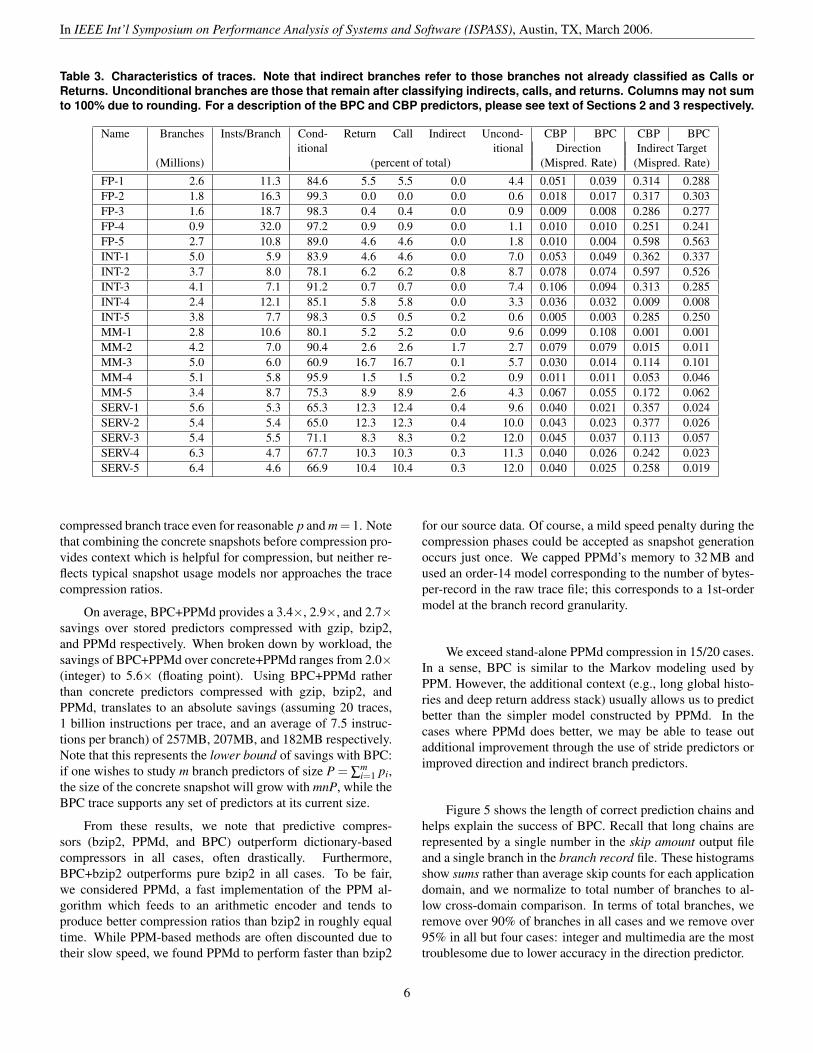
Our simulation framework is based on the CBP compe-tition trace reader which provides static and dynamic informa-tion about each branch in its trace suite. The trace suite consistsof 20 traces from four categories: integer, floating point, server,and multimedia. Each trace contains approximately 30 millioninstructions comprising both user and system activity [26] andexhibiting a wide range of characteristics in terms of branchfrequency and predictability as shown in Table 3. The tracesare used to drive predictors from the competition as well as

custom models. Columns labeled CBP show the direction ac-curacy and indirect target accuracy of the predictors used in theChampionship Branch Prediction trace reader: a gshare predic-tor with a 14-bit global history register, and an indirect targetpredictor in a PAg configuration with 210 entries and a path-length of 4 (bits from the past four targets are hashed with theprogram counter to index into a target table). The BPC columnshows the decreased misprediction rate available to BPC withthe configuration described in Section 2.3.3 and Section 2.3.4.

Using this framework we will show that BPC provides anexcellent level of compression. Not only does a compressedtrace require less space than compressed snapshots, but a BPC-compressed trace is smaller and faster to decompress than othercompression techniques.

3.1. Compression ratio

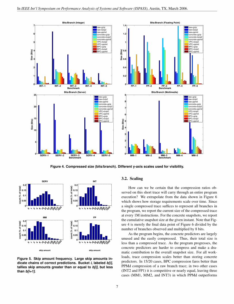
Figure 4 shows the compression ratio resulting from vari-ous methods of branch trace compression for each trace. Traceswere run to completion with snapshots taken every 1M instruc-tions. This sampling interval was found to produce good re-sults on Spec benchmarks [30]. Each trace provides enoughbranches for 29 snapshots. We report bits-per-branch (ratherthan absolute file size or ratio of original size to new size)so that our results are independent from the representation ofbranch records in the input file. From left-to-right we see com-pression ratios for general-purpose compressors; compressedconcrete snapshots; VPC (a similar work which is discussedin Section 3.4); and BPC as described in this paper. We usethe suffix +comp to denote the general-purpose second-stagecompressor.

While slower, bzip2 and PPMd give astonishingly goodresults on raw trace files composed of fixed-length records.In fact, these general-purpose compressors use algorithms thathave a more predictive nature than the dictionary-based gzip.

The three bars labeled “concrete” show the size of a snap-shot containing a single branch predictor roughly approximat-ing that of the Pentium 4: a 4-way, 4096 entry BTB to predicttargets and a 16-bit gshare predictor to predict directions [20].Together the uncompressed size of the concrete predictor is43.6 KB, however we use a bytewise representation and store a97 KB snapshot as it is more amenable to compression than abitwise representation – up to 20% smaller in some cases. Thefigure shows the size of bytewise snapshots after compressionwith gzip, bzip2, and PPMd.

The state of a given branch predictor (a concrete snapshotin our terminology) has constant size of q bytes. However,to have m predictors warmed-up at each of n detailed samplepoints (multiple short samples are desired to capture whole-program behavior), one must store mn q-byte snapshots. Con-crete snapshots are hard to compress so p, the size of q af-ter compression, is roughly constant across snapshots. Sincea snapshot is needed for every sample period, we considerthe cumulative snapshot size: mnp. This cumulative snap-shot grows with m and n. In fact, it grows faster than a BPC-

5


Table 3. Characteristics of traces. Note that indirect branches refer to those branches not already classified as Calls orReturns. Unconditional branches are those that remain after classifying indirects, calls, and returns. Columns may not sumto 100% due to rounding. For a description of the BPC and CBP predictors, please see text of Sections 2 and 3 respectively.

Name Branches Insts/Branch Cond- Return Call Indirect Uncond- CBP BPC CBP BPCitional itional Direction Indirect Target

(Millions) (percent of total) (Mispred. Rate) (Mispred. Rate)

FP-1 2.6 11.3 84.6 5.5 5.5 0.0 4.4 0.051 0.039 0.314 0.288FP-2 1.8 16.3 99.3 0.0 0.0 0.0 0.6 0.018 0.017 0.317 0.303FP-3 1.6 18.7 98.3 0.4 0.4 0.0 0.9 0.009 0.008 0.286 0.277FP-4 0.9 32.0 97.2 0.9 0.9 0.0 1.1 0.010 0.010 0.251 0.241FP-5 2.7 10.8 89.0 4.6 4.6 0.0 1.8 0.010 0.004 0.598 0.563INT-1 5.0 5.9 83.9 4.6 4.6 0.0 7.0 0.053 0.049 0.362 0.337INT-2 3.7 8.0 78.1 6.2 6.2 0.8 8.7 0.078 0.074 0.597 0.526INT-3 4.1 7.1 91.2 0.7 0.7 0.0 7.4 0.106 0.094 0.313 0.285INT-4 2.4 12.1 85.1 5.8 5.8 0.0 3.3 0.036 0.032 0.009 0.008INT-5 3.8 7.7 98.3 0.5 0.5 0.2 0.6 0.005 0.003 0.285 0.250MM-1 2.8 10.6 80.1 5.2 5.2 0.0 9.6 0.099 0.108 0.001 0.001MM-2 4.2 7.0 90.4 2.6 2.6 1.7 2.7 0.079 0.079 0.015 0.011MM-3 5.0 6.0 60.9 16.7 16.7 0.1 5.7 0.030 0.014 0.114 0.101MM-4 5.1 5.8 95.9 1.5 1.5 0.2 0.9 0.011 0.011 0.053 0.046MM-5 3.4 8.7 75.3 8.9 8.9 2.6 4.3 0.067 0.055 0.172 0.062SERV-1 5.6 5.3 65.3 12.3 12.4 0.4 9.6 0.040 0.021 0.357 0.024SERV-2 5.4 5.4 65.0 12.3 12.3 0.4 10.0 0.043 0.023 0.377 0.026SERV-3 5.4 5.5 71.1 8.3 8.3 0.2 12.0 0.045 0.037 0.113 0.057SERV-4 6.3 4.7 67.7 10.3 10.3 0.3 11.3 0.040 0.026 0.242 0.023SERV-5 6.4 4.6 66.9 10.4 10.4 0.3 12.0 0.040 0.025 0.258 0.019

compressed branch trace even for reasonable p and m = 1. Notethat combining the concrete snapshots before compression pro-vides context which is helpful for compression, but neither re-flects typical snapshot usage models nor approaches the tracecompression ratios.

On average, BPC+PPMd provides a 3.4×, 2.9×, and 2.7×savings over stored predictors compressed with gzip, bzip2,and PPMd respectively. When broken down by workload, thesavings of BPC+PPMd over concrete+PPMd ranges from 2.0×(integer) to 5.6× (floating point). Using BPC+PPMd ratherthan concrete predictors compressed with gzip, bzip2, andPPMd, translates to an absolute savings (assuming 20 traces,1 billion instructions per trace, and an average of 7.5 instruc-tions per branch) of 257MB, 207MB, and 182MB respectively.Note that this represents the lower bound of savings with BPC:if one wishes to study m branch predictors of size P = ∑

mi=1 pi,

the size of the concrete snapshot will grow with mnP, while theBPC trace supports any set of predictors at its current size.

From these results, we note that predictive compres-sors (bzip2, PPMd, and BPC) outperform dictionary-basedcompressors in all cases, often drastically. Furthermore,BPC+bzip2 outperforms pure bzip2 in all cases. To be fair,we considered PPMd, a fast implementation of the PPM al-gorithm which feeds to an arithmetic encoder and tends toproduce better compression ratios than bzip2 in roughly equaltime. While PPM-based methods are often discounted due totheir slow speed, we found PPMd to perform faster than bzip2

for our source data. Of course, a mild speed penalty during thecompression phases could be accepted as snapshot generationoccurs just once. We capped PPMd’s memory to 32 MB andused an order-14 model corresponding to the number of bytes-per-record in the raw trace file; this corresponds to a 1st-ordermodel at the branch record granularity.

We exceed stand-alone PPMd compression in 15/20 cases.In a sense, BPC is similar to the Markov modeling used byPPM. However, the additional context (e.g., long global histo-ries and deep return address stack) usually allows us to predictbetter than the simpler model constructed by PPMd. In thecases where PPMd does better, we may be able to tease outadditional improvement through the use of stride predictors orimproved direction and indirect branch predictors.

Figure 5 shows the length of correct prediction chains andhelps explain the success of BPC. Recall that long chains arerepresented by a single number in the skip amount output fileand a single branch in the branch record file. These histogramsshow sums rather than average skip counts for each applicationdomain, and we normalize to total number of branches to al-low cross-domain comparison. In terms of total branches, weremove over 90% of branches in all cases and we remove over95% in all but four cases: integer and multimedia are the mosttroublesome due to lower accuracy in the direction predictor.

6


INT−1 INT−2 INT−3 INT−4 INT−5 0

1

2

3

4

5

6

7

Benchmark

Size

(Bits

)

Bits/Branch (Integer)

raw+gzipraw+bzip2raw+ppmdconcrete+gzipconcrete+bzip2concrete+ppmdVPC+bzip2VPC+ppmdBPC+gzipBPC+bzip2BPC+ppmd

FP−1 FP−2 FP−3 FP−4 FP−5 0

0.2

0.4

0.6

0.8

1

1.2

1.4

Benchmark

Size

(Bits

)

Bits/Branch (Floating Point)


SERV−1 SERV−2 SERV−3 SERV−4 SERV−50

5

10

15

20

25

Benchmark

Size

(Bits

)

Bits/Branch (Server)


MM−1 MM−2 MM−3 MM−4 MM−5 0

1

2

3

4

5

6

7

8

9

Benchmark

Size

(Bits

)

Bits/Branch (Multimedia)


Figure 4. Compressed size (bits/branch). Different y-axis scales used for visibility.

0

0.05

0.1

0.15

0.2

coun

t (%

of t

otal

)

SERV

0 1

2

4

8

16

32

64

12

8 25

6 51

2 10

240

0.05

0.1

0.15

0.2

coun

t (%

of t

otal

)

INT

0 1

2

4

8

16

32

64

12

8 25

6 51

2 10

24

0

0.05

0.1

0.15

0.2

coun

t (%

of t

otal

)

MM

0 1

2

4

8

16

32

64

12

8 25

6 51

2 10

24

skip amount

0

0.05

0.1

0.15

0.2

coun

t (%

of t

otal

)

FP

0 1

2

4

8

16

32

64

12

8 25

6 51

2 10

24

skip amount

Figure 5. Skip amount frequency. Large skip amounts in-dicate chains of correct predictions. Bucket i, labeled b[i],tallies skip amounts greater than or equal to b[i], but lessthan b[i+1].

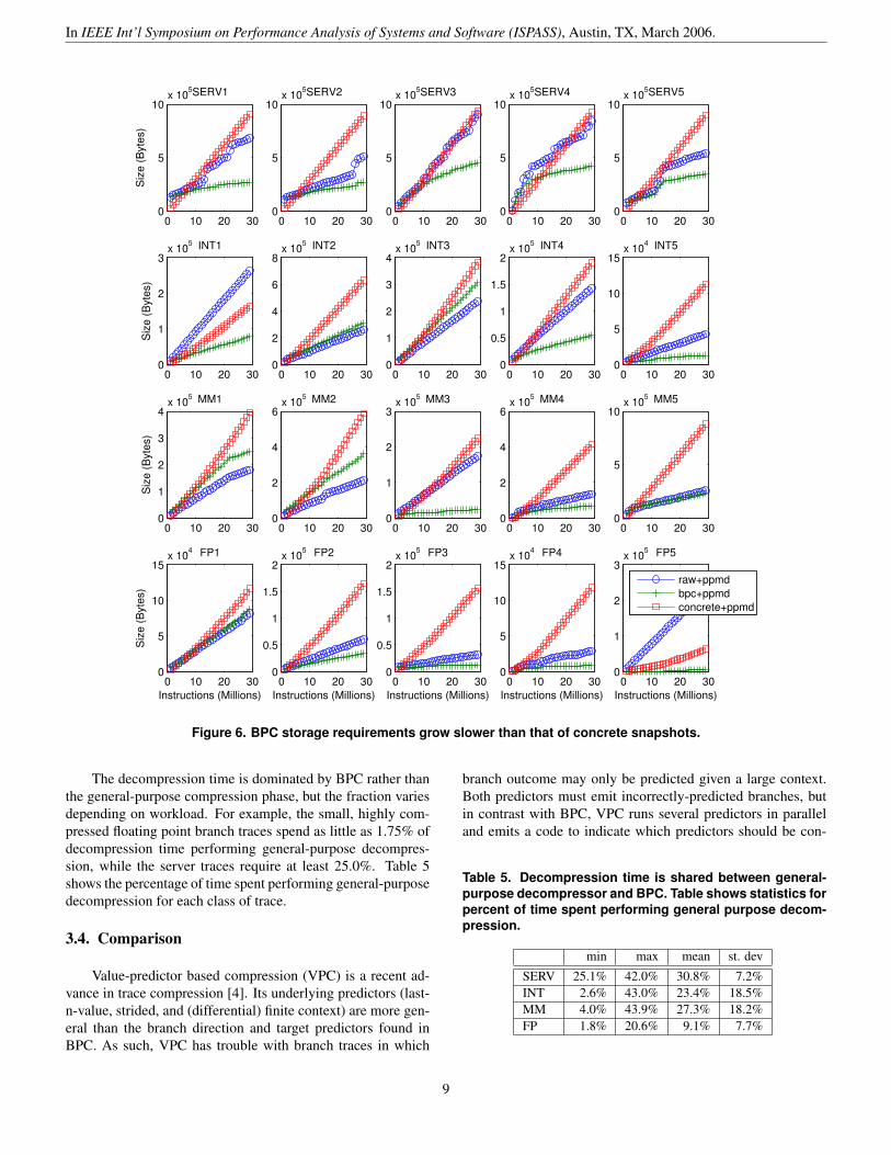
3.2. Scaling

How can we be certain that the compression ratios ob-served on this short trace will carry through an entire programexecution? We extrapolate from the data shown in Figure 6which shows how storage requirements scale over time. Sincea single compressed trace suffices to represent all branches inthe program, we report the current size of the compressed traceat every 1M instructions. For the concrete snapshots, we reportthe cumulative snapshot size at the given instant. Note that Fig-ure 4 is merely the final data point of Figure 6 divided by thenumber of branches observed and multiplied by 8 bits.

As the program begins, the concrete predictors are largelyunused and the easily compressed. Thus, their total size isless than a compressed trace. As the program progresses, theconcrete predictors are harder to compress and make a dra-matic contribution to the overall snapshot size. For all work-loads, trace compression scales better than storing concretepredictors. In 15/20 cases, BPC compression fares better thanPPMd compression of a raw branch trace; in two other cases(INT2 and FP1) it is competitive or nearly equal, leaving threecases (MM1, MM2, and INT3) in which PPMd outperforms

7


BPC+PPMd. The server benchmarks present an interestingchallenge to the compression techniques. In general, theseworkloads contain branches which are harder to predict andphase changes which are more pronounced. BPC, with itshardware-style internal branch predictors, is more suited toquick adaptation than PPMd which uses more generic predic-tion. When returning to a phase, BPC’s large tables and longhistory allow better prediction than PPMd, which must adjustits probability models as new inputs are seen; when old inputsreturn, the model’s representation of old data is less optimal.

The figure shows trends developing in the early stages ofexecution that should continue throughout the program. A tracecompressed with BPC will grow slowly as new static branchesappear, but reoccurrence of old branches will be easily pre-dicted and concisely expressed (unless purged from the model).Storage of concrete snapshots grows with mnP as discussed inSection 3.1.

3.3. Timing

We have shown the storage advantages of trace-basedreconstruction versus snapshot-based reconstruction, but wemust show that the time required to compress and decompressthe data does not outweigh the space savings. In the case ofBPC or BPC+general purpose compression, the cost is negli-gible. BPC requires simple predictors and tables which addslittle time to functional simulation. The second-stage, general-purpose compressors (gzip, bzip2, and PPMd) are highly op-timized and use fixed-size tables, so they remain fast through-out the compression process. Furthermore, compression is per-formed once, so the creation time of a microarchitectural snap-shot can be amortized over many detailed simulations. We nolonger have to guess likely configurations, fix a maximum size,or regenerate a snapshot to reflect a microarchitectural change.

Decompression speed is more important. We presume aparallel methodology in which independent snapshots are pro-duced and used to warm up state for detailed samples on mul-tiple machines. In such a situation, runtime is limited by thetime to warm the final sample in program order. When work-ing with a non-random-access compressed trace such as BPC,the warming for the final sample in the program requires ex-amining every branch in the trace. While this is much slowerthan directly loading a snapshot of microarchitectural state, itis much faster than functional simulation. Intuitively, warmingvia branch trace decompression can be faster than functionalsimulation: not only are there many fewer branches than totalinstructions, but for each branch, only a few table updates arerequired rather than an entire decode and execute phase. Wehave traded some speed for lots of flexibility while remainingseveral times faster than traditional functional branch predictorwarming. On average, BPC adds 48 seconds for every billioninstructions in the program on our test platform.

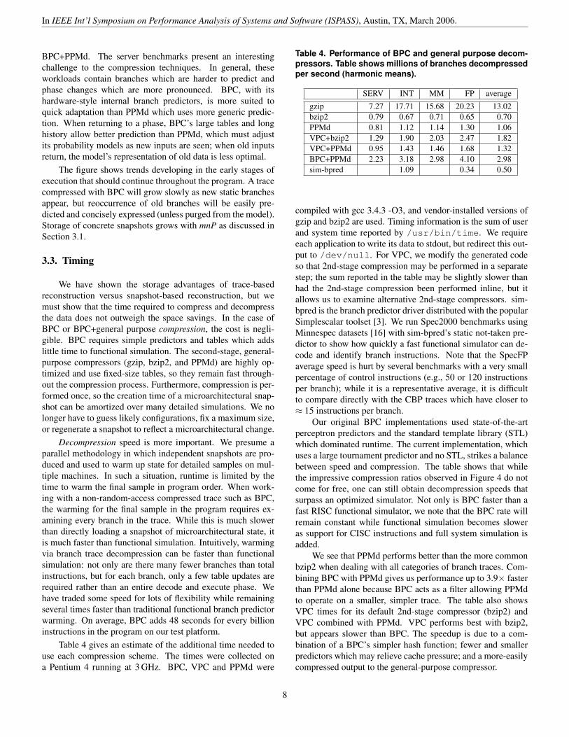
Table 4 gives an estimate of the additional time needed touse each compression scheme. The times were collected ona Pentium 4 running at 3 GHz. BPC, VPC and PPMd were

Table 4. Performance of BPC and general purpose decom-pressors. Table shows millions of branches decompressedper second (harmonic means).

SERV INT MM FP average

gzip 7.27 17.71 15.68 20.23 13.02bzip2 0.79 0.67 0.71 0.65 0.70PPMd 0.81 1.12 1.14 1.30 1.06VPC+bzip2 1.29 1.90 2.03 2.47 1.82VPC+PPMd 0.95 1.43 1.46 1.68 1.32BPC+PPMd 2.23 3.18 2.98 4.10 2.98sim-bpred 1.09 0.34 0.50

compiled with gcc 3.4.3 -O3, and vendor-installed versions ofgzip and bzip2 are used. Timing information is the sum of userand system time reported by /usr/bin/time. We requireeach application to write its data to stdout, but redirect this out-put to /dev/null. For VPC, we modify the generated codeso that 2nd-stage compression may be performed in a separatestep; the sum reported in the table may be slightly slower thanhad the 2nd-stage compression been performed inline, but itallows us to examine alternative 2nd-stage compressors. sim-bpred is the branch predictor driver distributed with the popularSimplescalar toolset [3]. We run Spec2000 benchmarks usingMinnespec datasets [16] with sim-bpred’s static not-taken pre-dictor to show how quickly a fast functional simulator can de-code and identify branch instructions. Note that the SpecFPaverage speed is hurt by several benchmarks with a very smallpercentage of control instructions (e.g., 50 or 120 instructionsper branch); while it is a representative average, it is difficultto compare directly with the CBP traces which have closer to≈ 15 instructions per branch.

Our original BPC implementations used state-of-the-artperceptron predictors and the standard template library (STL)which dominated runtime. The current implementation, whichuses a large tournament predictor and no STL, strikes a balancebetween speed and compression. The table shows that whilethe impressive compression ratios observed in Figure 4 do notcome for free, one can still obtain decompression speeds thatsurpass an optimized simulator. Not only is BPC faster than afast RISC functional simulator, we note that the BPC rate willremain constant while functional simulation becomes sloweras support for CISC instructions and full system simulation isadded.

We see that PPMd performs better than the more commonbzip2 when dealing with all categories of branch traces. Com-bining BPC with PPMd gives us performance up to 3.9× fasterthan PPMd alone because BPC acts as a filter allowing PPMdto operate on a smaller, simpler trace. The table also showsVPC times for its default 2nd-stage compressor (bzip2) andVPC combined with PPMd. VPC performs best with bzip2,but appears slower than BPC. The speedup is due to a com-bination of a BPC’s simpler hash function; fewer and smallerpredictors which may relieve cache pressure; and a more-easilycompressed output to the general-purpose compressor.

8


0 10 20 300

5

10x 105SERV1

Size

(Byt

es)

0 10 20 300

5

10x 105SERV2

0 10 20 300

5

10x 105SERV3

0 10 20 300

5

10x 105SERV4

0 10 20 300

5

10x 105SERV5

0 10 20 300

1

2

3x 105 INT1

Size

(Byt

es)

0 10 20 300

2

4

6

8x 105 INT2

0 10 20 300

1

2

3

4x 105 INT3

0 10 20 300

0.5

1

1.5

2x 105 INT4

0 10 20 300

5

10

15x 104 INT5

0 10 20 300

1

2

3

4x 105 MM1

Size

(Byt

es)

0 10 20 300

2

4

6x 105 MM2

0 10 20 300

1

2

3x 105 MM3

0 10 20 300

2

4

6x 105 MM4

0 10 20 300

5

10x 105 MM5

0 10 20 300

5

10

15x 104 FP1

Instructions (Millions)

Size

(Byt

es)

0 10 20 300

0.5

1

1.5

2x 105 FP2

Instructions (Millions)0 10 20 30

0

0.5

1

1.5

2x 105 FP3


0

5

10

15x 104 FP4


0

1

2

3x 105 FP5

Instructions (Millions)

raw+ppmdbpc+ppmdconcrete+ppmd

Figure 6. BPC storage requirements grow slower than that of concrete snapshots.

The decompression time is dominated by BPC rather thanthe general-purpose compression phase, but the fraction variesdepending on workload. For example, the small, highly com-pressed floating point branch traces spend as little as 1.75% ofdecompression time performing general-purpose decompres-sion, while the server traces require at least 25.0%. Table 5shows the percentage of time spent performing general-purposedecompression for each class of trace.

3.4. Comparison

Value-predictor based compression (VPC) is a recent ad-vance in trace compression [4]. Its underlying predictors (last-n-value, strided, and (differential) finite context) are more gen-eral than the branch direction and target predictors found inBPC. As such, VPC has trouble with branch traces in which

branch outcome may only be predicted given a large context.Both predictors must emit incorrectly-predicted branches, butin contrast with BPC, VPC runs several predictors in paralleland emits a code to indicate which predictors should be con-

Table 5. Decompression time is shared between general-purpose decompressor and BPC. Table shows statistics forpercent of time spent performing general purpose decom-pression.

min max mean st. dev

SERV 25.1% 42.0% 30.8% 7.2%INT 2.6% 43.0% 23.4% 18.5%MM 4.0% 43.9% 27.3% 18.2%FP 1.8% 20.6% 9.1% 7.7%

9


sulted for each record. When an internal predictor cannot beused, the unpredictable portion of the record is output. Sep-arate output streams are used corresponding to each internalpredictor.

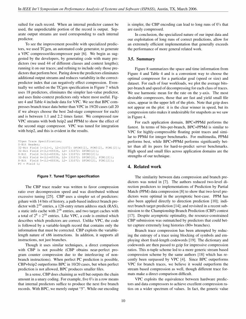
To see the improvement possible with specialized predic-tors, we used TCgen, an automated code generator, to generatea VPC compressor/decompressor pair [6]. We begin as sug-gested by the developers, by generating code with many pre-dictors (we used 44 of different classes and context lengths);running it on our traces; and refining to include only those pre-dictors that perform best. Paring down the predictors eliminatesadditional output streams and reduces variability in the correct-predictor index that can negatively effect compression. Even-tually we settled on the TCgen specification in Figure 7 whichuses 18 predictors, eliminates the simpler last-value predictor,and uses finite-context predictors only where most useful. Fig-ure 4 and Table 4 include data for VPC. We see that BPC com-presses branch trace data better than VPC in 19/20 cases (all 20if we always choose the best 2nd-stage compressor for each)and is between 1.1 and 2.2 times faster. We compressed rawVPC streams with both bzip2 and PPMd to show the effect ofthe second stage compressor. VPC was tuned for integrationwith bzip2, and this is evident in the results.

TCgen Trace Specification;0-Bit Header;32-Bit Field 1={L1=1, L2=131072: DFCM3[2], FCM3[2], FCM1[2]};32-Bit Field 2={L1=65536, L2= 131072: DFCM3[2]};8-Bit Field 3={L1=65536, L2= 131072: DFCM3[2]};32-Bit Field 4={L1=65536, L2= 131072: DFCM3[2], FCM1[2]};8-Bit Field 5={L1=65536, L2= 131072: DFCM3[2], FCM1[2]};PC = Field 1;

Figure 7. Tuned TCgen specification

The CBP trace reader was written to favor compressionratio over decompression speed and was distributed withoutexcessive tuning [25]. CBP uses a simpler set of predictors:gshare with 14 bits of history, a path-based indirect branch pre-dictor with 210 entries, a 128-entry return address stack (RAS),a static info cache with 218 entries, and two target caches witha total of 28 + 216 entries. Like VPC, a code is emitted whichdescribes which predictors are correct. Unlike VPC, the codeis followed by a variable-length record that contains only theinformation that must be corrected. CBP exploits the variable-length nature of x86 instructions. In addition, it supports allinstructions, not just branches.

Though it uses similar techniques, a direct comparisonwith CBP is not possible (CBP obtains near-perfect pro-gram counter compression due to the interleaving of non-branch instructions). When perfect PC prediction is possible,CBP+bzip2 outperforms BPC in 10/20 cases, but when perfectprediction is not allowed, BPC produces smaller files.

In a sense, CBP does chaining as well but outputs the chainamount in a unary coding. For example, five 0’s in a row meansthat internal predictors suffice to produce the next five branchrecords. With BPC, we merely output “5”. While our encoding

is simpler, the CBP encoding can lead to long runs of 0’s thatare easily compressed.

In conclusion, the specialized nature of our input data andour exploitation of long runs of correct predictions, allow foran extremely efficient implementation that generally exceedsthe performance of more general related work.

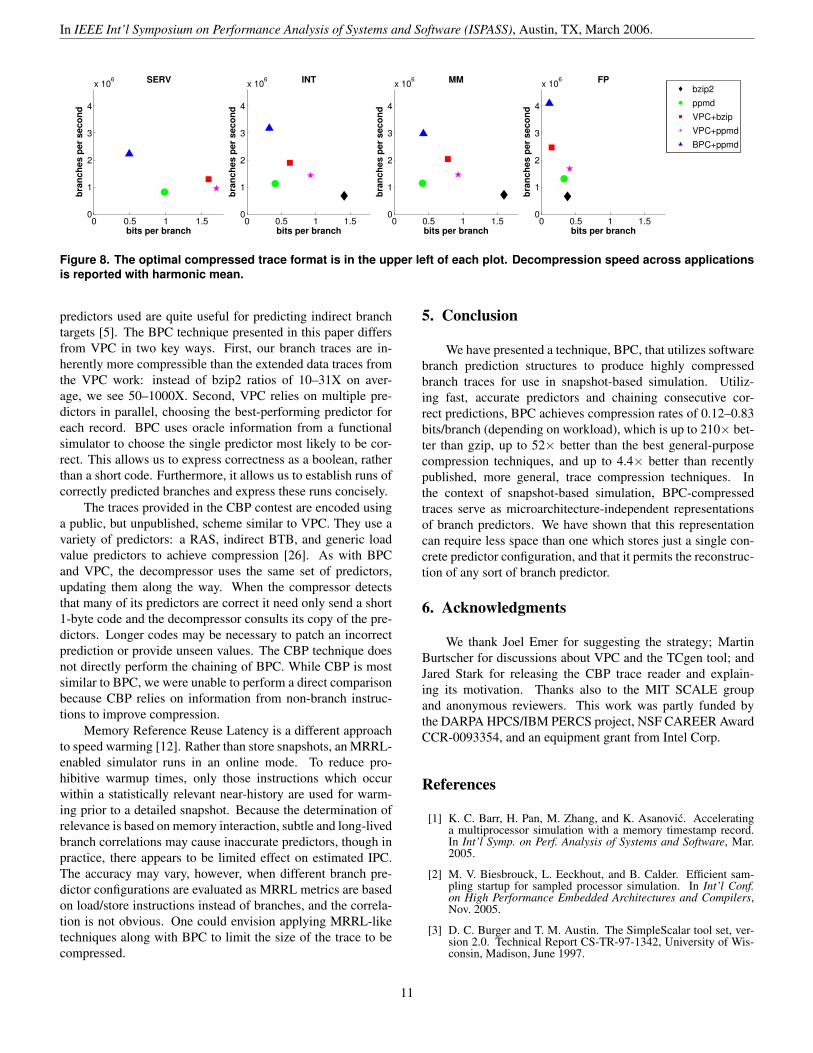
3.5. Summary

Figure 8 summarizes the space and time information fromFigure 4 and Table 4 and is a convenient way to choose theoptimal compressor for a particular goal (speed or size) anddataset. For each of four workloads, we plot the average bits-per-branch and speed of decompressing for each class of traces.We use harmonic mean for the rate on the y-axis. The mostdesirable compressors, those that are fast and yield small filesizes, appear in the upper left of the plots. Note that gzip doesnot appear on the plot: it is the clear winner in speed, but itscompression ratio makes it undesirable for snapshots as we sawin Figure 4.

For each application domain, BPC+PPMd performs thefastest. In terms of bits-per-branch, BPC+PPMd is similar toVPC for highly-compressible floating point traces and simi-lar to PPMd for integer benchmarks. For multimedia, PPMdperforms best, while BPC+PPMd performs significantly bet-ter than all its peers for hard-to-predict server benchmarks.High speed and small files across application domains are thestrengths of our technique.

4. Related work

The similarity between data compression and branch pre-dictors was noted in [7]. The authors reduced two-level di-rection predictors to implementations of Prediction by PartialMatch (PPM) data compression [8] to show that two-level pre-dictors were optimal in the asymptotic best-case. PPM hasalso been applied directly to direction prediction [10]; indi-rect branch target prediction [14]; and revisited in a recent sub-mission to the Championship Branch Prediction (CBP) contest[17]. Despite asymptotic optimality, the resource-constrainedCBP submission was outmatched by predictors that could bet-ter capture extremely long histories (80+ branches).

Branch trace compression has been attempted by reduc-ing the entropy of a trace using blocking of symbols and em-ploying short fixed-length codewords [19]. The dictionary andcodewords are then passed to gzip for impressive compressionratios. This n-tuple scheme led to a more generic stream basedcompression scheme by the same authors [18] which has re-cently been surpassed by VPC [4]. Since BPC outperformsVPC for branch traces, we believe it would outperform thestream based compression as well, though different trace for-mats make a direct comparison difficult.

VPC exploits the equivalence between hardware predic-tors and data compressors to achieve excellent compression ra-tios on a wider spectrum of values. In fact, the generic value

10


0 0.5 1 1.50

1

2

3

4

x 106 SERV

bits per branch

bran

ches

per

sec

ond

0 0.5 1 1.50

1

2

3

4

x 106 INT

bits per branchbr

anch

es p

er s

econ

d0 0.5 1 1.5

0

1

2

3

4

x 106 MM

bits per branch

bran

ches

per

sec

ond

0 0.5 1 1.50

1

2

3

4

x 106 FP

bits per branch

bran

ches

per

sec

ond

bzip2ppmdVPC+bzipVPC+ppmdBPC+ppmd

Figure 8. The optimal compressed trace format is in the upper left of each plot. Decompression speed across applicationsis reported with harmonic mean.

predictors used are quite useful for predicting indirect branchtargets [5]. The BPC technique presented in this paper differsfrom VPC in two key ways. First, our branch traces are in-herently more compressible than the extended data traces fromthe VPC work: instead of bzip2 ratios of 10–31X on aver-age, we see 50–1000X. Second, VPC relies on multiple pre-dictors in parallel, choosing the best-performing predictor foreach record. BPC uses oracle information from a functionalsimulator to choose the single predictor most likely to be cor-rect. This allows us to express correctness as a boolean, ratherthan a short code. Furthermore, it allows us to establish runs ofcorrectly predicted branches and express these runs concisely.

The traces provided in the CBP contest are encoded usinga public, but unpublished, scheme similar to VPC. They use avariety of predictors: a RAS, indirect BTB, and generic loadvalue predictors to achieve compression [26]. As with BPCand VPC, the decompressor uses the same set of predictors,updating them along the way. When the compressor detectsthat many of its predictors are correct it need only send a short1-byte code and the decompressor consults its copy of the pre-dictors. Longer codes may be necessary to patch an incorrectprediction or provide unseen values. The CBP technique doesnot directly perform the chaining of BPC. While CBP is mostsimilar to BPC, we were unable to perform a direct comparisonbecause CBP relies on information from non-branch instruc-tions to improve compression.

Memory Reference Reuse Latency is a different approachto speed warming [12]. Rather than store snapshots, an MRRL-enabled simulator runs in an online mode. To reduce pro-hibitive warmup times, only those instructions which occurwithin a statistically relevant near-history are used for warm-ing prior to a detailed snapshot. Because the determination ofrelevance is based on memory interaction, subtle and long-livedbranch correlations may cause inaccurate predictors, though inpractice, there appears to be limited effect on estimated IPC.The accuracy may vary, however, when different branch pre-dictor configurations are evaluated as MRRL metrics are basedon load/store instructions instead of branches, and the correla-tion is not obvious. One could envision applying MRRL-liketechniques along with BPC to limit the size of the trace to becompressed.

5. Conclusion

We have presented a technique, BPC, that utilizes softwarebranch prediction structures to produce highly compressedbranch traces for use in snapshot-based simulation. Utiliz-ing fast, accurate predictors and chaining consecutive cor-rect predictions, BPC achieves compression rates of 0.12–0.83bits/branch (depending on workload), which is up to 210× bet-ter than gzip, up to 52× better than the best general-purposecompression techniques, and up to 4.4× better than recentlypublished, more general, trace compression techniques. Inthe context of snapshot-based simulation, BPC-compressedtraces serve as microarchitecture-independent representationsof branch predictors. We have shown that this representationcan require less space than one which stores just a single con-crete predictor configuration, and that it permits the reconstruc-tion of any sort of branch predictor.

6. Acknowledgments

We thank Joel Emer for suggesting the strategy; MartinBurtscher for discussions about VPC and the TCgen tool; andJared Stark for releasing the CBP trace reader and explain-ing its motivation. Thanks also to the MIT SCALE groupand anonymous reviewers. This work was partly funded bythe DARPA HPCS/IBM PERCS project, NSF CAREER AwardCCR-0093354, and an equipment grant from Intel Corp.

References

[1] K. C. Barr, H. Pan, M. Zhang, and K. Asanovic. Acceleratinga multiprocessor simulation with a memory timestamp record.In Int’l Symp. on Perf. Analysis of Systems and Software, Mar.2005.

[2] M. V. Biesbrouck, L. Eeckhout, and B. Calder. Efficient sam-pling startup for sampled processor simulation. In Int’l Conf.on High Performance Embedded Architectures and Compilers,Nov. 2005.

[3] D. C. Burger and T. M. Austin. The SimpleScalar tool set, ver-sion 2.0. Technical Report CS-TR-97-1342, University of Wis-consin, Madison, June 1997.

11


[4] M. Burtscher, I. Ganusov, S. J. Jackson, J. Ke, P. Ratanaworab-han, and N. B. Sam. The VPC trace-compression algorithms.IEEE Trans. on Computers, 54(11), Nov. 2005.

[5] M. Burtscher and M. Jeeradit. Compressing extended programtraces using value predictors. In Int’l Conf. on Parallel Architec-tures and Compilation Techniques, Sept. 2003.

[6] M. Burtscher and N. B. Sam. Automatic generation of high-performance trace compressors. In Int’l Symp. on Code Genera-tion and Optimization, Mar. 2005.

[7] I.-C. K. Chen, J. T. Coffey, and T. N. Mudge. Analysis of branchprediction via data compression. In Int’l Conf. on ArchitecturalSupport for Prog. Languages and Operating Systems, 1996.

[8] J. G. Cleary and I. H. Witten. Data compression using adaptivecoding and partial string matching. IEEE Trans. on Communi-cations, 32(4), Apr. 1984.

[9] K. Driesen and U. Holzle. The cascaded predictor: Economicaland adaptive branch target prediction. In Int’l Symp. on Microar-chitecture, Dec. 1998.

[10] E. Federovsk, M. Feder, and S. Weiss. Branch prediction basedon universal data compression algorithms. In Int’l Symp. onComputer Architecture, June 1998.

[11] J. Gailly and M. Adler. gzip 1.3.3. http://www.gzip.org,2002.

[12] J. W. Haskins and K. Skadron. Memory reference reuse latency:Accelerated warmup for sampled microarchitecture. In Int’lSymp. on Perf. Analysis of Systems and Software, Mar. 2003.

[13] M. D. Hill and A. J. Smith. Evaluating associativity in CPUcaches. IEEE Trans. on Computers, C-38(12), Dec 1989.

[14] J. Kalamatianos and D. R. Kaeli. Predicting indirect branches viadata compression. In Int’l Symp. on Microarchitecture, 1998.

[15] R. Kessler. The Alpha 21264 microprocessor. IEEE Micro,19(2), March-April 1999.

[16] A. KleinOsowski and D. J. Lilja. MinneSPEC: A new SPECbenchmark workload for simulation-based computer architec-ture research. Computer Architecture Letters, vol. 1, June 2002.

[17] P. Michaud. A PPM-like, tag-based predictor. In ChampionshipBranch Prediction Competition, 2004.

[18] A. Milenkovic and M. Milenkovic. Exploiting streams in in-struction and data address trace compression. In IEEE Workshopon Workload Characterization, Oct. 2003.

[19] A. Milenkovic, M. Milenkovic, and J. Kulick. N-tuple com-pression: A novel method for compression of branch instructiontraces. In Int’l Conf. on Parallel and Distributed Computing Sys-tems, Aug 2003.

[20] M. Milenkovic, A. Milenkovic, and J. Kulick. Demystifying in-tel branch predictors. In Workshop on Duplicating, Deconstruct-ing and Debunking, May 2002.

[21] E. Perelman, G. Hamerly, and B. Calder. Picking statisticallyvalid and early simulation points. In Int’l Conf. on Parallel Ar-chitectures and Compilation Techniques, Sep 2003.

[22] J. C. Ram Srinivasan and S. Cooper. Fast, accurate microarchi-tecture simulation using statistical phase detection. In Int’l Symp.on Perf. Analysis of Systems and Software, Mar 2005.

[23] J. Seward. bzip2 1.0.2. http://www.bzip.org, 2001.

[24] D. Shkarin. PPM: one step to practicality. In Data CompressionConf., 2002.

[25] J. W. Stark. personal communication via email, Oct. 2005.

[26] J. W. Stark and C. Wilkerson et al. The 1st JILP championshipbranch prediction competition. In Workshop at MICRO-37 andJournal of ILP, Jan. 2005. http://www.jilp.org/cbp/.

[27] R. A. Sugummar. Multi-Configuration Simulation Algorithmsfor the Evaluation of Computer Architecute Designs. PhD thesis,University of Michigan, Aug. 1993. Technical Report CSE-TR-173-93.

[28] J. G. Thompson. Efficient analysis of caching systems. PhDthesis, University of California at Berkeley, 1987.

[29] T. F. Wenisch, R. E. Wunderlich, B. Falsafi, and J. C. Hoe.Turbosmarts: accurate microarchitecture simulation sampling inminutes. SIGMETRICS Perform. Eval. Rev., 33(1), 2005.

[30] R. Wunderlich et al. SMARTS: Accelerating microarchitecturesimulation via rigorous statistical sampling. In Int’l Symp. onComputer Architecture, June 2003.

12

Documents

Branch trace compression for snapshot-based …krste/papers/bpred-ispass06.pdfBranch Trace Compression for Snapshot-Based Simulation ... a matching software branch predictor to help