A robust framework for soft tissue simulations with application to modeling brain tumor mass

effect in 3D MR images

This article has been downloaded from IOPscience. Please scroll down to see the full text article.

2007 Phys. Med. Biol. 52 6893

(http://iopscience.iop.org/0031-9155/52/23/008)

Download details:

IP Address: 165.123.243.100

The article was downloaded on 30/03/2011 at 19:16

Please note that terms and conditions apply.

View the table of contents for this issue, or go to the journal homepage for more

Home Search Collections Journals About Contact us My IOPscience

IOP PUBLISHING PHYSICS IN MEDICINE AND BIOLOGY

Phys. Med. Biol. 52 (2007) 6893–6908 doi:10.1088/0031-9155/52/23/008

A robust framework for soft tissue simulations withapplication to modeling brain tumor mass effect in 3DMR images

Cosmina Hogea1, George Biros2, Feby Abraham3 andChristos Davatzikos1

1 Section of Biomedical Image Analysis, Department of Radiology, University of Pennsylvania,Philadelphia PA 19104, USA2 Department of Mechanical Engineering and Applied Mechanics, University of Pennsylvania,Philadelphia PA 19104, USA3 GlaxoSmithKline, Scientific Computing and Mathematical Modeling Group, King of Prussia,PA, USA

E-mail: hogeac@uphs.upenn.edu

Received 29 June 2007, in final form 14 October 2007Published 8 November 2007Online at stacks.iop.org/PMB/52/6893

AbstractWe present a framework for black-box and flexible simulation of soft tissuedeformation for medical imaging and surgical planning applications. Ourmain motivation in the present work is to develop robust algorithms that allowbatch processing for registration of brains with tumors to statistical atlases ofnormal brains and construction of brain tumor atlases. We describe a fullyEulerian formulation able to handle large deformations effortlessly, with alevel-set-based approach for evolving fronts. We use a regular grid—fictitiousdomain method approach, in which we approximate coefficient discontinuities,distributed forces and boundary conditions. This approach circumvents theneed for unstructured mesh generation, which is often a bottleneck in themodeling and simulation pipeline. Our framework employs penalty approachesto impose boundary conditions and uses a matrix-free implementation coupledwith a multigrid-accelerated Krylov solver. The overall scheme results in ascalable method with minimal storage requirements and optimal algorithmiccomplexity. We illustrate the potential of our framework to simulate realisticbrain tumor mass effects at reduced computational cost, for aiding theregistration process towards the construction of brain tumor atlases.

1. Introduction

The biomechanical modeling of soft tissue deformation has been receiving increasing attentionin the biomedical imaging community. Such deformations are commonly caused by breathing,

0031-9155/07/236893+16$30.00 © 2007 IOP Publishing Ltd Printed in the UK 6893

6894 C Hogea et al

tumor growth, injuries, or surgical procedures. Their modeling and estimation are importantfor registration motion tracking, construction of statistical atlases and surgical planning.There is an extensive amount of algorithms for soft tissue deformation modeling. Herewe are interested in simulation frameworks for medical imaging, particularly in the contextof reducing the computational time and cost. Examples are Dawant et al (1999), Ferrantet al (2001), Miga et al (1998), Warfield et al (2002, 2003) and Cotin et al (1999).Biomechanical simulations of tissue deformations usually start with obtaining a segmentationof the target geometry from a medical image which is then used to reconstruct a representationof the target geometry’s boundary surface. The surface is interfaced to an unstructuredgrid generation code (e.g., tetrahedral meshing, Mohamed and Davatzikos (2005)). Thereexist, however, multiple challenges in boundary resolving mesh generation techniques. First,there are no robust unstructured mesh generation algorithms with guaranteed approximationproperties (Shewchuk 2000). Unstructured meshes create a bottleneck in the presence oflarge deformation (or more generally problems with dynamic interfaces, e.g., evolving tumor–brain interfaces); under large strain fields, the mesh quality deteriorates and requires frequentoffline remeshing (Mohamed and Davatzikos 2004). Second, once a discretization has beenobtained the construction of efficient solvers for the resulting algebraic system of equationsis difficult. The work for sparse direct (e.g. LU factorization) or iterative (e.g. Krylov) doesnot scale with the number of unknowns. Most importantly, soft tissue simulations are oftenplagued by imprecise geometry information, unknown constitutive laws, boundary conditionsand distributed forces. Under such circumstances, making an effort to accurately representgeometry seems rather unnecessary. For these reasons, many researchers in the medicalimaging community use regular grids—a rather natural choice since the input data are givenon such a grid. Material properties can be assigned based on the images or their segmentationand a fictitious domain method (Shah et al 1995) avoids the geometric constrains. Regulargrids however, pose significant drawbacks: (1) it is difficult to apply boundary conditionsinside the domain without effecting the condition number of the resulting operator, (2) strongmaterial contrasts cause severe ill-conditioning and slow down the solvers and (3) the largeproblem size due to lack of adaptivity.

In this paper we propose a general regular grid methodology for arbitrary geometriesthat circumvents these difficulties: it allows for fast solutions, high material contrasts, avariety of different boundary conditions and distributed forces in arbitrary regions inside ofthe domain. The target domain, consisting of a possibly inhomogeneous, anisotropic, andnonlinear material is embedded on a larger computational cubic domain (box). The materialproperties and distributed forces are chosen so that the imposed boundary conditions on thetrue boundary are approximated adequately. An Eulerian formulation is employed to capturelarge deformations, with a level-set-based approach for evolving fronts.

Our main motivation in the present work is to develop algorithms that can be used in arobust, black-box fashion for registration of brains with tumors to statistical atlases of normalbrains. Clinical applications include morphometry, surgical planning and post-operativeanalysis. The proposed framework results in a converging (but low-order) method thatcircumvents the need for mesh generation and has the ability to simulate large deformations.We use a matrix-free implementation where only the material properties and work vectors arestored; we combine it with a geometric full V-cycle multigrid approach. In instances wherecomputational speed/efficiency prevails the need for high numerical accuracy, this seems anoptimal and promising alternative. We presently employ it successfully for simulating realisticlarge brain tumor mass effects, with the ultimate purpose of aiding the registration processtoward the construction of brain tumor atlases.

Brain tumor mass effect in 3D MR images: a robust simulation framework 6895

2. Methods

In this section, we present a fully Eulerian framework for simulating soft tissue deformationin conjunction with medical imaging, with emphasis on brain tissue deformation followingtumor growth (mass effect). Our main general goals are (1) to be able to simulate largedeformations robustly, without meshing/remeshing issues; (2) to handle general irregulargeometries and boundary conditions fast and inexpensive—even if at the cost of reducedapproximation accuracy (justified from inherent uncertainties in the model.)

2.1. Eulerian formulation for large deformations

For the sake of generality, let us start with an abstract general formulation for biomechanicalsimulations of soft tissue deformation. Consider a deforming elastic body occupying a boundedregion in space ω (see figure 1; in general, ω can be arbitrarily shaped and can include anynumber of inhomogeneities and/or internal interfaces). In contrast with standard Lagrangianor arbitrary Lagrangian–Eulerian techniques, we resort to a formulation which is rather unusualfor solids since it is written exclusively in an Eulerian frame of reference. The motion of adeformable solid is described by

ρv = ∇ · T + b, momentum

T = T(F, F), constitutive

F = ∇vF, u = v, kinematics (1)

Cu + Tn = q, on γ × (0, T ), boundary conditions

m = 0, transport.

Here v is the velocity field and ˙ is the material time derivative operator: for a scalar, vectoror tensor field z, the material time derivative (given an underlying motion described bythe velocity v) is z := ∂z

∂t+ (∇z)v. The spatial differential operators are with respect to

x = χ(p, t), regarded as the place occupied by the particle p at instant t, where χ representsthe particle motion. u is the displacement field, T is the Cauchy stress tensor and T denotes theconstitutive law depending on the deformation tensor F = I + ∇u and its time derivative F; nis the outward normal defined on the boundary of ω, C is a given linear algebraic operator thatencapsulates mixed, Neumann and Dirichlet boundary conditions; q is given boundary data;b represents distributed forces (like gravity) or forces from internal interfaces: for example,in the schematical representation in figure 1, there may be a surface force on the boundaryγ2 of the internal domain ω2. Finally m represents material properties and interfaces that areadvected with the motion of the material. In general, the distributed forces and the constitutivelaw will depend on m, which makes the above system of equations strongly coupled. Ourgeneral numerical solution scheme is based on a semi-implicit approach, in which we advectthe material properties explicitly, and then we solve for the momentum implicitly. The systemof equations (1) is augmented with initial conditions for u, v, F, m.

This formulation is general and can be used with any constitutive law. For simplicity, herewe will be focusing on the case of a Maxwell-like viscoelastic solid for which the externalloads are applied in a time-piecewise fashion so that there is an instantaneous linear elasticresponse followed by a stress and elastic strain relaxation. In this case, equations (1) become

∇ · T + b = 0, momentum

T = (λ∇ · u)I + µ(∇u + ∇uT ), constitutive

Cu + Tn = q, on γ × (0, T ), boundary conditions (2)

6896 C Hogea et al

ω1

ω2

ωγ

ω1

ω2

ωγΩ

Γ

sω1

ω2

ωγΩ

Γ

stiff

sω1

ω2

ωγΩ

Γ

soft

δσ

ω1

ω2

ωγΩ

Γ

(a) (b) (c) (d) (e)

Figure 1. Regular grid simulations for irregular geometries: (a) input domain ω withinhomogeneities (ω1, ω2); (b) embedding ω in a larger fictitious domain with boundary ;(c) approximating Dirichlet conditions with a stiff material for \ω; (d) approximating Neumannconditions σ with a soft material; (e) regular grid discretization. For the brain tumor simulations,the cubic domain is identical to the 3D MR image.

(This figure is in colour only in the electronic version)

v = ∂u∂t

, kinematics

m = 0, transport,

where m = λ,µ, ϕ are quantities advected with the velocity v of the underlying material.The reduced expression of the velocity field v holds in the linearized theory. Here, λ and µ arethe inhomogeneous (location varying) Lame parameters (related to Young’s modulus E andPoisson’s ratio ν), while ϕ is the level-set function associated with an interface that we wouldlike to track. More specific details for our particular application to simulation of mass effectinduced by growing brain tumors follow in section 2.4.

2.2. Regular grid solver

To solve the static linear elasticity problem, we use trilinear finite elements to approximatethe displacements in the momentum equation, and piecewise constant functions for λ, ν. Oneimportant issue is the accurate integration of the elements that overlap in the inhomogeneitytransition, since jumps in the material properties can cause large numerical errors. Here,for simplicity, and in accordance with medical imaging practice, we use voxelized materialproperties. The Poisson ratio ν(x) varies between zero for a perfectly compressible materialand 0.5 for a fully incompressible material. Most soft tissues can be considered as nearlyincompressible. (As ν approaches 0.5, commonly used displacement-based finite elementimplementations suffer from the so-called locking effect. We use underintegration for the∇ · u term in the stress; see Hughes (1987) for details.)

2.2.1. Imposing boundary conditions. Case (c) in figure 1 illustrates zero Dirichlet boundaryconditions, which can be approximated by either Lagrange multipliers or a simpler penaltyformulation (Babuška 1973). The latter corresponds to having a very stiff material surroundingthe target domain. The nonzero case can be treated by linearity: we construct a smooth functionU such that U = g on γ , where g are the specified boundary conditions. We represent thesolution of Lu = f as u = U + w, and we solve for Lw = f −LU with homogeneous Dirichletconditions (L is the linear elasticity operator); U is constructed using a triangulation, or alevel-set representation of the boundary.

For the general Neumann or mixed boundary conditions, we consider a different approach,based on the fictitious domain method (Glowinski et al 1996, Angot et al 2005). For simplicityand concision, we illustrate it here on a model Poisson problem, but the exact same approach

Brain tumor mass effect in 3D MR images: a robust simulation framework 6897

extends to the elasticity problem; all the results presented here in section 3 are for the linearelasticity case.

Consider the following model problem:

−∇ · (µ∇u) = 0 in ω, cu +∂u

∂n= q on γ.

Its weak form can be written as∫ω

µ∇u · ∇v dω +∫

γ

c uv dγ =∫

γ

qv dγ, ∀ v.

We can extend the weak form to a larger domain by introducing an approximation of thecharacteristic function for the domain ω (its value is one inside ω and zero outside):∫

(ε + χω)µ∇u · ∇v d +∫

γ

c uv dγ =∫

γ

qv dγ, ∀ v.

Neumann conditions can be imposed by using a soft material (case (d) in figure 1), usedto approximate χω. Dirichlet conditions can be imposed by selecting a very large parameter c.For linear elasticity, mixed conditions (say Neumann in the tangential direction, and Dirichletin the normal) can be imposed by choosing an appropriate function c.

The convergence rates are suboptimal (compared to the convergence rate expected by theinterpolation power of the underlying FEM basis) for the jumps in the material properties,whereas the boundary conditions are satisfied only approximately—for the Neumann andDirichlet cases (Glowinski et al 1996).

2.2.2. Choice of penalty parameter. Related theory can be found in Babuška (1973),Glowinski et al (1996), Angot et al (2005), DelPino and Pironneau (2003). The generalguidelines are to use O(1/h) for stiff materials (Dirichlet conditions) and O(h) for softmaterials (Neumann conditions), where h is the mesh size used for spatial discretization. Theresults are not sensitive to the constant in the O notation.

2.2.3. Imposing interface forces. Consider the case where in the schematical representationin figure 1, there may be a surface force on the boundary γ2 of the domain ω2 (in generalapplications, the boundary γ2 may be moving). Then we use a level set ϕ for the boundary γ2

and we rewrite the surface integral as a volume integral via the identity∫γ2

z =∫

zδ(ϕ)|∇ϕ| d,

z being any integrand quantity defined on the interface γ2 and δ(ϕ) the one-dimensional deltafunction. Geometric properties of the interface (e.g. normal) are also readily available in termsof the level-set function Sethian (1999), Osher and Fedkiw (2003). The outward normal n onγ is given by n = ∇ϕ

|∇ϕ| .

2.3. Multigrid

Multigrid methodologies have revolutionized scientific computation, especially for ellipticpartial differential equations. Multigrid solvers consist of three main components: thesmoother that reduces the algebraic residual at each level, and the restriction and prolongationoperators for intergrid transfers Brandt (1977), Moulton et al (1998). Typical smoothers arestationary iterative solvers, e.g. Gauss–Seidel. The multigrid method works very well forconstant coefficient partial differential equations (PDEs), but slows down for strongly variable

6898 C Hogea et al

coefficient problems. In Alcouffe et al (1981) a multigrid method for high-contrast materialsis presented but is quite restrictive: material property jumps have to align with the grid.Algebraic multigrid is another alternative, but it requires an assembled matrix; this is costly andincompatible with our goals. Here we use a different approach. We are not using the multigridalgorithm to solve, but rather to precondition a Krylov method. Furthermore, the smootherswithin the multigrid iteration consist of a number of preconditioned Krylov iterations. Themethod is inspired by work on ILU-based smoothers (see Wesseling (1982) and Trottenberget al (2001)). We are using a conjugate gradient solver both to drive the overall residual, andas a smoother at each level. For high-contrast materials, it is important to precondition thesmoothers, as well; we have found that a simple damped Jacobi method suffices to obtaingood algorithmic scalability. We use classical full-weighting and linear interpolation intergridtransfer operators. Extensive numerical tests have demonstrated robustness on high-contrastinhomogeneities. Our code is developed on top of PETSc, a scientific computing library fromArgonne National Laboratory Balay et al (2001).

2.4. Evolving domains: growing tumors

One of our particular applications of interest is the specific instance of a growing tumor thatexerts mass effect onto the surrounding tissue, causing significant mechanical deformations(the proposed framework may be adapted to other instances of large deformations on complexlyshaped bounded domains with moving boundaries, such as heart motion).

Let ω2 = ω2(t) (see figure 1) denote the domain occupied by the evolving tumor. Let\ω2(t) denote the region outside the tumor. We assume that the tumor mechanical actionon the surrounding tissue is modeled through a prescribed force q restricted on the tumorboundary γ2(t). The initial tumor location ω2 at t = 0 is assumed given. The growth of ω2 isdetermined by q.

Our tumor growth/mass-effect problem can be algorithmically outlined as follows:

(i) Given the tumor boundary location γ2 and the corresponding force q at a time t, we solvethe momentum conservation equation:

∇ · T = 0 in \ω2(t) (3)

with T corresponding to an inhomogeneous linear elastic material (see the constitutiveequation in the set of equations (2)), subject to the Neumann boundary condition:

Tn = q on γ2(t). (4)

The elasticity equation (3) can be solved everywhere in using the approach describedabove in section 2.2, with soft fictitious material inside ω2.

(ii) Advance the tumor boundary with the prescribed velocity v (see the kinematics equationin the set of equations (2)) to find the new location of the boundary γ2 at the next stept + t . Update the elastic material properties λ and µ to properly reflect the underlyingtissue motion (deformation) (see the transport equation in the set of equations (2)).

(iii) Set the current step to t = t +t and repeat the iteration for a new value q(t). We assumethat q is known (given or computed).

2.4.1. Level sets and boundary forces. We use a level-set function ϕ = ϕ(x, t),∀ x ∈

to track the tumor spatial expansion at each step. We initialize ϕ(x, t = 0) with the signedEuclidean distance function to the tumor seed (taken negative inside the tumor and positive

Brain tumor mass effect in 3D MR images: a robust simulation framework 6899

outside). At any subsequent instant t, the location of the tumor boundary is given by the zerolevel set of the level-set function:

ω2(t) = x|ϕ(x, t) = 0.The kinematics governing the motion of the boundary yields the level-set equation (initialvalue formulation):

∂ϕ

∂t+ ∇ϕ · v = 0 in . (5)

The level-set equation (5) is an Eulerian formulation of the interface evolution, with theinterface implicitly captured by the higher dimensional level-set function ϕ = ϕ(x, t). Notethat equation (5) must be solved in the embedding fixed domain .

Our finite element formulation is based on the following weak form of equations (3)and (4): ∫

T · ∇w =∫

γ2(t)

q · w, ∀ w. (6)

The surface integral on the right-hand side in (6) can be rewritten as an equivalent volumeintegral ∫

γ2(t)

q · w =∫

q · wδ(ϕ)|∇ϕ|, ∀ w. (7)

Thus, from a computational view point, we can treat the force boundary conditions asdistributed body forces in the momentum equation (3).

If the tumor force term is a pressure-like one, acting on the outward normal direction to thetumor boundary, then q = pn = p ∇ϕ

|∇ϕ| . By substituting this in the above volume integral, weend up with an equivalent distributed body force q = pδ(ϕ)∇ϕ (the equivalent body force iszero everywhere except on the zero level set ϕ = 0, which corresponds to the tumor boundary;in numerical calculations, a smeared-out approximation of the one-dimensional delta functionδ(ϕ) is employed Osher and Fedkiw (2003), Sethian (1999)).

2.4.2. Transport of material properties. In an Eulerian frame, the material properties of aparticle p are preserved, so that λ = 0 and µ = 0:

∂λ

∂t+ ∇λ · v = 0 and

∂µ

∂t+ ∇µ · v = 0 in (8)

Note: In general, if a more complex tumor growth model is incorporated, which includes aprescribed velocity for the tumor boundary (e.g., Hogea et al (2005), (2006)), the velocity v inthe level-set equation (5) can be different from the transport velocity in equations (8). Here, inthe simple biomechanical model of tumor growth/mass effect we currently employ, describedin section 3 ahead, we shall use v = ∂u

∂tto advance both level sets and material properties.

We use standard first order explicit upwind numerical schemes Sethian (1999), Osher andFedkiw (2003) to discretize the linear hyperbolic equations (5) and (8). Higher order methodscan be employed (e.g. ENO/WENO Osher and Fedkiw (2003)), particularly for maintainingsharper material interfaces. However, first order methods are fast, inexpensive and consistentwith our overall order of accuracy (first order). The level-set calculations are performedusing an efficient narrow-band approach. The initial tumor seed can be arbitrarily shapedand reinitialization is used jointly with the narrow-band reconstruction whenever necessarySethian (1999).

6900 C Hogea et al

3. Application to simulation of brain tumor mass effect in 3D MR images

In this section we address a target application that has been driving much of the presentwork, namely modeling the mass effect from growing brain tumors, for the purpose of aidingdeformable registration. Accurate deformable registration of 3D tumor images into a commonstereotactic space is needed for the construction of brain tumor atlases, which can be furtherused in surgical planning and therapy Mohamed and Davatzikos (2005). Current imageregistration techniques used to register a normal brain atlas and a tumor-bearing image faildue to the presence of substantial brain tissue deformation, which is caused by the tumor masseffect. In order to improve the registration process, it is desirable to first construct a brainatlas that has tumor and mass effect similar to the one of a patient at study. The subsequentdeformable registration problem then involves two brains that are relatively more similar andit is less difficult compared to matching a normal atlas with a highly deformed brain Zacharakiet al (2007). In Mohamed and Davatzikos (2005) a mechanical 3D model tumor growthmodel targeted on realistic simulations of tumor mass effect was presented. The brain tissuewas modeled as a nonlinear elastic material and the expansive force exerted by the growingtumor was approximated by a constant outward pressure p acting on the tumor boundary; pis a model parameter that controls the strength of the bulk tumor mass effect and determinesthe final tumor size. This model was solved to obtain brain tissue displacements using anonlinear FE formulation on unstructured meshes in the ABAQUS commercial package, withthe inherent associated drawbacks we already mentioned in the introductory part of our paper.The resulting framework is computationally slow (an average of 30 min or more in caseswhere the simulations finish) and fails in many cases with very large tumors/mass effect (lackof robustness). Thus, it is difficult to employ it for batch processing large amounts of braindata for constructing brain tumor atlases.

Here, we reconsider a pressure-based tumor growth/mass-effect model based on theEulerian formulation presented in section 2.4, with a solution procedure on regular grids asdescribed in sections 2.2, whose main advantages are robustness and computational efficiency.The main disadvantage is the method’s theoretically low order of accuracy.

While very simplistic from a biological point of view, this purely mechanical, pressure-based tumor growth model has only a reduced number of parameters, which makes it easyto handle real-life applications. More complex tumor growth models Hogea (2005) can benaturally incorporated in our proposed framework, if there are sufficient experimental datathat can be used to determine various parameters.

3.1. Incremental pressure–linear elasticity biomechanical model

We model the brain tissue as a linear inhomogeneous elastic material, with different materialproperties in the white matter, gray matter and ventricles. The starting point is a 3DMRI segmented image from a normal brain atlas. Given the segmented image labels, weassign piecewise constant material properties accordingly. For simplicity we impose zerodisplacements at the skull (mixed conditions are needed to model brain rotation). Thus, in aregular grid approach described in sections 2.2 and 2.4, we use a stiff fictitious elastic materialfor the complement of the brain volume. We seed an initial tumor at some location in thebrain image. The tumor action on the surrounding brain tissue is modeled through an uniformoutward pressure at the tumor boundary. As argued in section 2.2 above, in our computationalframework this requires the use of a very soft fictitious elastic material inside the tumor region.We stress on the fact that the elasticity of the fictitious material inside the tumor is in no wayrelated to the real tumor elasticity and it is solely an artificial penalty factor in the regular grid

Brain tumor mass effect in 3D MR images: a robust simulation framework 6901

Figure 2. Schematization of our proposed regular grid approach for images with brain tumors.

solver. The tumor seed can be arbitrarily shaped and we assume no deformation is presentinitially in the brain tissue.

The 3D computational domain (Cartesian regular grid) in this case is the 3D image, whichwe denote by . It consists of the actual brain plus the surrounding fictitious material. Weuse ω to denote the tumor domain (see figure 2).

The general algorithm has been described and discussed in detail in section 2.4. Here, werefer to it as piecewise-linear Eulerian (PLE), consisting of the following steps:

Step 1. Given the values of the elastic material properties λ(x) and µ(x) for every x ∈ , andthe level-set function ϕ = ϕ(x), x ∈ describing the tumor location, solve the linear elasticityequation everywhere in , with b = pδ(ϕ)∇ϕ where p represents a uniform pressure, suchthat the linear elasticity limits are obeyed. At the end of Step 1, we have the displacementfield u = u(x) in .

Step 2. With the displacement field u now known in , we check the corresponding Jacobianof the deformation det(F(x)) = det(I + ∇u(x)). If negative values are detected, then wereturn to Step 1 and decrease the pressure p. Otherwise, we proceed to solve the advectionequations (5) and (8), which in our case take the following particular forms:

ϕdeformed(x) = ϕ(x) − u(x) · ∇ϕ(x), x ∈ (9)

λdeformed(x) = λ(x) − u(x) · ∇λ(x), x ∈ (10)

µdeformed(x) = µ(x) − u(x) · ∇µ(x), x ∈ . (11)

6902 C Hogea et al

The approximation for the velocity here is based on the fact that the elastic stresses are relaxedat the end of every loading cycle. At the end of Step 2, set ϕ = ϕdeformed, λ = λdeformed andµ = µdeformed and return to Step 1. In general, Steps 1 and 2 can be iterated as many timesas desired, as long as the monitored Jacobians of the deformations remain positive. There aretwo major advantages of this incremental pressure–linear elasticity approach.

(a) Depending on the actual properties of the elastic material (stiffness and compressibility,respectively), one can retrieve substantially large deformations at the end of a relativelysmall number of pressure steps (e.g. order of 10), at the cost of solving (inexactly) onelinear algebraic system per pressure step.

(b) One has great flexibility in simulating and storing intermediate deformation fields,corresponding to various tumor sizes, without restarting the calculations.

For the ultimate purpose of creating brain tumor atlases, (a) and (b) translate into a fast,efficient and flexible simulation tool.

3.2. Model problem for validation: pressurized sphere

Currently, there is no gold standard to rigorously validate simulators of soft tissue deformation(in particular tumor-induced mass effect) on actual brain data. Therefore, in order to validatethe proposed solution procedure and the underlying code, we first test it on a simple modelproblem for which analytic solutions are readily available for comparison. Consider the caseof a sphere of radius Ro, with a concentric spherical cavity of radius Ri . The material is linearelastic and homogeneous, characterized by the Lame parameters λ and µ. The outer surfacer = Ro is fixed and the inner surface r = Ri is subject to an uniform pressure p in the outwardnormal direction. (In the context of the pressure–elasticity biomechanical model described insection 3.1 above, this simplified model problem corresponds to an abstract case where thebrain would be regarded as an elastic sphere, with a central spherical tumor exerting uniformpressure onto the surroundings.) Due to the spherical symmetry, an analytic solution for thedisplacement in this case can be easily found:

u(r) = pR3i

(3λ + 2µ)R3i + 4µR3

o

(R3

o − r3)

r2, r ∈ [Ri, Ro], (12)

where r denotes the radial coordinate and u(r) the radial displacement.We performed a series of numerical tests for this problem, by varying the size of the inner

and outer radii, the location of the sphere center with respect to the embedding 3D Cartesiancomputational box, the size of the embedding computational box itself and the elastic materialproperties. All the units of measure here are assumed properly scaled.

Two convergence studies are presented in tables 1 and 2, for a case with Ri = 0.2, Ro =0.4, λ = 3.1034 and µ = 0.3448 (corresponding to a E = 1 and ν = 0.45). In the first case,we apply a single larger pressure step p = 1 on the inner boundary. In the second case, weapply four equal subsequent smaller pressure increments p = 0.25, as described above in thePLE (piecewise-linear-Eulerian) algorithm (steps 1–2). In both cases, the center of the spheresis (0.5,0.5,0.5) and the 3D embedding computational box is [0, 1]3. We use a stiff material inthe computational box outside the large sphere and a soft material inside the small concentricspherical cavity. The contrast here is Estiff

E= 1

khbetween the outside fictitious stiff material

and the actual material, and EsoftE

= kh between the inside fictitious soft material and the actualmaterial, where h is the mesh size and we chose k = 0.1(k < 1).

From our convergence studies, the overall accuracy is about first order, as expected. Thiswas also confirmed in numerical tests with lower and higher compressibility ν, respectively.

Brain tumor mass effect in 3D MR images: a robust simulation framework 6903

Table 1. Convergence study for the numerical solution of the pressurized sphere problem:Ri = 0.2, Ro = 0.4, λ = 3.1034, µ = 0.3448 (E = 1, ν = 0.45). A single pressure stepp = 1 applied on the inner boundary. The errors computed with respect to the correspondinganalytic solution.

Mesh size h Absolute error (‖‖∞) Relative error (‖‖∞)

1/16 0.0370 0.60741/32 0.0203 0.30401/64 0.0096 0.14471/128 0.0053 0.0804

Table 2. Convergence study for the numerical solution of the pressurized sphere problem:Ri = 0.2, Ro = 0.4, λ = 3.1034, µ = 0.3448 (E = 1, ν = 0.45). Four equal subsequentsmall pressure increments p = 0.25 applied on the inner boundary, as described in the PLE(piecewise-linear-Eulerian) algorithm (steps 1–2). The errors shown computed with respect to thecorresponding analytic solution at the end of the 4th step.

Mesh size h Absolute error (‖‖∞) Relative error (‖‖∞)

1/16 0.0074 0.61101/32 0.0043 0.34151/64 0.0017 0.14041/128 0.0011 0.0901

We chose to show results corresponding to ν = 0.45, which is the Poisson ratio we furtheruse in all our actual brain simulations Clatz et al (2005).

One of the underlying assumptions here is that if there is uncertainty on the input geometryand material properties, numerical approximations on a regular grid are sufficient. Thefollowing is an illustration of how uncertainties in the material properties/geometry lead toerrors in the solution that are comparable to the errors introduced by the penalty approach. Letthe reference solution be the analytic solution 12 used above in table 1, for a choice of modelparameters = (E, ν, Ri, Ro) = (1.0, 0.45, 0.2, 0.4). Let ua be the corresponding analyticsolution (12) corresponding to a = ((1 + a)E, ν, Ri, Ro) = ((1 + a)1.0, 0.45, 0.2, 0.4),where a is a small perturbation parameter. Also, let ub be the corresponding analytic solution(12) corresponding to b = (E, ν, (1 + b)Ri, Ro) = (1.0, 0.45, (1 + b)0.2, 0.4), where b is asmall perturbation parameter. In table 3, we compute the absolute errors in the ‖‖∞ betweenthe exact solution u and the perturbed exact solutions ua and ub, respectively. By comparingthe results in tables 1 and 3, we see that in this case, the errors in the numerical solution forh = 1/128, for instance, are comparable to those generated by an uncertainty of 5%–10% inthe material properties/geometry.

3.3. Synthetic brain tumor images

There is still great uncertainty with respect to both material properties and constitutive laws forthe brain. (Various values for the elastic material properties of the brain have been used so farin literature Hagemann et al (1999).) In the context of building tumor-bearing brain atlases,our interest is primarily in simulating a broad range of deformation fields which can generaterealistic deformed images. Thus, the material properties can be regarded as parameters that, inconjunction with the pressure parameter P, allow us to simulate the tumor-induced deformationof a brain region. For the simulations in figure 3 we have used Ewhite = 2000 Pa, Egray =2500 Pa, Eventricles = 500 Pa, νwhite = 0.45, νgray = 0.45, νventricles = 0.1.

6904 C Hogea et al

Figure 3. Synthetic brain tumor, right frontal lobe. Thirteen equal pressure increments ofp = 800 Pa each are applied subsequently at the separation boundary between the tumor and thebrain tissue. First column on the left illustrates the original 3D MR image of a normal brain,segmented into white matter, gray matter and ventricles, with a small tumor seed overlaid—axial,sagittal and coronal sections, respectively (resolution 1283 voxels). The middle column shows thecorresponding deformed image after eight pressure increments (6.4 kPa) and the last column (right)the final deformed image at the end of the pressure steps (10.4 kPa). The brain tissue deformationcorresponding to the total pressure of P = 10.4 kPa is significantly large.

Table 3. Absolute errors in the ‖‖∞ between the exact solution u and the perturbed exact solutionsua and ub , respectively.

Perturbation parameter a Absolute error ‖ua − u|‖∞

0.3 0.01530.1 0.00600.05 0.0032Perturbation parameter b Absolute error ‖ub − u|‖∞0.3 0.01310.1 0.00790.05 0.0045

Here, we purposely chose different stiffness values for the white and gray matters, forinstance, to test the capabilities of our solver (note that within our Eulerian-regular gridsframework, material inhomogeneities/interfaces can be easily handled, however complex). Inpractice, the same value can be used for the two, particularly if smoother displacement fieldsare desirable.

Regarding the ventricles, there is no established approach in the literature; in variouscontexts, they have been modeled as void Mohamed and Davatzikos (2005), elastic Hagemannet al (1999) and fluid Hagemann et al (2002). In the simulations shown here, we modeled theventricles as a soft elastic material, about 4–5 times softer than the rest of the brain Davatzikos(1997), in order to allow them to move more freely. Ultimately, in our framework, they canbe treated as very soft fictitious material, allowing for negligible intra-ventricular pressureas in Mohamed and Davatzikos (2005). We have used a contrast factor of 100 between thestiff background material and the actual brain material, and similarly between the actual brainmaterial and the soft material inside the tumor. In theory, to maintain accuracy, the contrast

Brain tumor mass effect in 3D MR images: a robust simulation framework 6905

factor should be related to the mesh size (for an uniform mesh, O(1/h), where h is the meshsize to yield at least O(

√h) accuracy DelPino and Pironneau (2003)). In practice, to speed-up

convergence, this value can be relaxed, by trial-and-error, and an acceptable trade-off betweenspeed and accuracy can be achieved. The elasticity solver at each step was matrix-free, 4-levelmultigrid Trottenberg et al (2000) on a regular Cartesian computational grid with 1293 nodes.The level-set/force calculations were performed in a tube of width six grid cells on each sideof the tumor boundary. Consistent with our regular grid finite element implementation, thelevel set is advected node-wise while the material properties are advected element-wise.

3.4. Simulation of mass effect in actual brain tumor images

We investigated the ability of the model to realistically capture mass effects caused by actualbrain tumors in three cases for which serial scans were available. Two cases are dogs(DC1, DC2) with surgically transplanted glioma cells. A baseline scan was acquired beforetumor growth, followed by scans on the 6th and 10th day post-implantation. Gadolinium-enhanced T1 MR images were acquired. By the 10th day, the tumors grow rapidly to adiameter of 1–2 cm, when the animals were sacrificed prior to any neurological complications.The third case (HC) is a human with a low-grade glioma progressing into malignancy,for which two serial scans were available, with approximately 2.5 years in-between. Inthe two dog cases, 20 pairs of corresponding landmark points were manually identified byhuman raters in the starting and target images. Landmarks in the target images were foundby two independent raters. For the human case, there was only one rater. We appliedour proposed methodology to estimate the deformations that occur in each case betweenthe starting and the target 3D image. For a choice of the following material properties,Ewhite = Egray = 2100 Pa, Eventricles = 500 Pa, νwhite = νgray = 0.45, νventricles = 0.1, wemonitored errors with respect to the manually placed landmarks, for incrementally increasingthe applied pressure. In both cases, reasonable agreements were observed for an overallpressure P = 4000 Pa, corresponding to four or five equal subsequent pressure increments(p = 1000 Pa or p = 800 Pa). On average, we succeeded to capture 66.13% of the landmarkdeformations in the dog case 1 (DC1, illustrated in figure 4) and 71.5% in the dog case 2 (DC2).In both cases, the inter-rater variability was factored in. We note here that the errors shouldbe improved by the use of a fully automated optimization/parameter estimation procedure,yielding optimal values for the material properties on a case-by-case basis. This is part ofour on-going research. The main focus of the present work was not so much on accuracyas on overall efficiency and robustness (particularly for batch processing); this is currentlyan intermediate step in a simulation pipeline where a subsequent deformable registrationprocess shall remedy and enhance anatomical correspondences. The framework presentedhere simply makes simulations possible for the registration step in general cases with largetumors and strong mass effect, where an unstructured grids/ABAQUS (Dassault Systemes,France) approach fails to complete the simulation.

In order to analyze the trade-off between computational speed and actualefficiency/accuracy in predicting realistic deformations, we conducted studies in which wesubsequently relaxed computational parameters (e.g. the residual norm in the algebraic solverconvergence, number of elements in the FE discretization). Relaxation of computationalparameters showed no significant impact on the estimated average relative errors with respect tothe manually placed landmarks, while the computational speed-up was significantly increased.The average run times on a 2.2 GHz AMD Opteron were as low as 3 min on a regular gridwith 653 nodes.

6906 C Hogea et al

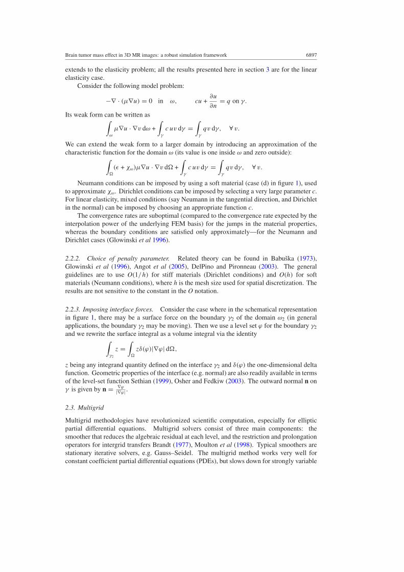
Figure 4. Real brain tumor images, dog case 1 (DC1). From left to right: starting scan, T1MR gadolinium enhanced; target scan, T1 MR gadolinium enhanced; our simulated mass effect,with tumor mask highlighted in white, corresponding to a total pressure P = 4000 Pa, appliedin four equal subsequent pressure increments p = 1000 Pa. Overall deformations are reasonablycaptured.

In figure 5 we show the results of our simulations for the human case. While we appearto have qualitatively captured many of the target scan features (e.g., large displacements ofthe ventricles and corpus callosum), the estimated average relative errors with respect to20 landmarks manually placed by a rater were very large in this case (over 50%). Such acase might be difficult to capture within our simplified framework for the time being. Theenhancing tumor part remains quite small between the two scans, while there is a large masseffect observable at large distances from the enhancing core, which appears to be caused by alarge shadowed area around it, very likely infiltration and edema. In the simulations shown infigure 5, we modeled the edema as a spherical region with a soft material around the tumor,in order to allow for larger deformations. Nevertheless, this introduces additional parametersand accentuates the need for a robust and fully automated optimization procedure in order toimprove agreement with manually placed landmarks.

4. Conclusions and further research

We have presented a general computational framework for soft tissue simulations, targeted onapplications to biomedical imaging and surgical planning. We presently employ it successfullyfor simulating large brain tumor mass effects, with the ultimate purpose of aiding theregistration process for constructing brain tumor atlases. The key components are the use of aregular grid, the choice of appropriate fictitious materials, the fast approximation of forces andboundary conditions within a fully Eulerian frame, and the use of multigrid preconditioners.The main advantages of the method are (1) the ability to deal with complex geometries fast andinexpensive; (2) robustness; (3) algorithmic scalability; (4) minimal memory requirements.The main disadvantage is the theoretically low order of accuracy. For the goal of buildingtumor-bearing brain atlases, the major advantages of the proposed incremental pressure–linearelasticity approach are the following: one can retrieve substantially large deformations fast(order of a couple of minutes) at the end of a relatively small number of pressure steps (e.g.order of ten) at the cost of solving (approximately) one linear algebraic system per step;one has flexibility in simulating and storing intermediate deformation fields, correspondingto various tumor sizes, without restarting the calculations. This translates into a fast, robust

Brain tumor mass effect in 3D MR images: a robust simulation framework 6907

Figure 5. Real brain tumor images, human case (HC). Ewhite = 2100 Pa, Eventricles =500 Pa, νwhite = 0.45, νventricles = 0.1. Overall pressure P = 4000 Pa. From left to right:starting scan, T1 MRI; target scan, T1 MRI; our simulated mass effect.

and flexible simulation tool. We are currently working on enriching our computationalframework to support nonlinear materials and multi-resolution approximations. While theproposed framework can be extended to the nonlinear case (material/geometric nonlinearities),additional inherent complications associated with the actual computational cost must befactored in. Adaptivity is important to further reduce the computational cost, and allowmore accurate approximations in the regions of interest (e.g. close to a tumor boundary).Within our regular grid framework, this can be achieved through the use of tree-based datastructures. We are also working on parallelizing the code to achieve further speedups. Besidesspecific issues related to improving the biomechanical model (e.g. more complex tumor growthmodels, nonlinear material constitutive laws) and speeding up the computational times, anotherdirection we are working on is inverse algorithms for images with brain tumors, where thebiomechanical models, such as the one presented here, are employed as constraints for anobjective function that attempts to maximize the similarities between the actual image and thesimulated one.

Acknowledgment

The first author would like to thank PhD candidates Hari Sundar and Rahul Sampath from theUniversity of Pennsylvania.

References

Alcouffe R E, Brandt A, Dendy Jr J E and Painter J W 1981 The multigrid method for the diffusion equation withstrongly discontinuous coefficients SIAM J. Sci. Stat. Comput. 2 430–54

Angot P et al 2005 A general fictitious domain method with non-conforming structured meshes www.cmi.univ-mrs.fr/ramiere/publis

Babuška Ivo 1973 The finite element method with Lagrangian multipliers Numer. Math. 20 179–92

6908 C Hogea et al

Balay S, Buschelman K, Gropp W D, Kaushik D, McInnes L C and Smith B F 2001 PETSc home pagehttp://www.mcs.anl.gov/petsc

Brandt A 1977 Multi-level adaptive solutions to boundary-value problems Math. Comput. 31 333–90Clatz O, Sermesant M, Bondiau P-Y, Delingette H, Warfield S K, Malandain G and Ayache N 2005 Realistic

simulation of the 3d growth of brain tumors in MR images coupling diffusion with mass effect IEEE Trans.Med. Imaging 24 1334–46

Cotin S, Delingette H and Ayache N 1999 Real-time elastic deformations of soft tissues for surgery simulation IEEETrans. Vis. Comput. Graphics 5 62–73

Davatzikos C 1997 Spatial transformation and registration of brain images using elastically deformable modelsComput. Vis. Image Underst. 66 207–22

Dawant B M, Hartmann S L and Gadamsetty S 1999 Brain atlas deformation in the presence of large space-occupyingtumors MICCAI’99 Proceedings Lecture Notes in Computer Science vol 1679 ed C Taylor and A Colchester(Berlin: Springer) pp 589–96 doi:10.1007/10704282

DelPino S and Pironneau O 2003 A fictitious domain based general PDE solver Numerical Methods for ScientificComputing Variational Problems and Applications (Barcelona)

Ferrant M et al 2001 Registration of 3D intraoperative MR images of the brain using a finite-element biomechanicalmodel IEEE Trans. Med. Imaging 20 1384–97

Glowinski R, Pan T W, Wells R O and Zhou X D 1996 Wavelet and finite element solutions for the Neumann problemusing fictitious domains J. Comput. Phys. 126 40–51

Hagemann A et al 2002 Coupling of fluid and elastic models for biomechanical simulations of brain deformationsusing fem Med. Image Anal. 6 375–88

Hagemann A et al 1999 Biomechanical modeling of the human head for physically based, nonrigid image registrationIEEE Trans. Med. Imaging 18 875–84

Hogea C S 2005 Modeling tumor growth: a computational approach in a continuum framework PhD ThesisBinghamton University

Hogea C S, Murray B T and Sethian J A 2005 Implementation of level set method for continuum mechanics basedtumor growth models Fluid Dyn. Mater. Process. 1 109–30

Hogea C S, Murray B T and Sethian J A 2006 Simulating complex tumor dynamics from avascular to vascular growthusing a general level-set method J. Math. Biol. 53 86–134

Hughes T J R 1987 The Finite Element Method. Linear Static and Dynamic Finite Element Analysis (EnglewoodCliffs, NJ: Prentice-Hall)

Miga M et al Initial in vivo analysis of 3D heterogeneous brain computations for model-updated image-guidedneurosurgery MICCA’98 Proceedings Lecture Notes in Computer Science vol 1496 ed W M Wells, A Colchesterand S Delp (Berlin: Springer) p 743

Mohamed A and Davatzikos C 2005 Finite element modeling of brain tumor mass effect from 3D medical imagesProc. Medical Image Computing and Computer-Assisted Intervention MICCA’05 (Palm Springs) Lecture Notesin Computer Science vol 3749 (Berlin: Springer) pp 400–8

Mohamed A and Davatzikos C 2004 Finite element mesh generation and remeshing from segmented medicalimages Proc. Int. Symp. on Biomedical Imaging: From Nano to Micro (Airlington, Virginia, USA)http://ieeeexplore.ieee.org/iel5/9591/30417/01398564.pdf

Moulton J D, Dendy Jr J E and Hyman J M 1998 The black box multigrid numerical homogenization algorithmJ. Comput. Phys. 142 80–108

Osher S and Fedkiw R 2003 Level Set Methods and Dynamic Implicit Surfaces (Berlin: Springer)Sethian J A 1999 Level Set Methods and Fast Marching Methods (Cambridge: Cambridge University Press)Shah S V et al 1995 The fictitious domain method for patient-specific biomechanical modeling: promise and prospects

2nd Annual Int. Symp. on Medical Robotics and Computer Assisted Surgery, MRCAS ’95 (Pittsburgh, PA:Robotics Institute) p 329

Shewchuk J R 2000 Sweep algorithms for constructing higher-dimensional constrained delaunay triangulations Proc.16th Annual Symposium on Computational Geometry (Kowloon, Hong Kong) (New York: ACM)

Trottenberg U, Oosterlee C W and Schuller A 2000 Multigrid (New York: Academic)Trottenberg U, Oosterlee C W and Schuller A 2001 Multigrid (New York: Academic)Warfield S K et al 2003 Capturing brain deformation Proc. Int. Symp. on Surgery Simulation and Soft Tissue Modeling:

IS4TM 2003 Lecture Notes in Computer Science vol 2673 (Berlin: Springer) p 1001Warfield S K et al 2002 Real-time registration of volumetric brain MRI by biomechanical simulation of deformation

during image-guided neurosurgery Comput. Vis. Sci. 5 3–11Wesseling P 1982 Theoretical and practical aspects of a multigrid method SIAM J. Sci. Stat. Comput. 3 387–407Zacharaki E I, Hogea C S, Biros G and Davatzikos C 2007 A comparative study of biomechanical simulators in

deformable registration of brain tumor images IEEE Trans. Biomed. Eng. at press