Braids and Juggling Patterns Matthew Macauley Michael Orrison

Braids and Juggling Patterns

byMatthew Macauley

Michael Orrison, Advisor

Advisor:

Second Reader:

(Jim Hoste)

May 2003

Department of Mathematics

Abstract

Braids and Juggling Patterns

by Matthew Macauley

May 2003

There are several ways to describe juggling patterns mathematically using com-

binatorics and algebra. In my thesis I use these ideas to build a new system using

braid groups. A new kind of graph arises that helps describe all braids that can be

juggled.

Table of Contents

List of Figures iii

Chapter 1: Introduction 1

Chapter 2: Siteswap Notation 4

Chapter 3: Symmetric Groups 8

3.1 Siteswap Permutations . . . . . . . . . . . . . . . . . . . . . . . . . . . 8

3.2 Interesting Questions . . . . . . . . . . . . . . . . . . . . . . . . . . . . 9

Chapter 4: Stack Notation 10

Chapter 5: Profile Braids 13

5.1 Polya Theory . . . . . . . . . . . . . . . . . . . . . . . . . . . . . . . . . 14


Chapter 6: Braids and Juggling 19

6.1 The Braid Group . . . . . . . . . . . . . . . . . . . . . . . . . . . . . . 19

6.2 Braids of Juggling Patterns . . . . . . . . . . . . . . . . . . . . . . . . . 22

6.3 Counting Jugglable Braids . . . . . . . . . . . . . . . . . . . . . . . . . 24

6.4 Determining Unbraids . . . . . . . . . . . . . . . . . . . . . . . . . . . 27

6.4.1 Setting the crossing numbers to zero. . . . . . . . . . . . . . . 32

6.4.2 The complete system of equations . . . . . . . . . . . . . . . . 37

6.4.3 Simplifying the equations . . . . . . . . . . . . . . . . . . . . . 39

6.5 Adding More Balls . . . . . . . . . . . . . . . . . . . . . . . . . . . . . 42


Appendix A: Appendix 46

A.1 State Graphs . . . . . . . . . . . . . . . . . . . . . . . . . . . . . . . . . 46

A.2 Tables of Sequences . . . . . . . . . . . . . . . . . . . . . . . . . . . . . 48

Bibliography 50

ii

List of Figures

2.1 Profile braid of the pattern 441. . . . . . . . . . . . . . . . . . . . . . . 6

4.1 Relation between siteswap and stack notation. . . . . . . . . . . . . . 11

5.1 Profile braid of the pattern 441. . . . . . . . . . . . . . . . . . . . . . . 13

5.2 A ball crossing the parabola of another ball’s path. . . . . . . . . . . . 14

6.1 A braid on four strings, and an illegal braid. . . . . . . . . . . . . . . 20

6.2 The�th generator of the braid group, �� , and its inverse. . . . . . . . . 20

6.3 The first braid relation: �� if �� . . . . . . . . . . . . . 21

6.4 The second braid relation: �� !�� . . . . . . . . . . . . 21

6.5 An example of the crossing numbers. . . . . . . . . . . . . . . . . . . . 22

6.6 The two types of one-handed juggling throws. . . . . . . . . . . . . . 23

6.7 A non-trivial unbraided juggling pattern: "#��$�%&$�%'"(%'")� . . . . . . . . . . 27

6.8 The Borromean rings, and a braid whose closure is the Borromean

rings. . . . . . . . . . . . . . . . . . . . . . . . . . . . . . . . . . . . . . 28

6.9 How $(% and "*% change the crossing numbers. . . . . . . . . . . . . . . 29

6.10 The stack graph for three-ball juggling patterns. . . . . . . . . . . . . 31

6.11 Realizations of the basis for all unbraids on the stack graph. . . . . . 34

6.12 Different realizations of the basis element +,� . . . . . . . . . . . . . . . 36

6.13 Labeling the edges of the stack graph. . . . . . . . . . . . . . . . . . . 37

6.14 A length-four unbraid. . . . . . . . . . . . . . . . . . . . . . . . . . . . 41

6.15 The condensed three-ball stack graph. . . . . . . . . . . . . . . . . . . 42

iii

6.16 Two ways to view the four-ball condensed graph. . . . . . . . . . . . 43

6.17 The stack graph of four-ball juggling patterns. . . . . . . . . . . . . . 44

A.1 The state graph �� . . . . . . . . . . . . . . . . . . . . . . . . . . . . 47

iv

Acknowledgments

I would like to thank my advisors Michael Orrison and Jim Hoste for helping

me with my research. I would also like to thank fellow jugglers and mathemati-

cians Ron Graham and Will Murray for letting me bounce ideas off of them and

giving me feedback.

v

Chapter 1

Introduction

Mathematics and juggling have both been around for thousands of years. The

oldest known record of juggling was recovered from a burial site in Egypt that is

nearly four thousand years old. Evidence of juggling has been uncovered in the

histories of many different civilizations, including ancient China, Europe, Asia,

and the Middle East. Though both have elaborate histories, mathematics and jug-

gling have only become intertwined within the last few decades. The big break-

through came in 1985 when three different sources independently invented a math-

ematical notation for juggling patterns. These groups were Caltech students Bengt

Magnusson and Bruce Tiemann, the trio of Mike Day, Colin Wright and Adam

Chalcraft from Cambridge, and Paul Klimak at the University of California, Santa

Cruz. The notation, called siteswap notation, describes a juggling pattern by a

sequence of digits that denote the height of each throw.

There are several different mathematical aspects of juggling that have been ex-

amined. One natural topic is the physics of juggling. Magnusson and Tiemann

published a paper [2] on this subject in 1989. A decade later, Jack Kalvin, a profes-

sional juggler who holds a mechanical engineering degree from Carnegie Mellon

University, wrote two papers [6, 7] in the late 1990s about the physics of juggling.

One of his results is determining how many balls a human being can physically

juggle. He uses the first four time derivatives of the motion of the juggler’s throw-

ing hand to conclude that it should be physically possible for a human being to

2

juggle up to fifteen balls. However, the current record stands at ten, where the

juggler must make �� catches of � balls for it to qualify as a “juggle.” Several in-

dividuals have been able to “flash” twelve balls, which means each ball is thrown

and caught once. Recently, Albert Lucas successfully flashed fourteen rings. No-

body else has flashed more than twelve.

There are connections between siteswap notation and physics. However, siteswap

notation in itself poses many interesting algebraic and combinatorial questions.

One of the big papers in this area was co-authored by Joe Buhler, David Eisenbud,

Ron Graham and Colin Wright in 1994 [3]. They used some innovative techniques

to count the number of siteswap patterns of a fixed length given a certain number

of balls. They wrote a second paper that generalized the mathematics they had in-

vented in their first paper to any arbitrary partially ordered set. Another important

paper was written by Richard Ehrenborg and Margret Readdy in 1996. Siteswap

notation can be generalized to describe patterns, called multiplex patterns, where a

hand can throw more than one ball at a time. Ehrenborg and Readdy provided con-

nections between multiplexed patterns and Stirling numbers of the second kind,

and the affine Weyl group�� .

Eighteen months prior to writing this thesis, I had the idea of studying siteswap

patterns by looking at the braid formed by attaching strings to the ends of the balls.

A more natural way to make a braid when juggling is to walk forward and look

at the braid formed by the paths of the balls traced out in space. I searched far

and wide to see if this had been done before and found nothing to suggest that it

had. A year later when I began this thesis, I searched again. This time, I found

a website linked from the juggling club at Brown University [8]. For a project in

an undergraduate topology class, two students had looked at braid groups and

realized that juggling patterns can be represented as braids in this manner. They

gave a few examples of the braids of some simple siteswap patterns and discussed

some general concepts. A few months later, Burkard Polster published a book

3

about the mathematics of juggling that was intended to be a collection of just about

everything that has been done so far with mathematics and juggling [9]. He talks

about braids and juggling for about five pages, mostly summarizing what had

been said in [8], and proving the theorem that with enough hands, any braid can

be juggled. The result is intuitive, and follows from the fact that any braid can be

generated by a series of crossings of adjacent strings.

In this paper I give some background of the mathematics of juggling needed

to study the braids of juggling patterns, which is the focus of Chapter 6. At the

end of each chapter, I pose some questions that arose when working on this paper.

They are not necessarily extremely difficult, but just ideas that I had but never got

around to when working on this paper. Some of them are natural generalizations

that may or may not have promise. However, I am confident that there is lots of

room for future research about the mathematics of juggling.

Chapter 2

Siteswap Notation

In order to examine the mathematics of juggling we must set some rules for

what constitutes a valid juggling pattern with � balls. First we need a notion of

equal time intervals, or beats. Throws may only be made on a beat, and at most

one ball is thrown or caught each beat. In practice, once a ball lands, it remains in

the juggler’s hand for at least a beat before it is thrown again. However, once a ball

is thrown we will only concern ourselves with the number of beats before that ball

is thrown again. Any juggling pattern can be described by the function �� where the ball thrown at time � is thrown next at time � �� . If no ball is thrown at

time �� , then � �� . Because balls are not thrown back in time, to each pattern

we assign a non-negative height function

� ��

defined by� ��

For every beat � , � �� is the number of beats from when the ball thrown at time

� will be thrown again. Notice that a height of 0 means that there was no throw

on that beat. In this paper we shall only consider patterns with periodic height

functions, which means that for some �� , � �� . For any positive �that satisfies this condition, we define the function

� �� !��

5

by� �� . Every � -periodic pattern can be described as a length- � string of

non-negative digits, namely

� � � � � � � ��

This is called siteswap notation, and a juggling pattern in this form is called a

siteswap pattern. In practice, most siteswap patterns that people juggle do not have

throws higher than a seven. Even the most advanced jugglers rarely will juggle a

pattern with a throw higher than a nine. There are a few exceptions, and for these

patterns, letters are used for higher digits, like A=10, B=11, C=12, and so on.

Several properties are immediate consequences of the construction of siteswap

notation. Since two balls cannot land on the same beat, for any positive integer�,� ��

. Also, with � balls, the average height must be � , and so the

average of the digits of a siteswap pattern is the number of balls in that pattern. To

give a few examples, some common three-ball patterns are 3, 51, 423, 441, 504, 531,

and 51414.

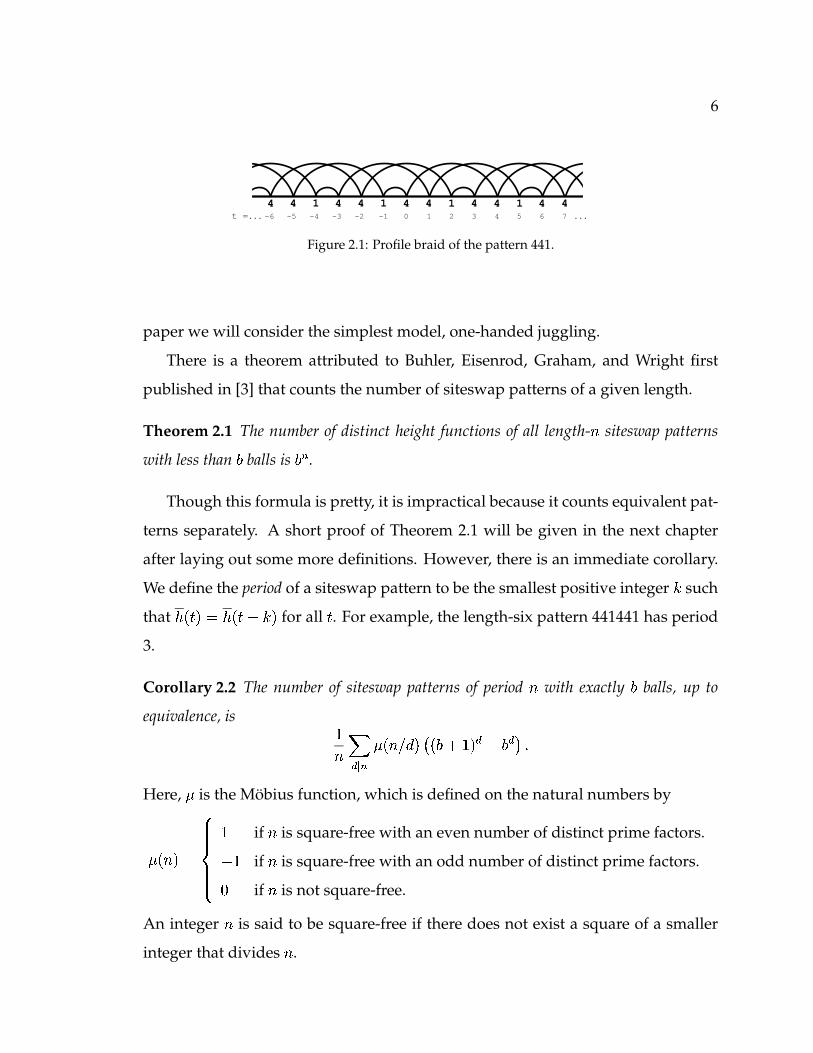
One way to think of a siteswap pattern is to use a profile braid. For a siteswap

pattern with height function�

, an arc is drawn on the real line from � to � � � �� for

each integer � . The profile braid depicts the paths of the balls of a pattern as seen

from the side as the jugglers walks forward. Figure 2.1 is the profile braid of the

pattern 441. Profile braids will be discussed in more detail in Chapter 5. Notice

that the patterns 441, 414, and 144 all yield the same profile braid, only shifted.

We will call two siteswap patterns with height functions� � and

� % equivalent if for

some integer � , � � �� )� � % �� for all � . Hence, 441, 414, and 144 are all equivalent.

Siteswap notation does not describe how many hands are used to juggle the

pattern or the locations of the hands. The standard juggling method uses two

hands that alternate throwing the balls. Balls are caught from the outside of the

pattern and thrown from the inside. Observe that using this convention, throws

with even heights don’t switch hands while throws with odd heights do. In this

6

4 4 4 4 4 4 41 1 1 4 1 4 44 53210 6 7-1-2-3-4-5-6...t = ...

Figure 2.1: Profile braid of the pattern 441.

paper we will consider the simplest model, one-handed juggling.

There is a theorem attributed to Buhler, Eisenrod, Graham, and Wright first

published in [3] that counts the number of siteswap patterns of a given length.

Theorem 2.1 The number of distinct height functions of all length- � siteswap patterns

with less than � balls is �� .

Though this formula is pretty, it is impractical because it counts equivalent pat-

terns separately. A short proof of Theorem 2.1 will be given in the next chapter

after laying out some more definitions. However, there is an immediate corollary.

We define the period of a siteswap pattern to be the smallest positive integer � such

that� �� for all � . For example, the length-six pattern 441441 has period

3.

Corollary 2.2 The number of siteswap patterns of period � with exactly � balls, up to

equivalence, is ��

��

��

Here, � is the Mobius function, which is defined on the natural numbers by

� � � �)��

if � is square-free with an even number of distinct prime factors.� �

if � is square-free with an odd number of distinct prime factors.

� if � is not square-free.

An integer � is said to be square-free if there does not exist a square of a smaller

integer that divides � .

7

Proof: By Theorem 2.1, there are � � � � � � � � � different height functions that de-

scribe a � -ball juggling pattern. However, this over-counts the number of siteswap

patterns because different height functions can correspond to equivalent siteswap

patterns. Let � � � � � � be the number of siteswap patterns of period � with exactly �balls. For every divisor � of � , there are � �� equivalent patterns of period � , related

by shifting the digits. We can count the length- � height functions by summing over

all height functions of length � for each �� . Thus

� ��

We can solve for � � � � � � using a combinatorial technique called a Mobius inversion

to get

� � � � � � ��

��

��

Mobius inversion is described in [13]. �

Chapter 3

Symmetric Groups

3.1 Siteswap Permutations

Let S � be the group of all permutations of the set � �� .Every periodic height function

�of a length- � pattern naturally corresponds to a

permutation that sends each integer�� , the domain of

�, to

� � � �� modulo � .

One way to think of this is a beat �� mod � � is sent to the beat reduced modulo

� where the ball thrown on � will be thrown next. Notice that if a no ball is thrown

on beat�, then the permutation sends

�to itself. This is a permutation because no

more than one ball is thrown each beat and at most one ball lands each beat. We

can define this map

� � � length � siteswap patterns � �� S �because each siteswap pattern corresponds to a unique

�function. However, � is

not injective. Several siteswap patterns can give rise to the same permutation. As

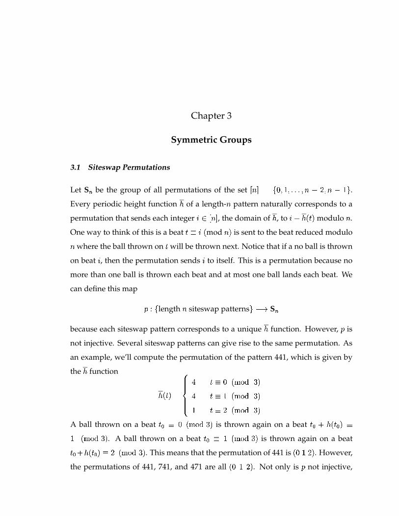
an example, we’ll compute the permutation of the pattern 441, which is given by

the�

function

� �� )�

� � ��

A ball thrown on a beat � �� is thrown again on a beat � � � �� . A ball thrown on a beat � �� is thrown again on a beat

�� . This means that the permutation of 441 is � � � � � . However,

the permutations of 441, 741, and 471 are all � � � � � . Not only is � not injective,

9

but equivalent juggling patterns may even have different permutations. As an ex-

ample, the pattern 423 has permutation � � � � � � � but the equivalent pattern 342 has

permutation � � � � � � � . In order to have equivalent patterns correspond to the same

permutation, we need to put an equivalence relation on the set of permutations.

We shall call two permutations in � � equivalent if they describe equivalent

siteswap patterns. For any siteswap pattern with permutation � , the equivalent

siteswap pattern obtained by beginning with the�th digit corresponds to the per-

mutation resulting in incrementing each digit in the cycle notation of � by�

modulo

� . For example, � � � � � � � � � � � � � � � � �� and � �� .Later we will see that if two profile braids as described in Chapter 5 are in the

same same orbit of� � acting on the set of period- � profile braids, they have the

equivalent permutations. The converse is false.

3.2 Interesting Questions

1. How many distinct elements of � � are there up to equivalence?

2. If a pattern has permutation � , then what can we say about patterns that have

permutation �

� � ?

3. Are there any similarities between patterns whose permutations are conju-

gate?

Chapter 4

Stack Notation

At any time during a juggling pattern, we can make an ordered list of the balls

in the air based on the order that they will land. If we assign each ball a unique

color, then we can draw a vertical stack of colors in order of the landing times of

the balls, with the lowest ball landing first. Each time we throw a ball, that ball gets

inserted somewhere into the stack of the other � � � balls. There are � slots to insert

the new ball, and if we label them from bottom-to-top� �!� � � � � � � , we can create a

length- � sequence for every siteswap pattern. If no ball is thrown at a beat, then

the digit at the beat is 0 and the stack remains unchanged. We call one of these

sequences the stack sequence of a juggling pattern.

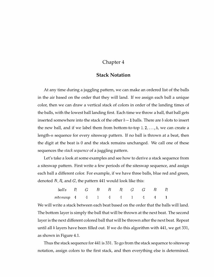
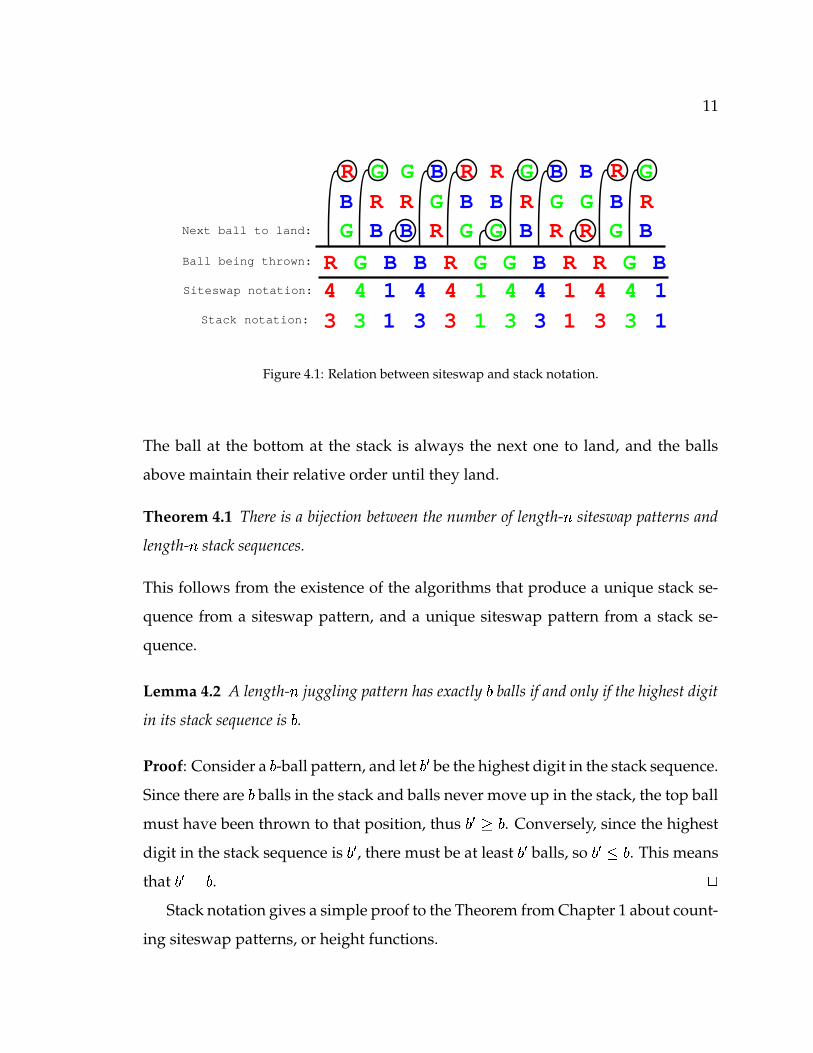
Let’s take a look at some examples and see how to derive a stack sequence from

a siteswap pattern. First write a few periods of the siteswap sequence, and assign

each ball a different color. For example, if we have three balls, blue red and green,

denoted � �� , and � , the pattern 441 would look like this:

��

� ��

We will write a stack between each beat based on the order that the balls will land.

The bottom layer is simply the ball that will be thrown at the next beat. The second

layer is the next different colored ball that will be thrown after the next beat. Repeat

until all � layers have been filled out. If we do this algorithm with 441, we get 331,

as shown in Figure 4.1.

Thus the stack sequence for 441 is 331. To go from the stack sequence to siteswap

notation, assign colors to the first stack, and then everything else is determined.

11

B

R G B B R G G B R4 4 1 4 4 1 4 4 1

3 3 1 3 3 1 3 3 1

R

BG B

R

G

BR

G

RG

B

GB

R

GB

R

BR

G

R

B

G

4 4 1

3 3 1

R G B

RG

GB

R

BR

G

Siteswap notation:

Stack notation:

Ball being thrown:

Next ball to land:

Figure 4.1: Relation between siteswap and stack notation.

The ball at the bottom at the stack is always the next one to land, and the balls

above maintain their relative order until they land.

Theorem 4.1 There is a bijection between the number of length- � siteswap patterns and

length- � stack sequences.

This follows from the existence of the algorithms that produce a unique stack se-

quence from a siteswap pattern, and a unique siteswap pattern from a stack se-

quence.

Lemma 4.2 A length- � juggling pattern has exactly � balls if and only if the highest digit

in its stack sequence is � .

Proof: Consider a � -ball pattern, and let �� be the highest digit in the stack sequence.

Since there are � balls in the stack and balls never move up in the stack, the top ball

must have been thrown to that position, thus � � � � . Conversely, since the highest

digit in the stack sequence is � � , there must be at least � � balls, so � � � � . This means

that �� . �

Stack notation gives a simple proof to the Theorem from Chapter 1 about count-

ing siteswap patterns, or height functions.

12

Corollary 4.3 There are � � � � � � siteswap patterns of length- � using at most � balls, and

� � zeros are disallowed.

Proof: The number of length- � stack sequences with at most � balls is the number

of sequences using the digits� � � � � � � � � � � , which is � � � � � � . If zeros are not allowed,

then it is just � � . Because there is a bijection between stack sequences and siteswap

patterns (or height functions), this is also the number of siteswap patterns. �

Chapter 5

Profile Braids

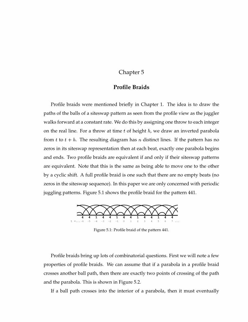
Profile braids were mentioned briefly in Chapter 1. The idea is to draw the

paths of the balls of a siteswap pattern as seen from the profile view as the juggler

walks forward at a constant rate. We do this by assigning one throw to each integer

on the real line. For a throw at time � of height�

, we draw an inverted parabola

from � to � � � . The resulting diagram has � distinct lines. If the pattern has no

zeros in its siteswap representation then at each beat, exactly one parabola begins

and ends. Two profile braids are equivalent if and only if their siteswap patterns

are equivalent. Note that this is the same as being able to move one to the other

by a cyclic shift. A full profile braid is one such that there are no empty beats (no

zeros in the siteswap sequence). In this paper we are only concerned with periodic

juggling patterns. Figure 5.1 shows the profile braid for the pattern 441.

4 4 4 4 4 4 41 1 1 4 1 4 44 53210 6 7-1-2-3-4-5-6...t = ...

Figure 5.1: Profile braid of the pattern 441.

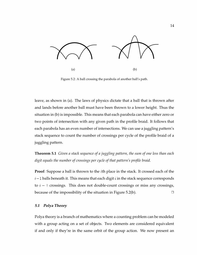
Profile braids bring up lots of combinatorial questions. First we will note a few

properties of profile braids. We can assume that if a parabola in a profile braid

crosses another ball path, then there are exactly two points of crossing of the path

and the parabola. This is shown in Figure 5.2.

If a ball path crosses into the interior of a parabola, then it must eventually

14

(a) (b)

Figure 5.2: A ball crossing the parabola of another ball’s path.

leave, as shown in (a). The laws of physics dictate that a ball that is thrown after

and lands before another ball must have been thrown to a lower height. Thus the

situation in (b) is impossible. This means that each parabola can have either zero or

two points of intersection with any given path in the profile braid. It follows that

each parabola has an even number of intersections. We can use a juggling pattern’s

stack sequence to count the number of crossings per cycle of the profile braid of a

juggling pattern.

Theorem 5.1 Given a stack sequence of a juggling pattern, the sum of one less than each

digit equals the number of crossings per cycle of that pattern’s profile braid.

Proof: Suppose a ball is thrown to the�th place in the stack. It crossed each of the

� � �balls beneath it. This means that each digit

�in the stack sequence corresponds

to� � �

crossings. This does not double-count crossings or miss any crossings,

because of the impossibility of the situation in Figure 5.2(b). �

5.1 Polya Theory

Polya theory is a branch of mathematics where a counting problem can be modeled

with a group acting on a set of objects. Two elements are considered equivalent

if and only if they’re in the same orbit of the group action. We now present an

15

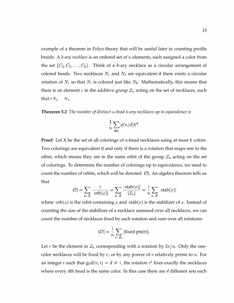
example of a theorem in Polya theory that will be useful later in counting profile

braids. A k-ary necklace is an ordered set of � elements, each assigned a color from

the set�� % � � � � � � � � . Think of a � -ary necklace as a circular arrangement of

colored beads. Two necklaces � � and � % are equivalent if there exists a circular

rotation of � � so that � � is colored just like � % . Mathematically, this means that

there is an element � in the additive group� � acting on the set of necklaces, such

that �� )�� % .

Theorem 5.2 The number of distinct � -bead � -ary necklaces up to equivalence is��

��

Proof: Let X be the set of all colorings of � -bead necklaces using at most � colors.

Two colorings are equivalent if and only if there is a rotation that maps one to the

other, which means they are in the same orbit of the group� � acting on the set

of colorings. To determine the number of colorings up to equivalence, we need to

count the number of orbits, which will be denoted �� . An algebra theorem tells us

that

��

� orb ��

��

stab ��

��

stab ��

where orb �� is the orbit containing and stab �� is the stabilizer of . Instead of

counting the size of the stabilizer of a necklace summed over all necklaces, we can

count the number of necklaces fixed by each rotation and sum over all rotations:

��

��

fixed pts(r) �

Let � be the element in� � corresponding with a rotation by � � � . Only the one-

color necklaces will be fixed by � , or by any power of � relatively prime to � . For

an integer�

such that gcd � � � � � � � �� , the rotation � � fixes exactly the necklaces

where every � th bead is the same color. In this case there are � different sets each

16

containing � �� beads, and so we have �

�possible colorings that are fixed by � � .

There are� � � �� rotations � � such that gcd � � � � � � � . Summing over all rotations,

we get ��

�

which proves the theorem. �

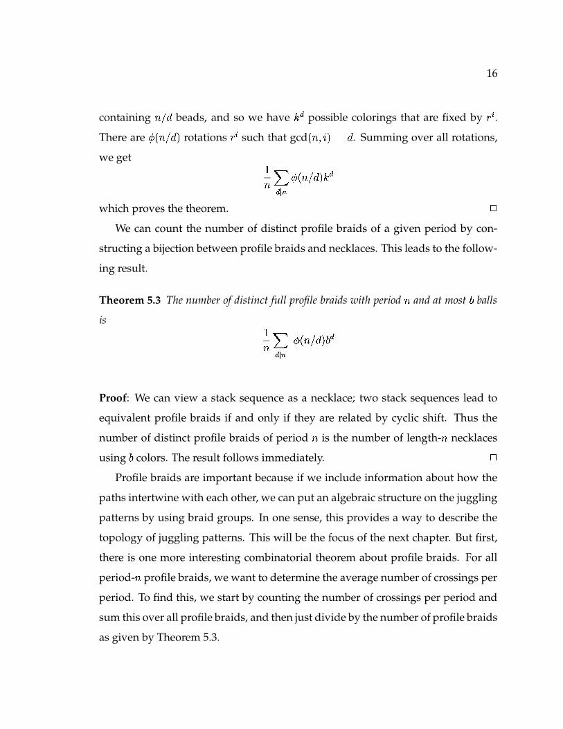
We can count the number of distinct profile braids of a given period by con-

structing a bijection between profile braids and necklaces. This leads to the follow-

ing result.

Theorem 5.3 The number of distinct full profile braids with period � and at most � balls

is ��

� � � ��

Proof: We can view a stack sequence as a necklace; two stack sequences lead to

equivalent profile braids if and only if they are related by cyclic shift. Thus the

number of distinct profile braids of period � is the number of length- � necklaces

using � colors. The result follows immediately. �

Profile braids are important because if we include information about how the

paths intertwine with each other, we can put an algebraic structure on the juggling

patterns by using braid groups. In one sense, this provides a way to describe the

topology of juggling patterns. This will be the focus of the next chapter. But first,

there is one more interesting combinatorial theorem about profile braids. For all

period- � profile braids, we want to determine the average number of crossings per

period. To find this, we start by counting the number of crossings per period and

sum this over all profile braids, and then just divide by the number of profile braids

as given by Theorem 5.3.

17

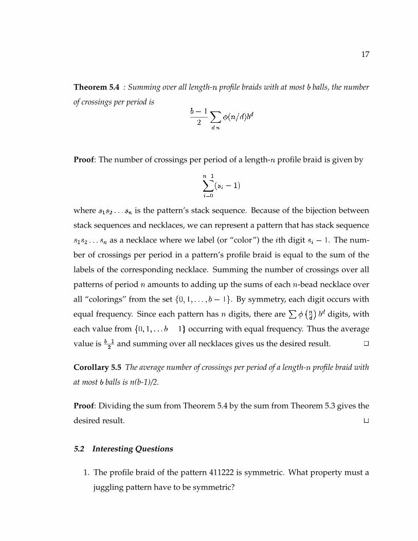
Theorem 5.4 : Summing over all length- � profile braids with at most � balls, the number

of crossings per period is� ��

� ��

�

Proof: The number of crossings per period of a length- � profile braid is given by

� � ��

� � �

where � % � � �� is the pattern’s stack sequence. Because of the bijection between

stack sequences and necklaces, we can represent a pattern that has stack sequence

� % � � �� as a necklace where we label (or “color”) the�th digit � � � . The num-

ber of crossings per period in a pattern’s profile braid is equal to the sum of the

labels of the corresponding necklace. Summing the number of crossings over all

patterns of period � amounts to adding up the sums of each � -bead necklace over

all “colorings” from the set� � � � � � � � � � � � � . By symmetry, each digit occurs with

equal frequency. Since each pattern has � digits, there are� � � �

��

�digits, with

each value from� � � � � � � � � � � � occurring with equal frequency. Thus the average

value is �� % and summing over all necklaces gives us the desired result. �

Corollary 5.5 The average number of crossings per period of a length- � profile braid with

at most � balls is n(b-1)/2.

Proof: Dividing the sum from Theorem 5.4 by the sum from Theorem 5.3 gives the

desired result. �


1. The profile braid of the pattern 411222 is symmetric. What property must a

juggling pattern have to be symmetric?

18

2. The profile braids of 411231 and 411321 are mirror images of each other. Find

necessary and sufficient conditions for two juggling patterns to have profile

braids that are mirror images of each other.

3. We can model bounced throws by allowing both regular and inverted parabo-

las in the profile braid. Prove similar results for this generalization.

Chapter 6

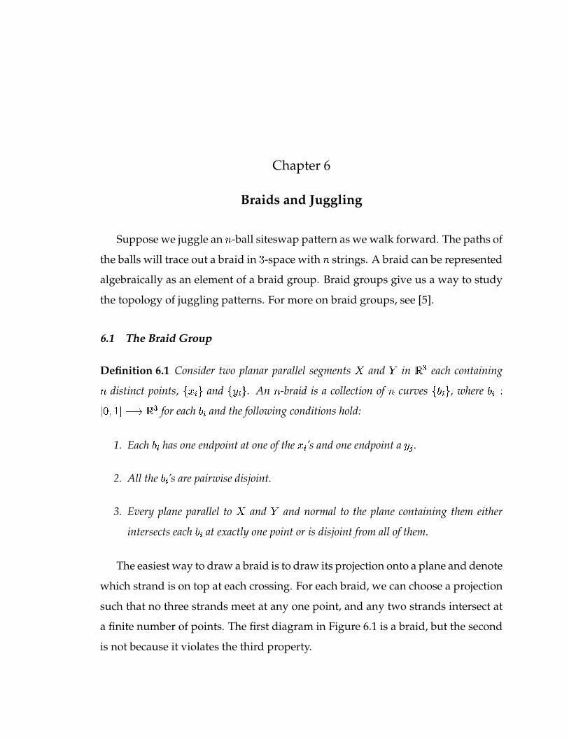
Braids and Juggling

Suppose we juggle an � -ball siteswap pattern as we walk forward. The paths of

the balls will trace out a braid in � -space with � strings. A braid can be represented

algebraically as an element of a braid group. Braid groups give us a way to study

the topology of juggling patterns. For more on braid groups, see [5].

6.1 The Braid Group

Definition 6.1 Consider two planar parallel segments + and � in �� each containing

� distinct points,� �� and

�� . An � -braid is a collection of � curves� �&� � , where ��

� � � � � �� for each �� and the following conditions hold:

1. Each �� has one endpoint at one of the � ’s and one endpoint a� � .

2. All the �� ’s are pairwise disjoint.

3. Every plane parallel to + and � and normal to the plane containing them either

intersects each �!� at exactly one point or is disjoint from all of them.

The easiest way to draw a braid is to draw its projection onto a plane and denote

which strand is on top at each crossing. For each braid, we can choose a projection

such that no three strands meet at any one point, and any two strands intersect at

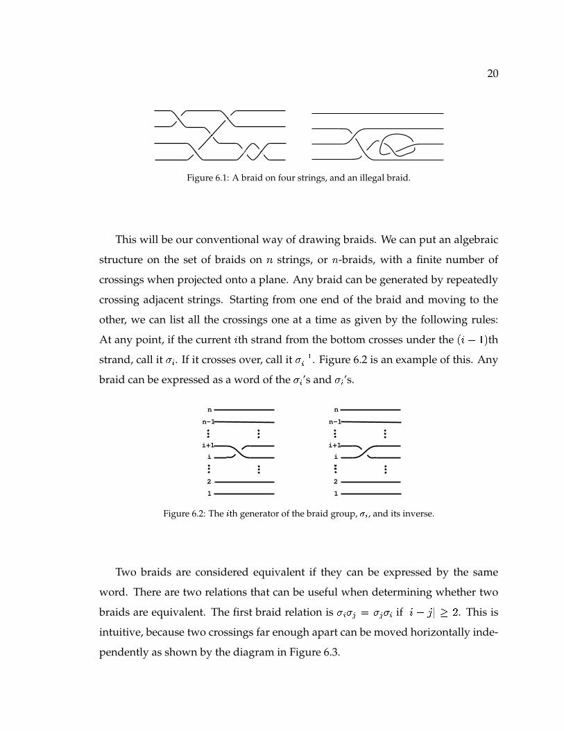
a finite number of points. The first diagram in Figure 6.1 is a braid, but the second

is not because it violates the third property.

20

Figure 6.1: A braid on four strings, and an illegal braid.

This will be our conventional way of drawing braids. We can put an algebraic

structure on the set of braids on � strings, or � -braids, with a finite number of

crossings when projected onto a plane. Any braid can be generated by repeatedly

crossing adjacent strings. Starting from one end of the braid and moving to the

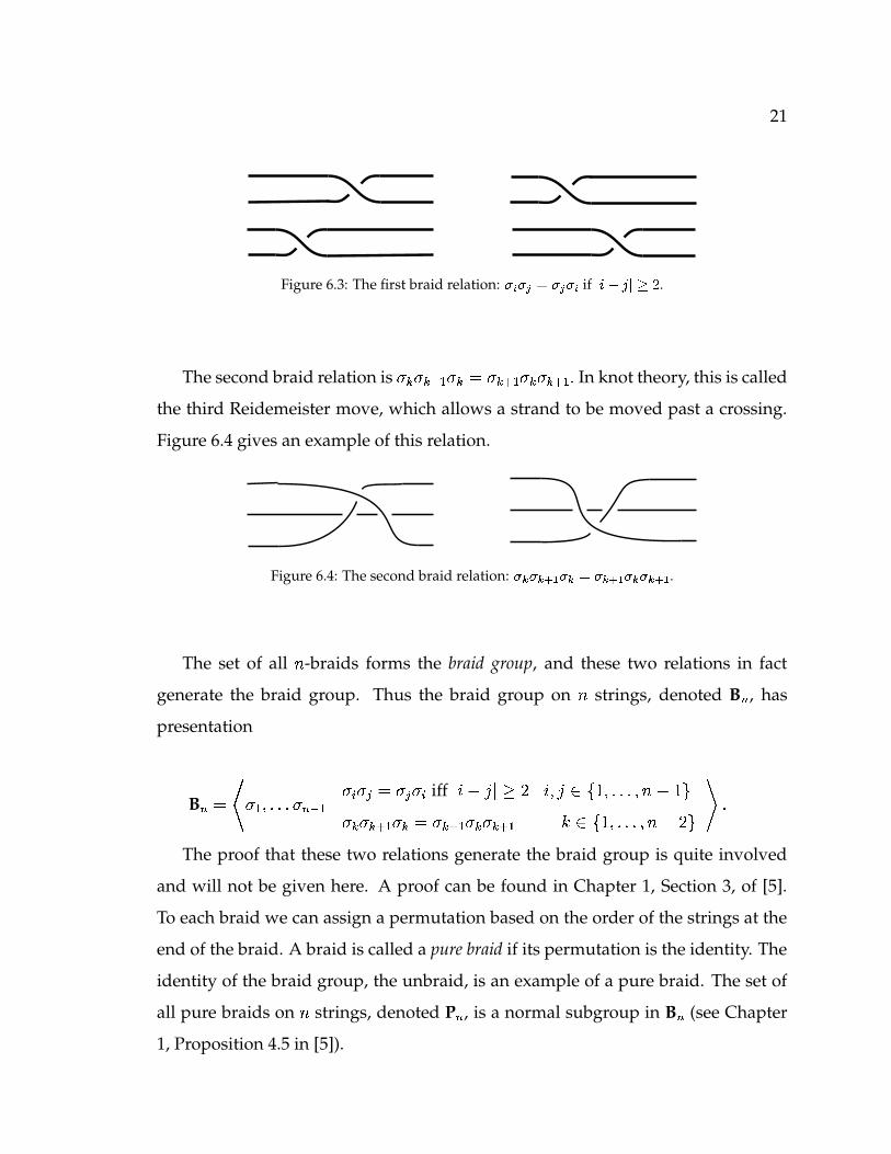
other, we can list all the crossings one at a time as given by the following rules:

At any point, if the current�th strand from the bottom crosses under the � � � � � th

strand, call it �� . If it crosses over, call it �� . Figure 6.2 is an example of this. Any

braid can be expressed as a word of the �� ’s and �� ’s.

1

2

i

i+1

n

n-1

1

2

i

i+1

n

n-1

Figure 6.2: The � th generator of the braid group, �� , and its inverse.

Two braids are considered equivalent if they can be expressed by the same

word. There are two relations that can be useful when determining whether two

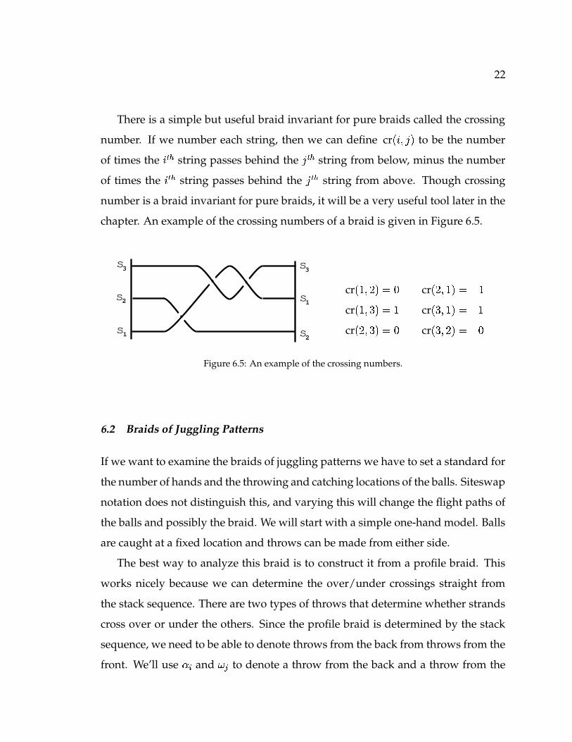
braids are equivalent. The first braid relation is � �� if �)� � (� � . This is

intuitive, because two crossings far enough apart can be moved horizontally inde-

pendently as shown by the diagram in Figure 6.3.

21

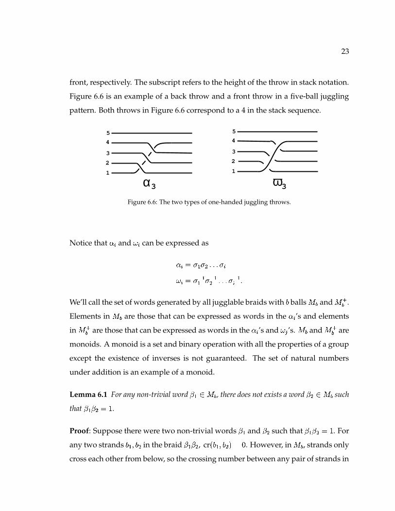
Figure 6.3: The first braid relation: � � � �� if � �� .The second braid relation is �� !�� !�� In knot theory, this is called

the third Reidemeister move, which allows a strand to be moved past a crossing.

Figure 6.4 gives an example of this relation.

Figure 6.4: The second braid relation: �� .The set of all � -braids forms the braid group, and these two relations in fact

generate the braid group. Thus the braid group on � strings, denoted B � , has

presentation

B � �� !� � � ��

�� iff ��

The proof that these two relations generate the braid group is quite involved

and will not be given here. A proof can be found in Chapter 1, Section 3, of [5].

To each braid we can assign a permutation based on the order of the strings at the

end of the braid. A braid is called a pure braid if its permutation is the identity. The

identity of the braid group, the unbraid, is an example of a pure braid. The set of

all pure braids on � strings, denoted P � , is a normal subgroup in B � (see Chapter

1, Proposition 4.5 in [5]).

22

There is a simple but useful braid invariant for pure braids called the crossing

number. If we number each string, then we can define cr � � � � � to be the number

of times the��

string passes behind the��

string from below, minus the number

of times the��

string passes behind the��

string from above. Though crossing

number is a braid invariant for pure braids, it will be a very useful tool later in the

chapter. An example of the crossing numbers of a braid is given in Figure 6.5.

s

s

s

3

2

1

s3

s2

s1cr � � �!� � � � cr � � � � � � � �cr � � � � � � � cr � � � � � � �

cr � � � � � � � cr � � �!� � � �

Figure 6.5: An example of the crossing numbers.

6.2 Braids of Juggling Patterns

If we want to examine the braids of juggling patterns we have to set a standard for

the number of hands and the throwing and catching locations of the balls. Siteswap

notation does not distinguish this, and varying this will change the flight paths of

the balls and possibly the braid. We will start with a simple one-hand model. Balls

are caught at a fixed location and throws can be made from either side.

The best way to analyze this braid is to construct it from a profile braid. This

works nicely because we can determine the over/under crossings straight from

the stack sequence. There are two types of throws that determine whether strands

cross over or under the others. Since the profile braid is determined by the stack

sequence, we need to be able to denote throws from the back from throws from the

front. We’ll use $ � and "�� to denote a throw from the back and a throw from the

23

front, respectively. The subscript refers to the height of the throw in stack notation.

Figure 6.6 is an example of a back throw and a front throw in a five-ball juggling

pattern. Both throws in Figure 6.6 correspond to a 4 in the stack sequence.

1

2

4

5

3

α3

1

2

4

5

3

ω3

Figure 6.6: The two types of one-handed juggling throws.

Notice that $ � and " � can be expressed as

$ � �� % � � �!��" � ��

� �� % � � ��

� ��

We’ll call the set of words generated by all jugglable braids with � balls � � and � ��

.

Elements in � � are those that can be expressed as words in the $�� ’s and elements

in � ��

are those that can be expressed as words in the $ � ’s and " � ’s. � � and � ��

are

monoids. A monoid is a set and binary operation with all the properties of a group

except the existence of inverses is not guaranteed. The set of natural numbers

under addition is an example of a monoid.

Lemma 6.1 For any non-trivial word� � � � � , there does not exists a word

� % � � � such

that� � � % � � .

Proof: Suppose there were two non-trivial words� � and

� % such that� � � % � � . For

any two strands � � � � % in the braid� � � % , cr � � � � � % � � � . However, in � � , strands only

cross each other from below, so the crossing number between any pair of strands in

24

a non-trivial word in � � is positive. Thus cr � � � � � % � � � , so� � � % is not the unbraid.

�

6.3 Counting Jugglable Braids

Counting braids is a delicate issue. Consider the patterns 42 and 24, which give

rise to the braids $ �'$�% and $(%!$ � , respectively. One typically juggles for more than

just one cycle, in which case both of these patterns would be � � �� ,and would look exactly the same to an observer. We shall consider two braids

� �and

� % the same if� � and

� % can be expressed as

� � �� % ��'�� !��

such that for some integer � ,

� % �� &�� !��

This simply means that the word expressing� � can be cyclically permuted into the

word expressing� % .

The next goal is to count the number of different braids that can arise from a

length- � siteswap pattern with � balls. Recall that a � -ball pattern must have at least

one � in its stack-sequence, and that 0’s and 1’s in the stack sequence have no effect

on the braid. Because of this, the braids of the stack sequences 312, 321, and 32 all

lead to the braid $(%&$ � . Since any pattern of length less than � can be lengthened by

adding 0’s or 1’s without changing the braid, we only need to count the number of

stack sequences without 0’s or 1’s, containing at least one � , with period at most � .

First of all, we’ll consider just one type of throws, namely the $ � ’s.

Theorem 6.2 The number of distinct braids in � � arising from length- � juggling patterns

25

is at most �� )� �

��

��

� ��

Proof: Let � � � � � � � be the number of stack sequences with period � with � balls

that contain no 0’s or 1’s. Because there are � � � � � � stack sequences with at most

� balls and � � � � � � sequences with at most � � � balls, there are � � � � � � � � � � � � �length- � stack sequences with exactly � balls. Each length- � sequence with period� , where � is a divisor of � , is equivalent to � different stack sequences (juggling

patterns). Therefore, we can write

� � � � � � � � � � � � � � � ��

By Mobius inversion, we can solve for � � � � � � � and get

� � � � � � � ��

��

��

For any stack sequence of length less than � , we can insert 0’s and 1’s anywhere

in the sequence and not change the braid. Therefore, the number of distinct braids

taken over all length- � juggling patterns is at most��

��

��

� �

which proves the theorem. �

We stress “at most” in Theorem 6.2 because two braids arising from different

juggling patterns may be the same braid. For example, consider the siteswap pat-

terns 33 and 522. The stack sequence of these patterns are 33 and 232, respectively,

which means that their braids are $*%!$�% and $ �'$�%!$ � . Using the second braid relation

we can conclude

$�%&$�% ��'� %&��'� %$ �'$�%!$ �)�� %!� �)�� %&��%!� �

26

which means that the patterns 33 and 522 have the equivalent braids when juggled

in � � . A juggler might appreciate this fact because when juggled with two hands,

33 (or 3) is called the “cascade,” and pattern 522 is called the “slow cascade.” Be-

cause in practice, most people treat 2’s as just holds, 522 is just a higher and slower

cascade, and it makes sense that they have the same braid. It is surprising that

these two patterns also have the same braid when juggled with one hand. How-

ever, it is not true in general that if two siteswap patterns have the same braid with

two hands, then they have the same braid with one hand. In fact, it seems that in

most cases they do not have the same braid.

A simple corollary of Theorem 6.2 is an upper bound on the number of braids

in � ��

arising from length- � juggling patterns.

Corollary 6.3 The number of braids in � ��

arising from length- � juggling patterns is at

most �� )� �

��

��

��

Proof: If both front and back throws are allowed as in � ��

, then for each digit�

in

the stack sequence, there are two possible throws: $�� and " � � � . This means that

each length- � pattern in � � gives rise to at most � � possible braids in � ��

. Thus,

the number of braids corresponding with length- � patterns is at most�� )� �

��

��

��

�

Appendix B contains some tables with the values of the upper bounds of the

number of braids arising from length- � patterns in the monoids of � -ball juggling

braids, � � and � ��

, for small values of � and � .

27

6.4 Determining Unbraids

A non-trivial unbraid is a word of at least one generator that is equivalent to the

unbraid. A natural question that arises about the monoids � � and � ��

is whether

or not they contain any non-trivial unbraids. It is not difficult to show that � �does not contain any non-trivial unbraids. Every element except the identity in � �has at least one pair of strands � � � � � such that cr � � � � � � � . And it is impossible

to get any pair of strands to have a negative crossing number. In order to get a

non-trivial unbraid, the sum of the crossing numbers of every pair of stands must

be zero. This is impossible using just words in the $ � ’s.

However, this argument does not work for � ��

. Right away we see that $ � ")�is an unbraid, and we can concatenate this to itself to get an infinite family of

unbraids. In fact, these are not the only unbraids in � ��

. One such example, the

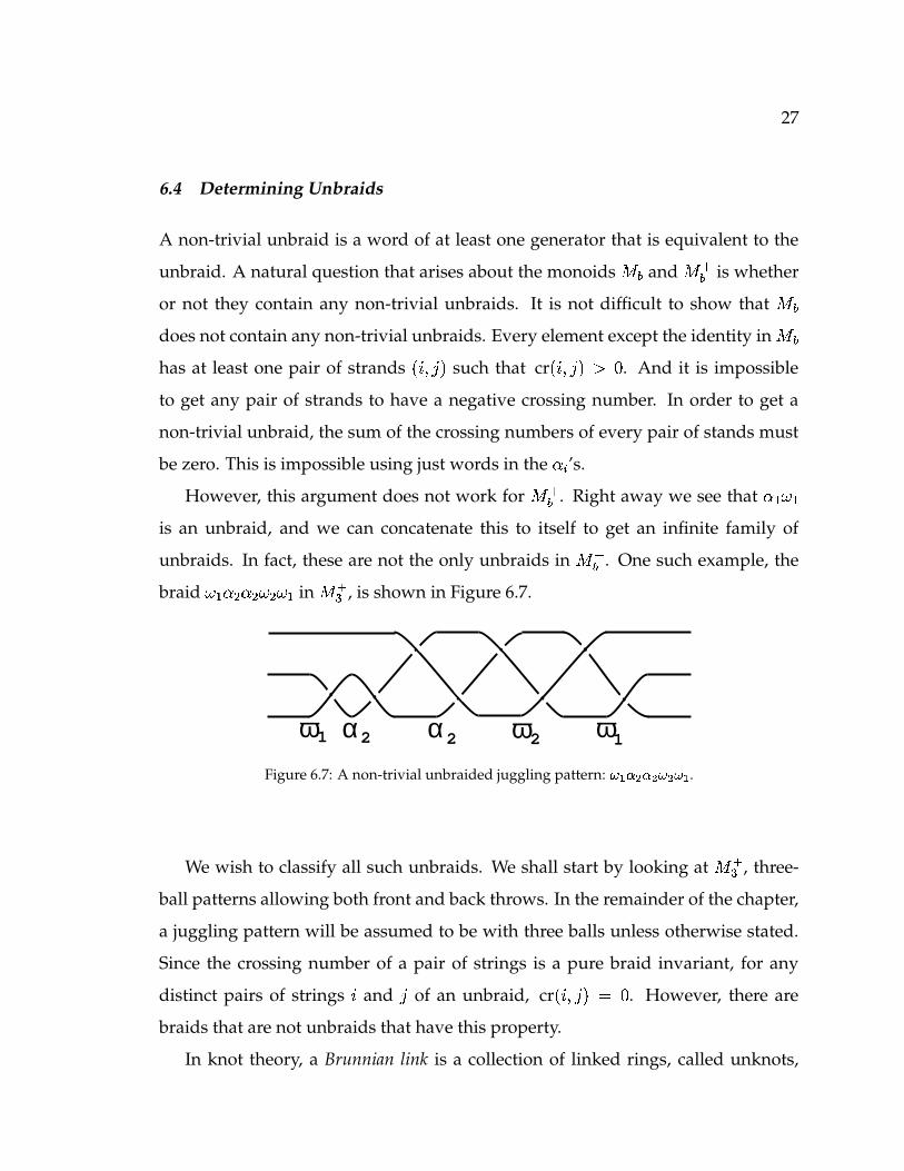
braid ")�'$(%!$�%'"(%'" � in � �� , is shown in Figure 6.7.

α α ω ωω1 122 2

Figure 6.7: A non-trivial unbraided juggling pattern: � �� .We wish to classify all such unbraids. We shall start by looking at � �

� , three-

ball patterns allowing both front and back throws. In the remainder of the chapter,

a juggling pattern will be assumed to be with three balls unless otherwise stated.

Since the crossing number of a pair of strings is a pure braid invariant, for any

distinct pairs of strings�

and�

of an unbraid, cr � � � � � �!� . However, there are

braids that are not unbraids that have this property.

In knot theory, a Brunnian link is a collection of linked rings, called unknots,

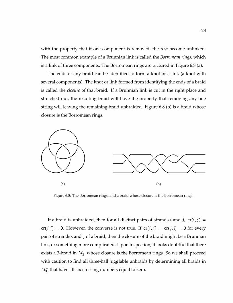
28

with the property that if one component is removed, the rest become unlinked.

The most common example of a Brunnian link is called the Borromean rings, which

is a link of three components. The Borromean rings are pictured in Figure 6.8 (a).

The ends of any braid can be identified to form a knot or a link (a knot with

several components). The knot or link formed from identifying the ends of a braid

is called the closure of that braid. If a Brunnian link is cut in the right place and

stretched out, the resulting braid will have the property that removing any one

string will leaving the remaining braid unbraided. Figure 6.8 (b) is a braid whose

closure is the Borromean rings.

(a) (b)

Figure 6.8: The Borromean rings, and a braid whose closure is the Borromean rings.

If a braid is unbraided, then for all distinct pairs of strands�

and�, cr � � � � � �

cr � � � � � � � . However, the converse is not true. If cr � � � � � � cr � � � � � � � for every

pair of strands�

and�

of a braid, then the closure of the braid might be a Brunnian

link, or something more complicated. Upon inspection, it looks doubtful that there

exists a 3-braid in � �� whose closure is the Borromean rings. So we shall proceed

with caution to find all three-ball jugglable unbraids by determining all braids in

� �� that have all six crossing numbers equal to zero.

29

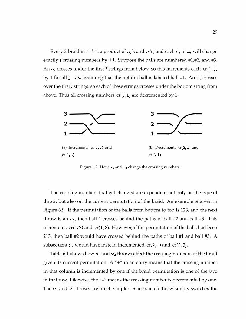
Every 3-braid in � �� is a product of $ � ’s and " � ’s, and each $ � or " � will change

exactly�

crossing numbers by� �

. Suppose the balls are numbered #1,#2, and #3.

An $ � crosses under the first�

strings from below, so this increments each cr � � � � �by 1 for all

� � �, assuming that the bottom ball is labeled ball #1. An "(� crosses

over the first�

strings, so each of these strings crosses under the bottom string from

above. Thus all crossing numbers cr � � � � � are decremented by 1.

1

2

3

(a) Increments cr �� and

cr ��

1

2

3

(b) Decrements cr � �� and

cr ��

Figure 6.9: How �� and �� change the crossing numbers.

The crossing numbers that get changed are dependent not only on the type of

throw, but also on the current permutation of the braid. An example is given in

Figure 6.9. If the permutation of the balls from bottom to top is 123, and the next

throw is an $(% , then ball 1 crosses behind the paths of ball #2 and ball #3. This

increments cr � � �!� � and cr � � � � � . However, if the permutation of the balls had been

213, then ball #2 would have crossed behind the paths of ball #1 and ball #3. A

subsequent $(% would have instead incremented cr � �� and cr � �� .Table 6.1 shows how $*% and "*% throws affect the crossing numbers of the braid

given its current permutation. A “+” in an entry means that the crossing number

in that column is incremented by one if the braid permutation is one of the two

in that row. Likewise, the “–” means the crossing number is decremented by one.

The $ � and " � throws are much simpler. Since such a throw simply switches the

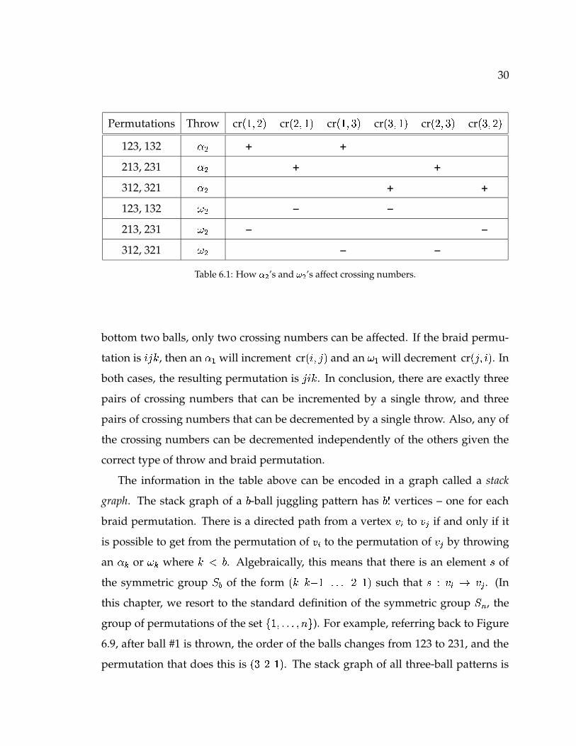
30

Permutations Throw cr � � �!� � cr � � � � � cr � � � � � cr � � � � � cr � � � � � cr � � �&� �123, 132 $(% + +

213, 231 $(% + +

312, 321 $(% + +

123, 132 " % – –

213, 231 " % – –

312, 321 " % – –

Table 6.1: How �� ’s and �� ’s affect crossing numbers.

bottom two balls, only two crossing numbers can be affected. If the braid permu-

tation is� � � , then an $ � will increment cr � � � � � and an ")� will decrement cr � � � � � . In

both cases, the resulting permutation is� � � . In conclusion, there are exactly three

pairs of crossing numbers that can be incremented by a single throw, and three

pairs of crossing numbers that can be decremented by a single throw. Also, any of

the crossing numbers can be decremented independently of the others given the

correct type of throw and braid permutation.

The information in the table above can be encoded in a graph called a stack

graph. The stack graph of a � -ball juggling pattern has �� vertices – one for each

braid permutation. There is a directed path from a vertex � � to � � if and only if it

is possible to get from the permutation of � � to the permutation of � � by throwing

an $(� or "*� where �� . Algebraically, this means that there is an element of

the symmetric group � � of the form � � � � � � � � � � � such that �� . (In

this chapter, we resort to the standard definition of the symmetric group � � , the

group of permutations of the set� � � � � � � � � ). For example, referring back to Figure

6.9, after ball #1 is thrown, the order of the balls changes from 123 to 231, and the

permutation that does this is � � � � � . The stack graph of all three-ball patterns is

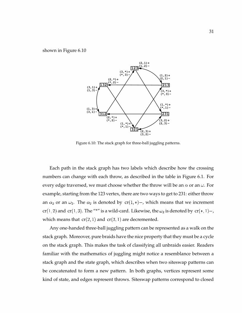
31

shown in Figure 6.10

123

321

132

312

213

231

(3,*)+(*,3)-

(2,*)+(*,2)-

(1,*)+(*,1)-

(3,*)+(*,3)-

(1,*)+(*,1)-

(2,*)+(*,2)-

(1,2)+(2,1)-

(2,1)+(1,2)-

(2,3)+(3,2)-

(3,2)+(2,3)-

(1,3)+(3,1)-

(3,1)+(1,3)-

Figure 6.10: The stack graph for three-ball juggling patterns.

Each path in the stack graph has two labels which describe how the crossing

numbers can change with each throw, as described in the table in Figure 6.1. For

every edge traversed, we must choose whether the throw will be an $ or an " . For

example, starting from the 123 vertex, there are two ways to get to 231: either throw

an $(% or an "*% . The $�% is denoted by cr � � �� , which means that we increment

cr � � �!� � and cr � � � � � . The “*” is a wild-card. Likewise, the " % is denoted by cr �� ,

which means that cr � � � � � and cr �� are decremented.

Any one-handed three-ball juggling pattern can be represented as a walk on the

stack graph. Moreover, pure braids have the nice property that they must be a cycle

on the stack graph. This makes the task of classifying all unbraids easier. Readers

familiar with the mathematics of juggling might notice a resemblance between a

stack graph and the state graph, which describes when two siteswap patterns can

be concatenated to form a new pattern. In both graphs, vertices represent some

kind of state, and edges represent throws. Siteswap patterns correspond to closed

32

loops on the state graph, whereas any path on the stack graph corresponds with a

siteswap pattern. However, state graphs and stack graphs describe two completely

different aspects of siteswap patterns. For a brief summary of state graphs, see

Appendix A. A great source for learning all about state graphs is [9].

The stack graph displays a good deal of symmetry. There are two types of

edges: each vertex has one “long” edge, corresponding with an $ % or "(% , going

into it and one going out of it. Also, each vertex has one “short” edge, correspond-

ing with an $ � or ")� , going into it and one short edge leaving. Next we will present

several ways to set up a system of equations whose solutions will describe all un-

braids.

6.4.1 Setting the crossing numbers to zero.

Without loss of generality, assume that any three ball juggling pattern begins with

the permutation 123. If we keep a running total of the sum of all six crossing

numbers, then unbraids will be cycles such that all six crossing numbers are zero.

There are six pairs of crossing numbers that can be changed with a single throw,

as well as all six individual crossing numbers that can be changed independently.

Thus there are twelve possible non-empty subsets of

�cr � � �&� � � cr � � � � � � cr � � � � � � cr � � � � � � cr � � � � � � cr � � �!� � �

that can be changed by a single throw. An unbraid has the restriction that each of

the crossing numbers is zero. This gives us a system of six equations on twelve

33

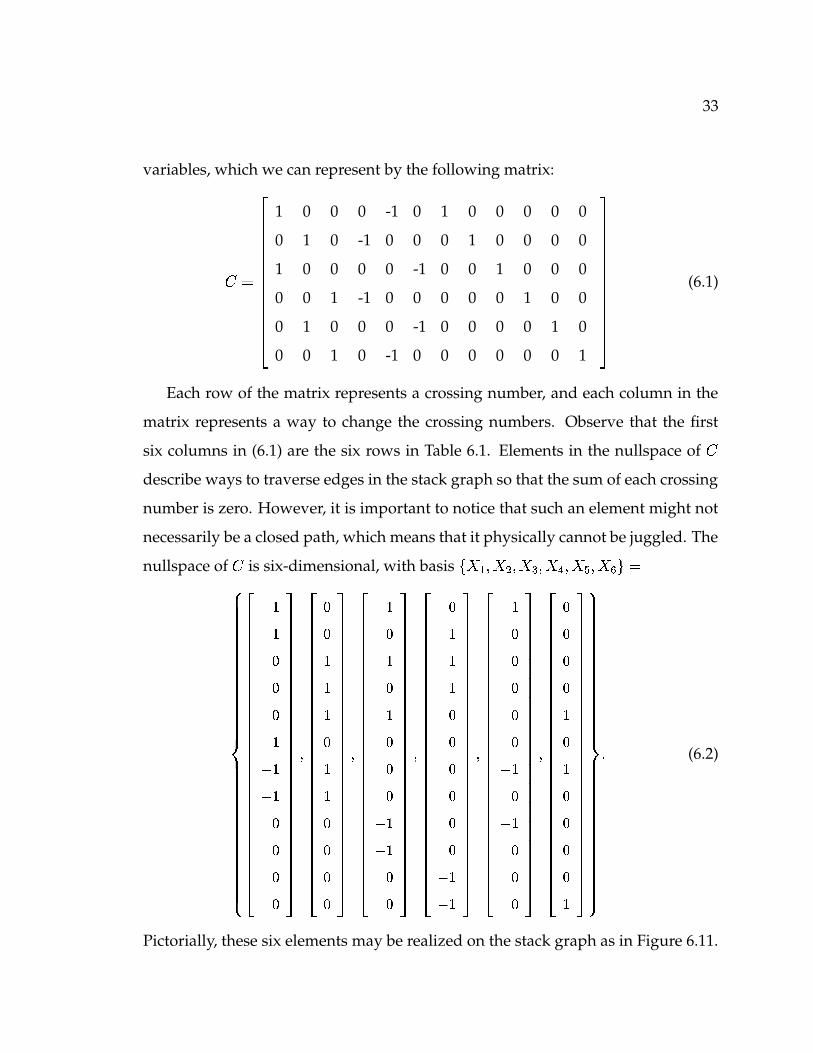
variables, which we can represent by the following matrix:

� �

��

1 0 0 0 -1 0 1 0 0 0 0 0

0 1 0 -1 0 0 0 1 0 0 0 0

1 0 0 0 0 -1 0 0 1 0 0 0

0 0 1 -1 0 0 0 0 0 1 0 0

0 1 0 0 0 -1 0 0 0 0 1 0

0 0 1 0 -1 0 0 0 0 0 0 1

��

(6.1)

Each row of the matrix represents a crossing number, and each column in the

matrix represents a way to change the crossing numbers. Observe that the first

six columns in (6.1) are the six rows in Table 6.1. Elements in the nullspace of�

describe ways to traverse edges in the stack graph so that the sum of each crossing

number is zero. However, it is important to notice that such an element might not

necessarily be a closed path, which means that it physically cannot be juggled. The

nullspace of�

is six-dimensional, with basis� +,� �'+ % ��+ � ��+�� + ��+� � ��

��

��

� ��

�

��

��

� ��

�

��

� � � � ��

� ��

�

��

��

� ��

�

��

� � � � �

� ��

�

��

� � �

� ��

� � �

� (6.2)

Pictorially, these six elements may be realized on the stack graph as in Figure 6.11.

34

123

321

132

312

213

231

(2,1)-(1,2)-

(*,3)-

(2,*)+

(1,*)+

123

321

132

312

213

231

(1,2)+(2,1)+

(*,1)-

(*,2)-

(3,*)+

X2

123

321

132

312

213

231

(1,*)+

(*,2)-

(3,*)+

(3,1)-

(1,3)-X3

123

321

132

312

213

231

(*,1)-

(2,*)+

(3,*)+

(2,3)-

X4

(3,2)-

123

321

132

312

213

231

(1,2)-

(1,*)+

(1,3)- X5

123

321

132

312

213

231

(3,2)+(*,2)-

X6

(1,2)+

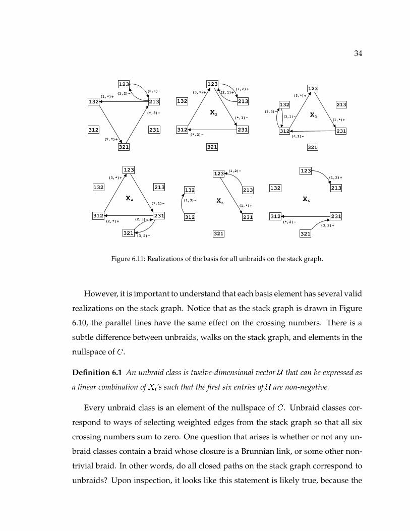
Figure 6.11: Realizations of the basis for all unbraids on the stack graph.

However, it is important to understand that each basis element has several valid

realizations on the stack graph. Notice that as the stack graph is drawn in Figure

6.10, the parallel lines have the same effect on the crossing numbers. There is a

subtle difference between unbraids, walks on the stack graph, and elements in the

nullspace of�

.

Definition 6.1 An unbraid class is twelve-dimensional vector � that can be expressed as

a linear combination of + � ’s such that the first six entries of � are non-negative.

Every unbraid class is an element of the nullspace of�

. Unbraid classes cor-

respond to ways of selecting weighted edges from the stack graph so that all six

crossing numbers sum to zero. One question that arises is whether or not any un-

braid classes contain a braid whose closure is a Brunnian link, or some other non-

trivial braid. In other words, do all closed paths on the stack graph correspond to

unbraids? Upon inspection, it looks like this statement is likely true, because the

35

braid in 6.8(b) does not appear to be jugglable, and because + � ��+ % ��+ � , and + � are

all unbraids. However, we cannot rule out the possibility.

It is important to understand that unbraid classes do not specify the order

that the edges are traversed, so an unbraid class can correspond to many un-

braids (or possibly, braids with Brunnian link closures). For example, suppose that

� � + � � + %�� + � . Starting at vertex 123 in the stack graph, one possible unbraid

of � is to traverse + � ��+ % , and + � in that order as shown in Figure 6.11. Another

possibility is + � ��+ � ��+ % . Still, there are more complicated ways. Notice that there

are two potential starting directions for + % as it is depicted in Figure 6.11 when

starting at vertex 123. It is even possible to insert one of the + � ’s before finishing

traversing another. For example, traverse + % and upon reaching the 312 vertex,

before completing the cycle, start traversing + � , but upon reaching the 123 vertex,

traverse + � . Then finish + � , and then finish + % . These are all realizations of the

unbraid class + � � + % � + � . There are also realizations of unbraid classes that do

not correspond with paths on the stack graph.

Definition 6.1 A walk of an unbraid class � is a path on the stack graph that is a realiza-

tion of � .

A walk of an unbraid class is a cycle on the stack graph. Every walk gives rise

to precisely one braid.

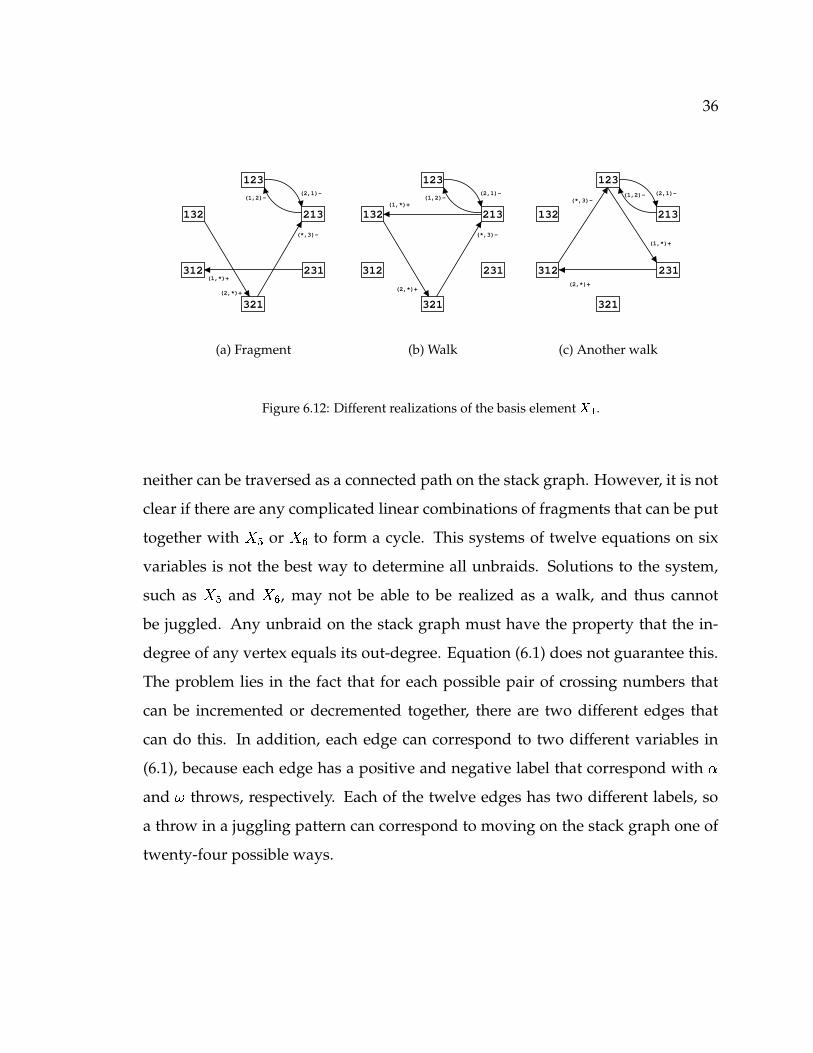
Definition 6.2 A fragment of an unbraid class � is a realization of � that is not a walk.

A walk is not a fragment and a fragment is not a walk. Moreover, every realiza-

tion of an unbraid class on the stack graph is either a walk or a fragment. A walk

can be juggled but a fragment cannot. Figure 6.12 shows + � realized three different

ways. The first one is a fragment and the last two are walks.

The basis element + � can be realized as the braid " �'$�%&$�%�"*%�")� , which is the

unbraid shown in Figure 6.7. Every realization of + and + � are fragments because

36

123

321

132

312

213

231

(2,1)-(1,2)-

(*,3)-

(2,*)+

(1,*)+

(a) Fragment

123

321

132

312

213

231

(2,1)-(1,2)-

(*,3)-

(2,*)+

(1,*)+

(b) Walk

123

321

132

312

213

231

(2,1)-(1,2)-(*,3)-

(2,*)+

(1,*)+

(c) Another walk

Figure 6.12: Different realizations of the basis element � � .neither can be traversed as a connected path on the stack graph. However, it is not

clear if there are any complicated linear combinations of fragments that can be put

together with + or + � to form a cycle. This systems of twelve equations on six

variables is not the best way to determine all unbraids. Solutions to the system,

such as + and +� , may not be able to be realized as a walk, and thus cannot

be juggled. Any unbraid on the stack graph must have the property that the in-

degree of any vertex equals its out-degree. Equation (6.1) does not guarantee this.

The problem lies in the fact that for each possible pair of crossing numbers that

can be incremented or decremented together, there are two different edges that

can do this. In addition, each edge can correspond to two different variables in

(6.1), because each edge has a positive and negative label that correspond with $and " throws, respectively. Each of the twelve edges has two different labels, so

a throw in a juggling pattern can correspond to moving on the stack graph one of

twenty-four possible ways.

37

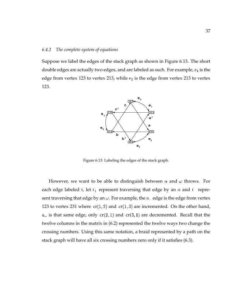
6.4.2 The complete system of equations

Suppose we label the edges of the stack graph as shown in Figure 6.13. The short

double edges are actually two edges, and are labeled as such. For example, � is the

edge from vertex 123 to vertex 213, while % is the edge from vertex 213 to vertex

123.

123

321

132

312

213

231

a

b

c

a’

b’

c’e

e

e

e

e

e

1

2

3

4

5

6

Figure 6.13: Labeling the edges of the stack graph.

However, we want to be able to distinguish between $ and " throws. For

each edge labeled�, let

� � represent traversing that edge by an $ and� �

repre-

sent traversing that edge by an " . For example, the �� edge is the edge from vertex

123 to vertex 231 where cr � � �!� � and cr � � � � � are incremented. On the other hand,

� � is that same edge, only cr � � � � � and cr � � � � � are decremented. Recall that the

twelve columns in the matrix in (6.2) represented the twelve ways two change the

crossing numbers. Using this same notation, a braid represented by a path on the

stack graph will have all six crossing numbers zero only if it satisfies (6.3).

38

��

��

� ��

��

� ��

��

� ��

��

� ��

��

� ��

��

� ��

� ��

��

�

� ��

��

�

� ��

��

�

� ��

��

�

� ��

��

�

� ��

��

�

� ��

��

� ��

(6.3)

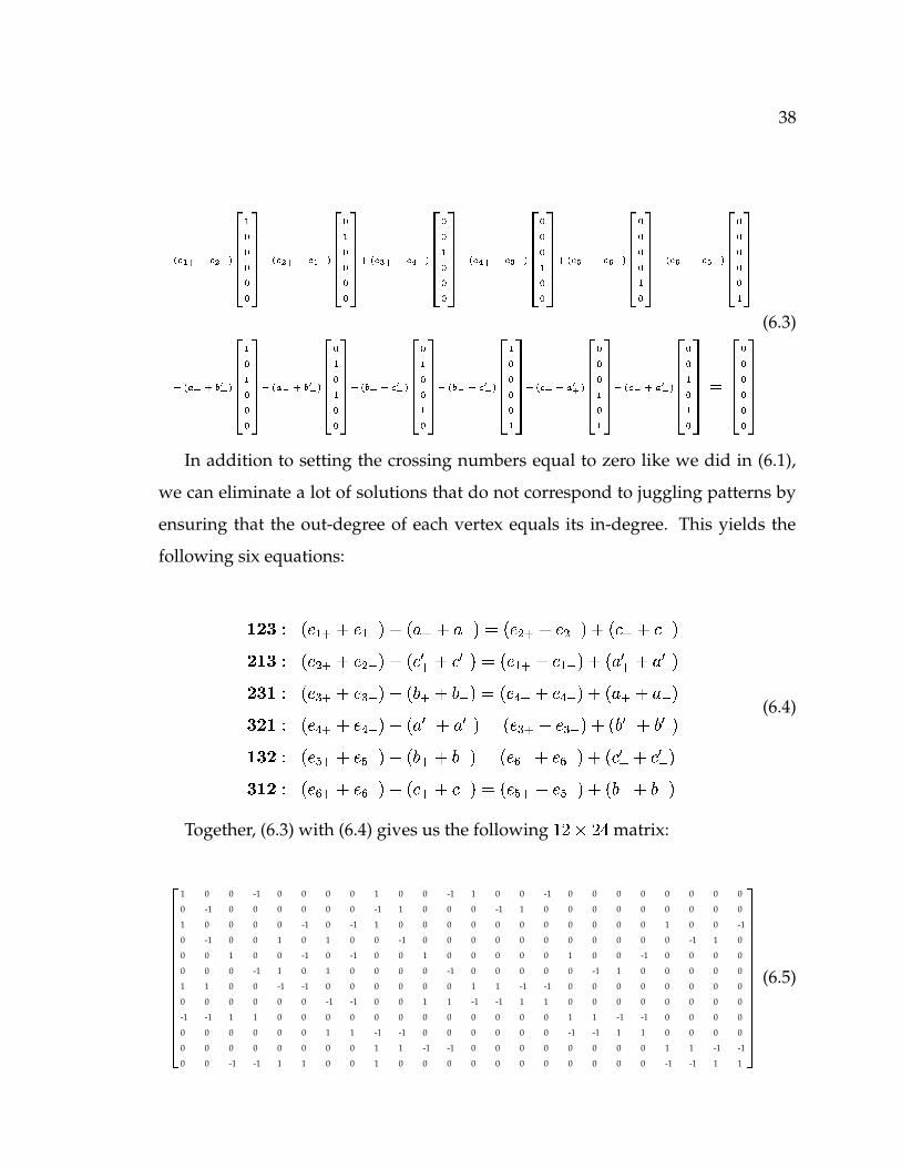
In addition to setting the crossing numbers equal to zero like we did in (6.1),

we can eliminate a lot of solutions that do not correspond to juggling patterns by

ensuring that the out-degree of each vertex equals its in-degree. This yields the

following six equations:

� �"! � � � � � � � � � � � � � � � �)� � % � � % � � � �#�� $#� �

�%�&! � � % � � % � � � ��# � � �'#�� "!(� � � � � � �

� � � � � � �� '� � � � � � � �� !)�%� � � �� )� � � � � �

� � � � �� &!)� � � � � � � � � � � �� #�� '#�� !(� � � � � � � � � � � ��#�� '#

� � � � � � � � � � � � � � � �

(6.4)

Together, (6.3) with (6.4) gives us the following� �+*�� matrix:

��

1 0 0 -1 0 0 0 0 1 0 0 -1 1 0 0 -1 0 0 0 0 0 0 0 0

0 -1 0 0 0 0 0 0 -1 1 0 0 0 -1 1 0 0 0 0 0 0 0 0 0

1 0 0 0 0 -1 0 -1 1 0 0 0 0 0 0 0 0 0 0 0 1 0 0 -1

0 -1 0 0 1 0 1 0 0 -1 0 0 0 0 0 0 0 0 0 0 0 -1 1 0

0 0 1 0 0 -1 0 -1 0 0 1 0 0 0 0 0 1 0 0 -1 0 0 0 0

0 0 0 -1 1 0 1 0 0 0 0 -1 0 0 0 0 0 -1 1 0 0 0 0 0

1 1 0 0 -1 -1 0 0 0 0 0 0 1 1 -1 -1 0 0 0 0 0 0 0 0

0 0 0 0 0 0 -1 -1 0 0 1 1 -1 -1 1 1 0 0 0 0 0 0 0 0

-1 -1 1 1 0 0 0 0 0 0 0 0 0 0 0 0 1 1 -1 -1 0 0 0 0

0 0 0 0 0 0 1 1 -1 -1 0 0 0 0 0 0 -1 -1 1 1 0 0 0 0

0 0 0 0 0 0 0 0 1 1 -1 -1 0 0 0 0 0 0 0 0 1 1 -1 -1

0 0 -1 -1 1 1 0 0 1 0 0 0 0 0 0 0 0 0 0 0 -1 -1 1 1

� ��

(6.5)

39

The nullspace of (6.5) is thirteen-dimensional, and vectors in the nullspace de-

scribe every possible unbraid that is a cycle. However, since traversing an edge a

negative number of times has no physical meaning, a vector in the nullspace can

only be physically realized as an unbraid if all of its entries are non-negative. It is

inconvenient to have a basis of unbraids consisting of thirteen � � * � vectors, most

of which are not even realizable juggling patterns.

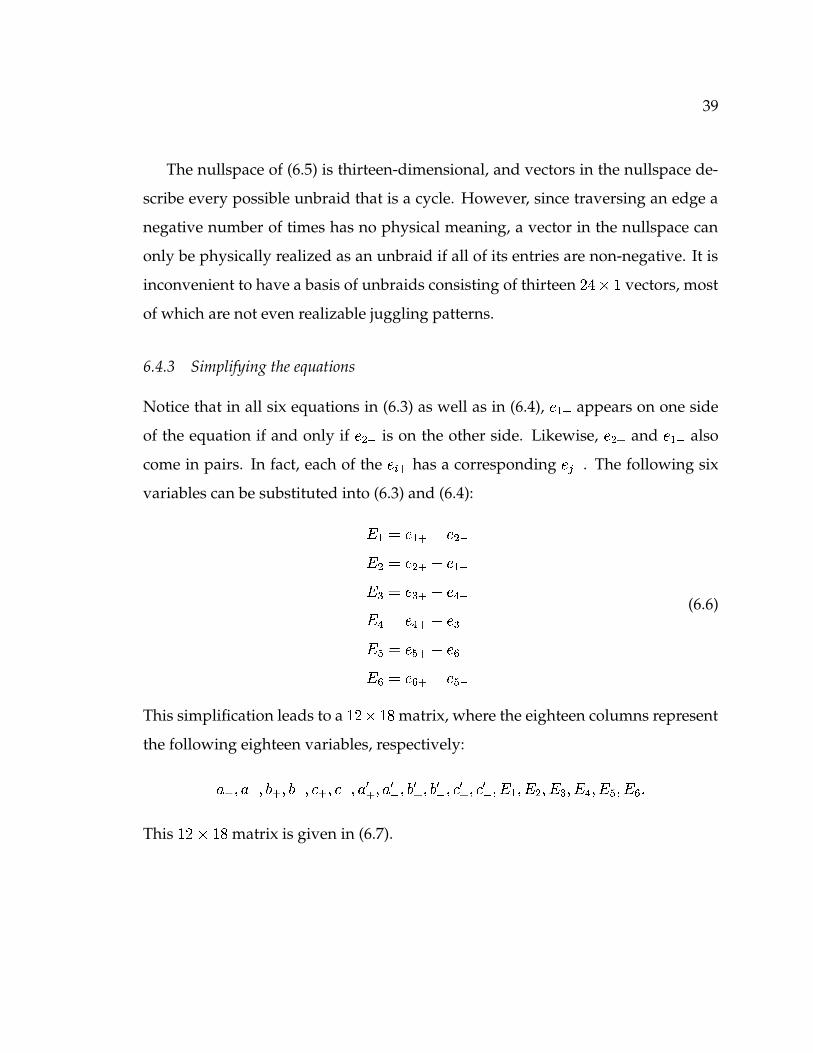
6.4.3 Simplifying the equations

Notice that in all six equations in (6.3) as well as in (6.4), � � appears on one side

of the equation if and only if % � is on the other side. Likewise, % � and � � also

come in pairs. In fact, each of the � � has a corresponding � � . The following six

variables can be substituted into (6.3) and (6.4):

� � � � � � % �� % � % � � � ��

� � � ��

� � � �'� � ��

� � � � � ��

(6.6)

This simplification leads to a� � * �� matrix, where the eighteen columns represent

the following eighteen variables, respectively:

�� #�� # � � � � � �� # � � � # � � � � � � � % � � � ��

This� �+* �� matrix is given in (6.7).

40

��

1 0 0 -1 0 0 0 0 1 0 0 -1 1 0 0 0 0 0

0 -1 0 0 0 0 0 0 -1 1 0 0 0 1 0 0 0 0

1 0 0 0 0 -1 0 -1 1 0 0 0 0 0 0 0 1 0

0 -1 0 0 1 0 1 0 0 -1 0 0 0 0 0 0 0 1

0 0 1 0 0 -1 0 -1 0 0 1 0 0 0 1 0 0 0

0 0 0 -1 1 0 1 0 0 0 0 -1 0 0 0 1 0 0

1 1 0 0 -1 -1 0 0 0 0 0 0 1 -1 0 0 0 0

0 0 0 0 0 0 -1 -1 0 0 1 1 -1 1 0 0 0 0

-1 -1 1 1 0 0 0 0 0 0 0 0 0 0 1 -1 0 0

0 0 0 0 0 0 1 1 -1 -1 0 0 0 0 -1 1 0 0

0 0 0 0 0 0 0 0 1 1 -1 -1 0 0 0 0 1 -1

0 0 -1 -1 1 1 0 0 1 0 0 0 0 0 0 0 -1 1

� ��

(6.7)

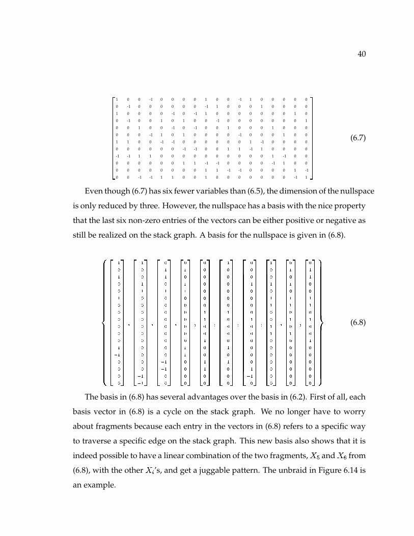
Even though (6.7) has six fewer variables than (6.5), the dimension of the nullspace

is only reduced by three. However, the nullspace has a basis with the nice property

that the last six non-zero entries of the vectors can be either positive or negative as

still be realized on the stack graph. A basis for the nullspace is given in (6.8).

� � �

��

�

�

�

�

�

��

�

��

�

�

�

�

�

��

�

��

�

�

�

�

�

��

�

��

�

�

�

�

�

��

�

��

�

�

�

�

�

��

�

��

�

�

�

�

��

�

��

�

�

�

�

��

�

��

�

�

�

�

�

�

��

�

��

�

�

�

�

�

�

��

�

��

�

�

�

�

�

�

��

� � �

(6.8)

The basis in (6.8) has several advantages over the basis in (6.2). First of all, each

basis vector in (6.8) is a cycle on the stack graph. We no longer have to worry

about fragments because each entry in the vectors in (6.8) refers to a specific way

to traverse a specific edge on the stack graph. This new basis also shows that it is

indeed possible to have a linear combination of the two fragments, + and + � from

(6.8), with the other + � ’s, and get a juggable pattern. The unbraid in Figure 6.14 is

an example.

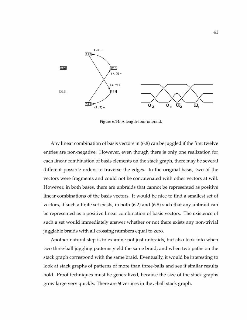
41

123

321

132

312

213

231

(*,3)-

(1,*)+

(1,2)-

(2,3)+ α α ω ω122 2

Figure 6.14: A length-four unbraid.

Any linear combination of basis vectors in (6.8) can be juggled if the first twelve

entries are non-negative. However, even though there is only one realization for

each linear combination of basis elements on the stack graph, there may be several

different possible orders to traverse the edges. In the original basis, two of the

vectors were fragments and could not be concatenated with other vectors at will.

However, in both bases, there are unbraids that cannot be represented as positive

linear combinations of the basis vectors. It would be nice to find a smallest set of

vectors, if such a finite set exists, in both (6.2) and (6.8) such that any unbraid can

be represented as a positive linear combination of basis vectors. The existence of

such a set would immediately answer whether or not there exists any non-trivial

jugglable braids with all crossing numbers equal to zero.

Another natural step is to examine not just unbraids, but also look into when

two three-ball juggling patterns yield the same braid, and when two paths on the

stack graph correspond with the same braid. Eventually, it would be interesting to

look at stack graphs of patterns of more than three-balls and see if similar results

hold. Proof techniques must be generalized, because the size of the stack graphs

grow large very quickly. There are �� vertices in the � -ball stack graph.

42

6.5 Adding More Balls

Thus far, we have not examined the stack graphs of patterns with more than three

balls because the size of the graph grows very quickly. A good way to understand

a larger stack graph is to collapse it into a smaller graph. For any stack graph, iden-

tify two vertices if they have the same top ball in their permutation, and remove

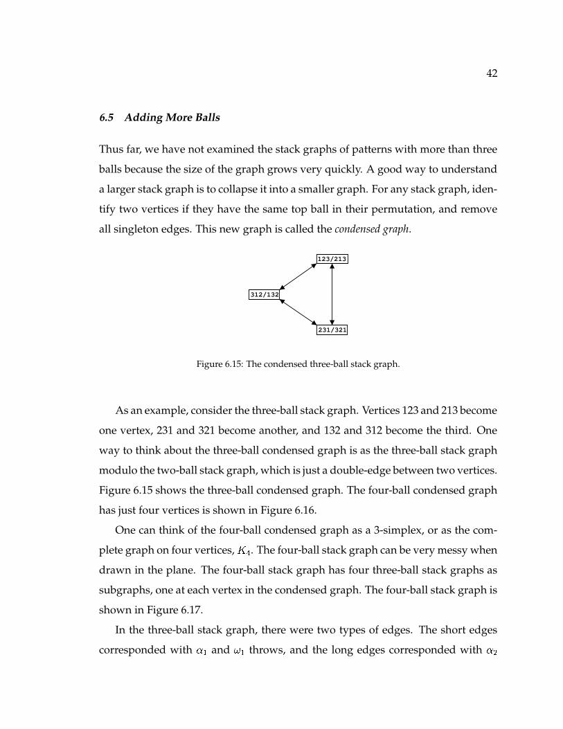
all singleton edges. This new graph is called the condensed graph.

123/213

231/321

312/132

Figure 6.15: The condensed three-ball stack graph.

As an example, consider the three-ball stack graph. Vertices 123 and 213 become

one vertex, 231 and 321 become another, and 132 and 312 become the third. One

way to think about the three-ball condensed graph is as the three-ball stack graph

modulo the two-ball stack graph, which is just a double-edge between two vertices.

Figure 6.15 shows the three-ball condensed graph. The four-ball condensed graph

has just four vertices is shown in Figure 6.16.

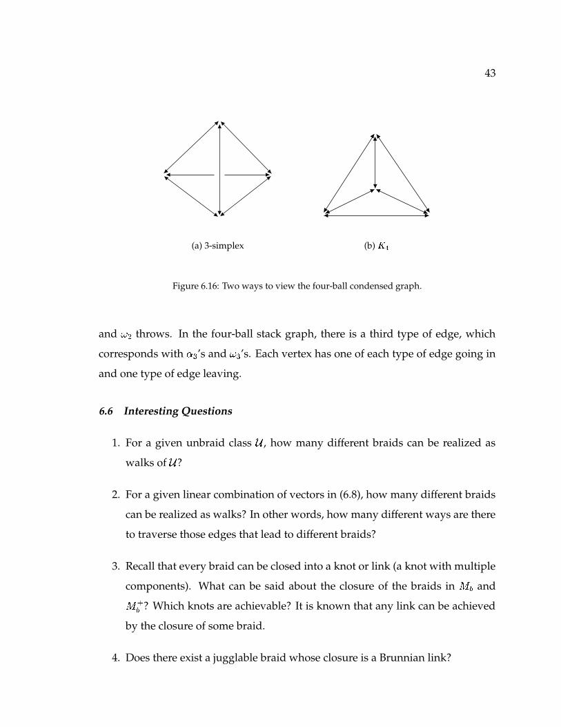
One can think of the four-ball condensed graph as a 3-simplex, or as the com-

plete graph on four vertices, � � . The four-ball stack graph can be very messy when

drawn in the plane. The four-ball stack graph has four three-ball stack graphs as

subgraphs, one at each vertex in the condensed graph. The four-ball stack graph is

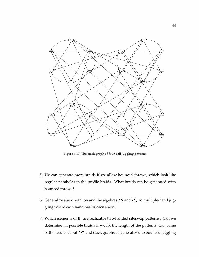
shown in Figure 6.17.

In the three-ball stack graph, there were two types of edges. The short edges

corresponded with $ � and ")� throws, and the long edges corresponded with $*%

43

(a) 3-simplex (b) ��

Figure 6.16: Two ways to view the four-ball condensed graph.

and "*% throws. In the four-ball stack graph, there is a third type of edge, which

corresponds with $ � ’s and " � ’s. Each vertex has one of each type of edge going in

and one type of edge leaving.


1. For a given unbraid class � , how many different braids can be realized as

walks of � ?

2. For a given linear combination of vectors in (6.8), how many different braids

can be realized as walks? In other words, how many different ways are there

to traverse those edges that lead to different braids?

3. Recall that every braid can be closed into a knot or link (a knot with multiple

components). What can be said about the closure of the braids in � � and

� ��

? Which knots are achievable? It is known that any link can be achieved

by the closure of some braid.

4. Does there exist a jugglable braid whose closure is a Brunnian link?

44

1234

2341

4123

3412

1342

3421

2134

4213

2314

3142

1423

4231

3214

2143

1432

4321

2431

4312

3124

1243

1324 2413

3241

4132

Figure 6.17: The stack graph of four-ball juggling patterns.

5. We can generate more braids if we allow bounced throws, which look like

regular parabolas in the profile braids. What braids can be generated with

bounced throws?

6. Generalize stack notation and the algebras � � and � ��

to multiple-hand jug-

gling where each hand has its own stack.

7. Which elements of B � are realizable two-handed siteswap patterns? Can we

determine all possible braids if we fix the length of the pattern? Can some

of the results about � ��

and stack graphs be generalized to bounced juggling

45

patterns?

8. We call two � -ball juggling patterns homotopic if they yield the same braid

in B � . For a given � , how many distinct juggling patterns are there up to

homotopy? Recall that we have an upper bound for this number, not an

exact value.

9. Define the writhe of a braid to be the sum of the exponents of the � � ’s. The

writhe basically measures how much the braid is twisting. If � is a two-

handed siteswap pattern of odd period, then � � � � � �� . If � � � � � � � � �for some two-handed siteswap pattern � , then must � have odd period?

Appendix A

Appendix

A.1 State Graphs

Suppose we are juggling a siteswap pattern, and want to know which throws, no

higher than a certain digit, can be thrown next beat. State graphs can answer this.

Set a maximum throw height, � . At any point while juggling, we look at the next

� beats and write a 0 if no ball will land and a 1 if a ball will land. For example,

suppose one wants to know what can be thrown after the 1 in the four-ball pattern

561, and because of a low ceiling, the highest throw must be no more than a 7. In

this case, consider the next seven beats.

� � � �� x x x x

The x’s denote beats when the four balls will land. We write this as

� � � � � ��

The first digit of this sequence represents the next throw. Because two balls can’t

land on the same beat, the next throw cannot be a 1, 2, or 4. However, a 3, 5, 6, or 7

will work. Suppose we throw a 3. Then our pattern becomes

� � � �� x x x x �

which gives rise to the binary string

� � � � ��

47

In the example with four balls and maximum height 7, there are 35 possible bi-

nary strings. We can construct a graph where each vertex represents a legal binary

string, and there is a directed edge from vertex � � to � � if and only if it is possible

to go from the state � � to � � by a single throw. That edge is labeled with the height

of the throw required to go from � � to � � . In the above example, there would be a

directed edge labeled with a 6, from the 1110100 vertex to the 1111000 vertex. Such

a graph is called a state graph. State graphs are discussed extensively in [9]. They

have the nice property that any possible siteswap pattern given constraints of the

number of balls and the maximum throw height, corresponds to some path on the

state graph. Conversely, for any path of the state graph, the string the digits of the

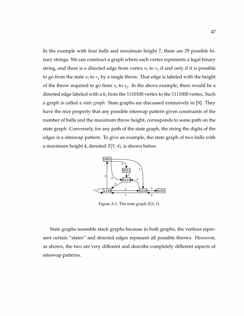
edges is a siteswap pattern. To give an example, the state graph of two balls with

a maximum height 4, denoted �� , is shown below.

1100

1001

1010

0011

0101

0110

4

1

0

0

24

2 3

1

3

0

4

Figure A.1: The state graph � � �� .State graphs resemble stack graphs because in both graphs, the vertices repre-

sent certain “states” and directed edges represent all possible throws. However,

as shown, the two are very different and describe completely different aspects of

siteswap patterns.

48

(b,n) 1 2 3 4 5 6 7 8 9 10

2 1 1 1 1 1 1 1 1 1 1

3 1 2 4 7 13 22 40 70 126 225

4 1 3 9 24 66 173 467 1247 3375 9156

5 1 4 16 58 214 768 2796 10146 37082 135956

6 1 5 25 115 535 2445 11265 51855 239735 1111229

Table A.1: Equation (A.1) evaluated for small � and �

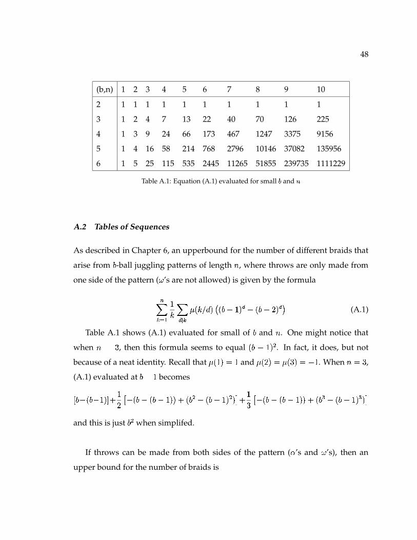
A.2 Tables of Sequences

As described in Chapter 6, an upperbound for the number of different braids that

arise from � -ball juggling patterns of length � , where throws are only made from

one side of the pattern ( " ’s are not allowed) is given by the formula

��

��

� �(A.1)

Table A.1 shows (A.1) evaluated for small of � and � . One might notice that

when � � � , then this formula seems to equal � � � � � % . In fact, it does, but not

because of a neat identity. Recall that � � � � � � and � � � �)� � � � � � � �. When �� ,

(A.1) evaluated at � �� becomes

� � � � � ��

� � � � � � � �� % � � � � � � % � � ��

� � � � � � � � � ��

and this is just � % when simplifed.

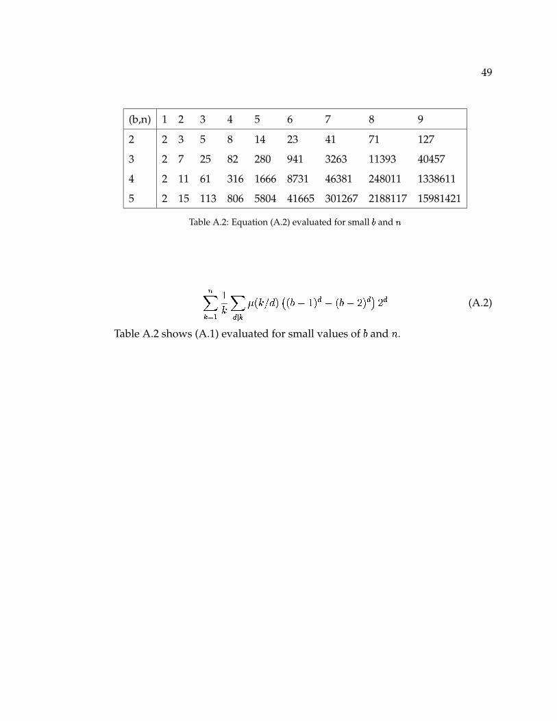
If throws can be made from both sides of the pattern ( $ ’s and " ’s), then an

upper bound for the number of braids is

49

(b,n) 1 2 3 4 5 6 7 8 9

2 2 3 5 8 14 23 41 71 127

3 2 7 25 82 280 941 3263 11393 40457

4 2 11 61 316 1666 8731 46381 248011 1338611

5 2 15 113 806 5804 41665 301267 2188117 15981421

Table A.2: Equation (A.2) evaluated for small � and �

��

��

��

(A.2)

Table A.2 shows (A.1) evaluated for small values of � and � .

Bibliography

[1] C. Adams. The Knot Book. W.H.Freeman, 1994.

[2] B. Tiemann B. Magnusson. The physics of juggling. Physics Teacher, 27:584–

589, 1989.

[3] J. Buhler, D. Eisenbud, R. Graham, and C. Wright. Juggling drops and de-

scents. American Mathematical Monthly, 101(6):507–519, 1994.

[4] The juggling information service. Available online at

http://www.juggling.org.

[5] B.I. Kurpita K. Murasugi. A Study of Braids. Kluwer Academic Publishers,

1999.

[6] J. Kalvin. Optimal juggling. Published online at

http://www.juggling.org/papers, 1996.

[7] J. Kalvin. The human limits. Published online at

http://www.juggling.org/papers, 1997.

[8] D. Margalit, N. Picciotto, and S. Babineau J. Llobrera. Topology and juggling.

Published online at

http://www.brown.edu/Students/OHJC/topology/index.html,

2002.

[9] B. Polster. The Mathematics of Juggling. Springer-Verlag, 2003.

51

[10] M.A. Readdy R. Ehrenborg. Juggling and applications to � -analogues. Alge-

braic Combinatorics in Discrete Mathematics, 157:107–125, 1996.

[11] rec.juggling newsgroup. The archives of the newsgroup can be found at

http://www.juggling.org.

[12] N.J.A. Sloane. The on-line encyclopedia of integer sequences. Available online

at http://www.research.att.com/njas/sequences/, 2002.

[13] R.P. Stanley. Enumerative Combinatorics. Cambridge University Press, 2001.

Documents

Braids and Juggling Patterns Matthew Macauley Michael Orrison