Embed Size (px)
Citation preview
Report of the Inquiry into the 2015
British general election opinion polls
Professor Patrick Sturgis, University of Southampton
Dr Nick Baker, Quadrangle
Dr Mario Callegaro, Google
Dr Stephen Fisher, University of Oxford
Professor Jane Green, University of Manchester
Professor Will Jennings, University of Southampton
Dr Jouni Kuha, London School of Economics and Political Science
Dr Ben Lauderdale, London School of Economics and Political Science
Dr Patten Smith, Ipsos-MORI

i
Published by the British Polling Council and the Market Research Society, London, March 2016. How to cite this report: Sturgis, P. Baker, N. Callegaro, M. Fisher, S. Green, J. Jennings, W. Kuha, J. Lauderdale, B. and Smith, P. (2016) Report of the Inquiry into the 2015 British general election opinion polls, London: Market Research Society and British Polling Council.
ii
Table of Contents
Acknowledgements ....................................................................................................................................... 1
Foreword ........................................................................................................................................................... 2
Executive Summary....................................................................................................................................... 4
1. Introduction ............................................................................................................................................. 7
2. How the Inquiry was conducted ...................................................................................................... 9
3. Assessing the accuracy of the pre-election poll estimates .................................................. 11
4. Historical and comparative context ............................................................................................. 15
4.1 International context .................................................................................................................. 20
5. The methodology of opinion polls ................................................................................................ 22
5.1 Deriving the sample of voters and estimating voting intention ................................. 23
Online data collection ....................................................................................................................... 25
Telephone data collection ............................................................................................................... 25
5.2 When quota sampling produces inaccurate estimates: an example ........................ 26
6. Assessment of putative causes of the polling error................................................................ 29
6.1 Postal voting ................................................................................................................................... 29
6.2 Overseas voters ............................................................................................................................. 30
6.3 Voter registration ......................................................................................................................... 31
6.4 Question wording and framing ............................................................................................... 31
6.5 Late swing ....................................................................................................................................... 34
6.6 Deliberate misreporting ............................................................................................................ 39
6.7 Turnout weighting ....................................................................................................................... 42
How accurate were the turnout weights? ................................................................................. 42
How did turnout weights affect the published vote intention figures? ......................... 44
‘Lazy-Labour’ and differential turnout misreporting ........................................................... 46
6.8 Unrepresentative samples ........................................................................................................ 47
6.9 Mode of interview ........................................................................................................................ 58
7. Herding .................................................................................................................................................... 62
8. Conclusions and recommendations ............................................................................................. 69
9. References .............................................................................................................................................. 80
10. Appendices .......................................................................................................................................... 83
Appendix 1: Methodological details of Polls Considered by the Inquiry ........................... 84
Appendix 2: Polls in Scotland undertaken in the final week of the campaign ................. 86

iii
Appendix 3: Final polls, 1945-2010 ................................................................................................. 87
Appendix 4: Methodology of sampling and estimation in election polls ........................ 103
Appendix 5: Wording and ordering of vote intention questions ....................................... 106
Appendix 6: Technical details of herding analysis .................................................................. 110
Appendix 7: Inquiry Terms of Reference .................................................................................... 114
Appendix 8: Conservative lead estimates by weighting cells ............................................. 115

iv
Tables
Table 1. Final Polls, Published Estimates ............................................................................................ 12
Figures
Figure 1. Two month moving average poll estimates 2010-2015 ............................................ 13
Figure 2. Average Mean Absolute Error, Conservatives and Labour ....................................... 16
Figure 3. Minimum Mean Absolute Error, Conservative and Labour ...................................... 17
Figure 4. Net error in poll estimates of Conservative vote shares ............................................ 18
Figure 5. Net error in poll estimates of Labour vote shares ........................................................ 19
Figure 6. Net error in poll estimates of the Conservative lead over Labour ......................... 20
Figure 7. Conservative lead for BES/BSA at different call numbers ........................................ 27
Figure 8. Conservative lead, pre-election polls & re-contact surveys ..................................... 36
Figure 9. Reported turnout in re-contact surveys by turnout weight ..................................... 43
Figure 10. Conservative lead under alternative turnout probabilities ................................... 45
Figure 11. Reported vote and vote intention: BES, BSA, polls .................................................... 49
Figure 12. Conservative lead by age group, polls v BES/BSA ..................................................... 52
Figure 13. Conservative lead by GB region, polls v election results ......................................... 52
Figure 14. Continuous age distribution for 65+ age band (polls v census) ........................... 55
Figure 15. Banded age distribution for postal voters (polls v BES) ......................................... 56
Figure 16. Self-reported 2010 turnout by age band (polls v BES) ............................................ 57
Figure 17. Conservative lead 2010-2015 by interview mode of polls .................................... 60
Figure 18. Mode Difference in Conservative lead, polls 2010-2015 ........................................ 61
Figure 19. Assumed & observed variance in poll estimates, Conservative lead ................. 65
Figure 20. Conservative lead in final polls, alternative weighting procedures.................... 66
Figure 21. Conservative lead: actual v harmonised adjustment procedures ....................... 67

1
Acknowledgements
We are grateful to the British Polling Council (BPC) and the Market Research Society
(MRS) for providing us with the opportunity to undertake this important and
interesting work. We also extend our thanks to the nine member organisations of the
BPC who have been cooperative throughout, providing all data requested, as well as
supplementary information in a timely manner. It should be noted that this is in stark
contrast to experience in the United States, where slow responses and partial non-
cooperation by pollsters stymied the progress of the American Association of Public
Opinion Research’s (AAPOR) report into the methodology of the polling for the 2008
Presidential primaries.
We are also grateful to those who provided submissions to the Inquiry, either formally
through the inquiry website, or in person at the two open meetings held at the Royal
Statistical Society. We also thank the Royal Statistical Society for their support and
provision of rooms for these and other meetings.
Gratitude is also due to Jon Mellon (Oxford) and Chris Prosser (Manchester) for
undertaking analyses on British Election Study data on behalf of the inquiry and to
Penny White of NCRM for administrative support.
Last but not least, we are very grateful to Jack Blumenau (LSE) and Rosie Shorrocks
(Oxford) who provided excellent research support.
2
Foreword
The unveiling of the results of the exit poll at 10pm on 7th May 2015 has already become
part of election television folklore in the UK. Throughout the election campaign the
opinion polls had suggested that the Conservatives and Labour were neck and neck with
each other. However, the exit poll forecast that the Conservatives would win 316 seats,
while Labour would win just 239. If the exit poll was right, the opinion polls would be
seen to have called the election ‘wrong’.
By 6am the following morning, it was clear that the polls had indeed overestimated
Labour and underestimated Conservative support. On average the final estimates of the
polling companies put the Conservatives on 34% and Labour on 34%. No individual poll
put David Cameron’s party more than a point ahead. Yet in the event the Conservatives
won 38% of the vote in Great Britain, Labour 31%.
As soon as this discrepancy became apparent, the British Polling Council (BPC) and the
Market Research Society (MRS) immediately agreed that they should jointly sponsor the
establishment of an independent inquiry into the performance of the polls at the
election. Prof. Patrick Sturgis, Director of the National Centre for Research Methods at
the University of Southampton accepted our invitation to chair the Inquiry, and little
more than twelve hours after the polls had closed, the establishment of the inquiry was
announced.
Once its full terms of reference were announced on 22 May, the Inquiry has operated
wholly independently of the BPC, MRS and the polling companies themselves. None of
the members of the Inquiry team had any responsibility for conducting polls during the
May 2015 election. The polling companies have met the requests of the Inquiry for
information but have not had any say in how that information has been interpreted. The
Inquiry’s report is now being published in full, exactly as it has been delivered to the
BPC and MRS.
The BPC, MRS and the polling companies are deeply indebted to Prof. Sturgis and the
members of the Inquiry for their work. All of them have contributed their time and skills
3
without recompense of any kind. We can but express our heartfelt thanks to them for
selflessly taking on what was a considerable and important task.
As an immediate result of this report, MRS will be working with the Royal Statistical
Society (RSS) to update their joint guidance on the use of statistics in communications;
issuing new guidance on research and older people; producing a simple guide for the
public on how to read polls; and reminding accredited company partners of the
elements of the MRS Code of Conduct which are particularly relevant to the issues
raised in the report.
This report makes a number of specific recommendations to the BPC for changing the
rules to which its members should adhere. The Council will be taking steps towards
implementing these changes, in some cases immediately, in others by early 2017.
Meanwhile before the next UK general election the BPC will issue a report that
describes how its members have adapted and changed their methods since 2015. This
will represent a report card on what the industry has done to improve its methods,
including in response to the methodological recommendations in this report.
In the meantime, we hope readers find this report helps them understand why the polls
got it ‘wrong’ and that it helps those who conduct polls in future to overcome the
difficulties that beset the polls in 2015. Opinion polls have become a central feature of
modern elections, and it is clearly important that their portrait of the public mood in
Britain is as accurate as possible. The publication of this report represents an
important milestone in improving their ability to meet that objective.
John Curtice Jane Frost
President Chief Executive Officer
British Polling Council Market Research Society

4
Executive Summary
The opinion polls in the weeks and months leading up to the 2015 General Election
substantially underestimated the lead of the Conservatives over Labour in the national
vote share. This resulted in a strong belief amongst the public and key stakeholders that
the election would be a dead heat and that a hung-parliament and coalition government
would ensue.
In historical terms, the 2015 polls were some of the most inaccurate since election
polling first began in the UK in 1945. However, the polls have been nearly as inaccurate
in other elections but have not attracted as much attention because they correctly
indicated the winning party.
The Inquiry considered eight different potential causes of the polling miss and assessed
the evidence in support of each of them.
Our conclusion is that the primary cause of the polling miss in 2015 was
unrepresentative samples. The methods the pollsters used to collect samples of voters
systematically over-represented Labour supporters and under-represented
Conservative supporters. The statistical adjustment procedures applied to the raw data
did not mitigate this basic problem to any notable degree. The other putative causes
can have made, at most, only a small contribution to the total error.
We were able to replicate all published estimates for the final polls using raw micro-
data, so we can exclude the possibility that flawed analysis, or use of inaccurate
weighting targets on the part of the pollsters, contributed to the polling miss.
The procedures used by the pollsters to handle postal voters, overseas voters, and un-
registered voters made no detectable contribution to the polling errors.
There may have been a very modest ‘late swing’ to the Conservatives between the final
polls and Election Day, although this can have contributed – at most – around one
percentage point to the error on the Conservative lead.

5
We reject deliberate misreporting as a contributory factor in the polling miss on the
grounds that it cannot easily be reconciled with the results of the re-contact surveys
carried out by the pollsters and with two random surveys undertaken after the election.
Evidence from several different sources does not support differential turnout
misreporting making anything but, at most, a very small contribution to the polling
errors.
There was no difference between online and phone modes in the accuracy of the final
polls. However, over the 2010-2015 parliament and in much of the election campaign,
phone polls produced somewhat higher estimates of the Conservative vote share (1 to 2
percentage points). It is not possible to say what caused this effect, given the many
confounded differences between the two modes. Neither is it possible to say which was
the more accurate mode on the basis of this evidence.
The decrease in the variance on the estimate of the Conservative lead in the final week
of the campaign is consistent with herding - where pollsters make design and reporting
decisions that cause published estimates to vary less than expected, given their sample
sizes. Our interpretation of the evidence is that this convergence was unlikely to have
been the result of deliberate collusion, or other forms of malpractice by the pollsters.
On the basis of these findings and conclusions, we make the following twelve
recommendations. BPC members should:
1. include questions during the short campaign to determine whether respondents
have already voted by post. Where respondents have already voted by post they
should not be asked the likelihood to vote question.
2. review existing methods for determining turnout probabilities. Too much
reliance is currently placed on self-report questions which require respondents
to rate how likely they are to vote, with no strong rationale for allocating a
turnout probability to the answer choices.
3. review current allocation methods for respondents who say they don’t know, or
refuse to disclose which party they intend to vote for. Existing procedures are

6
ad hoc and lack a coherent theoretical rationale. Model-based imputation
procedures merit consideration as an alternative to current approaches.
4. take measures to obtain more representative samples within the weighting
cells they employ.
5. investigate new quota and weighting variables which are correlated with
propensity to be observed in the poll sample and vote intention.
The Economic and Social Research Council (ESRC) should:
6. fund a pre as well as a post-election random probability survey as part of the
British Election Study in the 2020 election campaign.
BPC rules should be changed to require members to:
7. state explicitly which variables were used to weight the data, including the
population totals weighted to and the source of the population totals.
8. clearly indicate where changes have been made to the statistical adjustment
procedures applied to the raw data since the previous published poll. This
should include any changes to sample weighting, turnout weighting, and the
treatment of Don’t Knows and Refusals.
9. commit, as a condition of membership, to releasing anonymised poll micro-data
at the request of the BPC management committee to the Disclosure Sub
Committee and any external agents that it appoints.
10. pre-register vote intention polls with the BPC prior to the commencement of
fieldwork. This should include basic information about the survey design such
as mode of interview, intended sample size, quota and weighting targets, and
intended fieldwork dates.
11. provide confidence (or credible) intervals for each separately listed party in
their headline share of the vote.
12. provide statistical significance tests for changes in vote shares for all listed
parties compared to their last published poll.
7
1. Introduction
The result of the 2015 General Election came as a shock to most observers. During the
months and weeks leading up to the 7th May, the opinion polls had consistently
indicated that the outcome was too close to call and the prospect of a hung parliament
appeared almost inevitable. Although there was some variation across pollsters in their
estimates of the party vote shares during the short campaign1, estimates of the
difference between the Conservative and Labour Parties exceeded two percentage
points in only 19 out of 91 polls, with zero as the modal estimate of the Conservative
lead.
The poll-induced expectation of a dead heat undoubtedly informed party strategies and
media coverage during both the short and the long campaigns and may ultimately have
influenced the result itself, albeit in ways that are difficult to determine satisfactorily. In
the event, of course, the Conservatives won a narrow parliamentary majority, taking
37.8% of the popular vote in Great Britain (331 seats), compared to 31.2% for the
Labour Party (232 seats). The magnitude of the error on the Conservative lead, as well
as the consistency of the error across pollsters indicates that systematic factors, rather
than sampling variability, were the primary cause(s) of the discrepancy.
In response to these events, the British Polling Council (BPC) and the Market Research
Society (MRS) announced an inquiry into the causes of the polling error. Professor
Patrick Sturgis of the University of Southampton agreed to serve as Chair of a panel of
academic and industry experts to undertake the Inquiry. The terms of reference for the
Inquiry can be found in Appendix 7. These make clear that the Inquiry was to focus on
the methodological causes of the polling errors, as well as on how uncertainty in poll
estimates is communicated to the public and other stakeholders. Our focus is on the
vote share estimates of national-level pre-election polls. We do not consider the
translation of vote shares into seats, nor do we consider the exit poll, or constituency
level polls. The methodology of the exit poll has been considered in detail elsewhere
(Curtice and Firth 2008; Curtice, et al. 2011), while the accuracy of the constituency
polls prior to the 2015 election is difficult to evaluate because they were mostly
1 The short campaign, during which the rules on spending limits are changed, began 30/03/15.

8
undertaken months in advance of the election and we were not able to gain access to
the raw data for them. 2 Neither has the Inquiry considered normative questions
relating to the democratic function of polls, whether polls should be regulated by
government, nor whether publication of polls should be banned in the days or weeks
leading up to an election.
This is not the first published account of what went wrong in the 2015 UK election polls
(Curtice 2016; Mellon and Prosser 2015; Rivers and Wells 2015) and one might ask
what additional value and insight this report will bring now. The answer is that the
Inquiry has been able to consider raw data from all nine members of the BPC, while
existing investigations have focused solely, or predominantly on one polling
organisation. Our findings and conclusions are therefore able to focus on general
problems in the methodology of the 2015 polls, rather than on those which might be
particular to a specific pollster. That said, it is reassuring that our main conclusions are
consistent with those of existing published investigations. The remainder of the report
is structured as follows. First, we describe how the inquiry undertook its work,
including details of the potential causes investigated and the data sets which formed the
basis of our analyses and conclusions. We then provide an assessment of the magnitude
of the 2015 polling error and place it within a historical and comparative context. Next
we present the evidence in support of each identified potential cause and come to a
judgement about the probability and magnitude of any effect that might have been
apparent. We conclude with a summary of our key findings, a discussion of their
implications for our understanding of polling accuracy and how this should be reported,
and make recommendations for those who commission, undertake, and report on pre-
election polls in the UK.
2 Just 52 of 251 Lord Ashcroft polls were undertaken during the short campaign.

9
2. How the Inquiry was conducted
Following the announcement of the membership and terms of reference of the Inquiry
panel on 21st May 2015, an open meeting was held at the Royal Statistical Society in
London on 19th June, where BPC members presented their preliminary assessments of
their own pre-election vote intention estimates. A website for the inquiry was
constructed (http://www.ncrm.ac.uk/polling/), through which stakeholders and
interested parties were invited to make submissions. Twenty eight submissions were
received and reviewed by the panel. The panel’s initial deliberations focused on
developing a set of empirically testable hypotheses that could explain, in whole or in
part, the polling errors. Drawing on the panel’s expertise, the content of the 19th June
meeting, the website submissions, and existing reports on historical polling errors,
these were specified as:
Treatment of postal voters, unregistered voters, and overseas voters;
Wording and placement of vote intention questions;
Late swing (respondents changing their minds between the final poll and the
voting booth, including switching between parties and changing from Don’t
Know/Refusal to a party);
Respondents deliberately misreporting their vote intentions;
Inaccurate turnout weighting (the individual-level probabilities of voter
turnout containing systematic errors);
Unrepresentative samples (the procedures used to collect and weight samples
to be representative of the population of voters systematically over-
represented Labour supporters and under-represented Conservative
supporters);
Mode of interview (systematic differences in the accuracy of vote intention
estimates resulting from whether the poll was conducted online or on the
phone).
A surprising feature of the 2015 election was the lack of variability across the final polls
in their estimates of the difference in the Labour and Conservative vote shares. The
Inquiry therefore investigated whether ‘herding’ – where pollsters make design and
10
reporting decisions in light of previous polls that cause published polls to vary less than
expected, given their sample size – played a part in forming the statistical consensus.
Herding was considered separately from the putative causes of the polling miss
because, even if herding behaviour were evident, it would not necessarily cause bias in
point estimates of vote shares, or differences in vote shares. Indeed, if pollsters herded
toward the correct vote distribution, this would serve to increase the seeming accuracy
of the polls. Insofar as herding is evident, then, its primary effect will be to enhance the
perceived robustness of the polling evidence in the lead up to an election and, therefore,
the level of surprise if the result proves to be discrepant from the pre-election polls.
The evidence in support of each of the potential causes was assessed in turn and a
collective decision of the Inquiry panel was agreed regarding the probability and likely
magnitude of each one. The evidence used to form these judgements was based on
aggregate and raw polling data, the face-to-face post-election component of the British
Election Study (including the vote validation study), and the British Social Attitudes
survey. Each of the nine BPC members provided raw data and accompanying
documentation for the first, the penultimate, and the final polls conducted during the
short campaign. The six pollsters who carried out re-contact surveys also provided
these data sets to the Inquiry. Unfortunately, one of the re-contact surveys proved to be
unusable for our purposes. 3 In addition to the raw data, pollsters were asked to provide
details of fieldwork procedures, sample sizes, and weighting targets. Table A.1 in
Appendix 1 summarises the design features of the polls that formed the basis of the
panel’s analyses. The same data were also requested from the main parties and from
Lord Ashcroft but these were not forthcoming.
3 The Opinium re-contact survey attempted interviews only with respondents who reported having voted in the election. This made it impossible to calculate the additional weights which we used to allow for drop out between the pre-election poll and the re-contact survey.
11
3. Assessing the accuracy of the pre-election poll estimates
Table 1 presents the final published vote intention estimates for the nine BPC members,
plus Lord Ashcroft, SurveyMonkey, and BMG (BMG is now a member of the BPC). Before
we turn to the errors on the Conservative and Labour vote shares, it should be noted
that the estimates for the smaller parties are very close to the election result, with mean
absolute errors (MAE) 4 of 1%, 1.4%, and 1.4% for the Lib Dems, UKIP, and Greens
respectively. The shares for the remaining parties were also, collectively, accurately
estimated with an MAE of 0.9%. The picture for polls conducted in Scotland only was
similar, with MAEs of 1%, 1.2%, 0.8%, and 0.9% for the Conservatives, Lib Dems, UKIP,
and the Greens, respectively, for the three polls undertaken in the final week (see Table
in Appendix 2). The average estimates for the smaller parties for both Great Britain and
Scotland only polls are, then, within the pollsters’ notional margins of error5 due to
sampling variability. In coming to a judgement about the performance of the 2015
election polls, it should be acknowledged that they provided an accurate forecast of the
vote shares for the smaller parties.
However, for the crucial estimate of the difference between the two main parties, eleven
out of twelve GB polls (and all nine BPC members) in Table 1 were considerably off and
attention has rightly focused on this error. While the election result saw Labour trail the
Conservatives by 6.6 percentage points, five polls in the final week reported a lead of
0%, three reported a 1% lead for the Conservatives, two a 1% lead for Labour, and one
a 2% lead for Labour. SurveyMonkey was the only published6 poll to estimate the lead
correctly, however their vote shares for both the Conservatives and Labour were too
low. Indeed, the SurveyMonkey poll has higher MAE across all parties than the average
of the other polls. Nonetheless, the sampling procedures employed by SurveyMonkey
are rather different to those used by the other pollsters (see section 5.1), so this
difference is potentially of value in understanding the errors in the other polls. We
return to a consideration of this point in section 6.8. Excepting SurveyMonkey, the fact
4 The mean absolute error can be expressed as the mean of the absolute error |𝒙𝒊 − 𝒚𝒊| across n observations where 𝒙𝒊 is the poll estimate and 𝒚𝒊 is the election outcome:
𝑴𝑨𝑬 =𝟏
𝒏∑|𝒙𝒊 − 𝒚𝒊|
𝒏
𝒊=𝟏
5 Pollsters generally state that estimates for party shares come with a margin of error of +/– 3%. 6 The SurveyMonkey poll was published on 6th May in The Washington Post and was therefore not much noticed by commentators in the UK until after the election.

12
that all of the errors on the lead were in the same direction, combined with the fact that
none of the notional margins of error in the final polls includes the correct value for the
Conservative lead, tells us that the errors cannot reasonably be attributed to sampling
variability.
Table 1. Final Polls, Published Estimates
Pollster Mode Fieldwork n Con Lab Lib UKIP Green Other
Populus O 5–6 May 3917 34 34 9 13 5 6
Ipsos-MORI P 5–6 May 1186 36 35 8 11 5 5
YouGov O 4–6 May 10307 34 34 10 12 4 6
ComRes P 5–6 May 1007 35 34 9 12 4 6
Survation O 4–6 May 4088 31 31 10 16 5 7
ICM P 3–6 May 2023 34 35 9 11 4 7
Panelbase O 1–6 May 3019 31 33 8 16 5 7
Opinium O 4–5 May 2960 35 34 8 12 6 5
TNS UK O 30/4–4/5 1185 33 32 8 14 6 6
Ashcroft* P 5–6 May 3028 33 33 10 11 6 8
BMG* O 3–5 May 1009 34 34 10 12 4 6
SurveyMonkey* O 30/4-6/5 18131 34 28 7 13 8 9
Result 37.8 31.2 8.1 12.9 3.8 6.3
MAE (=1.9) 4.1 2.5 1.0 1.4 1.4 0.9
* = non-members of British Polling Council at May 2015; MAE = mean absolute error; O=online, P=phone.
In Scotland, the three polls conducted in the final week over-estimated the Labour vote
share by an average of 2.4 percentage points and under-estimated the SNP share by, on
average, 2.7% points 7. It is worth noting in this context that the average error of 5.1
points on the lead of the SNP over Labour in Scotland - for the polls undertaken in the
final week - was not much smaller than the average error on the lead of the
Conservatives over Labour for the GB only polls. Yet, the consequences (and therefore
the public reaction) were entirely different in Scotland compared to GB;
7 Survation published two vote intention estimates from its final poll based on different questions that were administered to all respondents. We have used the estimates with the larger error because it would not be appropriate to treat both estimates as though they were independent poll samples.

13
underestimating the size of a landslide is considerably less problematic than getting the
result of an election wrong. We shall return to this point in section 4.
Considering the average estimates of the polls over a longer time period (Figure 1)
shows that a tie between Labour and the Conservatives was indicated by the polls
throughout the months leading up to the election. Of course, the further out a poll is
from the election, the more difficult it is to interpret the difference between the
estimate and the election result as being a systematic error. It could also be that the
earlier polls were accurate estimates of vote intention at the time and that the polls only
became inaccurate in the final week or two before the election.
Figure 1. Two month moving average poll estimates 2010-2015
There is no satisfactory way of distinguishing empirically between these two
possibilities. That said, the polling averages do reveal trends that were ultimately
manifested in the election result, in terms of change in vote shares from the 2010
election result. For instance, the polling average shows a marked increase in support
for UKIP from late 2011, a decline in support for the Liberal Democrats immediately
after the 2010 election (and a smaller decline at the start of 2014), and a marked
increase in support for the Greens throughout 2014. Again, it is impossible to say

14
whether these trends tracked true changes in party support at the time in lock-step but
it is clearly the case that the opinion polls detected some of the major changes in party
support between the 2010 and 2015 elections.
Nonetheless, while the polls were useful indicators of changing party fortunes over the
course of the 2010-15 parliament and accurately estimated the vote shares for the
smaller parties, they were subject to large, systematic errors on the key estimate of the
difference between the two main parties in the final days before the election and, in all
likelihood, for at least some weeks before that as well.
15
4. Historical and comparative context
To get a sense of perspective on the 2015 polling miss, we compare the performance of
the final pre-election polls against other general elections in Britain between 1945 and
2010. Our historical data uses the last poll of the election campaign for each pollster. In
some cases we include two different ‘final’ polls conducted by the same pollster, where
these were published on or around the same day in different media outlets. Details of
the dataset of historical polls are reported in Appendix 3. It should be noted that the
analyses presented in this section do not include SurveyMonkey in the poll figures for
2015, as these were not published in a UK media outlet. Including SurveyMonkey serves
to slightly increase the MAE and to reduce the net error on the Conservative lead by the
same amount.
In Figure 2 we plot the mean absolute error (MAE) in the estimated Conservative and
Labour vote shares from the final pre-election polls. MAE provides a measure of the
average error across pollsters at each election. It does not capture the direction of
errors, but indicates how different the poll estimates were from the election outcome.
The light grey markers indicate the absolute error for each pollster at a given general
election, while the black marker indicates the mean absolute error for all pollsters at
that election.
Figure 2 shows that, in every election, the polls have (on average) always been different
from the final result, to a greater or lesser degree. Across all polls the average MAE was
2.2%, with a minimum of 0.8% (1955/1959) and a maximum of 4.6% (1992). The same
approximate levels of error can have different consequences, depending on the
closeness of the race between the two main parties. Note that the MAE on the
Conservative and Labour vote shares was only marginally worse in 2015 (3.3) than in
1997 (3.1). Yet the 1997 election is not considered to have been a polling disaster; the
polls indicated there would be a Labour landslide and there was. The fact that the polls
over-estimated the size of the landslide by a large margin proved immaterial to the
subsequent assessment of their performance. It is likely that this discounting of quite
substantial polling errors when the headline story of the election outcome is correct
contributes to the sense of shock when the polls do get the election result wrong.

16
Of crucial importance to the perceptions of the polling errors in 2015, then, was that the
polls told the wrong story in terms of the difference between the main parties; they
suggested a close race in the national vote share and projections of seats on that basis
implied a hung parliament, in which the Scottish National Party would hold the balance
of power (Fisher 2016; Ford 2016). This, of course, turned out not to be the case.
Figure 2. Average Mean Absolute Error, Conservatives and Labour
An additional factor that contributed to the magnitude of the shock on election night
was that, unlike in recent elections, not one of the polls published in the UK came close
to the result. Figure 3 plots the minimum value of the MAE on Labour and Conservative
vote share for all pollsters. While the average MAE shows that, overall, the industry
performed poorly, the minimum value (2.8 in 2015) shows that not a single pollster got
close to the result. The only time that the best pollster has performed as poorly on the
main party shares was in 1992. That election aside, there has typically been at least one
poll which got the final result to within around a point and a half. When different polls
tell a different story about the likely result of an election, public debate focuses on the
diversity of the polling evidence and the uncertainty of the election result (note, in this
context, the forthcoming EU referendum on which there is wide variability in the polls
at the time of writing). When there is near complete consensus in the polls, on the other

17
hand, commentators are likely to interpret this as robustness in the evidence for the
implied outcome.
Figure 3. Minimum Mean Absolute Error, Conservative and Labour
A different measure of accuracy – the net error of estimates - is also informative about
the historical performance of the polls, particularly for specific parties.8 The net error is
the simple difference between the poll estimate and the vote share for a party, so it can
take positive or negative values. Figure 4 plots the average net error of all the poll
estimates for the Conservative party at each election since 1945, again with the light
grey markers indicating the net error for each individual poll. Comparing 2015 to all
post-war elections, the polls have only under-estimated the Conservative vote share by
a larger margin once – in 1992. Again, what sets 1992 and 2015 apart is that there was
no pollster who over-estimated the Conservative vote (even by a small amount).
Further, Figure 4 reveals a recurring tendency, dating back at least as far as 1992, for
the polls to under-estimate the Conservative vote share. In considering the trend in
Figure 4, it is worth bearing in mind that following the 1992 inquiry, the pollsters
8 The net error is the average of the difference (𝒙𝒊 − 𝒚𝒊) , across n observations where 𝒙𝒊 is the poll estimate and 𝒚𝒊 is the election outcome:
𝑵𝒆𝒕 𝒆𝒓𝒓𝒐𝒓 =𝟏
𝒏∑(𝒙𝒊 − 𝒚𝒊)
𝒏
𝒊=𝟏

18
introduced procedures intended to mitigate the tendency to under-estimate the
Conservative share, such as past-vote weighting and reallocation of Don’t Knows and
Refusals. Polling at the subsequent four elections suggested that this had been mostly, if
not entirely, successful. However, the 2015 result once again exhibited the long-run
trend toward increasing under-estimation of the Conservative share. While it would
not have been reasonable to use this historical data to produce a firm prediction of a
polling error in advance of the 2015 election, in hindsight, the under-estimation of the
Conservative share in 2015 should not have been as big a surprise to many (though not
all9) commentators, as it was.
Figure 4. Net error in poll estimates of Conservative vote shares
The pre-election polls have a similar longstanding tendency to over-estimate the Labour
share of the vote, although there is more variability in the pattern from election to
election. The net error for Labour is plotted in Figure 5 which shows that in all but two
elections since 1979, the final polls have over-estimated the Labour vote. It is notable
that over this period, the two exceptions (1983 and 2010) occurred in distinctive
political circumstances. At both elections, Labour faced a challenger from the centre-
9 In a blog post published on 6 May, Matt Singh drew on historical and other evidence to predict that the polls would miss a likely Conservative victory (Singh, 2015a).

19
left (the SDP in 1983 and Liberal Democrats in 2010) which had surged in support in
the run-up to the election but which did not ultimately make the gains that had been
predicted by the polls. For Labour, then, the historical record shows a systematic over-
estimation of the vote share, a tendency that has been evident in the polls for around
thirty years.
Figure 5. Net error in poll estimates of Labour vote shares
The final way in which we benchmark the performance of the 2015 pre-election polls
historically, is by considering the net error in the Conservative-Labour lead. This, of
course, fits with the patterns we have already considered for each party on its own, with
the polls tending to underestimate the Conservative lead over Labour. The one
exception to this pattern since 1987 was 2010, when the Labour vote was somewhat
under-estimated.
The errors plotted in Figure 6 show that, while the polls fared better on the
Conservative lead in 2015 (-6.5%) than in 1992 (-9.2%), 2015 was on a par with 1970,
the second worst polling performance on the Conservative-Labour lead (-6.5%). Given
the historical trends toward over-estimation of Labour and under-estimation of the

20
Conservative shares, it is not surprising that Figure 6 also shows trend toward
increasing under-estimation of the Conservative/Labour lead.
Figure 6. Net error in poll estimates of the Conservative lead over Labour
In summary, it is clear that the polls have never got the election result exactly right.
Indeed, it is common for the polls to exhibit quite substantial errors for the main party
shares and on the difference between the two main parties. This is not surprising, given
the multiple sources of error which can affect poll estimates (see section 5). Yet, public
assessments of polling performance seldom rely on statistical measures of error such as
the MAE, but instead whether the election result is called correctly, in terms of the likely
composition of the ensuing government. This is in many ways an inappropriate gauge of
polling accuracy: polls estimate the vote shares, not the number of seats or whether and
how a coalition might form. Nonetheless, it seems clear that substantial errors are
overlooked, so long as the polls correctly indicate what the next government will be.
Inquiries are not launched when the polls over-estimate a landslide.
4.1 International context
It is informative to benchmark the performance of the GB polls in 2015 against
international, as well as historical comparators. Based on a dataset of over 30,000 polls
21
across 45 countries (Jennings and Wlezien 2016), we compare the error in the final pre-
election polls in Britain to counterparts in other countries. For this analysis, we
calculate the MAE across countries for all polls in the final week before an election. This
shows how far, on average, the polls are from the final result across a total of 212
legislative elections between 1942 and 2013.
Averaged over all countries, years, and parties the MAE is 1.8%. Because the size of the
sampling error is a function of the vote share, we also calculate the MAE for parties with
a vote share greater than 20% only. In these cases the MAE of the pre-election polls is
2.3 points,10 which provides a better estimate of the average magnitude of polling
errors for mainstream parties in legislative elections across the world. In this context,
the average MAE of 3.3 points for the Labour and Conservative vote shares in 2015
cannot be considered a good performance, but nor was it a particularly bad one. The
historical record indicates that British polling is no better or worse in terms of accuracy
than polling in other countries.
Some commentators have suggested that there may be a growing tendency for polls
around the world to over-estimate support for parties on the left and to under-estimate
support for parties on the right. In addition to the British trend in this direction, polls in
Israel (2015), the US (2014, mid-terms) and Canada (2013), appear recently to have
exhibited a similar tendency. While our international dataset of polls does not yet
include these cases, it does enable us to examine whether there has been a historical
pattern of over- or under-estimation of support for particular groups of parties up to
2012. Using our comparative dataset, we find that the average net error for left-parties
is +0.6, while for right parties it is -0.6 (this has in fact fallen to +0.3 and -0.5 for the
period since 2000). Using the same measure for Britain (for 1945-2010), the figures are
+1.5 and -1.3 respectively. Thus, while the evidence is suggestive that there may be a
tendency in this direction cross-nationally, the currently available evidence suggests
that the pattern is not as strong in other national contexts as it is in Britain.
10 The MAE for small parties with a vote share of less than 20% is equal to 1.2.

22
5. The methodology of opinion polls
To enable readers to appreciate the points we make later about what went wrong with
the opinion polls in 2015, it is first helpful to present a description of how they are
undertaken. It is also necessary to set out explicitly the assumptions that must be met
for these procedures to produce accurate estimates of vote shares. That is the purpose
of this section of the report. We present a more formal treatment of the procedures and
assumptions of sampling and inference in the opinion polls in Appendix 4. We should
be clear that this is our account of how quota polls produce vote intention estimates and
the conditions that are required to do this accurately. It is not intended to be a
description of what the pollsters believe they are doing, implicitly or explicitly, when
undertaking opinion polls.
All polls conducted before the 2015 general election collected data from respondents
through one of two data collection modes: online panels or computer assisted telephone
interviewing (CATI). The former collects data by means of online self-completion
questionnaires, while the latter requires respondents to answer questions administered
by an interviewer over the phone. Despite these differences in data collection methods,
all GB pollsters in 2015 took a common approach to sampling and estimation: they
assembled a quota sample of eligible individuals, which was then weighted to known
population totals. They asked sample members their vote intention and likelihood of
voting, derived a predicted sub-sample of voters, and produced weighted estimates of
vote intention for this sub-sample.
The procedures used to select and recruit the sample of respondents differed between
online and telephone polls, as will be detailed later in this section. For both types of
polls, all BPC members used demographic population totals to set quota and weighting
targets. Typical variables used for setting these targets were age, sex, region, social
grade, and working status. Most companies also weighted to reported vote at the
previous election or party identification targets; these latter targets varied substantially
across companies for reasons that are not always obvious. As a result of these
procedures (assuming that quota/weighting targets are correct) the sample of eligible
individuals will be representative of the population of eligible individuals in respect of
23
all variables used to set weighting targets. This does not imply that they will be
representative for other variables measured in the poll.
5.1 Deriving the sample of voters and estimating voting intention
All members of the recruited sample are asked a question about which party they
intend to vote for. However, not all respondents who are eligible to vote actually do so,
and it is therefore necessary to derive a sub-sample that the pollster predicts will turn
out. This is done by assigning to each respondent an estimated probability of voting (a
‘turnout weight’) which is multiplied by the sampling weight to yield a sample of voters.
It is also, in principle, possible to weight to the population of voters directly rather than
to the general population in the first stage of weighting. However, it would still be
necessary to combine this weight with a model for turnout probabilities and, in practice,
this would be difficult as there is no obvious source of information on the profile of the
voter population. Moreover, none of the pollsters took this approach in 2015, to our
knowledge.
Polling companies differ in how they derive turnout weights. Some give all respondents
probabilities of either zero or one, while others assign a predicted probability of voting
to each sample member as a fractional value in the range zero to one. In either case, the
most commonly used way of deriving the weight values is to ask respondents to rate
how likely they are to vote on some scale and then to assign turnout probabilities based
on the different answer options on the response scale (e.g. 10=1, 9=0.9, 8=0.8, and so
on). The basis for allocating probabilities to response scale values is generally based on
rules of thumb, rather than on known empirical relationships between the scale values
and turnout. An exception to this in 2015 was the procedure used by TNS UK, who used
variables from the 2010 pre-election British Election Study to predict a validated
indicator of subsequent turnout to estimate a prediction model for turnout. The
coefficients from this model were used to derive a predicted turnout probability for
each respondent in the 2015 pre-election polls. 11 We discuss the procedures used for
allocating turnout weights in more detail in section 6.7.
11 Methods used in the U.S. are similar though differ in some respects. A description and evaluation of of U.S. methods is given in (Keeter, et al. 2016).

24
Together, these procedures will deliver approximately unbiased estimates of vote
shares under the condition that three assumptions are met. First, within the levels of
the weighting variables, the joint distribution of (i) voting intention and (ii) any
variables used to derive turnout status should be the same in the population and the
sample.12 In other words, the sample should be representative of the population in all
variables that are used, either directly or indirectly, to produce the vote intention
estimate. Second, the method used to predict turnout should produce accurate
estimates of population turnout within levels of all weighting variables, voting
intention, and any additional variables used in the prediction of turnout. That is, the
methods used to produce turnout weights should be accurate. Third, for those
respondents who do vote, the vote intention variable should be an accurate predictor of
actual vote. For this assumption to be met, (i) the vote intention question must be an
accurate measure of voting intention at the time it is asked and (ii) individuals’ eventual
vote choices should not be different from their stated vote intention in the poll.
These assumptions are stringent and may fail in ways which cause large errors in
estimated vote shares. The first requires that quota and weighting controls are
sufficiently powerful to ensure representativeness on voting intention and predictors of
turnout. Given the lack of robust data available for weighting to population totals13 this
must be considered a strong assumption. The second requires that turnout can be
‘predicted’ to a high degree of accuracy. The key difficulty here is that there is little in
the way of direct evidence on which to base the prediction. So, pollsters can either use
models fitted to election turnout data from a previous election, or they can allocate
turnout probabilities based on assumptions about how answers to subjective ‘likelihood
to vote’ questions are related to turnout. Both strategies are problematic; the former
assumes that the model from the previous election still holds many years later, while
the latter effectively involves making educated guesses. The assumption of accurate
turnout weights is thus also a fragile one. The third assumption requires that
respondents accurately report their vote intention and that future behaviour can be
12 Any variables used to derive turnout status that are also used as weighting variables for the eligible sample will satisfy this assumption by definition. 13 Population totals can be taken from a limited range of sources: primarily the census; election results; and large population surveys with high response rates. Collectively, these sources do not offer a deep pool of useful weighting variables for vote intention estimates.
25
accurately predicted, regardless of subsequent events. Clearly, both are prone to
violation at any given election. In sum, the procedures used by the pollsters for
sampling and inference in 2015 require strong assumptions to yield unbiased estimates.
It would not be surprising if one or more of these assumptions were violated at any
particular election, resulting in potentially large errors in the vote share estimates.
Online data collection
Online pollsters used non-probability online panels of pre-recruited members to
conduct their pre-election polls in 2015. These panels varied in the way panel members
were sampled and recruited, but for the most part the recruitment was done online via
methods such as banner advertising, online panel portals, advertising, and referrals
(Callegaro, et al. 2014). Some panels also use ‘river-sampling’ methods, where
recruitment is done in real-time during fieldwork and sampled respondents are not
asked to join a panel but to complete the poll as a ‘one off’. For panels, members are
invited to take surveys via an email message that redirects them to an online survey,
while for river-sampling survey invitations are posted on a wide variety of different
websites. Depending on the pollster, the email invitation may indicate the topic of the
poll, although political and vote intention questions are sometimes included in
‘omnibus’ type surveys which include questions on a variety of topics. The procedures
used to collect online samples mean that the same respondents can appear in a number
of different polls, although it is difficult to determine the extent to which this happens
for any particular poll.
Quotas are used to control the demographic proportions of respondents answering the
survey and email reminders are sent to respondents in quota cells to ensure that the
quota targets are met. An exception to this general approach is SurveyMonkey, which
appended a recruitment question at the end of surveys generated and fielded by users
of their online questionnaire software during the election campaign. Respondents who
indicated they were willing to undertake the survey were directed to the election poll
(Liu, et al. 2015).
Telephone data collection
Although detailed accounts of how the numbers used in the telephone samples were
selected were not available, it is clear that two main sources were used: (i) some form of
26
random digit dialling (RDD)14 and (ii) consumer databases. It is important to be clear
that, while some sampling methods used in the UK for telephone polls describe their
designs as ‘random digit dialling’, they in fact use non-random probability methods,
though usually with an element of random selection of numbers. A mix of landline and
mobile numbers was used in some but not all polls. To our knowledge, no attempt was
made to balance the samples in order to reflect the known population distribution of
individuals who use mobile only, landline only, and both mobile and landline. This is
potentially important because different demographic groups have substantially
different patterns of mobile / landline use. Most notably, nearly three in ten adults
aged between 18 and 34 now use a mobile but do not have a landline, while the
corresponding rate for those aged 55 and over is just one in twenty (OfCom 2015).
Sampled numbers were allocated to interviewers who were tasked with filling
respondent quotas. No within-household selection procedures were used and samples
were not weighted to take account of variable selection probabilities.
The (pseudo) RDD samples are likely to have had good population coverage, but will
have suffered under-and over-representation of some sub-groups (e.g. under-
representation of individuals with access to mobiles but not to landlines) because initial
selection probabilities were not fully controlled. It is highly likely that similar biases
also exist in samples sourced from consumer databases and, for these, population
coverage will almost certainly have been less complete.
5.2 When quota sampling produces inaccurate estimates: an example
To illustrate the potential consequences of failing to meet the assumption of
representativeness in quota sampling, we consider data from the 2015 British Election
Study (BES) and British Social Attitudes survey (BSA).15 Because these surveys were
carried out after the election, they give direct information on vote choice by
respondents who are known (at least by self-report) to have voted, so predicted
probabilities of turnout are not required. The surveys use probability sampling
(discussed in section 6.8) rather than quota sampling (discussed in section 5.1). In
14 Many sampling methods used in the UK which describe their designs as ‘random digit dialling’ in fact use non-random probability methods, though with some element of random number generation. 15 This exercise was motivated by a similar analysis carried out by Jowell et al. (1993) after the 1992 General Election.

27
2015 both surveys produced good post-election estimates of the difference in vote
shares between the Conservatives and Labour. However, we can also treat a subset of
these data sets as though they were quota samples, by using only those respondents
who were interviewed at the first two attempts (‘early call’).
The sample of respondents who are interviewed after only one or two calls can be
thought of as similar to a quota sample because they are a potentially unrepresentative
sample of the population who happened to be willing and able to complete the survey
when approached during a short fieldwork period. We apply standard demographic
weighting to the raw data, as would be done in a quota sample and produce estimates of
vote intention. These estimates (Figure 7) show a marked bias toward Labour relative
to the election result. The BSA shows an 8 percentage point lead for Labour, while the
BES shows a 1-3 point lead for the Conservatives after one call.16
Figure 7. Conservative lead for BES/BSA at different call numbers
note: green line = election result
16 If we use respondents contacted after first or second call, estimates from BES are close to the final ones, while the bias in BSA remains but is reduced.

28
Because the final results from both surveys were accurate, this bias in the first-call
estimates must be due to differences between the samples; specifically, individuals who
were at home and willing to be interviewed the first times contact with them was
attempted appear to be more likely to vote Labour than Conservative relative to the
general voter population, even within the levels of the weighting variables.
This example is not intended to serve as evidence of actual biases which affected the
polls in 2015. What it illustrates is that application of quota methods to a convenience
sample of respondents can produce seriously biased estimates of vote intention, even
after weighting to known population totals.

29
6. Assessment of putative causes of the polling error
Before assessing the evidence in support of the different potential causes of the polling
errors, the panel attempted to replicate all of the published estimates for each of the
polls provided by the nine BPC members using micro-data. In doing this, we also
assessed the accuracy of the quota targets by comparing the population totals used by
the pollsters to the annual mid-year census estimates produced by the Office for
National Statistics. We were able to replicate all published estimates to within rounding
error and to confirm that the population totals used for post-stratification weighting
were correct. F or some of the weighting variables used by the pollsters, such as past-
vote or party identification, there is no definitive population total to weight to.
However, we were able to confirm that the weights corresponded to the population
totals that the pollsters had used, even though these varied from company to company.
We are thus able to rule out the possibility that some of the polling errors might have
been due to coding or analysis errors, or that inaccurate population totals had been
used, as was the case for the 1992 polling miss. 17
6.1 Postal voting
In 2015, postal votes constituted 20.9% of the ballots cast at the election count for Great
Britain. This figure stood at 19.2% in 2010 (Rallings and Thrasher 2010) and 15.4% in
2005 (Rallings and Thrasher 2005). There are legal restrictions on public disclosure of
how an individual has voted before polling has ended at 10pm on Election Day. These
restrictions prohibit pollsters from publishing voting figures composed solely of postal
voters before Election Day, and from publishing figures which would provide an
indication of the balance of the result in postal voters in the published data tables.
Our investigation revealed that there is variation in practice across pollsters in how
they record and treat postal voters. Four of the BPC members ask respondents whether
they have already voted by post: Ipsos-MORI; YouGov; ComRes; and Populus. The
remainder: TNS UK; Opinium; Panelbase; Survation; and ICM do not include a question
about postal voting. Of those who ask about postal voting, Populus, Ipsos-MORI,
ComRes and YouGov assign a turnout probability of 1 to these respondents.
17 The 1991 polls predominantly used weighting totals from the 1990 National Readership Survey which were found to be discrepant from the 1991 census in some respects when the census became available.
30
Given the way poll samples are selected, there is no reason to think that postal voters
would be under or over-represented in the samples (in contrast, overseas voters will be
entirely absent from poll samples). In the polls which included a postal voting question,
postal voters comprised an average of 21% of the weighted samples, compared to the
true figure of 20.9%. In terms of party shares amongst postal voters, 35% reported
intending to vote for the Conservatives and 35% for Labour. This was approximately
the same as the vote shares for the full samples in the final polls for those pollsters
(35% to 34%). However, it differs from the estimated vote shares for postal voters in
the BES, which were 45% (Conservative) and 29% (Labour). Thus, there appears to
have been an even larger error in the estimate of the Conservative lead for postal than
for non-postal voters. We return to this comparison of postal voters between the polls
and the BES in section 6.8.
For the polls that asked a question about postal voting and applied a turnout weight of 1
to all respondents identified as having voted by post, there is no reason to assume that
this procedure made any contribution to the polling error. For pollsters that did not ask
a question about postal voting, the standard vote intention and turnout questions that
were administered would likely have seemed odd to respondents who had already
voted by post. If postal voters interpreted these questions as relating to the party they
had already voted for and they then selected the highest score on the turnout likelihood
question, there is no reason to assume that this procedure made any contribution to the
polling miss.
It is, in principle, possible that postal voters reported a different vote intention in the
poll compared to the party they already voted for by post and/or did not select the
highest score on the turnout likelihood question. While there is no way of empirically
assessing whether and to what extent this might have happened, it seems unlikely that
it would have occurred to any notable extent. We conclude that there is no reason to
believe that treatment of postal voters in the polls had any bearing on the polling miss.
6.2 Overseas voters
In February 2015, the Electoral Commission launched a formal campaign to encourage
registration of overseas voters. This seems to have had an effect; in May 2015 the
31
number of overseas voters on the electoral register was 105,845 (Electoral
Commission), which represents a substantial increase on the 15,849 that were
registered in December 2014. However, overseas voters still represented just 0.2% of
the eligible electorate in 2015. Even if every overseas voter had voted for the
Conservative party and the pollsters had found a way of including them in their samples
in the correct proportion, it would have made no discernible difference to the poll
estimates. We therefore exclude overseas voters as a contributory factor in the polling
miss.
6.3 Voter registration
Voter registration has also been raised as a potential contributory factor in the polling
miss, particularly in the context of the change from household to individual level voter
registration that had been partially implemented prior to the 2015 election. It is
possible that some respondents accurately reported to the pollsters that they intended
to vote for a particular party but subsequently discovered they were not registered to
vote. If this happened to a sufficient number of respondents who disproportionately
supported Labour, this could also have contributed to the polling miss.
The British Election Study is currently undertaking a study into voter registration at the
2015 election for the Electoral Commission. Unfortunately, the findings of that study
are not available at the time of writing this report. Nonetheless, it is possible to rule out
voter (non)registration as a contributory factor in the polling errors. This is because, if
some respondents believed they were registered to vote and expressed a party
preference in the poll but subsequently discovered they were not registered when they
turned up to vote, this would be functionally equivalent to other forms of turnout
misreporting. Such respondents would be recorded as not having voted in the
validation study and would, presumably, report not having voted in the poll re-contact
studies. Non-registration is therefore covered as part of our analysis of differential
turnout misreporting in section 6.7, where we find weak evidence of (at most) a small
contribution of turnout misreporting to the polling miss.
6.4 Question wording and framing
One response to the 2015 polling miss was to suggest that pollsters could have achieved
better estimates of vote intention had they used different question order and wording

32
in their questionnaires. This argument draws on the assumption that there is a ‘shy
Tories’ problem in British polling: Conservative voters are less willing to admit to
intending to vote Conservative (we also address ‘shy Tories’ in section 6.6). One way to
deal with this might be to preface the vote intention question with ‘priming’ questions
which increase the likelihood of a ‘Conservative’ response among Conservative voters,
such as evaluations of party leaders, the economy, or ‘best on the most important issue’.
The order in which survey questions are administered to respondents can influence the
answers they provide (Tourangeau, et al. 2000), so this framing might lead respondents
to answer the vote intention question in a way that is more consistent with their
political attitudes.
Table A.5 in Appendix 5 provides the question wordings and order in which questions
were administered for each pollster. There was little systematic variation in the
ordering of vote intention questions across pollsters. All but one asked vote intention
questions followed by likelihood to vote (TNS UK asked vote intention after likelihood
to vote), with three (ComRes, Opinium, Survation) asking vote intention questions and
likelihood of voting following standard demographic questions. These are not the kinds
of questions thought to influence responses to vote choice questions. Also, of course,
there was very little systematic variation across the polls in the estimate of the
Conservative vote share. The post-election surveys which did achieve a better estimate
of the Conservative lead over Labour, that is, the BES and the BSA survey, did not use
any particularly distinctive question ordering.
The British Election Study online panel included an experiment which manipulated the
placement of the vote intention question within the survey. The vote intention question
was placed at the beginning, after a ‘most important issue’ question (as is standard in
the BES),18 and towards the end of the survey (following a large number of political
attitudes questions on various topics) at different waves. However, the proportion of
Conservative voters was unrelated to where the vote intention question was placed in
18 This is to introduce the respondent to the survey with an ‘easy question’, not to prime respondents for the following vote intention question. Note that this ordering difference was cited by Peter Kellner, then YouGov President, as a key difference between standard YouGov polls and the BES (the online BES is fielded by YouGov) which may have accounted for the online BES’s marginally higher vote shares. However, there are other differences (e.g. weighting procedures) which were also different across the BES and other YouGov surveys which could account for these differences.
33
the questionnaire (Mellon and Prosser, 2015). This is strong evidence against the idea
that the order of questions was to blame for the underestimation of the Conservative
vote in the polls. We therefore conclude that placement of the vote intention question
in the questionnaire made no contribution to the failure of the polls in 2015.
There was also speculation in the aftermath of the elecion about whether the vote
intention distribution might be better estimated using a question which emphasised the
respondent’s local constituency rather than the national race. Questions of this nature
were trialled in 225 constituency polls undertaken by Lord Ashcroft prior to the 2015
general election.19 Analysis of these polls shows that the specific constituency question
was closer to the eventual election result across all parties in 71% of constituencies,
although the more accurate estimates were primarily for the minor parties, not for the
Conservatives and Labour. The conclusion to draw based on this evidence is
complicated by the fact that the national and constituency questions were not
randomised, both were administered to all respondents in the same order. However, the
pre-election wave (March 2015) and the campaign wave (April 2015) of the BES
campaign panel randomised respondents to receive either the standard vote intention
question or the constituency specific question. This shows the opposite effect to the
constituency polls, with the standard vote intention question exhibiting a higher
proportion of Conservatives than the constituency-specific question (Prosser et al
2015). The standard question also has somewhat better predictive accuracy than the
constituency question, measured by the proportion of people giving a Conservative vote
intention in the pre-election waves and reporting a Conservative vote choice in the
post-election wave. It is difficult to say definitively from this evidence whether the
constituency question should be considered better or worse than the standard question,
it appears to be better for some constituencies and worse for others. We therefore
conclude that the wording of the vote intention questions used in the 2015 polls did not
contribute to the polling miss.
19 Respondents were first asked: “If there was a general election tomorrow, which party would you vote for?” Then, immediately following, they were asked the constituency question: “Thinking specifically about your own parliamentary constituency at the next General Election and the candidates who arelikely to stand for election to Westminster there, which party's candidate do you think you will vote for in your own constituency?”

34
6.5 Late swing
Some voters agree to take part in opinion polls but do not disclose the party they intend
to vote for. Others don’t know who they will support, or change their mind about which
party to vote for very late in the election campaign. If a sufficient number of these types
of voters move disproportionately to one party between the final polls and election day,
the vote intention estimates of the polls will differ from the election result. The
discrepancy between the polls and the election result in this case will not be due to
inaccuracy in the polls. Reports into the polling failures at the 1970 (Butler and Pinto-
Duschinsky 1971) and 1992 (Market Research Society 1994) elections both attributed a
prominent role to late swing. This was particularly so for the 1970 report, which
concluded that late swing was almost entirely to blame for the failure to predict the
Conservative victory in that election. Late swing has also been identified as a
contributory factor for polling misses in the United States (AAPOR 2009; Keeter, et al.
2016). In 2015, only one BPC member - Survation - pointed to late swing as a cause of
the polling miss, pointing to a telephone poll they carried out on May 6th but did not
publish until May 8th which showed a six point Conservative lead, with Labour on 31%
and the Conservatives on 37%. Survation argued that because this was the last poll to
be conducted in the campaign, the accurate estimate of the Conservative lead should be
taken as evidence of late swing.
Late swing has not been clearly or consistently defined, either in existing published
studies, or in its more anecdotal use. The 1970 report appears to treat late swing as
relating only to switching between parties, although no precise definition is presented
in that report. The 1992 report defines late swing as including differential turnout
misreporting by party, party switching, and movement from non-substantive responses
(Don’t Knows and Refusals) to a party choice. In this report, we restrict our definition
of late swing to party switching and movement from non-substantive responses to a
named party. We consider differential turnout misreporting under the heading of
turnout weighting. 20
20 This reflects changes in polling procedures; in 1992 in was uncommon to include a turnout probability in the weighting.

35
First we consider the vote intention data in the penultimate and the final polls.
Fieldwork for the penultimate polls took place between 23rd April and 5th May, while
fieldwork for the final polls was between 3rd and 6th May. We can use these polls to
assess whether there was a move toward the Conservatives at a late stage in the
campaign. This is not an especially strong form of evidence, because we could fail to
observe any change in vote intention and still not be able to rule out the possibility that
late swing occurred between the final polls and the election. However, it is possible that
a shift toward the Conservatives was already under way in the final weeks of the
campaign and finding evidence of this would lend some support to the late swing
hypothesis. For the weighted estimates for each pollster, four showed no change, one
showed a one point increase in Conservative support, while the remaining five showed
a one point decrease in support for the Conservatives. There is no evidence here, then,
that a shift toward the Conservatives had already set in during the final two weeks of
the campaign.
A more direct way of assessing late swing is to consider whether respondents showed a
disproportionate tendency to switch to the Conservatives between the final polls and
the re-contact surveys. Here we need to take account of the possibility that vote
intention in the final polls was predictive of drop out (which would yield biased
estimates of the vote distribution in the re-contact surveys if uncorrected). All
estimates are therefore weighted by the product of the pre-election post-stratification
weight and an attrition weight.21 Figure 8 shows point estimates of the Conservative
lead over Labour from the pre-election polls and the re-contact surveys for these five
polls. We use the sample of voters who responded in both the pre-election polls and the
re-contact survey, so our measure of turnout at both time points is taken from the self-
reported turnout in the re-contact survey.22 Note that sample sizes for the re-contact
surveys vary considerably, with a minimum of 1477 and a maximum of 6712.
21 The attrition weights were derived using a logistic regression model, where the outcome was a binary indicator of attrition. The predicted probability from this fitted model was used as the attrition weight. The predictors used in the model for each pollster where all the variables which were used as weighting variables for estimating vote shares from the final poll, plus the question on likelihood to vote (if used for the poll). 22 For TNS and ICM the sample sizes are very small when only the re-contact data from the final polls is used. We therefore include respondents who were interviewed during the short campaign but not in the final poll. This means these estimates of late swing should be considered as ‘upper bounds’.

36
While there is a weak tendency for the post-election estimates to move in the direction
of a larger lead for the Conservatives, the effect is inconsistent across polls. The raw
average change toward the Conservatives over all five polls is 1.8 points, although
weighting by sample size reduces this to just 0.6 points. It should also be noted that
these estimates are sensitive to which polls are included in the analysis. If only
respondents from the final polls in the campaign are included, the unweighted estimate
is -0.42%. Our conclusion is therefore that there is, at best, weak evidence of a small
late swing to the Conservatives in the 2015 polling miss.
Figure 8. Conservative lead, pre-election polls & re-contact surveys
Note: green = election result
What, though, of the Survation telephone poll undertaken on 6th May that showed a six
point lead for the Conservatives and which has been advanced as evidence of late
swing? All fieldwork for this poll was carried out between 3pm and 9pm on the 6th May
2015. With such a short fieldwork period (the other pre-election phone polls used
periods of 2-3 days), it is difficult to rule out the possibility that the composition of the
sample was skewed, albeit in a fortunate direction, by the particular people who
happened to be available (and willing) to be interviewed during this very short window.
Given the weak evidence of late swing in the re-contact surveys, our assessment is that

37
the Conservative lead in the Survation telephone poll is more likely to have resulted
from sampling variability and/or the very short fieldwork period than from late swing.
It should be noted that some of the pollsters took steps to correct for the possibility of
late swing by either reallocating respondents who did not provide a party choice to a
party, or by pushing such respondents to provide a party choice in the first place. Those
selecting the Don’t Know or Refusal (DKR) options represent quite large minorities in
the pre-election polls, with an average of 14% across all nine BPC members, from a low
of 8% (Populus) to a high of 24% (ICM and Ipsos-MORI)23. Approximately half the
individual level change between the final polls and the re-contact surveys is amongst
respondents who selected the DKR options in the final poll. The DKR group also exhibit
more ‘churn’ than those selecting a party; of those selecting a party in the pre-election
polls, only 19% reported voting for a different party in the re-contact survey, compared
to 85% of those selecting DKR who ultimately reported voting for a named party. Thus,
even though late swing was not a significant factor in the 2015 polling miss, it has the
potential in future elections to contribute to discrepancies between the poll estimates
and the election outcome. We therefore consider how these procedures were
implemented and what effect they had on the vote intention estimates.
Pollsters used two main procedures to mitigate the potential for late swing amongst
DKRs. Four - Ipsos-MORI, Populus, ComRes, and PanelBase - used ‘squeeze’ questions,
which push respondents who initially provide a DKR response to choose a party (see
Appendix 5 for the wording of the squeeze questions). While the squeeze questions
were effective in reducing the rate of DKRs (by between 50% and 80%), they had very
little impact on the party vote shares for the samples as a whole, and no effect on the
difference between the Conservative and Labour vote shares. This is because the
number of voters who gave a party choice after a squeeze question is relatively small
but also because the vote intention distributions for the ‘squeezed’ respondents were
broadly similar to the full samples.
23 The phone polls obtained higher rates of DKRs (19%-24%) than the online polls (8%-14%)
38
In addition to squeeze questions, pollsters also used reallocation of DKRs to parties.
Five pollsters reallocated DKRs as a function of responses to other measured variables
(the other four BPC pollsters dropped all DKRs from the published estimate of the vote
share). The following procedures24 were used to reallocate DKRs to parties:
Survation: allocated DKRs to parties based on a 0.3 factor of the party they
voted for in the 2010 General Election
Ipsos-MORI: allocated DKRs in proportion to the vote intention of respondents
who read the same mix of newspapers
ComRes: allocated DKRs to vote intention equal to party ID (where no party ID,
dropped from sample)
Panelbase: allocated DKRs to 2015 vote intention equal to party ID (where no
party ID, dropped from sample)
ICM: 50% of DKRs allocated to reported 2010 vote, the remaining 50% dropped
from the sample
The rationale behind these procedures is not explicit, although PanelBase, ICM, and
Survation clearly assume that respondents who do not express a party choice are likely
to vote in the way they did in the most recent General Election. This rule of thumb,
though not unreasonable, may not be as helpful today as it was in previous elections.
For example, the rate of switching between 2010 and 2015 in British Election Studies
was 38%, whereas between 1997 and 2001 it was 32%, and between 1997 and 2001 it
was 25% (Mellon 2016). The Ipsos-MORI and ComRes procedures, on the other hand,
assume that people will vote in line with some sort of latent political disposition (as
reflected by party identity and newspaper readership). In 2015, these procedures
should have had the effect of slightly increasing the Conservative lead because the
Conservatives had the largest vote share in 2010, as well as the highest number of party
identifiers, and a majority amongst newspaper readers. However, the effect they had on
the vote intention distribution for the full samples was negligible; the largest change in
24 These are the procedures as described to the inquiry by the pollsters.

39
the Conservative lead as a result of reallocation was 1 percentage point (for
PanelBase)25.
6.6 Deliberate misreporting
A frequently advanced explanation of polling errors is deliberate misreporting, which is
when respondents knowingly tell pollsters that they will vote for a particular party
when they actually intend to vote for a different one. This is generally considered to
occur, not out of capriciousness, but due to processes of social desirability; where the
party a respondent supports carries some element of social stigma in certain contexts,
he or she may not wish to admit to supporting that party. In the United States
deliberate misreporting has been mostly been associated with ethnicity, the contention
being that some white voters will not support black candidates representing their
preferred party, but tell pollsters they intend to vote for the black candidate because
they are unwilling to appear prejudiced (Hopkins 2009).
In the UK, deliberate misreporting has been invoked primarily to explain the tendency
of polls to under-estimate the Conservative vote as a result of respondents being
unwilling to admit to voting Conservative, so-called ‘shy Tories’. In crude terms, the
logic of this idea is that the Conservative party are viewed by many as advancing
policies which favour the advantaged at the expense of the needy and that a vote for the
Conservatives thus indicates a preference for personal again over the public good.
People are, therefore, reluctant to admit to voting Conservative and choose a different
party, when asked, but still end up voting Conservative in the election. The notion of
‘shy Tories’ deliberately misreporting their vote intention was proposed as a possible
explanation for the 2015 polling errors by YouGov Chairman Peter Kellner. 26
It should be noted, in the UK context, that deliberate misreporting need not be
restricted to supporters of the Conservative party; it could equally apply whenever
voters feel embarrassed to admit supporting a particular party. This means that for
deliberate misreporting to provide an explanation of the polling miss, it would have to
25 ICM reported a 2% increase in the Conservative lead which we were not able to replicate because ICM had implemented the procedure manually and were not able to provide details of which 50% of cases had been reallocated. 26 https://yougov.co.uk/news/2015/05/11/we-got-it-wrong-why/

40
be large enough in one direction to outweigh any deliberate misreporting in other
directions. There is also no reason to assume that embarrassment about admitting
support for a particular party should lead respondents to tell pollsters they intend to
vote for a different party; respondents could also select the Don’t Know, or refuse
options. Indeed, this might be considered the more likely choice for people wishing to
present themselves in a positive light, for why would someone (who cares what a
stranger thinks of them) choose to lie when they have the straightforward and less
internally conflicting option of not revealing a preference? Even before we consider the
empirical evidence in support of deliberate misreporting as a contributory factor in the
2015 polling miss, then, there are grounds for believing that it is not very plausible.
If respondents lied to pollsters before the election but then responded honestly
afterwards, deliberate misreporting is functionally equivalent to late swing. What is
going on in voters’ minds may differ but the responses they give to pollsters will be
identical. As we saw in section 6.5, there is little evidence that respondents switched
parties to any notable degree between the final poll and the re-contact survey. What
little evidence there is for late swing comes mostly from respondents who initially did
not disclose a party choice. Thus, although we cannot rule out the possibility that there
was some deliberate misreporting, we can and do rule out the possibility that there was
deliberate misreporting to any significant degree, if we restrict deliberate misreporting
to meaning lying to pollsters before but not after the election.
It may also be the case that respondents who deliberately misreport their vote intention
provide answers to other questions in the survey which better indicate their ‘true’ party
preference. This has been suggested as a ‘red flag’ that pollsters and commentators
might have heeded in the run-up to the election. The fact that the Conservatives were
ahead on leader ratings and on management of the economy at this time suggested to
some observers that the vote intention estimates were likely to be under-stating the
Conservative lead (Singh 2015a). However, even though it is ostensibly counter-
intuitive for the Conservatives to have the best leader and economic evaluations, yet a
relatively low share of the vote intention, on closer consideration this need not indicate
deliberate misreporting. Only around half the respondents in any poll in 2015 reported
intending to vote for the two main parties, so leader and economic evaluations were

41
heavily influenced by supporters of other parties, non-voters, Don’t Knows, and
Refusals.
This is borne out by analysis of the BES face-to-face post-election survey, where the
mean rating of David Cameron on a 10-point scale (higher scores indicate more
favourable ratings) was 4.2 for non-voters, compared to 3.8 for Ed Miliband. The
corresponding figures for supporters of other parties were 4.1 for Cameron and 3.3 for
Miliband. As Conservative voters also rated Cameron higher (7.2) than Labour voters
did Miliband (5.3), it is clear that an explanation of the apparent discrepancy between
these kinds of assessments and the vote intention distribution need not invoke
deliberate misreporting amongst Conservative supporters. Rather, the apparent
anomaly more likely arises as a result of the ratings of supporters of other parties and
respondents who do not disclose a vote intention.
We have no direct evidence to draw on to assess whether respondents lied consistently,
that is both before and after the election. However, we do have indirect evidence which
suggests that consistent lying is unlikely. First, the BES and the BSA got the election
result about right for the Conservative vote share, with both producing point estimates
that were actually slightly above the result.27 So, if respondents were lying in the pre-
election poll and the re-contact survey, we must believe that before and after the
election, voters were so embarrassed about supporting the Conservatives that they
deliberately lied to pollsters to conceal it. Yet within a month or two of the election28,
they began to report having voted for the Conservatives when they actually hadn’t.
In short, it is difficult to square the pattern of estimates in the polls before and after the
election with those of other surveys carried out only shortly afterwards if deliberate
misreporting had been evident in the polls. It is also worth noting that it is generally
agreed that social desirability bias is more prevalent in interviewer-administered than
in self-administered surveys (Kreuter, et al. 2008), the opposite of what would need to
have happened in 2015 to support the claim of deliberate misreporting. In fact, it is not
at all obvious that respondents would be too embarrassed to admit voting Conservative
27 Only the BES significantly over-estimated the Conservative share (p<0.05). 28 In fact, the BES shows a Conservative lead over Labour even in the first 2 weeks of fieldwork.

42
(if they felt embarrassed at all) when all that this involved was clicking a radio button
on an online form. In sum, while it is very difficult to definitively rule out the possibility
that respondents lied to pollsters before and after the election, circumstantial evidence
from contemporaneous surveys suggests that it is unlikely to have been a contributory
factor in the polling miss.
6.7 Turnout weighting
Each BPC member used a different method for constructing turnout weights, but all
relied either completely or very heavily on responses to a likelihood-to-vote (LTV)
question such as, "how likely is it that you will vote in the general election on 7th May?"
29. Responses were most often elicited on a scale from 1 to 10, where 1 means certain
not to vote and 10 means certain to vote. Two used 0 to 10 and two pollsters used 4
category response scales. Some, such as Opinium, Panelbase and Ipsos MORI, used the
question as a filter: those below a cut-off on the LTV question were dropped from the
vote intention estimate. This is equivalent to assigning a predicted turnout probability
of zero to those who are filtered out and a probability of one to those who are retained
in the sample. With the exception of TNS UK, the turnout weights were generated by
rules-of-thumb of varying degrees of complexity.
How accurate were the turnout weights?
As discussed in Section 5.1, the turnout weights need to satisfy the condition that they
accurately represent the probabilities of voting in the election, given an individual’s
values for the weighting variables, their answer to the LTV question, and the party they
intend to vote for. Specifically, the weights should accurately describe the probabilities
in the population of eligible voters. This presents a problem for assessing the adequacy
of the turnout model for this population, because this would ideally be done using a
probability sample in which recorded LTV, intended vote before the election, and
turnout after the election are observed. No such study was undertaken in 2015.30
29 SurveyMonkey did not use a turnout weight in their published poll, their estimate therefore assumes that every respondent who expressed a vote intention turned out to vote. 30 For 2010, however, this data is available from the British Election Study. It was used by TNS UK to estimate the turnout probability model they used in 2015.

43
What can be examined, however, is how well the turnout weights approximated the
turnout probabilities in the poll samples. This is not conclusive evidence, because it also
requires the additional assumption that the model for these probabilities should be
approximately the same for the poll respondents and the population and the validity of
this assumption cannot be directly assessed.
Figure 9 provides information about the accuracy of the turnout weights as estimates of
turnout probabilities for the poll respondents. The solid lines show reported turnout as
a smoothed function of the turnout weights. The grey areas represent 95% confidence
intervals for these probabilities. The bar chart at the bottom of each plot shows the
relative frequency (density) of the turnout weight, that is, the number of respondents
with a weight of a given value.
Figure 9. Reported turnout in re-contact surveys by turnout weight
For ICM, Survation, and YouGov most respondents were allocated a weight of 1 because
they said they were certain to vote. Little or no additional information was used to
derive the weights. Populus and TNS UK had similar biases in the distribution of LTV
44
but they used more complex combinations of factors and ended up with turnout
weights closer to 50%.
The accuracy of the turnout weights as probabilities of voting can be judged by the
proximity of the solid lines to the dashed lines (on which the reported turnout rate is
equal to the actual turnout weight), although for lower turnout weights the opposite is
the case. For all but one of the pollsters it is clear that eventual turnout was higher,
sometimes substantially higher, than the turnout weights implied, except where the
weight was close to 1. Most poll respondents said they would vote before the election
and then said they had voted when contacted after the election. However, respondents
who were assigned a turnout probability less than 1 were nearly always more likely to
subsequently report having voted than their turnout weight implied. Some, though not
all, of this inaccuracy in the turnout weights may be accounted for by over-reporting of
turnout in the re-contact surveys.
The exception to this pattern is TNS UK; most of their respondents were considerably
more likely to vote than implied by the turnout weight. When the turnout weights were
1, which was the case for the vast majority of the poll samples, respondents almost
always reported that they had voted when asked in the re-contact surveys. However,
vote validation studies suggest that turnout for respondents with a weight of 1 was
actually closer to 90% (the difference being due to over-reporting in the re-contact
surveys). Overall, then, the calibration of turnout weights for the poll respondents was
quite poor in 2015.
How did turnout weights affect the published vote intention figures?
The accuracy of the turnout weights matters primarily for the extent to which it might
affect estimated vote shares. Whether this was the case for the 2015 polls may be
assessed by calculating vote intention estimates under different specifications for the
weights. Using the re-contact polls, we can examine if the estimated shares would have
been different if turnout weights had not been needed at all, that is if the pollsters had
known who would and would not turn out to vote. This is done by calculating estimates
using pre-election vote intention only for those respondents who are known (by self-

45
report) to have voted in the election. All these respondents can be assigned a turnout
probability of 1. The resulting estimates for the difference in the Conservative-Labour
vote share are between -2.1 and +0.5 percentage points, compared to -2.7 to +0.7 points
for the final polls (for all nine BPC members). There is, thus, no evidence that the poll
estimates would have been more accurate, even had the pollsters known which
respondents would and would not turn out to vote.
We have also examined the sensitivity of vote intention estimates by calculating the
party shares with different specifications for the turnout weights, while keeping all
other elements of the weighting unchanged. An example is presented in Figure 10.
Figure 10. Conservative lead under alternative turnout probabilities
note: green = election result; dark red = average of the polls; black dashed = polls
This shows the estimates of the Conservative lead for the final BPC polls, with four
different turnout weights (from left to right): (1) using only those respondents who said
they were certain to vote, i.e. who gave the highest response to the LTV question; (2) the
turnout weights that were used for the published estimates; (3) transformed weights
which (for most companies) are closer to the true turnout probabilities as estimated
46
above31; and (4) giving every respondent a turnout probability of 1. With few
exceptions, these alternative choices do not change the estimates in a substantial way.
We have also used a range of turnout models using a mode-based method (of the kind
used by TNS UK) to produce the turnout probabilities from the 2010 and 2015 British
Election Studies. None of these have any notable effect on the vote share estimates.
‘Lazy-Labour’ and differential turnout misreporting
The assigned turnout weights should accurately reflect the probabilities of voting in the
population given the weighting variables, response to the LTV question, and the answer
to the question on voting intention. However, none of the companies included vote
intention in their models for turnout probability. The models thus implicitly assume
that the probability does not depend on the party the respondent intends to vote for,
once LTV and other variables (if included) are controlled for. If this assumption fails,
supporters of one party would be more likely than another to vote, given their reported
pre-election LTV. However, the turnout models do not allow for this difference. This
possibility is referred to as ‘differential turnout misreporting’ and might have explained
some of the polling miss.
However, the re-contact surveys showed no evidence of differential turnout
misreporting. If vote intention is added as a predictor to a model for turnout
probability, it is statistically significant for only one pollster, YouGov, and here the effect
was in the opposite direction to what would be required to explain the polling miss;
those who said they intended to vote Labour were more likely to vote, given their
answer to the LTV question. This, though, is an average effect across levels of likelihood-
to-vote and does not apply to the 10 out of 10 score that the vast majority of
respondents gave.
YouGov conducted a turnout validation exercise (matching respondents to official
turnout records) for a subset of their final poll respondents and found only a small
differential turnout misreporting effect, also in the opposite direction from one which
would help explain the polling miss (Rivers and Wells 2015). The BES internet panel
conducted a turnout validation study which showed, for those who said in the campaign
31 Specifically: If the original turnout weight is p, the weights here are p+p*(1-p).

47
that they were “very likely” to vote, a 2 percentage point higher turnout for
Conservative than for Labour vote intenders. This is in the correct direction to explain
the polling miss but it is not statistically significant at the 95% level of confidence.
Finally, we examined evidence for a different kind of turnout misreporting: inaccurately
reporting turnout after the election. This is different from misreporting an intention to
vote but is nonetheless informative about patterns of misreporting by party support.
The 2015 BES post-election survey included a turnout study which validated
respondent reports against marked electoral registers. This shows lower turnout over-
reporting (10.4%) compared to the internet survey (13.7%) but greater differential
turnout misreporting. Over-reporting turnout was 12% among those who reported
having voted Labour and 8% for those who reported voting Conservative. The 95%
confidence interval for the estimate of this difference crosses zero but if the mis-
reporting respondents are removed, the Conservative lead increases by 1.6 percentage
points. This is still much smaller than the overall miss and may not be indicative of the
experience of pollsters who had different sample profiles.
In summary, there were notable inaccuracies in the turnout weights as they correspond
to actual turnout probabilities. However, this made little difference to the final polls;
estimates of the Conservative lead would not have been more accurate, even if the
turnout weights had been as good as they could have been, given the available data. We
find no effect of turnout weighting contributing to the 2015 polling miss. There is
tentative evidence that respondents who reported intending to vote Labour may have
overestimated their future likelihood of turnout more than Conservative intenders did
but this is difficult to distinguish from random sampling variation and, if it occurred,
would have made only a very modest contribution to the polling miss.
6.8 Unrepresentative samples
In sections 6.1-6.7 we considered the evidence in support of seven putative causes of
the errors in the polls undertaken prior to the 2015 General Election. We have
determined that, whether considered individually or collectively, these factors made
only a very modest contribution to the total polling error. By a process of elimination,
then, we are led to conclude that unrepresentative samples – the ways the poll samples

48
were collected and adjusted – must have been the primary cause of the 2015 polling
miss; they systematically over-represented Labour voters and under-represented
Conservative voters in their weighted estimates.
We are not limited, however, to basing our key conclusion solely on elimination of
plausible alternatives. In the remainder of this section, we consider what direct
evidence there is to support the judgement that the polling miss was due to
unrepresentative samples. The most direct evidence comes from two surveys that were
undertaken shortly after the election and which used probability sampling designs: the
British Election Study (BES) and the British Social Attitudes (BSA) survey. Both surveys
employ what can be considered ‘gold standard’ procedures at all stages but are most
notably different to the polls in their approaches to sampling.
The methodology of both surveys is described in detail elsewhere32 but, in brief, a multi-
stage, stratified probability sample of addresses is drawn from the Post Office Address
File (PAF) and an interview is attempted with a randomly selected eligible adult at each
eligible address33. Multiple calls are made to each selected address at different times of
day and on different days of the week in order to achieve an interview. Substitutions for
sampled respondents who were not reached or who declined to be interviewed are not
permitted. Interviews are carried out face-to-face by trained interviewers via
questionnaires loaded on to laptop computers. The BES/BSA attained response rates34
of 56% and 51%, respectively, which though not especially high in historical terms, are
good by contemporary standards.
It is important to be clear that random probability sampling does not on its own
guarantee accuracy of survey estimates; these types of surveys are themselves subject
to various errors of observation and non-observation (Groves 1989). In particular,
when a substantial proportion of the eligible sample fails to complete the survey, either
through refusal to participate or failure to be contacted, there is a risk that estimates
32For BES: http://www.britishelectionstudy.com/bes-resources/f2f-v1-0-release-note/#.VuFeWvmLRpg; for BSA the Technical Report was not published at the time of writing but will be available at: http://www.bsa.natcen.ac.uk/ . 33 Where multiple households are found at an address, one is selected at random. 34 AAPORR response rate RR3 (AAPOR 2008).
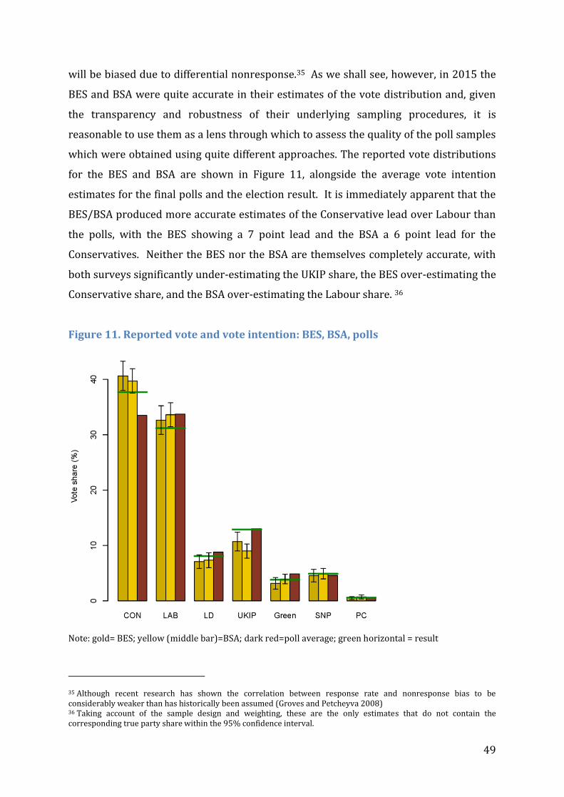
49
will be biased due to differential nonresponse.35 As we shall see, however, in 2015 the
BES and BSA were quite accurate in their estimates of the vote distribution and, given
the transparency and robustness of their underlying sampling procedures, it is
reasonable to use them as a lens through which to assess the quality of the poll samples
which were obtained using quite different approaches. The reported vote distributions
for the BES and BSA are shown in Figure 11, alongside the average vote intention
estimates for the final polls and the election result. It is immediately apparent that the
BES/BSA produced more accurate estimates of the Conservative lead over Labour than
the polls, with the BES showing a 7 point lead and the BSA a 6 point lead for the
Conservatives. Neither the BES nor the BSA are themselves completely accurate, with
both surveys significantly under-estimating the UKIP share, the BES over-estimating the
Conservative share, and the BSA over-estimating the Labour share. 36
Figure 11. Reported vote and vote intention: BES, BSA, polls
Note: gold= BES; yellow (middle bar)=BSA; dark red=poll average; green horizontal = result
35 Although recent research has shown the correlation between response rate and nonresponse bias to be considerably weaker than has historically been assumed (Groves and Petcheyva 2008) 36 Taking account of the sample design and weighting, these are the only estimates that do not contain the corresponding true party share within the 95% confidence interval.

50
On its own, this comparison is strongly suggestive that the polls underestimated the
Conservative lead as a result of their sampling procedures. However, it is ultimately
inconclusive because the BES/BSA differ from the polls in other respects, beyond their
sample designs. Most importantly, the BES/BSA were undertaken after the election had
taken place. This means that there was no uncertainty (at least by self-report) about
whether the respondents had voted or not when they reported their vote choice, while
the polls had to factor in whether a respondent would actually vote or not to their pre-
election estimates. The reported votes of the BES/BSA respondents might also have
been influenced by their knowledge of the election result, which could not have been
the case for the pre-election polls. Previous research has shown a tendency for
respondents to disproportionately recall having voted for the winning party – so called
‘bandwagoning’ (Nadeau, et al. 1993) and such effects might plausibly have contributed
to the difference in the lead estimates between the surveys and the polls in 2015.
Another potentially consequential difference between the BES/BSA and the polls is the
mode of interview, with the BES/BSA using face-to-face interviews and the polls using
either telephone interviews or online self-completion. There is, however, no obvious
reason to assume that face-to-face interviewing would, on its own, produce more
accurate self-reports of vote choice than the other modes. Indeed, the survey
methodological literature suggests that the face-to-face interviewing should be more
prone to measurement error due to socially desirable responding than other modes
(Tourangeau, et al. 2000). Nonetheless, these factors all render the headline
comparison between the polls and BES/BSA ambiguous with regard to the underlying
cause of the difference.
Fortunately, we can effectively rule out the two most important of these design
differences by considering the reported vote distributions for the polls that undertook
re-contact surveys. Because the re-contact surveys were carried out after the election,
we can exclude timing relative to the election as a potential confound.37 Figure 8 (page
37 A caveat to this conclusion is that the fieldwork periods were much shorter for the re-contact polls than for BES/BSA so ‘bandwagoning’ may have been more prevalent in the latter than the former case, although Mellon and Prosser (2015) demonstrate that this possibility has little empirical support, for the BES at least.
51
36) shows that the poll estimates38 of the Conservative lead do not noticeably improve
when the polls are undertaken after the election and respondents are reporting on their
actual, rather than their intended vote. These comparisons, then, support the
conclusion that the differences between the BES/BSA and the polls were due to
differences in their sampling procedures, rather than to whether they were undertaken
before or after the election.
In section 5 we noted that a key assumption in the methodology of opinion polls is that
the vote intention distribution is (approximately) correct within weighting cells. It is
informative, therefore, to assess the extent to which the polls differ from BES/BSA not
only in the aggregate but also across the weighting cells used by the pollsters. Figure
5.5 presents estimates of the Conservative/ Labour difference by age-band for the polls
and the BES/BSA (the BES/BSA estimates are combined due to small cell sizes within
age bands for each survey on its own).
Figure 12 shows that the estimates of the Conservative lead by age in the polls is
different to the BES/BSA estimates, particularly amongst those aged 45-64, where the
polls substantially under-estimate the Conservative lead. Here, of course, we must
assume that the BES/BSA distribution is correct within age-bands, although this does
not seem unreasonable, given that both surveys got the population estimate of the
Conservative lead approximately correct. Figure 13 plots the individual poll estimates
and the poll average on the lead against the election result at the Government Office
Region level39. Again, we see that the poll estimates of the Conservative lead within
regions are quite different to the election result. There is some indication in Figure 13
that the polls particularly under-estimated the Conservative lead in regions where the
Conservative vote share was higher than the national average.
38 These estimates are weighted to account for differential attrition between the pre-election poll and the re-contact survey. 39 Regional results are taken from (Hawkins, et al. 2015).
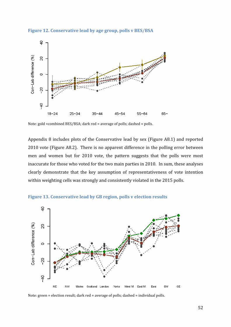
52
Figure 12. Conservative lead by age group, polls v BES/BSA
Note: gold =combined BES/BSA; dark red = average of polls; dashed = polls.
Appendix 8 includes plots of the Conservative lead by sex (Figure A8.1) and reported
2010 vote (Figure A8.2). There is no apparent difference in the polling error between
men and women but for 2010 vote, the pattern suggests that the polls were most
inaccurate for those who voted for the two main parties in 2010. In sum, these analyses
clearly demonstrate that the key assumption of representativeness of vote intention
within weighting cells was strongly and consistently violated in the 2015 polls.
Figure 13. Conservative lead by GB region, polls v election results
Note: green = election result; dark red = average of polls; dashed = individual polls.

53
A third type of comparison is informative about the representativeness of the poll
samples; an assessment of the accuracy of estimates for other variables that were
measured in the polls and which might themselves be related to vote choice. Consider,
for example, sector of employment; it is known that, broadly, public sector workers are
more likely to vote Labour and private sector workers are more likely to vote
Conservative (Dunleavy 1980). If polls that do not weight to population totals for
employment sector were found to have over-estimated the proportion of voters who
work in the public sector, then this would not only constitute evidence that the poll
samples were unrepresentative (with regard to employment sector), it would also
suggest a potential cause of the bias in the vote choice estimate. That is to say, by over-
representing public sector workers in their samples, the polls would have over-
estimated support for Labour and under-estimated support for the Conservatives.
This approach is particularly appealing because it indicates ways in which poll samples
might be improved in the future, either through changes to sample recruitment
procedures, or through improvements to quota and weighting targets (see for example
Mellon and Prosser 2015; Rivers and Wells 2015). Unfortunately, the extent to which
we are able to implement this strategy is constrained by the paucity of candidate
variables in the poll samples for which gold standard estimates are also available.
Variables which meet these twin criteria are, almost by definition, scarce. If they were
available, the pollsters would likely already be using them in their sampling and
weighting procedures. Nonetheless, some variables are available which enable us to
consider the polls from this perspective, albeit in a more limited manner than we would
ideally like.
Before presenting these analyses, an important caveat is in order. The logic of the
‘missing causal variable’ described above, is seductive. Once a diagnosis of
unrepresentative samples has been made, it is natural that the cause of the
unrepresentativeness should be sought and, ideally, corrected. However, the search for
the ‘missing’ variable is likely in our view to prove elusive. This is partly for the reason
noted above; if a variable possessing the required characteristics existed the pollsters
would likely already be using it. Additionally, it is unlikely that bias in the vote
intention estimate can be accounted for by a single direct cause. It is more plausible

54
that the underlying causal model linking survey participation to vote choice is a
complex multi-variable system, comprising interacting direct and indirect effects.
Another possible causal model is that bias in the vote intention estimate may not be
fully explained by any other measured or feasibly measurable variables, the case of
missing not at random (MNAR) in Rubin’s terminology (Rubin 1987). This latter case
would arise if vote intention were itself the direct cause of whether a voter responds to
a survey request or not. For example, nonresponse would be MNAR if Conservative
voters were more likely to decline a survey request because Conservatives consider
voting to be a private act that should not be shared with others.
To be clear, these are speculations, not hypotheses about what actually happened in
2015; the point of stating them here is to make clear that there are many potential
causes of unrepresentativeness in the poll samples and our ability to identify the
‘correct’ model is very limited. The examples that we present next should therefore be
seen as illustrations of evident sample bias in the polls, rather than as a complete
account of what went wrong in 2015.
The first example of biased poll estimates relates to the continuous age distribution
within banded age ranges. All pollsters weight their raw sample data to match the
distribution of banded ages in the population census. Three of the BPC members
(Opinium, TNS UK, and Yougov)40 also recorded continuous age, making it possible for
us to assess the age distribution within age bands and compare this to the distribution
from the census and the BES/BSA. Figure 14 shows this comparison for the oldest age
band, those aged 65 years and older. This shows that the polls substantially over-
represent people under the age of 70 and under-represent those aged 75 and older
within this age band, while the BES and BSA do not. Indeed, the three polls we are able
to consider here do not appear to contain a single respondent aged 90 or above.
40 These are all online pollsters so it is not clear form this analysis is the same effect is apparent in phone samples.

55
Figure 14. Continuous age distribution for 65+ age band (polls v census)
Note: green = census; gold = combined BES/BSA; dashed = individual polls
This is direct evidence that poll samples can produce quite biased estimates of
population characteristics. However, it also indicates the kinds of selection mechanism
which might, in part, have led to the 2015 polling miss. If the Conservative lead over
Labour was bigger amongst voters aged over 74 than those aged between 65 and 74
years, then under-representing the older age group would have biased the estimate of
the Conservative lead toward zero. In fact, the 2015 BES shows that the Conservatives
held a 21 point lead over Labour amongst those aged over 74 and a 22 point lead
amongst those aged 64-74. So the under-representation of voters aged 75 and over in
the poll samples seems unlikely to have made a notable contribution to the 2015 polling
miss 41.
Our second example also relates to the age distribution in the polls but this time we
consider the age of postal voters. Figure 15 shows the distribution of banded age for
postal voters in the polls (that asked whether respondents had voted by post) and in the
BES. If we take the BES as the gold-standard we can see that, although the polls get
some of the banded age distribution broadly correct, there is a tendency to over-
41 These within age-band estimates are based on samples of approximately 300, so have wide confidence intervals making it difficult to exclude the possibility that under-representation of those aged 75+ made a small contribution to the polling error.

56
represent the proportion in the 35-44 age group and to under-represent the proportion
of postal voters aged 65 and above. The BES also shows that Labour had a 9 point lead
over the Conservatives amongst those aged 35-44, while for those aged 65 and above,
the Conservatives led Labour by 22 points.
Figure 15. Banded age distribution for postal voters (polls v BES)
Note: gold = combined BES/BSA; dashed = polls
These errors in the age distribution of postal voters in the poll samples are therefore
likely to have contributed to the under-estimation of the Conservative lead over Labour.
However, because only 20.9% of ballots cast in 2015 were by post, the total
contribution of this error to the polling miss is likely to have been modest.
Our final example of biased estimates in the poll samples relates to over-estimation of
political engagement, an issue which has also been demonstrated by Rivers and Wells
(2015) and Mellon and Prosser (2015), albeit on YouGov data only. The only
consistently measured indicator of political engagement available across all nine BPC
pollsters is reported turnout in the 2010 General Election42. Figure 16 plots the self-
42 Turnout is a rather indirect measure of political engagement, though it is strongly associated with political interest. In the 2015 BES 69% of those who reported voting said they were either very or fairly interested in politics, the corresponding figure for those who did not vote was 31%.

57
reported 2010 turnout by age band, for the 2015 polls, the BES 43. Barring one notable
exception, the polls consistently over-estimate turnout in the 2010 election, although
the bias is particularly high amongst those aged 18-24.
Figure 16. Self-reported 2010 turnout by age band (polls v BES)
Note: gold= combined BES; dashed = individual polls
We noted in section 3 that SurveyMonkey was the only pollster to publish a poll in the
final week of the campaign with the correct estimate of the Conservative lead.
SurveyMonkey also used a rather different procedure from the other online pollsters to
recruit its sample (see section 5.1). It is therefore worth briefly considering whether
the SurveyMonkey result may have been due its approach to sample recrutiment
yielding a more representative sample than the other pollsters.
The first thing to note in this respect is that, despite getting the correct estimate of the
Conservative lead, the SurveyMonkey poll was substantially off on the individual party
shares, under-estimating the Conservatives by 4%, Labour by 3% and over-estimating
the Greens by 4%. Additionally, considering other variables collected as part of the
same poll, we can see that the SurveyMonkey sample over-represented the better
educated and the politically engaged in the same direction as the other polls. For
43 For the polls, these estimates use all the components of the estimation weights, except for predicted turnout probability, in other words, these estimates include the party identification component of the weights.
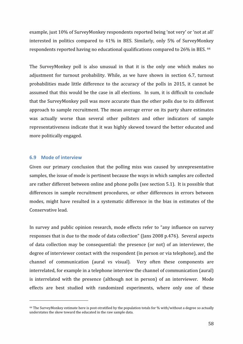
58
example, just 10% of SurveyMonkey respondents reported being ‘not very’ or ‘not at all’
interested in politics compared to 41% in BES. Similarly, only 5% of SurveyMonkey
respondents reported having no educational qualifications compared to 26% in BES. 44
The SurveyMonkey poll is also unusual in that it is the only one which makes no
adjustment for turnout probability. While, as we have shown in section 6.7, turnout
probabilities made little difference to the accuracy of the polls in 2015, it cannot be
assumed that this would be the case in all elections. In sum, it is difficult to conclude
that the SurveyMonkey poll was more accurate than the other polls due to its different
approach to sample recruitment. The mean average error on its party share estimates
was actually worse than several other pollsters and other indicators of sample
representativeness indicate that it was highly skewed toward the better educated and
more politically engaged.
6.9 Mode of interview
Given our primary conclusion that the polling miss was caused by unrepresentative
samples, the issue of mode is pertinent because the ways in which samples are collected
are rather different between online and phone polls (see section 5.1). It is possible that
differences in sample recruitment procedures, or other differences in errors between
modes, might have resulted in a systematic difference in the bias in estimates of the
Conservative lead.
In survey and public opinion research, mode effects refer to “any influence on survey
responses that is due to the mode of data collection” (Jans 2008 p.476). Several aspects
of data collection may be consequential: the presence (or not) of an interviewer, the
degree of interviewer contact with the respondent (in person or via telephone), and the
channel of communication (aural vs visual). Very often these components are
interrelated, for example in a telephone interview the channel of communication (aural)
is interrelated with the presence (although not in person) of an interviewer. Mode
effects are best studied with randomized experiments, where only one of these
44 The SurveyMonkey estimate here is post-stratified by the population totals for % with/without a degree so actually understates the skew toward the educated in the raw sample data.
59
components is varied and the others are held constant. Observational studies, such as
we are using here, cannot satisfactorily differentiate measurement effects of mode from
those caused by differences in coverage, sampling, and nonresponse, to name but the
most important sources of polling error. In interpreting our comparisons between the
results of telephone and online polls, then, it must be borne in mind that observed
differences combine multiple sources of error.
Considering the final poll estimates (see Table 1 section 3), there is no difference in
accuracy between online and telephone polls. The average estimate of the Conservative
lead over Labour was -0.2% for phone and online polls and the mean average error in
the vote shares of the seven largest parties was 1.6% for both modes. However, it is
important to consider mode differences over a more extended period, not least because
the expectation of a dead heat in the election and the effect this had in terms of framing
debate had formed long before the final week of the short campaign.
Figure 17 shows the poll estimates of the Con-Lab margin between 2010 and 2015 by
mode. 45 The difference in estimates of the Conservative lead between phone and online
polls is shown in Figure 18 (positive scores indicate a larger Conservative lead for
phone compared to online). Immediately after the 2010 election, online polls showed
somewhat higher support for the Conservatives, by a margin of around 1%. This
reversed at the beginning of 2011 and, from then until 2014 phone polls tended to show
higher support for the Conservatives, with differences varying between 1% and 2.5%.
This mode difference then disappeared for most of 2014, re-emerging in early 2015 and
increasing as the election approached, including during the short campaign. Phone
polls during the short campaign averaged a small Conservative lead, in the order of 2%,
while online polls during the same period showed a Labour lead of slightly less than 1%.
As already noted, this mode difference disappeared completely at the end of the short
campaign.
45 These moving averages are estimated using a random-walk model, assuming correlated movements between online and phone polls, and weighting polls by their sample size.

60
Figure 17. Conservative lead 2010-2015 by interview mode of polls
Of course, the true distribution of vote choice is known only on Election Day, so it is
difficult to interpret a mode difference weeks or months before an election as indicating
that one mode is more accurate than another. That said, we cannot ignore the fact that
the 2015 polls substantially under-estimated the Conservative lead over Labour, a
pattern which has been evident for the past thirty years. In this context, it is not
unreasonable to assume that the generally higher Conservative share in the phone polls
indicates that they were somewhat more accurate during the campaign period but this
is, to be clear, only an assumption.
That this difference disappeared at the end of the may be related to herding (see section
7) but it may also be because there is no strong reason to expect these kinds of mode
differences to be stable over time. This is because mode effects arise from the
interaction of the political environment with the various errors to which polling
methods are prone. The magnitude and direction of these mode effects in the middle of
the election cycle may be quite different to those that are evident in the final days of the
campaign.
2011 2012 2013 2014 2015 2016
−10
−5
05
10
Con−Lab Margin by Mode of Data Collection
Date
Con−
Lab M
arg
in
Online
Telephone
● Result
●●Final
Polls
2011 2012 2013 2014 2015 2016
−4
−2
02
4
Mode of Data Collection Difference
Date
Ph
one −
Onlin
e (
Con−
Lab M
arg
in)
●Final
Polls

61
Figure 18. Mode Difference in Conservative lead, polls 2010-2015
2011 2012 2013 2014 2015 2016
−1
0−
50
51
0
Con−Lab Margin by Mode of Data Collection
Date
Co
n−
La
b M
arg
in
Online
Telephone
● Result
●●Final
Polls
2011 2012 2013 2014 2015 2016
−4
−2
02
4Mode of Data Collection Difference
Date
Ph
on
e −
On
line (
Co
n−
La
b M
arg
in)
●Final
Polls

62
7. Herding
It was not simply that the polls got the outcome of the election wrong but the unanimity
with which they came to the conclusion of a dead heat that led to the collective shock
when the result was known. In this section we consider whether the convergence in the
estimates of the lead in the final weeks of the campaign might have been due to
‘herding’. The American Association for Public Opinion Research (AAPOR) defines
herding in the following way:
“Herding” specifically refers to the possibility that pollsters use existing poll
results to help adjust the presentation of their own poll results. "Herding”
strategies can range from making statistical adjustments to ensure that the
released results appear similar to existing polls to deciding whether or not to
release the poll depending on how the results compare to existing polls.”46
The AAPOR definition implies a conscious taking of cues from other pollsters. However,
pollsters may take these cues unconsciously, or may engage in behaviours that reduce
polling variance without taking any cues from other pollsters at all.47 It is important to
be clear, then, that while we will retain the word “herding” for consistency with existing
use, this does not imply that we believe that pollsters deliberately made choices that
pushed their results towards consensus, though we cannot rule this possibility out
either.
There are several ways in which pollsters could make choices that have the effect of
reducing the variation in their results. These include, but are not limited to:
1) adapting post-stratification and turnout weighting procedures in order to make
estimates conform with expectations of the likely result
2) expanding the sample size for a poll when the initial results do not agree with
expectations of the likely result
46 American Association for Public Opinion Research “Herding” http://www.aapor.org/AAPORKentico/Education-Resources/Election-Polling-Resources/Herding.aspx 47 For example, by suppressing polls that are out of line with their own past polling, regardless of what other pollsters are reporting
63
3) suppressing (not publicly reporting) polls that do not agree with expectations
of the likely result
All of these are related to pollsters’ expectations, and so we note that there are three
distinct expectations towards which pollsters might plausibly converge at the end of the
campaign period. First, they might converge towards their own past polling results,
based on recognition that some of the change from poll to poll is likely to be sampling
variability. Second, the pollsters might converge towards the collective average of
recently published polls. Herding towards the average of recent polls would be
appealing for a pollster wishing to accurately match the election results, or at least be
no more wrong than the other pollsters. Just as it is reasonable for poll aggregators to
pool the information across all public polls, a pollster forming expectations about the
result would naturally look to what other pollsters are reporting. Third, the pollsters
might converge towards a tied election between the main parties; this would reduce the
risk of a “wrong prediction” of the leading party.
The first two types of herding, towards the polling average, cannot alone explain the
systematic bias of the polls in 2015. If polls were unbiased, they would have herded
towards unbiased results. If the polls were biased for other reasons, a finding of
herding towards the polling average would help explain why all pollsters ended up on
the same wrong answer. In contrast, herding towards neutrality on the Conservative-
Labour margin could alone explain both the systematic miss of the pollsters and the
similarity of the reported margins.
Analyses of polls in the US have shown evidence of herding (Clinton and Rogers 2013;
Linzer 2012; Silver 2014). In the UK Singh (2015b) found no evidence of herding in the
2015 election. However, he used the theoretical variance of a simple random sample
(SRS) of a fixed size as the baseline expectation for variability. We do not rely on this
assumption because the true sampling variability of the procedures that pollsters
actually use – which is not observed - is likely to be different from SRS. While weighting
generally increases the variance of estimates, stratification has the opposite effect, if the
stratification variables are correlated with vote intention. This is likely to be the case for

64
the polls because they use past vote or party identification for post-stratification, which
could substantially reduce the sampling variability of the methods employed.
Most pollsters increased their sample sizes in their final polls, so, under almost any
sampling design, we would expect the sampling variance to decline. The question we
must ask is whether the variation in the vote shares declined by more than we would
expect, given the larger sample sizes. We will assume for the purposes of the following
analysis that the rate at which variation decreases as sample size increases is
proportionate to what would be observed under SRS, but not that the baseline level of
sampling variability is equal to SRS. A description of the statistical procedures used and
the assumptions on which they are based is provided in Appendix 6.
In the final week before the election, there is a strong downward trend in the observed
variance of the Conservative-Labour margin, relative to what we would expect given the
sample sizes of the polls.48 While the downward trend is visually suggestive, we cannot
reject the null hypothesis of zero change. 49 However, a lack of statistical significance in
the time trend does not mean there was no time trend, in fact it is probably more
indicative of the small number of observations on which the test is based. The decline
in the estimated variance across pollsters is substantial in absolute magnitude,
dropping by half between the early campaign and the day before the election.
48 For individual parties (not shown), the trends are more varied and there is no clear evidence of downward trends in the final period of the campaign. 49 using an F-test of the spline regression (p=0.27)

65
Figure 19. Assumed & observed variance in poll estimates, Conservative lead
If herding arose through pollsters making methodological changes over time, a
precondition for herding to have taken place is that methodological changes were
actually implemented. And, indeed, five of the BPC pollsters changed their methods
during the short campaign. Did these particular methodological changes lead to
convergence in the estimates on the lead? To assess this, we take the raw data for the
final campaign polls for each pollster, and re-estimate the Conservative-Labour margin
using the procedures employed in the first campaign polls. We compare the variation in
the published final polls to the variation that would have been observed if the
methodology had remained constant same throughout the period. The results of this
analysis are presented in Figure 20. This shows that the weighting procedures used by
the pollsters in their final polls did tend to shift the reported Conservative-Labour
margin in the correct direction, that is toward a larger lead for the Conservatives. The
modified procedures also reduced the variation in the estimates, though not by very
much. On the variance scale used in the analysis of the pollster variability, using the
early campaign weightings increases the scaled deviations by less than 10% in the final
polls, versus the doubling that would be necessary to bring the variance up to the level
of the early campaign polls. Therefore, these specific changes in adjustment procedures
used by the pollsters account for only a small fraction of the decrease in variability in
the poll estimates over the course of the campaign.
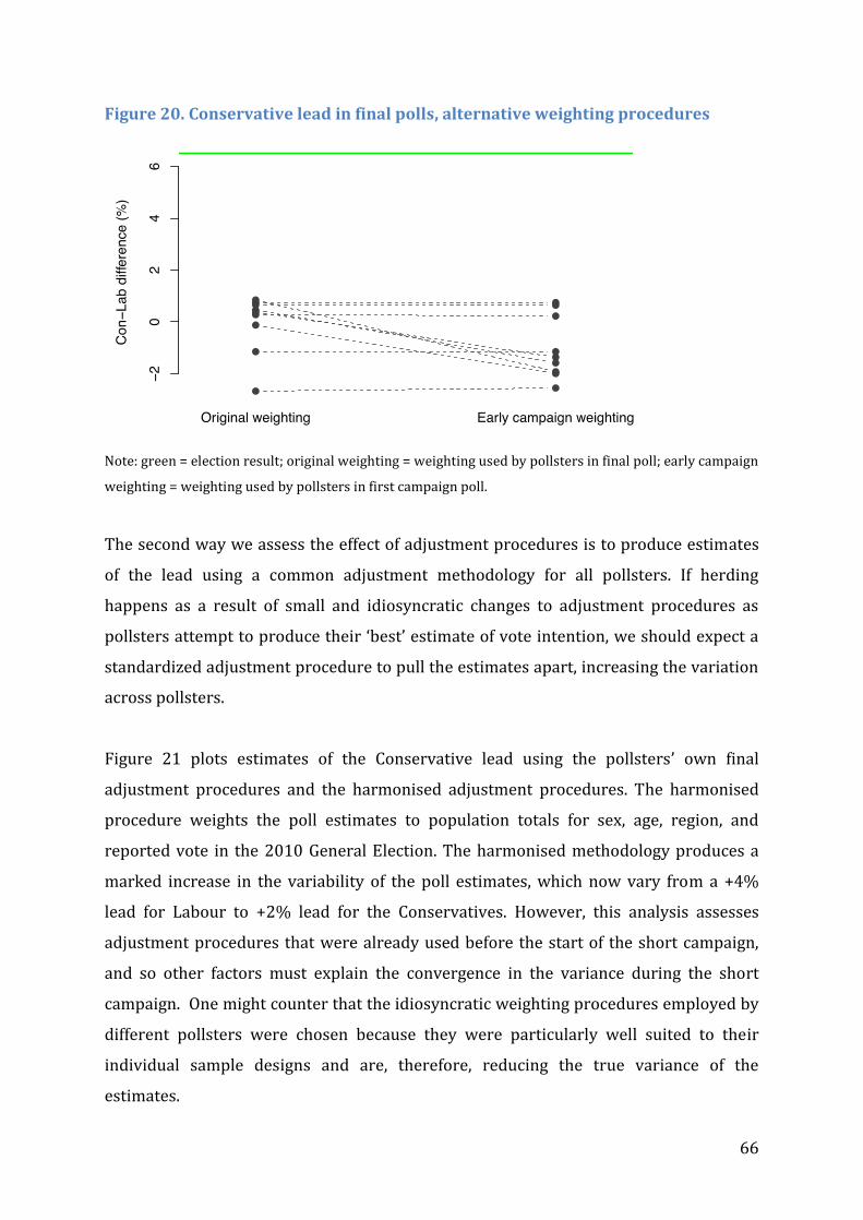
66
Figure 20. Conservative lead in final polls, alternative weighting procedures
Note: green = election result; original weighting = weighting used by pollsters in final poll; early campaign
weighting = weighting used by pollsters in first campaign poll.
The second way we assess the effect of adjustment procedures is to produce estimates
of the lead using a common adjustment methodology for all pollsters. If herding
happens as a result of small and idiosyncratic changes to adjustment procedures as
pollsters attempt to produce their ‘best’ estimate of vote intention, we should expect a
standardized adjustment procedure to pull the estimates apart, increasing the variation
across pollsters.
Figure 21 plots estimates of the Conservative lead using the pollsters’ own final
adjustment procedures and the harmonised adjustment procedures. The harmonised
procedure weights the poll estimates to population totals for sex, age, region, and
reported vote in the 2010 General Election. The harmonised methodology produces a
marked increase in the variability of the poll estimates, which now vary from a +4%
lead for Labour to +2% lead for the Conservatives. However, this analysis assesses
adjustment procedures that were already used before the start of the short campaign,
and so other factors must explain the convergence in the variance during the short
campaign. One might counter that the idiosyncratic weighting procedures employed by
different pollsters were chosen because they were particularly well suited to their
individual sample designs and are, therefore, reducing the true variance of the
estimates.

67
We found no evidence of convergence with respect to the individual party shares and
this might be viewed as evidence against herding. However, it is possible for the
pollsters to herd on the lead, but not on the levels of the party shares. Consider one
hypothetical mechanism by which herding might have occurred. If pollsters were
adjusting their weighting schemes they would have known that most other pollsters
were reporting Conservative-Labour leads of close to zero. If they observed that some
weighting adjustments produced large leads in either direction, they may have been less
inclined to choose those weightings, compared to others which did not have such a large
effect on the lead. However, if a pollster considered a weighting change that yielded a
35-35 poll, rather than a 33-33, it would make no difference to the lead. The
Conservative-Labour lead is the headline figure when pre-election polls are presented,
the absolute levels (despite their consequence for comparison with all other parties)
receive far less attention. This is particularly true because the level of the vote for
minor parties is difficult to predict and inconsequential for government formation.
Thus, herding could occur with respect to the lead without occurring with respect to
those or other parties’ levels.
Figure 21. Conservative lead: actual v harmonised adjustment procedures
Note: green = election result; original weighting = weighting used by pollsters in final poll; harmonised
weighting = weighting using harmonised weight.

68
In summary, we have shown that a) variation in the poll estimates of the Conservative
lead was considerably lower than would be expected given liberal assumptions about
the true variance b) pollsters changed their adjustment procedures during the short
campaign c) the changed procedures resulted in a small reduction in the variation of the
Conservative lead and d) using a harmonised adjustment procedure for the final
estimates across all pollsters results in a substantial increase in the variation of the
Conservative lead. Taken together, this evidence leads us to conclude that herding may
have contributed to the surprisingly high consensus between pollsters in the final polls
of the 2015 general election.

69
8. Conclusions and recommendations
In the months and weeks leading up to the 2015 general election the polls told a
consistent story; the Conservatives and Labour were in a dead heat in the popular vote.
This led media commentators, party strategists, and the public to focus attention on the
likely composition of a coalition, rather than on a single-party government led by the
Conservatives who, of course, ultimately won the election with a 6.6% lead over Labour
and an absolute majority in the House of Commons. The expectation of a hung
parliament in the final days and weeks of the campaign was so strong and widely held
that the sense of shock and disbelief was palpable when the result of the exit poll was
announced at 10pm on May 7th.
Questions were soon being asked about the role of the polls in creating a false collective
expectation about the likely outcome of the election and media sponsors publicly
questioned the quality and value of the polling they had commissioned. At least one
national newspaper stated that it would afford less prominence to opinion polling in its
political coverage in the future. Politicians and peers suggested that the polling
inaccuracies had affected the outcome of the election, speculating that Labour might
have done better had the polls been accurate. A private members’ bill was introduced
in the House of Lords on 28th May, proposing state regulation of the polling industry50.
Concern was also expressed by social and market research industry professionals. As
the most direct way the public encounters survey and opinion research, it was feared
that the failure of the polls might have negative consequences for public confidence in
social and market research and official statistics more generally.
In this report to the British Polling Council and the Market Research Society we have
considered a broad range of evidence in order to assess what caused the polls –
collectively and individually – to produce inaccurate estimates of the national vote
shares in 2015. Our conclusion is that the primary cause of the polling miss was
unrepresentative samples. The methods the pollsters used to collect samples of voters
systematically over-represented Labour supporters and under-represented
50 Regulation of Political Opinion Polling Bill [HL] 2015-16.
70
Conservative supporters. The statistical adjustment procedures applied to the raw data
did not mitigate this basic problem to any notable degree.
We came to this conclusion partly by elimination of other putative causes of the error.
First, we were able to replicate all published estimates for the first, the penultimate, and
the final polls using the raw micro-data provided by the BPC pollsters. This enabled us
to rule out the possibility that at least some of the errors might have been caused by
flawed analysis, or by use of inaccurate weighting targets on the part of the pollsters.
We were also able to exclude the possibility that postal voters, overseas voters, and un-
registered voters made any detectable contribution to the polling errors. The ways that
pollsters asked respondents about their voting intentions was also eliminated as a
possible cause of what went wrong.
We found weak evidence that there may have been a very modest late swing to the
Conservatives between the final polls and Election Day, although this can have
contributed – at most – around one percentage point to the mean absolute error on the
Conservative lead. The widely held view that the polling miss was due to deliberate
misreporting - ‘shy Tories’ telling pollsters they intended to vote for other parties - is
difficult to reconcile with the results of the re-contact surveys carried out by the
pollsters and with the two random surveys undertaken after the election. We reject
deliberate misreporting as a contributory factor in the polling miss. Differential turnout
was also pointed to after the election as a likely cause of the errors; so-called ‘lazy
Labour’ supporters telling pollsters they would vote Labour but ultimately not turning
out to vote. Data from a number of sources shows no support for differential turnout
misreporting making anything but a very small contribution to the polling errors.
That these factors did not contribute, in anything other than a trivial way, to the polling
miss in 2015 does not mean that they might not cause more substantial problems in the
future. Current practice can be improved in several respects. We recommend that BPC
members should:

71
1. include questions during the short campaign to determine whether respondents
have already voted by post. Where respondents have already voted by post they
should not be asked the likelihood to vote question.
2. review existing methods for determining turnout probabilities. Too much
reliance is currently placed on self-report questions which require respondents
to rate how likely they are to vote, with no clear rationale for allocating a turnout
probability to the answer choices.
3. review current allocation methods for respondents who say they don’t know, or
refuse to disclose which party they intend to vote for. Existing procedures are ad
hoc and lack a coherent theoretical rationale. Model-based imputation
procedures merit consideration as an alternative to current approaches.
If all the potential causes considered above are ruled out, we are left to conclude that
unrepresentativeness in the samples must have been the cause of the polling miss in
2015. On its own, a strategy which reaches a conclusion through elimination of
alternative explanations is not very satisfactory, particularly when the evidence on
which the preliminary eliminations are based is imperfect, as is the case here. Had we
been drawn, by a process of elimination, to conclude that the polling miss was due to a
prima facie implausible explanatory factor - such as overseas voters - then we would
question the validity of the process that led us to this inference. But this is not the case
here; we have identified sampling and weighting procedures as representing inherent
weaknesses of polling methodology (see section 5). It is also worth noting, in this
context, that the report into the 1992 UK election polls and the AAPOR report into the
2008 US Presidential primary polls both concluded that unrepresentative samples were
contributory factors in those errors, so there is also a historical precedent for this
conclusion.51
What can be done to improve the representativeness of poll samples in the future? The
answer to this question depends on whether the pollsters continue to employ quota
methods, or switch to random sampling. Due to the high cost of random sampling, we
expect the vast majority of opinion polls to continue using non-random sampling
51 The 1992 report does not refer directly to unrepresentative samples but to inaccurate quota controls, the basic conclusion however is the same.

72
methods for the foreseeable future. However, continuing with non-random sampling
means there are only two broad strategies that can be pursued to improve sample
representativeness. Pollsters can take measures to increase the representativeness of
respondents recruited to existing quota and weighting cells, or they can incorporate
new variables into their quota and weighting schemes which are more related to both
the probability of selecting into poll samples and vote intention. These are not mutually
exclusive strategies, both can be pursued. We therefore recommend that:
4. Pollsters should take measures to obtain more representative samples within
the weighting cells they employ.
How this is done will depend, to an extent, on the mode of the poll. For phone polls this
is likely to involve (but will not be limited to) using longer fieldwork periods, more call-
backs to initially non-responding numbers (both non-contacts and refusals), and
ensuring a better mix52 of landline and mobile phone numbers. We understand that,
taken to their logical extreme, these procedures would be practically equivalent to
implementing a random probability design and would therefore be expensive and time-
consuming. While, as we will note shortly, we would very much welcome the
implementation of truly random sample designs, we acknowledge that the cost
restrictions of true random methods make them impractical for the vast majority of
phone polls. Nevertheless, it would seem that there are gains to be made in quality
without making the resultant design un-affordably expensive and lengthy. It may be
that implementing procedures of this nature results in fewer polls being carried out
than was the case in the last parliament, as the cost of undertaking each one would no
doubt increase. This would, in our view be no bad thing, so long as the cost savings that
accrue from doing fewer polls are invested in quality improvements.
For online polls the procedures required to yield more representative samples within
weighting cells are also likely to involve longer field periods, more reminders, as well as
differential incentives for under-represented groups, and changes to the framing of
survey requests. We encourage online pollsters to experiment with these and other
52 Better in the sense of reflecting the population distribution of landline, mobile and dual-phone use.
73
methods in order to increase the diversity of their respondent pools. It is worth noting
in this context, that the only online pollster to get the correct mix of Conservative and
Labour supporters in their sample (albeit at the wrong absolute levels) was
SurveyMonkey. The procedure employed by SurveyMonkey to recruit respondents is
rather different to other online pollsters and might be capable of reaching a larger and
more diverse pool of potential respondents but this is no more than speculation at this
point in time. The performance of SurveyMonkey must be considered in the context of
its higher mean absolute error on the party vote shares compared to the average of the
other pollsters.
The second strategy pollsters can pursue to improve sample representativeness is to
modify the variables used to create quota and weighting cells. We therefore recommend
that:
5. Pollsters should investigate new quota and weighting variables which are
correlated with propensity to be observed in the poll sample and vote intention.
In our judgement the first of these strategies (recommendation 4) is likely to prove
more fruitful than the second (recommendation 5). This is because it is likely that, if
variables that are correlated with self-selecting into opinion polls and vote intention
were readily available, pollsters would already be using them. In making
recommendation 5, we add a note of caution regarding the use of variables which do not
have well defined and reliably known population totals. This is because the use of such
variables might do more harm than good to the accuracy of estimates and may also
serve as a facilitator of herding behaviour.
It is worth noting at this point that, while there was no difference in the error of the
final poll estimates between modes of interview, there was a small but systematic
tendency for the phone polls to yield somewhat higher estimates of the Conservative
vote share throughout most (but not all) of the 2010-2015 parliament, including for
much of the short campaign. It is not possible to say what the cause of this difference
was from the data that was available to us. However, it would not be unreasonable to
think that it might be related to the different approaches to sampling of phone and
74
online polls. It is likely that the propensity to be contacted and to agree to an interview
request by a phone pollster is somewhat different to that for selecting into an online
panel and that these differential propensities might be correlated with vote intention.
We encourage the polling industry to undertake further research into the underlying
cause(s) of these variable mode differences.
While we wish to be clear that we are not recommending that pollsters should switch en
masse to random sampling, this is only because we recognise the cost of doing so would
be prohibitive. Given recent developments in random online survey capabilities53, we
regard the timeliness argument against random sampling to be no longer as relevant as
it was in the past. If a way can be found, either individually or collectively, for poll
sponsors to fund a random probability design during the short campaign, this would
unquestionably be a positive development. There is, of course, no guarantee that a
random probability survey would get the vote intention estimate correct. But it would
reduce the risk of being wrong and, moreover, would represent a very useful means for
non-random polls to benchmark their estimates, not only in terms of the headline vote
intention but also to a range of other measured variables, some of which might be used
in setting quota and weighting targets. We recognise that it is unlikely that a private
funder or funders will underwrite the costs of a random probability design for a pre-
election opinion poll. Given the high public, commercial, and political interest in the
pre-election poll estimates, we therefore recommend that:
6. The Economic and Social Research Council (ESRC) should fund a pre as well as
a post-election random probability survey as part of the British Election Study
in the 2020 election campaign.
An exciting possibility for the implementation of a pre-election random probability
sample would be for it to be administered as part of a randomly recruited online panel.
These are now common in many comparator nations but the UK is yet to implement
one.
53 It is now feasible for samples to be collected using random probability methods and for respondents to complete questionnaires online using smartphones and tablets as a panel (see Callegaro, et al. 2014). Surveys using this kind of approach could produce estimates of vote intention during an election campaign in not much more time than is currently required for a telephone poll.
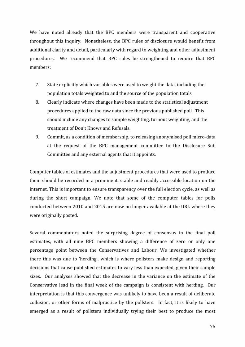
75
We have noted already that the BPC members were transparent and cooperative
throughout this inquiry. Nonetheless, the BPC rules of disclosure would benefit from
additional clarity and detail, particularly with regard to weighting and other adjustment
procedures. We recommend that BPC rules be strengthened to require that BPC
members:
7. State explicitly which variables were used to weight the data, including the
population totals weighted to and the source of the population totals.
8. Clearly indicate where changes have been made to the statistical adjustment
procedures applied to the raw data since the previous published poll. This
should include any changes to sample weighting, turnout weighting, and the
treatment of Don’t Knows and Refusals.
9. Commit, as a condition of membership, to releasing anonymised poll micro-data
at the request of the BPC management committee to the Disclosure Sub
Committee and any external agents that it appoints.
Computer tables of estimates and the adjustment procedures that were used to produce
them should be recorded in a prominent, stable and readily accessible location on the
internet. This is important to ensure transparency over the full election cycle, as well as
during the short campaign. We note that some of the computer tables for polls
conducted between 2010 and 2015 are now no longer available at the URL where they
were originally posted.
Several commentators noted the surprising degree of consensus in the final poll
estimates, with all nine BPC members showing a difference of zero or only one
percentage point between the Conservatives and Labour. We investigated whether
there this was due to ‘herding’, which is where pollsters make design and reporting
decisions that cause published estimates to vary less than expected, given their sample
sizes. Our analyses showed that the decrease in the variance on the estimate of the
Conservative lead in the final week of the campaign is consistent with herding. Our
interpretation is that this convergence was unlikely to have been a result of deliberate
collusion, or other forms of malpractice by the pollsters. In fact, it is likely to have
emerged as a result of pollsters individually trying their best to produce the most

76
accurate estimate through implementation of (idiosyncratic) adjustment procedures.
Ultimately, however, we are not able to determine the exact cause of the convergence in
estimates during the final days of the campaign. Convergence in poll estimates can
occur for reasons entirely unconnected with the behaviour of the pollsters. To make it
easier to rule out herding as a cause of convergence at future elections, we recommend
that BPC rules should require members to:
10. pre-register vote intention polls with the BPC prior to the commencement of
fieldwork. This should include basic information about the survey design such
as mode of interview, intended sample size, quota and weighting targets, and
fieldwork dates.
Pre-registration of vote intention polls does not mean herding cannot happen in the
future. However, it would provide a record that could subsequently demonstrate that
poll suppression, applying stopping rules on sample size, and arbitrary changes to
adjustment procedures had not occurred.
The inquiry was also tasked with assessing whether uncertainty in poll estimates is
adequately communicated to stakeholders and the public. Our conclusion is that it is
not. Media commentators generally use a rule of thumb that point estimates of party
shares have a margin of error of + or - three percentage points. This is (or appears to
be) based on the calculation of a 95% confidence interval for a simple random sample of
1000 respondents for a party with 50% of the vote. But polls are not simple random
samples, parties are typically far from 50% of the vote, and when the full sample is 1000
the number of respondents used for estimating party shares is much less than this
number. For these reasons, the true margin of error will usually be different from + or –
3 per cent, sometimes larger and sometimes smaller, depending on the specifics of the
research design. Pollsters should therefore aid the interpretation of their findings by
providing media clients with confidence intervals that better reflect the research design
than is currently the case.
The confidence intervals and information about how they were calculated should be
published with the computer tables required by the BPC rules. BPC members should
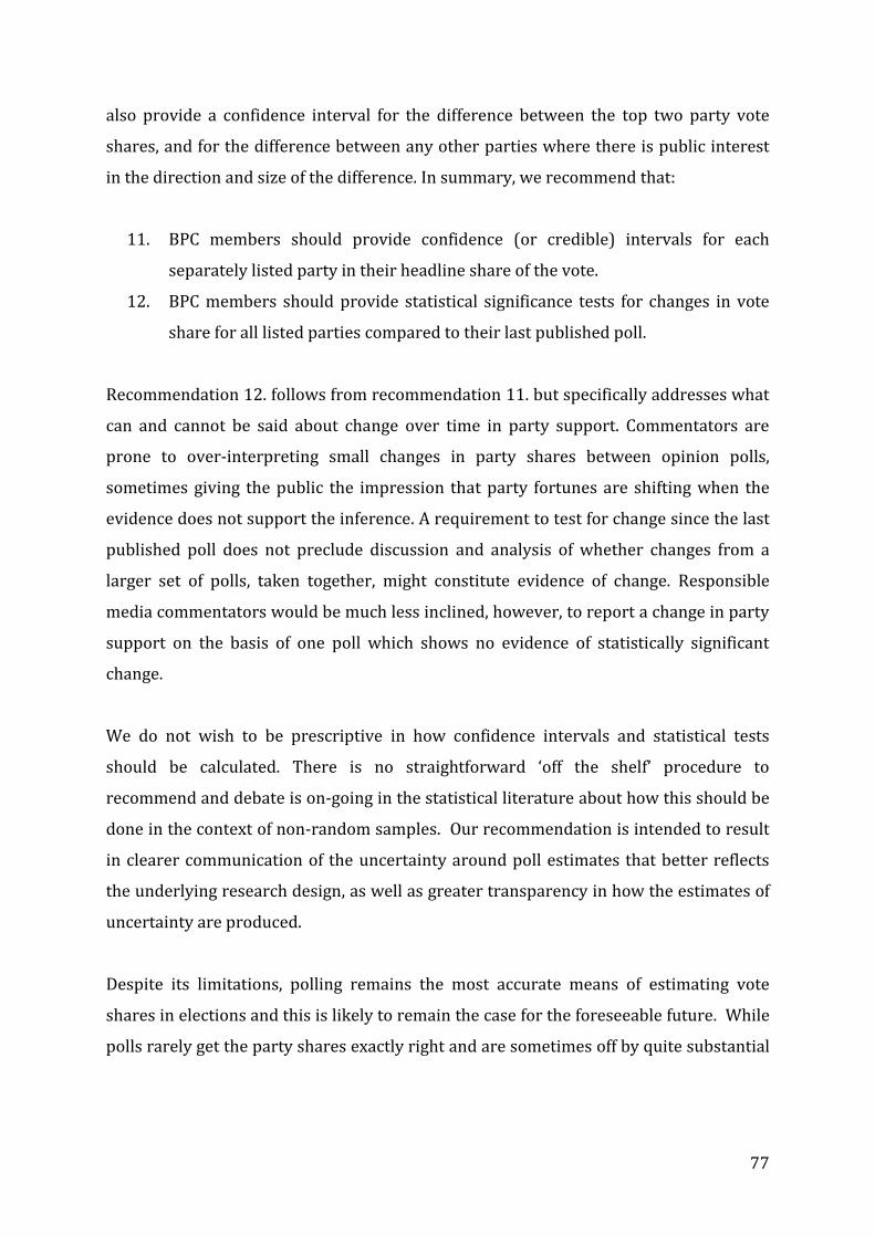
77
also provide a confidence interval for the difference between the top two party vote
shares, and for the difference between any other parties where there is public interest
in the direction and size of the difference. In summary, we recommend that:
11. BPC members should provide confidence (or credible) intervals for each
separately listed party in their headline share of the vote.
12. BPC members should provide statistical significance tests for changes in vote
share for all listed parties compared to their last published poll.
Recommendation 12. follows from recommendation 11. but specifically addresses what
can and cannot be said about change over time in party support. Commentators are
prone to over-interpreting small changes in party shares between opinion polls,
sometimes giving the public the impression that party fortunes are shifting when the
evidence does not support the inference. A requirement to test for change since the last
published poll does not preclude discussion and analysis of whether changes from a
larger set of polls, taken together, might constitute evidence of change. Responsible
media commentators would be much less inclined, however, to report a change in party
support on the basis of one poll which shows no evidence of statistically significant
change.
We do not wish to be prescriptive in how confidence intervals and statistical tests
should be calculated. There is no straightforward ‘off the shelf’ procedure to
recommend and debate is on-going in the statistical literature about how this should be
done in the context of non-random samples. Our recommendation is intended to result
in clearer communication of the uncertainty around poll estimates that better reflects
the underlying research design, as well as greater transparency in how the estimates of
uncertainty are produced.
Despite its limitations, polling remains the most accurate means of estimating vote
shares in elections and this is likely to remain the case for the foreseeable future. While
polls rarely get the party shares exactly right and are sometimes off by quite substantial

78
margins, they are considerably more accurate than any of the existing alternatives.54
Yet, it must be better acknowledged that accurately predicting vote shares in an election
is a very challenging task. A representative sample of the general population must be
obtained and accurate reports of party choice elicited from respondents. An
approximately accurate method of determining how likely respondents are to cast a
vote must be implemented and the sample of voters must not change their minds
between taking part in the poll and casting their ballots. What is more, the entire
procedure must usually be carried out and reported on within a very short space of time
and at very low cost. Given these many potential pitfalls, it should not be terribly
surprising that the historical record shows polling errors of the approximate magnitude
of 2015 occur at not infrequent intervals.
Some of the recommendations we have set out in this report are likely, if implemented,
to result in a lower volume of polls being carried out in the future. We have already
remarked that it would be a positive development if a reduction in the quantity of polls
were mirrored by a corresponding improvement in quality. In survey and opinion
research, as in many areas of life, cost and quality are related, if not quite in lock-step.
Yet spending more on opinion polls will be no guarantee of accuracy. Indeed, a
desirable legacy for this report is that it might effect a more realistic appraisal amongst
stakeholders of the limits of sample based research to predict the future behaviour of
complex, dynamic, and reflexive populations.
It is worth reflecting, in this context, on the fact that the 2015 British Election Study
face-to-face survey was carried out over a period of several months after the election,
used the highest quality methods at all stages and came with a price tag that reflected
this. Yet it still managed to over-estimate the Conservative and under-estimate the
UKIP vote shares by statistically significant margins. This should tell us that there will
be no silver bullet for the problem of polling errors.
54 Some might contend that betting markets can be more accurate than the polls but this was not the case in 2015. It is also something of a circular argument, as the primary drivers of the odds on the party shares are the results of the opinion polls.

79
This is not a council of despair, however. There are improvements that can and should
be made to how polling is currently practised in the UK and the recommendations in
this report point to ways in which this can be done. Some of the changes we
recommend are tweaks and modifications to existing procedures, others are more
ambitious and look to harness emerging technologies to undertake polls in new and
innovative ways. Alongside these methodological changes must come greater
transparency about how polls are conducted and clearer communication of the likely
levels of uncertainty in their estimates.

80
9. References
AAPOR 2008 'Standard Definitions: Final Dispositions of Case Codes and Outcome Rates
for Surveys', Illinois: American Association for Public Opinion Research.
— 2009 'An Evaluation of the Methodology of the 2008 Pre-Election Primary Polls':
American Association for Public Opinion Research.
Butler, D. and Pinto-Duschinsky, M. 1971 The British General Election of 1971, London:
Macmillan.
Callegaro, M., Baker, R. P., Bethlehem, J., Goritz, A. S., Krosnick, J. A. and Lavrakas, P. J.
2014 Online Panel Research: A Data Quality Perspective: Wiley.
Clinton, J. and Rogers, S. 2013 'Robo-Polls: Taking Cues from Traditional Sources?', PS:
Political Science & Politics 46: 333-337.
Curtice, J. 2016 'The Benefits of Random Sampling Lessons from the 2015 UK General
Election', London: NatCen Social Research.
Curtice, J. and Firth, D. 2008 'Exit polling in a cold climate: the BBC-ITV experience in
Britain in 2005', Journal of the Royal Statistical Society - Series A: Statistics in Society
171(3): 509-539.
Curtice, J., Fisher, S. and Kuha, J. 2011 'Confounding the commentators: How the 2010
exit poll got it (more or less) right', Journal of Elections, Public Opinion & Parties(21):
211-235.
Dunleavy, P. 1980 'The Political Impliations of Sectoral Cleavages and the Growth of
State Employment: Part 1, The Analysis of Production Cleavages', Political Studies 28(3):
364-383.
Fisher, S. 2016 'Piecing it all together and forecasting who governs: The 2015 British
general election', Electoral Studies.
Ford, R., Will Jennings, Mark Pickup and Christopher Wlezien 2016 'From Polls to Votes
to Seats: Forecasting the 2015 British general election', Electoral Studies.
Groves, R. 1989 Survey errors and survey costs, New York: Wiley.
Hawkins, O., Keen, R. and Nakatudde, N. 2015 'General Election 2015'.
Hopkins, D. 2009 'No More Wilder Effect, Never a Whitman Effect: When and Why Polls
Mislead about Black and Female Candidates', The Journal of Politics 71(3): 769-781.
Jans, M. 2008 'Mode effects', in P. J. Lavrakas (ed) Encyclopedia of survey research
methods, Vol. 2, Thousands Oaks, CA: Sage: 475-80.
81
Jennings, W. and Wlezien, C. 2016 'The Timeline of Elections: A Comparative
Perspective', American Journal of Political Science 60(1): 219-233.
Jowell, R., Hedges, B., Lynn, P., Farrant, G. and Heath, A. 1993 'Review: The 1992 British
Election: The Failure of the Polls', Public Opinion Quarterly 57(2): 238-263.
Keeter, S., Igielnik, R. and Weisel, R. 2016 'Can Likely Voter Models Be Improved?
Evidence from the 2014 U.S. House Elections', Washington. D.C.: Pew Research Center.
Kreuter, F., Presser, S. and Tourangeau, R. 2008 'Social Desirability Bias in CATI, IVR,
and Web Surveys: The Effects of Mode and Question Sensitivity', Public Opinion
Quarterly 72(5): 847-865.
Linzer, D. 2012 'Pollsters May Be Herding' http://votamatic.org/pollsters-may-be-
herding/
Liu, M., Kuriakose, N., Cohen, J. and Cho, S. 2015 'Impact of Web Survey Invitation Design
on Survey Participation, Respondents, and Survey Responses', Social Science Computer
Review: 1-14.
Mellon, J. 2016 'Party Attachment in Great Britain: Five Decades of Dealignment.':
Available at SSRN.
Mellon, J. and Prosser, C. 2015 'Missing Non-Voters and Misweighted Samples:
Explaining the 2015 Great British Polling Miss': Social Science Research Network.
Nadeau, R., Cloutier, E. and Guay, J.-H. 1993 'New Evidence About the Existence of a
Bandwagon Effect in the Opinion Formation Process', International Political Science
Review / Revue internationale de science politique 14(2): 203-213.
OfCom 2015 'The Communications Market Report 2015', London: OfCom.
Rallings, C. and Thrasher, M. 2005 'The 2005 General Election: analysis of the results',
Plymouth: Local Government Chronicle Elections Centre, Plymouth University.
— 2010 'The 2010 General Election: aspects of participation and administration',
Plymouth: Elections Centre, Plymouth University.
Rivers, D. and Wells, A. 2015 'Polling Error in the 2015 UK General Election: An Analysis
of YouGov’s Pre and Post-Election Polls.', London: YouGov UK.
Rubin, D. B. 1987 Multiple Imputation for Nonresponse in Surveys, New York: J. Wiley &
Sons.
Silver, N. 2014 'Here’s Proof Some Pollsters Are Putting A Thumb On The Scale',
FiveThirtyEight http://fivethirtyeight.com/features/heres-proof-some-pollsters-are-
putting-a-thumb-on-the-scale/

82
Singh, M. 2015a 'Is there a shy Tory factor in 2015?', Number Cruncher Politics
http://www.ncpolitics.uk/2015/05/shy-tory-factor-2015.html/
— 2015b 'Is there evidence of pollsters herding?'
http://www.ncpolitics.uk/2015/06/is-there-evidence-of-pollsters-herding.html/
Society, M. R. 1994 'The Opinion Polls and the 1992 General Election', London: Market
Research Society.
Tourangeau, R., Rips, L. and Rasinski, K. 2000 The Psychology of Survey Response, New
York: Cambridge Press.

83
10. Appendices

84
Appendix 1: Methodological details of Polls Considered by the Inquiry
Pollster Poll + Date Published Fieldwork dates Sample size Sampling method
Populus 1st campaign poll, 2nd April 31st March-1st April 2,057 Opt-in web panel
Pen-ultimate campaign poll, 3rd May 1st-3rd May 2,054 Opt-in web panel
Final campaign poll, 7th May 5th-7th May 3,917 Opt-in web panel
Re-contact survey 15th-19th May 3,345 Opt-in web panel
Opinium 1st campaign poll 5pm 2nd April- 9am 7th April 1,974 Opt-in web panel
Penultimate poll 5pm 28th April – 9am 1st May 1,956 Opt-in Web Panel
Final campaign poll Midday 4th May-Midday 5th May 2,960 Opt-in Web Panel
Re-contact survey 7am 7th May- 5pm 8th May 4,607 Opt-in Web Panel
Survation 1st campaign poll 2nd-3rd April 1,207 Opt-in web panel
Pen-ultimate campaign poll (Mail on Sunday) 1st-2nd May 2,128 Opt-in web panel
Final campaign poll (online) 4th-6th May 4,088 Opt-in web panel
Final campaign poll (phone) 6th May 1,045 lifestyle data records from commercial data broker
ICM 1st campaign poll 10th – 12th April 2015 1042 dual frame telephone sample
2nd campaign poll 17th-19th April 1003
3rd campaign poll 24-26th April 1004
Final campaign poll 3 – 6th May 2023
YouGov 1st Campaign Poll 29th – 30th March 2001 Opt-in web panel
Penultimate campaign poll 4th-5th May 2148
Final call poll 4th – 6th May 10083
Panelbase 1st campaign poll 31st March – 2nd April 1006 Opt-in web panel
2nd campaign poll 29 April - 30 April 2015 1020 Opt-in web panel
3rd Campaign poll Scotland = 01 May - 06 May, England & Wales =
04 May - 06 May
3,019 (Scotland = 1,013,
England & Wales = 2,006)
Opt-in web panel

85
ComRes 1st campaign poll 28th – 29th March 1005 dual frame 6% mobile phones, 94% landlines.
Penultimate campaign poll 3rd – 5th May 1011 dual frame, 17% mobile phones, 83% landlines.
Final campaign poll 5th – 6th May 1007 dual frame 19% mobile phones, 81% landlines.
TNS First campaign poll 26th – 30th March 2015 1197 Opt-in web panel
Penultimate campaign poll 23rd – 27th April 1186
Final campaign poll 30th April – 4th May 2015 1185
Ipsos-MORI 1st campaign poll, 16th April 12th-15th April 1,000 RDD (Plus 1) sampling for landline and mobile
Penultimate campaign poll, 30th April 26th-29th April 1,010
Final campaign poll, 7th May 5th-6th May 1,186

86
Appendix 2: Polls in Scotland undertaken in the final week of the campaign
Fieldwork Sample SNP Con Lab Lib Ukip Green Other
YouGov 4–6 May 2015 1351 48 14 28 7 1 1 1
Survation 3–6 May 2015 1660 46 16 26 7 2 3 1
Panelbase 1–6 May 2015 1013 48 14 26 5 3 2 2
Result 50 14.9 24.3 7.5 1.6 1.3 0.3
Average MAE
(=1.4) 2.7 1.0 2.4 1.2 0.8 0.9 1.0

87
Appendix 3: Final polls, 1945-2010
2010
Fieldwork Sample Con Lab Lib Other
TNS-BMRB
29 Apr–4 May 1864 33 27 29 11
BPIX Mail on Sunday 30 Apr-1 May 2136 34 27 30 9
ICM The Guardian 3-4 May 1527 36 28 26 10
Harris Daily Mail 4-5 May 4014 35 29 27 7
Angus Reid Political Betting 4-5 May 2283 36 24 29 11
ComRes The Independent/ITV News 4-5 May 1025 37 28 28 7
Opinium Daily Express 4-5 May 1383 35 27 26 12
Populus The Times 4-5 May 2505 37 28 27 8
YouGov The Sun 4-5 May 6483 35 28 28 9
Ipsos MORI The Standard 5 May 1216 36 29 27 8
2005

88
Fieldwork Sample Con Lab Lib Other
ComRes Independent on Sunday 23-28 April 1091 31 39 23 7
BPIX Mail on Sunday ?-29 April n/a 33 37 21 9
Populus The Times 29 Apr-2 May 1420 27 41 23 9
ICM Guardian 1-3 May 1532 32 38 22 8
NOP Independent 2-3 May 1000 33 36 23 8
Populus The Times 2-3 May 2042 32 38 21 9
Ipsos MORI Evening Standard 3-4 May 1628 33 38 23 6
Harris Interactive
3-4 May 4116 33 38 22 7
YouGov Telegraph 3-4 May 3962 32 37 24 7

89
2001
Fieldwork Sample Con Lab Lib Other
NOP Sunday Times May 31–June 1 1105 30 47 16 7
Rasmussen Independent June 2-3 1266 33 44 16 7
ICM Evening Standard June 2-3 1332 30 47 18 5
ICM Guardian June 2-4 1009 32 43 19 6
MORI Economist June 4-5 1010 31 43 20 6
MORI The Times June 5-6 1967 30 45 18 7
Gallup Daily Telegraph June 6 2399 30 47 18 5
NOP Sunday Times May 31–June 1 1105 30 47 16 7
Rasmussen Independent June 2-3 1266 33 44 16 7

90
1997
Fieldwork Sample Con Lab Lib Other
Harris Independent 27-29 April 1010 31 48 15 6
NOP Reuters 29 April 1000 28 50 14 8
MORI The Times 29-30 April 2304 27 51 15 7
ICM Guardian 29-30 April 1555 33 43 18 6
Gallup Daily Telegraph 30 April 1849 33 47 14 6
MORI Evening Standard 30 April 1501 29 47 19 5

91
1992
Fieldwork Sample Con Lab Lib Other
ASL April 3-4 1038 35 38 23
Harris ITN April 7 2210 38 40 18 4
Harris Daily Express April 7 1093 37 38 21 4
MORI Yorkshire TV April 7 1065 37 40 20 3
MORI The Times April 7-8 1731 38 39 20 3
NOP Independent April 7-8 1746 39 42 17 2
Gallup Daily Telegraph April 7-8 2478 39 38 20 4
ICM Guardian April 8 2186 38 38 20 4

92
1987
Fieldwork Sample Con Lab Lib Other
Gallup Daily Telegraph June 8-9 2505 41 34 24 2
Marplan Today June 9 1086 43 35 21 1
MORI The Times June 9-10 1668 44 32 22 2
Marplan Guardian June 10 1633 42 35 21 2
NOP The Independent June 10 1668 42 35 21 2
ASL The Sun June 9 1702 43 34 21 2
Harris TV-am June 8-9 2122 42 35 21 2
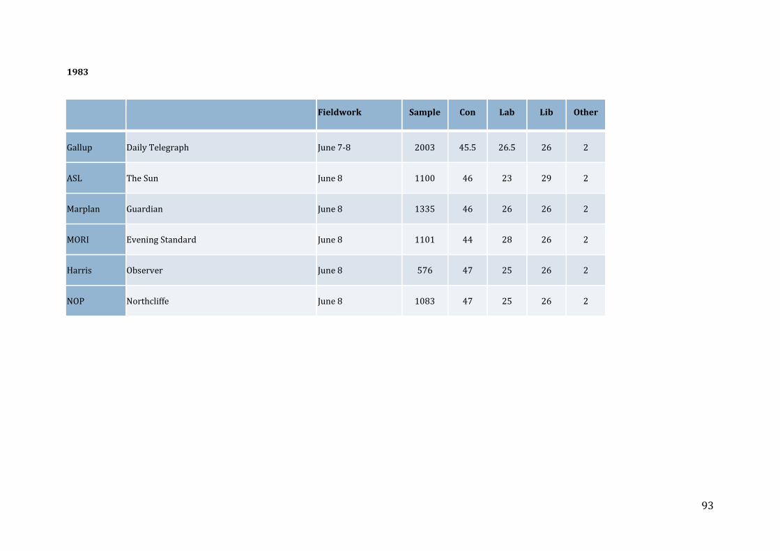
93
1983
Fieldwork Sample Con Lab Lib Other
Gallup Daily Telegraph June 7-8 2003 45.5 26.5 26 2
ASL The Sun June 8 1100 46 23 29 2
Marplan Guardian June 8 1335 46 26 26 2
MORI Evening Standard June 8 1101 44 28 26 2
Harris Observer June 8 576 47 25 26 2
NOP Northcliffe June 8 1083 47 25 26 2

94
1979
Fieldwork Sample Con Lab Lib Other
MORI Express April 29-May 1 947 44.4 38.8 13.5 3.3
Marplan The Sun May 1 1973 45 38 14 3
Gallup Daily Telegraph May 1-2 2348 43 41 13.5 2.5
MORI Evening Standard May 2 1089 45 37 15 3
NOP Daily Mail May 1-2 1069 46 39 12.5 2.5

95
1974-October
Fieldwork Sample Con Lab Lib Other
NOP Daily Mail October 2-5 1978 31 45.5 19.5 4
Gallup Daily Telegraph October 3-7 954 36 41.5 19 3.5
Marplan The Sun October 8 1024 33.3 43.8 19.5
ORC The Times October 8 446 35 44 17 3
Harris Daily Express October 5-9 678 34.6 43 19.3 3.1
ORC Evening Standard October 5-9 1071 34.4 41.8 19.4 4.4
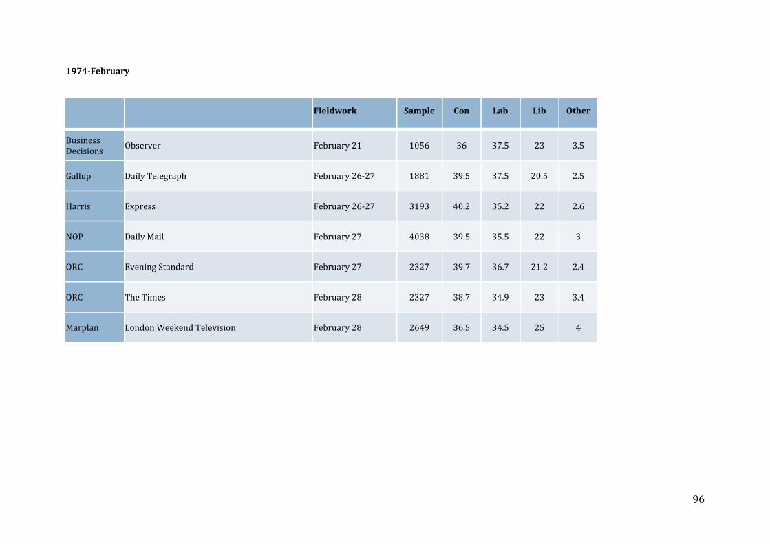
96
1974-February
Fieldwork Sample Con Lab Lib Other
Business Decisions
Observer February 21 1056 36 37.5 23 3.5
Gallup Daily Telegraph February 26-27 1881 39.5 37.5 20.5 2.5
Harris Express February 26-27 3193 40.2 35.2 22 2.6
NOP Daily Mail February 27 4038 39.5 35.5 22 3
ORC Evening Standard February 27 2327 39.7 36.7 21.2 2.4
ORC The Times February 28 2327 38.7 34.9 23 3.4
Marplan London Weekend Television February 28 2649 36.5 34.5 25 4

97
1970
Fieldwork Sample Con Lab Lib Other
Gallup Daily Telegraph June 14-16 2190 42 49 7.5 1.5
NOP Daily Mail June 12-16 1562 44.1 48.1 6.4 1.3
Marplan The Times June 11-14 2267 41.5 50.2 7 1.3
Harris Daily Express n/a 2661 46 48 5 1
ORC Evening Standard June 13-17 1840 46.5 45.5 6.5 1.5

98
1966
Fieldwork Sample Con Lab Lib Other
NOP Daily Mail March 27-29 1693 41.6 50.6 7.4 0.4
Gallup Daily Telegraph March 24-28 n/a 40 51 8 1
Daily Express - n/a n/a 37.4 54.1 7.7 0.8
Research Services
Observer n/a n/a 41.6 49.7 8.3 0.4

99
1964
Fieldwork Sample Con Lab Lib Other
Research Services
Observer n/a n/a 45 46 9 0
NOP Daily Mail October 9–13 1179 44.3 47.4 7.9 0.4
Gallup Daily Telegraph October 8–13 3829 43.5 46 8.5
Daily Express - n/a n/a 44.5 43.7 11 0.8
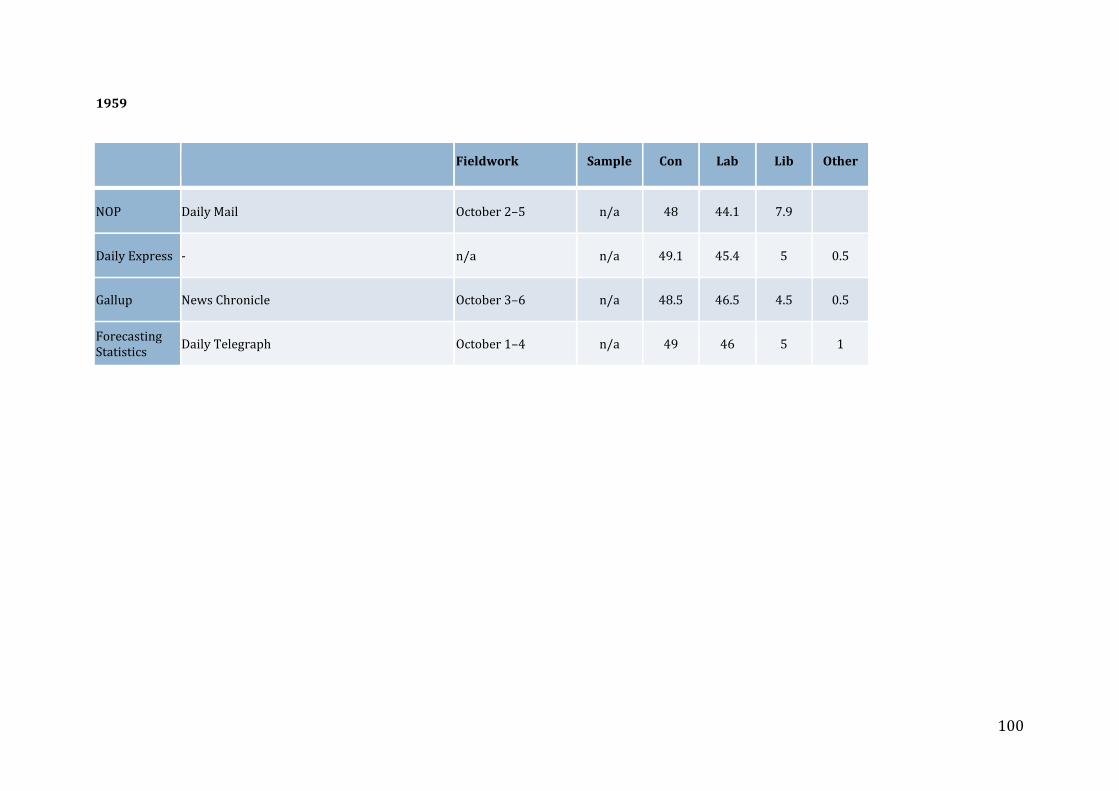
100
1959
Fieldwork Sample Con Lab Lib Other
NOP Daily Mail October 2–5 n/a 48 44.1 7.9
Daily Express - n/a n/a 49.1 45.4 5 0.5
Gallup News Chronicle October 3–6 n/a 48.5 46.5 4.5 0.5
Forecasting Statistics
Daily Telegraph October 1–4 n/a 49 46 5 1
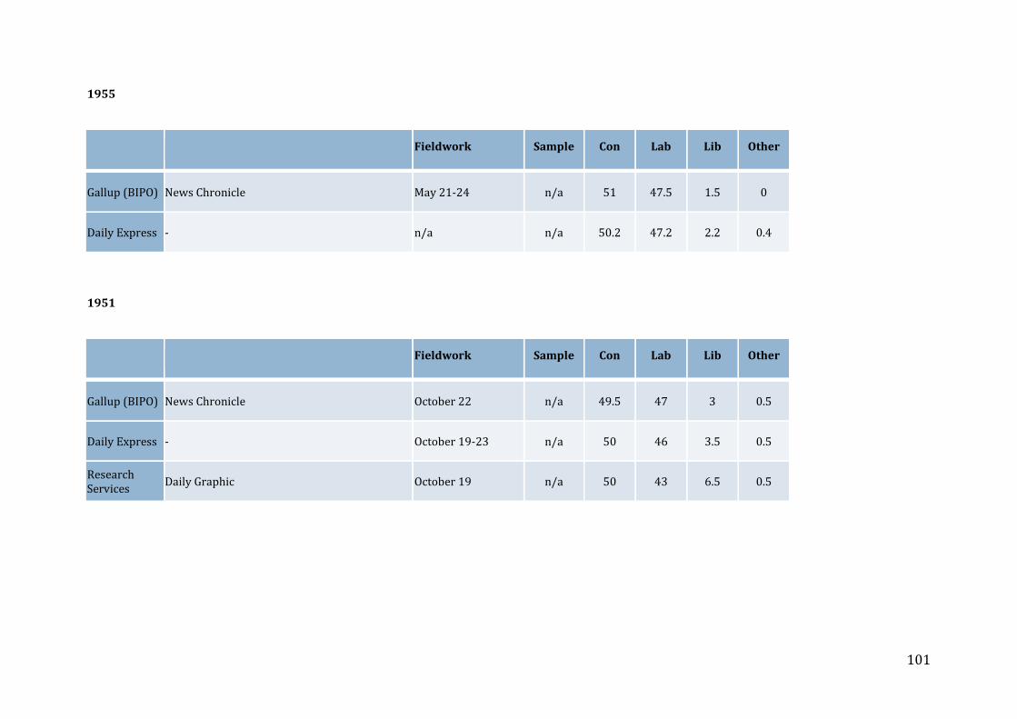
101
1955
Fieldwork Sample Con Lab Lib Other
Gallup (BIPO) News Chronicle May 21-24 n/a 51 47.5 1.5 0
Daily Express - n/a n/a 50.2 47.2 2.2 0.4
1951
Fieldwork Sample Con Lab Lib Other
Gallup (BIPO) News Chronicle October 22 n/a 49.5 47 3 0.5
Daily Express - October 19-23 n/a 50 46 3.5 0.5
Research Services
Daily Graphic October 19 n/a 50 43 6.5 0.5

102
1950
Fieldwork Sample Con Lab Lib Other
Gallup (BIPO) News Chronicle February 17–20 n/a 43.5 45 10.5 1
Daily Express - February 17–21 n/a 44.5 44 11 0.5
Daily Mail - February 5–11 n/a 45.5 42.5 12
1945
Fieldwork Sample Con Lab Lib Other
Gallup News Chronicle June 24-27 n/a 41 47 10.5 1.5
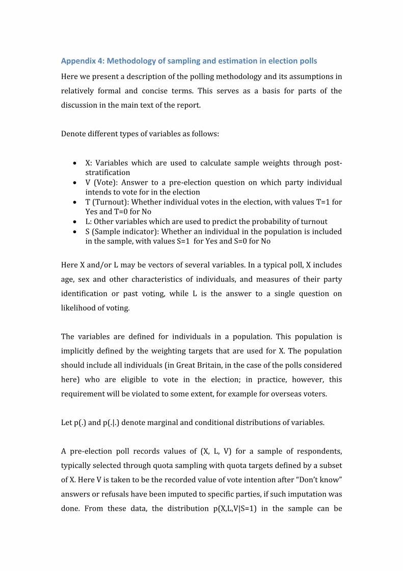
Appendix 4: Methodology of sampling and estimation in election polls
Here we present a description of the polling methodology and its assumptions in
relatively formal and concise terms. This serves as a basis for parts of the
discussion in the main text of the report.
Denote different types of variables as follows:
X: Variables which are used to calculate sample weights through post-stratification
V (Vote): Answer to a pre-election question on which party individual intends to vote for in the election
T (Turnout): Whether individual votes in the election, with values T=1 for Yes and T=0 for No
L: Other variables which are used to predict the probability of turnout S (Sample indicator): Whether an individual in the population is included
in the sample, with values S=1 for Yes and S=0 for No
Here X and/or L may be vectors of several variables. In a typical poll, X includes
age, sex and other characteristics of individuals, and measures of their party
identification or past voting, while L is the answer to a single question on
likelihood of voting.
The variables are defined for individuals in a population. This population is
implicitly defined by the weighting targets that are used for X. The population
should include all individuals (in Great Britain, in the case of the polls considered
here) who are eligible to vote in the election; in practice, however, this
requirement will be violated to some extent, for example for overseas voters.
Let p(.) and p(.|.) denote marginal and conditional distributions of variables.
A pre-election poll records values of (X, L, V) for a sample of respondents,
typically selected through quota sampling with quota targets defined by a subset
of X. Here V is taken to be the recorded value of vote intention after “Don’t know”
answers or refusals have been imputed to specific parties, if such imputation was
done. From these data, the distribution p(X,L,V|S=1) in the sample can be

104
directly estimated. Turnout T is not known at the time of the poll (with the
exception of known postal voters).
The goal of a poll is to estimate p(V|T=1), i.e. the distribution of answers to the
question on intended vote among those members of the population who will
eventually turn out to vote. For meaningful interpretation of the results, it is then
further assumed that this is also a good estimate of the distribution of actual
votes cast by voters in the election. This assumption could be violated by late
swing and/or deliberate misreporting.
This target distribution can be expressed as
𝑝(𝑉|𝑇 = 1) ∝ ∑ 𝑝(𝑉|𝐿, 𝑋)𝑝(𝑇 = 1|𝑉, 𝐿, 𝑋)𝑋,𝐿 𝑝(𝐿|𝑋)𝑝(𝑋). (A4.1)
For this to be estimable from a poll sample, the following assumptions need to be
satisfied:
[Representative sampling]: 𝑝(𝑉, 𝐿|𝑋, 𝑆 = 1) = 𝑝(𝑉, 𝐿│𝑋), i.e. the joint
distribution of V and L is the same in the sample as in the population,
conditional on each level of the weighting variables X. This also implies
that 𝑝(𝑉|𝐿, 𝑋, 𝑆 = 1)𝑝(𝐿|𝑋, 𝑆 = 1) = 𝑝(𝑉|𝐿, 𝑋)𝑝(𝐿|𝑋).
[Accurate turnout probability modelling]: 𝑝(𝑇 = 1|𝑉, 𝐿, 𝑋) is known, i.e.
it is known how the probability of turnout depends on (V,L,X) in the
population. In practice this means that a sufficiently accurate estimate of
this relationship needs to be available. This estimate cannot come from
the poll sample itself, because values of T are not known for all
respondents at the time of the poll.
Let 𝑖 = 1, … , 𝑛 index the respondents in the poll. In the first stage of the
estimation we use a set of target distributions (derived from the population
census or other sources) for at least the univariate marginal distributions in the
population for each variable in X (and possibly joint distributions of some
subsets of them, such as age by sex). Let 𝑤𝑖∗ denote poststratification weights
calculated in such a way that the weighted distributions of X in the sample match

105
these target distributions. Further, it needs to be assumed that the sample is
such that the weighted joint distribution of all of X then also matches the
population distribution, i.e. that 𝑝(𝑋|𝑆 = 1) = 𝑝(𝑋). Next, let 𝑝𝑇𝑖 denote values
of 𝑝(𝑇𝑖 = 1|𝑉𝑖, 𝐿𝑖 , 𝑋𝑖) calculated for each respondent from the assumed model for
the turnout probabilities, given their observed values of (V,L,X), and define 𝑤𝑖 =
𝑝𝑇𝑖𝑤𝑖∗. Let 𝐼(𝑉𝑖 = 𝑣) be an indicator variable for a particular party 𝑣 which is 1 if
𝑉𝑖 = 𝑣 and 0 otherwise. An estimate of 𝑝(𝑉 = 𝑣|𝑇 = 1) calculated from the poll
sample is the weighted proportion
�̂�𝑣 =∑ 𝐼(𝑉𝑖 = 𝑣)𝑤𝑖
𝑛𝑖=1
∑ 𝑤𝑖𝑛𝑖=1
.
The estimates used for all the polls are of this form. Under the assumptions
stated above, the �̂�𝑣 give a good estimate of the distribution 𝑝(𝑉|𝑇 = 1) in the
population.55
Finally, two special cases of this methodology are worth noting:
In most of the polls in 2015, L was the answer to a question on likelihood
of voting (LTV), and most turnout models that were used assumed that
𝑝(𝑇 = 1|𝑉, 𝐿, 𝑋) = 𝑝(𝑇 = 1|𝐿). This requires that (i) sample should be
representative (given the weighting variables) in likelihood of voting (L)
and not just intended vote (V); and (ii) conditional on LTV, the probability
of turnout should not depend on the weighting variables or intended vote
(the latter is the assumption of “no differential turnout misreporting”).
In principle it is not required to use any variables in the role of 𝐿. This
would be the case if the turnout model 𝑝(𝑇 = 1|𝑉, 𝐿, 𝑋) = 𝑝(𝑇 = 1|𝑉, 𝑋)
was conditional only on weighting variables X and intended vote V (or
perhaps just X). This would avoid the requirement of needing a
representative sample of L, but could make it more difficult to satisfy the
assumption that the turnout model is correct.
55 Here we use “good” as a loose term for an estimator which could be expected to give approximately correct estimates of the true distribution. Stating this in terms of more precise criteria such as (approximate) unbiasedness or consistency would require more formal assumptions about the sampling, the turnout probability modelling and the weighting targets, which we do not attempt to articulate here.

106
Appendix 5: Wording and ordering of vote intention questions
POLLSTER SURVEY
ComRes
30th March, 5th May, 6th May (30th March excluding postal vote Qs) Age + region + income + 2010 vote choice recall + voted by post. If yes, which party, if no, intention to vote (10pt) + vote choice + to all: if voting were legal - vote intention. Q. Have you already voted in the upcoming 2015 General Election by post? Q. If yes: And which party did you vote for? Was it [ROTATE] Conservative, Labour, Liberal Democrat, [FIX] UKIP, SNP [IN SCOTLAND ONLY], Plaid Cymru [IN WALES ONLY] or some other party? Q. If no: At the [*]General Election coming up [FOR INTERVIEWS ON MAY 5TH: this Thursday, 7th May], [FOR INTERVIEWS ON MAY 6TH: tomorrow], how likely would you be to vote on a scale from 1 to 10, where 1 means you are certain NOT to vote and 10 means you are absolutely CERTAIN to vote? Q. If score 5-10 on intention to vote: At the [*]General Election coming up [FOR INTERVIEWS ON MAY 5TH: this Thursday, 7th May], [FOR INTERVIEWS ON MAY 6TH: tomorrow], will you vote [ROTATE] Conservative, Labour, Liberal Democrat, [FIX] UKIP, SNP [IN SCOTLAND ONLY], Plaid Cymru [IN WALES ONLY] or for some other party? Q. To all: If it were a legal requirement for you to vote (FOR POSTAL VOTERS: “at another General Election tomorrow,”) do you think you would probably vote [ROTATE] Conservative, Labour, Liberal Democrat, [FIX] UKIP, SNP [IN SCOTLAND ONLY], Plaid Cymru [IN WALES ONLY] or for some other party?
Opinium
.
2nd April, 28th April, 4th May Gender + age + working status + region + chief earner + vote intention (inc. would not vote) + intention to vote (4pt) + leader approval ratings + 2010 vote recall. Q. How do you plan to vote, if at all, in the general election that will take place on the 7th May? Q. And how likely are you to vote in the general election that will take place on the 7th May? Q. Thinking back to the 2010 UK general election, which, if any, of the following parties did you vote for? 7th May re-contact Intro: "Please only click 'Next' to take this survey if you have already voted, either by post or in person. If you have not voted yet, please return to this survey only after you have voted. If you do not intend to vote in this election, please do not complete this survey, and we will ask your views about why you did not vote in a separate survey. Q. How did you vote in the general election that took place today?
Panelbase
31st March, 27th April Intention to vote (10 pt) + vote intention + 2010 past vote Q. A UK Parliamentary election is due to take place on May 7th - how likely is it that you will vote in that election? Q. If scores 2 and above: Who do you currently intend to vote for? Q. Did you vote in the 2010 UK Parliamentary Election which led to David Cameron becoming Prime Minister? If so, who did you vote for? 1st May Intention to vote (10 pt) + vote intention + vote intention (if in polling booth) if undecided at prior vote intention + 2010 past vote Q. A UK Parliamentary election is due to take place on May 7th - how likely is it that you will vote in that election? Q. If scores 2 and above: Who do you currently intend to vote for?
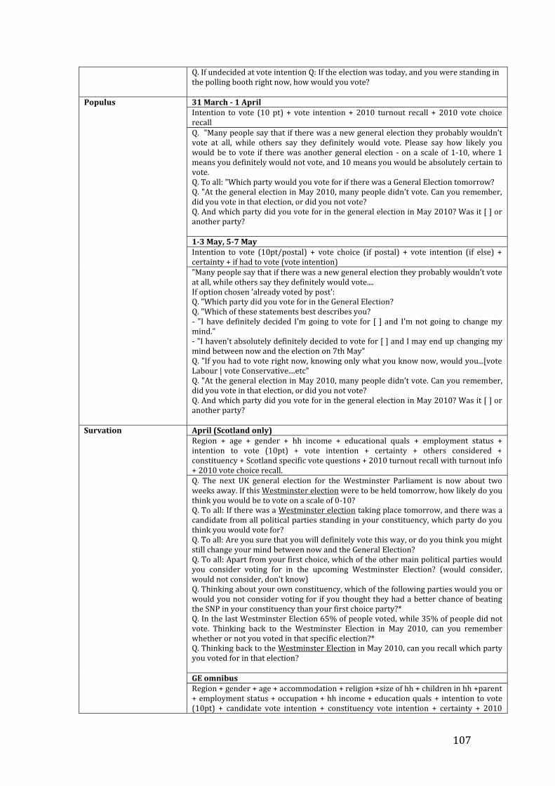
107
Q. If undecided at vote intention Q: If the election was today, and you were standing in the polling booth right now, how would you vote?
Populus
31 March - 1 April Intention to vote (10 pt) + vote intention + 2010 turnout recall + 2010 vote choice recall Q. "Many people say that if there was a new general election they probably wouldn’t vote at all, while others say they definitely would vote. Please say how likely you would be to vote if there was another general election - on a scale of 1-10, where 1 means you definitely would not vote, and 10 means you would be absolutely certain to vote. Q. To all: "Which party would you vote for if there was a General Election tomorrow? Q. "At the general election in May 2010, many people didn’t vote. Can you remember, did you vote in that election, or did you not vote? Q. And which party did you vote for in the general election in May 2010? Was it [ ] or another party? 1-3 May, 5-7 May Intention to vote (10pt/postal) + vote choice (if postal) + vote intention (if else) + certainty + if had to vote (vote intention) "Many people say that if there was a new general election they probably wouldn’t vote at all, while others say they definitely would vote.... If option chosen 'already voted by post': Q. "Which party did you vote for in the General Election? Q. "Which of these statements best describes you? - "I have definitely decided I'm going to vote for [ ] and I'm not going to change my mind." - "I haven't absolutely definitely decided to vote for [ ] and I may end up changing my mind between now and the election on 7th May" Q. "If you had to vote right now, knowing only what you know now, would you...[vote Labour | vote Conservative....etc" Q. "At the general election in May 2010, many people didn’t vote. Can you remember, did you vote in that election, or did you not vote? Q. And which party did you vote for in the general election in May 2010? Was it [ ] or another party?
Survation
April (Scotland only) Region + age + gender + hh income + educational quals + employment status + intention to vote (10pt) + vote intention + certainty + others considered + constituency + Scotland specific vote questions + 2010 turnout recall with turnout info + 2010 vote choice recall. Q. The next UK general election for the Westminster Parliament is now about two weeks away. If this Westminster election were to be held tomorrow, how likely do you think you would be to vote on a scale of 0-10? Q. To all: If there was a Westminster election taking place tomorrow, and there was a candidate from all political parties standing in your constituency, which party do you think you would vote for? Q. To all: Are you sure that you will definitely vote this way, or do you think you might still change your mind between now and the General Election? Q. To all: Apart from your first choice, which of the other main political parties would you consider voting for in the upcoming Westminster Election? (would consider, would not consider, don't know) Q. Thinking about your own constituency, which of the following parties would you or would you not consider voting for if you thought they had a better chance of beating the SNP in your constituency than your first choice party?* Q. In the last Westminster Election 65% of people voted, while 35% of people did not vote. Thinking back to the Westminster Election in May 2010, can you remember whether or not you voted in that specific election?* Q. Thinking back to the Westminster Election in May 2010, can you recall which party you voted for in that election? GE omnibus Region + gender + age + accommodation + religion +size of hh + children in hh +parent + employment status + occupation + hh income + education quals + intention to vote (10pt) + candidate vote intention + constituency vote intention + certainty + 2010

108
turnout recall. Q. The next Westminster general election is now about five weeks away. On a scale of 0-10, where 10 is certain, how certain are you to vote in the general election? Q. To all: If there was a General Election taking place tomorrow, and there was a candidate from all political parties standing in your constituency, which party do you think you would vote for?* Q. To all: The general election is on 7 May 2015. Thinking specifically about your own constituency and the parties and candidates likely to be in contention, who do you think you will vote for on 7 May? Q. To all: Are you sure that you will definitely vote this way, or do you think you might still change your mind between now and the General Election?* Q: above 2010 turnout recall with prime and 2010 vote recall. 6th May Intention to vote (10pt) + vote intention by candidates primed + combined 2010 turnout and vote choice recall Q. As you may know, the general election takes place tomorrow, Thursday 7th May. How likely are you to vote in the election on a scale of 0-10, where 10 means certain TO vote and 0 means certain NOT to vote.* Q. To all: Thinking about your [X] constituency, I'm now going to read you the names of the candidates standing [ ] Which of these candidates are you most likely to vote for in your constituency? Q. To all: Which party did you vote for in the 2010 general election, or did you not vote in that election?
TNS
Pre-election Intention to vote (4pt) + vote intention + outcome expectations + combined 2010 turnout and vote choice recall Q. Thinking about the next UK general election that will be held in May 2015, will you… Q. To all except 'definitely will not vote': Still thinking about the next UK general election, which party, if any, will you vote for in your own constituency? Q. After the next UK general election, do you think… - The Labour party will have a majority in Parliament | - The Conservative party will have a majority in Parliament | - Some other party will have a majority in Parliament | - No party will have an overall majority but Labour will be the largest party in Parliament | - No party will have an overall majority but the Conservatives will be the largest party in Parliament | Some other outcome | Don't know Q. The last General Election was held on 6th May 2010. Did you manage to vote in that General Election? Post-election Turnout + vote choice Q. The general election was held on 7th May 2015. Did you manage to vote in that general election? Q. If voted: Which party did you vote for in the general election that was held on 7th May 2015?
YouGov
30th March Vote intention (inc. will not vote) + constituency vote intention + party best on most important problem + Cons party image + Lab party image + know GE election date + certainty + intention to vote (4pt)
Q. If there were a general election held tomorrow, which party would you vote for? Q. To all: The next general election will be in May this year. Thinking specifically about your own constituency and the candidates who are likely to stand there, which party’s candidate do you think you will vote for in your own constituency at the next general election? ..... Q. From what you know, which the following is the date of the next British general election? If you don't know the date, please tick don't know rather than taking a guess. Q. The next general election is due to be held in May 2015. Have you decided definitely how you will vote then, or will you wait until nearer the time before deciding how to vote? Q. Thinking about the General Election in May, how likely are you to vote?

109
5th May, and final call survey Postal vote + vote choice if yes + vote intention if no (inc. won't vote) + constituency/candidate vote + intention to vote (10pt) + decided
Q. Thinking about the election on May 7th, do you have a postal vote? Q. If voted by post: Thinking about your own constituency and the candidates who are standing there, which party’s candidate did you vote for? Q. If not yet voted: The general election is on the 7th May / this Thursday on 7th May, which party will you vote for? Q. If not yet voted (all): Thinking specifically about your own constituency and the candidates who are likely to stand there, which party’s candidate do you think you will vote for in your own constituency at the next general election? Q. The general election will be held on May 7. On a scale of 0 (certain NOT to vote) to 10 (absolutely certain to vote), how likely are you to vote in the general election? Q. Have you decided definitely how you will vote in the election, or will you wait until nearer the time before deciding how to vote?
Squeeze Questions
These are the wordings of the questions that were administered to respondents who initially
selected the Don’t Know or Refusal options.
Ipsos-MORI: If undecided or refused: Which party are you most inclined to support? Options not
read out.
Populus: If you had to vote right now, knowing only what you know now, would you...? Vote
Labour, Vote Conservative, Vote Lib Dem, vote UKIP, Vote Green, Vote SNP, Vote Plaid Cymru,
Vote for some other party, Not vote at all.
ComRes: If it were a legal requirement for you to vote, do you think you would probably vote
Conservative, Labour, Liberal Democrat, UKIP, SNP, Plaid Cymru, or for some other party
(options not read out).
PanelBase: If the election was today, and you were standing in the polling booth right now, how
would you vote? Conservative, Labour, Liberal Democrat, SNP, UKIP, Green Party, other, would
not vote.

110
Appendix 6: Technical details of herding analysis
How much should we expect the pollsters to converge given the increases in
sample size in their final polls? The sample sizes by survey date are shown in the
figure below.
Under simple random sampling (SRS), we have clear theoretical expectations for
how these estimated variances should vary as a function of the levels of support
for the various parties and the size of the sample collected by the pollster. Let
𝑝𝑖𝑘 denote the estimated level of support in poll i for party k, and 𝜋𝑖𝑘 the
quantity in the population that 𝑝𝑖𝑘 is estimating.56 The theoretical sampling
variance of 𝑝𝑖𝑘 in a poll of sample size 𝑛𝑖 under SRS is
𝑣𝑎𝑟(𝑝𝑖𝑘) =(𝜋𝑖𝑘)(1 − 𝜋𝑖𝑘)
𝑛𝑖.
The corresponding formula for the theoretical sampling variance of the
estimated difference in level of support between two parties, in this case the
Conservatives and Labour, is:
56 This is the true level of support at the time of the poll if 𝑝𝑖𝑘 is a consistent estimate of the true support, but otherwise 𝜋𝑖𝑘 may also be different from the true level of support.
Final Day in Field
Sam
ple
Siz
e
02
000
60
00
1 Apr 8 Apr 15 Apr 22 Apr 30 Apr 7 May
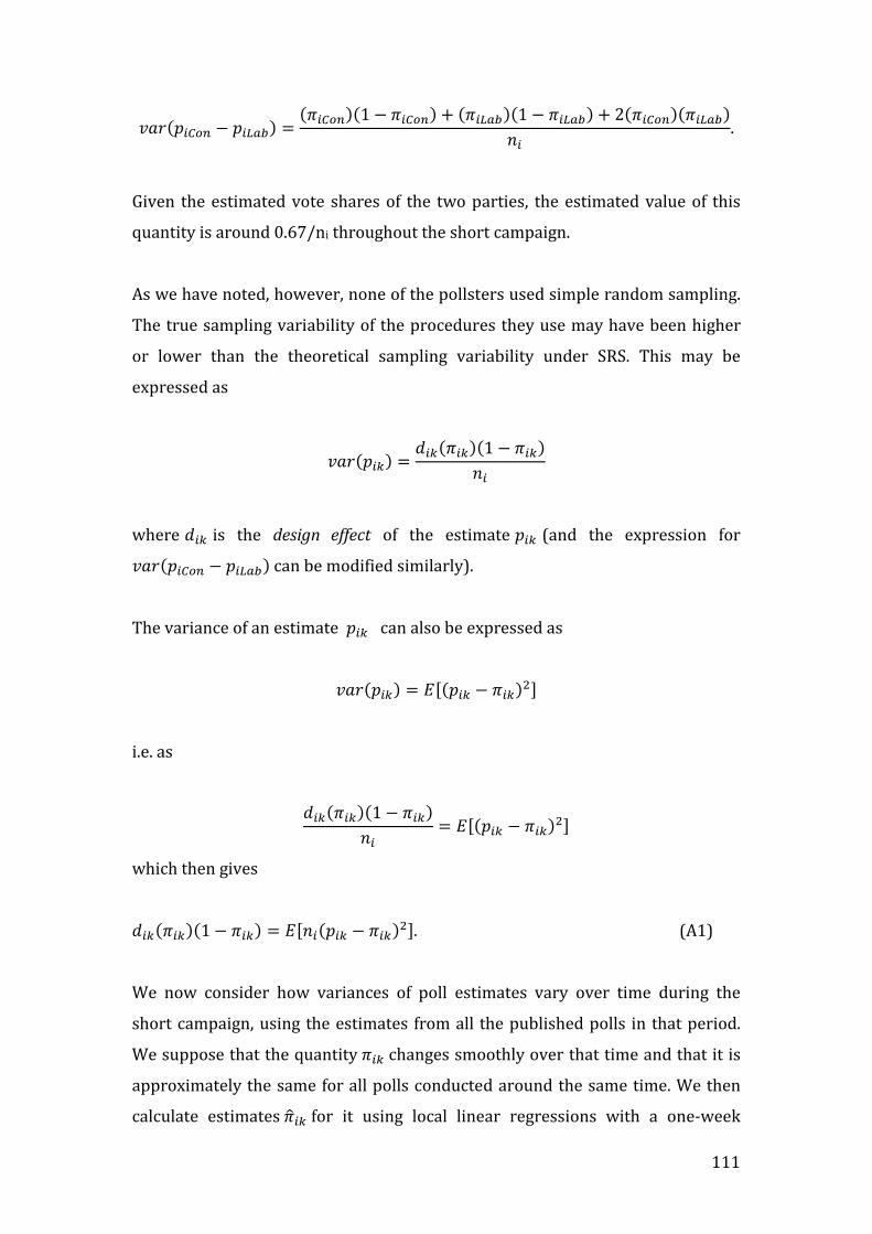
111
𝑣𝑎𝑟(𝑝𝑖𝐶𝑜𝑛 − 𝑝𝑖𝐿𝑎𝑏) =(𝜋𝑖𝐶𝑜𝑛)(1 − 𝜋𝑖𝐶𝑜𝑛) + (𝜋𝑖𝐿𝑎𝑏)(1 − 𝜋𝑖𝐿𝑎𝑏) + 2(𝜋𝑖𝐶𝑜𝑛)(𝜋𝑖𝐿𝑎𝑏)
𝑛𝑖.
Given the estimated vote shares of the two parties, the estimated value of this
quantity is around 0.67/ni throughout the short campaign.
As we have noted, however, none of the pollsters used simple random sampling.
The true sampling variability of the procedures they use may have been higher
or lower than the theoretical sampling variability under SRS. This may be
expressed as
𝑣𝑎𝑟(𝑝𝑖𝑘) =𝑑𝑖𝑘(𝜋𝑖𝑘)(1 − 𝜋𝑖𝑘)
𝑛𝑖
where 𝑑𝑖𝑘 is the design effect of the estimate 𝑝𝑖𝑘 (and the expression for
𝑣𝑎𝑟(𝑝𝑖𝐶𝑜𝑛 − 𝑝𝑖𝐿𝑎𝑏) can be modified similarly).
The variance of an estimate 𝑝𝑖𝑘 can also be expressed as
𝑣𝑎𝑟(𝑝𝑖𝑘) = 𝐸[(𝑝𝑖𝑘 − 𝜋𝑖𝑘)2]
i.e. as
𝑑𝑖𝑘(𝜋𝑖𝑘)(1 − 𝜋𝑖𝑘)
𝑛𝑖= 𝐸[(𝑝𝑖𝑘 − 𝜋𝑖𝑘)2]
which then gives
𝑑𝑖𝑘(𝜋𝑖𝑘)(1 − 𝜋𝑖𝑘) = 𝐸[𝑛𝑖(𝑝𝑖𝑘 − 𝜋𝑖𝑘)2]. (A1)
We now consider how variances of poll estimates vary over time during the
short campaign, using the estimates from all the published polls in that period.
We suppose that the quantity 𝜋𝑖𝑘 changes smoothly over that time and that it is
approximately the same for all polls conducted around the same time. We then
calculate estimates �̂�𝑖𝑘 for it using local linear regressions with a one-week

112
window and weight by the sample size of each poll. The same analysis strategy
also applies to the Conservative-Labour difference by comparison to its average.
We then assess whether any trends exist in the sample-size scaled squared
deviations using a spline regression with flexibility selected using a generalized
cross-validation criterion. In other words, we estimate in a flexible way how the
right-hand side of (A1) is observed to vary over time during the short campaign.
Because the polling averages barely shifted during the lead up to the election, the
left-hand side of equation (A1) is a constant if the average design effect of polls
across pollsters is also constant over time. This implies that the regression for
the right-hand side, that is the mean of the squared deviations of the polls from
their average, multiplied by the sample sizes of those polls, would then also be
expected to be constant even as the size of the polls changed near the election. If
it is seen to decline over time, this suggests that the variability across pollsters
has declined at the end of the campaign more than we would expect based on the
sample sizes alone.
The following plot shows this fitted curve for the mean of the squared deviations
of the polls from the polling average, scaled by their sample size, for the
Conservative-Labour difference.

113
While the downward trend in this figure is visually suggestive, it does not rise to
the level of statistical significance. An F-test of the spline regression versus the
null hypothesis of no change over time in the mean scaled squared deviation has
a p-value of 0.27.57 It is also important to note that a lack of statistical
significance in the time trend does not mean there was no time trend, rather that
we lack a sufficient number of polls with which to be certain there was such a
trend. The estimated decline in the scaled squared deviations is substantial,
from 0.54 early in the campaign period to 0.28 on the day before the election.
Two horizontal lines are also shown in the figure. The dotted line is at 0.67,
which here corresponds to simple random sampling. The dashed line is at 0.56,
which corresponds to a design effect of 0.84 in the polls. This approximate
benchmark value was obtained by calculating estimated variances for
Conservative-Labour difference, treating the polls as stratified samples stratified
by the party ID/past vote weighting cells that were used by each pollster (and
with unequal sampling probabilities implied by their final weights). The average
design effect from this calculation across the final polls for the nine pollsters is
0.84, and the average across the twenty-seven first, penultimate and final polls is
also 0.84. For the nine polls at the start of the campaign the design effect is 0.90,
and for the nine penultimate polls it is 0.78. These average design effects are
thus roughly constant, and there is no evidence of a consistent change in them
over time.
57 This is very sensitive to the exact set of polls that were reported, because the total number of polls is small.
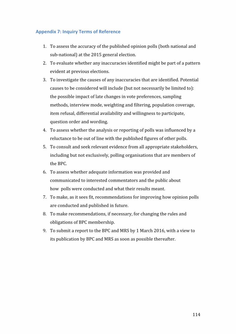
114
Appendix 7: Inquiry Terms of Reference
1. To assess the accuracy of the published opinion polls (both national and
sub-national) at the 2015 general election.
2. To evaluate whether any inaccuracies identified might be part of a pattern
evident at previous elections.
3. To investigate the causes of any inaccuracies that are identified. Potential
causes to be considered will include (but not necessarily be limited to):
the possible impact of late changes in vote preferences, sampling
methods, interview mode, weighting and filtering, population coverage,
item refusal, differential availability and willingness to participate,
question order and wording.
4. To assess whether the analysis or reporting of polls was influenced by a
reluctance to be out of line with the published figures of other polls.
5. To consult and seek relevant evidence from all appropriate stakeholders,
including but not exclusively, polling organisations that are members of
the BPC.
6. To assess whether adequate information was provided and
communicated to interested commentators and the public about
how polls were conducted and what their results meant.
7. To make, as it sees fit, recommendations for improving how opinion polls
are conducted and published in future.
8. To make recommendations, if necessary, for changing the rules and
obligations of BPC membership.
9. To submit a report to the BPC and MRS by 1 March 2016, with a view to
its publication by BPC and MRS as soon as possible thereafter.

115
Appendix 8: Conservative lead estimates by weighting cells
Figure A8.1 Conservative lead estimates by gender
note: gold = BES/BSA combined estimate; dark red = average of polls; dashed = individual polls
Figure A8.2 Conservative lead estimates by reported 2010 vote
note: gold = BES/BSA combined estimate; dark red = average of polls; dashed = individual polls