boundary layes

Prof. Nico Hotz

ME 150 – Heat and Mass Transfer

1

Laminar Boundary Layers

To calculate the convective heat transfer coefficient, we have to analyze the boundary layer close to a rigid boundary:

Conservation Equations

Specific boundary conditions are necessary to simplify these equations.

Within boundary layer: low velocities normal to wall

Outside of boundary layer: Potential flow with u∞ und T∞, no effect of viscosity

Chap. 12.2: Laminar Boundary Layers

Prof. Nico Hotz


2

2D Boundary Layer: Forced convection over plate

Flow in x-direction,

y-direction ┴ to surface,

z-direction is ∞

Boundary layers: Velocity: δ, Temperature δT

( ) ( ) ( )WWT TTTyTuyu −⋅=−=⋅== ∞∞ 99.099.0 δδ


Potential flow

Prof. Nico Hotz


3

Goal of this analysis:

Friction force on the surface (Newtonian fluid)

Heat transfer on the surface

∫ ⋅⋅=L

w dxWF0

τ

dxyuWF

yu

y

L

yw ⋅⎟⎟

⎠

⎞⎜⎜⎝

⎛

∂

∂⋅=→⎟⎟

⎠

⎞⎜⎜⎝

⎛

∂

∂⋅=

==∫

000

µµτ

∫ ⋅⋅ʹ′ʹ′=L

w dxWqq0

dxyTWkq

yTkq

y

L

y

⋅⎟⎟⎠

⎞⎜⎜⎝

⎛

∂

∂⋅−=⎟⎟

⎠

⎞⎜⎜⎝

⎛

∂

∂⋅−=ʹ′ʹ′

==∫

000


Prof. Nico Hotz


4

Laminar Boundary Layers: Solving the governing equations with three different methods: -  Order of Magnitude Method (Approximation) -  Approximate Integral Method -  Exact Similarity Method


Prof. Nico Hotz


5

Governing equations:

pca

yT

xTa

yTv

xTu

yv

xv

yP

yvv

xvu

yu

xu

xP

yuv

xuu

yv

xu

⋅=⎟⎟

⎠

⎞⎜⎜⎝

⎛

∂

∂+

∂

∂=

∂

∂+

∂

∂

=

⎪⎪

⎩

⎪⎪

⎨

⎧

⎟⎟⎠

⎞⎜⎜⎝

⎛

∂

∂+

∂

∂⋅+

∂

∂−=

∂

∂+

∂

∂

⎟⎟⎠

⎞⎜⎜⎝

⎛

∂

∂+

∂

∂⋅+

∂

∂−=

∂

∂+

∂

∂

=∂

∂+

∂

∂

ρλ

ρµ

ρ

ρ

2

2

2

2

2

2

2

2

2

2

2

2

1

1

0

E

I

K

νν

ν

Continuity

Momentum

Energy α= αk


Prof. Nico Hotz


6

∞∞∞ =∞=∞=∞∞→

====

PPTTuuy

TTvuy W

)(,)(,)(

)0(,0)0(,0)0(0

Boundary conditions for laminar boundary layers:

In the following, an estimation of phenomena in the boundary layer by analyzing orders of magnitude

Order of Magnitude Solution by Prandtl (1904)


Prof. Nico Hotz


7

Velocity Boundary Layer

vvv

UuUu

yy

LxLx

Δ→

≈Δ→

≈Δ→

≈Δ→

∞∞

?.........0:

........0:

........0:

........0:

δδ

Variables and orders of magnitudes:

LUvvv

LU

yv

xu δ

δ ∞∞ ≈=Δ→≈

Δ+→=

∂

∂+

∂

∂ 00

Approximation of order of magnitude: v

Signs are irrelevant !

Chap. 12.2.1: Velocity Boundary Layers

Prof. Nico Hotz


8

( ) ( ) yyxx PdPPdP Δ≈Δ≈

⎟⎟⎟

⎠

⎞

⎜⎜⎜

⎝

⎛

+⋅+⋅≈⋅⋅+⋅ ∞

≈

∞∞∞

∞∞ 2

0

2

1δρδ

δ ULU

LPU

LU

LUU x ν

Δ

Rearranging of pressure terms (still unknown)

x - momentum equation:

L>>δ

⎟⎟⎠

⎞⎜⎜⎝

⎛

∂

∂+

∂

∂⋅+

∂

∂−=

∂

∂+

∂

∂2

2

2

21yu

xu

xP

yuv

xuu ν

ρ


Prof. Nico Hotz


9

FrictionPressure

y

Inertia

y

LUP

LU

LUP

LLU

⋅⋅+

Δ⋅≈

⋅→⋅⋅+

Δ⋅≈⋅ ∞∞∞∞

δδρδδ

δδρδ νν 11

2

2

2

2

Similarly for y – momentum equation:

Significance of terms:

ibungDruck

x

Trägheit

ULP

LU

Re

2

2

1

12δρ∞∞

≈

⋅+⋅≈⋅ νΔ

Inertia Pressure Friction

yxyx PPP

LLP

PdyyPdx

xPdP Δ+Δ=⋅

Δ+⋅

Δ=Δ→⋅

∂

∂+⋅

∂

∂= δ

δ

Pressure terms:


Prof. Nico Hotz


10

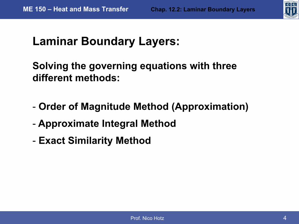
Pressure drop is caused by friction forces →

Pressure and friction terms have the same oder of magnitude

222

1δ

µδ

νρδ

νρ

∞∞∞ ⋅⋅=⋅⋅⋅≈Δ→⋅≈Δ⋅

ULULPULP

xx

LU

LUP

LUP

yy ∞∞∞ ⋅=⋅⋅≈→

⋅⋅≈⋅ µρδδρ

νν ΔΔ1

Similarly for y – component:

LUL

LUP ∞∞ ⋅+⎟

⎠

⎞⎜⎝

⎛⋅≈Δ µδ

µ2

Total pressure difference:

L>>δ xy PP ΔΔ <<


Prof. Nico Hotz


11

dxxPdPandxPP ⋅∂

∂== !)(

Conclusion:

)()( xPxP ∞=

2

21yu

dxdP

yuv

xuu

∂

∂⋅+⋅−=

∂

∂⋅+

∂

∂⋅ ∞ ν

ρ

Therefore:

x – momentum equation simplified:

very often: P1(∞) = P2(∞)

since: P1(0) = P1(∞) and P2(0) = P2(∞)

→ P1(0) = P2(0)


Prof. Nico Hotz


12

equationmomentumxyu

yuv

xuu

Continuityyv

xu

−∂

∂⋅=

∂

∂⋅+

∂

∂⋅

=∂

∂+

∂

∂

2

2

0

ν

Summary: Results of “Order of magnitude analysis “ so far:

•  Pressure term in x – momentum equation = 0

•  y – momentum equation is negligible

Relevant equations for velocity boudary layer:

∞=∞→===

Uuyvuy 00

with boundary conditions:


Prof. Nico Hotz


13

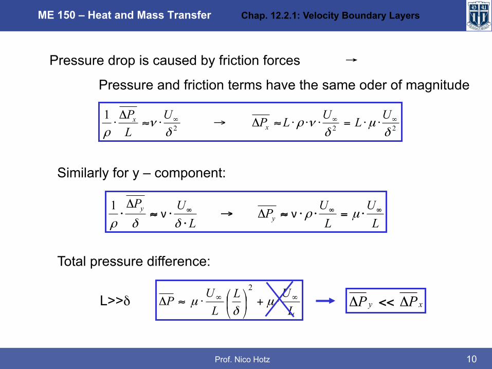
Temperature Boundary Layer

Thickness of velocity and temperature boundary layers are not identical !

δδ >>T

(1) Analysis with assumption:

Chap. 12.2.2: Temperature Boundary Layers

Prof. Nico Hotz


14

∞

∞∞

∞∞

−≈Δ→

⋅≈Δ→⋅

≈Δ→

≈Δ→

≈Δ→

∞TTTTTTL

UvL

Uv

UuUu

yy

LxLx

WW

TT

TT

.....:

........0:

........0:

........0:

........0:

δδ

δδ

Order of magnitudes for energy equation:

⎟⎟⎠

⎞⎜⎜⎝

⎛

∂

∂+

∂

∂=

∂

∂+

∂

∂2

2

2

2

yT

xT

yTv

xTu α

⎟⎟⎟⎟⎟

⎠

⎞

⎜⎜⎜⎜⎜

⎝

⎛

−+

−⋅≈

−⎟⎠

⎞⎜⎝

⎛ ⋅+−

⋅

−

∞

−

∞∞∞

∞∞

directionyinConduction

T

W

directionxinConduction

W

T

WTW TTLTTTT

LU

LTTU 22 δ

αδ

δ


L >> δT

Prof. Nico Hotz


15

2

2

yT

yTv

xTu

∂

∂⋅=

∂

∂⋅+

∂

∂⋅ α

∞=∞→

==

TTyTTy W

::0

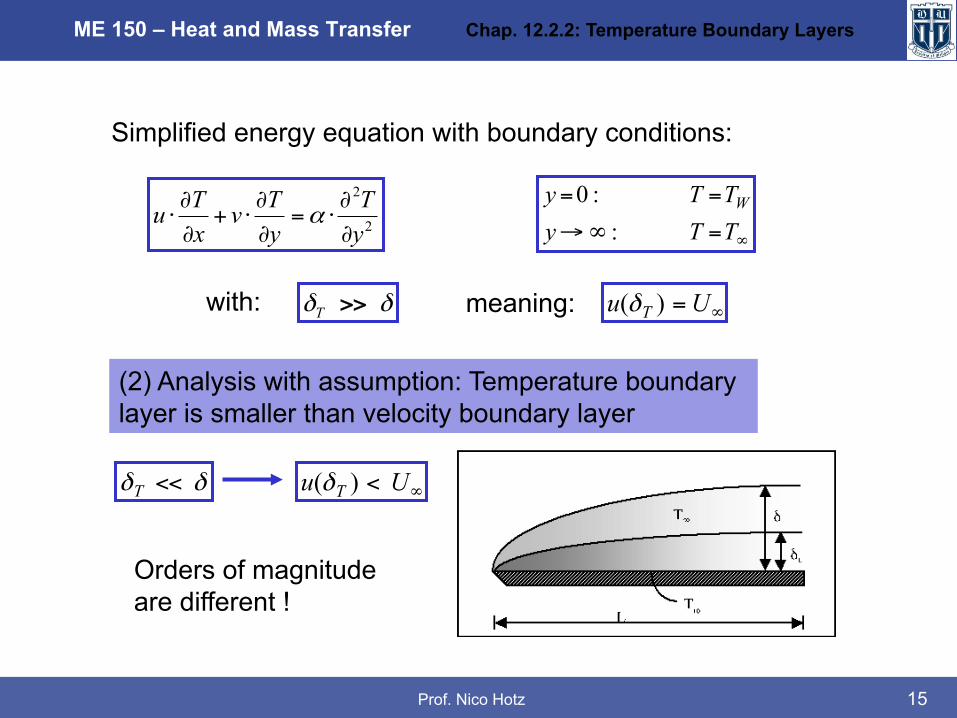
Simplified energy equation with boundary conditions:

δδ >>T ∞=Uu T )(δ

δδ <<T ∞< Uu T )(δ

with: meaning:

(2) Analysis with assumption: Temperature boundary layer is smaller than velocity boundary layer

Orders of magnitude are different !


Prof. Nico Hotz


16

For order of magnitude, we can assume a linear velocity profile

T

uUδδΔ

≈∞

δδTUu ⋅≈Δ ∞

⎟⎠

⎞⎜⎝

⎛⋅⋅≈Δ→Δ

≈Δ

→=∂

∂+

∂

∂∞ L

UvvLu

yv

xu TT

T

δδδ

δ0

Velocity component v from continuity:


Prof. Nico Hotz


17

⎟⎟⎟⎟⎟

⎠

⎞

⎜⎜⎜⎜⎜

⎝

⎛

−+

−⋅≈

−⋅⎟⎠

⎞⎜⎝

⎛⋅⎟⎠

⎞⎜⎝

⎛ ⋅+−

⋅⎟⎠

⎞⎜⎝

⎛⋅

−

∞

−

∞∞∞

∞∞

directionyinConduction

T

W

directionxinConduction

W

T

WTTWT TTLTTTT

LU

LTTU 22 δ

αδδ

δδδδ

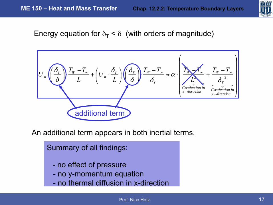
Energy equation for δT < δ (with orders of magnitude)

additional term

An additional term appears in both inertial terms.

Summary of all findings:

- no effect of pressure - no y-momentum equation - no thermal diffusion in x-direction


Prof. Nico Hotz


18

EnergyyT

yTv

xTu

Momentumxyu

yuv

xuu

Continuityyv

xu

2

2

2

2

0

∂

∂⋅=

∂

∂⋅+

∂

∂⋅

−∂

∂⋅=

∂

∂⋅+

∂

∂⋅

=∂

∂+

∂

∂

α

ν

Complete simplified equation system for boundary layer:

With boundary conditions:

yallforTTUuxTTUuyTTvuy W

∞∞

∞∞

===

=∞=∞∞→

====

0)()(:)0(0)0()0(:0


Prof. Nico Hotz


19

2

2

2

2

δδδ ∞∞

∞∞ ⋅≈⋅⎟

⎠

⎞⎜⎝

⎛ ⋅+→∂

∂⋅=

∂

∂⋅+

∂

∂⋅

UUL

ULU

yu

yuv

xuu νν

22

2 12δδ⋅≈→⋅≈⋅ ∞∞∞ νν

LUU

LU

Surface friction from order of magnitude solution

Momentum equation:

Factor 2 negligible:

( ) 21

Re21

−

≈→⎟⎟⎠

⎞⎜⎜⎝

⎛ ⋅≈

∞LLU

L δδ

νµ

ρ LULUL

⋅⋅=

⋅= ∞∞

νRe

Solving for δ:

with

Chap. 12.2.3: Surface Friction

Prof. Nico Hotz


20

( )

( ) 2122

1

21

0

Re

Re

−∞

∞

∞∞∞

∞∞

=

⋅⋅≈⋅

⋅⋅⎟

⎠

⎞⎜⎝

⎛ ⋅⋅⋅≈

⋅⋅≈⋅≈→⎟⎟⎠

⎞⎜⎜⎝

⎛

∂

∂⋅=

L

LWy

W

UUULU

LU

LUU

yu

ρρρ

νµ

µδ

µτµτ

Wall shear stress from velocity gradient:

( ) 212 Re −

∞ ⋅⋅≈ LW Uρτ

( ) 212 Re2

2−

∞ ⋅=⋅⋅≈ LffW cwithUc ρτ

Friction coefficient:


Prof. Nico Hotz


21

( ) LWUFdxWF L

L

W ⋅⋅⋅⋅→∫ ⋅⋅= −∞ 2

12

0Re~ ρτ

Friction force = Wall shear stress integrated over the entire area


Prof. Nico Hotz


22

Heat Transfer from order of magnitude solution (δ << δT)

( ) ( )22

2

T

W

T

WTW TTTTL

ULTTU

yT

yTv

xTu

δα

δδ

α ∞∞∞

∞∞

−⋅≈

−⋅⋅+

−→

∂

∂⋅=

∂

∂⋅+

∂

∂⋅

21

212

1

2 Re ⎟⎠

⎞⎜⎝

⎛⋅≈⎟⎟⎠

⎞⎜⎜⎝

⎛

⋅≈→≈

−

∞

∞

νααδ

δα

LULLU T

T

Energy equation:

Simplified and solved for δT/L:

Prandtl Number Pr αν

=Pr Peclet Number Pe PrRePe ⋅=

Chap. 12.2.4: Convective Heat Transfer

Prof. Nico Hotz


23

21

21

21

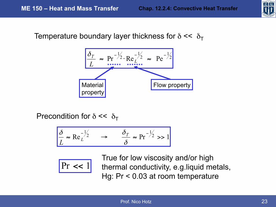
PeRePr −−−≈⋅≈ L

T

Lδ

Temperature boundary layer thickness for δ << δT

1PrRe 21

21

>>≈→≈−−

δδδ T

LL

Material property

Flow property

Precondition for δ << δT

1Pr <<True for low viscosity and/or high thermal conductivity, e.g.liquid metals, Hg: Pr < 0.03 at room temperature


Prof. Nico Hotz


24

Summary of dimensionless parameters:

Reynolds Number

Prandtl Number

Peclet Number

ForcesViscousForcesInertialLU

=⋅

= ∞

νRe

yDiffusivitThermalyDiffusivitMomentum

==ανPr

TransferHeatTransferMassLU

=⋅

=⋅= ∞

αPrRePe


Prof. Nico Hotz


25

Calculation of convective heat transfer coefficient from Fourier‘s Law:

Using the result for the temperature boundary layer:

21

21RePr LL

kh ⋅⋅≈

21

21RePrNu LL k

Lh⋅≈

⋅≡

Nusselt Number Nu as basis for calculating h:

TW

T

W

W

y kTT

TTkh

TTyTk

Tqh

δδ

≈−

−⋅

≈→−

⎟⎟⎠

⎞⎜⎜⎝

⎛

∂∂

⋅−

=Δ

ʹ′ʹ′=

∞

∞

∞

=0


Prof. Nico Hotz


26

( ) ( ) 21

21RePr LWW kTTWTThWLq ⋅⋅⋅−⋅≈−⋅⋅⋅= ∞∞

Heat flux through a rectangular area (W = width, L = length)

Note: Nusselt Number NuL leads to h averaged over 0 …. L: !

Second case: δ >> δT:

( ) ( )22

2

T

W

T

WTTWT TTTTL

ULTTU

yT

yTv

xTu

δα

δδ

δδ

δδ

α ∞∞∞

∞∞

−⋅≈

−⋅⋅⋅+

−⋅⋅→

∂

∂⋅=

∂

∂⋅+

∂

∂⋅

Energy equation (with ‘additional terms‘):

h


Prof. Nico Hotz


27

21

T

T

LU

δα

δδ

⋅≈⋅

⋅∞ ( ) 21

Re −⋅≈ LLδ

232

1

3

3

ReRe −

∞

−

⋅≈⋅

⋅≈ L

LT

ULL νααδ

21

31RePr

−−⋅≈ L

T

Lδ

1Pr 31

<<≈−

δδT

Energy equation simplified:

where

Leading to:

and results in:

Range of validity: 1Pr >


Prof. Nico Hotz


28

( ) 21

31

21

31

21

31

213

1

RePr

RePrNu

RePr

RePr

LW

L

L

LT

kTTWq

kLh

Lkh

L

⋅⋅⋅−⋅≈

⋅≈⋅

≡

⋅⋅≈

⋅≈

∞

−−δ

Summary for case 2: δ > δT

Derivation analogously to case 1:

Difference between both cases:

δ < δT δ > δT 21

Pr∝ 31

Pr∝


Prof. Nico Hotz


29

Thickness of velocity boundary layer

21

Re−≈ LLδ

Wall shear stress: 212 Re

−∞ ⋅⋅≈ LW Uρτ

Friction coefficient: 21

Re−

≈ Lfc

Friction force: 212 Re

−∞ ⋅⋅⋅⋅≈ LLWUF ρ

Summary for velocity boundary layer

(independent of δT)


Prof. Nico Hotz


30



Prof. Nico Hotz


31

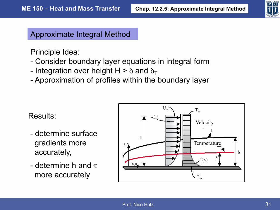
Approximate Integral Method

Principle Idea: - Consider boundary layer equations in integral form - Integration over height H > δ and δT - Approximation of profiles within the boundary layer

Results:

- determine surface gradients more accurately,

- determine h and τ more accurately

Chap. 12.2.5: Approximate Integral Method

Velocity

Temperature

Prof. Nico Hotz


32

2

22

2

2

)()(yuvu

yu

xyu

yuv

xuu

∂

∂⋅=⋅

∂

∂+

∂

∂→

∂

∂⋅=

∂

∂⋅+

∂

∂⋅ νν

continuitytodue

yv

xuu

yuv

xuu

yvu

yuv

xuuvu

yu

x0

2 2)()(

=

⎟⎟⎠

⎞⎜⎜⎝

⎛

∂

∂+

∂

∂⋅+

∂

∂⋅+

∂

∂⋅=

∂

∂⋅+

∂

∂⋅+

∂

∂⋅=⋅

∂

∂+

∂

∂

2

2

2

2

)()(yTTv

yTu

xyT

yTv

xTu

∂

∂⋅=⋅

∂

∂+⋅

∂

∂→

∂

∂⋅=

∂

∂⋅+

∂

∂⋅ αα

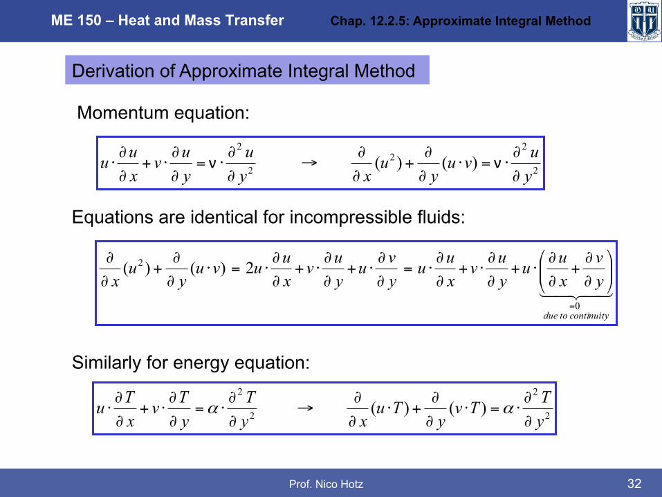
Derivation of Approximate Integral Method

Momentum equation:

Equations are identical for incompressible fluids:

Similarly for energy equation:


Prof. Nico Hotz


33

( )Hy

y

Hy

y

H

yuvudy

xdd

=

=

=

= ∂

∂⋅=⋅+⋅∫

00

0

2u ν ( )Hy

y

Hy

y

H

yTTvdyTu

xdd

=

=

=

= ∂

∂⋅=⋅+⋅⋅∫

00

0

α

( )

⎪⎪⎭

⎪⎪⎬

⎫

⎪⎪⎩

⎪⎪⎨

⎧

⎟⎟⎠

⎞⎜⎜⎝

⎛

∂

∂−⎟⎟

⎠

⎞⎜⎜⎝

⎛

∂

∂⋅=⋅−⋅+⋅

=

=

==

==∞∫0

00

00

2

yHyyHy

H

yu

yuvuvUdyu

xdd

ν

⎪⎪⎭

⎪⎪⎬

⎫

⎪⎪⎩

⎪⎪⎨

⎧

⎟⎟⎠

⎞⎜⎜⎝

⎛

∂

∂−⎟⎟

⎠

⎞⎜⎜⎝

⎛

∂

∂⋅=⋅−⋅+⋅⋅

=

=

==

=∞=∫0

00

00 yHy

WyHy

H

yT

yTTvTvdyTu

xdd

α

Integration over the boundary layer (H >> δ, δT)

Momentum equation Energy equation

Using known values at the boundary:

Momentum equation

Energy equation


Prof. Nico Hotz


34

00

2

==∞ ⎟⎟

⎠

⎞⎜⎜⎝

⎛

∂

∂⋅−=⋅+⋅∫

yHy

H

yuvUdyu

dxd ν

00 ==∞ ⎟⎟

⎠

⎞⎜⎜⎝

⎛

∂

∂⋅−=⋅+⋅⋅∫

yHy

H

yTvTdyTu

dxd

α

xu

yv

yv

xu

∂

∂−=

∂

∂→=

∂

∂+

∂

∂ 0

0

0000

=

==−=⋅=⋅−=⋅− ∫∫∫ yHy

HHH

vvdydydvdy

dxdudyu

dxd

Leading to simplified equations:

next step: determining Hyv =

using continuity:

and integrating over boundary layer:

Momentum equation Energy equation


Prof. Nico Hotz


35

0000

2 )(=

∞∞ ⎟⎟⎠

⎞⎜⎜⎝

⎛

∂

∂⋅−=⋅−⋅=⋅⋅−⋅ ∫∫∫

y

HHH

yudyUuu

dxddyu

dxdUdyu

dxd ν

0000

)(=

∞∞ ⎟⎟⎠

⎞⎜⎜⎝

⎛

∂

∂⋅−=⋅−⋅=⋅⋅−⋅⋅ ∫∫∫

y

HHH

yTdyTTu

dxddyu

dxdTdyTu

dxd

α

Combining integrals:

E

M

∞==

=

∞∞∞ ∫∫∫ ⋅−⋅+⋅−⋅=⋅−⋅

UHuu

HH

dyUuudyUuudyUuu

)()(since,0

00

)()()(

δ

δ

δ

∞==

=

∞∞∞ ∫∫∫ ⋅−⋅+⋅−⋅=⋅−⋅

THTT

HH

T

T

T

dyTTudyTTudyTTu

)()(since,0

00

)()()(

δ

δ

δ

Dividing into two parts: inside + outside of boundary layer

E

M


Prof. Nico Hotz


36

Boundary Layer Equations in Integral Form

Variables of interest

Integral equations are exact, valid as the differential equations

Still unknown: u(y), T(y)

00

00

)(

)(

=

∞

=

∞

⎟⎟⎠

⎞⎜⎜⎝

⎛

∂

∂⋅−=⋅−⋅

⎟⎟⎠

⎞⎜⎜⎝

⎛

∂

∂⋅−=⋅−⋅

∫

∫

y

y

yTadyTTu

dxd

yudyUuu

dxd

Tδ

δ

ν

α


Prof. Nico Hotz


37

δδ

<+⎟⎠

⎞⎜⎝

⎛⋅=

∞

yAyAUyu

21)(

TTw

w yByBTTTyT

δδ

<+⎟⎟⎠

⎞⎜⎜⎝

⎛⋅=

−

−

∞21

)(

∞

∞

==

==

===

TTyUuy

TTuy

TT

W

)(:)(:

)0(0)0(:0

δδ

δδ

1010

12

12

==

==

BBAA

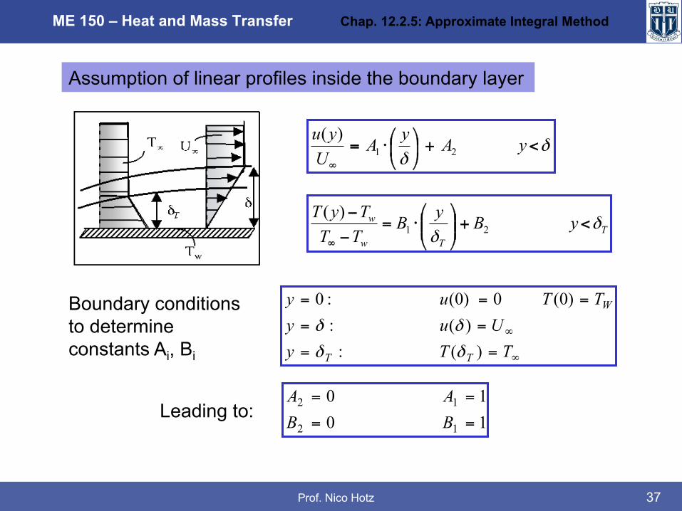
Assumption of linear profiles inside the boundary layer

Boundary conditions to determine constants Ai, Bi

Leading to:

T


Prof. Nico Hotz


38

δδδ

δ∞

∞∞∞ ⋅−=⋅⎟⎠

⎞⎜⎝

⎛−⋅⋅∫

UdyUyUyUdxd

ν0

( )δ

ζζζδ∞

−=

−=

⎪⎪

⎭

⎪⎪

⎬

⎫

⎪⎪

⎩

⎪⎪

⎨

⎧

⋅−⋅∫ Ud

dxd ν

61

1

0

1

( ) xU

xdxU

dUdx

d⋅

⋅=→⋅

⋅=⋅→

⋅=⋅

∞∞∞

ννν 62

66 2δδδ

δδ

Momentum equation: Using assumed linear profile

Dividing by U∞2, substituting with new variable:

δζ

y=

Integration over x:


Prof. Nico Hotz


39

Result: δ = f( ) x

21

Re464.3Re12:Re12 −∞

∞

⋅==⋅

=⋅⋅

= xx

x xUxwith

Ux δ

νδ

ν

( ) 212

0 Re12 xyw

UUdydu

⋅

⋅=⋅=⎟⎟

⎠

⎞⎜⎜⎝

⎛⋅= ∞∞

=

ρδ

µµτ

21

2Re577.0

21

−

∞

⋅=⋅⋅

= xw

fU

cρ

τ

Wall shear stress:

Wall shear stress coefficient:


Prof. Nico Hotz


40

Energy equation: Using assumed linear profiles

[ ] [ ]T

ww

Tw

TTdyTTyTTyUdxd T

δα

δδ

δ−

⋅−=⋅⎟⎟⎠

⎞⎜⎜⎝

⎛−−⋅−⋅⋅ ∞

∞∞∞∫0

( )T

TTTT

Ud

dxd

δα

ζζζδδ

⋅−=

⎪⎪

⎭

⎪⎪

⎬

⎫

⎪⎪

⎩

⎪⎪

⎨

⎧

⋅−⋅∞

−=

∫

61

1

0

2

1

Dividing by U∞.(T∞ -TW), using new variable:

TT

yδ

ζ =


Prof. Nico Hotz


41

31

Pr1

23

3

Pr112 −

∞

=⎟⎠

⎞⎜⎝

⎛→=⋅

⋅⋅=

δδ

δδδ TT a

Uxa

ν

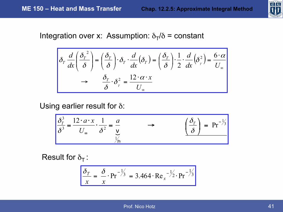
Integration over x: Assumption: δT/δ = constant

( ) ( )

∞

∞

⋅⋅=⋅→

⋅=⋅⋅⎟

⎠

⎞⎜⎝

⎛=⋅⋅⎟⎠

⎞⎜⎝

⎛=⎟⎟⎠

⎞⎜⎜⎝

⎛

Ux

Udxd

dxd

dxd

T

T

T

TTT

TTT

αδ

δδ

αδ

δδ

δδδδ

δδ

δ

12

621

2

22

Using earlier result for δ:

31

213

1PrRe464.3Pr −−−⋅⋅=⋅= x

T

xxδδ

Result for δT :


Prof. Nico Hotz


42

T

W

yW

TTkdydTkq

δ∞

=

−⋅−=⋅−=ʹ′ʹ′

0

( )∞−⋅⋅⋅⋅=ʹ′ʹ′ TTxkq wxw

31

21PrRe289.0

( ) 31

21PrRe289.0 ⋅⋅⋅=

−

ʹ′ʹ′=→−⋅=ʹ′ʹ′

∞∞ x

w

www x

kTT

qhTThq

31

21PrRe289.0Nu ⋅⋅=

⋅= xk

xα

Heat flux from Fourier‘s Law:

Using solution of δT :

Calculating convective heat transfer coefficient:

Dimensionless local Nusselt number Nu(x):


Prof. Nico Hotz


43



Prof. Nico Hotz


44

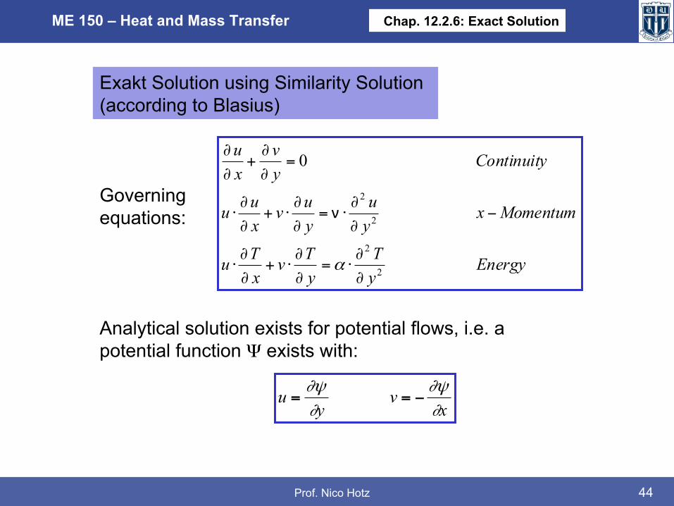
xv

yu

∂∂ψ

∂∂ψ

−==

EnergyyT

yTv

xTu

Momentumxyu

yuv

xuu

Continuityyv

xu

2

2

2

2

0

∂

∂⋅=

∂

∂⋅+

∂

∂⋅

−∂

∂⋅=

∂

∂⋅+

∂

∂⋅

=∂

∂+

∂

∂

α

ν

Exakt Solution using Similarity Solution (according to Blasius)

Governing equations:

Analytical solution exists for potential flows, i.e. a potential function Ψ exists with:

Chap. 12.2.6: Exact Solution

Prof. Nico Hotz


45

νν∞∞ ⋅

=⋅=⋅

⋅=Uxwith

xy

xUy xx ReRe 2

1η

ηddfUu ∞=

Ψ⋅⋅⋅

=

⋅=Ψ⋅∂

∂

∂

∂=

∂

∂⋅

∂

Ψ∂=

∂

Ψ∂=

∞

∞

∞

xUf

fUy

fUyy

u

ν1)(

)(

η

ηη

ηη

η

Similarity variable to transform governing equations to ODEs:

Instead of potential function, we use a function f(η):

Correlation to potential function Ψ:


Prof. Nico Hotz


46

( ) ⎟⎟⎠

⎞⎜⎜⎝

⎛⋅

⋅+

∂

∂⋅⋅⋅−=⋅⋅⋅

∂

∂−=

∂

Ψ∂−= ∞

∞∞ )(21)()( η

ηη f

xU

xfxUfxU

xxv ννν

xxU

xy

xxf

xf

⋅−=

⋅⋅−=

∂

∂

∂

∂⋅

∂

∂=

∂

∂ ∞

22)()( ηηη

ηηη

ν

( ) ( )⎟⎟⎠

⎞⎜⎜⎝

⎛−

∂

∂⋅⋅

⋅= ∞ η

ηη

ην ffxUv

21

Calculation of v from the definition of potential flow:

Derivations:

v as a function of f(η) and η:


Prof. Nico Hotz


47

3

32

2

2

2

2

2

2

2

η

η

ηη

∂

∂⋅

⋅=

∂

∂

∂

∂⋅

⋅⋅=

∂

∂

∂

∂⋅⋅

⋅−=

∂

∂

∞

∞∞

∞

fx

Uyu

fx

UUyu

fx

Uxu

ν

ν

02 2

2

3

3=

∂

∂⋅+

∂

∂⋅

ηη

fff

ηddfUu ∞=

Derivations of u necessary for momentum equation:

Momentum equation with similarity variable: ODE


Prof. Nico Hotz


48

∞→∞→

==

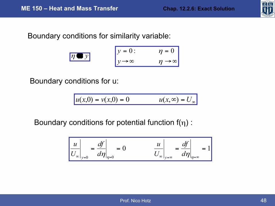
η

η

yy 0:0

∞=∞== Uxuxvxu ),(0)0,()0,(

1000

====∞=∞=∞==∞ ηη ηη d

dfUu

ddf

Uu

yy

y∝η

Boundary conditions for similarity variable:

Boundary conditions for u:

Boundary conditions for potential function f(η) :


Prof. Nico Hotz


49

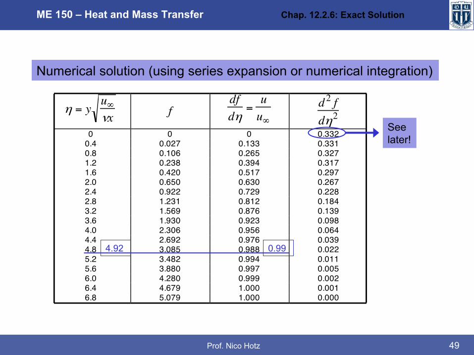
η = y u∞νx f

dfdη

=uu∞

d2 fdη2

0 0 0 0.3320.4 0.027 0.133 0.3310.8 0.106 0.265 0.3271.2 0.238 0.394 0.3171.6 0.420 0.517 0.2972.0 0.650 0.630 0.2672.4 0.922 0.729 0.2282.8 1.231 0.812 0.1843.2 1.569 0.876 0.1393.6 1.930 0.923 0.0984.0 2.306 0.956 0.0644.4 2.692 0.976 0.0394.8 3.085 0.988 0.0225.2 3.482 0.994 0.0115.6 3.880 0.997 0.0056.0 4.280 0.999 0.0026.4 4.679 1.000 0.0016.8 5.079 1.000 0.000

Numerical solution (using series expansion or numerical integration)

See later!

4.92 0.99


Prof. Nico Hotz


50

0 0.5

21

Re xxy⋅=η

1.00

2

4

6

99.092.4 ==∞U

uη

ηddf

Uu =

∞

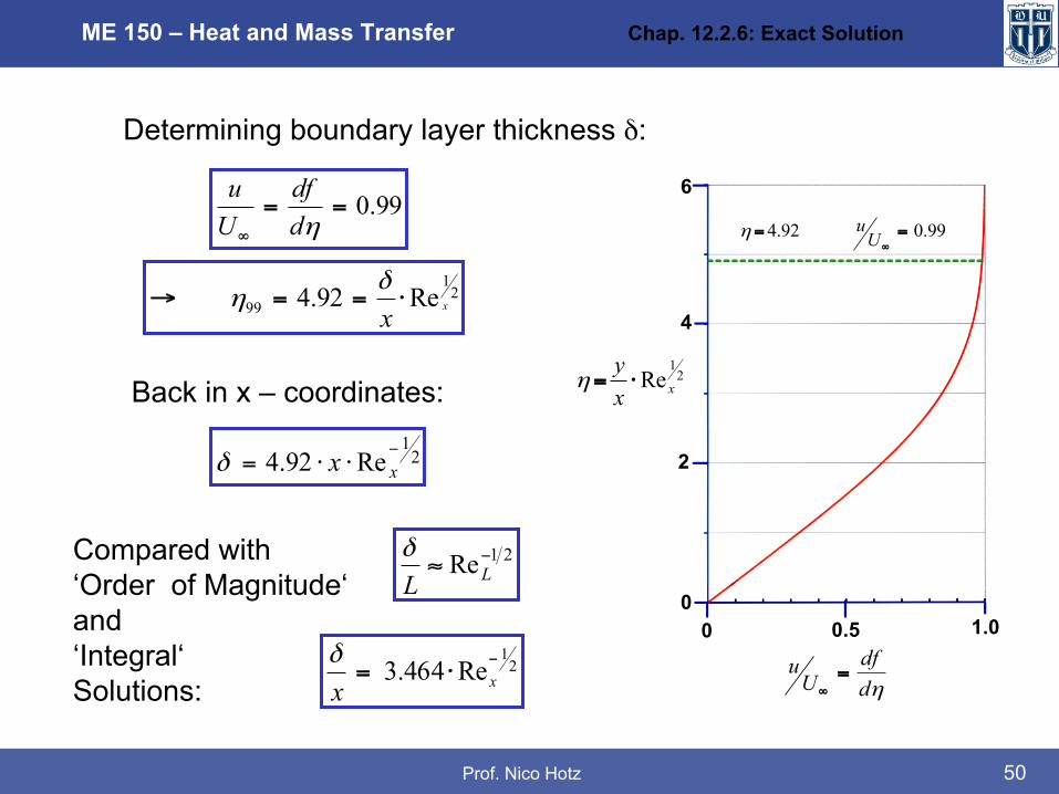
Determining boundary layer thickness δ:

99.0==∞ ηd

dfUu

21

99 Re92.4 xx⋅==→

δη

21

Re92.4 −⋅⋅= xxδ

Back in x – coordinates:

Compared with ‘Order of Magnitude‘ and ‘Integral‘ Solutions:

21Re−≈ LLδ

21

Re464.3 −⋅= xx

δ


Prof. Nico Hotz


51

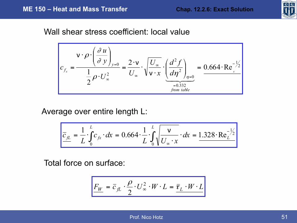
21

332.0

02

2

2

0 Re664.02

21

−

=

=

∞

∞∞

= ⋅=⎟⎟⎠

⎞⎜⎜⎝

⎛⋅

⋅⋅

⋅=

⋅

⎟⎟⎠

⎞⎜⎜⎝

⎛⋅⋅

=xx

tablefrom

yf d

fdx

UUU

yu

c η

ηρ

∂∂

ρ

νν

ν

Wall shear stress coefficient: local value

21

0 0

Re328.11664.01 −

∞

⋅=⋅⋅

⋅⋅=⋅⋅= ∫ ∫ L

L L

fxfL dxxUL

dxcL

c ν

Average over entire length L:

LWLWUcF LfLW ⋅⋅=⋅⋅⋅⋅= ∞ τρ 2

2

Total force on surface:


Prof. Nico Hotz


52

Temperature boundary layer

aTTTT

W

W ν=

−

−=

∞

Prθ

02Pr

2

2=⋅⋅+

ηθ

η

θddf

dd

1:0:0

=∞→==

θηθη

0

21

0

21

0

Re==

∞

=∞⎟⎟⎠

⎞⎜⎜⎝

⎛⋅⋅=⎟⎟

⎠

⎞⎜⎜⎝

⎛⋅⎟

⎠

⎞⎜⎝

⎛⋅

⋅=⎟⎟⎠

⎞⎜⎜⎝

⎛⋅=

−

ʹ′ʹ′=

ηη ηθ

ηθθ

dd

xk

dd

xUk

dydk

TTqh x

yW

W

ν

Definition excess temperature:

Equation to be solved (numerically):

Boundary conditions:

Results (without derivation):


Prof. Nico Hotz


53

31

0

Pr332.0:6.0Pr ⋅=⎟⎟⎠

⎞⎜⎜⎝

⎛≥

=ηηθddFor

6.0PrPr332.0Re 3121

≥⋅⋅⋅= xxkh

6.0PrPrRe332.0Nu 31

21

x ≥⋅⋅=⋅

= xkxh

Results from nume-rical solution:

Local h:

Nusselt number:

6.0Pr)(2Pr332.01)(1

0

3121

0

≥⋅=⋅⋅⋅⎟⎠

⎞⎜⎝

⎛⋅

⋅⋅=⋅⋅= ∫∫ ∞ Lhdxx

UkL

dxxhL

hLL

ν

Averaged over the range x = 0 ….. L


Prof. Nico Hotz


54

6.0PrPrRe664.02 3121 ≥⋅⋅=⋅=⋅

= LLNukLhNu

3121 PrReNu ⋅≈ L31

21

x PrRe289.0Nu ⋅⋅= x

Nusselt number averaged over range x = 0 …. L

L

xx

NuNu

Nu

⋅=≤

⋅⋅=

26.0Pr

Pr)(Re565.0 21

Numerical solution for small Prandtl numbers:

Compared with ‘Order of Magnitude‘ and ‘Integral‘ Solutions:


Prof. Nico Hotz


55

( ) 41

32

31

21

xx

Pr0468.01

PrRe3387.0Nu :100PrRePe

⎥⎦

⎤⎢⎣

⎡ +

⋅⋅=→>⋅= x

x

Semi-empirical solution (curve fitting) for any Prandtl number (Churchill and Ozoe 1973):

( ) LLhhxx

xh x Nu2Nu)(2Re

212

1

⋅=⋅=→≈≈−

Averaged values:


Prof. Nico Hotz


56

124.92 Rexx

δ −= ⋅

21

Re664.0 −⋅= xfxc

31

Pr=Tδδ

21

Re328.1 −⋅= xfxc

Heat transfer

6.0Pr >

100PrRePex >⋅= x ( ) 41

32

31

21

Pr0468.01

PrRe3387.0Nu

⎥⎦

⎤⎢⎣

⎡+

⋅⋅= x

Summary Results: Exact solution

Boundary layer thickness:

Friction coefficient:

6.0Pr < 21

Pr)(Re565.0Nu ⋅⋅=⋅

= xx kxh

31

21PrRe332.0Nu ⋅⋅=

⋅= xx k

xh


Prof. Nico Hotz


57

Documents

boundary layes