Boundary layer dynamics over London, UK, as observed using

Atmos. Chem. Phys., 11, 2111–2125, 2011www.atmos-chem-phys.net/11/2111/2011/doi:10.5194/acp-11-2111-2011© Author(s) 2011. CC Attribution 3.0 License.

AtmosphericChemistry

and Physics

Boundary layer dynamics over London, UK, as observed usingDoppler lidar during REPARTEE-II

J. F. Barlow1, T. M. Dunbar 1, E. G. Nemitz2, C. R. Wood1, M. W. Gallagher3, F. Davies4,*, E. O’Connor1,6, andR. M. Harrison 5

1Department of Meteorology, University of Reading, P.O. Box 243, Reading, RG6 6BB, UK2Centre for Ecology and Hydrology (Edinburgh), Bush Estate, Penicuik, EH26 0QB, UK3School of Earth, Atmospheric and Environmental Sciences, University of Manchester, Williamson Building, Oxford Road,Manchester, M13 9PL, UK4Room 315 Peel Building, University of Salford, The Crescent, Greater Manchester, M5 4WT, UK5School of Geography, Earth and Environmental Sciences, University of Birmingham, Birmingham, B15 2TT, UK6Finnish Meteorological Institute, P.O. Box 503, 00101 Helsinki, Finland* currently at: School of Earth and Environment, Maths/Earth and Environment Building, University of Leeds,Leeds, LS2 9JT, UK

Received: 30 April 2010 – Published in Atmos. Chem. Phys. Discuss.: 24 August 2010Revised: 20 December 2010 – Accepted: 2 February 2011 – Published: 9 March 2011

Abstract. Urban boundary layers (UBLs) can be highlycomplex due to the heterogeneous roughness and heatingof the surface, particularly at night. Due to a general lackof observations, it is not clear whether canonical models ofboundary layer mixing are appropriate in modelling air qual-ity in urban areas. This paper reports Doppler lidar obser-vations of turbulence profiles in the centre of London, UK,as part of the second REPARTEE campaign in autumn 2007.Lidar-measured standard deviation of vertical velocity aver-aged over 30 min intervals generally compared well with insitu sonic anemometer measurements at 190 m on the BTtelecommunications Tower. During calm, nocturnal peri-ods, the lidar underestimated turbulent mixing due mainlyto limited sampling rate. Mixing height derived from the tur-bulence, and aerosol layer height from the backscatter pro-files, showed similar diurnal cycles ranging from c. 300 to800 m, increasing to c. 200 to 850 m under clear skies. Theaerosol layer height was sometimes significantly different tothe mixing height, particularly at night under clear skies. Forconvective and neutral cases, the scaled turbulence profilesresembled canonical results; this was less clear for the sta-ble case. Lidar observations clearly showed enhanced mix-ing beneath stratocumulus clouds reaching down on occasionto approximately half daytime boundary layer depth. On

Correspondence to:J. F. Barlow([email protected])

one occasion the nocturnal turbulent structure was consis-tent with a nocturnal jet, suggesting a stable layer. Given thegeneral agreement between observations and canonical tur-bulence profiles, mixing timescales were calculated for pas-sive scalars released at street level to reach the BT Towerusing existing models of turbulent mixing. It was estimatedto take c. 10 min to diffuse up to 190 m, rising to between 20and 50 min at night, depending on stability. Determination ofmixing timescales is important when comparing to physico-chemical processes acting on pollutant species measured si-multaneously at both the ground and at the BT Tower duringthe campaign. From the 3 week autumnal data-set there isevidence for occasional stable layers in central London, ef-fectively decoupling surface emissions from air aloft.

1 Introduction

Understanding urban boundary layer (UBL) dynamics is par-ticularly important for accurate modelling of air quality. Dueto the difficulties in making observations in urban areas,ground-based remote sensing is becoming more important inelucidating complex UBL structure. In addition observationsof the impact of vertical dispersion in the urban boundarylayer on gases and aerosols are relatively rare. Here we reportdetailed Doppler lidar observations of central London’s UBLstructure. Observations are evaluated using in situ turbulence

Published by Copernicus Publications on behalf of the European Geosciences Union.

http://creativecommons.org/licenses/by/3.0/

2112 J. F. Barlow et al.: Boundary layer dynamics over London

measurements, compared to canonical BL results, and es-timates are made of timescales for turbulent transport fromstreet level to the top of a 190 m tall tower, the “BT Tower”.

One question is whether UBL turbulence structure is sig-nificantly different to results obtained over extensive ruralsurfaces. Roth (2000) reviewed mainly ground-based obser-vations of urban turbulence characteristics, concluding thatthere was a general agreement with similarity theories forthe urban surface layer, but due to lack of data, behaviourof the urban boundary layer above this was poorly under-stood. Various studies have used tall towers and found broadagreement with locally scaled similarity relationships, partic-ularly for complex terrain (Al-jiboori (2002), Beijing; Vesalaet al. (2008), Helsinki). Wood et al (2010) found similarbehaviour, but also estimated boundary layer height usingturbulence measurements on the 190m BT Tower in Lon-don to test mixed layer scaling. Han et al. (2009) used a250 m Tower in Tianjin to relate nocturnal pollutant levels tomixing height (MH) dynamics. Despite the micrometeoro-logical advantage of such high level measurements to assesslarge-scale urban footprints, simultaneous observation of allheights of the UBL is generally lacking – and given the po-tential complexities of UBL structure, this is particularly de-sirable.

In terms of pollution levels, mixing height is an importantcontrolling factor. Seibert (2000) reviewed methods for de-termining mixing height with respect to modelling air pol-lution as part of the COST action 710. Remote sensingmethods prove particularly useful for deriving urban mix-ing heights, being generally easier to deploy than masts, ra-diosondes (Georgoulias 2009, Thessaloniki) or tethered bal-loons, but require appropriate algorithms to derive the mixingheight (Emeis, 2008). In urban areas, various methods havebeen used, including sodar (Spanton and Williams, 1992,London); Emeis and Turk, 2004, Hannover), lidar (He etal., 2006, Beijing; Davies et al., 2007, London; Chen et al.,2001, Tsukuba) or a combination of methods including Ra-dio Acoustic Sounding System (RASS), ceilometers, windprofiles and radar (Dupont et al., 1999, Paris; Angevine et al.,2003, Nashville; Emeis et al., 2004, Hannover). Generally ithas been found that the UBL is deeper than the surroundingrural boundary layer (Angevine et al., 2003; Davies et al.,2007; Dupont et al., 1999).

Remote sensing is particularly useful in analysing verticalprofiles of turbulent mixing in the UBL. Emeis et al. (2004),Emeis et al. (2007) and Barlow et al. (2008) used acousticremote sensing to derive wind profiles and noted the sensi-tivity of the profile to underlying roughness which can behighly heterogeneous in urban areas. Use of dual Doppler li-dars (Collier et al., 2005; Newsom et al., 2005; Davies et al.,2007) can improve the accuracy in derived wind profiles andprovide dense networks of “virtual towers” (Calhoun et al.,2006, Oklahoma City), especially useful if the urban wind-field is complex due to e.g. tall buildings or changing lan-duse. Argentini et al. (1999) studied convection driven by the

relative warmth of Milan during winter-time inversion con-ditions and scaled the results using similarity theory. Morecomplex flow conditions over urban areas due to combinedeffects of the city and inversions forming in mountainous ter-rain have been studied using arrays of sodars (Piringer et al,2001, Graz) and Doppler lidar (Darby et al., 2006, Salt LakeCity).

The nocturnal urban boundary layer is particularly com-plex due to the urban heat island (UHI) delaying surfacecooling. Uno et al. (1992) observed a near-neutral ground-based layer with an elevated inversion layer at night-timeover Sapporo. Casadio et al. (1996) observed nocturnal con-vective activity using a Doppler sodar over Rome, presumedto be due to the combination of the UHI and cold air ad-vection by sea breezes over the warm urban surface. Us-ing similar equipment, Rao et al. (2002) combined Dopplersodar and Raman lidar water vapour data to estimate watervapour flux profiles over Rome over several nights. Par-ticularly large fluxes were also observed due to sea breezeadvection. Daytime sea breeze interactions with the UBLhave been studied using combinations of model and remotesensing observations (Liu et al., 2001, Hong Kong; Ferrettiet al., 2003, Rome). Lemonsu et al. (2006) found that thesea breeze, modulated by local topography, dominated overthe influence of urban surface energy balance in determiningboundary layer structure over Marseille.

The UHI also interacts with other mesoscale features atnight (e.g. regional Low Level Jets (LLJ), and mountaindrainage currents). The strong regionally formed Low LevelJet of the US mid-west was observed using Doppler sodarover Oklahoma City (Klein and Clark, 2007). Kallistratovaet al. (2009) used Doppler sodars to observe that the noctur-nal jets over Moscow were less frequent, and higher in theatmosphere than the nearby rural area. The role of katabaticflows due to the surrounding mountains in forming the jetswas acknowledged. Kolev et al. (2000, Sofia), Piringer etal., (2001, Graz) and Darby et al. (2006, Salt Lake City) allobserved complex vertical and spatial structures in nocturnalUBLs influenced by local mountainous topography.

There have been many campaigns to investigate the in-fluence of the UBL on pollutant levels using combinationsof remote sensing techniques (e.g. MEDCAPHOT-TRACEin Athens, Ziomas 1998; ECLAP in Paris, Dupont et al.,1999; ESQUIF in Paris, Menut et al., 2000; ESCOMPTEin Marseille, Cros et al., 2004 in parallel with UBL/CLU inMarseille, Mestayer et al., 2005). Banta et al. (1998) usedaeroplane based Differential Absorption Lidar (DIAL) to ob-serve ozone distributions over Nashville, combining themwith ground-based wind profiler observations of boundarylayer structure. Reitebuch et al. (2000) used Doppler so-dar profiles to observe the impact of a nocturnal jet andfrontal passage on ozone concentrations in Essen. Lidarhas been used to observe the vertical structure of particu-lates (Cooper and Eichinger 1994, Mexico City; Vakeva etal., 2000; Guinot et al., 2006, Beijing). A lidar operating at

Atmos. Chem. Phys., 11, 2111–2125, 2011 www.atmos-chem-phys.net/11/2111/2011/

J. F. Barlow et al.: Boundary layer dynamics over London 2113

wavelengths 532–1064 nm allowed Del Guasta et al. (2002)to note the correlation between aerosol mass and UBL dy-namics over Florence.

The objectives of this paper are threefold: (1) to comparethe Doppler lidar with in situ Tower turbulence observations,in order to evaluate its performance (2) to test whether theturbulent structure of the boundary layer over a large urbanarea is significantly different to canonical models, and (3)to estimate the impact of variability in turbulent structure onmixing timescales for surface-released passive scalars. Thiswork was undertaken as part of the REPARTEE project toinvestigate the chemical and dynamical processes affectingurban pollutant variability, which took place between Octo-ber 2006 and November 2007 (Harrison et al., 2011). Thepaper focuses on Doppler lidar data collected during the sec-ond Intensive Observation Period (IOP) in autumn 2007.

2 Campaign overview

2.1 Sites and instrumentation

The REPARTEE 2007 campaign ran from 15 October to 15November 2007 and the experimental aim, sites and appara-tus are fully described in Harrison et al. (2011). This paperreports only on results using the meteorological instrumenta-tion which is described here.

A 3 axis ultrasonic anemometer (R3-50, Gill Instruments,UK) and weather station (Vaisala WXT510) were installedon top of the BT Tower (lat. 51◦ 31′ 17.31′′ N, lon. 0◦ 8′

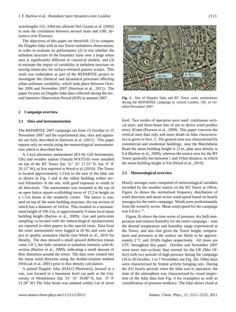
20.12′′ W), as first reported in Wood et al. (2010). The Toweris located approximately 1.2 km to the east of the lidar siteas shown in Fig. 1 and is the tallest building within sev-eral kilometres of the site, with good exposure to winds inall directions. The anemometer was mounted at the top ofan open lattice square scaffolding tower of 12.2 m height ona 1.5 m boom at the southerly corner. The lattice is situ-ated on top of the main building structure, the top section ofwhich has a diameter of 14.8 m. This resulted in a measure-ment height of 190.3 m, or approximately 9 times local meanbuilding height (Barlow et al., 2009). Gas and particulatesampling co-located with the meteorological measurementsare reported in other papers in this special issue. Data fromthe sonic anemometer were logged at 20 Hz and were sub-ject to quality assurance checks (see Wood et al., 2010 fordetails). The data showed a small upward deflection (meanvalue 5.8◦), but little variation in turbulent intensity with di-rection (Barlow et al., 2009), indicating a small amount offlow distortion around the tower. The data were rotated intothe mean wind direction using the double-rotation method(Wilczak et al. 2001) prior to flux density calculation.

A pulsed Doppler lidar (HALO Photonics), housed in avan, was located in a basement level car park at the Uni-versity of Westminster (lat. 51◦ 31′ 19.86′′ N, lon. 0◦ 9′

21.58′′ W) The lidar beam was emitted within 1 m of street

31

Figure 1. Site of Doppler lidar and BT Tower sonic anemometer during the REPARTEE

campaign in central London, UK, in October/November 2007.

Fig. 1. Site of Doppler lidar and BT Tower sonic anemometerduring the REPARTEE campaign in central London, UK, in Oc-tober/November 2007.

level. Two modes of operation were used: continuous verti-cal stare, and three-beam line of site to derive wind profilesevery 30 min (Pearson et al., 2009). This paper concerns thevertical stare data only and more detail on lidar characteris-tics is given in Sect. 3. The general area was characterised bycommercial and residential buildings: near the MaryleboneRoad the mean building height is 21 m, plan area density is0.4 (Barlow et al., 2009), whereas the source area for the BTTower generally lies between 1 and 10 km distance, in whichthe mean building height is 9 m (Wood et al., 2010).

2.2 Meteorological overview

Hourly averages were computed of meteorological variablesrecorded by the weather station on the BT Tower at 190 m.Figure 2a shows the normalised frequency distribution ofwind direction and mean sector wind-speed based on hourlyaverages for the entire campaign. Winds were predominantlyfrom the westerly sector. Mean wind-speed for the campaignwas 6.8 m s−1.

Figure 2b shows the time series of pressure, dry bulb tem-perature and relative humidity for the entire campaign – notethe diurnal temperature and humidity range experienced atthe Tower, and also that given the Tower height, tempera-tures and pressures at the surface are likely to be approxi-mately 2◦C and 20 hPa higher respectively. All times areUTC throughout this paper. October and November 2007were more anti-cyclonic than normal for the UK (Met Of-fice) with two periods of high pressure during the campaign(18 to 26 October; 1 to 7 November; see Fig. 2b). Other dayswere characterised by frontal activity bringing rain. Duringthe 432 hourly periods when the lidar was in operation, thestate of the atmosphere was characterized by visual inspec-tion of the lidar data (see Fig. 4 for examples) as well asconsideration of pressure tendency. The lidar shows cloud at

www.atmos-chem-phys.net/11/2111/2011/ Atmos. Chem. Phys., 11, 2111–2125, 2011


32

Figure 2. Meteorological data measured using Vaisala WXT510 weather station at BT Tower

during REPARTEE II. a) Mean wind-speed and direction frequency data per 45 sector

33

Figure 2. b) Time series of temperature, relative humidity and pressure data for BT Tower.

Fig. 2. Meteorological data measured using Vaisala WXT510weather station at BT Tower during REPARTEE II.(a) Mean wind-speed and direction frequency data per 45◦ sector.(b) Time seriesof temperature, relative humidity and pressure data for BT Tower.

the top of the boundary layer as high backscatter; and rainas high backscatter with downward Doppler velocity compo-nent of order 1 m s−1 in magnitude. Table 1 shows the resultof classification into categories: rain and/or frontal activity;day-time or night-time cloud; day-time or night-time “clear”.Higher level clouds not detected by the lidar will also have aninfluence on surface heating, but the structure of the bound-ary layer is determined more strongly by lower level, strati-form clouds (e.g. Lock et al., 2000). The number of “clearsky” periods was relatively high due to the dominance of highpressure periods, and of particular interest was the exception-ally large number of “clear sky” overnight periods to assessthe nocturnal radiation budget and its influence on turbulencestructure. As night-time boundary layer behaviour in urbanareas is less well studied, this data-set provides an opportu-nity to analyse this in some detail.

The turbulent flux measurements from the sonicanemometer were averaged over 30 min periods. Forthe BT Tower site, during autumn periods in 2006 and 2007,Martin (2009) showed that for particle fluxes an integration

Table 1. Frequency of periods of rain, and cloud cover estimatedfrom lidar data by day and night.

Classification Frequency (no. of hours)

Rain/frontal activity 118Day-time cloud 46Night-time cloud 93Day-time “clear” 54Night-time “clear” 121

period of 30 min leads to less than a 10% underestimatecompared to one of 60 min. Helfter et al. (2010) foundsmaller bias (<−5%) over a longer period for the same site,and concluded that 30 min averaging was a pragmatic choicecompromising between capturing all scales of turbulencecontributing to fluxes, and sub-diurnal variability. Similarreasoning is used in this study, however, it is acknowledgedthat for some periods the flux estimates presented here willbe subject to a small underestimate.

3 Doppler lidar observations

The instrument used during the campaign was a heterodyne,pulsed Doppler lidar (HALO Photonics) which had been pre-viously used at a rural site in southern England (Pearson etal., 2009), a tropical forested site (Pearson et al., 2010) andin Helsinki (Bozier et al 2007). The instrument uses 1.5 µmwavelength light of low enough energy to be eye-safe, andso is suitable for use in urban areas – other technical spec-ifications are listed in Table 2. The bias in velocity mea-surements is reported to be less than 0.02 m s−1 (Pearson etal., 2009). The lidar operated for 19 days between 25 Oc-tober and 13 November 2007 with a gate size of 30 m andintegration time of 3.6 s, giving an effective sampling rate of0.278 Hz. During the campaign it performed continuous ver-tical stare measurements of both the backscatter and verticalDoppler velocity component.

To assess accuracy of the velocity estimates the theoreticalstandard deviation for each measurement given by Rye andHardesty (1993) was used

σe =

(1v2

√2

αNp

(1+1.6α+0.4α2)

)1/2

, (1)

whereα is the ratio of the lidar detector photon count to thespeckle count,1v is the signal spectral width andNp is theaccumulated photon count, given by:

Np = SNRMn, (2)

whereM is the number of points per range gate andn is thenumber of pulses averaged.α is given by:

α =SNR

(2π)1/2(1v/B)

, (3)



Table 2. Technical specifications of Doppler lidar.

Wavelength 1.5 µm

Pulse repetition frequency 20 KHzSampling frequency 30 MHzVertical resolution 30 mIntegration time 4 s

where B is the receiver bandwidth. In this study,σ e =

0.1 m s−1 was used as a threshold above which data wererejected, which corresponds to aSNR∼ −20 dB. Backscat-ter and vertical velocity variance were then calculated over30 min averaging periods.

3.1 Comparison of lidar and sonic anemometerturbulence observations

Figure 3 shows the standard deviation of vertical velocity,σwlidar, from the lidar gate 7 (180 to 210 m), sampling at0.278 Hz plotted against the BT Tower sonic anemometerσwsonic at 190 m with sampling frequency 20 Hz, computedover 30 min periods. It can be seen that there is a correlationbut with an underestimate in slope (0.82) and considerablescatter (R2

= 0.77). At times it was observed thatσwlidarwas significantly lower thanσwsonic. It was thought that dur-ing these periods the turbulence scale is small and thus thesampling rate of the lidar is not high enough to capture allscales of turbulence contributing to the standard deviation.The size of the gate (30 m) will also limit the scale of eddieswhich the lidar can capture. To take the limited sampling rateinto account, which goes some way to enabling a comparisonbetween the instruments, Fig. 3 also shows the sonic data av-eraged to match the lidar sampling frequency. The slope hasimproved as it is closer to the 1:1 line (0.96), whilst the good-ness of fit is slightly worse (R2

= 0.73), giving confidencethat the lidar is producing similar statistics to a point mea-surement on average. Corrections, such as have been sug-gested by Hogan et al. (2009) have not been applied to thisdataset but the potential underestimate should be noted.

3.2 Derivation of heights of aerosol layers and mixingheight

Both backscatter and velocity variance data from the lidarwere used to determine three different heights pertaining tolayers in the atmosphere. The gradient in backscatterdβ/dz

was used to define the Boundary Layer top,zBL , wherethere is a very large gradient between the free atmospherewhich is relatively aerosol free compared with the pollutedBL below; and a ground-based aerosol layer depth,zAER,determined by the first exceedance of the threshold valueof backscatter gradient looking from the ground upwards(−4×10−9 m−2 sr−1). The mixing height,zMH , was defined

34

Figure 3. Scatterplot of standard deviation of vertical velocity w measured by lidar against

sonic anemometer w sampled at 20 Hz and averaged to 0.278 Hz.

Fig. 3. Scatterplot of standard deviation of vertical velocityσw

measured by lidar against sonic anemometerσw sampled at 20 Hzand averaged to 0.278 Hz.

as the height up to which a threshold ofσ 2w > 0.1 m2 s−2 was

met.Both thresholds were determined qualitatively by assess-

ing whether the magnitude and diurnal cycle of layer heightswere physically realistic and reasonably consistent from oneperiod to the next. In comparison, Pearson et al. (2010) usedσ 2

w > 0.3 m2 s−2 and first minimum in backscatter gradi-ent for a highly convective, tropical boundary layer. As itis recognized that the thresholds chosen are a little arbitrary(and probably depend on the aerosol loading), the sensitivityof derived heights to threshold criterion was tested. Given a10% perturbation in the threshold criterion forzMH , 72% ofthe values ofzMH over all 1824 periods did not change; 22%changed by 1 gate, and 6% by 2 gates or more. Similarly,for a 10% perturbation in the threshold criterion forzAER,83% did not change, 7% changed by 1 gate, and 9% changedby 2 gates or more. It was noted thatzAER was least sensi-tive to the perturbation at night, presumably because the lackof mixing sharpens the gradient in aerosol concentration andthus increases backscatter gradient.

4 Results

4.1 Boundary layer characteristic features

Figure 4 shows time series for 6 and 7 November 2007 of1 min averages of lidar data: attenuated backscatter, verticalDoppler velocity, and vertical velocity variance,σ 2

w. Thesedays were chosen as being rain-free, with no frontal activityinfluencing boundary layer state. Overlaid on the backscatterplots are estimates of aerosol layer heights, and on the vari-ance plots the mixing height is shown, all calculated accord-ing to the methods in Sect. 3.2. The height of the BT Toweris shown by a horizontal dashed line.



35

Figure 4. Doppler lidar observations of backscatter (m-1

sr-1

, log10 scale), vertical wind

velocity w (m s-1

) and variance of vertical wind velocity w2 (m

2 s

-2). Observations show 1

minute averages of 0.278 Hz data. Derived heights of boundary layer top, aerosol layer and

mixing height are also shown. Height of BT Tower (190 m) is depicted as dashed line. a) 6

November 2007

36

Figure 4. Doppler lidar observations of backscatter (m-1

sr-1

, log10 scale), vertical wind

velocity w (m s-1

) and variance of vertical wind velocity w2 (m

2 s

-2). Observations show 1

minute averages of 0.278 Hz data. Derived heights of boundary layer top, aerosol layer and

mixing height are also shown. Height of BT Tower (190 m) is depicted as dashed line. b) 7

November 2007

Fig. 4. Doppler lidar observations of backscatterβ (m−1 sr−1, log10 scale), vertical wind velocityw (m s−1) and variance of vertical windvelocityσ2

w (m2 s−2). Observations show 1 min averages of 0.278 Hz data. Derived heights of boundary layer top, aerosol layer and mixingheight are also shown. Height of BT Tower (190 m) is depicted as dashed line.(a) 6 November 2007,(b) 7 November 2007.

Various boundary layer characteristics are shown in thesetwo days. On 6 November (Fig. 4a) conditions were mostlycloud-free and mean wind-speed was 6.6 m s−1, i.e. nearcampaign average. During the overnight periods (00:00 to08:00; 21:00 to 24:00 UTC), distinct aerosol layers devel-oped at ground level extending up to approximately 500 m.It is clear that turbulent mixing is confined to a layer near theground. The Monin-Obukhov stability parameterz− zd/L

(wherezd ∼4.3 m was estimated for this part of London by

Wood et al., 2010) was determined locally at the BT Towerat 190 m and increased steadily from approximately 0.3 to1.5 between 00:00 and 07:00, showing stable conditions atthat height. Hygrosocopic aerosol particles may also havebeen growing due to increasing relative humidity as the aircooled, leading to enhanced backscatter. After sunrise at07:01, the aerosol layer broke down at approximately 08:30,as the convective boundary layer started to grow, mixingand diluting aerosols upward through its depth: changes in



backscatter intensity could also be due to changed particlecomposition and size distribution, e.g. as traffic and buildingsource activities increased. From the variance time series, itcan be seen that the ground based overnight turbulent layerdecreased in height, with the development of a band of weakturbulence between c. 300 and 500 m between 04:30 and09:00. These signatures may correspond to stable conditionsnear the ground, with turbulence generation in the high-shearvicinity of a nocturnal jet towards the top of a NocturnalBoundary Layer (NBL) – these hypotheses are explored inSect. 4.3 where individual profiles are scaled and comparedwith other similarity results.

The onset of convective mixing after sunrise at 07:01 isshown by regular enhancements in the up- and downdraughtsin the vertical Doppler velocity, and increased variance prop-agating upwards. The variance decreases from 16:00 on-wards (sunset was at 16:26) and only a small amount of tur-bulent mixing is observed in the lowest range gates fromthen onwards, extending up to the BT Tower from approx.22:00 onwards. In contrast, a ground-based aerosol layerforms from approx. 18:00 onwards, with a distinct layer ofdepth 400–600 m from 21:00. Whilst the aerosol and mix-ing heights are of similar height by day during the well-mixed Convective Boundary Layer (CBL), they diverge atnight which can influence transport of particulates emitted atground level up to the BT Tower, which may be “decoupled”from the surface if it sits above the turbulent layer (Dall’Ostoet al., 2010).

In contrast, 7 November 2007 (Fig. 4b) was predominantlyovercast due to a shallow layer of stratocumulus (shown byenhanced backscatter at c. 1 km) and mean wind-speed wasabove-average (7.4 m s−1). A tracer experiment took placeon this day and is reported in Martin et al. (2009). Overnight,from 00:00 onwards the aerosol layer persists but deepensand weakens from c. 04:00 onwards. A ground-based tur-bulent layer persists up to heights between 200 and 500 m,which mixes and dilutes aerosols through its depth. Daytimeconvective mixing occurred throughout the whole bound-ary layer from c. 11:00 until 15:00, and was replaced by aground-based turbulent layer, driven by wind shear. In con-trast to 6 November, the cloud layer overnight reduces radia-tive cooling, and thus the stability is likely to be near-neutraland turbulence is thus not suppressed. Another feature isa layer of mixing beneath the clouds, of depth c. 300-500m, most clearly seen during night-time periods. Such turbu-lence, driven by downward convection to due to cloud-top ra-diative cooling in shallow stratocumulus, has been observedusing Doppler lidar by Hogan et al. (2009) and could mixdown particulates persisting at higher levels which may haveundergone chemical reactions within the cloud. Numerousexamples of cloud-driven turbulent layers were observed dur-ing REPARTEE, and will be reported separately in a futurepublication.

37

Figure 5. Averages of derived boundary layer top (BL), aerosol layer (aerosol) and mixing

height (MH) for diurnal cycle during REPARTEE II. Error bars show standard error. a) all

periods.

38

Figure 5. Averages of derived boundary layer top (BL), aerosol layer (aerosol) and mixing

height (MH) for diurnal cycle during REPARTEE II. Error bars show standard error. b) clear

sky periods only.

Fig. 5. Averages of derived boundary layer top (BL), aerosol layer(aerosol) and mixing height (MH) for diurnal cycle during REPAR-TEE II. Error bars show standard error.(a) all periods,(b) clear skyperiods only.

4.2 Mixing height variability

Mixing height zMH , and aerosol layer heightzAER, andboundary layer depthzBL , based on backscatter, were deter-mined for all periods, and the mean time series are shown inFig. 5a (standard error of the mean as error bars). It can beseen thatzBL is relatively invariant and lies between 800 and1000 m. There is no significant difference betweenzAER andzMH by night; but by dayzMH appears to evolve 2–3 h ear-lier thanzAER. Note that sunrise occurred between 06:22 and07:16 during the campaign period, thus it takes c. 2 h forzMHto grow significantly after sunrise. Sunset occurs between17:09 and 16:12, when both layers are in decline at similarrates. An apparent lag was also seen on occasion by Emeisand Schafer (2006) when comparing mixing heights derivedfrom sodar and ceilometer data. The instruments were sepa-rated by 10 km, so differences in local surface energy balancecould not be ruled out in that case, however the present re-sults demonstrate the same effect, i.e. that the aerosol layerrises after the turbulent layer. A full discussion of possiblemechanisms is included in Sect. 4.4.



39

Figure 6. Scaled profiles of vertical windspeed variance. a) convective conditions

40

Figure 6. Scaled profiles of vertical windspeed variance. b) convective conditions with

rescaled height axis

41

Figure 6. Scaled profiles of vertical windspeed variance. c) near neutral conditions with

rescaled height axis.

42

Figure 6. Scaled profiles of vertical windspeed variance. c) stable conditions with rescaled

height axis.

43

Figure 6. Scaled profiles of vertical windspeed variance. d) possible nocturnal jet profile.

44

Figure 6. Scaled profiles of vertical windspeed variance. f) cloud-topped night-time profile. Fig. 6. Scaled profiles of vertical windspeed variance.(a) convective conditions.(b) convective conditions with rescaled height axis.(c)near neutral conditions with rescaled height axis.(d) stable conditions with rescaled height axis.(e) possible nocturnal jet profile.(f)cloud-topped night-time profile.

Figure 5b shows the diurnal evolution of the mean heightsof all layers for “clear sky” data (error bars indicate standarddeviation). Several features can be observed: (1) as mightbe expected, there is larger diurnal range, with deeper layersoccurring during the day through enhanced convective mix-ing, (2) from sunset (c. 17:00 onwards),zMH reduces sharply,whereas the nocturnal aerosol layer takes longer to form, (3)

later in the night (c. 00:00 onwards)zMH appears to reducewhereaszAER increases. Being careful to interpret the meanvalues from small numbers of datapoints,zMH < zAER on71% of occasions where clear sky data were available be-tween 00:00 and 09:00. In contrast, during the day (09:00to 17:00) on only 27% of occasionszMH < zAER, and in theperiod 17:00 to 00:00, 49% of occasions. So despite possible



errors in determination of the heights, there seems to be atendency during clear night-times for aerosol layers to prop-agate to higher heights than the classically defined mixingheight, whereas in day-time this tendency is reversed.

4.3 Boundary layer types and mixing profiles

In this section, vertical profiles ofσ 2wlidar during 6 and 7

November are grouped according to boundary layer state,scaled appropriately and compared with existing similarityresults. The purpose is to test whether urban boundary layersdisplay dissimilar characteristics to rural boundary layers, inparticular whether night-time stable boundary layer featurescan be observed.

Figure 6 shows the scaledσ 2w profiles for different bound-

ary layer states. All height co-ordinates have been cor-rected to allow for displacement height, i.e.z′

= z−zd . Fig-ure 6a shows the Convective Boundary Layer (CBL) dur-ing the day on 6 November, where the convective velocity

scale,w∗ =

{g/T0w′T ′zi

}1/3has been used. Surface tem-

peratureT0 has been approximated by using the BT Towermeasured sonic temperature (as this is converted to abso-lute temperature, this is an error of approximately 2%); thesurface temperature flux has been approximated by extrap-olating the BT Tower measured heat flux to the ground,w′T ′

z = w′T ′0(1−1.2z/zi), as shown by Wood et al. (2010)

to produce realistic mixed layer scaling. Mixing height,zMH ,has been used to represent inversion heightzi . Overlaid areexpressions by Lenschow et al. (1980), Sorbjan (1989), andan unstable profile used by the UK Met Office NAME dis-persion model (Webster et al., 2003), calculated using meanvalues ofu∗ andw∗ for the whole period.

It can be seen that the profiles are widely scattered, withprofiles towards mid-day (in blue) showing larger values.Possible errors in the scaling variables are now explored. Itcan be seen that the profiles tend to small values at heightsz > zMH , which may be due to a systematic underestimatein zMH . Using a definition of mixing height to be whereσ 2

w/w2∗ < 0.05, the profiles were rescaled using revised mix-

ing height,z′

MH . The resulting profiles are shown in Fig. 6b:it can be seen that scatter has been slightly reduced. It islikely that remaining scatter is partly due to undersampling ofthe temperature flux by use of 30 min averages. Nevertheless,the mean profile exhibits a shape consistent with the Sorb-jan (1989) and Lenschow et al. (1980) expressions. Wood etal. (2010) used an 18 month long dataset of BT Tower vari-ance measurements and found a peak atz ∼ 0.3zMH , whichagrees better with Lenschow et al. (1980). The unstableNAME profile (Webster et al., 2003) peaks further down dueto addition of mixing due to shear stress: this appears to over-estimate mixing near the surface.

Fig. 6c shows profiles during the daytime on 7 November.On-site observations confirmed 7 or 8 oktas of stratocumu-

lus throughout the day, and windy conditions, which tend tocreate near-neutral conditions. Scaling usingw∗ (not shown)was not successful in reducing scatter, whereasu∗ was; thisconfirms that the boundary layer was near-neutral rather thansignificantly convective. Again, the scaling variables havebeen adapted:u∗ was extrapolated from BT Tower heightto the surface usingu∗ = u∗0(1−z/zi) wherezi = zMH . Anovershoot of values forz′ > zMH was observed, similar to Fig6a, and therefore the height-scale was revised to be whereσ 2

w/u2∗ < 0.1. The resulting plot in Fig. 6c shows a good col-

lapse of profiles, particularly in the upper part of the bound-ary layer. A linear relationship fits very well (R2

= 0.97)to all but the lowest two points, similar to neutral bound-ary layer behaviour observed by Grant (1986), who observedmonotonic decrease abovez/zi∼0.2. Extrapolating the lin-ear relationship to the surface and taking the square root givesσw/u∗ ∼1.19, which is close the neutral result of 1.27± 0.26determined by Roth (2000) for a variety of urban datasets. Tosum up, the boundary layer properties appear to be close toother neutral case results; whether the lowest part of the pro-file (z′/zMH < 0.4) being constant with height is distinctlyurban is unclear.

The remaining figures depict night-time features. Fig-ure 6d shows the profiles for a “clear sky” period, from 18:30to 23:00 on 6 November. As sunset was at 16:26, a transi-tion period of 2 hours was estimated (Grant 1997) so peri-ods from that time were excluded. A similar procedure wasused to constrain mixing heights, i.e.z′

MH taken to be whereσ 2

w/u2∗ < 0.2. This produced an average change in mixing

height from 178 m to 262 m, the largest fractional change inestimated mixing height, being approximately 3 lidar gates(∼90 m). The potential underestimate of lidar measured vari-ance, as discussed in Sect. 3.1, could explain such an un-derestimate in mixing height during clear, calm night-timeperiods. Overlaid is the expression by Nieuwstadt (1984)based on stable boundary layer data at the Cabauw Towerin the Netherlands: it can be seen that the average profilefollows a similar decrease with height, but is significantlylarger. Apart from uncertainty in variance values due to the30 min averaging period, the local BT Toweru∗ value hasbeen used to scale the profiles: to produce agreement with theNieuwstadt values,u∗ would have to be increased by 20%.As the BT Tower during this period is very close to the mix-ing height, it is likely that the value is an underestimate ofu∗ within the turbulent layer – anecdotally, turbulence at thatheight was observed to quiesce strongly on such clear nights,consistent with the sensor being in the residual layer abovethe Nocturnal Boundary Layer. Barlow et al. (2009) also ob-served periods where the BT Tower measurements may havebeen decoupled from the surface. Despite these uncertaintiesin the scaling parameters, the turbulent layer does seem toexhibit a form consistent with a stable boundary layer.

Figure 6e also shows profiles for a “clear sky” night-timeperiod, but with radically different structure. The turbulent



layer at the ground is still observed, but instead of decreasingwith height above this, the turbulence increases again to apeak at approximately 2.5zMH . No corrections have been ap-plied to the height data in this case. The minimum in turbu-lence atz ∼ 1.3zMH is consistent with a nocturnal jet struc-ture, where there is least shear near the jet maximum. Bantaet al. (2006) observed very similar structure inσ u values us-ing Doppler lidar, and it is reasonable to assume thatσw willexhibit similar structure. The appearance of a jet-type struc-ture was highly unusual – this was the most prominent ex-ample, there being a much weaker, marginal case overnighton 1/2 November. Compared to the non-jet case in Fig. 6d,turbulent mixing was enhanced up to more than 5zMH .

Finally, Fig. 6f shows a cloudy night-time period on 7November. Here, the most distinctive additional feature isthe large peak inσw observed in the upper part of the profile.Scaling the height axis withzBL rather thanzMH producesbetter collapse of profiles at this height, giving a peak in tur-bulence atzBL ∼1. It should be emphasised that this heightis notionally proportional to cloud base, as the lidar signal isstrongly attenuated at greater heights within the cloud. Theprofiles thus demonstrate the increase in mixing in the upperboundary layer due to stratiform clouds which extends downto z ∼0.4 zBL , and appears to be distinct from the ground-based turbulent layer driven by wind shear. Radiative cool-ing at the top of the clouds determines the downward ex-tent of the mixing (Hogan et al., 2009). It can be seen fromFig. 4b that the backscatter is weak throughout the depth ofthe boundary layer for the same period, which is in stark con-trast to the earlier part of the night, where clear conditionsprobably led to a stable boundary layer and strong layeringof aerosols. As the wind-speed was near average during thisperiod (6.87 m s−1), this emphasises the impact of stratiformclouds at night in (a) preventing stable layers from forming,and (b) potentially contributing to mixing throughout a sig-nificant depth of the boundary layer.

4.4 Mixing timescales

One of the aims of the REPARTEE campaign was to deter-mine whether chemical transformations occur on the sametimescales as urban turbulent transport timescales. Specifi-cally, the meteorological observations are here used to esti-mate the timescale for turbulent transport from the surface upto the BT Tower where concurrent aerosol size distributionsand composition were recorded (reported elsewhere in thisissue).

Different time-scales can be defined to describe turbu-lence in the boundary layer (e.g. turbulent dissipation ratetimescale, Verver et al., 1997). The time-scale that deter-mines, for example, the potential for chemistry to occur be-tween emission at ground level and the measurement levelon the BT Tower is the average travel time of an inert scalarmolecule between these heights. The far-field Lagrangian

diffusivity for vertical turbulent transfer,K, is given by (Rau-pach, 1989):

K(z) = σ 2w(z)TL(z) (4)

whereTL is the Lagrangian timescale. If we adopt a simpleresistance analogy for exchange of scalars with a surface, andassume for simplicity that momentum and scalar exchangeare similar, then the effective aerodynamic resistancera(z)

can be calculated as (e.g. Thom, 1975):

ra(z) =

∫ z

z0

1

K(z)dz (5)

wherez0 is the roughness length. A transport timescale thattakes into account the integrated diffusivity can be defined as

τt (z) = γ ra(z)z (6)

wherez is the height up to which material is mixed, andγ isa coefficient, initially assumed to be 1.

Profiles ofσw and TL as used in the current version ofthe UK Met Office NAME dispersion model (Webster et al.,2003) were adopted here. These profiles were formulated toreflect existing experimental and theoretical results but alsoto avoid discontinuities across changes in stability (Websteret al., 2003). Calculatingσ 2

w(z) andTL(z) required surfacevalues ofH andu∗, which were estimated by extrapolatingthe local values measured at the BT Tower to the surface us-ing the method described in Sect. 4.3. Local temperaturemeasured at the BT Tower was used, as the results are rela-tively insensitive to temperature. Again, the inversion heightzi was estimated using the observed mixing height,zMH .

Figure 7a shows the transport timescaleτ t for each 30 minperiod throughout the campaign when lidar and sonic datawere available (372 periods). Also shown are the median,upper and lower quartile values for all data calculated for 3 hperiods. This period was chosen to include reasonable num-bers of data-points to provide more meaningful statistics. Itcan be seen that the most rapid transport times occur, notsurprisingly, during the daytime, with the median value forthe 12:00 to 15:00 period being 2580 s. There is a relativelysmall increase in median values at night (18:00 to 03:00)compared to day (09:00 to 15:00) of 16%. Notice, however,that much longer values occur during more stable night-timeconditions when negative buoyancy suppresses vertical mix-ing. This is more clearly seen in Fig. 7b which showsτ t ,normalised by its near-neutral value (3107 s, for|z′/L| < 0.1based on estimated surface fluxes) as a function of Monin-Obukhov stability parameterz′/L.

We next consider whether the calculated magnitude ofτ t

is indeed realistic.τ t was therefore calculated for 26 Octo-ber 2006, when a tracer release experiment was conducted atthe same location (Martin et al., 2009). Tracer was releasedfor 59 min atz = 0.39 m at a location∼1300 m upstream ofthe BT Tower. Samples were taken at various locations, in-cluding the top of the BT Tower, with a time resolution of



45

Figure 7. Transport timescale τt calculated for REPARTEE II. a) diurnal cycle throughout

campaign. Median, upper and lower quartile values calculated over 3 hour periods also

shown.

46

Figure 7. Transport timescale τt calculated for REPARTEE II. b) τt normalised by near neutral

value ( z‟/L < 0.1) as a function of Monin-Obukhov stability parameter z‟/L.

Fig. 7. Transport timescaleτ t calculated for REPARTEE II.(a) di-urnal cycle throughout campaign. Median, upper and lower quartilevalues calculated over 3 h periods also shown.(b) τ t normalisedby near neutral value (|z’/L | <0.1) as a function of Monin-Obukhovstability parameter z’/L.

9 min sampling time per bag (plus 1 min change-over time),repeated 6 times throughout the hour. A finite amount oftracer was detected at the top of the BT Tower in the firstsample for each repeated experiment, i.e. within 9 min of theinitial release. This gives an estimate of 540 s for the verticaltransport timescale. On this day the mean wind-speed was12.3 m s−1, conditions were near neutral, and assuming typ-ical values for roughness length of 0.75 m and displacementheight,zd , of 5 m, τ t was calculated to be 2654 s. This isa factor of 5 longer than the observations, suggesting thatγ

∼0.2, giving a median daytime value for the REPARTEE IIcampaign of 516 s. This result should be treated cautiouslyas only one tracer experiment has been used to determineγ ,and there is no theoretical basis for its value. However, itgives a near neutral estimate of∼10 min for turbulent trans-port by diffusion up to the BT Tower, increasing to∼20 to50 min for typical stable conditions, according to Fig. 7b.

To address the issue of non-passive scalars, thesetimescales need to be compared to relevant chemicaltimescales. One such approach is use of the dimensionless

Damkohler number which corresponds to the ratio of a givenchemical time scale and turbulent time scaleND ≡

τt

τcsuch

that if ND is <1 then there is little chemical transforma-tion during turbulent transport. Given the turbulent transporttimes up to the BT Tower, particularly at night-time, theremay be sufficient time for e.g. a strong interaction betweengaseous HNO3, NH3 and aerosol NH4NO3 which wouldproduce vertical fluxes that are strongly height dependent,putting certain experimental methodologies in doubt. Thetimescales presented here will allow better interpretation ofsuch urban aerosol composition data sets in future.

Whilst the estimated timescales do quantify the time tomix particles upwards, they do not appear to explain the ef-fect observed in Sect. 4.2, namely that the aerosol layer de-duced from backscatter rises 1–2 h after the turbulent layer:the timescales are too short, even if the layer through whichthe boundary layer grows is assumed to be stable. One hy-pothesis which will be explored in future work for the currentdata-set is that humidity significantly affected growth of hy-groscopic aerosol particles, leading to changes in backscatter(e.g. Gibert et al., 2007). Given the range of humidity expe-rienced at the BT Tower (see Fig. 2b: range from c. 50% to100%) it is likely that aerosol particles were affected by hu-midity changes, which could have led to changes in backscat-ter gradient and consequently yielded spurious aerosol layerheights.

5 Conclusions

During the second REPARTEE Intensive Observation Periodin October/November 2007 a pulsed Doppler lidar was de-ployed in vertical stare mode in central London with the aimof determining boundary layer structure and its impact onvertical mixing of passive scalars from the surface. In com-bination with a sonic anemometer deployed on the 190 mBT Tower, the 3 week long data-set allowed determinationof boundary layer depth, mixing timescales, and turbulentstructure under a wide range of stability conditions given theunusually high pressure and large number of clear sky peri-ods.

Comparison of the standard deviation of vertical velocitymeasured by the nearest lidar gate to the BT Tower heightwith sonic anemometer data showed a near one-to-one rela-tionship when the sonic data was averaged to the same sam-pling frequency as the lidar. The agreement between the in-struments was generally good but the lidar’s limited samplingfrequency (0.278 Hz) led to occasional underestimates of tur-bulent mixing especially during periods when the turbulencescales were smaller.

Lidar backscatter gradient and variance profiles were usedto determine aerosol layer,zAER, and mixing heightzMH,

respectively. Typical maximum daytimezMH ∼700–800 m,and 300–400 m at night. Under clear skies, the range in-creased to 750–850 m by day, and between 200–400 m at



night. The sensitivity of the derived heights to the thresh-old criteria was tested:zMH derived from the variance profileproved more robust. Consistent differences betweenzAERand zMH were observed, particularly during clear nights.zAER appeared to lag approximately two hours behindzMHin growth and decay, however this conclusion may be sensi-tive to the aerosol layer algorithm used and whether humid-ity profiles led to changes in backscatter due to hygroscopicaerosol growth. These results are generally in agreementwith other results (e.g. Pearson et al., 2010) in highlightingthe utility of Doppler lidars in providing a direct measure-ment of the mixing height, and the difficulties in interpretingheights derived from backscatter given its dependence on ef-fective aerosol radius as well as vertical distribution.

Qualitatively, both the backscatter and variance data showa rich variety of boundary layer structure and processes athigh spatial and temporal resolution. Quantitatively, thevertical velocity variance data for selected periods during6 and 7 November 2007 were scaled using mixing heightand eitheru∗ or w∗ as appropriate and compared with es-tablished results for convective, neutral and stable bound-ary layers. The results seemed to be insensitive to the es-timated error in mixing height, and the fluxes measured atthe BT Tower were extrapolated to the surface to provide es-timates of the scaling variables. The convective boundarylayer structure agreed reasonably well with Sorbjan (1989)and Lenschow et al. (1980)’s expressions with a large maxi-mum mid-boundary layer. Similarly, neutral boundary layerstructure was similar to Grant (1986), with a relatively deeplayer at the surface (z ≤0.4zMH) with near constant variance.Whether this can be associated with the enhanced mechanicalproduction of turbulence in a deep urban roughness sublayerrequires more detailed analysis. Collapse to stable formu-lations was less successful, although the general form wassimilar. This can be attributed to the difficulties in measur-ing variance profiles under stable conditions, and making arobust estimate of surface fluxes from the BT Tower mea-surement height of 190 m. Overall, the urban boundary layerstructure in this limited number of cases appears similar tocanonical boundary layers – a longer term data-set is clearlyrequired to test whether specific urban characteristics exist.

Interesting deviations from canonical profiles were ob-served during night-time periods. During the later part of aclear, calm night, evidence was seen for a nocturnal jet in thevariance profile. This was an unusual event, occurring onlyonce strongly during the campaign. This suggests that sta-ble layers do form over London, and can lead to decouplingof turbulence between the surface and the air above, but arerelatively rare, in agreement with the observations of Barlowet al. (2009) during the DAPPLE campaign, and Wood etal. (2010)’s analysis of 18 months of BT Tower data. Duringa cloudy night-time period, in addition to a turbulent layernear the ground, a thick layer of enhanced turbulence wasobserved below the cloud, down to a depth ofz ∼0.4zBL .This was thought to be downward convection, triggered by

stratocumulus radiative cooling at cloud top (Hogan et al.,2009). Such complex night-time turbulent structures shouldbe taken into account when considering both locally sourcedand long range transport of pollutants in urban atmospheres.

Given the general agreement between the variance profilesand existing formulations, parameterised profiles as used inthe UK Met Office’s NAME dispersion model (Webster et al.,2003) were used to calculate transport timescaleτ t from thesurface up to the BT Tower throughout the campaign. Me-dian values during the daytime were typically∼2500 s, ris-ing by∼16% at night. Comparing calculatedτt with a tracerexperiment performed during the first REPARTEE campaign(Martin et al., 2009), the estimated timescales seemed to be 5times too large. Using this “calibration”, the typical daytimetransport timescale was∼10 min, rising to between∼20 and50 min at night, depending on stability. These timescales areimportant to determine in relation to physico-chemical pro-cesses occurring on a similar timescale, such as the evapora-tion of semi-volatile ultrafine particles, a process observed inthe REPARTEE data (Dall’Osto et al., 2010).

These results show that Doppler lidars are highly usefultools in probing urban boundary layer structure. The resultsfor London show some evidence of decoupled turbulenceand aerosol layers during night-time. Measurements usingboth BT Tower sonic anemometer and Doppler lidar are con-tinuing under the EPSRC-funded Advanced Climate Tech-nology Urban Atmospheric Laboratory (ACTUAL) project(www.actual.ac.uk), and year-long observations of pollutantgases, particulates and boundary layer structure across Lon-don are planned through the NERC-funded ClearfLo project(www.clearflo.ac.uk).

Acknowledgements.This work was funded by the BOC Foundationand a NERC PhD studentship (T. Dunbar). The Salford Dopplerlidar is part of the National Centre for Atmospheric Science(NCAS) Facility for Ground-based Atmospheric Measurement(FGAM). We would particularly like to thank Guy Pearson andJustin Eacock of Halo Photonics who helped set up the lidar. Weare also grateful to the University of Westminster for offering spaceto deploy the lidar.

Edited by: W. T. Sturges

References

Al-Jiboori, M. H., Xu, Y., and Qian, Y.: Local similarity relation-ships in the urban boundary layer, Bound.-Layer Meteorol., 102,63–82, 2002.

Angevine, W. M., White, A. B., Senff, C. J., Trainer, M., Banta,R. M., and Ayoub, M. A.: Urban-rural contrasts in mixingheight and cloudiness over Nashville in 1999, J. Geophys. Res.,108(D3), 4092,doi:10.1029/2001JD001061, 2003.

Argentini, S., Mastrantonio, G., and Lena, F.: Case studies of thewintertime convective boundary-layer structure in the urban areaof Milan, Italy, Bound.-Layer Meteorol., 93(2) 253–267, 1999.


http://dx.doi.org/10.1029/2001JD001061


Banta, R. M., Senff, C. J., White, A. B., Trainer, M., McNider, R. T.,Valente, R. J., Mayor, S. D., Alvarez, R. J., Hardesty, R. M., Par-rish, D., and Fehsenfeld, F. C.: Daytime buildup and nighttimetransport of urban ozone in the boundary layer during a stagna-tion episode, J. Geophys. Res., 103(D17), 22519–22544, 1998.

Banta, R. M., Pichugina, Y. L., and Brewer, W. A., Turbulentvelocity-variance profiles in the stable boundary layer generatedby a nocturnal low-level jet, J. Atmos. Sci., 63, 2700–2719, 2006.

Barlow, J. F., Rooney, G. G., von Hunerbein, S., and Bradley, S. G.:Relating urban surface layer structure to upwind terrain for theSalford experiment (Salfex), Bound. Layer Meteorol., 127(2),173–191, 2008.

Barlow, J. F., Dobre, A., Smalley, R. J., Arnold, S. J., Tomlin, A. S.,and Belcher, S. E.: Referencing of street-level flows: results fromthe DAPPLE 2004 campaign in London, UK, Atmos. Environ.,43, 5536–5544, 2009.

Bozier, K. E., Pearson, G. N., and Collier, C. G.: Doppler lidar ob-servations of Russian forest fire plumes over Helsinki, Weather,62(8), 203–208, 2007.

Calhoun, R., Heap, R., Princevac, M., Newsom, R., Fernando, H.,and Ligon, D.: Virtual towers using coherent Doppler lidar dur-ing the Joint Urban 2003 dispersion experiment, J. Appl. Meteo-rol. Climatol., 45, 1116–1126, 2006.

Casadio, S., DiSarra, A., Fiocco, G., Fua, D., Lena, F., and Rao, M.P.: Convective characteristics of the nocturnal urban boundarylayer as observed with Doppler sodar and Raman lidar, Bound.-Layer Meteorol., 79(4), 375–391, 1996.

Chen, W. B., Kuze, H., Uchiyama, A., Suzuki, Y. and Takeuchi,N.: One-year observation of urban mixed layer characteristicsat Tsukuba, Japan using a micro pulse lidar, Atmos. Environ.,35(25), 4273–4280, 2001.

Collier, C. G., Davies, F., Bozier, K. E., Holt, A. R., Middleton,D. R., Pearson, G. N., Siemen, S., Willetts, D. V., Upton, G.J. G., and Young, R. I.: Dual-doppler lidar measurements forimproving dispersion models, B. Am. Meteorol. Soc., 86, 825–838, 2005.

Cooper, D. I. and Eichinger, W. E.: Structure of the atmospherein an urban planetary boundary-layer from lidar and radiosondeobservations, J. Geophys. Res., 99(D11), 22937–22948, 1994.

Cros, B., Durand, P., Cachier, H., Drobinski, P., Frejafon, E.,Kottmeier, C., Perros, P. E., Peuch, V. H., Ponche, J. L., Robin,D., Said, F., Toupance, G., and Wortham, H.: The ESCOMPTprogram: an overview, Atmos. Res., 69(3–4), 241–279, 2004.

Dall’Osto, M., Thorpe, A., Beddows, D. C. S., Harrison, R. M., Bar-low, J. F., Dunbar, T. M., Williams, P. I., and Coe, H.: Remark-able dynamics of nanoparticles in the urban atmosphere, Atmos.Chem. Phys. Discuss., 10, 30651–30689,doi:10.5194/acpd-10-30651-2010, 2010.

Darby, L. S., Allwine, K. J., and Banta, R. M.: Nocturnal low-leveljet in a mountain basin complex. Part II: Transport and diffusionof tracer under stable conditions, J. Appl., Meteorol. Climatol.,45(5), 740–753, 2006.

Davies, F., Middleton, D. R., and Bozier, K. E.: Urban air pollutionmodelling and measurements of boundary layer height, Atmos.Environ., 41, 4040–4049, 2007.

Del Guasta, M.: Daily cycles in urban aerosols observed in Florence(Italy) by means of an automatic 532-1064nm lidar, Atmos. En-viron., 36(17), 2853–2865, 2002.

Dupont, E., Menut, L., Carissimo, B., Pelon, J., and Flamant, P.:

Comparison between the atmospheric boundary layer in Parisand its rural suburbs during the ECLAP experiment, Atmos. En-viron., 33(6), 979–994, 1999.

Emeis, S.: Vertical wind profiles over an urban area, Meteorologis-che Zeitschrift, 13(5), 353–359, 2004.

Emeis, S. and Schafer, K.: Remote sensing methods to investi-gate boundary-layer structures relevant to air pollution in cities,Bound. Layer Meteorol., 121, 377–385, 2006.

Emeis, S. and Turk, M.: Frequency distributions of the mixingheight over an urban area from sodar data, MeteorologischeZeitschrift, 13(5), 361–367, 2004.

Emeis, S., Munkel, C., Vogt, S., Muller, W. J., and Schafer, K.: At-mospheric boundary-layer structure from simultaneous SODAR,RASS, and ceilometer measurements, Atmos. Environ. 38, 273–286, 2004.

Emeis, S., Baumann-Stanzer, K., Piringer, M., Kallistratova, M.,Kouznetsov, R., and Yushkov, V.: Wind and turbulence in theurban boundary layer – analysis from acoustic remote sensingdata and fit to analytical relations, Meteorologische Zeitschrift,16(4), 393–406, 2007.

Emeis, S., Schafer, K. and Munkel, C.: Surface-based remotesensing of the mixing-layer height – a review, MeteorologischeZeitschrift, 17(5), 621–630, 2008.

Ferretti, R., Mastrantonio, G., Argentini, S., Santoleri, R., and Vi-ola, A.: A model-aided investigation of winter thermally drivencirculation on the Italian Tyrrhenian coast: a case study, J. Geo-phys. Res., 108(D24), 4777,doi:10.1029/2003JD003424, 2003.

Georgoulias, A. K., Papanastasiou, D. K., Melas, D., Amiridis, V.,and Alexandri, G.: Statistical analysis of boundary layer heightsin a suburban environment, Meteorol. Atmos. Phys., 104(1–2),103–111, 2009.

Grant, A. L. M.: An observational study of the evening transitionboundary-layer, Q. J. Roy. Meteorol. Soc., 123, 657–677, 1997.

Grant, A. L. M.: Observations of boundary layer structure madeduring the 1981 KONTUR experiment, Q. J. Roy. Meteorol.Soc., 112, 825–841, 1986.

Guinot, B., Roger, J. C., Cachier, H., Wang, P. C., Bai, J. H., andTong, Y.: Impact of vertical atmospheric structure on Beijingaerosol distribution, Atmos. Environ., 40(27), 5167–5180, 2006.

Han, S. Q., Bian, H., Tie, X. X., Xie, Y. Y., Sun, M. L. and Liu,A. X.: Impact of nocturnal planetary boundary layer on urbanair pollutants: measurements from a 250m-tower over Tianjin,China, J. Hazardous Materials, 162(1), 264–269, 2009.

Harrison, R. M., DallOsto, M., Thorpe, A. J., Allan, J., Coe, H.,Dorsey, J., Gallagher, M., Martin, C., Whitehead, J., WilliamsP., Benton, A. K., Jones, R. L., Langridge, J., Ball, S., Lang-ford, B., Hewitt, C. N., Davison, B., Martin, D., Petersson, K.,Henshaw, S. J., White, I. R., Shallcross, D. E., Barlow, J. F., Dun-bar, T., Davies, F., and Nemitz, E. G.:Atmospheric chemistry andphysics in the atmosphere of a developed megacity (London): anoverview of the REPARTEE experiment and its conclusions, inpreparation, 2011.

He, Q. S., Mao, J. T., Chen, J. Y., and Hu, Y. Y.: Observational andmodelling studies of urban atmospheric boundary-layer heightand its evolution mechanisms, Atmos. Environ., 40(6), 1064–1077, 2006.

Helfter, C., Famulari, D., Phillips, G. J., Barlow, J. F., Wood, C. R.,Grimmond, C. S. B., and Nemitz, E.: Controls of carbon dioxideconcentrations and fluxes above central London, Atmos. Chem.


http://dx.doi.org/10.5194/acpd-10-30651-2010


http://dx.doi.org/10.1029/2003JD003424


Phys. Discuss., 10, 23739–23780,doi:10.5194/acpd-10-23739-2010, 2010.

Hogan, R. J., Grant, A. L. M., Illingworth, A. J., Pearson, G. N. andO’Connor, E. J.: Vertical velocity variance and skewness in clearand cloud-topped boundary layers as revealed by Doppler lidar,Q. J. Roy. Meteorol. Soc., 135, 635–643, 2009.

Kallistratova, M., Kouznetsov, R. D., Kuznetsov, D. D.,Kuznetsova, I. N., Nakhaev, M., and Chirokova, G.: Summer-time low-level jet characteristics measured by sodars over ruraland urban areas, Meteorologische Zeitschrift, 18(3), 289–295,2009.

Klein, P. and Clark, J. V.: Flow variability in a north Americandowntown street canyon, J. Appl. Meteorol. Climatol., 46, 851–877, 2007.

Kolev, I., Savov, P., Kaprielov, B., Parnanov, O., and Simeonov,V.: Lidar observations of the nocturnal boundary layer formationover Sofia, Bulgaria, Atmos. Environ., 34(19), 3223–3235, 2000.

Langford, B., Nemitz, E., House, E., Phillips, G. J., Famulari,D., Davison, B., Hopkins, J. R., Lewis, A. C., and Hewitt, C.N.: Fluxes and concentrations of volatile organic compoundsabove central London, UK, Atmos. Chem. Phys., 10, 627–645,doi:10.5194/acp-10-627-2010, 2010.

Lemonsu, A., Bastin, S., Masson, V., and Drobinski, P.: Verticalstructure of the urban boundary layer over Marseille under sea-breeze conditions, Bound.-Layer Meteorol., 118(3), 477–501,2006.

Lenschow, D. H., Wyngaard, J. C., and Pennell, W. T.: Mean-fieldand second moment budgets in a baroclinic, convective boundarylayer, J. Atmos. Sci. 37, 1313–1326, 1980.

Liu, H. P., Chan, J. C. L., and Cheng, A. Y. S.: Internal bound-ary layer structure under sea-breeze conditions in Hong Kong,Atmos. Environ., 35(4), 683–692, 2001.

Lock, A. P., Brown, A. R., Bush, M. R., Martin, G. M., and Smith,R. N. B.: A new boundary layer mixing scheme. Part I: schemedescription and single-column model tests, Mon. Weather Rev.,128, 3187–3199, 2000.

Martin, C. L.: Transportation and transformation of urban aerosolparticles, PhD. Thesis, University of Manchester, Manchester,UK, 2009.

Martin, D., Petersson, K. F., White, I. R., Henshaw, S. J., Nickless,G., Lovelock, A., Barlow, J. F., Dunbar, T., Wood, C. R., andShallcross, D. E.: Tracer concentration profiles measured in cen-tral London as part of the REPARTEE campaign, Atmos. Chem.Phys., 11, 227–239,doi:10.5194/acpd-11-227-2011, 2011.

Menut, L., Vautard, R., Flamant, C., Abonnel, C., Beekmann, M.,Chazette, P., Flamant, P. H., Gombert, D., Guedalia, D., Kley,D., Lefebvre, M. P., Lossec, B., Martin, D., Megie, G., Per-ros, P., Sicard, M., and Toupance, G.: Measurements and mod-elling of atmospheric pollution over the Paris area: an overviewof the ESQUIF project, Ann. Geophys., 18(11), 1467–1481,doi:10.5194/angeo-18-1467-2000, 2000.

Met Office Monthly climate summary for October 2007,http://www.metoffice.gov.uk/climate/uk/2007/october.html, last ac-cess: 18 August 2009, 2007.

Newsom, R. K., Ligon, D., Calhoun, R., Heap, R., Cregan, E.,and Princevac, M.: Retrieval of microscale wind and temper-ature fields from single- and dual-Doppler lidar data, J. Appl.,Meteorol., 44(9), 1324–1345, 2005

Nieuwstadt, F. T. M.: The turbulent structure of the stable, nocturnal

boundary layer, J. Atmos. Sci., 41(14), 2202–2216, 1984.Pearson, G. N., Davies, F., and Collier, C. G.: An analysis of the

performance of the UFAM pulsed Doppler lidar for observingthe boundary layer, J. Atmos. Ocean. Tech., 26, 240–250, 2009.

Pearson, G., Davies, F., and Collier, C.: Remote sensing of thetropical rain forest boundary layer using pulsed Doppler lidar,Atmos. Chem. Phys., 10, 5891–5901,doi:10.5194/acp-10-5891-2010, 2010.

Piringer, M. and Baumann, K.: Exploring the urban boundary layerby sodar and tethersonde, Phys. Chem. of the Earth, 26(11–12),881–885, 2001.

Rao, M. P., Casadio, S., Fiocco, G., Cacciani, M., Di Sarra, A.,Fua, D., and Castracane, P.: Estimation of atmospheric watervapour flux profiles in the nocturnal unstable urban boundarylayer with Doppler sodar and Raman lidar, Boundary-layer Me-teorol., 102(1), 39–62, 2002.

Raupach, M. R.: A practical Lagrangian method for relating scalarconcentrations to source distributions in vegetation canopies, Q.J. R. Meteorol. Soc., 115, 609–632, 1989.

Reitebuch, O., Strassburger, A., Emeis, S., and Kuttler, W.: Noc-turnal secondary ozone concentration maxima analysed by so-dar observations and surface measurements, Atmos. Environ.,34(25), 4315–4329, 2000.

Roth, M.: Review of atmospheric turbulence over cities, Q. J. Roy.Meteorol. Soc. 126, 941–990, 2000.

Rye, B. J. and Hardesty, R. M.: Discrete spectral peak estimationin incoherent backscatter heterodyne lidar. II: correlogram accu-mulation, IEEE Trans. Geosci. Remote Sens., 31, 28–35, 1993.

Seibert, P., Beyrich, F., Gryning, S.-E., Joffre, S., Rasmussen, A.,and Tercier, P.: Review and intercomparison of operational meth-ods for the determination of the mixing height, Atmos. Environ.,34, 1001–1027, 2000.

Sorbjan, Z.: Structure of the atmospheric boundary layer. PrenticeHall, New Jersey, USA, 1989.

Spanton, A. M. and Williams, M. L.: A comparison of the struc-ture of the atmospheric boundary layers in central London anda rural/suburban site using acoustic sounding, Atmos. Environ.,22(2), 211–223, 1988.

Thom, A. S.: Momentum, mass and heat exchange of plant com-munities. In: Vegetation and the Atmosphere, Vol. 1, AcademicPress, 1975.

Uno, I., Wakamatsu, S., Ueda, H., and Nakamura, A.: Observedstructure of the nocturnal urban boundary layer and its evolutioninto a convective mixed layer, Atmos. Environ., 26(1), 45–57,1992.

Vakeva, M., Hameri, K., Puhakka, T., Nilsson, E. D., Hohti, H., andMakela, J. M.: Effects of meteorological processes on aerosolparticle size distribution in an urban background area, J. Geo-phys. Res., 105(D8), 9807–9821, 2000.

Verver, G. H. L., Van Dop, H., and Holtslag, A. A. M.: Turbu-lent mixing of reactive gases in the convective boundary layer,Bound.-Layer Meteorol., 85, 197–222, 1997.

Vesala, T., Jarvi, L., Launiainen, S., Sogachev, A., Rannik, U.,Mammarella, I., Siivola, E., Keronen, P., Rinne, J., Riikonen,A. and Nikinmaa, E.: Suface-atmosphere interactions over com-plex urban terrain in Helsinki, Finland, Tellus B – Chem. Phys.Meteorol., 60(2), 188–189, 2008.

Webster, H. N., Thomson, D. J., and Morrison, N. L.: New turbu-lence profiles for NAME, UK Met Office Turbulence and Diffu-




http://dx.doi.org/10.5194/acp-10-627-2010


http://dx.doi.org/10.5194/angeo-18-1467-2000

http://www.metoffice.gov.uk/climate/uk/2007/october.html

http://www.metoffice.gov.uk/climate/uk/2007/october.html




sion Note No. 288, 2003.Wilczak, J. M., Oncley, S. P., and Stage, S. A.: Sonic anemometer

tilt correction algorithms, Bound.-Layer Meteorol., 99, 127–150,2001.

Wood, C. R., Lacser, A., Barlow, J. F., Padhra, A., Belcher, S. E.,Nemitz, E., Helfter, C., Famulari, D., and Grimmond, C. S. B.:Turbulent flow at 190 metres above London during 2006–2008:a climatology and the applicability of similarity theory, Bound.-Layer Meteorol., 137, 77–96, 2010.

Ziomas, I. C.: The Mediterranean campaign of photochemical trac-ers transport and chemical evolution (MEDCAPHOT-TRACE):an outline, Atmos. Environ., 32(12), 2045–2053, 1998.


Documents

Boundary layer dynamics over London, UK, as observed using