Embed Size (px)
Citation preview
Dynamic Systems and Applications 20 (2011) 327-354
A STABILITY RESULT FOR A TIMOSHENKO SYSTEMWITH PAST HISTORY AND A DELAY TERM
IN THE INTERNAL FEEDBACK
BELKACEM SAID-HOUARI AND RADOUANE RAHALI
Department of Mathematics and Statistics, University of Konstanz, 78457
Konstanz, Germany, [email protected]
Mathematic Department, Annaba University, PO Box 12,
Annaba, 23000, Algeria, [email protected]
ABSTRACT. In this paper we consider a Timoshenko system with a delay term in the feedback
and memory term. Under an appropriate assumption between the weight of the delay and the weight
of the damping, we prove a well posedness result. Furthermore an exponential stability result has
been shown if the weight of the damping is greater or equal to the weight of the delay. We distinguish
two cases: the case where the weight of the delay is less than the weight of the damping and the
case where the two weights are equal. In each case we introduce an appropriate Lyapunov functional
which leads to an exponential stability. This result extends the one in [15] and the recent result in
[23].
AMS (MOS) Subject Classification. 35B37, 35L55, 74D05, 93D15, 93D20
1. INTRODUCTION
In this paper we consider the following Timoshenko system
(1.1)
ρ1ϕtt (x, t)−K (ϕx + ψ)x (x, t) = 0,
ρ2ψtt (x, t)− bψxx (x, t) +
∫ ∞0
g(s)ψxx (x, t− s) ds
+K (ϕx + ψ) (x, t) + µ1ψt (x, t) + µ2ψt (x, t− τ) = 0,
where (x, t) ∈ (0, 1) × (0,+∞), τ > 0 represents the time delay and µ1, µ2 are two
positive constants. This system is subjected to the following boundary conditions
(1.2) ϕ(0, t) = ϕ(1, t) = ψ(0, t) = ψ(1, t) = 0
and initial conditions
(1.3)ϕ (x, 0) = ϕ0, ϕt (x, 0) = ϕ1, ψ (x, 0) = ψ0,
ψt (x, 0) = ψ1, ψt (x, t− τ) = f0 (x, t− τ)
The initial data (ϕ0, ψ0, ϕ1, ψ1, f0) are assumed to belong to a suitable functional
space.
Received January 9, 2011 1056-2176 $15.00 c©Dynamic Publishers, Inc.
328 B. SAID-HOUARI AND R. RAHALI
Problem (1.1)–(1.3) has been studied in [23] for g = 0 and in [15] for µ1 = µ2 = 0.
Our goal in this work is to extend the results in [23] and [15] to the case where g 6= 0
and µi 6= 0, i = 1, 2.
Using the energy method, we prove that solutions of (1.1)–(1.3) decay exponen-
tially to zero as time goes to infinity provided that µ1 ≥ µ2 and the relaxation function
g satisfies the following assumptions:
(G1): g : R+ → R+ is a C1 function satisfying
g(0) > 0, b−∫ ∞
0
g(s)ds = b− g0 = l > 0.
(G2): There exists a positive constant ζ such that
(1.4) g′ (t) ≤ −ζg (t) , ∀t ≥ 0.
Let us first recall some result related to the problem we address.
In the absence of the viscoelastic damping (g = 0), problem (1.1)–(1.3) has been
studied recently by Said-Houari and Laskri [23]. Under the assumption µ1 ≥ µ2 , they
proved the well-posedness of the problem and established for µ1 > µ2 an exponential
decay result for the case of equal-speed wave propagation, i.e.
(1.5)K
ρ1
=b
ρ2
.
Subsequently, the work in [23] has been extended to the case of time-varying delay of
the form ψt (x, t− τ (t)) by Kirane, Said-Houari and Anwar [9]. First, by using the
variable norm technique of Kato, and under some restriction on the parameters µ1, µ2
and on the delay function τ(t), the system has been showed to be well-posed. Second,
under an hypothesis between the weight of the delay term in the feedback, the weight
of the term without delay and the wave speeds, an exponential decay result of the
total energy has been proved.
In the two papers [23] and [9] the authors have extended some works on the wave
equation with delay to the Timoshenko system with delay. The stability of the wave
equation with delay has become recently an active area of research and many authors
have shown that delays can destabilize a system that is asymptotically stable in the
absence of delays (see [6] for more details).
As it has been proved by Datko [5, Example 3.5], systems of the formwtt − wxx − awxxt = 0, x ∈ (0, 1), t > 0,
w (0, t) = 0, wx (1, t) = −kwt (1, t− τ) , t > 0,
where a, k and τ are positive constants become unstable for any arbitrarily small
values of τ and any values of a and k.
TIMOSHENKO SYSTEM WITH DELAY 329
Subsequently, Datko et al [6] treated the following one dimensional problem:
(1.6)
utt(x, t)− uxx(x, t) + 2aut(x, t) + a2u(x, t) = 0, 0 < x < 1, t > 0,
u(0, t) = 0, t > 0,
ux(1, t) = −kut(1, t− τ), t > 0,
which models the vibrations of a string clamped at one end and free at the other
end, where u(x, t) is the displacement of the string. Also, the string is controlled by
a boundary control force (with a delay) at the free end. They showed that, if the
positive constants a and k satisfy
ke2a + 1
e2a − 1< 1,
then the delayed feedback system (1.6) is stable for all sufficiently small delays. On
the other hand, if
ke2a + 1
e2a − 1> 1,
then there exists a dense open set D in (0,+∞) such that for each τ ∈ D, system
(1.6) admits exponentially instable solutions.
Nicaise and Pignotti [17] have examined the problem
(1.7)
utt(x, t)−∆u(x, t) + µ1ut(x, t) + µ2ut(x, t− τ) = 0, x ∈ Ω, t > 0,
u(x, t) = 0, x ∈ ∂Ω, t ≥ 0,
u(x,−t) = u0(x, t), ut(x, 0) = u1(x), x ∈ Ω, t ≥ 0
ut(x, t− τ) = f0(x, t− τ), x ∈ Ω, t ∈ (0, τ).
Using an observability inequality obtained with a Carleman estimate, they proved
that, under the assumption
(1.8) µ2 < µ1,
the energy is exponentially stable. On the contrary, if (1.8) does not hold, they found
a sequence of delays for which the corresponding solution of (1.7) is unstable. The
same results were shown if both the damping and the delay act in the boundary of
the domain.
The study of [17] was followed by [18] where the authors of this latter paper have
additionally established an exponential decay rate for problem (1.7) where both the
damping and the delay are acting on a part of the boundary. That is
∂u
∂ν(x, t) = −µ1ut(x, t)−
∫ τ2
τ1
µ2(s)u(t− s)ds, x ∈ Γ1, t > 0,
where Γ1 is a part of the boundary of the domain Ω. Instead of (1.8), the result of
[18] holds under the assumption
µ1 >
∫ τ2
τ1
µ2(s)ds.
330 B. SAID-HOUARI AND R. RAHALI
Recently, Ammari et al [3] have treated the N−dimensional problem
(1.9)
utt(x, t)−∆u(x, t) + aut(x, t− τ) = 0, x ∈ Ω, t > 0,
u(x, t) = 0, x ∈ Γ0, t > 0,
∂u
∂ν(x, t) = −ku(x, t), x ∈ Γ1, t > 0,
u (x, 0) = u0 (x) , ut (x, 0) = u1 (x) x ∈ Ω,
ut (x, t) = g (x, t) , x ∈ Ω, t ∈ (−τ, 0)
where Ω is an open bounded domain of RN (N ≥ 2) with boundary ∂Ω = Γ0∪Γ1 and
Γ0 ∩ Γ1 = ∅. Under the usual geometric condition on the domain Ω, they proved an
exponential stability result, provided that the delay coefficient a is sufficiently small.
For µ1 = µ2 = 0, problem (1.1)–(1.3) has been recently investigated. To the
best of our knowledge, the first paper studied the Timoshenko system with memory
damping is the one of Ammar-Khodja et al. [2], where the authors considered a linear
Timoshenko-type system with memory of the form
ρ1ϕtt −K(ϕx + ψ)x = 0,
ρ2ψtt − bψxx +
∫ t
0
g(t− s)ψxx(s)ds+K(ϕx + ψ) = 0,
in (0, L)× (0,+∞), together with homogeneous boundary conditions. They used the
multiplier techniques and proved that the system is uniformly stable if and only if the
wave speeds are equal(Kρ1
= bρ2
)and g decays uniformly. Precisely, they proved an
exponential decay if g decays in an exponential rate and polynomially if g decays in a
polynomial rate. They also required some extra technical conditions on both g′ and
g′′ to obtain their result. Guesmia and Messaoudi [8] proved the same result without
imposing the extra technical conditions of [2]. Recently, Messaoudi and Mustafa
[10] improved the results of [2] and [8] by allowing more general decaying relaxation
functions and showed that the rate of decay of the solution energy is exactly the rate
of decay of the relaxation function. Also, Munoz Rivera and Fernandez Sare [22],
considered a Timoshenko-type system with past history acting only in one equation.
More precisely they looked into the following problem
(1.10)
ρ1ϕtt −K(ϕx + ψ)x = 0
ρ2ψtt − bψxx +
∫ ∞0
g(t)ψxx(t− s, .)ds+K(ϕx + ψ) = 0
together with homogenous boundary conditions, and showed that the dissipation
given by the history term is strong enough to stabilize the system exponentially if
and only if the wave speeds are equal. They also proved that the solution decays
polynomially for the case of different wave speeds. This work was improved recently
by Messaoudi and Said-Houari [16], where the authors considered system (1.10) for
g decaying polynomially, and proved polynomial stability results for the equal and
TIMOSHENKO SYSTEM WITH DELAY 331
nonequal wave-speed propagation access under weaker conditions on the relaxation
function than those in [22].
The feedback of memory type has also been studied by Santos [24]. He considered
a Timoshenko system and showed that the presence of two feedbacks of memory type
at a subset of the boundary stabilizes the system uniformly. He also obtained the
energy decay rate which is exactly the decay rate of the relaxation functions. The
interested reader is referred to [1, 11, 13, 20, 21, 26] for the Timoshenko systems with
frictional damping and to [19, 12, 14, 15, 25] for Timoshenko systems with thermal
dissipation.
The paper is organized as follows: In section 2, and by using the semigroup
approach, we prove the well-posedness of the problem (1.1)–(1.3). In section 3, we
establish an exponential decay of the energy defined by (3.2) below provided that the
weight of the delay is less than the weight of the damping. This is the contents of
subsection 3.1. We also prove in subsection 3.2 the same exponential decay result even
if the weight of the delay is equal to the weight of the damping. In each subsection,
we introduce an appropriate Lyapunov functional which leads to the desired result.
2. WELL-POSEDNESS OF THE PROBLEM
In this section, we will use the semigroup approach and the Hille-Yosida theorem
to prove the existence and uniqueness of the solution of the problem (1.1)–(1.3) (or
equivalently problem (2.5)–(2.6)). We point out that the well-posedness in evolution
equations with delay is not always obtained. Recently, Dreher, Quintilla and Racke
[7] have shown some ill-posedness results for a wide range of evolution equations with
a delay term. In order to prove the well-posedness result we proceed as in [17] and
[23] and introduce the following new dependent variables:
(2.1) z (x, ρ, t) = ψt (x, t− τρ) , x ∈ (0, 1), ρ ∈ (0, 1) , t > 0.
Then, the above variable z satisfies the following equation
(2.2) τzt (x, ρ, t) + zρ (x, ρ, t) = 0, in (0, 1)× (0, 1)× (0,+∞) .
We then set the auxiliary variable (see [4])
(2.3) ηt(x, s) = ψ (x, t)− ψ (x, t− s) , s ≥ 0.
Hence, we obtain the following equation
(2.4) ηtt(x, s) + ηts(x, s) = ψt (x, t) .
332 B. SAID-HOUARI AND R. RAHALI
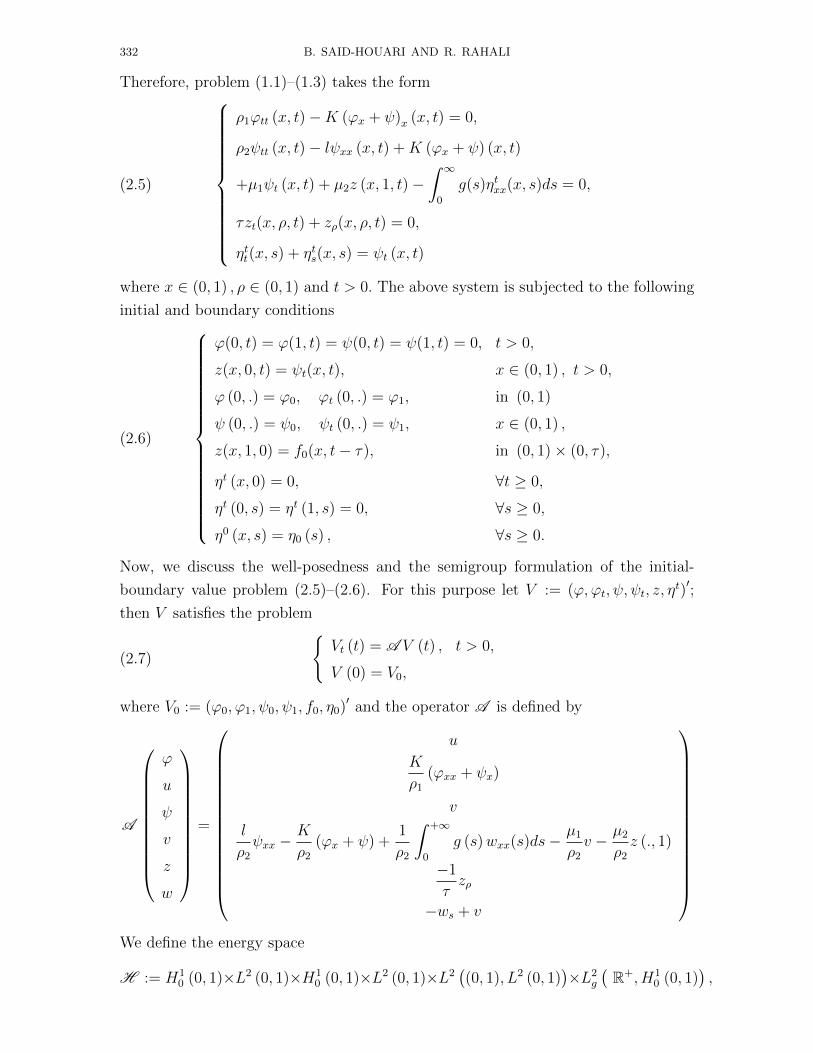
Therefore, problem (1.1)–(1.3) takes the form
(2.5)
ρ1ϕtt (x, t)−K (ϕx + ψ)x (x, t) = 0,
ρ2ψtt (x, t)− lψxx (x, t) +K (ϕx + ψ) (x, t)
+µ1ψt (x, t) + µ2z (x, 1, t)−∫ ∞
0
g(s)ηtxx(x, s)ds = 0,
τzt(x, ρ, t) + zρ(x, ρ, t) = 0,
ηtt(x, s) + ηts(x, s) = ψt (x, t)
where x ∈ (0, 1) , ρ ∈ (0, 1) and t > 0. The above system is subjected to the following
initial and boundary conditions
(2.6)
ϕ(0, t) = ϕ(1, t) = ψ(0, t) = ψ(1, t) = 0, t > 0,
z(x, 0, t) = ψt(x, t), x ∈ (0, 1) , t > 0,
ϕ (0, .) = ϕ0, ϕt (0, .) = ϕ1, in (0, 1)
ψ (0, .) = ψ0, ψt (0, .) = ψ1, x ∈ (0, 1) ,
z(x, 1, 0) = f0(x, t− τ), in (0, 1)× (0, τ),
ηt (x, 0) = 0, ∀t ≥ 0,
ηt (0, s) = ηt (1, s) = 0, ∀s ≥ 0,
η0 (x, s) = η0 (s) , ∀s ≥ 0.
Now, we discuss the well-posedness and the semigroup formulation of the initial-
boundary value problem (2.5)–(2.6). For this purpose let V := (ϕ, ϕt, ψ, ψt, z, ηt)′;
then V satisfies the problem
(2.7)
Vt (t) = A V (t) , t > 0,
V (0) = V0,
where V0 := (ϕ0, ϕ1, ψ0, ψ1, f0, η0)′ and the operator A is defined by
A
ϕ
u
ψ
v
z
w
=
u
K
ρ1
(ϕxx + ψx)
v
l
ρ2
ψxx −K
ρ2
(ϕx + ψ) +1
ρ2
∫ +∞
0
g (s)wxx(s)ds−µ1
ρ2
v − µ2
ρ2
z (., 1)
−1
τzρ
−ws + v
We define the energy space
H := H10 (0, 1)×L2 (0, 1)×H1
0 (0, 1)×L2 (0, 1)×L2((0, 1), L2 (0, 1)
)×L2
g
(R+, H1
0 (0, 1)),
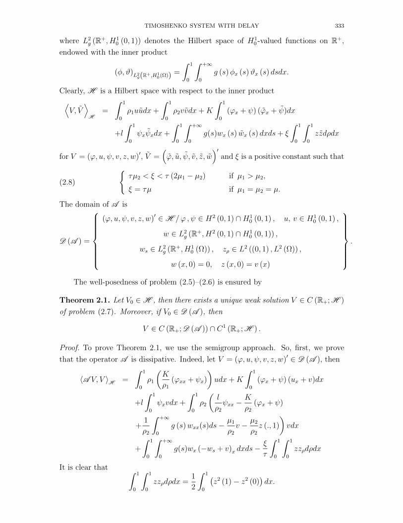
TIMOSHENKO SYSTEM WITH DELAY 333
where L2g (R+, H1
0 (0, 1)) denotes the Hilbert space of H10 -valued functions on R+,
endowed with the inner product
(φ, ϑ)L2g(R+,H1
0 (Ω)) =
∫ 1
0
∫ +∞
0
g (s)φx (s)ϑx (s) dsdx.
Clearly, H is a Hilbert space with respect to the inner product⟨V, V
⟩H
=
∫ 1
0
ρ1uudx+
∫ 1
0
ρ2vvdx+K
∫ 1
0
(ϕx + ψ) (ϕx + ψ)dx
+l
∫ 1
0
ψxψxdx+
∫ 1
0
∫ +∞
0
g(s)wx (s) wx (s) dxds+ ξ
∫ 1
0
∫ 1
0
zzdρdx
for V = (ϕ, u, ψ, v, z, w)′, V =(ϕ, u, ψ, v, z, w
)′and ξ is a positive constant such that
(2.8)
τµ2 < ξ < τ (2µ1 − µ2) if µ1 > µ2,
ξ = τµ if µ1 = µ2 = µ.
The domain of A is
D (A ) =
(ϕ, u, ψ, v, z, w)′ ∈H /ϕ , ψ ∈ H2 (0, 1) ∩H10 (0, 1) , u, v ∈ H1
0 (0, 1) ,
w ∈ L2g (R+, H2 (0, 1) ∩H1
0 (0, 1)) ,
ws ∈ L2g (R+, H1
0 (Ω)) , zρ ∈ L2 ((0, 1) , L2 (Ω)) ,
w (x, 0) = 0, z (x, 0) = v (x)
.
The well-posedness of problem (2.5)–(2.6) is ensured by
Theorem 2.1. Let V0 ∈H , then there exists a unique weak solution V ∈ C (R+; H )
of problem (2.7). Moreover, if V0 ∈ D (A ), then
V ∈ C (R+; D (A )) ∩ C1 (R+; H ) .
Proof. To prove Theorem 2.1, we use the semigroup approach. So, first, we prove
that the operator A is dissipative. Indeed, let V = (ϕ, u, ψ, v, z, w)′ ∈ D (A ), then
〈A V, V 〉H =
∫ 1
0
ρ1
(K
ρ1
(ϕxx + ψx)
)udx+K
∫ 1
0
(ϕx + ψ) (ux + v)dx
+l
∫ 1
0
ψxvdx+
∫ 1
0
ρ2
(l
ρ2
ψxx −K
ρ2
(ϕx + ψ)
+1
ρ2
∫ +∞
0
g (s)wxx(s)ds−µ1
ρ2
v − µ2
ρ2
z (., 1)
)vdx
+
∫ 1
0
∫ +∞
0
g(s)wx (−ws + v)x dxds−ξ
τ
∫ 1
0
∫ 1
0
zzρdρdx
It is clear that ∫ 1
0
∫ 1
0
zzρdρdx =1
2
∫ 1
0
(z2 (1)− z2 (0)
)dx.
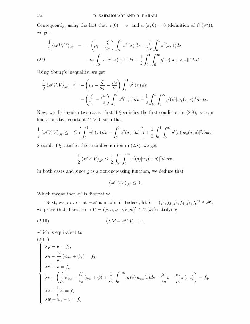
334 B. SAID-HOUARI AND R. RAHALI
Consequently, using the fact that z (0) = v and w (x, 0) = 0 (definition of D (A )),
we get
1
2〈A V, V 〉H = −
(µ1 −
ξ
2τ
)∫ 1
0
v2 (x) dx− ξ
2τ
∫ 1
0
z2(x, 1)dx
−µ2
∫ 1
0
v (x) z (x, 1) dx+1
2
∫ 1
0
∫ ∞0
g′(s)|wx(x, s)|2dsdx.(2.9)
Using Young’s inequality, we get
1
2〈A V, V 〉H ≤ −
(µ1 −
ξ
2τ− µ2
2
)∫ 1
0
v2 (x) dx
−(ξ
2τ− µ2
2
)∫ 1
0
z2(x, 1)dx+1
2
∫ 1
0
∫ ∞0
g′(s)|wx(x, s)|2dsdx.
Now, we distinguish two cases: first if ξ satisfies the first condition in (2.8), we can
find a positive constant C > 0, such that
1
2〈A V, V 〉H ≤ −C
∫ 1
0
v2 (x) dx+
∫ 1
0
z2(x, 1)dx
+
1
2
∫ 1
0
∫ ∞0
g′(s)|wx(x, s)|2dsdx.
Second, if ξ satisfies the second condition in (2.8), we get
1
2〈A V, V 〉H ≤
1
2
∫ 1
0
∫ ∞0
g′(s)|wx(x, s)|2dsdx.
In both cases and since g is a non-increasing function, we deduce that
〈A V, V 〉H ≤ 0.
Which means that A is dissipative.
Next, we prove that −A is maximal. Indeed, let F = (f1, f2, f3, f4, f5, f6)′ ∈H ,
we prove that there exists V = (ϕ, u, ψ, v, z, w)′ ∈ D (A ) satisfying
(2.10) (λId−A )V = F,
which is equivalent to
(2.11)
λϕ− u = f1,
λu− K
ρ1
(ϕxx + ψx) = f2,
λψ − v = f3,
λv −(l
ρ2
ψxx −K
ρ2
(ϕx + ψ) +1
ρ2
∫ +∞
0
g (s)wxx(s)ds−µ1
ρ2
v − µ2
ρ2
z (., 1)
)= f4.
λz +1
τzρ = f5
λw + ws − v = f6
TIMOSHENKO SYSTEM WITH DELAY 335
Suppose that we have found ϕ and ψ with the appropriate regularity. Therefore, the
first and the third equations in (2.11) give
(2.12)
u = λϕ− f1,
v = λψ − f3.
It is clear that u ∈ H10 (0, 1) and v ∈ H1
0 (0, 1). Furthermore, by using the fifth
equation in (2.11) we can find z with
(2.13) z (x, 0) = v (x) , for x ∈ (0, 1) .
Following the same approach as in [23] (see also [17]), we obtain, by using the fifth
equation in (2.11),
z (x, ρ) = v (x) e−λρτ + τe−λρτ∫ ρ
0
f5 (x, σ) eλστdσ.
From (2.12), we obtain
(2.14) z (x, ρ) = λψ (x) e−λρτ − f3e−λρτ + τe−λρτ
∫ ρ
0
f5 (x, σ) eλστdσ.
We note that the last equation in (2.11) with w (x, 0) = 0 has a unique solution
w (x, s) =
(∫ s
0
eλy (f6 (x, y) + v (x)) dy
)e−λs
=
(∫ s
0
eλy (f6 (x, y) + λψ (x)− f3 (x)) dy
)e−λs.(2.15)
By using (2.11), (2.12) and (2.15) the functions ϕ and ψ satisfy the following system
(2.16)
λ2ϕ− K
ρ1
(ϕxx + ψx) = f2 + λf1,(λ2 +
µ1λ
ρ2
+µ2λ
ρ2
e−λτ)ψ − lψxx +
K
ρ2
(ϕx + ψ) = f
where
l =l
ρ2
+λ
ρ2
∫ ∞0
g (s) e−λs(∫ s
0
eλydy
)ds
and
f = − 1
ρ2
∫ ∞0
g (s) e−λs(∫ s
0
eλy (f6 (x, y)− f3 (x))xx dy
)ds−
(λ+
µ1
ρ2
+µ2
ρ2
e−λτ)f3
+µ2τ
ρ2
e−λτ∫ 1
0
f5 (x, σ) eλστdτ.
We have just to prove that (2.16) has a solution (ϕ, ψ) ∈ (H2 (0, 1) ∩H10 (0, 1))
2and
replace in (2.12), (2.14) and (2.15) to get V = (ϕ, u, ψ, v, z, w)′ ∈ D (A ) satisfying
(2.10). Consequently, problem (2.16) is equivalent to the problem
(2.17) ζ ((ϕ, ψ) , (w, χ)) = l (w, χ)
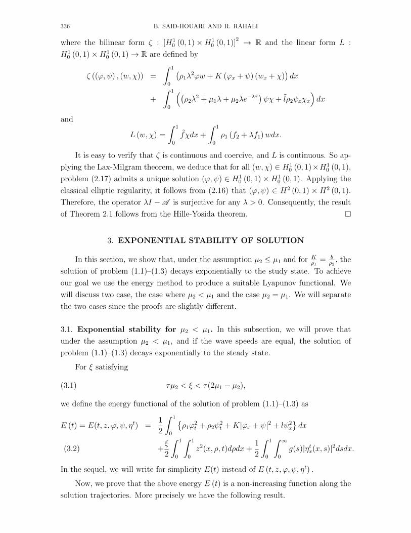
336 B. SAID-HOUARI AND R. RAHALI
where the bilinear form ζ : [H10 (0, 1)×H1
0 (0, 1)]2 → R and the linear form L :
H10 (0, 1)×H1
0 (0, 1)→ R are defined by
ζ ((ϕ, ψ) , (w, χ)) =
∫ 1
0
(ρ1λ
2ϕw +K (ϕx + ψ) (wx + χ))dx
+
∫ 1
0
((ρ2λ
2 + µ1λ+ µ2λe−λτ)ψχ+ lρ2ψxχx
)dx
and
L (w, χ) =
∫ 1
0
fχdx+
∫ 1
0
ρ1 (f2 + λf1)wdx.
It is easy to verify that ζ is continuous and coercive, and L is continuous. So ap-
plying the Lax-Milgram theorem, we deduce that for all (w, χ) ∈ H10 (0, 1)×H1
0 (0, 1),
problem (2.17) admits a unique solution (ϕ, ψ) ∈ H10 (0, 1)×H1
0 (0, 1). Applying the
classical elliptic regularity, it follows from (2.16) that (ϕ, ψ) ∈ H2 (0, 1) × H2 (0, 1).
Therefore, the operator λI −A is surjective for any λ > 0. Consequently, the result
of Theorem 2.1 follows from the Hille-Yosida theorem.
3. EXPONENTIAL STABILITY OF SOLUTION
In this section, we show that, under the assumption µ2 ≤ µ1 and for Kρ1
= bρ2
, the
solution of problem (1.1)–(1.3) decays exponentially to the study state. To achieve
our goal we use the energy method to produce a suitable Lyapunov functional. We
will discuss two case, the case where µ2 < µ1 and the case µ2 = µ1. We will separate
the two cases since the proofs are slightly different.
3.1. Exponential stability for µ2 < µ1. In this subsection, we will prove that
under the assumption µ2 < µ1, and if the wave speeds are equal, the solution of
problem (1.1)–(1.3) decays exponentially to the steady state.
For ξ satisfying
(3.1) τµ2 < ξ < τ(2µ1 − µ2),
we define the energy functional of the solution of problem (1.1)–(1.3) as
E (t) = E(t, z, ϕ, ψ, ηt) =1
2
∫ 1
0
ρ1ϕ
2t + ρ2ψ
2t +K|ϕx + ψ|2 + lψ2
x
dx
+ξ
2
∫ 1
0
∫ 1
0
z2(x, ρ, t)dρdx+1
2
∫ 1
0
∫ ∞0
g(s)|ηtx(x, s)|2dsdx.(3.2)
In the sequel, we will write for simplicity E(t) instead of E (t, z, ϕ, ψ, ηt) .
Now, we prove that the above energy E (t) is a non-increasing function along the
solution trajectories. More precisely we have the following result.
TIMOSHENKO SYSTEM WITH DELAY 337
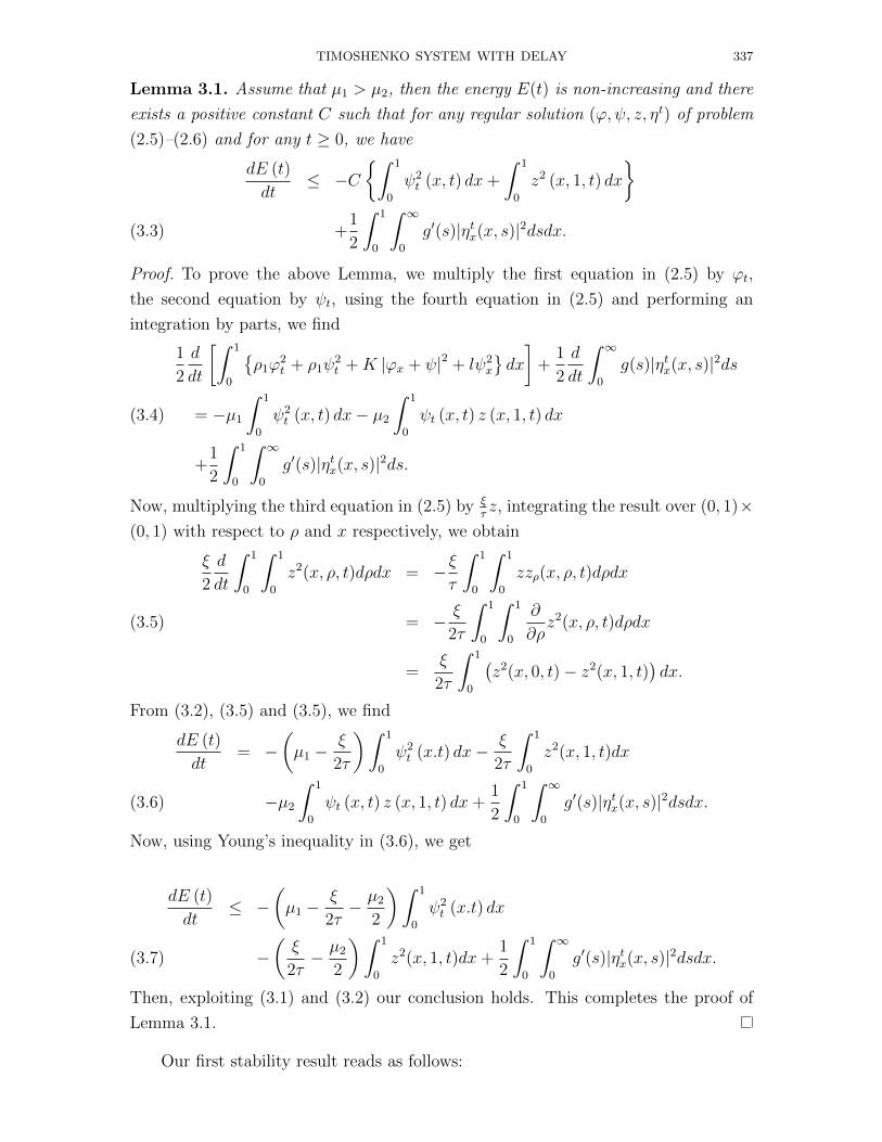
Lemma 3.1. Assume that µ1 > µ2, then the energy E(t) is non-increasing and there
exists a positive constant C such that for any regular solution (ϕ, ψ, z, ηt) of problem
(2.5)–(2.6) and for any t ≥ 0, we have
dE (t)
dt≤ −C
∫ 1
0
ψ2t (x, t) dx+
∫ 1
0
z2 (x, 1, t) dx
+
1
2
∫ 1
0
∫ ∞0
g′(s)|ηtx(x, s)|2dsdx.(3.3)
Proof. To prove the above Lemma, we multiply the first equation in (2.5) by ϕt,
the second equation by ψt, using the fourth equation in (2.5) and performing an
integration by parts, we find
1
2
d
dt
[∫ 1
0
ρ1ϕ
2t + ρ1ψ
2t +K |ϕx + ψ|2 + lψ2
x
dx
]+
1
2
d
dt
∫ ∞0
g(s)|ηtx(x, s)|2ds
= −µ1
∫ 1
0
ψ2t (x, t) dx− µ2
∫ 1
0
ψt (x, t) z (x, 1, t) dx(3.4)
+1
2
∫ 1
0
∫ ∞0
g′(s)|ηtx(x, s)|2ds.
Now, multiplying the third equation in (2.5) by ξτz, integrating the result over (0, 1)×
(0, 1) with respect to ρ and x respectively, we obtain
ξ
2
d
dt
∫ 1
0
∫ 1
0
z2(x, ρ, t)dρdx = − ξτ
∫ 1
0
∫ 1
0
zzρ(x, ρ, t)dρdx
= − ξ
2τ
∫ 1
0
∫ 1
0
∂
∂ρz2(x, ρ, t)dρdx(3.5)
=ξ
2τ
∫ 1
0
(z2(x, 0, t)− z2(x, 1, t)
)dx.
From (3.2), (3.5) and (3.5), we find
dE (t)
dt= −
(µ1 −
ξ
2τ
)∫ 1
0
ψ2t (x.t) dx− ξ
2τ
∫ 1
0
z2(x, 1, t)dx
−µ2
∫ 1
0
ψt (x, t) z (x, 1, t) dx+1
2
∫ 1
0
∫ ∞0
g′(s)|ηtx(x, s)|2dsdx.(3.6)
Now, using Young’s inequality in (3.6), we get
dE (t)
dt≤ −
(µ1 −
ξ
2τ− µ2
2
)∫ 1
0
ψ2t (x.t) dx
−(ξ
2τ− µ2
2
)∫ 1
0
z2(x, 1, t)dx+1
2
∫ 1
0
∫ ∞0
g′(s)|ηtx(x, s)|2dsdx.(3.7)
Then, exploiting (3.1) and (3.2) our conclusion holds. This completes the proof of
Lemma 3.1.
Our first stability result reads as follows:
338 B. SAID-HOUARI AND R. RAHALI
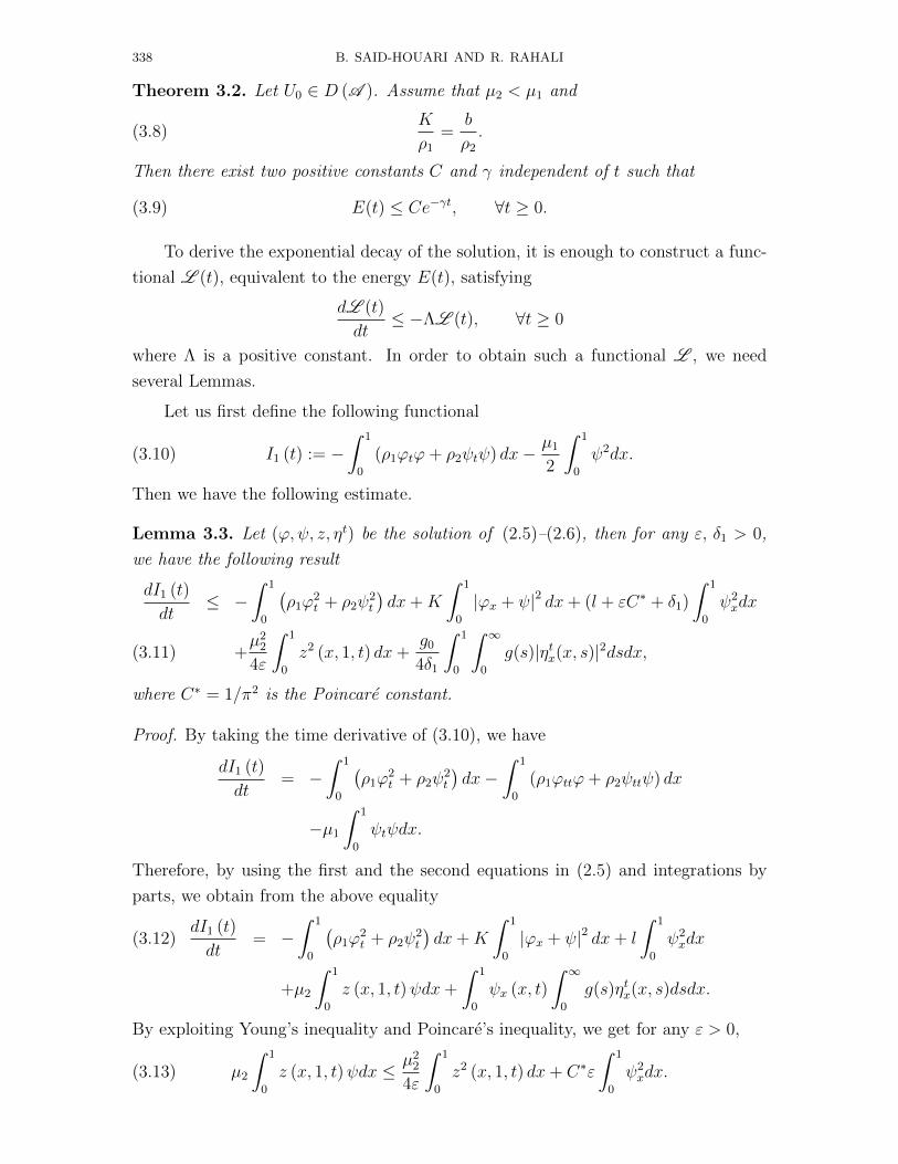
Theorem 3.2. Let U0 ∈ D (A ). Assume that µ2 < µ1 and
(3.8)K
ρ1
=b
ρ2
.
Then there exist two positive constants C and γ independent of t such that
(3.9) E(t) ≤ Ce−γt, ∀t ≥ 0.
To derive the exponential decay of the solution, it is enough to construct a func-
tional L (t), equivalent to the energy E(t), satisfying
dL (t)
dt≤ −ΛL (t), ∀t ≥ 0
where Λ is a positive constant. In order to obtain such a functional L , we need
several Lemmas.
Let us first define the following functional
(3.10) I1 (t) := −∫ 1
0
(ρ1ϕtϕ+ ρ2ψtψ) dx− µ1
2
∫ 1
0
ψ2dx.
Then we have the following estimate.
Lemma 3.3. Let (ϕ, ψ, z, ηt) be the solution of (2.5)–(2.6), then for any ε, δ1 > 0,
we have the following result
dI1 (t)
dt≤ −
∫ 1
0
(ρ1ϕ
2t + ρ2ψ
2t
)dx+K
∫ 1
0
|ϕx + ψ|2 dx+ (l + εC∗ + δ1)
∫ 1
0
ψ2xdx
+µ2
2
4ε
∫ 1
0
z2 (x, 1, t) dx+g0
4δ1
∫ 1
0
∫ ∞0
g(s)|ηtx(x, s)|2dsdx,(3.11)
where C∗ = 1/π2 is the Poincare constant.
Proof. By taking the time derivative of (3.10), we have
dI1 (t)
dt= −
∫ 1
0
(ρ1ϕ
2t + ρ2ψ
2t
)dx−
∫ 1
0
(ρ1ϕttϕ+ ρ2ψttψ) dx
−µ1
∫ 1
0
ψtψdx.
Therefore, by using the first and the second equations in (2.5) and integrations by
parts, we obtain from the above equality
dI1 (t)
dt= −
∫ 1
0
(ρ1ϕ
2t + ρ2ψ
2t
)dx+K
∫ 1
0
|ϕx + ψ|2 dx+ l
∫ 1
0
ψ2xdx(3.12)
+µ2
∫ 1
0
z (x, 1, t)ψdx+
∫ 1
0
ψx (x, t)
∫ ∞0
g(s)ηtx(x, s)dsdx.
By exploiting Young’s inequality and Poincare’s inequality, we get for any ε > 0,
(3.13) µ2
∫ 1
0
z (x, 1, t)ψdx ≤ µ22
4ε
∫ 1
0
z2 (x, 1, t) dx+ C∗ε
∫ 1
0
ψ2xdx.
TIMOSHENKO SYSTEM WITH DELAY 339
Moreover, Young’s inequality, Holder’s inequality and (G2) imply that for any δ1 > 0,
(3.14)∫ 1
0
ψx (x, t)
∫ ∞0
g(s)ηtx(x, s)dsdx ≤ δ1
∫ 1
0
ψ2x (x, t) dx+
g0
4δ1
∫ 1
0
∫ ∞0
g(s)|ηtx(x, s)|2dsdx.
Inserting the estimates (3.13) and (3.14) into (3.12), then (3.11) is fulfilled. Thus the
proof of Lemma 3.3 is finished.
Now, Let w be the solution of
(3.15) −wxx = ψx, w (0) = w (1) = 0.
Then, we have the following inequalities.
Lemma 3.4. The solution of (3.15) satisfies∫ 1
0
w2xdx ≤
∫ 1
0
ψ2dx
and ∫ 1
0
w2t dx ≤
∫ 1
0
ψ2t dx
Proof. We multiply Equation (3.15) by w, integrate by parts and use the Cauchy-
Schwarz inequality to obtain ∫ 1
0
w2xdx ≤
∫ 1
0
ψ2dx
Next, we differentiate (3.15) with respect to t and by the same procedure, we obtain∫ 1
0
w2t dx ≤
∫ 1
0
ψ2t dx
This completes the proof of Lemma 3.4.
Remark 3.5. The solution of (3.15) can be given explicitly as
w (x, t) = −∫ x
0
ψ (y, t) dy + x
(∫ 1
0
ψ (y, t) dy
).
Next, we introduce the following functional
(3.16) I2 :=
∫ 1
0
(ρ2ψtψ + ρ1ϕtω) dx+µ1
2
∫ 1
0
ψ2dx,
where w is the solution of (3.15). Then we have the following estimate.
Lemma 3.6. Let (ϕ, ψ, z, ηt) be the solution of (2.5)–(2.6), then for any δ1, λ2, λ2 >
0, we have
dI2 (t)
dt≤ (δ1 + µ2C
∗λ2 − l)∫ 1
0
ψ2x (x, t) dx+
(ρ2 +
ρ1
4λ2
)∫ 1
0
ψ2t (x, t) dx
+ρ1λ2
∫ 1
0
ϕ2t (x, t) dx+
µ2
4λ2
∫ 1
0
z2 (x, 1, t) dx(3.17)
340 B. SAID-HOUARI AND R. RAHALI
+g0
4δ1
∫ 1
0
∫ ∞0
g(s)|ηtx(x, s)|2dsdx.
Proof. By taking the derivative of (3.16) with respect to t and using the equations in
(2.5), we conclude
dI2 (t)
dt= −l
∫ 1
0
ψ2xdx+ ρ2
∫ 1
0
ψ2t dx−K
∫ 1
0
ψ2dx+K
∫ 1
0
ω2xdx
+ρ1
∫ 1
0
ϕtωtdx− µ2
∫ 1
0
ψz(x, 1, t) +
∫ 1
0
ψx(x, t)
∫ ∞0
g(s)ηtx(x, s)dsdx.
Using the first inequality in Lemma 3.4, we get
dI2 (t)
dt≤ −l
∫ 1
0
ψ2xdx+ ρ2
∫ 1
0
ψ2t dx+ ρ1
∫ 1
0
ϕtωtdx
−µ2
∫ 1
0
ψz(x, 1, t) +
∫ 1
0
ψx(x, t)
∫ ∞0
g(s)ηtx(x, s)dsdx.(3.18)
By using Young’s inequality and the second inequality in Lemma 3.4, we have for any
λ2 > 0
(3.19) ρ1
∫ 1
0
ϕtωtdx ≤ ρ1λ2
∫ 1
0
ϕ2t (x, t) dx+
ρ1
4λ2
∫ 1
0
ψ2t (x, t) dx.
Similarly, Young’s inequality and Poincare’s inequality give us the estimate
(3.20)
∣∣∣∣µ2
∫ 1
0
ψz (x, 1, t) dx
∣∣∣∣ ≤ µ2C∗λ2
∫ 1
0
ψ2xdx+
µ2
4λ2
∫ 1
0
z2 (x, 1, t) dx, ∀λ2 > 0.
Now, using the estimate (3.14) and inserting (3.19) and (3.20) into (3.18), then (3.17)
holds. Thus the proof of Lemma 3.6 is finished.
Next, we introduce the functional
J (t) : = ρ2
∫ 1
0
ψt (ϕx + ψ) dx+ρ1l
K
∫ 1
0
ψxϕtdx
+ρ1
K
∫ 1
0
ϕt
∫ ∞0
g(s)ηtx(x, s)dsdx.(3.21)
Then we have the following result.
Lemma 3.7. Let (ϕ, ψ, z, ηt) be the solution of (2.5)–(2.6). Assume that
(3.22)ρ1
K=
ρ2
l + g0
=ρ2
b.
Then, for any ε1 > 0, we conclude
dJ (t)
dt≤
[ϕx
(lψx +
∫ ∞0
g(s)ηtx(x, s)
)]x=1
x=0
− (K − 2ε)
∫ 1
0
(ϕx + ψ)2 dx
+
(ρ2 +
µ21
4ε1
)∫ 1
0
ψ2t dx+ ε1
∫ 1
0
ϕ2tdx+
µ22
4ε1
∫ 1
0
z2 (x, 1, t) dx(3.23)
−g0C(ε1)
∫ 1
0
∫ ∞0
g′(s)∣∣ηtx(x, s)∣∣2 dsdx.
TIMOSHENKO SYSTEM WITH DELAY 341
Proof. Differentiating J (t), with respect to t, we obtain
dJ (t)
dt= ρ2
∫ 1
0
ψtt (ϕx + ψ) dx+ ρ2
∫ 1
0
ψt (ϕx + ψ)t dx
+ρ1l
K
∫ 1
0
ψxϕttdx+ρ1
K
∫ 1
0
ϕt
∫ ∞0
g(s)ηttx(x, s)dsdx
+ρ1l
K
∫ 1
0
ψtxϕtdx+ρ1
K
∫ 1
0
ϕtt
∫ ∞0
g(s)ηtx(x, s)dsdx.
Then, by using equations in (2.5), we find
dJ (t)
dt=
∫ 1
0
(ϕx + ψ) [lψxx (x, t)−K (ϕx + ψ) (x, t)− µ1ψt (x, t)− µ2z (x, 1, t)] dx
+
∫ 1
0
(ϕx + ψ)
∫ ∞0
g(s)ηtxx(x, s)dsdx+ ρ2
∫ 1
0
ψ2t dx+ l
∫ 1
0
(ϕx + ψ)x ψxdx
+
(ρ1l
K− ρ2
)∫ 1
0
ψtxϕtdx+ρ1
K
∫ 1
0
ϕt
∫ ∞0
g(s)(ψtx (t, x)− ηtsx(x, s))dsdx
+
∫ 1
0
(ϕx + ψ)x
∫ ∞0
g(s)ηtx(x, s)dsdx.
Using (3.22), we obtain
dJ (t)
dt= −K
∫ 1
0
(ϕx + ψ)2 − µ1
∫ 1
0
(ϕx + ψ)ψtdx+ ρ2
∫ 1
0
ψ2t dx
−µ2
∫ 1
0
(ϕx + ψ) z (x, 1, t) dx+ρ1
K
∫ 1
0
ϕt
∫ ∞0
g′(s)ηtx(x, s)dsdx(3.24)
+ [lϕxψx]x=1x=0 +
[ϕx (x, t)
∫ ∞0
g(s)ηtx(x, s)ds
]x=1
x=0
.
For any ε1 > 0, Young’s inequality leads to
(3.25)
∣∣∣∣µ1
∫ 1
0
(ϕx + ψ)ψtdx
∣∣∣∣ ≤ ε1
∫ 1
0
(ϕx + ψ)2 dx+µ2
1
4ε1
∫ 1
0
ψ2t dx,
(3.26)
∣∣∣∣µ2
∫ 1
0
(ϕx + ψ) z (x, 1, t) dx
∣∣∣∣ ≤ ε1
∫ 1
0
(ϕx + ψ)2 dx+µ2
2
4ε1
∫ 1
0
z2 (x, 1, t) dx,
and ∣∣∣∣ρ1
K
∫ 1
0
ϕt
∫ ∞0
g′(s)ηtx(x, s)dsdx
∣∣∣∣≤ ρ2
1
4K2ε1
∫ 1
0
(∫ ∞0
g′(s)ηtx(x, s)ds
)2
dx+ ε1
∫ 1
0
ϕ2tdx(3.27)
≤ −g (0)C (ε1)
∫ 1
0
∫ ∞0
g′(s)∣∣ηtx(x, s)∣∣2 dsdx+ ε1
∫ 1
0
ϕ2tdx.
Plugging (3.25), (3.26) and (3.27) into (3.24), then inequality (3.23) holds.
342 B. SAID-HOUARI AND R. RAHALI
Next, in order to handle the boundary terms, appearing in (3.23), we use the
function
q (x) = 2− 4x, x ∈ (0, 1) .
So, we have the following result.
Lemma 3.8. Let (ϕ, ψ, z, ηt) be the solution of (2.5)–(2.6). Then for any ε2 > 0,
the following estimate holds[ϕx
(lψx +
∫ ∞0
g(s)ηtx(x, s)ds
)]x=1
x=0
(3.28)
≤ −ε2
K
d
dt
∫ 1
0
ρ1q (x)ϕtϕxdx+K2ε2
∫ 1
0
(ϕx + ψ)2 dx
− 1
4ε2
d
dt
∫ 1
0
ρ2q (x)ψt
(lψx +
∫ ∞0
g(s)ηtx(x, s)ds
)dx+ 3ε2
∫ 1
0
ϕ2xdx
+
(ε2 +
l2
4ε2
(4 +
3
2ε22
))∫ 1
0
ψ2xdx+
1
4ε2
(2ρ2(l + g0) + 4µ2
1ε22 + ρ2ε2
) ∫ 1
0
ψ2t dx
−ρ2g(0)C(ε2)
4ε2
∫ 1
0
∫ ∞0
g′(s)∣∣ηtx(x, s)∣∣2 dsdx+
2ρ1ε2
K
∫ 1
0
ϕ2tdx
+g0
4ε2
(4 +
3
2ε22
)∫ 1
0
∫ ∞0
g(s)∣∣ηtx(x, s)∣∣2 dsdx+ µ2
2ε2
∫ 1
0
z2 (x, 1, t) dx.
Proof. By using Young’s inequality, we easily see that, for any ε2 > 0,[ϕx
(lψx +
∫ ∞0
g(s)ηtx(x, s)
)]x=1
x=0
≤ ε2
[ϕ2x(1, t) + ϕ2
x(0, t)]
+1
4ε2
(lψx (0, t) +
∫ ∞0
g(s)ηtx(0, s)ds
)2
(3.29)
+1
4ε2
(lψx (1, t) +
∫ ∞0
g(s)ηtx(1, s)ds
)2
.
On the other hand, it is clear that
d
dt
∫ 1
0
ρ2q (x)ψt
(lψx +
∫ ∞0
g(s)ηtx(x, s)ds
)dx
=
∫ 1
0
ρ2q (x)ψtt
(lψx +
∫ ∞0
g(s)ηtx(x, s)ds
)dx
+
∫ 1
0
ρ2q (x)ψt
(lψxt +
∫ ∞0
g(s)ηtxt(x, s)ds
)dx.(3.30)
Now, using the second equation in (2.5), we find
d
dt
∫ 1
0
ρ2q (x)ψt
(lψx +
∫ ∞0
g(s)ηtx(x, s)ds
)dx
=
∫ 1
0
q(x)(lψxx (x, t)−K (ϕx + ψ) (x, t)
TIMOSHENKO SYSTEM WITH DELAY 343
− µ1ψt (x, t)− µ2z (x, 1, t) +
∫ ∞0
g(s)ηtxx(x, s)ds)
×(lψx +
∫ ∞0
g(s)ηtx(x, s)ds
)dx
+
∫ 1
0
ρ2q (x)ψt
(lψxt +
∫ ∞0
g(s)ηtxt(x, s)ds
)dx.(3.31)
By noticing that∫ 1
0
q (x)
(lψxx (x, t) +
∫ ∞0
g(s)ηtxx(x, s)ds
)(lψx +
∫ ∞0
g(s)ηtx(x, s)ds
)dx
= −1
2
∫ 1
0
q′ (x)
(lψx (x, t) +
∫ ∞0
g(s)ηtx(x, s)ds
)2
dx
+
[q (x)
2
(lψx (x, t) +
∫ ∞0
g(s)ηtx(x, s)ds
)2]x=1
x=0
.(3.32)
The last term in (3.31) can be treated as follows:∫ 1
0
ρ2q (x)ψt
(lψxt +
∫ ∞0
g(s)ηtxt(x, s)ds
)dx(3.33)
= ρ2l
∫ 1
0
q (x)ψtψxtdx+ ρ2
∫ 1
0
q (x)ψt
∫ ∞0
g(s)ηtxt(x, s)dsdx
= −ρ2l
2
∫ 1
0
q′ (x)ψ2t dx+ ρ2
∫ 1
0
q (x)ψt
∫ ∞0
g(s)ηtxt(x, s)dsdx
= −ρ2l
2
∫ 1
0
q′ (x)ψ2t dx+ ρ2
∫ 1
0
q (x)ψt
∫ ∞0
g(s)(ψt − ηts)xdsdx
= −ρ2l
2
∫ 1
0
q′ (x)ψ2t dx+ ρ2g0
∫ 1
0
q (x)ψtψtxdx− ρ2
∫ 1
0
q (x)ψt
∫ ∞0
g(s)ηtsxdsdx
= −ρ2(l + g0)
2
∫ 1
0
q′ (x)ψ2t dx+ ρ2
∫ 1
0
q (x)ψt
∫ ∞0
g′(s)ηtxdsdx
Inserting (3.32) and (3.34) in (3.31), we arrive at(lψx(0, t) +
∫ ∞0
g(s)ηtx(0, s)ds
)2
+
(lψx(1, t) +
∫ ∞0
g(s)ηtx(1, s)ds
)2
= − d
dt
∫ 1
0
ρ2qψt
(lψx +
∫ ∞0
g(s)ηtx(x, s)ds
)dx+ 2ρ2(l + g0)
∫ 1
0
ψ2t dx
−K∫ 1
0
q (ϕx + ψ)
(lψx +
∫ ∞0
g(s)ηtx(x, s)ds
)dx
+ρ2
∫ 1
0
qψt
∫ ∞0
g′(s)ηtxdsdx− µ1
∫ 1
0
q (x)ψt
(lψx +
∫ ∞0
g(s)ηtx(x, s)ds
)dx(3.34)
+2
∫ 1
0
(lψx +
∫ ∞0
g(s)ηtx(x, s)ds
)2
dx
344 B. SAID-HOUARI AND R. RAHALI
−µ2
∫ 1
0
q (x) z (x, 1, t)
(lψx +
∫ ∞0
g(s)ηtx(x, s)ds
)dx.
Now, we estimate some terms in the right hand sides of (3.34) as follows:
First, using Minkowski and Young’s inequalities, we infer that
2
∫ 1
0
(lψx +
∫ ∞0
g(s)ηtx(x, s)ds
)2
dx
≤ 4l2∫ 1
0
ψ2xdx+ 4g0
∫ 1
0
∫ ∞0
g(s)∣∣ηtx(x, s)∣∣2 dsdx.(3.35)
Second, by Young’s inequality and (3.35) we have, for any λ > 0∣∣∣∣K ∫ 1
0
q (x) (ϕx + ψ)
(lψx +
∫ ∞0
g(s)ηtx(x, s)ds
)dx
∣∣∣∣≤ 2K
∣∣∣∣∫ 1
0
(ϕx + ψ)
(lψx +
∫ ∞0
g(s)ηtx(x, s)ds
)dx
∣∣∣∣≤ 4K2λ
∫ 1
0
(ϕx + ψ)2 dx+1
4λ
∫ 1
0
(lψx +
∫ ∞0
g(s)ηtx(x, s)ds
)2
dx
≤ 4K2λ
∫ 1
0
(ϕx + ψ)2 dx+l2
2λ
∫ 1
0
ψ2xdx+
g0
2λ
∫ 1
0
∫ ∞0
g(s)∣∣ηtx(x, s)∣∣2 dsdx.
Similarly, we get∣∣∣∣µ1
∫ 1
0
q (x)ψt
(lψx +
∫ ∞0
g(s)ηtx(x, s)ds
)dx
∣∣∣∣≤ 4µ2
1λ
∫ 1
0
ψ2t dx+
l2
2λ
∫ 1
0
ψ2xdx+
g0
2λ
∫ 1
0
∫ ∞0
g(s)∣∣ηtx(x, s)∣∣2 dsdx
and ∣∣∣∣µ2
∫ 1
0
q (x) z (x, 1, t)
(lψx +
∫ ∞0
g(s)ηtx(x, s)ds
)dx
∣∣∣∣≤ 4µ2
2λ
∫ 1
0
z2 (x, 1, t) dx+l2
2λ
∫ 1
0
ψ2xdx+
g0
2λ
∫ 1
0
∫ ∞0
g(s)∣∣ηtx(x, s)∣∣2 dsdx.
Also, it is clear that for any ε2 > 0, we have∣∣∣∣ρ2
∫ 1
0
qψt
∫ ∞0
g′(s)ηtsdsdx
∣∣∣∣≤ ρ2ε2
∫ 1
0
ψ2t dx− ρ2g(0)C(ε2)
∫ 1
0
∫ ∞0
g′(s)∣∣ηtx(x, s)∣∣2 dsdx.
Inserting all the above estimates into (3.34), we obtain(lψx(0, t) +
∫ ∞0
g(s)ηtx(0, s)ds
)2
+
(lψx(1, t) +
∫ ∞0
g(s)ηtx(1, s)ds
)2
≤ − d
dt
∫ 1
0
ρ2q (x)ψt
(lψx +
∫ ∞0
g(s)ηtx(x, s)ds
)dx
TIMOSHENKO SYSTEM WITH DELAY 345
+(2ρ2(l + g0) + 4µ2
1λ+ ρ2ε2
) ∫ 1
0
ψ2t dx
+l2(
4 +3
2λ
)∫ 1
0
ψ2xdx+ 4K2λ
∫ 1
0
(ϕx + ψ)2 dx(3.36)
−ρ2g(0)C(ε2)
∫ 1
0
∫ ∞0
g′(s)∣∣ηtx(x, s)∣∣2 dsdx
+g0
(4 +
3
2λ
)∫ 1
0
∫ ∞0
g(s)∣∣ηtx(x, s)∣∣2 dsdx+ 4µ2
2λ
∫ 1
0
z2 (x, 1, t) dx.
On the other hand, we have
(ϕ2x(1, t) + ϕ2
x(0, t))≤ − 1
K
d
dt
∫ 1
0
ρ1q (x)ϕtϕxdx+ 3
∫ 1
0
ϕ2xdx
+
∫ 1
0
ψ2xdx+
2ρ1
K
∫ 1
0
ϕ2tdx.(3.37)
Consequently, by plugging the estimates (3.37) and (3.37) into (3.29), then our desired
estimate (3.29) holds true. This completes the proof of Lemma 3.8.
Now, let us introduce the following functional (see [23])
(3.38) I3 (t) :=
∫ 1
0
∫ 1
0
e−2τρz2(x, ρ, t)dρdx.
Then the following result holds.
Lemma 3.9. Let (ϕ, ψ, z, ηt) be the solution of (2.5)–(2.6). Then we have
(3.39)d
dtI3 (t) ≤ −I3 (t)− c
2τ
∫ 1
0
z2(x, 1, t)dx+1
2τ
∫ 1
0
ψ2t (x, t)dx,
where c is a positive constant.
Proof. Differentiating (3.38) with respect to t and using the third equation in (2.5),
we have
d
dt
(∫ 1
0
∫ 1
0
e−2τρz2(x, ρ, t)dρdx
)= −1
τ
∫ 1
0
∫ 1
0
e−2τρzzρ(x, ρ, t)dρdx
= −∫ 1
0
∫ 1
0
e−2τρz2(x, ρ, t)dρdx− 1
2τ
∫ 1
0
∫ 1
0
∂
∂ρ
(e−2τρz2(x, ρ, t)
)dρdx.
By recalling (2.6), the above equality implies that there exists a positive constant c
such that (3.39) holds.
346 B. SAID-HOUARI AND R. RAHALI
Proof of Theorem 3.2. To finalize the proof of Theorem 3.2, we define the Lyapunov
functional L (t) as follows
L (t) : = ME (t) +1
4I1 (t) +N2I2 (t) + J (t) +
ε2
K
∫ 1
0
ρ1qϕtϕxdx
+1
4ε2
∫ 1
0
ρ2q (x)ψt
(lψx +
∫ ∞0
g(s)ηtx(x, s)ds
)dx+ I3 (t) ,(3.40)
where M, N1, N2 and ε2 are positive real numbers which will be chosen later. Con-
sequently, the estimates (3.3), (3.11), (3.17), (3.23), (3.29) and (3.39) together with
(1.4) and the following inequality
(3.41)
∫ 1
0
ϕ2xdx ≤ 2
∫ 1
0
(ϕx + ψ)2 dx+ 2
∫ 1
0
ψ2xdx
lead to
d
dtL (t) ≤
[−MC − ρ1
4+N2
(ρ2 +
ρ1
4λ2
)+
(ρ2 +
µ21
4ε1
)+
1
4ε2
(2ρ2(l + g0) + 4µ2
1ε22 + ρ2ε2
)+
1
2τ
] ∫ 1
0
ψ2t dx
+
[−MC +
µ22
16ε+N2µ2
4λ2
+µ2
2
4ε1
+ µ22ε2 −
c
2τ
] ∫ 1
0
z2(x, 1, t)dx
+
[−ρ1
4+N2ρ1λ2 +
2ρ1ε2
K+ ε1
] ∫ 1
0
ϕ2tdx
+
[−(
3K
4− 2ε
)+K2ε2 + 6ε2
] ∫ 1
0
(ϕx + ψ)2 dx− I3 (t)
+
[1
4(l + εC∗ + δ1) +N2 (δ1 + µ2C
∗λ2 − l)(3.42)
+
(7ε2 +
l2
4ε2
(4 +3
2ε22
)]∫ 1
0
ψ2xdx+
[g0
4δ1
(1
4+N2
)+
g0
4ε2
(4 +
3
2ε22
)−ζ(M
2− g0C(ε1)− ρ2g(0)C(ε2)
4ε2
)]∫ 1
0
∫ ∞0
g(s)∣∣ηtx(x, s)∣∣2 dsdx.
At this point, we have to choose our constants very carefully. First, let us choose ε
small enough such that
ε <3K
8.
Then, take ε1 = ε2 and choose ε2 small enough such that
ε2 ≤ min
(K/8
K2 + 6,
ρ1/8
(2ρ1/K) + 1
)After that, we select δ1 = λ2 and choose λ2 small enough such that
λ2 ≤l/2
1 + µ2C∗.
TIMOSHENKO SYSTEM WITH DELAY 347
Once all the above constants are fixed, we fix N2 large enough such that
N2l
4≥ 1
4(l + εC∗ + δ1) + 7ε2 +
l2
4ε2
(4 +
3
2ε22
).
After that, we pick λ2 so small that
λ2 ≤1
32N2
.
Finally, we choose M large enough so that, there exists a positive constant η1, such
that (3.42) becomes
d
dtL (t) ≤ −η1
∫ 1
0
(ψ2t + ψ2
x + ϕ2t + (ϕx + ψ)2 + z2(x, 1, t)
)dx
−η1
∫ 1
0
∫ 1
0
z2(x, ρ, t)dρdx− η1
∫ 1
0
∫ ∞0
g(s)∣∣ηtx(x, s)∣∣2 dsdx,(3.43)
which implies by (3.2), that there exists also η2 > 0, such that
(3.44)d
dtL (t) ≤ −η2E (t) , ∀t ≥ 0.
We also have the following lemma.
Lemma 3.10. For M large enough, there exist two positive constants β1 and β2
depending on M,N2 and ε2, such that
(3.45) β1E (t) ≤ L (t) ≤ β2E (t) , ∀t ≥ 0.
Next, combining (3.44) and (3.45), we conclude that there exists Λ > 0 such that
(3.46)d
dtL (t) ≤ −ΛL (t) , ∀t ≥ 0.
A simple integration of (3.46) leads to
(3.47) L (t) ≤ L (0) e−Λt, ∀t ≥ 0.
Again, use of (3.45) and (3.47) yields the desired result (3.9). This completes the
proof of Theorem 3.2.
3.2. Exponential stability for µ1 = µ2. In this subsection we assume that µ1 =
µ2 = µ. As we will see, we cannot directly perform the same proof as for the case
where µ2 < µ1. We point out here that in the absence of the viscoelastic damping,
that is for g = 0, Said-Houari and Laskri [23] have proved recently an exponential
stability result for µ1 > µ2. Here we push the result in [23] to the case where µ1 = µ2
and we show that the presence of the viscoelastic damping in the second equation in
(1.1) may extend the set of (µ1, µ2) for which the exponential stability of (1.1)–(1.3)
occurs. For the wave equation, Nicaise and Pignotti have proved recently in [17] that
for µ1 = µ2 some instabilities results hold.
Our main result in this section reads as follows.
348 B. SAID-HOUARI AND R. RAHALI
Theorem 3.11. Let U0 ∈ D (A ). Assume that µ2 = µ1 = µ and g satisfies (G1)
and (G2). Assume further that (3.8) holds. Then there exist two positive constants
C and γ such that for any solution (ϕ, ψ, z, ηt) of problem (2.5)–(2.6), we have
(3.48) E (t) ≤ Ce−γt, ∀t ≥ 0.
To prove Theorem 3.11, we need some additional Lemmas. First, if µ1 = µ2 = µ,
then we can choose ξ = τµ. In this case Lemma 3.1 takes the form
Lemma 3.12. Assume that µ2 = µ1 = µ, then the energy E(t) is non-increasing
and there exists a positive constant C such that for any regular solution (ϕ, ψ, z, ηt)
of problem (2.5)–(2.6) and for any t ≥ 0, we have
(3.49)dE (t)
dt≤ 1
2
∫ 1
0
∫ ∞0
g′(s)|ηtx(x, s)|2dsdx ≤ 0.
The proof of Lemma 3.12 is an immediate consequence of Lemma 3.1, by choosing
ξ = τµ.
If µ2 = µ1, we need some additional negative terms of∫ 1
0ψt(x, t)dx, for this
purpose, let us introduce the functional:
(3.50) I4 = −ρ2
∫ 1
0
ψt(x, t)
∫ ∞0
g(s)ηt(x, s)dsdx.
Then, we have the following estimate.
Lemma 3.13. Let (ϕ, ψ, z, ηt) be the solution of (2.5)–(2.6). Then we have
d
dtI4 (t) ≤
(µ2γ3 −
ρ2g0
2
)∫ 1
0
ψ2t (x, t)dx+ l2γ1
∫ 1
0
ψ2x(x, t)dx+K2γ2
∫ 1
0
(ϕx + ψ)2 dx
+
(g0 +
g0
4γ1
+g0C
∗
4γ2
+g0C
∗
4
(1
γ3
+1
γ4
))∫ 1
0
∫ ∞0
g(s)∣∣ηtx(x, s)∣∣2 dsdx(3.51)
−C∗ρ2g(0)
2
∫ 1
0
∫ ∞0
g′(s)∣∣ηtx(x, s)∣∣2 dsdx+ µ2γ4
∫ 1
0
z2 (x, 1, t) dx.
Proof. Differentiating (3.50) with respect to t, we get
dI4(t)
dt=
∫ 1
0
(−lψxx (x, t) +K (ϕx + ψ) (x, t)
+µψt (x, t) + µz (x, 1, t)−∫ ∞
0
g(s)ηtxx(x, s)ds
)×(∫ ∞
0
g(s)ηt(x, s)dsdx
)−ρ2
∫ 1
0
ψt(x, t)
∫ ∞0
g(s)ηtt(x, s)dsdx.(3.52)
The terms in the right hand side of (3.52) can be estimated as follows:
First, using integration by parts, the boundary conditions (2.6), Holder’s inequal-
ity and Young’s inequality, we get for any γ1 > 0
−∫ 1
0
lψxx (x, t)
∫ ∞0
g(s)ηt(x, s)dsdx
TIMOSHENKO SYSTEM WITH DELAY 349
=
∫ 1
0
lψx (x, t)
∫ ∞0
g(s)ηtx(x, s)dsdx
≤ l2γ1
∫ 1
0
ψ2x (x, t) dx+
1
4γ1
∫ 1
0
(∫ ∞0
g(s)ηtx(x, s)dsdx
)2
dx
≤ l2γ1
∫ 1
0
ψ2x (x, t) dx+
g0
4γ1
∫ 1
0
∫ ∞0
g(s)∣∣ηtx(x, s)∣∣2 dsdx.
Second, Poincare’s inequality and Young’s inequality give for any γ2 > 0∫ 1
0
K (ϕx + ψ) (x, t)
∫ ∞0
g(s)ηt(x, s)dsdx
≤ K2γ2
∫ 1
0
|ϕx + ψ|2 (x, t) dx+g0C
∗
4γ2
∫ 1
0
∫ ∞0
g(s)∣∣ηtx(x, s)∣∣2 dsdx.
Third, as above we have for all γ3, γ4 > 0∫ 1
0
(µψt (x, t) + µz (x, 1, t))
∫ ∞0
g(s)ηt(x, s)dsdx
≤ µ2
∫ 1
0
(γ3ψ
2t (x, t) + γ4z
2 (x, 1, t))dx+
g0C∗
4
(1
γ3
+1
γ4
)∫ 1
0
∫ ∞0
g(s)∣∣ηtx(x, s)∣∣2 dsdx.
Fourth, it is obvious that
−∫ 1
0
∫ ∞0
g(s)ηtxx(x, s)ds
∫ ∞0
g(s)ηt(x, s)dsdx
=
∫ 1
0
(∫ ∞0
g(s)ηtx(x, s)ds
)2
dx
≤ g0
∫ 1
0
∫ ∞0
g(s)∣∣ηtx(x, s)∣∣2 dsdx.
Fifth, we have
−ρ2
∫ 1
0
ψt(x, t)
∫ ∞0
g(s)ηtt(x, s)dsdx = −ρ2g0
∫ 1
0
ψ2t (x, t)dx
− ρ2
∫ 1
0
ψt(x, t)
∫ ∞0
g′(s)ηt(x, s)dsdx.
On the other hand, it is clear that∣∣∣∣ρ2
∫ 1
0
ψt(x, t)
∫ ∞0
g′(s)ηt(x, s)dsdx
∣∣∣∣ ≤ ρ2g0
2
∫ 1
0
ψ2t (x, t)dx
−C∗g (0) ρ2
2
∫ 1
0
∫ ∞0
g′(s)∣∣ηtx(x, s)∣∣2 dsdx.
This last inequality implies
−ρ2
∫ 1
0
ψt(x, t)
∫ ∞0
g(s)ηtt(x, s)dsdx ≤ −ρ2g0
2
∫ 1
0
ψ2t (x, t)dx
−C∗g (0) ρ2
2
∫ 1
0
∫ ∞0
g′(s)∣∣ηtx(x, s)∣∣2 dsdx.
350 B. SAID-HOUARI AND R. RAHALI
Inserting all the above estimates into (3.52), then our result (3.51) is obtained. This
completes the proof of Lemma 3.13.
To finalize the proof of Theorem 3.11, we define the Lyapunov functional F (t)
as follows
F (t) := NE (t) +1
4I1 (t) + N2I2 (t) + J (t) +
ε2
K
∫ 1
0
ρ1qϕtϕxdx
+1
4ε2
∫ 1
0
ρ2q (x)ψt
(lψx +
∫ ∞0
g(s)ηtx(x, s)ds
)dx+N3I3 (t) +N4I4 (t) ,(3.53)
where N, N1, N2, N3, N4 and ε2 are positive real numbers which will be chosen later.
Consequently, using the estimates (3.11), (3.17), (3.23), (3.29), (3.39), (3.49) and
(3.51) together with (1.4) and the algebraic inequality (3.41) we get
d
dtF (t) ≤
[−ρ2
4+ N2
(ρ2 +
ρ1
4λ2
)+
1
4ε2
(2ρ2(l + g0) + 4µ2
1ε22 + ρ2ε2
)+
(ρ2 +
µ21
4ε1
)+N3
2τ+N4
(µ2γ3 −
ρ2g0
2
)]∫ 1
0
ψ2t dx
+
[µ2
2
16ε+ N2
µ2
4λ2
+µ2
2
4ε1
+ µ22ε2 −
N3c
2τ+N4µ
2γ4
] ∫ 1
0
z2(x, 1, t)dx
+
[−ρ1
4+ ε1 +
2ρ1ε2
K+ N2ρ1λ2
] ∫ 1
0
ϕ2tdx−N3I3 (t)
+
[− (K − 2ε) +
K
4+K2ε2 +N4K
2γ2 + 6ε2
] ∫ 1
0
(ϕx + ψ)2 dx(3.54)
+
[1
4(l + εC∗ + δ1) + N2 (δ1 + µ2C
∗λ2 − l)
+l2
4ε2
(4 +
3
2ε22
)+N4l
2γ1 + 7ε2
] ∫ 1
0
ψ2xdx
+ C
∫ 1
0
∫ ∞0
g(s)∣∣ηtx(x, s)∣∣2 dsdx.
where
C =g0
16δ1
+ N2g0
4δ1
+g0
4ε2
(4 +
3
2ε22
)+N4
(g0 +
g0
4γ1
+g0C
∗
4γ2
+g0C
∗
4
(1
γ3
+1
γ4
))−ζ(N
2− g0C(ε1)− ρ2g(0)C(ε2)
4ε2
− N4C∗ρ2g(0)
2
).
Now, our goal is to choose our constant in (3.54) in order to get negative coefficients
on the the right-hand side of (3.54). To this end, let us first choose ε small enough
such that
ε ≤ K
4.
TIMOSHENKO SYSTEM WITH DELAY 351
Then, take ε1 = ε2 and choose ε2 small enough such that
ε2 ≤ min
(K/8
K2 + 6,
ρ1/8
(2ρ1/K) + 1
).
Also, we pick γ3 sufficiently small such that
γ3 ≤ρ2g0
4µ2.
Next, we select δ1 = λ2 and choose λ2 small enough such that
λ2 ≤l/2
1 + µ2C∗.
Once all the above constants are fixed, we fix N2 large enough such that
N2l
4≥ 1
4(l + εC∗ + δ1) + 7ε2 +
l2
4ε2
(4 +
3
2ε22
)After that, we pick λ2 so small that
λ2 ≤1
32N2
.
Furthermore, choosing N3 large enough such that
N3c
4τ≥ µ2
2
16ε+ N2
µ2
4λ2
+µ2
2
4ε1
+ µ22ε2.
Next, we fix N4 large enough such that
N4ρ2g0
2≥(ρ2 +
µ21
4ε1
)+N3
2τ+ N2
(ρ2 +
ρ1
4λ2
)+
1
4ε2
(2ρ2(l + g0) + 4µ2
1ε22 + ρ2ε2
).
Once N4 and all the above constants are fixed, we may choose γ1, γ2 and γ4 small
enough such that
γ2 ≤1
16KN4
, γ1 ≤N2
8N4l, γ4 ≤
N3c
8τN4µ2.
Once all the above constants are fixed, we pick N large enough such that there exists
η1 such that
d
dtF (t) ≤ −η1
∫ 1
0
(ψ2t + ψ2
x + ϕ2t + (ϕx + ψ)2 + z2(x, 1, t)
)dx
−η1
∫ 1
0
∫ 1
0
z2(x, ρ, t)dρdx− η1
∫ 1
0
∫ ∞0
g(s)∣∣ηtx(x, s)∣∣2 dsdx.(3.55)
On the other hand, for N large enough,we can find two positive constants β1 and β2
depending on N, N2, N3, N4 and ε2 such that
(3.56) β1E (t) ≤ F (t) ≤ β2E (t) , ∀t ≥ 0.
Using (3.55) and (3.56), the remaining part of the proof can be finished exactly as
the one of Theorem 3.2, we omit the details.
352 B. SAID-HOUARI AND R. RAHALI
Remark 3.14. In the above section, we proved the stability result of problem (1.1)–
(1.3) under the condition µ2 ≤ µ1. It is an interesting open problem to study the
case µ2 > µ1. Based on the result in [17] we conjecture that our solution is instable.
REFERENCES
[1] F. Alabau-Boussouira. Asymptotic behavior for Timoshenko beams subject to a single nonlinear
feedback control. Nonlinear Differ. Equ. Appl., 14:643–669, 2007.
[2] F. Amar-Khodja, A. Benabdallah, J. E. Munoz Rivera, and R. Racke. Energy decay for Timo-
shenko systems of memory type. J. Differential Equations, 194(1):82–115, 2003.
[3] K. Ammari, S. Nicaise, and C. Pignotti. Feedback boundary stabilization of wave equations
with interior delay. Systems. Cont. Letters, 59:623–628, 2010.
[4] C. M. Dafermos. Asymptotic stability in viscoelasticity. Arch. Rational Mech. Anal., 37:297–308,
1970.
[5] R. Datko. Two questions concerning the boundary control of certain elastic systems. J. Differ-
ential Equations, 92(1):27–44, 1991.
[6] R. Datko, J. Lagnese, and M. P. Polis. An example on the effect of time delays in boundary
feedback stabilization of wave equations. SIAM J. Control Optim., 24(1):152–156, 1986.
[7] M. Dreher, R. Quintanilla, and R. Racke. Ill-posed problems in thermomechanics. Appl. Math.
Lett, 22(9):1374–1379, 2009.
[8] A. Guesmia and S. A. Messaoudi. On the control of a viscoelastic damped timoshenko-type
system. Appl. Math. Comput., 26(2):589–597, 2008.
[9] M. Kirane, B. Said-Houari, and M.-N. Anwar. Stability result for the timoshenko system with
a time-varying delay term in the internal feedbacks. Communications in Pure and Applied
Analysis., 10 (2):667–686,(2011).
[10] S. A. Messaoudi and M. A. Mustafa. A stability result in a memory-type Timoshenko system.
Dynamic. Systems. Appl., 18(3-4):457–468, 2009.
[11] S. A. Messaoudi and M. I. Mustafa. On the stabilization of the Timoshenko system by a weak
nonlinear dissipation. Math. Meth. Appl. Sci., 32(4):454–469, 2009.
[12] S. A. Messaoudi, M. Pokojovy, and B. Said-Houari. Nonlinear damped Timoshenko systems with
second sound - global existence and exponential stability. Math. Meth. Appl. Sci., 32(5):505–534,
2009.
[13] S. A. Messaoudi and B. Said-Houari. Blow up of solutions with positive energy in nonlinear
thermoelasticity with second sound. J. Appl. Math., 3:201–211, 2004.
[14] S. A. Messaoudi and B. Said-Houari. Energy decay in a Timoshenko-type system of thermoe-
lasticity of type III. J. Math. Anal. Appl, 348(1):1225–1237, 2008.
[15] S. A. Messaoudi and B. Said-Houari. Energy decay in a Timoshenko-type system with history
in thermoelasticity of type III. Advances in Differential Equations, 14(3-4):375–400, 2009.
[16] S. A. Messaoudi and B. Said-Houari. Uniform decay in a Timoshenko-type system with past
history. J. Math. Anal. Appl., 360(2):459–475, 2009.
[17] S. Nicaise and C. Pignotti. Stability and instability results of the wave equation with a delay
term in the boundary or internal feedbacks. SIAM J. Control Optim., 45(5):1561–1585, 2006.
[18] S. Nicaise and C. Pignotti. Stabilization of the wave equation with boundary or internal dis-
tributed delay. Diff. Int. Equs., 21(9-10):935–958, 2008.
[19] J. E. Munoz Rivera and R. Racke. Mildly dissipative nonlinear Timoshenko systems, global
existence and exponential stability. J. Math. Anal. Appl., 276:248–276, 2002.
TIMOSHENKO SYSTEM WITH DELAY 353
[20] J. E. Munoz Rivera and R. Racke. Global stability for damped Timoshenko systems. Discrete
Contin. Dyn. Syst., 9(6):1625–1639, 2003.
[21] J. E. Munoz Rivera and R. Racke. Timoshenko systems with indefinite damping. J. Math. Anal.
Appl., 341(2):1068–1083, 2008.
[22] J. E. Munoz Rivera and H. D. Fernandez Sare. Stability of Timoshenko systems with past
history. J. Math. Anal. Appl., 339(1):482–502, 2008.
[23] B. Said-Houari and Y. Laskri. A stability result of a timoshenko system with a delay term in
the internal feedback. Appl. Math. Comput., 217:2857–2869, 2010.
[24] M. De Lima Santos. Decay rates for solutions of a system of wave equations with memory.
Electron. J. Differential Equations, 38:1–17, 2002.
[25] H. D. Fernandez Sare and R. Racke. On the stability of damped timoshenko systems - cattaneo
versus fourier’s law. Arch. Rational Mech. Anal., 194(1):221–251, 2009.
[26] A. Soufyane and A. Wehbe. Exponential stability for the Timoshenko beam by a locally dis-
tributed damping. Electron. J. Differential Equations, 29:1–14, 2003.


![Functionally graded Timoshenko beams with elastically ... · dynamic response of AFG-tapered Timoshenko beams. Simsek [13] investigated the buckling of Timoshenko beams composed of](https://img.pdfslide.us/doc/110x75/5e4eb76f04f2f259867e83e5/functionally-graded-timoshenko-beams-with-elastically-dynamic-response-of-afg-tapered.jpg)