Bording P. Seismic Wave Propagation, Modeling and Inversion (Comp. Science Education Project, 199

SW Seismic Wave Propagation

Modeling and Inversion

Copyright �C� �� by the Computational Science Education Projectauthor Phil Bording �bordingcsep�phyornlgov�

This electronic book is copyrighted� and protected by the copyright laws of the United StatesThis �and all associated documents in the system� must contain the above copyright noticeIf this electronic book is used anywhere other than the project�s original system� CSEP mustbe noti�ed in writing �email is acceptable� and the copyright notice must remain intact

� Introduction to Wave Propagation

The propagation of energy via waves is a familiar phenomenon in our everyday life Theparticular waves to be studied here are seismic waves which are intentionally created toimage the interior of the earth �� and �� Our three dimensional earth consists of morethan the geological structures we are accustomed to thinking about� much of the earth is�uid or �uid�like Here the principal �uids of interest are hydrocarbons The other essential�uid to consider is water The �uid�like materials include the many gases trapped in earth�gases like carbon dioxide� helium� and natural gas Actually� we may not be aware of theless visible subsurface structure� but all of the surface geology you can observe� and more�exists in some form under the surface

To �nd accumulations of petroleum requires an intimate knowledge of the subsurfacegeology� the history of the material source and the structure of the subsurface A reservoirrequires porosity� a sealing mechanism� and a hydrocarbon source The storage capacity isdependent on the porosity� the seal prevents leakage of the hydrocarbons� and the sourcegenerates the hydrocarbons Note� the source rocks are not always the same as the reservoirrocks

To produce hydrocarbons the reservoir must be found and be capable of producing �u�ids The interconnections of the porous spaces� the permeability� permits �ow of the gasesand liquids Tightly connected porous spaces are di�cult producers� but well connectedspaces have good permeability and are productive The oil exploration process �nds possibledrilling locations� and the actual drilling of a well is used to test the geological hypothesisof hydrocarbon existence

We shall study the seismic method for determining the subsurface structure The geo�physical technique is to generate arti�cial seismic waves and record their re�ections from

�

impedance di�erences within the earth Echoes come from the re�ections created by rela�tively hard surfaces where the impedance changes

Mathematically� the simplest hyperbolic partial di�erential equation is the constant den�sity acoustic wave equation The basis for using this particular wave equation �� will bedeveloped further Because the computational e�ort of solving three dimensional problems� �� Chapter �� and �� Chapter �� exceeds most computing environments� this study willprimarily focus on one and two dimensional problems All the techniques and algorithmspresented here can be directly extended to three dimensions

The constant density assumption simpli�es model representation only a sound speedis required The earth density variation is important for modeling and imaging However�neglecting density variation will still provide a useful wave equation One additional commentabout earth parameters surface measurements using physical methods use potential �elds�gravity for example These physical measurements are of a di�erent scale compared tore�ection seismology The seismic data wavelength has su�cient resolution for structuralimaging Resolution of the seismic experiment is a direct function of the wavelength� theshorter the wave length the higher the resolution

The acoustic assumption is also in contrast to the elastic assumption A �uid mediumsupports the propagation of a pressure wave An elastic medium supports both shear andpressure waves Marine seismic data are collected using water borne receivers or receiverswhich rest on the ocean bottom Propagation of shear energy is restricted to solid media�and this makes land seismic measurement the principal generator of elastic seismic dataHowever� it is possible to �nd mode converted elastic information within an acoustic marineseismic dataset In an elastic medium when waves impinge on a re�ector� both shear andpressure waves are created� ie there is a mode conversion

Seismic pressure waves are recorded by using a geophone� a microphone on a spike Thegeophone has a small weight which is spring mounted with a magnet and a coil of wireThe pressure wave from the vibrating earth generates a vertical displacement moving thecoil while the weight tries to resist this motion The magnetic �eld generates a voltageproportional to the earth acceleration Elastic waves have three components of displacementThree geophones are aligned in orthogonal directions to measure the pressure wave and thetwo shear waves

The seismic wave is man�made and requires a signi�cant amount of energy to propagateany distance in the earth Dynamite charges are used to generate the primary pressure wave�P�wave� and some shear wave energy �S�wave�

� The Modeling Domain and Wave Equations

The acoustic wave equation in two dimensions relates the spatial derivatives to the timederivative Using the acoustic approximation the wave equation is derived in Section � Thedimensionality of the equation requires a media velocity C�x� z�� the sound speed In thetwo dimensional model of Figure � the surface coordinate is x and the depth coordinate is

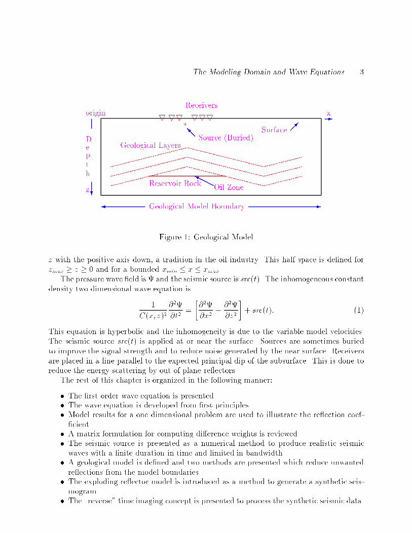
The Modeling Domain and Wave Equations �

Receivers

� ��kk

Source �Buried��I

��Surface ��

�

Depth

�xorigin

z

Geological Layers

��

��

��

��

��

��

XXXXXXXXXXXX

XXXXXXXXXXXX

XXXXXXXXXXXX

��

��

��

Reservoir Rock Oil ZoneHHHY

Geological Model Boundary� �

Figure � Geological Model

z with the positive axis down� a tradition in the oil industry This half space is de�ned forzmax � z � � and for a bounded xmin � x � xmax

The pressure wave �eld is � and the seismic source is src�t� The inhomogeneous constantdensity two dimensional wave equation is

�

C�x� z��

�t��

��

�x��

�z�

�� src�t��

This equation is hyperbolic and the inhomogeneity is due to the variable model velocitiesThe seismic source src�t� is applied at or near the surface Sources are sometimes buriedto improve the signal strength and to reduce noise generated by the near surface Receiversare placed in a line parallel to the expected principal dip of the subsurface This is done toreduce the energy scattering by out of plane re�ectors

The rest of this chapter is organized in the following manner

� The �rst order wave equation is presented� The wave equation is developed from �rst principles� Model results for a one dimensional problem are used to illustrate the re�ection coef�

�cient� A matrix formulation for computing di�erence weights is reviewed� The seismic source is presented as a numerical method to produce realistic seismic

waves with a �nite duration in time and limited in bandwidth� A geological model is de�ned and two methods are presented which reduce unwanted

re�ections from the model boundaries� The exploding re�ector model is introduced as a method to generate a synthetic seis�

mogram� The �reverse� time imaging concept is presented to process the synthetic seismic data

�

t

�� Origin

��

��

��

��

x� x� x� x��t � �� x � xi�� i � ��

� x

� t � x� t �c

Figure � First Order Wave Equation

� The seismic modeling and imaging codes are introduced with operating instructionsand several example models

The seismic data are too complex to visualize as numbers so visualization tools are providedto help in understanding the modeling and imaging process

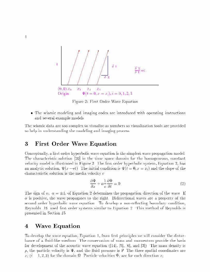
� First Order Wave Equation

Conceptually� a �rst order hyperbolic wave equation is the simplest wave propagation modelThe characteristic solution �� in the time�space domain for the homogeneous� constantvelocity model is illustrated in Figure � The �rst order hyperbolic system� Equation �� hasan analytic solution� ��x� ct� The initial condition is ��t � �� x � xi� and the slope of thecharacteristic solution is the media velocity c

��

�x� �

�

c

��

�t� � ��

The sign of �� of Equation � determines the propagation direction of the wave If� is positive� the wave propagates to the right Bidirectional waves are a property of thesecond order hyperbolic wave equation To develop a non�re�ecting boundary condition�Reynolds �� used �rst order systems similar to Equation � This method of Reynolds ispresented in Section ��

� Wave Equation

To develop the wave equation� Equation �� from �rst principles we will consider the distur�bance of a �uid�like medium The conservation of mass and momentum provide the basisfor development of the acoustic wave equation � �� and �� The mass density is�� the particle velocity is �� and the �uid pressure is P The three spatial coordinates arexi �i � �� for the domain � Particle velocities �i are for each direction xi

Wave Equation �

The conservation of momentum is

��i

�xj�j �

��i

�t� ��ij

�xj� ��

The conservation of mass� the continuity equation� is

��i

�xi��

�t� ��

The incompressible �uid �ow equation can be derived from the Navier�Stokes equations Theform used here is Euler�s equation when the viscosity is zero and uses D as the SubstantialDerivative

�D�

Dt� fb �rP� ��

The body forces are negligible� fb � � Notice that the repeated index used in the equationsindicate a tensor summation

The force S�t� in Equation � acts as a source function upon the domain � Any forceacting within the domain causes pressure and density changes� and the �uid nature of themedium will create an equilibrium restoring force These changes in density and pressureare small

��i

�xj�j �

��i

�t�

�P

�xi� S�t��

We consider small perturbations � in the density �� the particle velocity �� and thepressure P from the initial rest conditions which are labeled with subscript � The perturba�tion Equations � �� and � are for �t� �t� and Pt� the particle velocity� density� and pressurerespectively

�t � ��

�t � ��

Pt � P� ��P ��

The initial particle velocity is �� because the domain � is at restThe density perturbation is known as the acoustic approximation �� A �uid has a

pressure which is a function of density� temperature� and gravity forces We shall assume thatthe gravity forces are relatively constant over the domain � and do not exert any di�erentialforce on the �uid The earth temperature �eld does vary as a function of position and intime� but the temperature changes are very small compared to the time it takes to makeseismic measurements Hence� we will assume that only the density is important and thatthe stress within the �uid is related to the strain as a function of density

First� �ij is de�ned as the Kronecker delta function�

�ij �

�B� � � �

� � ��

�CA ��

�

The stress matrix is �ij�ij � �P ��ij ��

Now using Euler�s Equation �Eq �� with the neglected body forces

�D�

Dt� �rPt� ��

and realizing that P� is constant� we have

�D�

Dt� �r�P� ��

Now the initial medium is at rest and has no convective acceleration� which permits changingthe form of the derivatives in Equation ��

��

�t� �r�P� ��

Next � is the gradient of !� and we can also appreciate that the product of �� and thegradient of ! will be small

r! � � ��

and

��r!

�t� �r�P� ��

Next we assume the derivatives of time and space can be exchanged

r��!�t

� �r�P� ��

Removing the operator � gives

��!

�t� ��P� ��

The compressibility C and the bulk modulus of elasticity K are de�ned in terms of a unitvolume V and �V

C ��

�� V

V��

�P � �K�V

V��

��P � K��

��

Now computing the derivative with respect to time in Equation �� the change in pressureis related to the change in density

��P

�t�

K

��

��

�t��

One Dimensional Problem

r�! � � �

K

��P

�t� ��

Using Equation � to conserve mass and Equations � and ��

��i

�xi� ��

�t� ��r�!� ��

Taking the time derivative of Equation ��

�

�t��!

�t� ��P

�t� ��

Finally� the acoustic wave equation is

r�! ��

v��!

�t��

where v �q

K

��is the sound speed of the medium

� One Dimensional Problem

The one dimensional wave equation with a homogeneous velocity function has an analyticsolution �� The wave propagates in two directions� solutions are of the form ��x� ct� ��x � ct� The method of characteristics can be used to formulate this analytic solutionThe numerical solution �� has the advantage of solving the inhomogeneous problem� whichis awkward analytically but feasible in one dimension After mastering the requirements ofone dimensional modeling� the extensions required for two and three dimensional models arenot di�cult Inhomogeneous modeling in two and three dimensions requires a numericalmethod� analytic methods are not capable of modeling most complex media

�

C�x��

�t��

��

�x�

�� src�t��

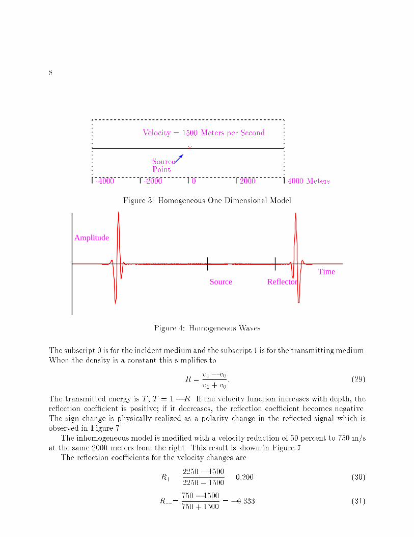
The model used to demonstrate the propagation of waves in one dimension is shown inFigure � The source is placed at the center and the signal is propagated in both directionsfrom the source This model is symmetric and is homogeneous No re�ected waves will begenerated and this wave is plotted at time equals �� seconds as displayed in Figure �

If the model is modi�ed� assume that the velocity is increased by �� percent to the right�� meters from the source Then when the initial source wave impinges on the impedancea re�ected wave will be generated This inhomogeneous model is plotted in Figure � and theseismic waves are plotted in Figure � The strength of the re�ected wave is determined bythe re�ection coe�cient �� Given the velocities and densities the re�ection coe�cient R is

R ��v� � ��v��v� � ��v�

� ��

�

�

�� Meters

SourcePoint

��

Velocity � �� Meters per Second

Figure � Homogeneous One Dimensional Model

Time

Amplitude

Source Reflector

Figure � Homogeneous Waves

The subscript � is for the incidentmediumand the subscript � is for the transmitting mediumWhen the density is a constant this simpli�es to

R �v� � v�v� � v�

� ��

The transmitted energy is T � T � � � R If the velocity function increases with depth� there�ection coe�cient is positive� if it decreases� the re�ection coe�cient becomes negativeThe sign change is physically realized as a polarity change in the re�ected signal which isobserved in Figure

The inhomogeneous model is modi�ed with a velocity reduction of �� percent to �� m"sat the same �� meters from the right This result is shown in Figure

The re�ection coe�cients for the velocity changes are

R� ��

��

R�

� ��

��

One Dimensional Problem �

�

�� Meters

SourcePoint

��

Velocity � �� Meters per Second Velocity � ��

Re�ector��

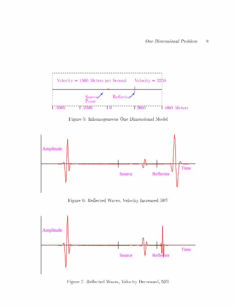
Figure � Inhomogeneous One Dimensional Model

Time

Amplitude

Source Reflector

Figure � Re�ected Waves� Velocity Increased ��#

Time

Amplitude

Source Reflector

Figure Re�ected Waves� Velocity Decreased� ��#

��

The corresponding transmission coe�cients for the velocity changes are

T� � ��R� � ��

T�

� ��R�

� ��

If we examine Figures � and � the re�ections show both the amplitude di�erences and thesign di�erences of Equations �� and �� Likewise� the transmission coe�cients of Equations�� and �� compare well with the �gures

� Derivative Coe�cients

The time and space derivatives must be discretized from a continuous function to a discretefunction Methods used to compute derivatives for seismic modeling include Taylor Series�Chebechev� Fourier Transforms� and Pad$e The Taylor Series �TS� methods will be developedhere� they are reasonably good approximations but not optimal The theories for optimaloperators are beyond the scope of this e�ort The TS method assumes that a functionknown at point a can be extended to point b if su�cient number of derivatives exist and areknown at point a The truncation error for the series expansion has a maximum within theapproximation interval

The formulation preferred is a matrix representation for computing the coe�cients of theTaylor Series Given

h � b� a ��

then

f�b� � f�a� � f�

�a�h�f

��

�a�h�

�%�f

��

�a�h�

�%� � � ��

This computation of f�b� does not explain how to compute a derivative approximationBut if the point b is extended to a series of uniformly spaced points each a multiple of hfrom a and we write the TS expansion as an expression� we get

f�h�f��f��h�

��

f�� f�

��h �f

��

��h�

��

f��

f�� f �

��h �f

��

��h�

��

��

Assume the di�erence operator is centered at the origin Now formulating this as a matrixequation using terms up to the second derivative� we have

�B� f�h�

f��f��h�

�CA �

�B� � h h�

�

� � �

� �h h�

�

�CA�B�

f��f

�

��f

��

��

�CA ��

Seismic Source Function ��

Thus an invertible matrix equation is generated Care must be taken to use an appro�priate value for h� the simplest method is to factor the h terms out with the functionsOtherwise� for longer operators the matrix can be numerically unstable and di�cult to in�vert The h terms contribute to a poor condition number matrix The result is general andwill generate di�erence operators for any length

Solving Equation � for the f�� and derivative terms gives

�B�

f��f

�

��f

��

��

�CA �

�

h�

�B�

� h� �h

�� h

�

� ��

�CA�B�

f�h�f��f��h�

�CA ��

If we modify the matrix terms by factoring out the terms in h in Equation � � we get asimpler matrix which will have a better condition number

�B� f�h�

f��f��h�

�CA �

�B� � � �

�

� � ��

�

�CA�B�

f��h�

f�

��h�

f��

��h�

�CA ��

This can be solved like Equation �� and we see the familiar weights for the �rst andsecond derivatives �

B�f��h�

f�

��h�

f��

��h�

�CA �

�B� � � �

��

�

� ��

�CA�B� f�h�

f��f��h�

�CA ��

The second derivative equation is

f��

��

h� f�h�� f�� f��h��

The coe�cients for the derivative approximations with di�erent grid spacings� or with moregrid points� can be computed with this method

� Seismic Source Function

To generate seismic waves a source function is required This section develops the conceptof a frequency band limited source function Real seismic sources use an energy impulseor a vibration source to generate waves in the earth Impulse sources include dynamite� adrop weight� a sledge hammer� a shot gun� or a ri�e The actual source used is dependenton the desired signal to noise ratio� the human environment� the target depth desired andthe geological environment The vast majority of land seismic data are generated by twomethods� dynamite placed in shot holes drilled into the earth or by a truck mounted vibratingmass which shakes the earth in a vertical or horizontal direction The method we will use inour simulation of seismic exploration is the impulsive dynamite source

��

Time

Amplitude

Figure � Source Function

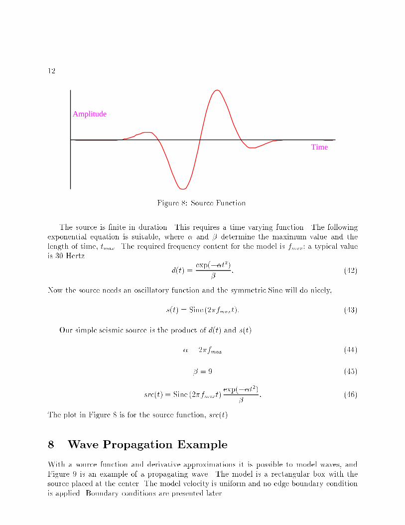
The source is �nite in duration This requires a time varying function The followingexponential equation is suitable� where � and � determine the maximum value and thelength of time� tmax The required frequency content for the model is fmax� a typical valueis �� Hertz

d�t� �exp��t��

��

Now the source needs an oscillatory function and the symmetric Sine will do nicely�

s�t� � Sine ��fmaxt��

Our simple seismic source is the product of d�t� and s�t�

� � ��fmax ��

� � � ��

src�t� � Sine ��fmaxt�exp��t��

��

The plot in Figure � is for the source function� src�t�

� Wave Propagation Example

With a source function and derivative approximations it is possible to model waves� andFigure � is an example of a propagating wave The model is a rectangular box with thesource placed at the center The model velocity is uniform and no edge boundary conditionis applied Boundary conditions are presented later

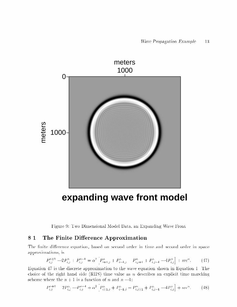
Wave Propagation Example ��

0

1000

met

ers

1000meters

expanding wave front model

Figure � Two Dimensional Model Data� an Expanding Wave Front

�� The Finite Di�erence Approximation

The �nite di�erence equation� based on second order in time and second order in spaceapproximations� is

P n��i�j � �P n

i�j � P n��i�j � ��

hP ni��j � P n

i��j � P ni�j�� P n

i�j�� P ni�j

i� srcn� ��

Equation � is the discrete approximation to the wave equation shown in Equation � Thechoice of the right hand side �RHS� time value as n describes an explicit time marchingscheme where the n� � is a function of n and n� �


i�j � P n��i�j � ��




i� srcn� ��

��

Origin

Z

X

�

�

dz

dx

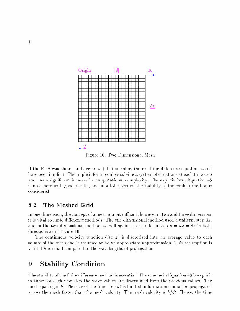
Figure �� Two Dimensional Mesh

If the RHS was chosen to have an n� � time value� the resulting di�erence equation wouldhave been implicit The implicit form requires solving a system of equations at each time stepand has a signi�cant increase in computational complexity The explicit form Equation ��is used here with good results� and in a later section the stability of the explicit method isconsidered

�� The Meshed Grid

In one dimension� the concept of a mesh is a bit di�cult� however in two and three dimensionsit is vital to �nite di�erence methods The one dimensional method used a uniform step dx�and in the two dimensional method we will again use a uniform step h � dx � dz in bothdirections as in Figure ��

The continuous velocity function C�x� z� is discretized into an average value to eachsquare of the mesh and is assumed to be an appropriate approximation This assumption isvalid if h is small compared to the wavelengths of propagation

Stability Condition

The stability of the �nite di�erence method is essential The scheme in Equation �� is explicitin time� for each new step the wave values are determined from the previous values Themesh spacing is h The size of the time step dt is limited� information cannot be propagatedacross the mesh faster than the mesh velocity The mesh velocity is hdt Hence� the time

Seismic Modeling in Two Dimensions ��

step �t must be bounded� and for the di�erence equation this limit is

c�t

h� �p

nd��

where nd is the number of spatial dimensionsIn two dimensions the stability condition is

c�t

h� �p

��

The maximum time step size is bounded by

�t � h

cp��

� Seismic Modeling in Two Dimensions

�� Shot Record Modeling

Assuming a model velocity structure C�x� z� is known and the source location Sshot�x� z� isspeci�ed� it is possible to simulate a sequence of shot records These individual shot recordsare recorded as data Dshot�x� t� and processed like �eld data

The geometry of the source location� the receiver separation� and the number of receiversused depends on a number of factors Close sample spacing in the seismic experimentprovides better data quality and improves the signal to noise ratio The subsurface structurescatters energy in di�erent directions If the structure has signi�cant dip then long receiverspreads are used The cost of shots and drill holes also in�uences the geometry of seismicdata collection

These geometry considerations are not as critical in seismic modeling because the physical�eld constraints do not apply The amount of data generated by a seismic model can be aproblem� and it is not always wise to record every grid point along the receiver line for everytime step Su�cient data must be recorded to prevent aliasing the data �� the Nyquistlimit is two grid points per wave length Care must be taken to collect data which is notaliased either in space or time While two grid points per wavelength is the theoretical limit�careful experimenters use at least three

The routine seismic processing sequence will attempt to �atten the time recordings andsum into a stack section This stacking process reduces the amount of data by a signi�cantamount The individual shot records are corrected for o�set� the distance from the sourcelocation� and then summed This process is termed a moveout correction The equivalentseismic process would be to use only one receiver for every shot point location and record thisdata This coincident source and receiver position is known as zero�o�set data and wouldnot need moveout correction

��

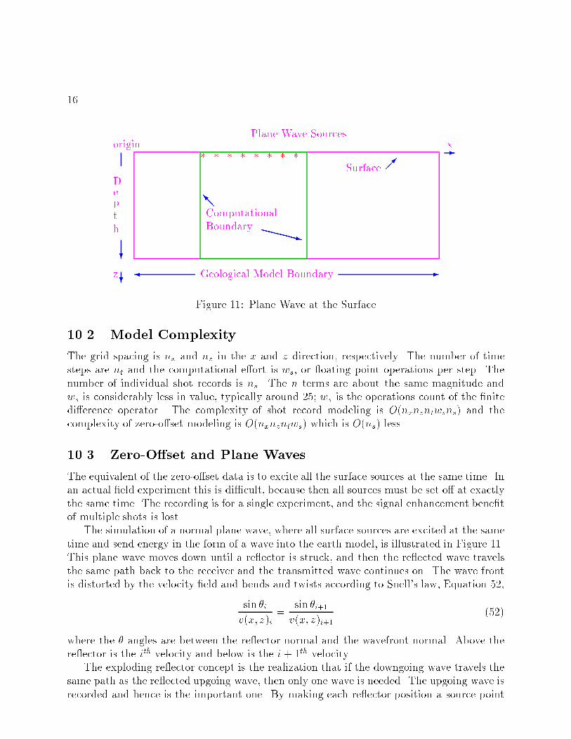
Plane Wave Sources

� � � � � � � �Surface ��

�

Depth

�xorigin

�z

ComputationalBoundary

��I

XXXXXz


Figure �� Plane Wave at the Surface

�� Model Complexity

The grid spacing is nx and nz in the x and z direction� respectively The number of timesteps are nt and the computational e�ort is ws� or �oating point operations per step Thenumber of individual shot records is ns The n terms are about the same magnitude andws is considerably less in value� typically around �� ws is the operations count of the �nitedi�erence operator The complexity of shot record modeling is O�nxnzntwsns� and thecomplexity of zero�o�set modeling is O�nxnzntws� which is O�ns� less

�� Zero�O�set and Plane Waves

The equivalent of the zero�o�set data is to excite all the surface sources at the same time Inan actual �eld experiment this is di�cult� because then all sources must be set o� at exactlythe same time The recording is for a single experiment� and the signal enhancement bene�tof multiple shots is lost

The simulation of a normal plane wave� where all surface sources are excited at the sametime and send energy in the form of a wave into the earth model� is illustrated in Figure ��This plane wave moves down until a re�ector is struck� and then the re�ected wave travelsthe same path back to the receiver and the transmitted wave continues on The wave frontis distorted by the velocity �eld and bends and twists according to Snell�s law� Equation ��

sin iv�x� z�i

�sin i��

v�x� z�i��

where the angles are between the re�ector normal and the wavefront normal Above there�ector is the ith velocity and below is the i� �th velocity

The exploding re�ector concept is the realization that if the downgoing wave travels thesame path as the re�ected upgoing wave� then only one wave is needed The upgoing wave isrecorded and hence is the important one By making each re�ector position a source point

Seismic Modeling in Two Dimensions �

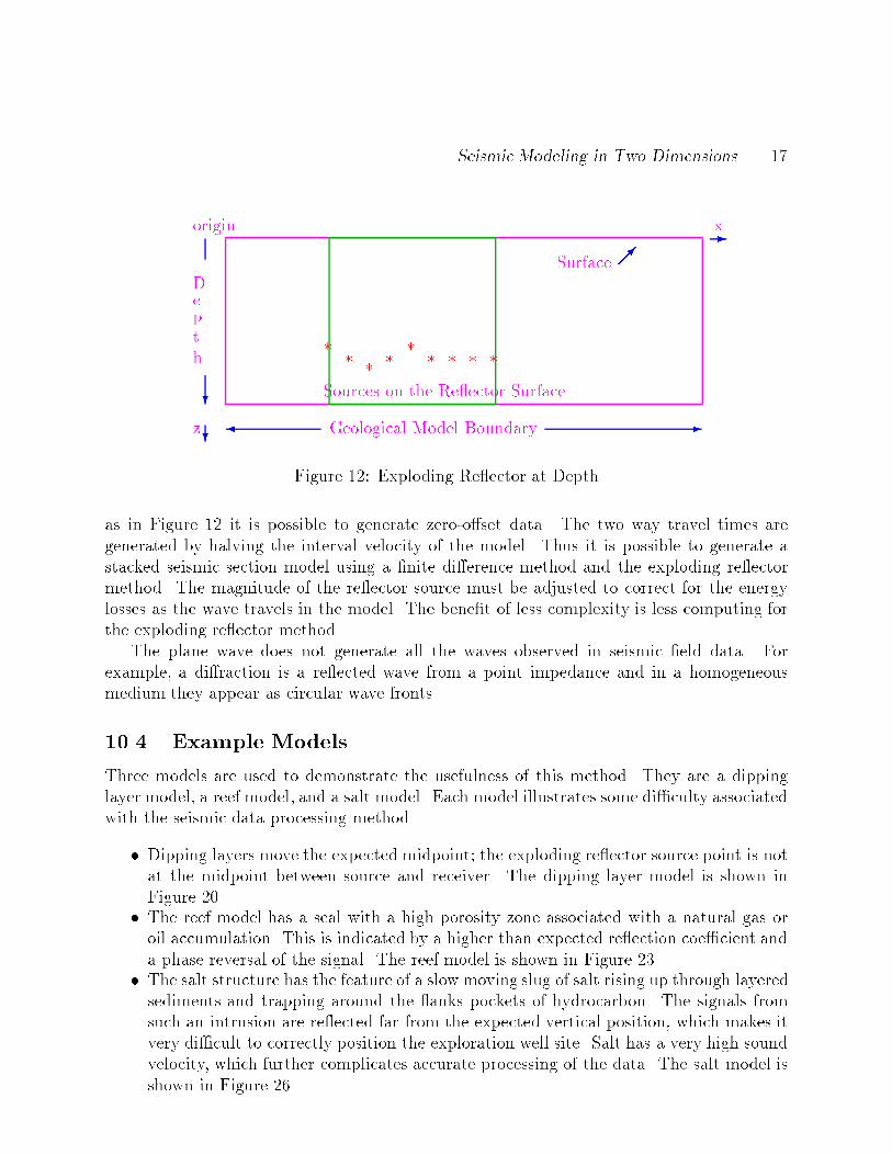
Sources on the Re�ector Surface

� � � � � � � � �

Surface ��

�

Depth

�xorigin

�z Geological Model Boundary� �

Figure �� Exploding Re�ector at Depth

as in Figure �� it is possible to generate zero�o�set data The two way travel times aregenerated by halving the interval velocity of the model Thus it is possible to generate astacked seismic section model using a �nite di�erence method and the exploding re�ectormethod The magnitude of the re�ector source must be adjusted to correct for the energylosses as the wave travels in the model The bene�t of less complexity is less computing forthe exploding re�ector method

The plane wave does not generate all the waves observed in seismic �eld data Forexample� a di�raction is a re�ected wave from a point impedance and in a homogeneousmedium they appear as circular wave fronts

�� Example Models

Three models are used to demonstrate the usefulness of this method They are a dippinglayer model� a reef model� and a salt model Each model illustrates some di�culty associatedwith the seismic data processing method

� Dipping layers move the expected midpoint� the exploding re�ector source point is notat the midpoint between source and receiver The dipping layer model is shown inFigure ��

� The reef model has a seal with a high porosity zone associated with a natural gas oroil accumulation This is indicated by a higher than expected re�ection coe�cient anda phase reversal of the signal The reef model is shown in Figure ��

� The salt structure has the feature of a slow moving slug of salt rising up through layeredsediments and trapping around the �anks pockets of hydrocarbon The signals fromsuch an intrusion are re�ected far from the expected vertical position� which makes itvery di�cult to correctly position the exploration well site Salt has a very high soundvelocity� which further complicates accurate processing of the data The salt model isshown in Figure ��

��

After studying the seismic modeling process we shall �nd a way to process this zero�o�setdata and image it This imaging process we shall call migration� the e�ect of moving datamispositioned in time to a place in depth The exploding re�ector modeling data are plottedin Figures �� and � for the dipping layer� reef� and salt models� respectively

�� Model Building

The models are simple line segments with a z�intercept and a slope and overlapped circlesplaced in sequence Each interface line segment is used as a boundary and all velocity gridvalues below the line segment are changed to the new value The circles are used to modifythese grid values� with all points within the circle of speci�ed radius and origin acquiring anew velocity value The sequence of lines and circles can vary to create interesting models

�� Imaging� Two Dimensions

The partial di�erential equation for modeling� the wave equation� assumes a quiet backgroundas the initial condition What would happen if the recorded seismic data were introduced intothe wave equation as a boundary condition The data would propagate into the earth fromthe receiver positions very much like the exploding re�ector model process if the re�ectorwas at the surface If the wave equation is formulated as a backward in time equation� theboundary condition data can be moved down in depth until time reaches zero This zerotime is called the imaging condition� t � �

We shall see that this method works and propagates the surface recorded data back intodepth What is missing is the energy which left the sides and bottom of the image �eld Itis possible to record along the sides of an image �eld� but this is not done very often Thebottom data are quite di�cult and expensive to obtain Essentially� the only data routinelyavailable are the surface seismic shot record data� which is stacked to improve the signalto noise ratio This stacked data can then be migrated Sounds so simple� but what is theearth velocity model to be used& If we examine Equation �� we see that the velocity termis essential We shall assume the velocities are known

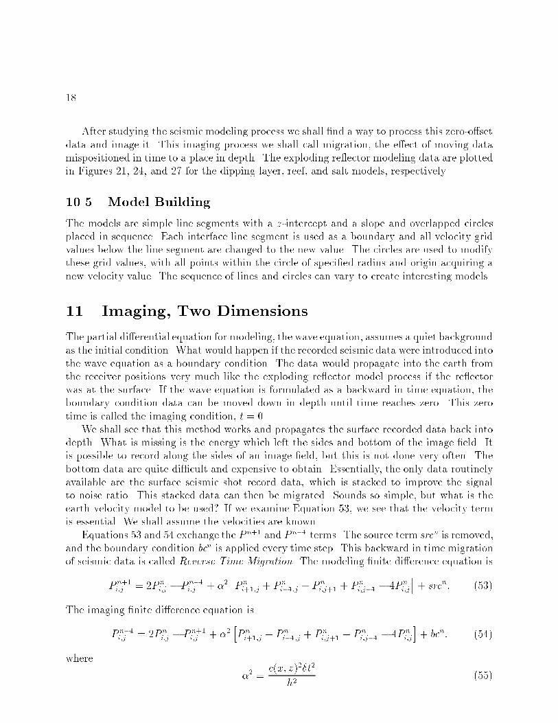
Equations �� and �� exchange the P n�� and P n�� terms The source term srcn is removed�and the boundary condition bcn is applied every time step This backward in time migrationof seismic data is called Reverse Time Migration The modeling �nite di�erence equation is


i�j � P n��i�j � ��




i� srcn� ��

The imaging �nite di�erence equation is


i�j � P n��i�j � ��




i� bcn� ��

where

�� c�x� z��t�

h��

Seismic Data Display ��

The three seismic models which were generated using the exploding re�ector model aremigrated using Equation �� The dipping layer� reef� and salt models have all been computedusing the initial known velocity model and are shown in Figures �� and �� respectivelyStudy the moving wave �elds and see if the recorded re�ections move into the earth in anunderstandable way As you might want to compare the migration process with the modelingprocess� notice that waves exiting the model sides do not appear in the migration What doesthis do to the image reconstruction& Would any other imaging method be more successfulin reconstruction of the missing data&

Obtaining velocity data for the model is the next step in the process Let�s begin witha simple marine data case� data which was collected over water The velocity of water isapproximately �� meters per second Only the depth of the water is unknown and can becomputed from the seismic data

However� on land we are in for a terrible surprise The weathered earth is just that� andthe low velocity layer has truly variable properties Just look across your favorite park andyou will see stream beds with sand and gravel� hills with bedrock� fertile �elds with soils� allplaces where the earth is really di�erent All these di�erences are seen in the near surfaceseismic data Here both the velocity and depth are unknown and will be determined fromthe seismic data

After the �rst layer either on land or at sea we still have mystery to unravel what is thevelocity of the rest of the subsurface& This we shall leave for another day I will say thatusing the unstacked data and more powerful mathematics it is possible to do a very crediblejob of velocity analysis

�� Seismic Data Display

An X�windows tool Suxwigb is available from the Center for Wave Phenomena at ColoradoSchool of Mines Seismic Unix� or SU� is a public domain seismic trace processing packageof which Suxwigb is a part

This seismic trace display has the ability to display wiggle traces and in"out zoom Thisis a public domain software product and is included with the codes of this chapter Theinput �le required by Suxwigb is generated by ftn�su and is an unformatted Fortran �leThe Ftn�su �le is a formatted Fortran �le organized trace by trace These input �les arequite large and SU permits Unix piping of process output

The reader is encouraged to test seismic display before proceeding

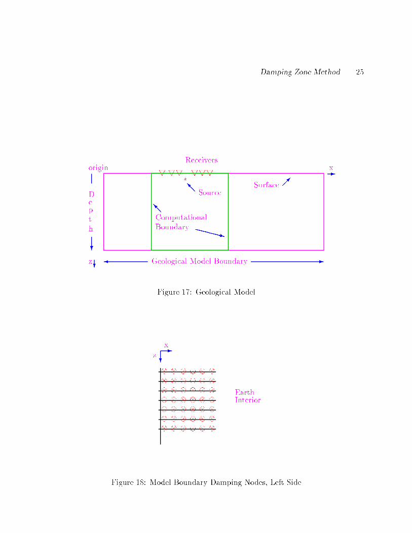
�� Introduction to Boundary Conditions

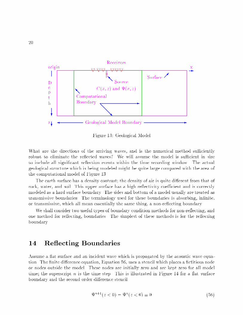
The model con�guration in Figure �� describes a �nite bounded area in two dimensionsWhen a propagated wave arrives in the neighborhood of the boundary� we must considerthe e�ects of the re�ected wave Are re�ected waves wanted& Is a re�ected wave a physicalphenomenon� or is it an artifact& What are the consequences of the �nite nature of the model&

��

Receivers

� ��kk

Source��I


�

Depth

�xorigin

�z


��I

��R


C�x� z� and ��x� z�

Figure �� Geological Model

What are the directions of the arriving waves� and is the numerical method su�cientlyrobust to eliminate the re�ected waves& We will assume the model is su�cient in sizeto include all signi�cant re�ection events within the time recording window The actualgeological structure which is being modeled might be quite large compared with the area ofthe computational model of Figure ��

The earth surface has a density contrast� the density of air is quite di�erent from that ofrock� water� and soil This upper surface has a high re�ectivity coe�cient and is correctlymodeled as a hard surface boundary The sides and bottom of a model usually are treated astransmissive boundaries The terminology used for these boundaries is absorbing� in�nite�or transmissive� which all mean essentially the same thing� a non�re�ecting boundary

We shall consider two useful types of boundary condition methods for non�re�ecting� andone method for re�ecting� boundaries The simplest of these methods is for the re�ectingboundary

�� Re�ecting Boundaries

Assume a �at surface and an incident wave which is propagated by the acoustic wave equa�tion The �nite di�erence equation� Equation �� uses a stencil which places a �ctitious nodeor nodes outside the model These nodes are initially zero and are kept zero for all modeltime� the superscript n is the time step This is illustrated in Figure �� for a �at surfaceboundary and the second order di�erence stencil

�n��z � �� n�z � ��

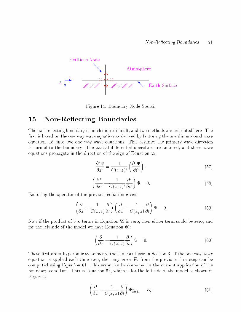
Non�Re�ecting Boundaries ��

Fictitious Node

��R Atmosphere

Earth Surface��I�

�

xz

��

Figure �� Boundary Node Stencil

�� Non Re�ecting Boundaries

The non�re�ecting boundary is muchmore di�cult� and two methods are presented here The�rst is based on the one way wave equation as derived by factoring the one dimensional waveequation �� into two one way wave equations This assumes the primary wave directionis normal to the boundary The partial di�erential operators are factored� and these waveequations propagate in the direction of the sign of Equation ��

��

�x��

�

C�x� z��

��

�t�

��

��

�x��

C�x� z��

�t�

��

Factoring the operator of the previous equation gives

��

�x�

�

C�x� z�

�

�t

��

�x� �

C�x� z�

�

�t

��

Now if the product of two terms in Equation �� is zero� then either term could be zero� andfor the left side of the model we have Equation ��

��

�x� �

C�x� z�

�

�t

��

These �rst order hyperbolic systems are the same as those in Section � If the one way waveequation is applied each time step� then any error Er from the previous time step can becomputed using Equation �� This error can be corrected in the current application of theboundary condition This is Equation �� which is for the left side of the model as shown inFigure ��

��

�x� �

C�x� z�

�

�t

��n

x��x� Er� ��

��

EarthInterior

�

�

x

z

Node Numbers��

�x �x

Figure �� Model Boundary Node Stencil� Left Side

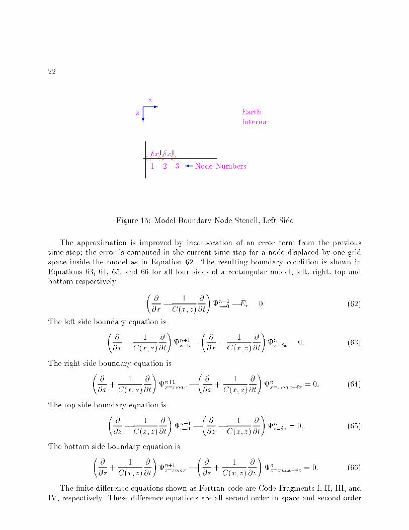
The approximation is improved by incorporation of an error term from the previoustime step� the error is computed in the current time step for a node displaced by one gridspace inside the model as in Equation �� The resulting boundary condition is shown inEquations �� and �� for all four sides of a rectangular model� left� right� top andbottom respectively

��

�x� �

C�x� z�

�

�t

��n��

x�� Er � ��

The left side boundary equation is��

�x� �

C�x� z�

�

�t

��n��

x��

�x� �

C�x� z�

�

�t

��n

x��x � ��

The right side boundary equation is��

�x�

�

C�x� z�

�

�t

��n��

x�xmax ��

�x�

�

C�x� z�

�

�t

��n

x�xmax��x � ��

The top side boundary equation is��

�z� �

C�x� z�

�

�t

��n��

z��

�z� �

C�x� z�

�

�t

��n

z��z � ��

The bottom side boundary equation is��

�z�

�

C�x� z�

�

�t

��n��

z�zmax ��

�z�

�

C�x� z�

�

�z

��n

z�zmax��z � ��

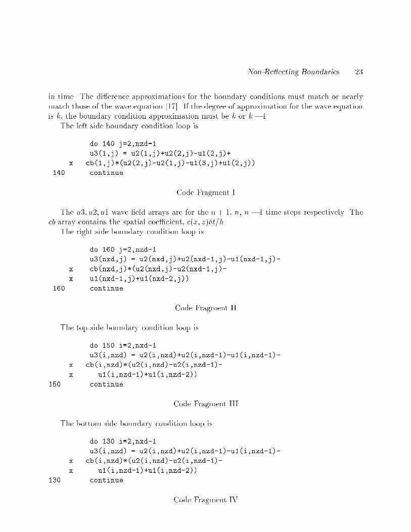
The �nite di�erence equations shown as Fortran code are Code Fragments I� II� III� andIV� respectively These di�erence equations are all second order in space and second order

Non�Re�ecting Boundaries ��

in time The di�erence approximations for the boundary conditions must match or nearlymatch those of the wave equation � � If the degree of approximation for the wave equationis k� the boundary condition approximation must be k or k � �

The left side boundary condition loop is

do �� j��nzd��

u��j � u��ju��j�u��j

x cb��j��u��j�u��j�u��ju��j

�� continue

Code Fragment I

The u�� u�� u� wave �eld arrays are for the n � �� n� n � � time steps respectively Thecb array contains the spatial coe�cient� c�x� z��th

The right side boundary condition loop is

do �� j��nzd��

u��nxd�j � u��nxd�ju��nxd��j�u��nxd��j�

x cb�nxd�j��u��nxd�j�u��nxd��j�

x u��nxd��ju��nxd��j

�� continue

Code Fragment II

The top side boundary condition loop is

do � � i��nxd��

u��i�nzd � u��i�nzdu��i�nzd��u��i�nzd��

x cb�i�nzd��u��i�nzd�u��i�nzd��

x u��i�nzd��u��i�nzd��

� � continue

Code Fragment III

The bottom side boundary condition loop is

do �� i��nxd��

u��i�nzd � u��i�nzdu��i�nzd��u��i�nzd��

x cb�i�nzd��u��i�nzd�u��i�nzd��

x u��i�nzd��u��i�nzd��

�� continue

Code Fragment IV

��

Receivers

� ��kk

Source��I


�

Depth

�xorigin

�z


��I

��

ZZZZ�

Damping

ZoneXXXXz

��

��

��

��


Figure �� Computational Model Damping Zone

The di�culty the one way wave equation has for waves which arrive at angles other thannormal could be �xed by making an angle dependent method The wave �eld is used todetermine an incoming wave direction� and the wave �eld is decomposed into two parts�normal and tangential If more than one wave is active in the boundary region� it makes thedirection and decomposition quite complex A considerable amount of work has been donein developing boundary conditions and angle dependent boundary conditions� students arenot encouraged to plow this old ground The damping method� presented next� is suitablefor most modeling methods and overcomes the angle dependent di�culty in an elegant way��it does not care where the wave comes from� Further� it is independent of the degree ofapproximation for the wave equation

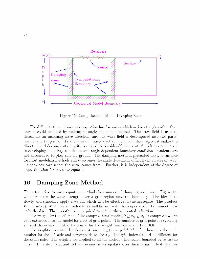
�� Damping Zone Method

The alternative to wave equation methods is a numerical damping zone� as in Figure ��which reduces the wave strength over a grid region near the boundary The idea is toslowly and smoothly apply a weight which will be e�ective in the aggregate The productW � 'w�xw��W � �� is computed to a small factor � with the property of certain smoothnessat both edges The smoothness is required to reduce the unwanted re�ections

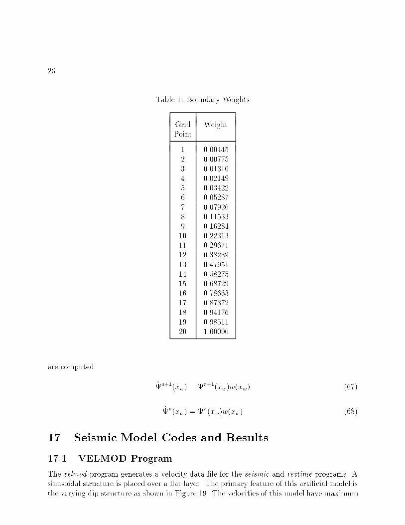
The weight for the left side of the computational model� � � xw � xb� is computed wherexb is extended into the model for a set of grid points The number of grid points is typically�� and the values of Table � are used for the weight function where W � ��

The weights presented by Cerjan �� are w�xw� � exp��i�

� where i is the nodenumber for the left side and corresponds to the xw The grid index i could be di�erent forthe other sides The weights are applied to all the nodes in the region bounded by xb to thecurrent time step data� and to the previous time step data after the interior �nite di�erences

Damping Zone Method ��

Receivers

� ��kk

Source��I


�

Depth

�xorigin

�z


��I

XXXXXz


Figure � Geological Model

InteriorEarth

�

�

x

z

Figure �� Model Boundary Damping Nodes� Left Side

��

Table � Boundary Weights

Grid WeightPoint

� ��

are computed

(�n��xw� � �n��xw�w�xw� ��

(�n�xw� � �n�xw�w�xw� ��

�� Seismic Model Codes and Results

�� VELMOD Program

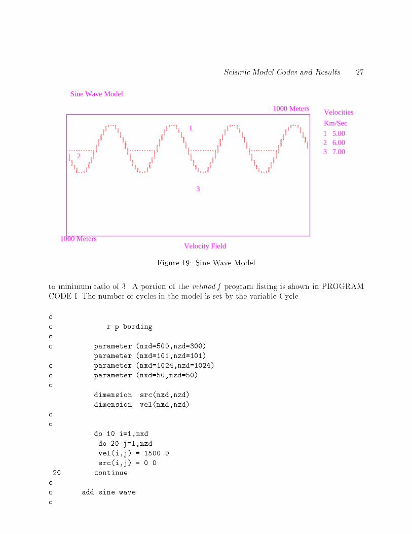
The velmod program generates a velocity data �le for the seismic and revtime programs Asinusoidal structure is placed over a �at layer The primary feature of this arti�cial model isthe varying dip structure as shown in Figure �� The velocities of this model have maximum

Seismic Model Codes and Results �

Velocity Field

Sine Wave Model

1000 Meters

1000 Meters

Velocities

Km/Sec

1 5.00 1

2 6.00

2 3 7.00

3

Figure �� Sine Wave Model

to minimum ratio of � A portion of the velmod�f program listing is shown in PROGRAMCODE I The number of cycles in the model is set by the variable Cycle

c

c r p bording

c

c parameter �nxd� ��nzd��

parameter �nxd��nzd��

c parameter �nxd��nzd��

c parameter �nxd� ��nzd� �

c

dimension src�nxd�nzd

dimension vel�nxd�nzd

c

c

do �� i��nxd

do �� j��nzd

vel�i�j � � ��

src�i�j � ��

�� continue

c

c add sine wave

c

��

xx � i

xt � nxd

xr � xx�xt

n��

jzz � �nzd�n��sin��xr

do � j�jzz�nzd

vel�i�j � ��

� continue

do �� j�jzz��nzd

vel�i�j � � ��

�� continue

�� continue

do �� i�nxd��nxd�nxd��

c

c add sine wave

c

xx � i

xx � xx � ��

xt � nxd

xr � xx�xt

c

jzz � �nzd��cos��xr��

�� continue

c

vmin � vel��

vmax � vel��

do �� i��nxd

do �� j��nzd

if� j �ne� nzd then

if�abs� vel�i�j � vel�i�j� �gt� �� then


endif

endif

if� vel�i�j �gt� vmax vmax � vel�i�j

if� vel�i�j �lt� vmin vmin � vel�i�j

�� continue

�� continue

c

open��file��mvel�dat��form��unformatted�

open��file��velocity�dat��form��unformatted�

do �� i��nzd

Seismic Model Codes and Results ��

write�� vel�j�i�j��nxd

write�� vel�j�i�j��nxd

�� continue

close��

write�� vmin�vmax

�� format� � min� max velocity ��f��

close��

open��file��reflector�dat��form��unformatted�

do �� i��nzd

write�� src�j�i�j��nxd

�� continue

close��

open��file��reflector�su��form��formatted�

la � �

write�� nzd�nxd�la

�� format��i�

do i��nxd

do j��nzd

write�� src�i�j

�� format�e��

enddo

enddo

close��

end

PROGRAM CODE I� Sine Wave Model

�� Dipping Model

�� DIP Program

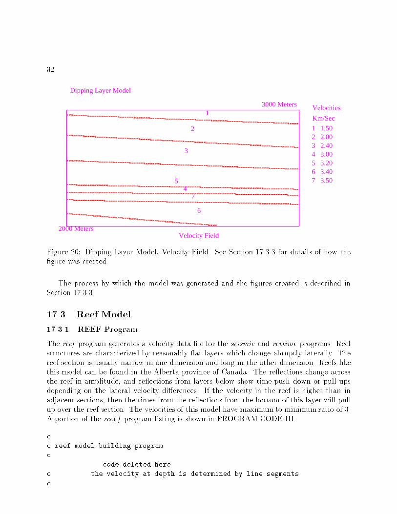
The dip program generates a velocity data �le for the seismic and revtime programs This isthe simplest model provided and illustrates the reverse time method The layers are nearly�at� but some slight dip is included This geology is similar to regions of West Texas Thevelocities of this model have maximumto minimumratio of � A portion of the dip�f programlisting is shown in PROGRAM CODE II

c

c dipping layer model building program

c

c

parameter�nx��nz��

��

c

dimension vv�nx�nz

dimension vz��

c

dimension am��bm��

c

c the velocity at depth is determined by line segments

c

nline � �

c

bm��

bm��

bm��

bm��

bm� � ��

bm��

bm��

bm��

c

c

am��

am��

am��

am��

am� � ��

am��

am��

am��

c

vz��

vz��

vz��

vz��

vz� � � ��

vz��

vz��

vz��

c

dx � � ��

dz � � ��

c

c create initial water layer


c

do i��nx

do j��nz

vv�i�j � � ��

enddo

enddo

c

c now layer by layer make velocities under each

c line

c

c each new layer over writes that below

c

do k��nline

do i��nx

do j��nz

x � �i��dx

z � �j��dz

zl � am�k�x bm�k

c

if� z �gt� zl then

vv�i�j � vz�k

endif

enddo

enddo

enddo

c

c write model to file

c

open��file��dip�dat��form��unformatted�

do j��nz

write�� vv�i�j�i��nx

enddo

close��

end

PROGRAM CODE II� The Dipping Model

�� Dipping Layer Model Results

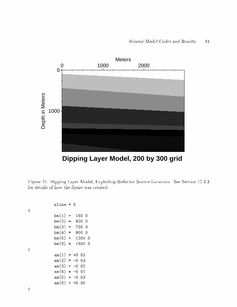
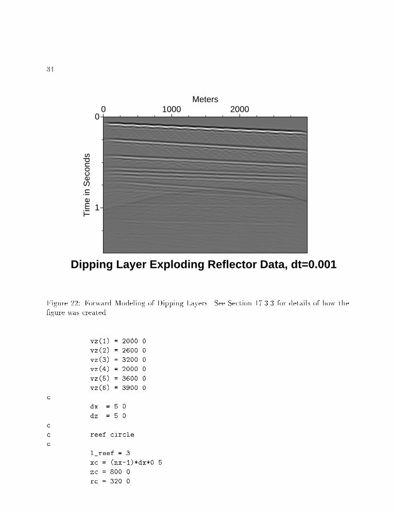
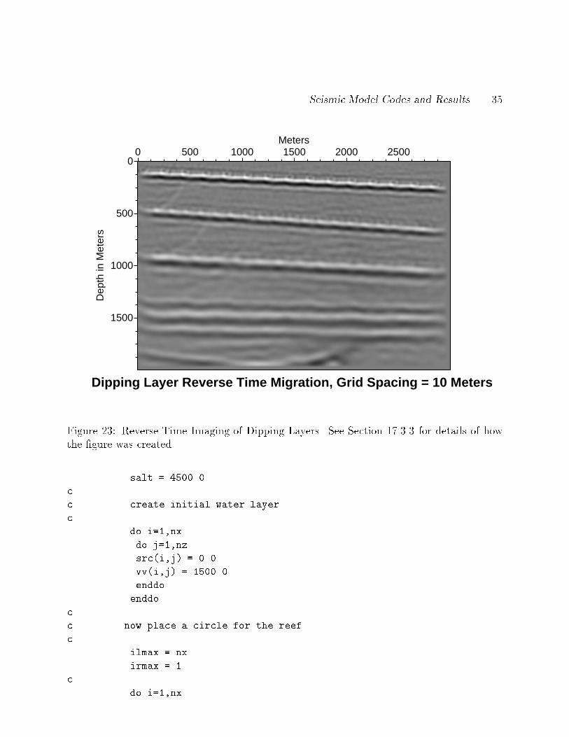
The dipping layer model velocity �eld and exploding re�ector source locations are shown inFigures �� and �� respectively The computed model results are shown in Figures �� and��

��

Velocity Field

Dipping Layer Model

3000 Meters

2000 Meters

Velocities

Km/Sec

1 1.50

1

2 2.00 2

3 2.40 3 4 3.00

4

5 3.20

5 6 3.40

6

7 3.50

7

Figure �� Dipping Layer Model� Velocity Field See Section � �� for details of how the�gure was created

The process by which the model was generated and the �gures created is described inSection � ��

�� Reef Model

�� REEF Program

The reef program generates a velocity data �le for the seismic and revtime programs Reefstructures are characterized by reasonably �at layers which change abruptly laterally Thereef section is usually narrow in one dimension and long in the other dimension Reefs likethis model can be found in the Alberta province of Canada The re�ections change acrossthe reef in amplitude� and re�ections from layers below show time push down or pull upsdepending on the lateral velocity di�erences If the velocity in the reef is higher than inadjacent sections� then the times from the re�ections from the bottom of this layer will pullup over the reef section The velocities of this model have maximum to minimum ratio of �A portion of the reef�f program listing is shown in PROGRAM CODE III

c

c reef model building program

c

�� code deleted here ��


c


0

1000

Dep

th in

Met

ers

0 1000 2000Meters

Dipping Layer Model, 200 by 300 grid

Figure �� Dipping Layer Model� Exploding Re�ector Source Locations See Section � ��for details of how the �gure was created

nline � �

c

bm��

bm��

bm��

bm��

bm� � ��

bm��

c

am��

am��

am��

am��

am� � ��

am��

c

��

0

1

Tim

e in

Sec

onds

0 1000 2000Meters

Dipping Layer Exploding Reflector Data, dt=0.001

Figure �� Forward Modeling of Dipping Layers See Section � �� for details of how the�gure was created

vz��

vz��

vz��

vz��

vz� � ��

vz��

c

dx � ��

dz � ��

c

c reef circle

c

l�reef � �

xc � �nx��dx��

zc � ��

rc � ��


0

500

1000

1500

Dep

th in

Met

ers

0 500 1000 1500 2000 2500Meters

Dipping Layer Reverse Time Migration, Grid Spacing = 10 Meters

Figure �� Reverse Time Imaging of Dipping Layers See Section � �� for details of howthe �gure was created

salt � � ��

c


c

do i��nx

do j��nz


vv�i�j � � ��

enddo

enddo

c

c now place a circle for the reef

c

ilmax � nx

irmax � �

c

do i��nx

��

do j��nz

x � �i��dx

z � �j��dz

r � sqrt��x�xc��z�zc��

c

c if point is inside circle it�s the reef

c

if� r �lt� rc then

if� i �lt� ilmax ilmax � i

if� i �gt� irmax irmax � i

endif

enddo

enddo

c


c line

c


c

do k��nline

do i��nx

do j��nz

x � �i��dx

z � �j��dz

zl � am�k�x bm�k

c


vmult � ��

if�l�reef �eq� k then

if� i �gt� ilmax �and� i �lt� irmax vmult � ��

if� i �gt� irmax vmult � ��

endif

vv�i�j � vz�k�vmult

endif

enddo

enddo

enddo

c


PROGRAM CODE III� The Reef Model

Seismic Model Codes and Results �

Velocity Field

Reef Model

3000 Meters

2000 Meters

Velocities

Km/Sec

1 1.50 1

2 2.00 2 3 2.60

3 4 2.80

4

5 3.20

5

6 3.60

6

7 3.84 7 8 3.90

8

9 4.48

9

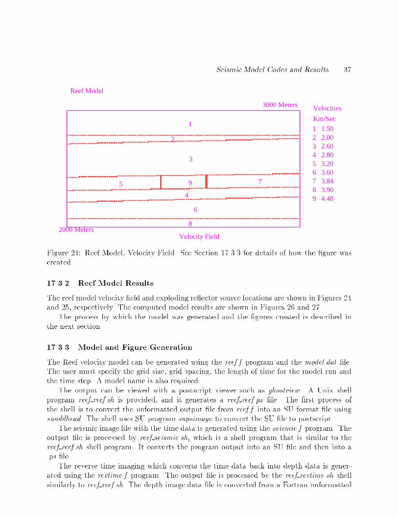
Figure �� Reef Model� Velocity Field See Section � �� for details of how the �gure wascreated

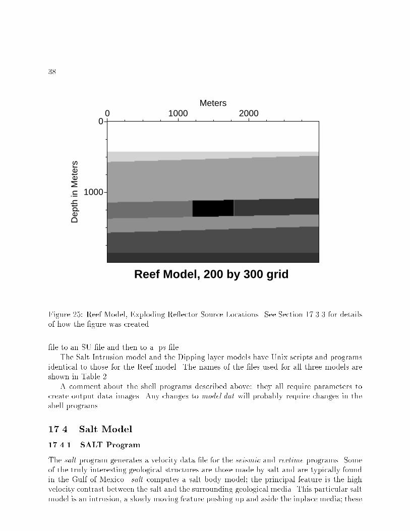
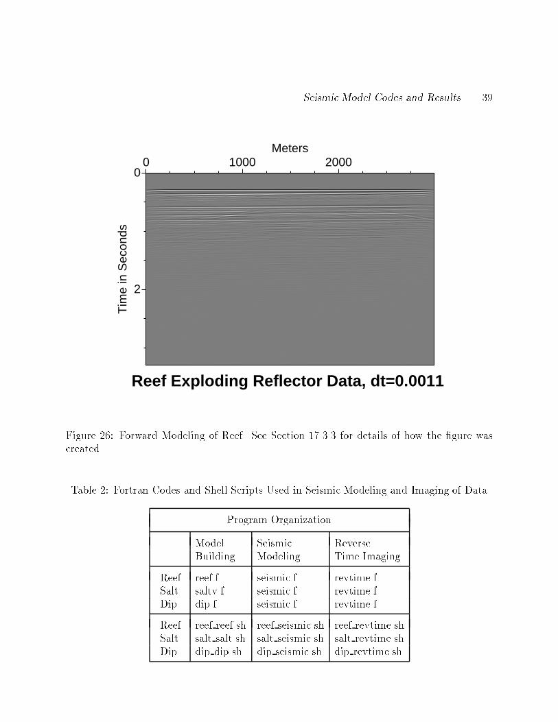
�� Reef Model Results

The reef model velocity �eld and exploding re�ector source locations are shown in Figures ��and �� respectively The computed model results are shown in Figures �� and �

The process by which the model was generated and the �gures created is described inthe next section

�� Model and Figure Generation

The Reef velocity model can be generated using the reef�f program and the model�dat �leThe user must specify the grid size� grid spacing� the length of time for the model run andthe time step A model name is also required

The output can be viewed with a postscript viewer such as ghostview A Unix shellprogram reef reef�sh is provided� and it generates a reef reef�ps �le The �rst process ofthe shell is to convert the unformatted output �le from reef�f into an SU format �le usingsuaddhead The shell uses SU program supsimage to convert the SU �le to postscript

The seismic image �le with the time data is generated using the seismic�f program Theoutput �le is processed by reef seismic�sh� which is a shell program that is similar to thereef reef�sh shell program It converts the program output into an SU �le and then into aps �le

The reverse time imaging which converts the time data back into depth data is gener�ated using the revtime�f program The output �le is processed by the reef revtime�sh shellsimilarly to reef reef�sh The depth image data �le is converted from a Fortran unformatted

��

0

1000

Dep

th in

Met

ers

0 1000 2000Meters

Reef Model, 200 by 300 grid

Figure �� Reef Model� Exploding Re�ector Source Locations See Section � �� for detailsof how the �gure was created

�le to an SU �le and then to a ps �leThe Salt Intrusion model and the Dipping layer models have Unix scripts and programs

identical to those for the Reef model The names of the �les used for all three models areshown in Table �

A comment about the shell programs described above they all require parameters tocreate output data images Any changes to model�dat will probably require changes in theshell programs

�� Salt Model

�� SALT Program

The salt program generates a velocity data �le for the seismic and revtime programs Someof the truly interesting geological structures are those made by salt and are typically foundin the Gulf of Mexico salt computes a salt body model� the principal feature is the highvelocity contrast between the salt and the surrounding geological media This particular saltmodel is an intrusion� a slowly moving feature pushing up and aside the inplace media� these


0

2

Tim

e in

Sec

onds

0 1000 2000Meters

Reef Exploding Reflector Data, dt=0.0011

Figure �� Forward Modeling of Reef See Section � �� for details of how the �gure wascreated

Table � Fortran Codes and Shell Scripts Used in Seismic Modeling and Imaging of Data

Program Organization

Model Seismic ReverseBuilding Modeling Time Imaging

Reef reeff seismicf revtimefSalt saltvf seismicf revtimefDip dipf seismicf revtimef

Reef reef reefsh reef seismicsh reef revtimeshSalt salt saltsh salt seismicsh salt revtimeshDip dip dipsh dip seismicsh dip revtimesh

��

0

500

1000

1500

Dep

th in

Met

ers

0 500 1000 1500 2000 2500Meters

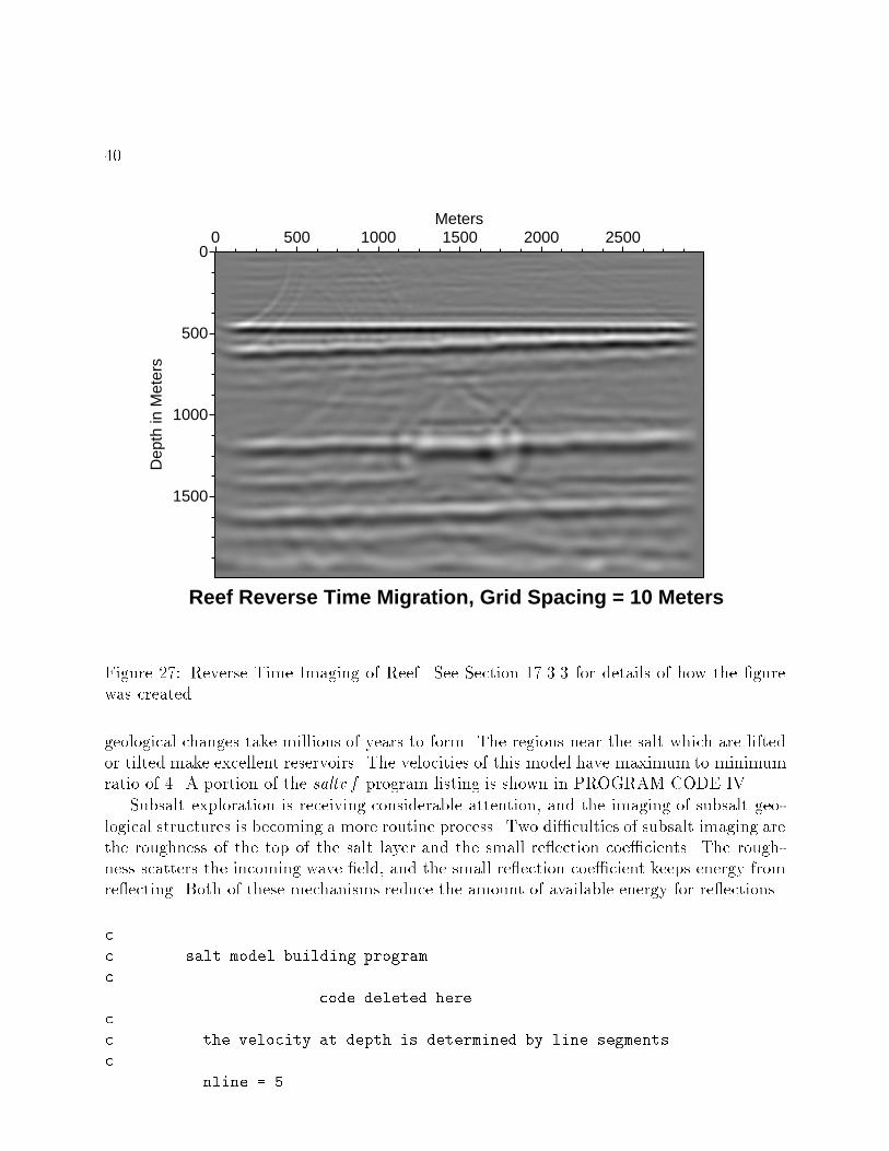
Reef Reverse Time Migration, Grid Spacing = 10 Meters

Figure � Reverse Time Imaging of Reef See Section � �� for details of how the �gurewas created

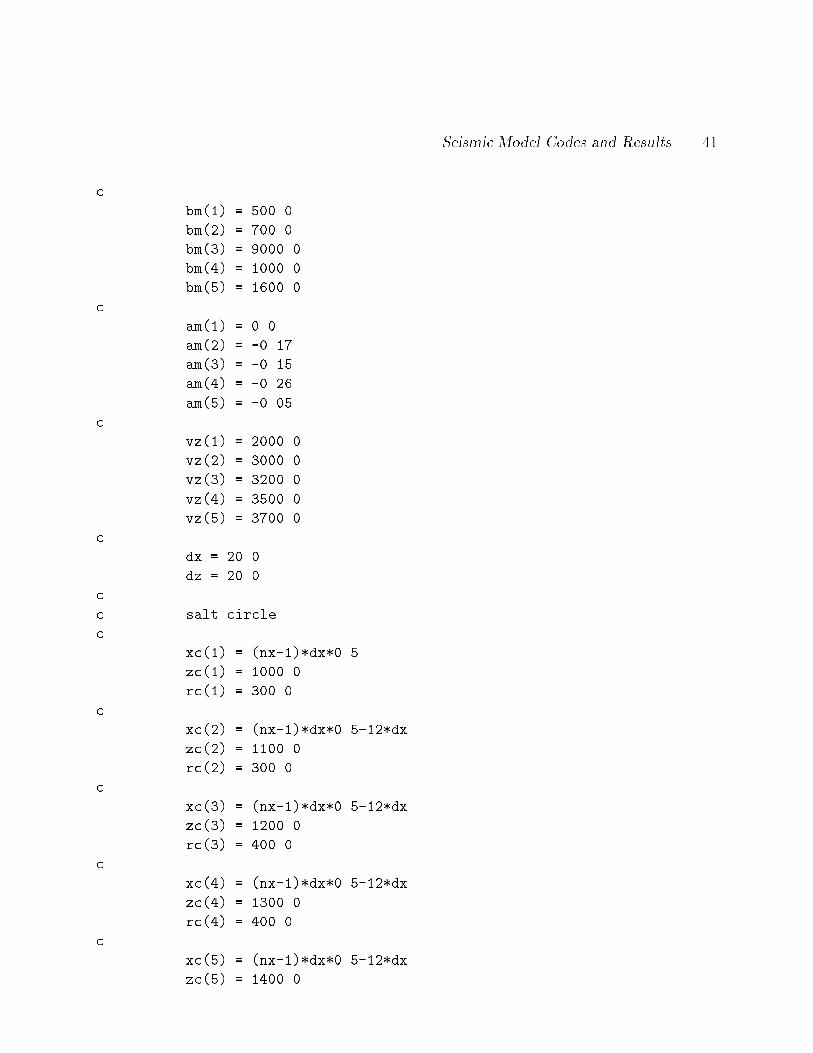
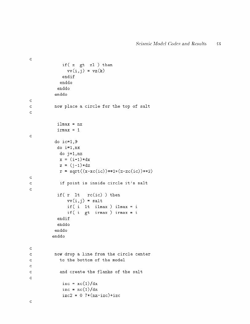
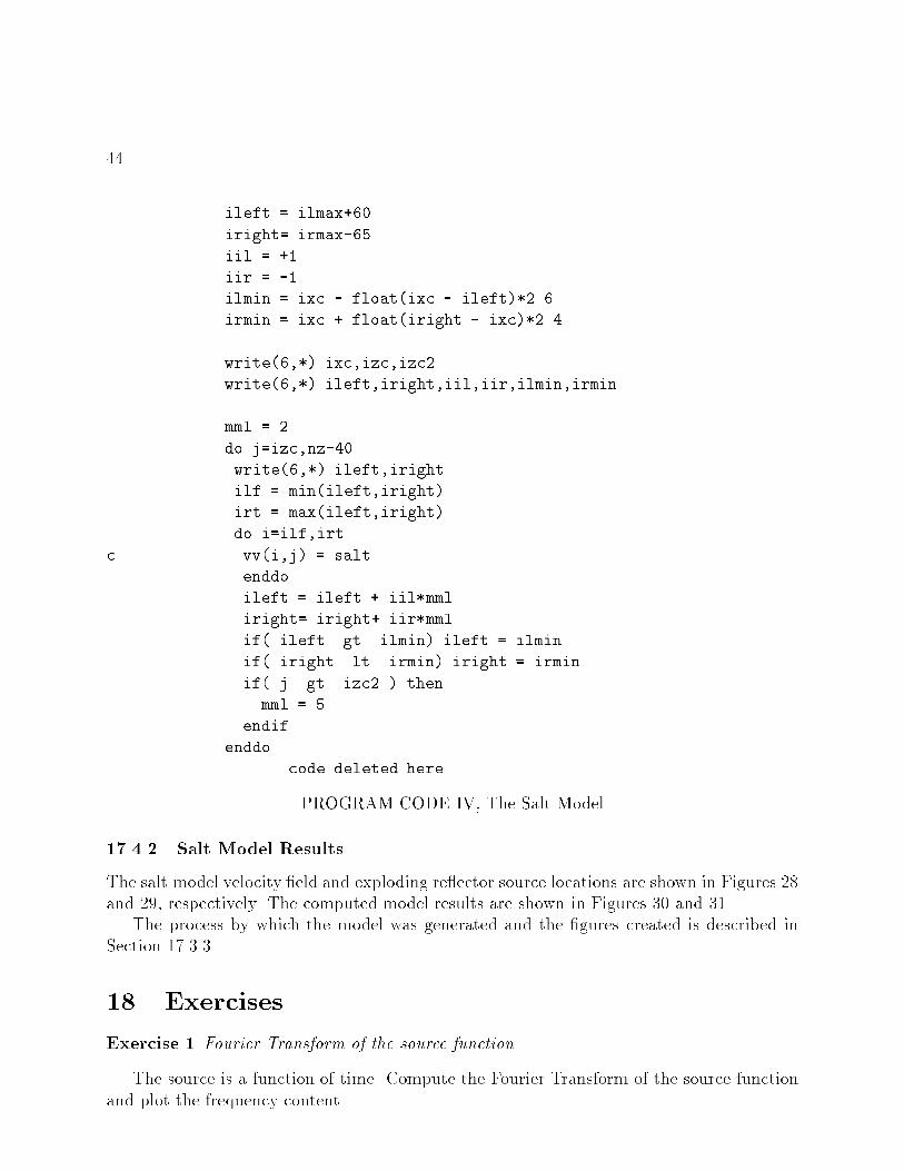
geological changes take millions of years to form The regions near the salt which are liftedor tilted make excellent reservoirs The velocities of this model have maximum to minimumratio of � A portion of the saltv�f program listing is shown in PROGRAM CODE IV

Subsalt exploration is receiving considerable attention� and the imaging of subsalt geo�logical structures is becoming a more routine process Two di�culties of subsalt imaging arethe roughness of the top of the salt layer and the small re�ection coe�cients The rough�ness scatters the incoming wave �eld� and the small re�ection coe�cient keeps energy fromre�ecting Both of these mechanisms reduce the amount of available energy for re�ections

c

c salt model building program

c


c


c

nline �


c

bm��

bm��

bm��

bm��

bm� � ��

c

am��

am��

am��

am��

am� � ��

c

vz��

vz��

vz��

vz��

vz� � ��

c

dx � ��

dz � ��

c

c salt circle

c

xc�� nx��dx��

zc��

rc��

c

xc�� nx��dx�� dx

zc��

rc��

c


zc��

rc��

c


zc��

rc��

c

xc� � �nx��dx�� dx

zc� � ��

��

rc� � ��

c


zc��

rc��

c


zc��

rc��

c


zc��

rc��

c


zc��

rc��

c

salt � � ��

c


c

do i��nx

do j��nz

vv�i�j � � ��


enddo

enddo

c


c line

c


c

do k��nline

sign � ��

do i��nx

if�i �gt� nx�� sign � ��

do j��nz

x � �i��dx

z � �j��dz

zl � sign�am�k�x bm�k


c


vv�i�j � vz�k

endif

enddo

enddo

enddo

c

c now place a circle for the top of salt

c

ilmax � nx

irmax � �

c

do ic��

do i��nx

do j��nz

x � �i��dx

z � �j��dz

r � sqrt��x�xc�ic��z�zc�ic��

c

c if point is inside circle it�s salt

c

if� r �lt� rc�ic then

vv�i�j � salt

if� i �lt� ilmax ilmax � i

if� i �gt� irmax irmax � i

endif

enddo

enddo

enddo

c

c now drop a line from the circle center

c to the bottom of the model

c

c and create the flanks of the salt

c

ixc � xc��dx

izc � zc��dz

izc� � ��nz�izcizc

c

��

ileft � ilmax��

iright� irmax��

iil � �

iir � ��

ilmin � ixc � float�ixc � ileft��

irmin � ixc float�iright � ixc��

write�� ixc�izc�izc�

write�� ileft�iright�iil�iir�ilmin�irmin

mml � �

do j�izc�nz��

write�� ileft�iright

ilf � min�ileft�iright

irt � max�ileft�iright

do i�ilf�irt

c vv�i�j � salt

enddo

ileft � ileft iil�mml

iright� iright iir�mml

if� ileft �gt� ilmin ileft � ilmin

if� iright �lt� irmin iright � irmin

if� j �gt� izc� then

mml �

endif

enddo


PROGRAM CODE IV� The Salt Model

�� Salt Model Results

The salt model velocity �eld and exploding re�ector source locations are shown in Figures ��and �� respectively The computed model results are shown in Figures �� and ��

The process by which the model was generated and the �gures created is described inSection � ��

�� Exercises

Exercise � Fourier Transform of the source function�

The source is a function of time Compute the Fourier Transform of the source functionand plot the frequency content

Exercises ��

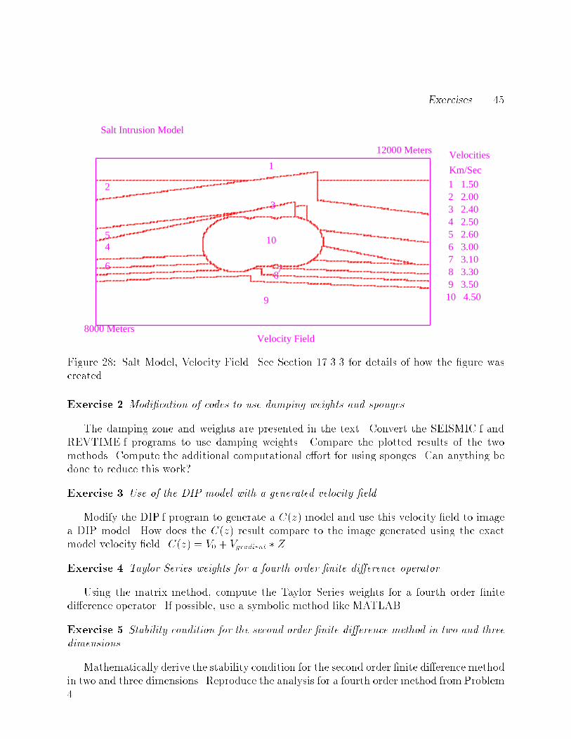
Velocity Field

Salt Intrusion Model

12000 Meters

8000 Meters

Velocities

Km/Sec

1 1.50

1

2 2.00 2

3 2.40 3

4 2.50

4 5 2.60 5 6 3.00

6 7 3.10

7 8 3.30 8 9 3.50

9 10 4.50

10

Figure �� Salt Model� Velocity Field See Section � �� for details of how the �gure wascreated

Exercise � Modi�cation of codes to use damping weights and sponges�

The damping zone and weights are presented in the text Convert the SEISMICf andREVTIMEf programs to use damping weights Compare the plotted results of the twomethods Compute the additional computational e�ort for using sponges Can anything bedone to reduce this work&

Exercise � Use of the DIP model with a generated velocity �eld�

Modify the DIPf program to generate a C�z� model and use this velocity �eld to imagea DIP model How does the C�z� result compare to the image generated using the exactmodel velocity �eld C�z� � V� � Vgradient � Z

Exercise � Taylor Series weights for a fourth order �nite di�erence operator�

Using the matrix method� compute the Taylor Series weights for a fourth order �nitedi�erence operator If possible� use a symbolic method like MATLAB

Exercise � Stability condition for the second order �nite di�erence method in two and three

dimensions�

Mathematically derive the stability condition for the second order �nite di�erence methodin two and three dimensions Reproduce the analysis for a fourth order method from Problem�

��

0

5000

Dep

th in

Met

ers

0 0.2 0.4 0.6 0.8 1.0x10 4Meters

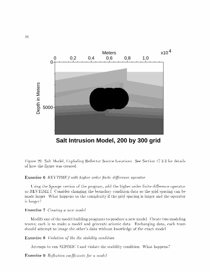
Salt Intrusion Model, 200 by 300 grid

Figure �� Salt Model� Exploding Re�ector Source Locations See Section � �� for detailsof how the �gure was created

Exercise � REVTIME�f with higher order �nite di�erence operator�

Using the Sponge version of the program� add the higher order �nite di�erence operatorto REVTIMEf Consider changing the boundary condition data so the grid spacing can bemade larger What happens to the complexity if the grid spacing is larger and the operatoris longer&

Exercise � Creating a new model�

Modify one of the model building programs to produce a new model Create two modelingteams� each is to make a model and generate seismic data Exchanging data� each teamshould attempt to image the other�s data without knowledge of the exact model

Exercise � Violation of the the stability condition�

Attempt to run SEISMICf and violate the stability condition What happens&

Exercise Re�ection coe�cients for a model�

Exercises �

0

2

Tim

e in

Sec

onds

0 0.2 0.4 0.6 0.8 1.0x10 4Meters

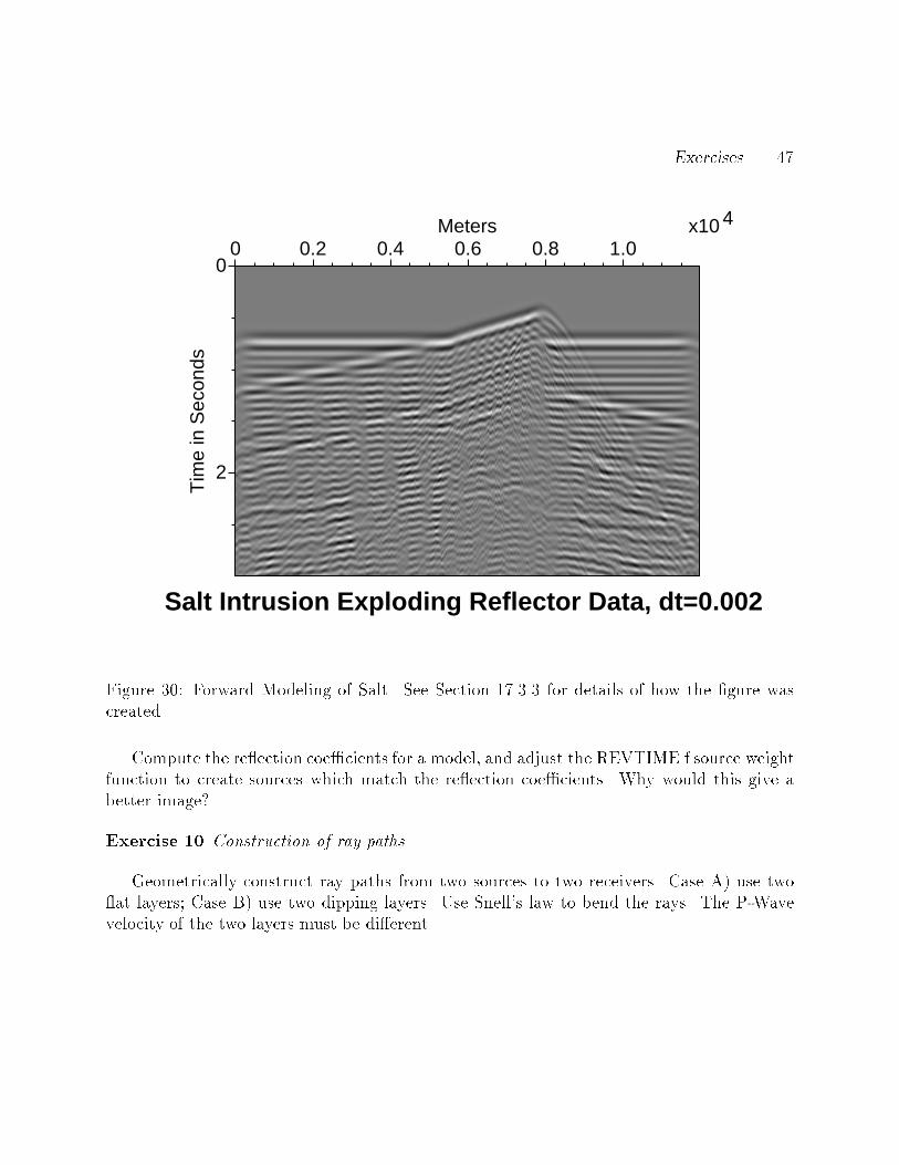
Salt Intrusion Exploding Reflector Data, dt=0.002

Figure �� Forward Modeling of Salt See Section � �� for details of how the �gure wascreated

Compute the re�ection coe�cients for a model� and adjust the REVTIMEf source weightfunction to create sources which match the re�ection coe�cients Why would this give abetter image&

Exercise � Construction of ray paths�

Geometrically construct ray paths from two sources to two receivers Case A� use two�at layers� Case B� use two dipping layers Use Snell�s law to bend the rays The P�Wavevelocity of the two layers must be di�erent

��

0

2000

4000

6000

Dep

th in

Met

ers

0 0.2 0.4 0.6 0.8 1.0x10 4Meters

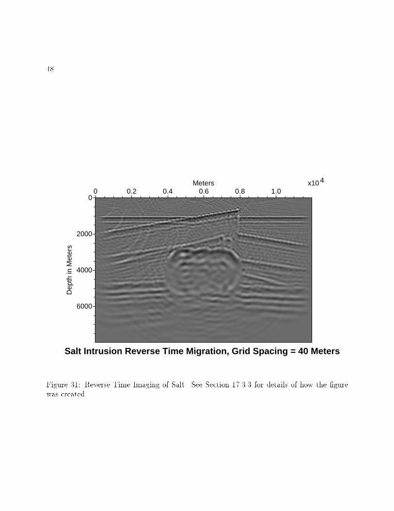
Salt Intrusion Reverse Time Migration, Grid Spacing = 40 Meters

Figure �� Reverse Time Imaging of Salt See Section � �� for details of how the �gurewas created

References ��

References

�� Aki� K� and Richards� P G� �� Quantitative Seismology� Volume I and II�W H Freeman and Co� New York

�� Alford� R M� Kelly� K R� and Boore� D M� �� Accuracy of Finite�

di�erence Modeling of the Acoustic Wave Equation� Geophysics� ��

�� Artley� J� �� Fields and Con�gurations� Holt� Rinehart� and Winston� Inc�New York

�� Cerjan� C� Koslo�� D� Koslo�� R� and Reshef� M� �� A Nonre�ecting

Boundary Condition for Discrete Acoustic and Elastic Wave Equations� Geo�physics� ��

�� Chew� W C� �� Waves and Fields in Inhomogeneous Media� Van NostrandReinhold� New York

�� Chung� T J� �� Finite Element Analysis in Fluid Dynamics� McGraw�Hill�New York

� Claerbout� J F� �� Fundamentals of Geophysical Data Processing� McGraw�Hill� New York

�� Claerbout� J F� �� Imaging the Earth�s Interior� Blackwell Scienti�c Publi�cations� Oxford� England

�� Clayton� R and Enquist� B� �� Absorbing Boundary Conditions for Acousticand Elastic Wave Equations� Bull Seis Soc Am� ��

�� Dablain� M A� �� The Application of High�Order Di�erencing to the Scalar

Wave Equation� Geophysics� ��

�� Hunter� S C� �� Mechanics of Continuous Media� Ellis Horwood� Sussex�England

�� Kelly� K R� Ward� R W� Treitel Sven� and Alford� R M� �� SyntheticSeismograms� A Finite Di�erence Approach� Geophysics� ��

�� Mufti� I R� �� Seismic Modeling in the Implicit Mode� Geophysical Prospect�ing� ��

�� Morse� P M and Feshbach� H� �� Methods of Theoretical Physics� McGraw�Hill Book Company� Inc� New York

�� Baker� L J� �� Supercomputers in Seismic Exploration� Pergamon Press�Oxford� ��

��

�� Mufti� I R� �� Supercomputers in Seismic Exploration� Pergamon Press�Oxford� ��

� � Oliger� J� �� Hybrid Di�erence Methods for the Initial Boundary�Value Prob�

lem for Hyperbolic Equations� Mathematics of Computation� Vol ��

�� Reynolds� A C� �� Boundary Conditions for the Numerical Solution of Wave

Propagation Problems� Geophysics� ��

�� Robinson� E A and Treitel� Sven� �� Geophysical Signal Analysis� PrenticeHall� Englewood Cli�s� New Jersey

�� Strikwerda� J C� �� Finite Di�erence Schemes and Partial Di�erential Equa�tions� Wadsworth ) Brooks"Cole� Belmont� Calif

�� Telford� W M� Geldart� L P� Sheri�� R E� and Keys� D A� �� AppliedGeophysics� Cambridge University Press� Cambridge

�� Weinberger� H F� A First Course in Partial Di�erential Equations� John Wileyand Sons� New York

Documents

Bording P. Seismic Wave Propagation, Modeling and Inversion (Comp. Science Education Project, 199