Embed Size (px)
Citation preview
Boosting Localized Features for Speaker and Speech Recognition
THESE No 5212 (2011)
PRESENTEE LE 6 OCTOBRE 2011
A LA FACULTE SCIENCES ET TECHNIQUES DE L’INGENIEUR
LABORATOIRE DE L’IDIAP
PROGRAMME DOCTORAL EN GENIE ELECTRIQUE
ECOLE POLYTECHNIQUE FEDERALE DE LAUSANNE
POUR L’OBTENTION DU GRADE DE DOCTEUR ES SCIENCES
PAR
Anindya Roy
acceptee sur proposition du jury :
Prof. Pierre Vandergheynst, president du jury
Prof. Herve Bourlard, directeur de these
Dr. Sebastien Marcel, co-directeur de these
Prof. Jan Cernocky, rapporteur
Dr. Nicholas Evans, rapporteur
Prof. Jean-Philippe Thiran, rapporteur
Lausanne, EPFL
2011

2

i
Abstract
In this thesis, we propose a novel approach for speaker and speech recognition involving local-
ized, binary, data-driven features. The proposed approach is largely inspired by similar localized
approaches in the computer vision domain. The success of these existing approaches coupled with
their proven advantages of robustness and computational efficiency motivated us to apply these
ideas to the speech domain. Our approach is distinct from the standard cepstral features-based
approach for speaker and speech recognition.
The proposed approach starts with a large set of simple localized features, each of which looks at
very small parts of spectro-temporal representations of speech. Each feature is binary-valued. The
most discriminative of these features are selected by boosting and combined to form the final clas-
sifier. Two systems are developed based on this general framework, a speaker recognition system
and a speech recognition system.
The speaker recognition system is evaluated under a wide range of experimental conditions,
using clean speech, noisy speech and speech data collected from mobile phones. The system per-
forms reliably in each condition, comparable with the standard systems using cepstral features
and Gaussian Mixture Models. At the same time, it involves significantly lower number of floating
point operations compared to these systems. In the case of the speech recognition system, we inte-
grate our localized features with a Hidden Markov Model framework using multilayer perceptrons.
Continuous speech recognition studies on standard databases show that these features perform
equally well as cepstral features. It is also found that the fusion of these features with cepstral
features leads to improved performance at both the feature level and the decision level.
Apart from this, minor contributions include an audio-visual person recognition system devel-
oped using the same general approach of localized features described above, extending its applica-
bility. Finally, a new (but related) class of localized features was developed for robust face detection.
Keywords : Speaker recognition, speech recognition, localized approach, boosting, noise-
robustness, computational complexity, audio-visual person recognition, face detection.
ii
Resume
Dans cette these, nous proposons une nouvelle methode pour la reconnaissance du locuteur et de
la parole, basee sur des primitives locales, binaires et selectionnees en fonction des donnees d’en-
traınement. Cette methode est inspiree des methodes locales du domaine de la vision par ordina-
teur. Le succes de ces methodes deja existantes, ainsi que leurs avantages demontres en termes de
robustesse et de rapidite nous ont motive a les appliquer au traitement de la parole. Notre methode
est distincte de la methode standard pour la reconnaissance du locuteur et de la parole basee sur
des coefficients cepstraux.
La methode proposee debute avec un grand ensemble de primitives locales, chacune d’entre elles
observant de petites parties des representations spectro-temporelles de la parole. Chaque primitive
a une valeur binaire. Les primitives les plus discriminatives sont selectionnees par boosting et com-
binees pour former le classifieur final. Bases sur cette methode, nous developpons deux systemes :
un pour la reconnaissance du locuteur, et un autre pour la reconnaissance de la parole.
Le systeme pour la reconnaissance du locuteur est evalue sous plusieurs conditions
experimentales, en utilisant un signal de parole sans bruit, un signal de parole avec bruit et un
signal de parole enregistre avec un telephone portable. Pour chacune de ces conditions, le systeme
fonctionne de facon fiable et comparable aux systemes standards qui utilisent des coefficients cep-
straux et des Modeles de Melange Gaussien. En outre, il requiert beaucoup moins d’operations en
virgule flottante. Pour la reconnaissance de la parole, nous integrons nos primitives locales avec un
Modele de Markov Cache utilisant des perceptrons multicouches. Les etudes relatives a la recon-
naissance de la parole continue sur les bases de donnes standards ont montre que les primitives
proposees fonctionnent aussi bien que les primitives a base de coefficients cepstraux. En outre,
la fusion de ces deux systemes aussi bien au niveau des primitives qu’au niveau de la decision a
engendre une amelioration des performances.
Les autres contributions mineures de cette these se constituent d’une methode de reconnais-
sance audio-visuelle des personnes et d’une classe de primitives locales pour la detection robuste de
visages.
Mots-cles : Reconnaissance du locuteur, reconnaissance de la parole, methode locale, boost-
ing, robustesse au bruit, complexite algorithmique, reconnaissance audio-visuelle des personnes,
detection de visages.
iii
Acknowledgements
Asato ma sad gamaya
Tamaso ma jyotir gamaya
Mrutyor ma amritam gamaya
From ignorance lead me to truth
From darkness lead me to light
From death lead me to immortality
- Brihadaranyaka Upanishad, 1.3.28
Doing this PhD was a joyful and exciting journey for me. There are several people who played
a critical role in this journey. Firstly, I should thank Sebastien for being the best supervisor a PhD
student could ever have. He was truly extraordinary: very methodical, resourceful and always ap-
preciative. He was ready to give his time whenever needed. In the same breath, I should thank
Mathew for being the best co-supervisor I could ever have. His contribution to this thesis is immea-
surable and cannot be expressed in words. I would also like to thank Herve, my thesis director, for
the fruitful discussions we had and his continued encouragement.
Then there are my friends who enriched every moment of my life and made me feel at home: Di-
nesh, Jagan, Marco, Gokul, Laurent, Deepu, Venky, Serena, Laxmi, Elie, Shruti, Stephanie, Jovana,
Tatiana, Flavio, Thomas, Anh-Thu, Minh, Valeria, Cyrielle, Ashtosh, Harsha, Sriram, Narges,
Cinzia, Cosmin, Afsaneh, Mohammad, Samira, Jakob, Tamara, Majid, Joel, Hari, Guillermo,
Hamed, Valerie, Chris, Paco, Niklas, Dayra, Alex, Marina, Joan, Marilu, Minh-Tri, Petr and so
many others. Thank you all. A special thanks to Francesco, who was always ready to discuss
aspects of machine learning and share his valuable insight.
I should also mention some of my colleagues at Idiap and EPFL who helped make my journey a
smooth one: Nadine, Sylvie, Corinne, Ed, Norbert, Frank, Bastien and all the system guys. Thank
you all.
Last but not the least, I should mention the contribution of my parents and grandparents. I
cannot thank them enough for all that they have done for me.

iv
Contents
1 Introduction 9
1.1 Objective of the thesis . . . . . . . . . . . . . . . . . . . . . . . . . . . . . . . . . . . . . 9
1.2 Motivations . . . . . . . . . . . . . . . . . . . . . . . . . . . . . . . . . . . . . . . . . . . . 10
1.3 Contributions . . . . . . . . . . . . . . . . . . . . . . . . . . . . . . . . . . . . . . . . . . 11
1.4 Organization . . . . . . . . . . . . . . . . . . . . . . . . . . . . . . . . . . . . . . . . . . . 14
2 Overview of the standard approach 15
2.1 Feature extraction . . . . . . . . . . . . . . . . . . . . . . . . . . . . . . . . . . . . . . . . 16
2.1.1 Mel Frequency Cepstral Coefficients . . . . . . . . . . . . . . . . . . . . . . . . . 17
2.1.2 Feature post-processing . . . . . . . . . . . . . . . . . . . . . . . . . . . . . . . . 19
2.2 Statistical modeling and Decision-making . . . . . . . . . . . . . . . . . . . . . . . . . . 20
2.2.1 Speaker recognition system . . . . . . . . . . . . . . . . . . . . . . . . . . . . . . 20
2.2.2 Speech recognition system . . . . . . . . . . . . . . . . . . . . . . . . . . . . . . . 23
2.3 Summary . . . . . . . . . . . . . . . . . . . . . . . . . . . . . . . . . . . . . . . . . . . . . 26
3 Preliminary idea of the proposed approach 27
3.1 A preliminary idea . . . . . . . . . . . . . . . . . . . . . . . . . . . . . . . . . . . . . . . 27
3.2 Localized approaches in computer vision . . . . . . . . . . . . . . . . . . . . . . . . . . . 28
3.2.1 Boosted Haar features . . . . . . . . . . . . . . . . . . . . . . . . . . . . . . . . . 28
3.2.2 Local Binary Patterns (LBP) . . . . . . . . . . . . . . . . . . . . . . . . . . . . . . 30
3.2.3 Fern features . . . . . . . . . . . . . . . . . . . . . . . . . . . . . . . . . . . . . . 32
3.3 Advantages and motivations . . . . . . . . . . . . . . . . . . . . . . . . . . . . . . . . . . 32
1

2 CONTENTS
3.4 Localized approaches in speech . . . . . . . . . . . . . . . . . . . . . . . . . . . . . . . . 33
3.4.1 Sub-band-based approach . . . . . . . . . . . . . . . . . . . . . . . . . . . . . . . 33
3.4.2 TempoRAl PatternS (TRAPS) . . . . . . . . . . . . . . . . . . . . . . . . . . . . . 33
3.4.3 Gabor features . . . . . . . . . . . . . . . . . . . . . . . . . . . . . . . . . . . . . . 34
3.4.4 Acoustic object detection . . . . . . . . . . . . . . . . . . . . . . . . . . . . . . . . 34
3.4.5 Parts-based models and local features . . . . . . . . . . . . . . . . . . . . . . . . 34
3.4.6 Boosted Haar features for music identification . . . . . . . . . . . . . . . . . . . 35
3.5 Summary . . . . . . . . . . . . . . . . . . . . . . . . . . . . . . . . . . . . . . . . . . . . . 35
4 The proposed approach 37
4.1 The proposed approach: Boosted Binary Features (BBF) . . . . . . . . . . . . . . . . . 37
4.2 Feature extraction . . . . . . . . . . . . . . . . . . . . . . . . . . . . . . . . . . . . . . . . 38
4.3 Modeling and decision-making . . . . . . . . . . . . . . . . . . . . . . . . . . . . . . . . 39
4.4 Feature Selection . . . . . . . . . . . . . . . . . . . . . . . . . . . . . . . . . . . . . . . . 40
4.5 Summary . . . . . . . . . . . . . . . . . . . . . . . . . . . . . . . . . . . . . . . . . . . . . 44
5 Application to Speaker Recognition 47
5.1 Objectives and motivations . . . . . . . . . . . . . . . . . . . . . . . . . . . . . . . . . . 47
5.2 Proposed BBF approach applied to speaker recognition . . . . . . . . . . . . . . . . . . 48
5.2.1 Feature extraction . . . . . . . . . . . . . . . . . . . . . . . . . . . . . . . . . . . 49
5.2.2 Modeling and Decision-making . . . . . . . . . . . . . . . . . . . . . . . . . . . . 50
5.3 Experimental validation - Brief overview . . . . . . . . . . . . . . . . . . . . . . . . . . 53
5.4 Group A Experiments . . . . . . . . . . . . . . . . . . . . . . . . . . . . . . . . . . . . . . 54
5.4.1 Experiments on clean speech: matched condition . . . . . . . . . . . . . . . . . . 54
5.4.2 Experiments on speech corrupted by additive noise: mismatched condition . . 59
5.4.3 Experiments on speech corrupted by channel noise: mismatched condition . . . 62
5.5 Group B Experiments . . . . . . . . . . . . . . . . . . . . . . . . . . . . . . . . . . . . . . 64
5.5.1 Database description . . . . . . . . . . . . . . . . . . . . . . . . . . . . . . . . . . 65
5.5.2 Systems evaluated . . . . . . . . . . . . . . . . . . . . . . . . . . . . . . . . . . . 66
5.5.3 Protocol and experimental details . . . . . . . . . . . . . . . . . . . . . . . . . . 67
5.5.4 Results . . . . . . . . . . . . . . . . . . . . . . . . . . . . . . . . . . . . . . . . . . 69
CONTENTS 3
5.6 Analysis of the proposed system applied to speaker recognition . . . . . . . . . . . . . 71
5.6.1 Robustness to additive noise . . . . . . . . . . . . . . . . . . . . . . . . . . . . . . 71
5.6.2 Complexity of the system . . . . . . . . . . . . . . . . . . . . . . . . . . . . . . . 75
5.6.3 Analysis of selected binary features . . . . . . . . . . . . . . . . . . . . . . . . . 77
5.7 Summary and concluding remarks . . . . . . . . . . . . . . . . . . . . . . . . . . . . . . 80
6 Application to Automatic Speech Recognition 83
6.1 Objectives and motivations . . . . . . . . . . . . . . . . . . . . . . . . . . . . . . . . . . 83
6.2 Proposed BBF approach applied to Automatic Speech Recognition (ASR) . . . . . . . . 84
6.2.1 Feature extraction: Boosted Binary Features . . . . . . . . . . . . . . . . . . . . 85
6.2.2 Modeling and decision-making . . . . . . . . . . . . . . . . . . . . . . . . . . . . 89
6.3 Experimental validation - A brief overview . . . . . . . . . . . . . . . . . . . . . . . . . 91
6.4 Group A experiments: Phoneme Recognition . . . . . . . . . . . . . . . . . . . . . . . . 92
6.4.1 Database description . . . . . . . . . . . . . . . . . . . . . . . . . . . . . . . . . . 92
6.4.2 Systems evaluated and experimental details . . . . . . . . . . . . . . . . . . . . 92
6.4.3 Results and discussions . . . . . . . . . . . . . . . . . . . . . . . . . . . . . . . . 95
6.5 Group B Experiments: Continuous Speech Recognition . . . . . . . . . . . . . . . . . . 97
6.5.1 Database description . . . . . . . . . . . . . . . . . . . . . . . . . . . . . . . . . . 97
6.5.2 Systems evaluated and experimental details . . . . . . . . . . . . . . . . . . . . 97
6.5.3 Results and Discussions . . . . . . . . . . . . . . . . . . . . . . . . . . . . . . . . 99
6.6 Group C Experiments: Fusion studies . . . . . . . . . . . . . . . . . . . . . . . . . . . . 101
6.6.1 Analysis of complementary nature of BBF and cepstral features . . . . . . . . . 101
6.6.2 Fusion experiments . . . . . . . . . . . . . . . . . . . . . . . . . . . . . . . . . . . 103
6.6.3 Results and discussions . . . . . . . . . . . . . . . . . . . . . . . . . . . . . . . . 103
6.7 Summary and concluding remarks . . . . . . . . . . . . . . . . . . . . . . . . . . . . . . 104
7 Conclusions and future work 107
7.1 Application to speaker recognition . . . . . . . . . . . . . . . . . . . . . . . . . . . . . . 107
7.2 Application to speech recognition . . . . . . . . . . . . . . . . . . . . . . . . . . . . . . . 109
7.3 General directions for future work . . . . . . . . . . . . . . . . . . . . . . . . . . . . . . 111
4 CONTENTS
Appendices 115
A Localized Audio-Visual features 115
A.1 The Proposed Framework . . . . . . . . . . . . . . . . . . . . . . . . . . . . . . . . . . . 116
A.1.1 Localized Audio-visual features: Slice classifiers . . . . . . . . . . . . . . . . . . 116
A.1.2 Slice Classifier Selection and Combination by Boosting . . . . . . . . . . . . . . 117
A.2 Experiments . . . . . . . . . . . . . . . . . . . . . . . . . . . . . . . . . . . . . . . . . . . 118
A.2.1 Database and Protocol . . . . . . . . . . . . . . . . . . . . . . . . . . . . . . . . . 118
A.2.2 Systems implemented . . . . . . . . . . . . . . . . . . . . . . . . . . . . . . . . . 119
A.2.3 Results . . . . . . . . . . . . . . . . . . . . . . . . . . . . . . . . . . . . . . . . . . 120
A.3 Discussions . . . . . . . . . . . . . . . . . . . . . . . . . . . . . . . . . . . . . . . . . . . . 120
A.3.1 Speaker Verification Performance . . . . . . . . . . . . . . . . . . . . . . . . . . . 120
A.3.2 Computational Complexity . . . . . . . . . . . . . . . . . . . . . . . . . . . . . . 121
A.4 Conclusions . . . . . . . . . . . . . . . . . . . . . . . . . . . . . . . . . . . . . . . . . . . 121
B HLBP features for Face Detection 125
B.1 The Proposed Framework : Face Detection using HLBP features . . . . . . . . . . . . 127
B.1.1 General Boosting Framework . . . . . . . . . . . . . . . . . . . . . . . . . . . . . 127
B.1.2 The proposed HLBP features . . . . . . . . . . . . . . . . . . . . . . . . . . . . . 128
B.1.3 Advantage of HLBP features over Haar features . . . . . . . . . . . . . . . . . . 131
B.2 Experiments . . . . . . . . . . . . . . . . . . . . . . . . . . . . . . . . . . . . . . . . . . . 132
B.2.1 Reference systems and databases used . . . . . . . . . . . . . . . . . . . . . . . . 132
B.2.2 Results and discussions . . . . . . . . . . . . . . . . . . . . . . . . . . . . . . . . 133
B.3 Conclusions . . . . . . . . . . . . . . . . . . . . . . . . . . . . . . . . . . . . . . . . . . . 136
Curriculum Vitae 149
List of Figures
2.1 Simplified structure of a standard speaker or speech recognition system. . . . . . . . . 16
2.2 Simplified structure of a standard cepstral feature extraction module. . . . . . . . . . 19
3.1 The five types of masks used for the calculation of Haar features, I. Bihorizontal, II.
Bivertical, III. Diagonal, IV. Trihorizontal, V. Trivertical. . . . . . . . . . . . . . . . . . 29
3.2 The first and second features selected by AdaBoost for face detection . . . . . . . . . . 30
3.3 Computation of LBP . . . . . . . . . . . . . . . . . . . . . . . . . . . . . . . . . . . . . . 31
3.4 Robustness of LBP to monotonic gray-scale transformations . . . . . . . . . . . . . . . 32
4.1 An example binary feature . . . . . . . . . . . . . . . . . . . . . . . . . . . . . . . . . . . 39
4.2 Histogram of the binary features based on their misclassification error on training
data for a typical client class in a speaker recognition task. . . . . . . . . . . . . . . . . 41
5.1 Client and impostor distributions of the spectral differences corresponding to the first
two binary features selected by Adaboost . . . . . . . . . . . . . . . . . . . . . . . . . . 51
5.2 Variation of training error with the number of binary features used . . . . . . . . . . . 53
5.3 Equal Error Rates (EER %) for same-sex (M only, F only) and mixed-sex (F+M) exper-
iments on the TIMIT database . . . . . . . . . . . . . . . . . . . . . . . . . . . . . . . . 58
5.4 Equal Error Rates (EER %) for mixed-sex (F+M) experiments on the noisy TIMIT
database . . . . . . . . . . . . . . . . . . . . . . . . . . . . . . . . . . . . . . . . . . . . . 61
5.5 Equal Error Rates (EER %) for mixed-sex (F+M) experiments on the HTIMIT database 64
5.6 Distribution of utterances in the MOBIO Phase I database, according to (a) their SNR
(dB), (b) amount of speech in seconds. . . . . . . . . . . . . . . . . . . . . . . . . . . . . 66
5
6 LIST OF FIGURES
5.7 Half Total Error Rates (HTER %) for SV experiments on the Test set of the MOBIO
Phase I database. . . . . . . . . . . . . . . . . . . . . . . . . . . . . . . . . . . . . . . . . 70
5.8 Effect of additive noise on the proposed binary features and MFCC features . . . . . . 73
5.9 Number of floating-point operations, NFLOP plotted in log-scale, for 17 reference sys-
tems and the proposed BBF system. . . . . . . . . . . . . . . . . . . . . . . . . . . . . . 77
5.10 Distribution of binary feature weights selected by Adaboost . . . . . . . . . . . . . . . 79
5.11 Distributions of k and |∆k| associated with the binary features selected by Adaboost. 80
6.1 An example binary feature for ASR . . . . . . . . . . . . . . . . . . . . . . . . . . . . . . 86
6.2 Time-frequency bin pairs of the first 8 boosted features for phonemes /eh/, /ah/, /p/
and /s/ shown on the spectro-temporal matrix. . . . . . . . . . . . . . . . . . . . . . . . 88
6.3 A Kullback Leibler divergence-based Hidden Markov Model system . . . . . . . . . . . 90
B.1 Robustness of LBP to monotonic gray-scale transformations . . . . . . . . . . . . . . . 127
B.2 Calculation of LBP . . . . . . . . . . . . . . . . . . . . . . . . . . . . . . . . . . . . . . . 128
B.3 The five types of masks used for the calculation of both Haar and HLBP features, I.
Bihorizontal, II. Bivertical, III. Diagonal, IV. Trihorizontal, V. Trivertical. . . . . . . . 129
B.4 Calculation of the sum of LBP label counts within region R using Integral Histogram
(ref. Eqn. B.10). . . . . . . . . . . . . . . . . . . . . . . . . . . . . . . . . . . . . . . . . . 130
B.5 Calculation of HLBP features . . . . . . . . . . . . . . . . . . . . . . . . . . . . . . . . . 130
B.6 Comparison of face detection performance on different datasets by the three systems
using Haar, HLBP and MCT features: (a) XM2VTS Normal set, (b) XM2VTS Dark-
ened set, (c) BioID database and (d) Fleuret database. . . . . . . . . . . . . . . . . . . . 134
List of Tables
3.1 Contrasting aspects of the standard and proposed approaches. . . . . . . . . . . . . . . 28
5.1 Basic parameters of the reference systems, grouped according to submitting institution. 68
6.1 Number of input units for SLP and MLP, and number of hidden units for MLP. . . . . 95
6.2 Frame accuracy on cross validation (CV) set and phoneme recognition rate on test set
of the TIMIT database expressed in %. . . . . . . . . . . . . . . . . . . . . . . . . . . . . 96
6.3 Frame-level phoneme accuracy (%) on RM development set. . . . . . . . . . . . . . . . 99
6.4 Word Error Rate (%) on evaluation set of RM database using context-independent and
context-dependent sub-word unit based systems. . . . . . . . . . . . . . . . . . . . . . . 100
6.5 Distribution (%) of frames from cross-validation set of TIMIT database on the basis
of performance of MFCC and BBF. . . . . . . . . . . . . . . . . . . . . . . . . . . . . . . 102
6.6 Best feature and relative improvement in frame accuracy on cross-validation set of
TIMIT database for a subset of phonemes. . . . . . . . . . . . . . . . . . . . . . . . . . . 102
6.7 Results of different systems using MFCC, BBF and fusion of the two (in %). . . . . . . 104
A.1 Verification performance of the Boosted Slice Classifier systems . . . . . . . . . . . . . 122
A.2 Comparison of verification performance of Boosted Slice Classifier systems with ref-
erence systems . . . . . . . . . . . . . . . . . . . . . . . . . . . . . . . . . . . . . . . . . . 123
B.1 Description of the databases used in our experiments . . . . . . . . . . . . . . . . . . . 133
B.2 Comparison of storage requirements (in bits) and the number of free parameters per
feature of the 3 systems, Haar, HLBP and MCT . . . . . . . . . . . . . . . . . . . . . . 135
7

8 LIST OF TABLES
Chapter 1
Introduction
Automatic speaker and speech recognition systems have been under active research since a few
decades. The task of an automatic speaker recognition system is to recognize a person, based on
acoustic (speech) data recorded from that person and stored in digital form. The task of an auto-
matic speech recognition system is to decode the acoustic data recorded from a person in terms of
the actual sequence of words that the person intended to convey. Today, progress in technology has
enabled such automatic systems implemented on computers and portable devices such as smart-
phones to perform these functions reliably under certain conditions. This thesis is yet another small
step in this direction.
1.1 Objective of the thesis
In the standard approach for automatic speaker and speech recognition, the recorded speech
waveform is converted into a sequence of cepstral features. These cepstral features look at the
entire short-term magnitude spectrum of speech as a whole. Hence, they could be termed as holis-
tic. 1 Furthermore, they are real-valued and motivated by prior knowledge about the human speech
perception and production systems. Once extracted, these features are typically modeled using
Gaussian Mixture Models (GMM).
The objective of this thesis is to propose a different approach for speaker and speech recognition.
1. The holistic nature of cepstral features is justified more clearly in later chapters.
9
10 CHAPTER 1. INTRODUCTION
The fundamental idea behind this approach is to use a novel set of localized, discrete-valued fea-
tures selected in a data-driven way with more emphasis on machine learning and less emphasis on
prior knowledge. By “localized”, it is signified that each such feature looks at a localized region or
part of the short-term speech spectrum instead of the entire spectrum. Hence, this approach may
also be called “parts-based”.
1.2 Motivations
The approach proposed in this thesis is inspired by and based on similar existing approaches in
the computer vision domain which have shown considerable success in recent years.
Examples of such approaches in the vision domain include Local Binary Patterns (LBP), an
image texture descriptor introduced by Ojala et al. in 1996, the face detection algorithm proposed
by Viola and Jones in 2001 using a boosted cascade of Haar features and the Fern features-based
keypoint detection algorithm proposed by Ozuysal et al. in 2010. A significant amount of research
has been carried out in developing and extending these approaches (particularly the first two) and
successfully applying them to a wide range of tasks. The proposed approach draws ideas from all
these approaches.
The success of these approaches in the vision domain is mainly due to two chief advantages: 1)
robustness in uncontrolled illumination conditions, and 2) a simple framework with low computa-
tional complexity. These positive aspects are the chief motivations of this thesis. It is hypothesized
that these advantages will be carried over to the speech domain by the proposed approach.
In particular, it is hypothesized that robustness to illumination conditions in the vision domain
would be transformed to robustness to noise in the speech domain. In fact, there is prior work in
the speech domain in this direction which supports this hypothesis. Examples of existing localized
approaches in the speech domain include the sub-band based approach by Bourlard et al., the
TRAPS system by Hermansky et al. and the local features and parts-based models by Schutte et
al. All these systems are robust to noise.
Hence, localized approaches also exist in the speech domain. However, only few of these ap-
proaches (e.g. the one by Schutte et al.) are directly inspired by localized approaches in the vision
domain. This thesis is an effort to bridge this gap between vision and speech research by introduc-
1.3. CONTRIBUTIONS 11
ing more speech researchers to a promising approach from the vision domain.
1.3 Contributions
The contributions of this thesis are as follows.
1. We proposed a generic localized approach to solve pattern recognition problems in
the speech domain. The fundamental idea of this approach is to convert the speech wave-
form into a sequence of spectro-temporal segments. The difference in magnitude at two par-
ticular time-frequency bins in such a spectro-temporal segment is compared with a threshold.
The corresponding feature is assigned a discrete (binary) value of 1 or -1 depending on the
result of this comparison. Every pair of time-frequency bins corresponds to a feature. This
leads to a very large set of features. Out of these, the most discriminative features relevant
to the task are selected in a data-driven way using the Discrete Adaboost algorithm. These
features are called Boosted Binary Features (BBF).
Note that the approach is generic: it could be applied to any speech pattern classification
problem as long as the relevant class labels are specified. For example, the labels could be
client or impostor in the case of speaker recognition, and the different phonemes in the case of
speech recognition. 2
2. We applied the proposed approach to the task of text-independent speaker recogni-
tion (Roy et al., 2011a,c). A very simple system was developed for this purpose. In this
system, the boosted binary features are combined via a linear weighted summation function.
To our knowledge, this is the first time that such an approach has been applied to this task.
A point to note here is that speaker recognition could mean either speaker verification or
speaker identification. 3 In this thesis, we have chosen to deal with the speaker verification
task only. 4 Hence, the term “speaker recognition” always means “speaker verification” and
the two terms are used interchangeably.
2. The phonemes are the basic units of sound considered in automatic speech recognition systems.3. In the speaker verification task, a person claims to be a particular speaker (the client) and the system has to verify
this claim based on his or her voice, i.e. it has to decide if the person is the client or an impostor. On the other hand, in thespeaker identification task, a speaker is identified as one person from among a set of possible persons.
4. This task is associated with applications such as access control, e-banking and phone banking, and is related to one ofthe main projects under which this work was carried out, i.e. the Mobile Biometry (MOBIO) project (www.mobioproject.org).
12 CHAPTER 1. INTRODUCTION
We evaluated the performance of the proposed system through multiple speaker recognition
experiments using several databases. The performance of the proposed system was compared
with that of standard cepstral features-based systems. These experiments can be grouped as
follows:
(a) Experiments on clean speech: In these experiments, the systems were trained and
tested using clean speech. The proposed system performed reasonably and equally well
as the standard systems.
(b) Experiments on noisy speech: In these experiments, the systems were trained using
clean speech but tested using noisy speech. Different types of additive and convolutive
noises were considered. In this case, the proposed system often outperformed the stan-
dard systems. This illustrates the noise-robust characteristic of the proposed system
hypothesized before.
(c) Experiments on speech collected from mobile phones: In these experiments, the
systems were trained using speech recorded using mobile phones in a realistic scenario.
Again, the performance of the proposed system was reasonable and compared well with
the standard systems.
In addition to these experiments, the computational complexity of the proposed speaker recog-
nition system was analysed and compared with that of the standard ones. It was found that
the proposed system was about 102 times faster than the standard systems. This illustrated
another positive aspect of the proposed approach in addition to robustness to noise: a simple
framework with low computational complexity. Note that this advantage is also exhibited by
localized systems in the vision domain.
3. Motivated by the good performance of the proposed approach in speaker recognition, we ap-
plied it to the task of automatic speech recognition (Roy et al., 2011b,d).
In this case, the proposed approach was used as a feature extractor: the Adaboost algorithm
was used to select localized binary features which were most useful in discriminating individ-
ual phonemes against all other phonemes. The selected binary features were then integrated
into a standard Hidden Markov Model-based automatic speech recognition system by model-
ing them by single layer perceptrons and multilayer perceptrons.
1.3. CONTRIBUTIONS 13
The performance of the proposed approach was evaluated on a phoneme recognition task and
a continuous speech recognition task. The proposed features performed equally well as the
standard cepstral features on these tasks. It was found that the proposed features were more
amenable to simpler modeling frameworks like single layer perceptrons than the standard
features. Furthermore, it was found that the proposed features selected using a particular
database could generalize well to unseen data.
Due to their contrasting nature, it was hypothesized that the proposed features and standard
features could contain useful complementary information. Hence, a speech recognition system
was created by fusion of the proposed features with the standard features. Two cases were
investigated: 1) fusion at the feature level and 2) fusion at the decision level. In both the cases,
it was found that fusion of the two features led to improved phoneme recognition performance.
This showed that the proposed approach could be advantageously combined with the standard
approach.
4. Apart from these primary contributions, there are some secondary contributions of this thesis
which are related in some way to the main work. These are as follows.
Firstly, we proposed a similar localized approach for audio-visual person recognition,
involving feature-level fusion of audio and video modalities (Roy and Marcel, 2010b). The
proposed system was evaluated on a standard audio-visual database under two experimental
conditions: a) matched-clean: Here, original clean data from the database was used for both
training and testing. b) Mismatched-noisy: Here, the training data was clean, but the audio
modality of the test data was corrupted by additive noise.
The proposed system was comparedwith standard unimodal (only audio and only video-based)
systems and bimodal score-level fusion systems. Experimental results showed that the pro-
posed system is robust to noisy acoustic environments and compares well with score-level
fusion.
Secondly, we proposed a new visual feature called Haar Local Binary Pattern (HLBP) for
face-detection which combines the concepts of Haar feature and Local Binary Patterns in a
compact way (Roy and Marcel, 2009). Note that our main contribution in the speech domain
was also inspired by such ideas from the computer vision domain.
We designed a face detection system using such features selected and combined using Ad-
14 CHAPTER 1. INTRODUCTION
aboost. Our system performs significantly better in adverse imaging conditions than usual
Haar features and performs reasonably better than Modified Census Transform (MCT) fea-
tures, a standard approach, with much less storage and computation requirements.
1.4 Organization
The structure of this thesis is as follows.
– Chapter 2 provides a brief overview of the standard approaches to speaker and speech recog-
nition. The purpose of this chapter is to provide a context and contrast with the proposed
approach which will be introduced in subsequent chapters.
– Chapter 3 provides a preliminary idea of the proposed approach and a brief overview of similar
approaches from speech and computer vision domains. These existing successful approaches
are cited in order to motivate the proposed approach.
– Chapter 4 describes the proposed approach in details. However, the description in this chapter
is at a generic level. No specific task (speaker or speech recognition) is considered in this
chapter.
– Chapter 5 describes the application of the proposed approach to the task of speaker recogni-
tion. Experimental studies on a wide range of databases and under different experimental
conditions are reported. The proposed approach is compared with the standard approach, and
several aspects of the proposed approach is discussed. This includes robustness to noise and
computational complexity.
– Chapter 6 describes the application of the proposed approach to the task of speech recognition.
Several experimental studies are reported, including phoneme recognition, continuous word
recognition and a fusion of the proposed and standard approaches.
– Chapter 7 concludes the thesis with a brief summary of the important contributions made and
outlining the potential directions for future work.
– In the Appendix, we describe some of the secondary contributions of this thesis. These include
the work on Haar Local Binary Patterns and the work on localized features for audio-visual
person recognition.
Chapter 2
Overview of the standard
approach for speaker and speech
recognition
In this chapter, we briefly describe the main building blocks of standard speaker and speech
recognition systems. In fact, it is difficult to select one speaker or speech recognition system as
the “standard” one. A large number of different approaches have been proposed and implemented.
However, a majority of them could be seen as variations or extensions of the basic approach de-
scribed here.
Speaker or speech recognition systems aim to predict the correct class Ω∗ corresponding to an
observation O, from among a set of classes Ω. The observation O is a spoken utterance. In the
case of speaker recognition, the classes Ω denote speakers (Bimbot et al., 2004). In the case of
speech recognition, they denote sequences of words (Gales and Young, 2007). The system predicts
the class Ω∗ which maximizes the posterior probability of the class, conditioned on the observation
O (Duda et al., 2000), i.e.,
Ω∗ = argmaxΩ
P(Ω|O) (2.1)
15
16 CHAPTER 2. OVERVIEW OF THE STANDARD APPROACH
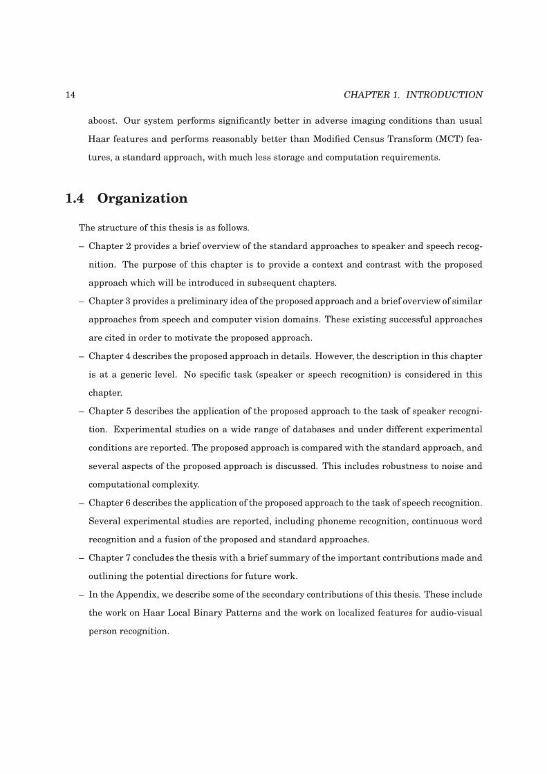
Figure 2.1. Simplified structure of a standard speaker or speech recognition system. The arrows signify the direction ofthe flow of information. Please consult the text for details.
Note that in the case of speech recognition, each class is actually a sequence of words. This requires
a more complex search strategy compared to speaker recognition which often comprises of only two
speaker classes: the client (true) speaker and the impostor. 1 To implement Equation 2.1 above,
three basic modules are necessary (Duda et al., 2000). They are as follows:
1. Feature extraction to convert the observation O to a more suitable form,
2. Statistical modeling to estimate the posterior probability function P, and
3. Decision-making to implement the max operation in a suitable way.
Figure 2.1 shows a simplified structure of a speaker or speech recognition system with these three
modules. Note that the flow of information is always in one direction: from the feature extraction
module to the modeling module and then the decision-making module. There is no information
flowing back from the modeling module to the extraction module. A description of each of these
modules follows.
2.1 Feature extraction
The input to this module is the raw observation obtained from a spoken utterance, i.e. a speech
waveform typically sampled at 16 KHz (microphone speech) or 8 KHz (telephone speech). The
entire waveform is first blocked into analysis frames of about 20 ms. Each frame of speech is then
converted into another representation, which: 1) maximizes the information relevant to the task
(speaker or speech recognition), 2) reduces dimensionality, and 3) makes the new representation
more suitable for the subsequent statistical modelingmodule (Bimbot et al., 2004; Gales and Young,
1. This is strictly true only for speaker verification and not speaker recognition which can involve more than two classes.However, even speaker recognition does not consider sequences of any form as speech recognition does.
2.1. FEATURE EXTRACTION 17
2007). This conversion is termed as feature extraction and the output of this module is a sequence
of feature vectors. This module is often identical in both speaker and speech recognition systems,
although task-specific modifications do exist.
Typically, the first objective of maximizing relevant information is indirectly addressed by using
prior knowledge of the human auditory perception and speech production systems. The assump-
tion here is that a system which is able to mimic the human system would be an efficient one, since
humans are good at the same tasks, i.e. speaker and speech recognition. This prior knowledge is es-
sentially represented as different ways of obtaining a smoothed envelope of the short-time spectrum
of speech. Depending on the type of prior knowledge and smoothing strategy used, two different
sets of feature vectors could be extracted: 1) Mel Frequency Cepstral Coefficients (MFCC) (Davies
and Mermelstein, 1980) or 2) Perceptual Linear Prediction (PLP) Cepstral Coefficients (Herman-
sky, 1990). The former uses prior knowledge of the human auditory perception system while the
latter uses knowledge of both the speech perception and production systems. The extraction of one
of these features, i.e. MFCC, is described next.
2.1.1 Mel Frequency Cepstral Coefficients
The extraction of MFCC involves the following steps:
1. Framing, windowing, DFT: The speech waveform is blocked into frames of size ranging
from 20 to 25 ms with a shift of 10 ms. Next, a short-time Discrete Fourier Transform (DFT)
is applied to each frame and only the magnitude is retained. This conversion to the frequency
domain is motivated by the frequency-dependent response of the human cochlea (Steinberg,
1937). The DFT is just the fastest way to get such a frequency representation.
2. Mel filterbank: Although we have a frequency representation now, it could be improved. For
this, prior knowledge of the human auditory perception system is used. It has been found
that the perception of audio in humans follows a nonlinear frequency scale termed the Mel
scale (Davies and Mermelstein, 1980). This scale is obtained by warping the linear frequency
h in Hz to a logarithmic frequencym expressed in units called Mels as follows:
m (Mel) = 2595 · log10(1 +h (Hz)
700) (2.2)
18 CHAPTER 2. OVERVIEW OF THE STANDARD APPROACH
This knowledge is incorporated into the feature extraction stage by applying a bank of trian-
gular filters spaced according to the Mel frequency scale to the Fourier magnitude spectra.
The number of filters is typically around 20 to 30. The energy under each filter is summed
to form a set of Mel frequency spectral coefficients collectively called the Mel spectrum. Note
that this stage effectively leads to a smoothing of the spectrum.
3. Logarithm: Further knowledge of the human perceptual system is included by taking the
logarithm of the Mel spectral coefficients (Davies and Mermelstein, 1980). This leads to a
compression of the dynamic range.
4. DCT: For each frame, a Discrete Cosine Transform (DCT) is applied to the log Mel frequency
coefficients and the first NDCT DCT coefficients are kept (typical values of NDCT range from 12
to 16). 2 This helps to decorrelate the features required for the subsequent statistical modeling
stage, reduce dimensionality and further smoothen the spectral profile. The final output is a
set of coefficients called the Mel Frequency Cepstral Coefficients (MFCC).
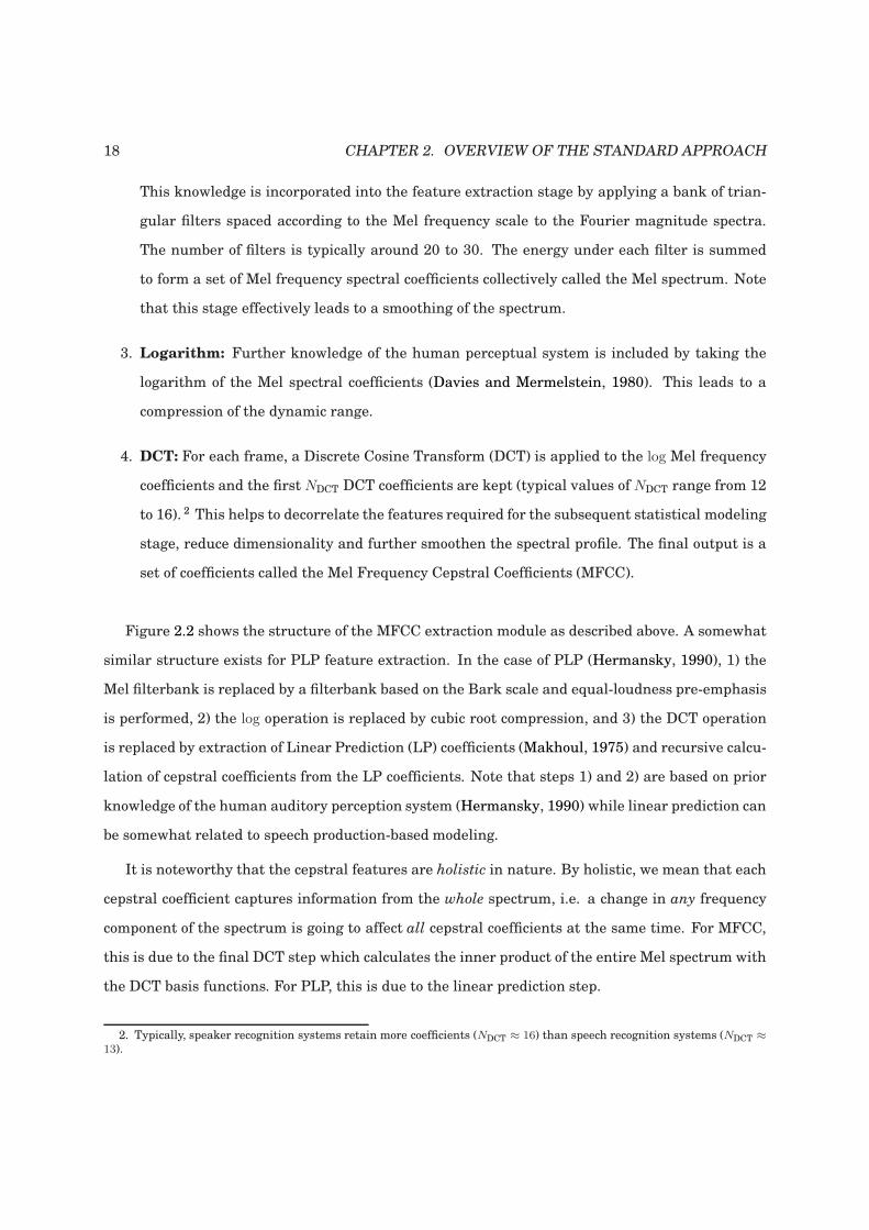
Figure 2.2 shows the structure of the MFCC extraction module as described above. A somewhat
similar structure exists for PLP feature extraction. In the case of PLP (Hermansky, 1990), 1) the
Mel filterbank is replaced by a filterbank based on the Bark scale and equal-loudness pre-emphasis
is performed, 2) the log operation is replaced by cubic root compression, and 3) the DCT operation
is replaced by extraction of Linear Prediction (LP) coefficients (Makhoul, 1975) and recursive calcu-
lation of cepstral coefficients from the LP coefficients. Note that steps 1) and 2) are based on prior
knowledge of the human auditory perception system (Hermansky, 1990) while linear prediction can
be somewhat related to speech production-based modeling.
It is noteworthy that the cepstral features are holistic in nature. By holistic, we mean that each
cepstral coefficient captures information from the whole spectrum, i.e. a change in any frequency
component of the spectrum is going to affect all cepstral coefficients at the same time. For MFCC,
this is due to the final DCT step which calculates the inner product of the entire Mel spectrum with
the DCT basis functions. For PLP, this is due to the linear prediction step.
2. Typically, speaker recognition systems retain more coefficients (NDCT ≈ 16) than speech recognition systems (NDCT ≈13).
2.1. FEATURE EXTRACTION 19
Figure 2.2. Simplified structure of a standard cepstral feature extraction module. Please consult the text for details.
2.1.2 Feature post-processing
Several post-processing steps could be applied to further improve the feature vector representa-
tion.
1. Mean and variance normalization: The mean feature vector estimated over an entire
utterance is subtracted from each MFCC vector (Bimbot et al., 2004). This helps reduce the
sensitivity to convolutive noise, provided they do not vary significantly over the utterance.
Variance normalization scales each feature to have unit variance; empirically, this has been
found to reduce the sensitivity to additive noise (Hain et al., 1999).
2. Addition of dynamic information: Once the MFCC feature vectors cm have been calcu-
lated, their first and second order temporal derivatives are estimated as follows:
∆cm =
∑Ncon
k=−Nconk · cm+k
∑Ncon
k=−Ncon|k|
, (2.3)
∆∆cm =
∑Ncon
k=−Nconk ·∆cm+k
∑Ncon
k=−Ncon|k|
. (2.4)
where Ncon denotes the number of frames before and after the reference frame that are used
for the computation, i.e. the temporal context. This adds useful dynamic information relating
to how the feature vectors vary in time (Furui, 1986; Bimbot et al., 2004).
3. Silence frames are not useful. Hence, feature vectors corresponding to the silence frames are
discarded. This is typically done by modeling the features using a bi-Gaussian distribution
and discarding those vectors which have a higher likelihood with the Gaussian having the
lower energy (Bimbot et al., 2004).
4. Other post-processing steps include Gaussianization, Vocal Tract Length Normalization
(VTLN) and linear projections like Principal Component Analysis (PCA), Linear Discriminant

20 CHAPTER 2. OVERVIEW OF THE STANDARD APPROACH
Analysis (LDA), Maximum Likelihood Linear Regression (MLLR), etc.
The sequence of feature vectors extracted in this module are modelled statistically to capture class-
specific characteristics in the next module. This is described in the following section.
2.2 Statistical modeling and Decision-making
As mentioned earlier, a speaker or speech recognition system predicts the class (speaker or
word sequence)Ω∗ which maximizes the posterior probability, given the observationO (Duda et al.,
2000), as stated in Equation 2.1. The purpose of the statistical modeling stage is to estimate the
posterior probability function P(Ω|O) in this equation. The Bayes’ Theorem (Duda et al., 2000) is
used to restate Equation 2.1 in a more tractable form as follows:
Ω∗ = argmaxΩ
P(Ω|O)
= argmaxΩ
p(O|Ω)P(Ω)
p(O)
(using the Bayes’ Theorem)
≡ argmaxΩ
p(O|Ω)P(Ω)
≡ argmaxΩ
log p(O|Ω) + logP(Ω) (2.5)
Hence, the problem is broken into two parts, estimating 1) the likelihood p(O|Ω), and 2) the prior
P(Ω). Since these are approached in slightly different ways in speaker and speech recognition sys-
tems, separate descriptions of these modules for each of these systems is provided in the following
subsections.
2.2.1 Speaker recognition system
The statistical modeling module in a speaker recognition system is implemented as follows.
The likelihood function p(O|Ω) in Equation 2.5 is typically modeled using Gaussian Mixture Mod-
els (GMM) (Reynolds and Rose, 1995; Gales and Young, 2007). Note that as a result of feature
extraction, the observation O is now represented as a sequence of feature vectors. Let us denote
this sequence as: O ≡ o1, · · · ,oNO. Then, the likelihood p(ot|Ω) of a single feature vector ot is
2.2. STATISTICAL MODELING AND DECISION-MAKING 21
expressed as a weighted linear combination of NG component densities as follows:
p(ot|Ω) =
NG∑
g=1
w(g)Ω
p(g)Ω
(ot) (2.6)
where w(g)ΩNG
g=1 are the component weights and each component p(g)Ω
is a unimodal Gaussian den-
sity with mean µ(g)Ω
and covariance matrix Σ(g)Ω
:
p(g)Ω
(ot) = N (ot;µ(g)Ω
,Σ(g)Ω
) (2.7)
Note that the component weights w(g)ΩNG
g=1 should be positive and sum to unity. The parameters
of the model for the class Ω is represented collectively as: λΩ ≡ w(g)Ω
, µ(g)Ω
,Σ(g)ΩNG
g=1. Often, only
diagonal covariance matrices are used (Bimbot et al., 2004; Gales and Young, 2007) in order to
robustly estimate the parameters using limited amount of training data.
The model parameters are estimated as follows. All the feature vectors extracted from a large
pool of speakers called the background set or world set is modelled by a single GMM whose param-
eters are estimated via the Expectation-Maximization (EM) algorithm (Bimbot et al., 2004). Note
that this set excludes all client speakers. This single speaker-independentGMM usually has a large
number of Gaussians (NG ≈ 2000) and is called the Universal Background Model (UBM).
Each new client speaker is then modelled by Maximum a posteriori (MAP) adaptation (of often
only the means) of this UBM using the feature vectors extracted from this client, yielding the client-
specific GMM (Gauvain and Lee, 1994). Though less common nowadays, client-specific GMMs could
also be trained individually using Maximum-Likelihood (ML) training on only client-specific data.
Assuming independent feature vectors, the log-likelihood log p(O|Ω) in Equation 2.5 correspond-
ing to an utterance observation O ≡ o1, · · · ,ot, · · · ,oNO is computed as:
log p(O|Ω) =1
NO
NO∑
t=1
log p(ot|Ω) (2.8)
where p(ot|Ω) is calculated via Equation 2.6. Note that the prior term P(Ω) in Equation 2.5 is not
determined directly. Rather, it is accounted for in terms of a detection threshold in the decision-
making module (Bimbot et al., 2004). This completes the basic statistical modeling module for a
22 CHAPTER 2. OVERVIEW OF THE STANDARD APPROACH
speaker recognition system. Here, we described a generative approach for modeling the classes.
This is currently one of the most popular and efficient approaches (Bimbot et al., 2004). Alterna-
tive discriminative approaches using Artificial Neural Networks (ANN) also exist (Bennani and
Gallinari, 1995).
In the decision-making module of a speaker recognition system, 3 the classes to be predicted
are: 1) the client (true) speaker, and 2) the impostor. The latter represents all speakers other than
the client. Let ΩC and ΩI represent these two classes respectively. Firstly, the log-likelihood ratio
(LLR), i.e. the ratio of logarithms of the two likelihoods coming from the client and impostor classes,
is calculated as follows:
LLR = log p(O|ΩC)− log p(O|ΩI) (2.9)
The two likelihoods in the above equation are calculated using Equation 2.8. Then the class is
predicted by restating Equation 2.5 as:
Ω∗ =
ΩC (predict client) if LLR ≥ Θ,
ΩI (predict impostor) otherwise.
(2.10)
where Θ is a threshold that effectively accounts for the prior term in Equation 2.5. This represents
a simple hypothesis-testing scenario (Bimbot et al., 2004).
Typically, the UBM is considered as representing the impostor class (Bimbot et al., 2004). In an-
other approach less common nowadays, sets of speakers termed as cohorts are individually selected
for each client to act as the impostors for estimating p(O|ΩI) (Bimbot et al., 2004; Reynolds, 1995).
The threshold Θ is selected a priori using separate development data (often called validation data)
not used in training. This completes the basic decision-making module for a speaker recognition
system.
The above description corresponds to a basic or baseline speaker recognition system. A state-of-
the-art system often involves further levels of sophistication:
1. In the modeling module, the mean vectors of the adapted GMMs may be concatenated to
form a GMM supervector. This supervector may be considered as an utterance-level feature
3. more specifically, a speaker verification system.
2.2. STATISTICAL MODELING AND DECISION-MAKING 23
vector and modeled using a Support Vector Machine (SVM) classifier with different types of
kernels (Campbell et al., 2006).
Alternative approaches such as Latent Factor Analysis (LFA) (Matrouf et al., 2007), Joint Fac-
tor Analysis (JFA) (Kenny et al., 2007) and the I-vector system (Dehak et al., 2009) decompose
the space of GMM supervectors into eigendirections that represent speaker and channel vari-
abilities. This is an effective method of compensating for inter-session variability, one of the
main problems arising in speaker verification systems.
2. The decision-making module may involve score normalization techniques like Z-norm, H-
norm, T-norm, etc. (Bimbot et al., 2004).
2.2.2 Speech recognition system
The statistical modeling module in a speech recognition system is implemented as follows.
Let us rewrite Equation 2.5 again:
Ω∗ = argmaxΩ
P(Ω|O)
= argmaxΩ
p(O|Ω)P(Ω)
p(O)
≡ argmaxΩ
p(O|Ω)P(Ω) (2.11)
In the case of speech recognition, the likelihood p(O|Ω) is determined by an acousticmodel and the
prior P(Ω) is determined by a language model (Gales and Young, 2007). The observation O is an
ordered sequence of feature vectors O ≡ o1, · · · ,oNO.
Any class Ω in a speech recognition system is a sequence of words. Typically, this sequence
is first converted into an equivalent sequence of basic units of sound called phones according to
a pronunciation dictionary. For example, the sequence of words “the bat” is converted into the
equivalent sequence of phones: /dh/ /ix/ /b/ /ae/ /t/.
To account for the temporal variability in speech (i.e. the fact that the same sound is not always
uttered with the same time duration), the phones are represented by left-to-right Hidden Markov
Models (HMM) which assume that the vectors have been generated by a Markov process with
unobserved (hidden) states (Rabiner, 1989). The composite acoustic model for class Ω is formed
by concatenating these HMM states s ≡ s1, · · · , st, · · · , sNO aggregated over all the phones in the

24 CHAPTER 2. OVERVIEW OF THE STANDARD APPROACH
sequence in the right order, each state st emitting a feature vector ot. Note that multiple state
sequences are possible for the same phone sequence.
Given a sequence of feature vectors O ≡ o1, · · · ,ot, · · · ,oNO and a state sequence s ≡
s1, · · · , st, · · · , sNO through the composite model, the acoustic likelihood is calculated as:
p(O|Ω) ≡∑
s
p(O|s) =∑
s
as0s1
NO∏
t=1
bst(ot)astst+1 (2.12)
where aij denotes the transition probability from state i to state j for any two states i and j, bj(ot)
is the emission likelihood of the feature vector ot given state j, i.e. bj(ot) ≡ p(ot|j), and s0 and
sNOare the non-emitting entry and exit states. Note that the summation is over all possible state
sequences s corresponding to Ω.
The state emission likelihoods bj are typically modeled by a GMM:
bj(ot) ≡ p(ot|j) =NG∑
g=1
w(g)j p
(g)j (ot) (2.13)
where p(g)j (ot) = N (ot;µ
(g)j ,Σ
(g)j ) is a unimodal Gaussian density. The parameters of the GMM,
i.e. the means µ(g)j and covariance matrices Σ
(g)j , and the transition probabilities aij are
estimated using a modified form of the EM algorithm, the Baum-Welch Forward-Backward algo-
rithm (Gales and Young, 2007; Rabiner, 1989).
As an alternative to GMMs which represent a generative approach, the states can also be mod-
eled discriminatively using Artificial Neural Networks (ANN), particularly Multilayer Perceptrons
(MLP) (Bourlard and Morgan, 1994); such systems are called hybrid systems. Both types of ap-
proaches have shown equally good performance.
As mentioned before, the prior probability P(Ω) in Equation 2.5 is determined by a language
model which is an N -gram model (Gales and Young, 2007). Let the class Ω represent the sequence
of Nw words w1, · · · , wNw. Then, the prior probability is given by:
P(Ω) ≡ P(w1, · · · , wNw) =
Nw∏
k=1
P(wk|wk−1, wk−2, · · · , wk−N+1) (2.14)
where N typically ranges from 2 to 4. The probabilities P(wk|wk−1, wk−2, · · · , wk−N+1) are esti-
2.2. STATISTICAL MODELING AND DECISION-MAKING 25
mated separately from text data. This model represents the language-specific syntactic constraints
for different words to follow each other in a particular utterance. This completes the basic statistical
modeling module of a speech recognition system.
Note that a practical system usually has some additional stages, such as context-dependent
modeling of phones and tying of the context-dependent models (Gales and Young, 2007). Also re-
cently, a different form of HMM has been proposed: the Kullback-Leibler divergence-based Hidden
Markov Model (KL-HMM) (Aradilla et al., 2008). In this model, the posterior probabilities of the
phoneme classes are used directly as feature observations. The KL-HMM based system will be
discussed further in Chapter 6.
In the decision-making module, the word sequence (i.e. class Ω∗) that is most likely to have
generated the sequence of extracted feature vectorsO ≡ o1, · · · ,oNO is found by searching over all
possible state sequences corresponding to all possible word sequences, and finding the one which
maximizes the posterior probability in Equation 2.5. This process is called decoding (Gales and
Young, 2007).
An efficient way to perform decoding is by using dynamic programming. Let φ(j)t denote the
maximum probability of observing the partial sequence O1:t ≡ o1, · · · ,ot and being at state j at
time t. The initial value φ(j)0 is set to 1. Then, subsequent values φ
(j)t t=1,··· ,NO
can be efficiently
computed using the Viterbi algorithm (Viterbi, 1967):
φ(j)t = max
iφ
(i)t−1aijbj(ot) (2.15)
where aij and bj denote the transition probabilities and state emission likelihoods respectively,
as described earlier. Then, the probability of the most likely word sequence Ω∗ to have generated
O is given by maxjφ(j)NO. The most likely word sequence is then found by a traceback through the
maximization decision in Equation 2.15 from t = NO back to t = 1.
This completes the basic decision-making module for a speech recognition system. Note that
modifications and additions to this basic structure such as stack decoders or word lattices often
exist in practical implementations of such a system (Gales and Young, 2007).
26 CHAPTER 2. OVERVIEW OF THE STANDARD APPROACH
2.3 Summary
In this chapter, we described the standard approach for speaker and speech recognition. This
approach uses cepstral features typically modeled by Gaussian Mixture Models. In the case of
speech recognition, Hidden Markov Models are used for sequence modeling. Before we end this
chapter, let us summarize certain aspects of the standard approach:
1. The approach is holistic. This characteristic is not only present in the cepstral features (ref.
Section 2.1) but it is also shared by the GMMs in the modeling module. This is because the
GMMs look at all the cepstral features as a whole (i.e. the entire feature vector) and not a
subset of them.
2. The features are based on prior knowledge of the human speech perception and production
systems (Hermansky, 1990; Davies and Mermelstein, 1980; Fletcher, 1953).
3. The features are real-valued (continuous).
4. The feature extraction module and the modeling module work independently, i.e. the model-
ing module does not provide any feedback information to the feature extraction module (for
example, to facilitate feature selection). 4
4. In fact, this is related to the first point: the system is holistic. Hence, there is no feature selection; the feature vectoras a whole is used.
Chapter 3
Preliminary idea of the proposed
approach and overview of similar
existing approaches
In this chapter, we provide a preliminary idea of the proposed approach for speaker and speech
recognition by listing some of the main characteristics of this approach. Then we present a brief
overview of existing approaches in the computer vision domain which inspired the proposed ap-
proach. The advantages of these approaches are highlighted in order to motivate the proposed ap-
proach. This is followed by a short description of existing approaches in the speech domain which
share some characteristics with the proposed approach.
3.1 A preliminary idea
This thesis proposes a novel approach for speaker and speech recognition. The approach is
characterized by the following aspects:
1. The approaches uses features which are localized or parts-based. More precisely, each
feature looks at a small region or part of spectro-temporal segments of speech.
2. The approach gives relatively less emphasis on prior knowledge; rather, it gives more empha-
27
28 CHAPTER 3. PRELIMINARY IDEA OF THE PROPOSED APPROACH
sis on data-driven learning and selection of features.
3. The features used are binary-valued (quantized).
4. The feature extraction and modeling modules are strongly linked. Features are selected de-
pending on how well they perform in the modeling module.
These aspects contrast with those of the standard approach listed in the last chapter. For conve-
nience, Table 3.1 provides a brief summary of this contrast.
Standard approach Proposed approach
Holistic Localized
More emphasis on prior knowledge More emphasis on data-driven learning
Continuous, real-valued features Binary-valued features
No feedback link from modeling to Feedback link from modeling to
feature extraction feature extraction via feature selection
Table 3.1. Contrasting aspects of the standard and proposed approaches.
3.2 Localized approaches in computer vision
Asmentioned in Chapter 1, the proposed approach draws ideas from a group of approaches in the
computer vision domain which share some of the characteristics with the proposed approach, par-
ticularly the localized nature of the features. In this section, we review these existing approaches
in the vision domain.
3.2.1 Boosted Haar features
Originally described in (Viola and Jones, 2001), this approach has emerged as one of the mile-
stones in the computer vision community for the face detection task (Rodriguez, 2006). This ap-
proach places rectangular masks (similar to Haar wavelets) at different locations and scales in the
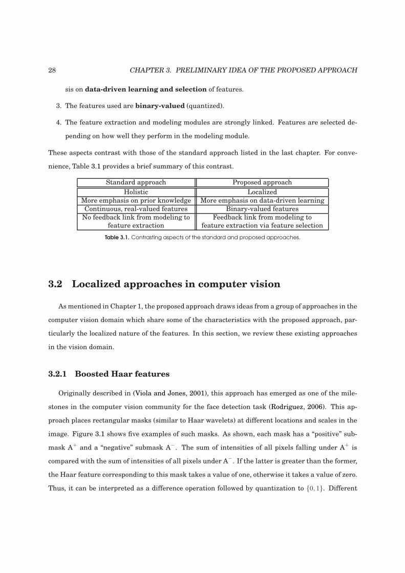
image. Figure 3.1 shows five examples of such masks. As shown, each mask has a “positive” sub-
mask A+
and a “negative” submask A−. The sum of intensities of all pixels falling under A
+is
compared with the sum of intensities of all pixels under A−. If the latter is greater than the former,
the Haar feature corresponding to this mask takes a value of one, otherwise it takes a value of zero.
Thus, it can be interpreted as a difference operation followed by quantization to 0, 1. Different
3.2. LOCALIZED APPROACHES IN COMPUTER VISION 29
types, locations and scales of the masks lead to different Haar features. In this way, a very large
number of Haar features are created.
Figure 3.1. The five types of masks used for the calculation of Haar features, I. Bihorizontal, II. Bivertical, III. Diagonal, IV.Trihorizontal, V. Trivertical.
A feature selection algorithm based on the Discrete Adaboost algorithm (Friedman et al., 1998)
is then used to select the most discriminative of these features, i.e. those features which can
discriminate best between face and non-face. 1 The final face detector (face/non-face classifier) is
formed by a simple linear weighted sum of the selected features. There exists various modifica-
tions and enhancements of the original feature set and the boosting algorithm used (please refer
to (Rodriguez, 2006) for details).
This approach has all the characteristics mentioned before: it uses localized, data-driven, bi-
nary 0, 1 features. The feature selection based on Adaboost provides a feedback link between the
modeling and feature extraction modules. Some aspects of this approach are as follows (Viola and
Jones, 2001):
1. The approach is efficient (Rodriguez, 2006). This approach and its subsequent improvements
have remained one of the best performing approaches for face detection since its inception.
2. The approach is very fast, capable of real-time performance. Operating on 384 by 288 pixel
images, the approach ran at 15 frames per second on a 700 MHz Intel Pentium III (Viola and
Jones, 2001). The number of computations is vastly reduced compared to previous approaches.
This is due to 1) the simple features (based on summation and comparison only) 2 and, 2) the
simple linear sum-based modeling module.
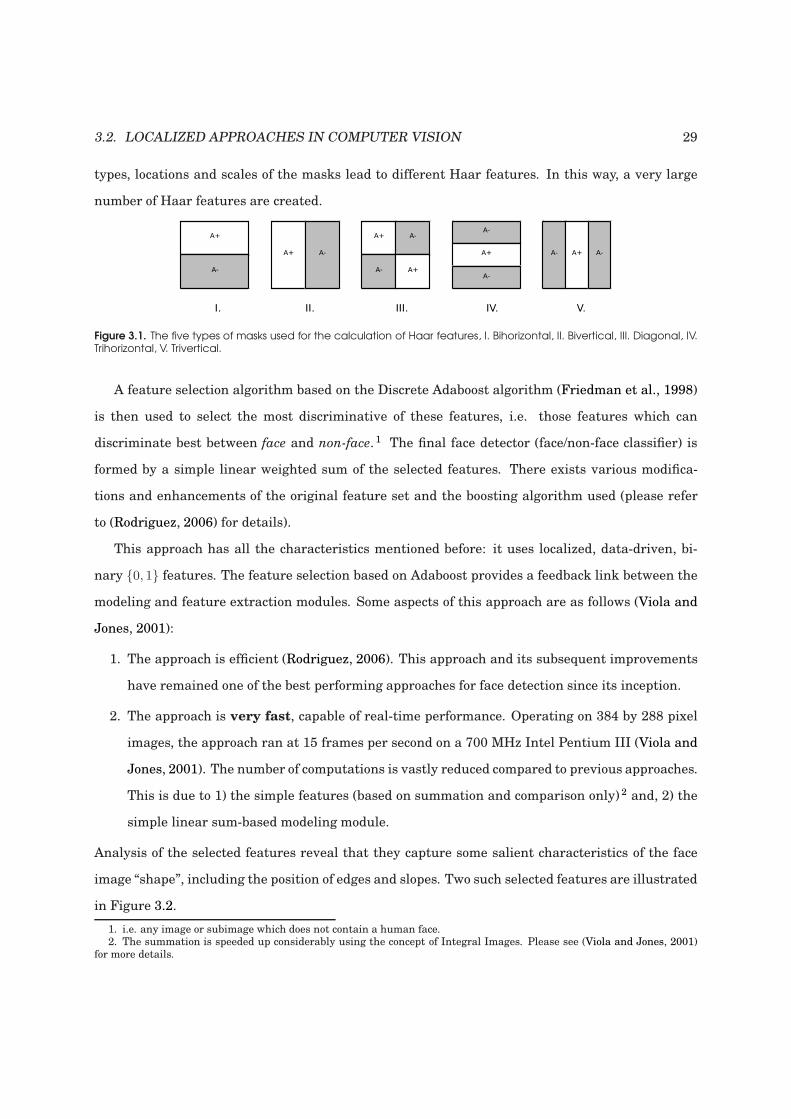
Analysis of the selected features reveal that they capture some salient characteristics of the face
image “shape”, including the position of edges and slopes. Two such selected features are illustrated
in Figure 3.2.
1. i.e. any image or subimage which does not contain a human face.2. The summation is speeded up considerably using the concept of Integral Images. Please see (Viola and Jones, 2001)
for more details.
30 CHAPTER 3. PRELIMINARY IDEA OF THE PROPOSED APPROACH
Figure 3.2. The first and second features selected by AdaBoost for face detection (courtesy of (Viola and Jones, 2001)).The two features are shown in the top row and then overlayed on a typical face image in the bottom row. The firstfeature measures seems to capture the information that the eye region is often darker than the cheeks. The secondseems to capture the fact that the eye regions are often darker than the bridge of the nose.
3.2.2 Local Binary Patterns (LBP)
This approach was first proposed in (Ojala et al., 1996) as a localized descriptor of image texture.
It has remained one of the most widely-used approaches in computer vision with numerous appli-
cations including face and object detection and face verification (Rodriguez, 2006; Heusch et al.,
2006).
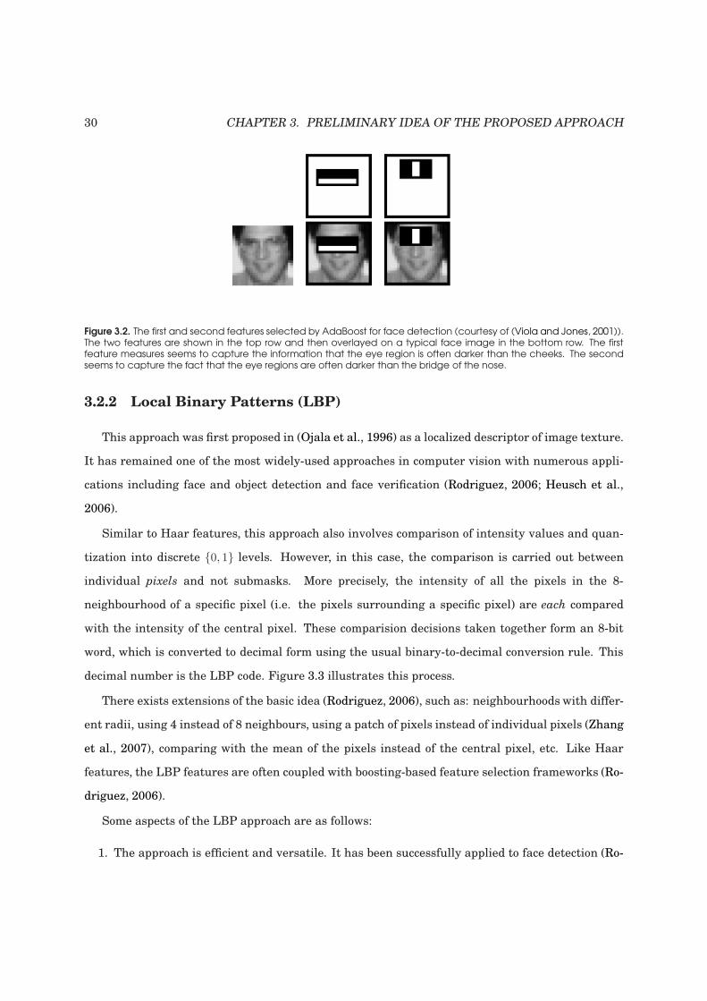
Similar to Haar features, this approach also involves comparison of intensity values and quan-
tization into discrete 0, 1 levels. However, in this case, the comparison is carried out between
individual pixels and not submasks. More precisely, the intensity of all the pixels in the 8-
neighbourhood of a specific pixel (i.e. the pixels surrounding a specific pixel) are each compared
with the intensity of the central pixel. These comparision decisions taken together form an 8-bit
word, which is converted to decimal form using the usual binary-to-decimal conversion rule. This
decimal number is the LBP code. Figure 3.3 illustrates this process.
There exists extensions of the basic idea (Rodriguez, 2006), such as: neighbourhoods with differ-
ent radii, using 4 instead of 8 neighbours, using a patch of pixels instead of individual pixels (Zhang
et al., 2007), comparing with the mean of the pixels instead of the central pixel, etc. Like Haar
features, the LBP features are often coupled with boosting-based feature selection frameworks (Ro-
driguez, 2006).
Some aspects of the LBP approach are as follows:
1. The approach is efficient and versatile. It has been successfully applied to face detection (Ro-
3.2. LOCALIZED APPROACHES IN COMPUTER VISION 31
Figure 3.3. LBP computation (courtesy www.cse.oulu.fi): In the left subfigure, a 3 × 3 image subregion is shown interms of the gray-scale pixel intensities. The LBP code for the center pixel (with an intensity value of 7) is calculated bycomparing its intensity with each one of its eight neighbors. The decisions from these comparisons form an 8-bit wordor pattern shown in the central subfigure. A bit in this pattern is assigned a value of one if the corresponding pixel inthe subimage has a gray-scale value higher than that of the central pixel, and zero otherwise. This 8-bit pattern is thenconverted to its equivalent decimal form by using the weights shown on the right subfigure.
driguez, 2006), image retrieval, motion detection, face recognition (Ahonen et al., 2004), etc.
2. The approach is robust to changes in the image intensity due to varying illumination condi-
tions. This is mainly due to the following:
(a) The LBP calculation only involves comparison of pixel pair intensities, and not the in-
tensities themselves. Hence, all illumination variations which preserve the comparison
decision and hence the resulting quantization result (0, 1) shall not affect the LBP code.
This could be seen as a direct consequence of the quantization operation. 3
(b) The LBP feature is localized. Hence, the LBP feature is affected only if any change occurs
in the specific set of pixels it is associated with. It is unlikely that noise shall affect all
the pixels (“parts”) at the same time.
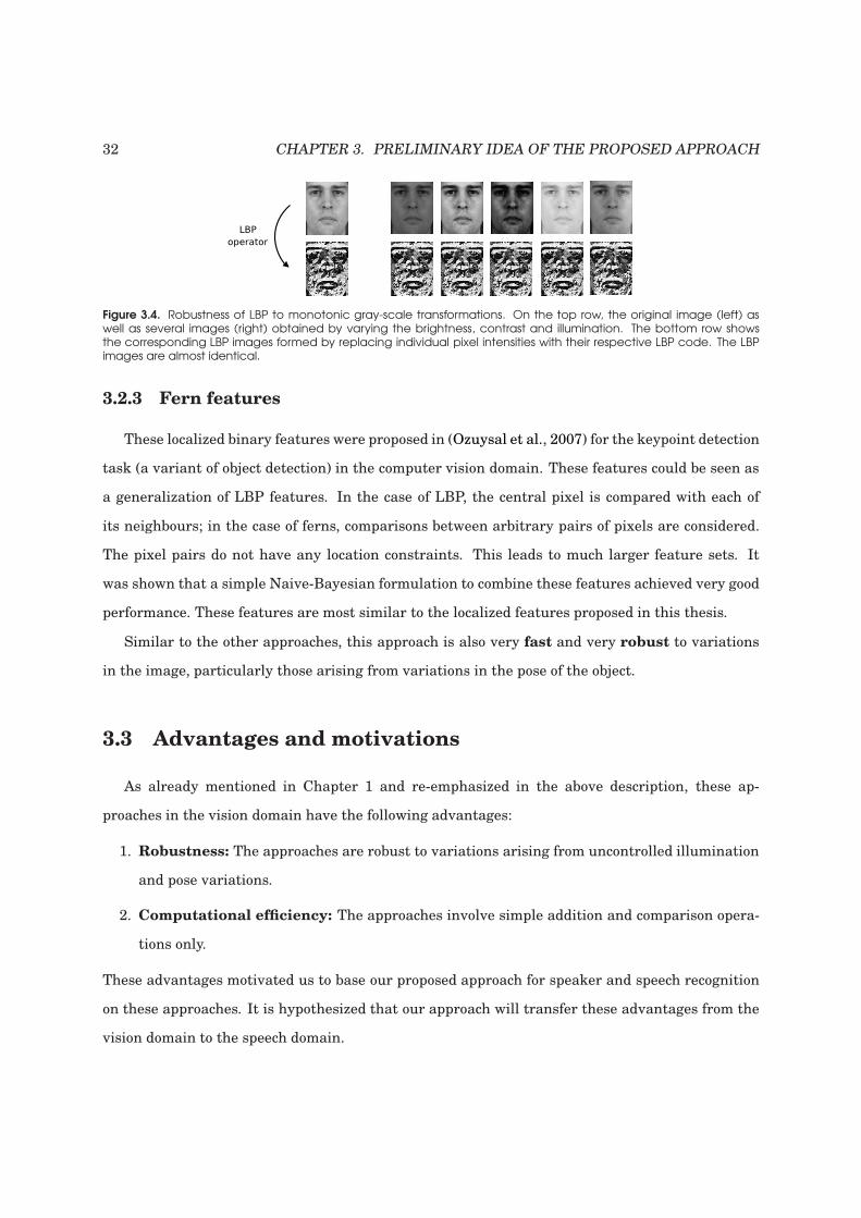
This robustness property is illustrated in Figure 3.4.
3. Similar to Haar features, such features can also be coupled with a simple modeling mod-
ule (Rodriguez, 2006). Hence, it is fast.
3. This is similar to the property of digital signals, whose value is unchanged as long as the noise affecting the signalremains below the quantization threshold.
32 CHAPTER 3. PRELIMINARY IDEA OF THE PROPOSED APPROACH
Figure 3.4. Robustness of LBP to monotonic gray-scale transformations. On the top row, the original image (left) aswell as several images (right) obtained by varying the brightness, contrast and illumination. The bottom row showsthe corresponding LBP images formed by replacing individual pixel intensities with their respective LBP code. The LBPimages are almost identical.
3.2.3 Fern features
These localized binary features were proposed in (Ozuysal et al., 2007) for the keypoint detection
task (a variant of object detection) in the computer vision domain. These features could be seen as
a generalization of LBP features. In the case of LBP, the central pixel is compared with each of
its neighbours; in the case of ferns, comparisons between arbitrary pairs of pixels are considered.
The pixel pairs do not have any location constraints. This leads to much larger feature sets. It
was shown that a simple Naive-Bayesian formulation to combine these features achieved very good
performance. These features are most similar to the localized features proposed in this thesis.
Similar to the other approaches, this approach is also very fast and very robust to variations
in the image, particularly those arising from variations in the pose of the object.
3.3 Advantages and motivations
As already mentioned in Chapter 1 and re-emphasized in the above description, these ap-
proaches in the vision domain have the following advantages:
1. Robustness: The approaches are robust to variations arising from uncontrolled illumination
and pose variations.
2. Computational efficiency: The approaches involve simple addition and comparison opera-
tions only.
These advantages motivated us to base our proposed approach for speaker and speech recognition
on these approaches. It is hypothesized that our approach will transfer these advantages from the
vision domain to the speech domain.

3.4. LOCALIZED APPROACHES IN SPEECH 33
3.4 Localized approaches in speech
Note that the approach presented in this thesis is not the first localized approach to be proposed
in the speech domain. In fact, there are already some systems in the speech domain which involve
localized features or localized processing of information (ref. Chapter 1). In this section, we review
some of these existing approaches in the speech domain.
3.4.1 Sub-band-based approach
Independent processing of speech in frequency sub-bands was inspired by the interpretation of
Fletchers work (Fletcher, 1953) by Allen (Allen, 1994). This idea was applied to ASR in (Bourlard
et al., 1996; Bourlard and Dupont, 1996). In this approach, class-conditional probabilities are es-
timated independently in frequency sub-bands. Due to this characteristic, this approach could be
termed “localized” in frequency bands.
This approach is shown to be specially applicable when the speech signal is partially degraded
by a frequency-selective noise. In this case, some part of the speech spectrum could still carry
useful information and the error in one frequency band is countered by the useful information in
other uncorrupted frequency bands.
This contrasts with standard cepstral features used in ASR which are holistic (ref. Chapter
2): even one or a few corrupted elements in the feature vector would lead to severe degradation of
recognition performance.
3.4.2 TempoRAl PatternS (TRAPS)
This approach is described in (Sharma and Hermansky, 1999). It uses longtime temporal pat-
terns (TRAPs) of critical band spectral energies in place of standard spectral patterns used for ASR.
Similar to the sub-band approach, it processes individual spectral energies independently; hence,
it could also be termed as “localized” in frequency bands.
This approach yields information that is complementary to standard spectral features. A combi-
nation of this approach with the standard approach results in improved robustness to several types
of additive and convolutive noise.
34 CHAPTER 3. PRELIMINARY IDEA OF THE PROPOSED APPROACH
3.4.3 Gabor features
This approach inspired by studies of the human auditory cortex is proposed in (Kleinschmidt
and Gelbart, 2002). In this approach, two-dimensional Gabor functions, with varying extents and
tuned to different rates and directions of spectro-temporal modulation, are applied as filters to a
spectro-temporal representation provided by mel spectra.
This approach shows significant improvements in ASR performance on both clean and noisy
data when combined with the standard approach. It is noteworthy that this approach involves
data-driven feature selection which is also one of the aspects of the proposed system.
3.4.4 Acoustic object detection
This approach described in (Amit et al., 2005) was one of the first ones to treat ASR as an
acoustic object detection problem, porting ideas from the computer vision domain. The authors
consider phonemes or words as acoustic objects similar to visual objects like a face or a car in
computer vision systems (Froba and Ernst, 2004). The authors proposed a new approach to the
problem of detecting such acoustic objects using features localized in the time-frequency plane. It
was shown that this approach has built-in robustness to amplitude variations and time warping.
3.4.5 Parts-based models and local features
This approach (Schutte, 2009) was inspired by (Amit et al., 2005) and was considerably influ-
enced by previous work in computer vision. The authors developed a complete parts-based frame-
work for ASR as an alternative to the standard holistic approach. They used graphical models
to represent speech with a deformable template of spectro-temporally localized “parts”. A class of
features extracted from these parts are very similar to the Haar features commonly used for face
detection in the computer vision domain (Viola and Jones, 2001). It is noteworthy that this work
also investigated data-driven selection of features. The selection was based on boosting, a standard
approach in computer vision suitable for use with Haar features (Friedman et al., 1998).
Evaluation of the framework on isolated letter recognition tasks showed its benefits over stan-
dard systems, particularly in noisy conditions and when only limited training data is available.
Note that the problem of continuous speech recognition was not addressed in this work.
3.5. SUMMARY 35
3.4.6 Boosted Haar features for music identification
Although addressing neither speaker nor speech recognition, we mention this approach (Ke
et al., 2005) for the sake of completeness since it deals with the related problem of music iden-
tification. The authors addressed the problem by considering the spectrogram of a music clip as
a two-dimensional image, converting the problem of music identification into an image retrieval
problem.
Similar to (Schutte, 2009), this approach extracts a set of Haar features from the spectrogram.
A feature selection strategy based on boosting is used to learn the most discriminative of these
features from the data. The approach was shown to be accurate, significantly outperforming the
state-of-the-art in this domain, and also fast.
From the above description, it is evident that these localized approaches in the speech do-
main also show robustness (to a noisy environment). This parallels the robustness of localized
approaches in the computer vision domain and further motivates us to pursue our localized ap-
proach for speaker and speech recognition. Note that our proposed approach is largely distinct
from these existing localized approaches in speech. 4
3.5 Summary
This chapter provided a preliminary idea of the proposed approach. We listed the fundamental
characteristics of this approach and described existing approaches in the computer vision domain
which inspired this work. It is observed that these approaches in the computer vision domain are
robust and computationally efficient. These aspects are the main motivations of this work.
It was also shown that a certain amount of work has been done in the speech domain involving
localized processing of information. These approaches also share the characteristic of robustness
(to noise).
The next chapter describes the proposed approach in detail.
4. It shares some similarities with the approach by Schutte et al. in the use of spectro-temporal representations of speech.However, the binary features and subsequent processing are substantially different from this work.

36 CHAPTER 3. PRELIMINARY IDEA OF THE PROPOSED APPROACH
Chapter 4
The proposed approach for
speaker and speech recognition
In this chapter, we describe the proposed approach for speaker and speech recognition. Simi-
lar to the standard approach, this has three modules: 1) Feature extraction, 2) Modeling, and 3)
Decision-making. This chapter provides a generic description of the approach: often a range of op-
tions and parameter values are provided instead of specifying a single one. These will be specified
to suit specific applications (speaker or speech recognition) in the subsequent chapters.
4.1 The proposed approach: Boosted Binary Features (BBF)
In this approach, the difference in magnitude at two distinct time-frequency points in the
spectro-temporal representation of speech is quantized to a binary (±1) value by comparing it with
a threshold. This binary value is considered as a feature. All possible pairs of time-frequency points
and all possible thresholds lead to a very large number of such binary features.
Modeling consists of a linear weighted summation of these binary features. Iterative minimiza-
tion of a loss function associated with this linear summation model leads to the selection of a small
subset of these features via the Discrete Adaboost algorithm (Friedman et al., 1998). These selected
features are termed as Boosted Binary Features (BBF). In the simplest case, decision-making con-
sists of a comparison of this linear summation to a threshold; the comparison outcome predicts the
37
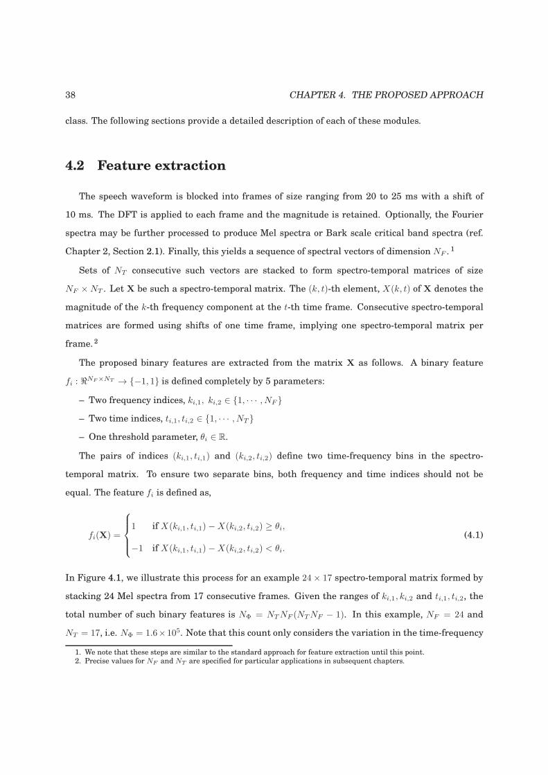
38 CHAPTER 4. THE PROPOSED APPROACH
class. The following sections provide a detailed description of each of these modules.
4.2 Feature extraction
The speech waveform is blocked into frames of size ranging from 20 to 25 ms with a shift of
10 ms. The DFT is applied to each frame and the magnitude is retained. Optionally, the Fourier
spectra may be further processed to produce Mel spectra or Bark scale critical band spectra (ref.
Chapter 2, Section 2.1). Finally, this yields a sequence of spectral vectors of dimension NF .1
Sets of NT consecutive such vectors are stacked to form spectro-temporal matrices of size
NF ×NT . Let X be such a spectro-temporal matrix. The (k, t)-th element, X(k, t) of X denotes the
magnitude of the k-th frequency component at the t-th time frame. Consecutive spectro-temporal
matrices are formed using shifts of one time frame, implying one spectro-temporal matrix per
frame. 2
The proposed binary features are extracted from the matrix X as follows. A binary feature
fi : ℜNF×NT → −1, 1 is defined completely by 5 parameters:
– Two frequency indices, ki,1, ki,2 ∈ 1, · · · , NF
– Two time indices, ti,1, ti,2 ∈ 1, · · · , NT
– One threshold parameter, θi ∈ R.
The pairs of indices (ki,1, ti,1) and (ki,2, ti,2) define two time-frequency bins in the spectro-
temporal matrix. To ensure two separate bins, both frequency and time indices should not be
equal. The feature fi is defined as,
fi(X) =
1 if X(ki,1, ti,1)−X(ki,2, ti,2) ≥ θi,
−1 if X(ki,1, ti,1)−X(ki,2, ti,2) < θi.
(4.1)
In Figure 4.1, we illustrate this process for an example 24× 17 spectro-temporal matrix formed by
stacking 24 Mel spectra from 17 consecutive frames. Given the ranges of ki,1, ki,2 and ti,1, ti,2, the
total number of such binary features is NΦ = NTNF (NTNF − 1). In this example, NF = 24 and
NT = 17, i.e. NΦ = 1.6×10⁵. Note that this count only considers the variation in the time-frequency
1. We note that these steps are similar to the standard approach for feature extraction until this point.2. Precise values for NF and NT are specified for particular applications in subsequent chapters.
4.3. MODELING AND DECISION-MAKING 39
Time index
Fre
quen
cy(M
elfilt
er)
index
Spectro-temporal matrix X
2 4 6 8 10 12 14 16
5
10
15
20
Σ
+1
-1-1
+1
θi
ti,1 = 11ti,2 = 3
X(ki,1, ti,1)
ki,2 = 6
ki,1 = 22
X(ki,2, ti,2)
Binaryfeature
Figure 4.1. Each binary feature fi is associated with a pair of time-frequency bins in the spectro-temporal matrix,defined by the parameters (ki,1, ti,1) and (ki,2, ti,2). The difference of the values at these two bins is compared witha threshold θi and the sign is retained. An example feature fi is shown in the figure. In this case, the spectra are Melspectra, with NF = 24 and NT = 17. Please see Section 4.2 for more details.
indices. Varying the thresholds leads to a further increase in this number. Let Φ = fiNΦ
i=1 represent
the complete set of such features. 3
In fact, out of the complete set Φ, only a small subset of features need to be finally extracted.
This will be further elaborated in subsequent sections.
4.3 Modeling and decision-making
The modeling module is very simple. It comprises of a linear weighted summation of the binary
features fi. The summation F is calculated as:
F (X) =∑
fi∈Φ∗
αifi(X) (4.2)
where αi is the weight associated with the binary feature fi. Note that only a subset of features Φ∗
out of the complete set Φ is used in the summation.
3. The complete set Φ could be considered as a projection from the original feature space to a high-dimensional featurespace.
40 CHAPTER 4. THE PROPOSED APPROACH
For now, we consider the two class case: for example, client and impostor class in speaker recog-
nition. In the decision-making module, F is used as a classifier function and its sign is used to
predict the class Ω∗ as follows,
Ω∗ =
Ω1 (predict class ‘1’) if F (X) ≥ 0,
Ω0 (predict class ‘0’) otherwise.
(4.3)
where classes ‘1’ and ‘0’ (or, Ω1 and Ω0) denote generic classes. For example, they could be client or
impostor class in the case of speaker recognition, or a particular phoneme or phonemes in the case
of speech recognition. This is the basic decision-making module.
Until now, we did not specify how to select the subset of features Φ∗ used to calculate the sum-
mation F . Also, we did not specify how the weights αi in Equation 4.2 are set. These two steps
are explained in the next section.
4.4 Feature Selection
The main objective of the system is to perform correct classification, i.e. minimize the misclassi-
fication loss given the summation F as defined earlier:
Lmisc,F =1
Ntr
Ntr∑
j=1
1F (Xj)y(Xj)<0 (4.4)
where the label y(Xj) = 1 if Xj belongs to class Ω1 and y(Xj) = −1 if X belongs to class Ω0.
The summation is over the set XjNtr
j=1 all Ntr training samples. The misclassification loss Lmisc,F
simply computes the total number of misclassification errors over all the training samples. It is not
tractable to minimize this loss directly. However, since 1F (X)y(X)<0 ≤ e−F (X)y(X), the exponential
loss is minimized instead:
Lexp,F =1
Ntr
Ntr∑
j=1
e−F (Xj)y(Xj) (4.5)
The exponential loss is an upper bound on the misclassification loss. The exponential loss is min-
imized using the Discrete Adaboost algorithm with weighted resampling (Friedman et al., 1998;
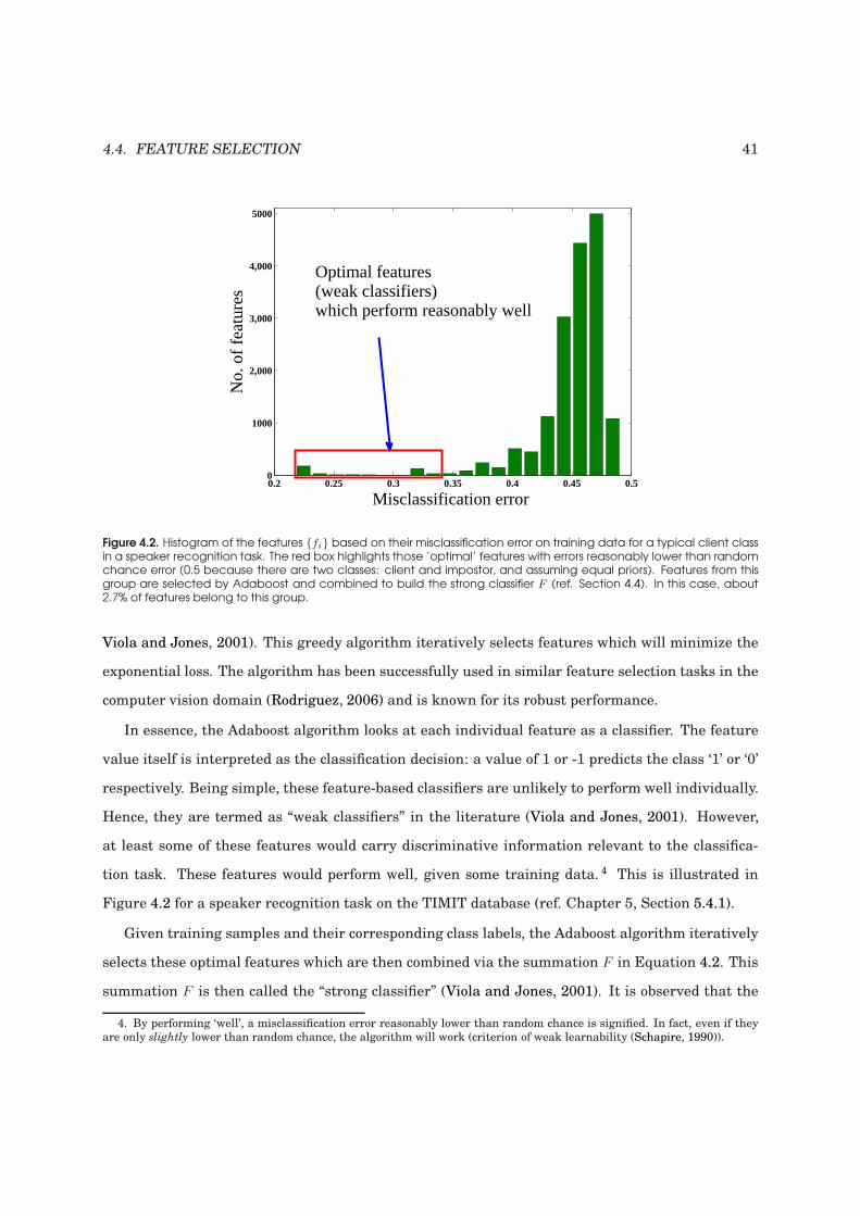
4.4. FEATURE SELECTION 41
0.2 0.25 0.3 0.35 0.4 0.45 0.50
1000
2,000
3,000
4,000
5000
Misclassification error
No.
of f
eatu
res
Optimal features (weak classifiers)which perform reasonably well
Figure 4.2. Histogram of the features fi based on their misclassification error on training data for a typical client classin a speaker recognition task. The red box highlights those ‘optimal’ features with errors reasonably lower than randomchance error (0.5 because there are two classes: client and impostor, and assuming equal priors). Features from thisgroup are selected by Adaboost and combined to build the strong classifier F (ref. Section 4.4). In this case, about2.7% of features belong to this group.
Viola and Jones, 2001). This greedy algorithm iteratively selects features which will minimize the
exponential loss. The algorithm has been successfully used in similar feature selection tasks in the
computer vision domain (Rodriguez, 2006) and is known for its robust performance.
In essence, the Adaboost algorithm looks at each individual feature as a classifier. The feature
value itself is interpreted as the classification decision: a value of 1 or -1 predicts the class ‘1’ or ‘0’
respectively. Being simple, these feature-based classifiers are unlikely to perform well individually.
Hence, they are termed as “weak classifiers” in the literature (Viola and Jones, 2001). However,
at least some of these features would carry discriminative information relevant to the classifica-
tion task. These features would perform well, given some training data. 4 This is illustrated in
Figure 4.2 for a speaker recognition task on the TIMIT database (ref. Chapter 5, Section 5.4.1).
Given training samples and their corresponding class labels, the Adaboost algorithm iteratively
selects these optimal features which are then combined via the summation F in Equation 4.2. This
summation F is then called the “strong classifier” (Viola and Jones, 2001). It is observed that the
4. By performing ‘well’, a misclassification error reasonably lower than random chance is signified. In fact, even if theyare only slightly lower than random chance, the algorithm will work (criterion of weak learnability (Schapire, 1990)).
42 CHAPTER 4. THE PROPOSED APPROACH
strong classifier performs quite well, and much better than the individual weak classifiers (Fried-
man et al., 1998). In fact, the algorithm progressively reducesmisclassification error on the training
data with each new feature selected (Friedman et al., 1998). Furthermore, it is often observed that
the test error continues to reduce even when the training error saturates. An overview of the main
steps of the Adaboost algorithm is provided next.
The algorithm works in a loop. In each iteration of the loop, it selects one feature out of the
complete set of features Φ based on how well it performs on a subset of training samples which
were misclassified in previous iterations. Each iteration has three steps:
1. Select a fixed number N∗tr of training samples based on their weights. 5 Samples with higher
weights are more likely to be selected.
2. Select the feature (weak classifier) which performs best on this subset of training samples.
3. Classify all the training samples using this selected feature and re-weight all of them, so that
misclassified samples’ weights are proportionately increased, and correctly classified ones’
weight are decreased.
In addition to selecting the feature, each iteration also assigns a weight to the selected feature,
based on its efficiency. Note that this is different from the training sample weights. The iterations
stop when the required number of features NΦ∗ have been selected. Suitable values for the number
NΦ∗ is provided in subsequent chapters.
Two important aspects of the algorithm are worthy of note: 1) Feature selection and modeling
are linked. The re-weighting of training samples based on prior classification performance serves
as the feedback link between feature selection and feature modelling. This means that even fea-
ture extraction and modeling are linked, because in practice, only the selected features are to be
extracted. 2) Feature selection is data-driven and class (or problem) specific. The algorithm is now
described below in details.
5. Initially, the sample weights are all uniform. Note that in this case, each training sample is actually a spectro-temporalmatrix.

4.4. FEATURE SELECTION 43
Discrete Adaboost algorithm for two-class problem (classes Ω1 and Ω0)
Inputs: Ntr training samples, i.e. spectro-temporal matrices XjNtr
j=1 extracted from the training
speech data; their corresponding class labels, yj ∈ −1, 1, (−1 : Xj ∈ Ω0, 1 : Xj ∈ Ω1); N∗tr,
the number of training samples to be randomly sampled at each iteration (N∗tr < Ntr).
6 NΦ∗ , the
number of features to be selected;
Steps:
1. Initialize the sample weights w1,j ←1
Ntr.
2. Repeat for n = 1, 2, · · ·NΦ∗ :
(a) Normalize the sample weights, wn,j ←wn,j
∑Ntrj′=1
wn,j′
(b) Randomly sample a subset of N∗tr training samples, according to the distribution wn,j
(c) For each feature fi in Φ, set the threshold parameter θi to minimize misclassification
error,
ei =1
N∗tr
∑N∗tr
j=1 1fi(Xj) 6=yj over the sampled subset. 7
(d) Select the next best feature, f∗n = f∗
i
where i∗ = argmini ei, i.e. select that feature which the lowest misclassification error on
the current subset of training samples.
(e) Set βn ←ei∗
1−ei∗
(f) Set the weight of the selected feature,
αn = − log(βn).
(g) Update the sample weights,
wn+1,j ← wn,jβ1f∗
n(Xj)=yj
n
3. Normalize feature weights to sum to one,
αn ←αn
∑N∗L
n′=1αn′
, for 1 ≤ n ≤ N∗L.
Output: The set of selected best features Φ∗ ≡ f∗n, α
∗n
NΦ∗
n=1 .
6. A value of N∗
tr equal to 5% of Ntr was found to work well for all experiments reported here in subsequent chapters.7. The difference Xj(ki,1, ti,1)−Xj(ki,2, ti,2) for each training sample Xj is taken as a candidate threshold value. Any
value in between two consecutive such thresholds would not change the classification result and hence can be ignored. Theoptimal threshold θi is chosen via a search over these candidate values.
44 CHAPTER 4. THE PROPOSED APPROACH
The selected features (Φ∗) are termed as Boosted Binary Features (BBF) since they are se-
lected via Adaboost.
The selected features and their weights are then used in Equation 4.2 to calculate the strong
classifier summation F . In 4.3, this summation was compared with zero. In actual practice, it is
compared with a separate threshold Θ to predict the class:
Ω∗ =
Ω1 (predict class ‘1’) if F (X) ≥ Θ,
Ω0 (predict class ‘0’) otherwise.
(4.6)
The threshold Θ is set using a suitable error criterion. For instance, the Equal Error Rate for
speaker recognition (Reynolds, 1995).
Equation 4.6 describes the decision-making process for an individual spectro-temporal matrix
X. In practical applications, a decision is required corresponding to a sequence of such matrices
and not from a single matrix. For example, in the case of speaker verification, a decision is re-
quired from all the spectro-temporal matrices extracted from an utterance made by the speaker.
The method of combining the decisions from multiple spectro-temporal matrices depends on the
particular application involved. It is described in subsequent chapters.
This completes the description of the modeling and decision-making module of the proposed
framework.
4.5 Summary
In this chapter, we described the proposed approach for speaker and speech recognition. The
approach involves a boosted ensemble of binary features extracted by thresholding the differences
in magnitude at two time-frequency bins on the spectro-temporal representation of speech. These
features are called Boosted Binary Features and henceforth, this approach shall be called as the
BBF approach.
Now, we can summarize again the four characteristics of the proposed approach mentioned in
Chapter 3:
1. The proposed features are localized. This is because each feature fi looks at two specific time-

4.5. SUMMARY 45
frequency points in the spectro-temporal matrix. 8
2. The features are binary (±1).
3. The approach is data-driven. A subset of features are selected from the complete set using the
Discrete Adaboost algorithm. The selected features are the ones which are most discrimina-
tive with respect to the specific class.
4. There is a strong link between the feature extraction and modeling modules. The link appears
through the feature selection process which iteratively selects features that perform well on
previously misclassified training samples based on the current model. Only the selected fea-
tures are then extracted during feature extraction.
In the subsequent chapters, we describe two applications of this approach: 1) speaker recognition,
and 2) speech recognition.
8. Although the features are localized, no frequency band is ignored, since all the features together look at all the differentregions in the spectrum.

46 CHAPTER 4. THE PROPOSED APPROACH
Chapter 5
Application of proposed approach
to Speaker Recognition
In this chapter, we describe the application of the proposed Boosted Binary Features (BBF) ap-
proach to the task of speaker recognition. Speaker recognitionmay mean either speaker verification
(SV) or speaker identification (SI). As mentioned in Chapter 1, in this thesis, speaker recognition
always signifies speaker verification and the two words “speaker recognition” and “speaker verifi-
cation” are used interchangeably.
We begin by discussing some of the current objectives related to the speaker recognition task and
how they motivate this work. Next, we show how the generic system described in Chapter 4 is tuned
specifically for the speaker recognition task. A wide range of speaker recognition experiments are
then reported. These experiments evaluate the speaker recognition performance of the proposed
system and compare it with standard ones. Finally, we discuss some of the interesting aspects of
the proposed approach relevant to the speaker recognition task.
5.1 Objectives and motivations
Today, speaker recognition systems are gradually becoming more and more ubiquitous. They
are finding their way into mobile phones and other portable devices (Marcel et al., 2010b,a). This
has led to the following objectives:
47
48 CHAPTER 5. APPLICATION TO SPEAKER RECOGNITION
1. To ensure robustness of the system against a noisy acoustic environment (additive noise) as
well as channel and session variabilities. This is because a portable device is liable to be used
everywhere, even in very noisy environments like railway stations and airports.
2. To keep the computations light enough to be implementable on such devices. This is because
such devices still have lower computing resources than standard desktop computers.
To fulfill the first objective mentioned above, i.e. robustness, state-of-the-art speaker recognition
systems improve upon the baseline GMM framework described in Section 2.2.1 as follows: a) in the
feature extraction module by using short-time Gaussianization (Chen and Gopinath, 2000) or fea-
ture warping (Pelcanos and Sridharan, 2001), b) in the modeling module by using meta-modelling
approaches such as Support Vector Machines with GMM Supervector (GSV) kernel (Campbell
et al., 2006) or Generalized Linear Discriminant Sequence (GLDS) kernel (Campbell, 2002), La-
tent Factor Analysis (Matrouf et al., 2007), Joint Factor Analysis (Kenny et al., 2007) and I-vector
system (Dehak et al., 2009), and c) in the decision-making module by using score normalization
techniques (Auckenthaler et al., 2000) such as Z-norm and T-norm.
However, improved performance of such systems comes at the cost of increased computational
complexity. This may pose a problem with respect to the second objective mentioned earlier, i.e.
computational efficiency. Hence, the question is: how to fulfill both the objectives at the same time?
As mentioned in Chapter 3, Section 3.3, it is hypothesized that the proposed approach involving
Boosted Binary Features has the potential to satisfy both these objectives of robustness and com-
putational efficiency at the same time. This hypothesis motivates this work. It is tested through
experimental studies reported in later sections of this chapter.
5.2 Proposed BBF approach applied to speaker recognition
The proposed BBF approach described in Chapter 4 is directly applied to the speaker recognition
task (Roy et al., 2011a,c). The approach involves three modules: 1) feature extraction, 2) modeling
and 3) decision-making. Since the system is more or less the same as described in Chapter 4, here
we just describe each of these modules briefly, emphasizing how they are fine-tuned for the speaker
recognition task. 1
1. For easy understanding, the reader is encouraged to first read Chapter 4 which gives a detailed description of theapproach.
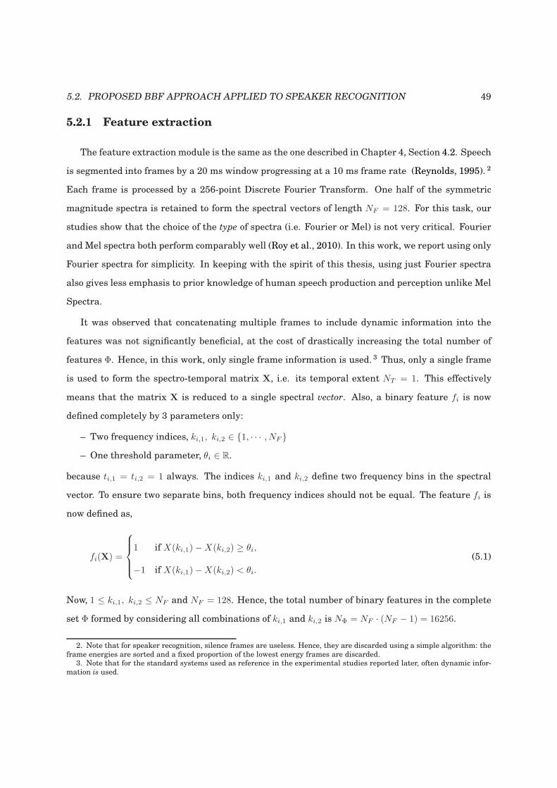
5.2. PROPOSED BBF APPROACH APPLIED TO SPEAKER RECOGNITION 49
5.2.1 Feature extraction
The feature extraction module is the same as the one described in Chapter 4, Section 4.2. Speech
is segmented into frames by a 20 ms window progressing at a 10 ms frame rate (Reynolds, 1995). 2
Each frame is processed by a 256-point Discrete Fourier Transform. One half of the symmetric
magnitude spectra is retained to form the spectral vectors of length NF = 128. For this task, our
studies show that the choice of the type of spectra (i.e. Fourier or Mel) is not very critical. Fourier
and Mel spectra both perform comparably well (Roy et al., 2010). In this work, we report using only
Fourier spectra for simplicity. In keeping with the spirit of this thesis, using just Fourier spectra
also gives less emphasis to prior knowledge of human speech production and perception unlike Mel
Spectra.
It was observed that concatenating multiple frames to include dynamic information into the
features was not significantly beneficial, at the cost of drastically increasing the total number of
features Φ. Hence, in this work, only single frame information is used. 3 Thus, only a single frame
is used to form the spectro-temporal matrix X, i.e. its temporal extent NT = 1. This effectively
means that the matrix X is reduced to a single spectral vector. Also, a binary feature fi is now
defined completely by 3 parameters only:
– Two frequency indices, ki,1, ki,2 ∈ 1, · · · , NF
– One threshold parameter, θi ∈ R.
because ti,1 = ti,2 = 1 always. The indices ki,1 and ki,2 define two frequency bins in the spectral
vector. To ensure two separate bins, both frequency indices should not be equal. The feature fi is
now defined as,
fi(X) =
1 if X(ki,1)−X(ki,2) ≥ θi,
−1 if X(ki,1)−X(ki,2) < θi.
(5.1)
Now, 1 ≤ ki,1, ki,2 ≤ NF and NF = 128. Hence, the total number of binary features in the complete
set Φ formed by considering all combinations of ki,1 and ki,2 is NΦ = NF · (NF − 1) = 16256.
2. Note that for speaker recognition, silence frames are useless. Hence, they are discarded using a simple algorithm: theframe energies are sorted and a fixed proportion of the lowest energy frames are discarded.
3. Note that for the standard systems used as reference in the experimental studies reported later, often dynamic infor-mation is used.
50 CHAPTER 5. APPLICATION TO SPEAKER RECOGNITION
5.2.2 Modeling and Decision-making
As described in Chapter 4, Section 4.3, the model involves a simple linear summation F of the
binary features:
F (X) =∑
fi∈Φ∗
αifi(X) (5.2)
The optimal feature set Φ∗ are selected and the weights αi are set as before by the Discrete
Adaboost algorithm (ref. Section 4.4) for each client speaker class. A few particular aspects about
this algorithm relevant to the speaker recognition task are worthy of note:
1. In this case, the positive training samples corresponding to class Ω1 (label y = 1) are extracted
from speech data coming from the specific client. The negative samples corresponding to class
Ω0 (label y = −1) come from a general pool of speakers, distinct from the client. The same set
of ‘impostor’ speakers termed the background set or world set are used for all clients. This
setup is similar to the case of the Universal BackgroundModel (UBM) framework for standard
speaker recognition systems (ref. Section 2.2.1).
2. Due to the re-weighting procedure in the algorithm, misclassified samples get more weight in
successive iterations. This implies that, in effect, more confusable speakers in the background
set are expected to get more importance, analogous to the idea of cohorts in the standard
approach (Reynolds, 1995)(ref. Section 2.2.1). However, in the case of the proposed approach,
the distinction between what is more easily- and less easily- classifiable is at the frame level,
not at the speaker level.
To provide an insight about the selected features, Figure 5.1 shows the client and impostor
distributions of the spectral differences corresponding to the first two binary features selected by
Adaboost for two client speakers from the standard TIMIT database (Fisher et al., 1986), one
female (‘F’) and one male (‘M’). More precisely, by difference hi we mean:
hi = X(ki,1)−X(ki,2) (5.3)
i.e. the difference in magnitude at the two frequency points X(ki,1) and X(ki,2 corresponding to
the feature fi. In this case, h1 and h2 are shown. We note that there exists regions of non-overlap
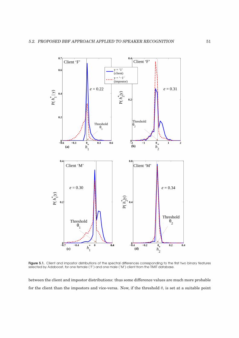
5.2. PROPOSED BBF APPROACH APPLIED TO SPEAKER RECOGNITION 51
−0.6 −0.3 0 0.3 0.60
0.2
0.4
0.6
0.7
h*1
P( h
* 1 | y)
−2 −1 0 1 20
0.2
0.4
h*2
P( h
* 2|y)
y = ‘1’(client)
y = ‘−1’(impostor)
(a) (b)
Client ‘F’ Client ‘F’
e = 0.22
Thresholdθ
2Threshold
θ1
e = 0.31
−0.7 −0.4 0 0.40.40
0.2
0.4
h*1
P( h
* 1|y)
−0.4 −0.2 0 0.2 0.40
0.4
0.8
h*2
P( h
* 2|y)
(c) (d)
Thresholdθ
1
Thresholdθ
2
e = 0.30 e = 0.34
Client ‘M’ Client ‘M’
Figure 5.1. Client and impostor distributions of the spectral differences corresponding to the first two binary featuresselected by Adaboost, for one female (‘F’) and one male (‘M’) client from the TIMIT database.
between the client and impostor distributions: thus some difference values are much more probable
for the client than the impostors and vice-versa. Now, if the threshold θi is set at a suitable point
52 CHAPTER 5. APPLICATION TO SPEAKER RECOGNITION
(as indicated in the figure), the resulting binary feature would be able to perform with moderately
low errors as indicated in the figure. This could be interpreted as client-specific discriminative
information contained in these features.
After feature selection by Adaboost, the selected features are combined through the summation
F as mentioned before. The summation is now termed the “strong classifier” (ref. Section 4.4) and
the feature selection process is referred to as classifier training. In the case of speaker recognition
task, a decision is only required at the utterance level and not at the frame level. Hence, for an
utterance U , the summation F (X) at every frame X in the utterance are added and normalized by
the number of frames NU in the utterance to obtain the mean summation score S:
S(U) =1
NU
∑
X∈U
F (X) (5.4)
During decision-making, instead of using the frame-level summation F (X), this mean score S is
compared with a preset threshold Θ. If S is higher than Θ, it is decided that the utterance was
made by the client (ie. the claim is accepted), or an impostor otherwise, i.e.:
Ω∗ =
Ω1 (predict ‘client’) if S ≥ Θ,
Ω0 (predict ‘impostor’) otherwise.
(5.5)
The threshold Θ is set to correspond to the Equal Error Rate (EER) (Reynolds, 1995; Bimbot et al.,
2004).
In Figure 5.2, we show the variation of the training error etr(Nf ) corresponding to this strong
classifier F as a function of the number of selected features Nf used in the summation. Here, the
training error is the total number of training examples misclassified (with equal priors for client
and impostor), based on the utterance level score (ref. Equation 5.5), averaged over all 168 clients
in the TIMIT database. The mean training error (calculated using a single global threshold Θ for
all clients) and the variation in error over individual clients have been plotted. We note that the
training error decreases quickly with increase in Nf . We will note in the experiment section that
this trend is also reflected in the test error. This completes the description of the proposed approach
as it is applied for speaker recognition in this thesis.
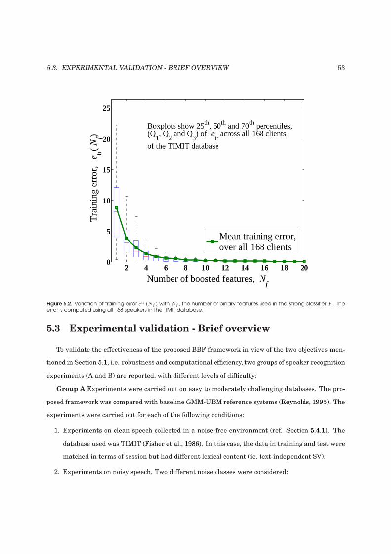
5.3. EXPERIMENTAL VALIDATION - BRIEF OVERVIEW 53
2 4 6 8 10 12 14 16 18 200
5
10
15
20
25
Number of boosted features, Nf
Tra
inin
g er
ror,
etr(
Nf)
Mean training error,over all 168 clients
Boxplots show 25th, 50th and 70th percentiles,(Q
1, Q
2 and Q
3) of e
tr across all 168 clients
of the TIMIT database
Figure 5.2. Variation of training error etr(Nf ) with Nf , the number of binary features used in the strong classifier F . Theerror is computed using all 168 speakers in the TIMIT database.
5.3 Experimental validation - Brief overview
To validate the effectiveness of the proposed BBF framework in view of the two objectives men-
tioned in Section 5.1, i.e. robustness and computational efficiency, two groups of speaker recognition
experiments (A and B) are reported, with different levels of difficulty:
Group A Experiments were carried out on easy to moderately challenging databases. The pro-
posed framework was compared with baseline GMM-UBM reference systems (Reynolds, 1995). The
experiments were carried out for each of the following conditions:
1. Experiments on clean speech collected in a noise-free environment (ref. Section 5.4.1). The
database used was TIMIT (Fisher et al., 1986). In this case, the data in training and test were
matched in terms of session but had different lexical content (ie. text-independent SV).
2. Experiments on noisy speech. Two different noise classes were considered:
54 CHAPTER 5. APPLICATION TO SPEAKER RECOGNITION
(a) Additive noise (ref. Section 5.4.2). Database used was TIMIT. Three types of noise (white,
pink and babble) at SNRs ranging from 5dB to 20dB were added only to the test segments.
(b) Convolutive noise (ref. Section 5.4.3). Database used was HTIMIT (Reynolds, 1997).
Eight different microphone types were considered while testing.
These experiments involved a mismatch between training (using only clean speech) and test
(using noisy speech). However, this mismatch was artificially induced in the data. 4
Group B Experiments were carried out on the more challenging and recent MOBIO
database (Marcel et al., 2010a) (Section 5.5). The proposed framework was compared with multiple
state-of-the-art reference systems unlike only baseline systems as in Group A. These experiments
involved speech data collected using mobile phones and there was mismatch at multiple levels in
the data. This mismatch was naturally created as a direct consequence of the recording scenario, in
contrast to Group A. Lexical content of training and test speech was different, hence this was also
a text-independent SV problem.
Each of these experiments are described further in the following sections.
5.4 Group A Experiments
This group of experiments involved easy to moderately difficult conditions.
5.4.1 Experiments on clean speech: matched condition
The main aim here was to examine how well the proposed system can perform text-independent
speaker recognition with large populations under near-ideal conditions. The proposed system was
compared with a baseline reference system that used standard MFCC features modeled by GMMs
(ref. Chapter 2). 5
4. This was done by either adding the noise signal to the clean speech, or by playing the original speech and recording itby different types of microphones.
5. This could be seen as an extension of previous studies on the XM2VTS database (Roy et al., 2010) to the text-independent case. These previous studies had shown that the proposed system performed well but were limited by thefact that the lexical content in training and test were the same, ie. it was not known how the system could perform in thecase of text-independent speaker verification.

5.4. GROUP A EXPERIMENTS 55
Database description
The TIMIT database was chosen for this part of the work (Fisher et al., 1986). It is a stan-
dard database with no intersession variability, acoustic noise or microphone variability (Reynolds,
1995). Each utterance is a read sentence of approximately 3 seconds duration. The training and
test sentences have different lexical content, hence this is an example of text-independent speaker
recognition. The sampling frequency is 16kHz.
Systems evaluated, protocol and experimental details
To compare the proposed BBF system, the standard MFCC-GMM system detailed in (Reynolds,
1995) was chosen as reference. The speaker verification protocol as used by Reynolds et al. in
(Reynolds, 1995) was followed. The 168 speakers (112 males, 56 females) from the “test” portion of
the TIMIT database were used as clients. For each speaker, the 2 sa sentences, 3 si sentences and
first 3 sx sentences were used for training and the remaining 2 sx sentences for testing.
For all systems, speech was segmented into frames by a 20 ms window progressing at a 10
ms frame rate (Reynolds, 1995). For the BBF system, each frame was processed by a 256-point
Discrete Fourier Transform as mentioned in Section 5.2.1. One half of the symmetric magnitude
spectra was retained to form the spectral vectors X of length NF = 128.
For training a client classifier in the BBF system, i.e. to select the binary features using the
Adaboost algorithm (ref. Section 5.2.2), the positive (client, ‘1’) training samples were extracted
from the client training data, while the negative (impostor, ‘0’) samples were extracted from a set
of 250 utterances randomly selected from the “train” portion of the TIMIT database. The speakers
who made these utterances were all distinct from those in the “test” portion of the database and the
same negative samples were used for all the clients. We term this set of speakers as the “world” set
(ref. Section 5.2.2).
As mentioned earlier, the BBF system was compared with a standard MFCC-GMM system
(Reynolds, 1995). For clarity, we describe here only the main aspects of this system. Firstly, 12th or-
der Mel-frequency cepstral coefficients (MFCC) were extracted from the speech frames (Reynolds,
1992; Reynolds and Rose, 1995). These were then modelled by 32-mixture GMM (Reynolds, 1995).
To model impostors, each client had its own specific “world” or “background” set 6 of speakers, se-
6. This is alternatively termed the “cohort” set (Bimbot et al., 2004).
56 CHAPTER 5. APPLICATION TO SPEAKER RECOGNITION
lected from the set of clients itself (Reynolds, 1995). Depending on the selection criterion of the
background speakers, two reference system configurations were considered, namely
1. Reference system TI: 10 “maximally spread close” (msc) background speakers were selected.
2. Reference system TII: 5 msc + 5 “maximally spread far” (msf) background speakers were
selected.
During testing, the mean log-likelihood of the 10 background set models is subtracted from the log-
likelihood of the claimed client model (Reynolds, 1995) to estimate the log-likelihood ratio score of
a test utterance.
For evaluating the BBF system, experiments were performed using each of the 168 speakers
acting as the claimant, with each of the remaining 167 speakers acting as impostors, and rotating
through all speakers. Since the negative samples in training came from a distinct “world” set, all
the remaining 167 speakers were treated as impostors. For testing the reference systems TI and
TII, the same experiments were performed as for the BBF system, excluding the 10 background
speakers for each client from the impostors because these systems did not use a single distinct
“world” set as the BBF system.
Experiments were conducted separately for three conditions (Reynolds, 1995):
1. Mixed sex (F+M), using all 168 speakers.
2. Male only (M) (112 speakers).
3. Female only (F) (56 speakers).
The performance of a system was calculated in terms of the global Equal Error Rate (EER)
computed using a client-independent threshold (Reynolds, 1995) on the test data. For this, the
threshold Θ (ref. Section 5.2.2) at which the false-acceptance (FA) rate equals the false-rejection
(FR) rate is calculated, considering all client and impostor test scores together, and the FA using
this threshold is reported as the EER.
Thus, the global EER measures the overall (client-independent) performance of the system and
is likely to be much more statistically significant than results based on client-dependent thresholds
(Reynolds, 1995). 7 We did not re-implement the reference systems TI and TII. We directly report
here the results of the systems from (Reynolds, 1995).
7. Henceforth, we shall use EER to mean global EER.
5.4. GROUP A EXPERIMENTS 57
It is to be noted that the reference systems TI and TII use partially different data for training
and test compared to the BBF system with respect to impostors: 1) During training, the reference
systems use client-dependent “world” sets to model impostors, while the BBF system uses a single
“world” set of speakers to model impostors for all the clients. 2) During testing, the reference sys-
tems leave out the 10 background speakers used to model impostors for a particular client speaker
when evaluating its model, while the BBF system uses all the speakers in the client set. Hence,
one might suggest that the experimental setup is not precisely matched between the two systems
with respect to impostors. In fact, we did implement a third reference system using a Universal
Background Model - Maximum a posteriori Adaptation (UBM-MAP) paradigm (Section 2.2.1). This
system used the same single “world” set to model impostors as the BBF system and hence the same
data partitioning as the BBF system. But this system did not perform as well as TI and TII. Hence,
we chose to report here only the best performing systems, TI and TII.
Results
The EER of the systems have been shown in Figure 5.3 (a)-(c). For the BBF system, the EER has
been plotted against the number of binary features Nf selected by Adaboost and used to form the
final strong classifier F (ref. Section 5.2.2). In all the three experimental conditions, the proposed
BBF system has performed equally well as or very close to the reference systems.
The EER of the BBF system drops quickly from above 5% when less that ten binary features
are selected to below 1% after about 250 binary features are selected. For all 3 conditions, the
EER consistently shows a downward trend with increasingNf , interspersed with small oscillations,
finally reaching a saturation level. 8
This saturation level is close to the EER achieved by reference system TII for all 3 cases. For
the F+M case, it is slightly lower than the TI EER while for the M only and F only cases, it is
slightly higher than the TI EER. This saturation level is reached after about 400 to 450 binary
features have been selected. At this value of Nf , the computational complexity of the BBF system
is significantly lower than the reference systems.
8. Although results for only the first 500 binary features are shown in Figure 5.3, we conducted experiments using up to1000 binary features and the test EER still remained stable.
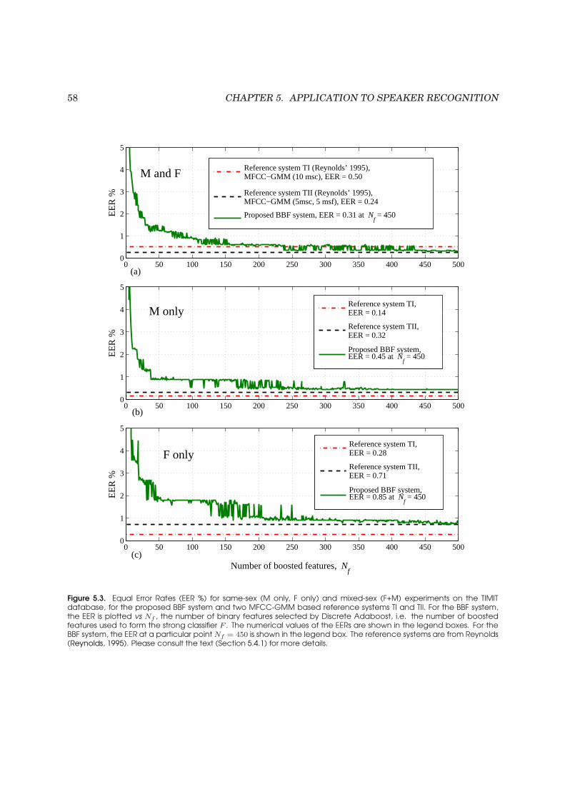
58 CHAPTER 5. APPLICATION TO SPEAKER RECOGNITION
0 50 100 150 200 250 300 350 400 450 5000
1
2
3
4
5
EE
R %
0 50 100 150 200 250 300 350 400 450 5000
1
2
3
4
5
EE
R %
0 50 100 150 200 250 300 350 400 450 5000
1
2
3
4
5
Number of boosted features, Nf
EE
R %
Reference system TI (Reynolds’ 1995),MFCC−GMM (10 msc), EER = 0.50
Reference system TII (Reynolds’ 1995),MFCC−GMM (5msc, 5 msf), EER = 0.24
Proposed BBF system, EER = 0.31 at Nf = 450
Reference system TI,EER = 0.14
Reference system TII,EER = 0.32
Proposed BBF system,EER = 0.45 at N
f = 450
Reference system TI,EER = 0.28
Reference system TII,EER = 0.71
Proposed BBF system,EER = 0.85 at N
f = 450
(a)
(b)
(c)
M and F
M only
F only
Figure 5.3. Equal Error Rates (EER %) for same-sex (M only, F only) and mixed-sex (F+M) experiments on the TIMITdatabase, for the proposed BBF system and two MFCC-GMM based reference systems TI and TII. For the BBF system,the EER is plotted vs Nf , the number of binary features selected by Discrete Adaboost, i.e. the number of boostedfeatures used to form the strong classifier F . The numerical values of the EERs are shown in the legend boxes. For theBBF system, the EER at a particular point Nf = 450 is shown in the legend box. The reference systems are from Reynolds(Reynolds, 1995). Please consult the text (Section 5.4.1) for more details.
5.4. GROUP A EXPERIMENTS 59
5.4.2 Experiments on speech corrupted by additive noise: mismatched
condition
The aim here was to examine the effect of mismatched additive noise on the performance of the
proposed system, compared to a standard MFCC-GMM system.
Database description
The TIMIT database (Fisher et al., 1986) was used in this part of the work also. As before,
the training and test sentences had different lexical content, hence this is also an example of text-
independent speaker recognition. The original clean TIMIT data was used only for training. For
testing, TIMIT data corrupted by additive noise was used. For this, three types of noise from the
Noisex-92 database (Varga et al., 1992), namely, white, pink and babble, were added to each test
utterance at four SNR levels (20dB, 15dB, 10dB and 5dB). 9 Hence, it was a mismatched testing
scenario.
Systems evaluated, protocol and experimental details
Apart from the proposed system, a standard MFCC-GMM system (Bimbot et al., 2004) was used
as the reference. 10 The BBF system was precisely the same as that used in Section 5.4.1.
Instead of the client-dependent background set described in Section 5.4.1 and (Reynolds, 1995),
we used a common impostor set to create a single GMM model called the Universal Background
Model (UBM) to model impostors (Section 2.2.1). The advantage for large speaker databases is that
individual background sets need not be selected for each client. 11
For fair comparison, this common impostor set is the same as the “world” set which provided
the negative samples for the BBF system (ref. Section 5.4.1) extracted from the “train” part of
TIMIT. For each client, a client model is created by adapting the means in the UBM using the client
training data (Bimbot et al., 2004).
For the reference MFCC-GMM system, we experimented using different number of cepstral co-
efficients (12 and 16) (Bimbot et al., 2004; Reynolds and Rose, 1995) for the features and different
9. The noise segments were randomly chosen and were equal in length to the test segments.10. In this case, we implemented the reference system ourselves.11. The single background model has become the predominant approach used in speaker verification systems (Bimbot
et al., 2004).
60 CHAPTER 5. APPLICATION TO SPEAKER RECOGNITION
number of Gaussians (from 32 to 1024) for the GMM. Among the different configurations of refer-
ence systems tried, we report here the two overall best performing ones:
1. Reference system NTI: 16 MFCC + 16∆MFCC + ∆Energy, Cepstral Mean Subtraction (CMS)
(Bimbot et al., 2004) and 1024-mixture GMM.
2. Reference system NTII: 12 MFCC (Reynolds, 1992; Reynolds and Rose, 1995), no delta, no
CMS, and 1024-mixture GMM.
The features used by the system NTII are the same as the reference systems in Section 5.4.1
(Reynolds and Rose, 1995) while the features used by system NTI involve slightly more calcula-
tions (Bimbot et al., 2004).
The same speaker verification protocol as used in Section 5.4.1 was followed (Reynolds, 1995).
The experimental details were exactly the same as in Section 5.4.1 except for one difference: all the
data for training came from original TIMIT database, while for test, different types of noise from
the Noisex-92 database was added to it. Apart from this, in this experiment, all the remaining 167
speakers were used as impostors even for the reference systems since they used the distinct “world”
impostor set for training, like the BBF system.
Separate experiments for the 3 different noise types at 4 different SNR levels were conducted,
leading to 12 different conditions. In the face of this, experiments were conducted for mixed sex
(F+M) condition only, using all 168 speakers (Reynolds, 1995). The performance of the systems was
calculated in terms of the global equal-error rate (EER) as before.
Results
The EER of the systems have been shown in Figure 5.4 (a)-(l). For the BBF system, the EER
has been plotted vs. the number of binary features selected, Nf . For all the 3 noise types and 4
SNR levels, the proposed BBF system has performed equally well as or better than the reference
systems. As in Section 5.4.1, the EER of the BBF system has shown a general downward trend
with increasing Nf although the errors are much higher here due to the more difficult mismatched
testing scenario.
For pink and babble noise, the EER has either continued dropping or saturated at a certain
level, without any subsequent increase (Figures 5.4 (e)-(l)). For white noise (Figures 5.4 (a)-(c)), the
BBF system EER has increased slightly at some points. In spite of this, for both white and babble
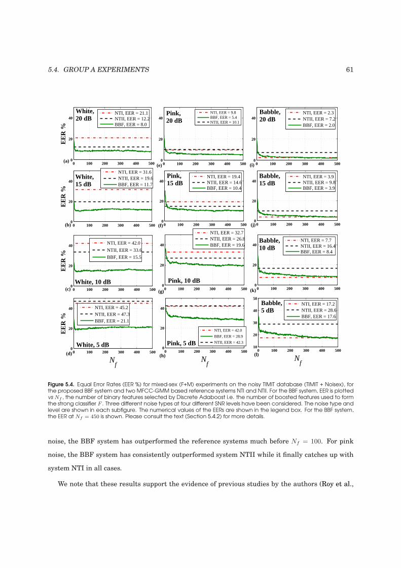
5.4. GROUP A EXPERIMENTS 61
0 100 200 300 400 5000
20
40
EE
R %
0 100 200 300 400 5000
20
40
EE
R %
0 100 200 300 400 5000
20
40
EE
R %
0 100 200 300 400 5000
20
40
Nf
EE
R %
0 100 200 300 400 5000
20
40
0 100 200 300 400 5000
20
40
0 100 200 300 400 5000
20
40
0 100 200 300 400 5000
20
40
Nf
0 100 200 300 400 5000
20
40
0 100 200 300 400 5000
20
40
0 100 200 300 400 5000
20
40
0 100 200 300 400 50010
20
30
40
50
Nf
NTI, EER = 2.3NTII, EER = 7.2BBF, EER = 2.0
NTI, EER = 21.1NTII, EER = 12.2BBF, EER = 8.0
NTI, EER = 31.6NTII, EER = 19.6BBF, EER = 11.7
NTI, EER = 42.0
NTII, EER = 33.6
BBF, EER = 15.5
NTI, EER = 45.2NTII, EER = 47.3BBF, EER = 21.1
NTI, EER = 19.4NTII, EER = 14.6BBF, EER = 10.4
NTI, EER = 32.7NTII, EER = 26.8BBF, EER = 19.6
NTI, EER = 3.9NTII, EER = 9.8BBF, EER = 3.9
NTI, EER = 7.7NTII, EER = 16.4BBF, EER = 8.4
NTI, EER = 17.2NTII, EER = 28.6BBF, EER = 17.6
NTI, EER = 9.8BBF, EER = 5.4NTII, EER = 10.1
NTI, EER = 42.0
BBF, EER = 28.9
NTII, EER = 42.3
White, 15 dB
Pink, 15 dB
Babble, 20 dB
Babble, 15 dB
Babble, 10 dB
Babble, 5 dB
Pink, 20 dB
(a)(e) (i)
(j)(f)(b)
(c) (g) (k)
(l)(h)(d)
Pink, 5 dB
Pink, 10 dBWhite, 10 dB
White, 5 dB
White, 20 dB
Figure 5.4. Equal Error Rates (EER %) for mixed-sex (F+M) experiments on the noisy TIMIT database (TIMIT + Noisex), forthe proposed BBF system and two MFCC-GMM based reference systems NTI and NTII. For the BBF system, EER is plottedvs Nf , the number of binary features selected by Discrete Adaboost i.e. the number of boosted features used to formthe strong classifier F . Three different noise types at four different SNR levels have been considered. The noise type andlevel are shown in each subfigure. The numerical values of the EERs are shown in the legend box. For the BBF system,the EER at Nf = 450 is shown. Please consult the text (Section 5.4.2) for more details.
noise, the BBF system has outperformed the reference systems much before Nf = 100. For pink
noise, the BBF system has consistently outperformed system NTII while it finally catches up with
system NTI in all cases.
We note that these results support the evidence of previous studies by the authors (Roy et al.,

62 CHAPTER 5. APPLICATION TO SPEAKER RECOGNITION
2010) where a similar framework involving boosted binary features performed better than the stan-
dard MFCC-GMM system on speech corrupted by different types of additive noise.
5.4.3 Experiments on speech corrupted by channel noise: mismatched
condition
The aim here was to examine channel effects, more precisely handset transducer effects, on the
performance of the proposed system, compared to a standard MFCC-GMM system.
Database description
The handset TIMIT (HTIMIT) database was chosen for this work (Reynolds, 1997). The
database was constructed by playing a gender-balanced subset of the TIMIT database through a
Sennheiser head-mounted microphone (‘senh’) and 8 telephone headsets: 4 carbon button micro-
phones (‘cb1’-‘cb4’), 4 electret microphones (‘el1’-‘el4’) and one Sony portable microphone (‘pt1’).
In this way, headset transducer degradations were imposed in a systematic way, maintaining the
speaker and linguistic richness of the original TIMIT database. The training and test sentences had
different lexical content, hence this is also an example of text-independent speaker recognition.
Systems evaluated, protocol and experimental details
Apart from the proposed system, the MFCC-GMM system described in Section 5.4.2 (Bimbot
et al., 2004; Yiu et al., 2007) was used as reference. 12 To reduce linear filter effects due to the head-
set transducers, cepstral mean subtraction (CMS) was performed on the MFCC for the reference
system. Similarly, for the BBF system, the spectral magnitude vector X (ref. Section 5.2.1) was
replaced by its log followed by mean normalization.
As in Section 5.4.2, different values of the metaparameters (ie. number of cepstral features,
number of Gaussian mixtures) were tried for the reference system. Among the different configura-
tions tried, we report here two of the best performing ones:
1. Reference system HTI: 16 MFCC, CMS and 32-mixture GMM.
12. In this case also, we implemented the reference system ourselves.
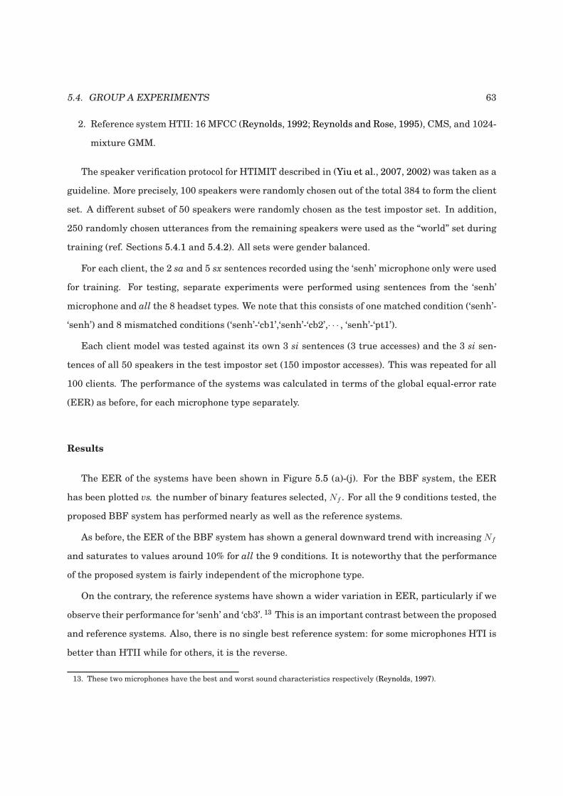
5.4. GROUP A EXPERIMENTS 63
2. Reference system HTII: 16 MFCC (Reynolds, 1992; Reynolds and Rose, 1995), CMS, and 1024-
mixture GMM.
The speaker verification protocol for HTIMIT described in (Yiu et al., 2007, 2002) was taken as a
guideline. More precisely, 100 speakers were randomly chosen out of the total 384 to form the client
set. A different subset of 50 speakers were randomly chosen as the test impostor set. In addition,
250 randomly chosen utterances from the remaining speakers were used as the “world” set during
training (ref. Sections 5.4.1 and 5.4.2). All sets were gender balanced.
For each client, the 2 sa and 5 sx sentences recorded using the ‘senh’ microphone only were used
for training. For testing, separate experiments were performed using sentences from the ‘senh’
microphone and all the 8 headset types. We note that this consists of one matched condition (‘senh’-
‘senh’) and 8 mismatched conditions (‘senh’-‘cb1’,‘senh’-‘cb2’,· · · , ‘senh’-‘pt1’).
Each client model was tested against its own 3 si sentences (3 true accesses) and the 3 si sen-
tences of all 50 speakers in the test impostor set (150 impostor accesses). This was repeated for all
100 clients. The performance of the systems was calculated in terms of the global equal-error rate
(EER) as before, for each microphone type separately.
Results
The EER of the systems have been shown in Figure 5.5 (a)-(j). For the BBF system, the EER
has been plotted vs. the number of binary features selected, Nf . For all the 9 conditions tested, the
proposed BBF system has performed nearly as well as the reference systems.
As before, the EER of the BBF system has shown a general downward trend with increasing Nf
and saturates to values around 10% for all the 9 conditions. It is noteworthy that the performance
of the proposed system is fairly independent of the microphone type.
On the contrary, the reference systems have shown a wider variation in EER, particularly if we
observe their performance for ‘senh’ and ‘cb3’. 13 This is an important contrast between the proposed
and reference systems. Also, there is no single best reference system: for some microphones HTI is
better than HTII while for others, it is the reverse.
13. These two microphones have the best and worst sound characteristics respectively (Reynolds, 1997).
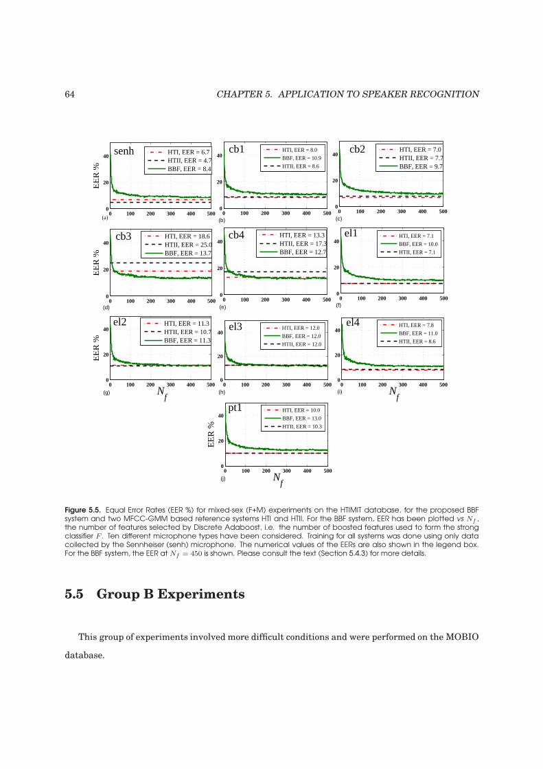
64 CHAPTER 5. APPLICATION TO SPEAKER RECOGNITION
0 100 200 300 400 5000
20
40
EE
R %
0 100 200 300 400 5000
20
40
0 100 200 300 400 5000
20
40
0 100 200 300 400 5000
20
40
EE
R %
0 100 200 300 400 5000
20
40
0 100 200 300 400 5000
20
40
0 100 200 300 400 5000
20
40
Nf
EE
R %
0 100 200 300 400 5000
20
40
0 100 200 300 400 5000
20
40
Nf
0 100 200 300 400 5000
20
40
Nf
EE
R %
HTI, EER = 7.0HTII, EER = 7.7BBF, EER = 9.7
HTI, EER = 6.7HTII, EER = 4.7BBF, EER = 8.4
HTI, EER = 18.6HTII, EER = 25.0BBF, EER = 13.7
HTI, EER = 13.3HTII, EER = 17.3BBF, EER = 12.7
HTI, EER = 11.3HTII, EER = 10.7BBF, EER = 11.3
HTI, EER = 8.0
BBF, EER = 10.9
HTII, EER = 8.6
HTI, EER = 12.0
BBF, EER = 12.0
HTII, EER = 12.0
HTI, EER = 10.0
BBF, EER = 13.0
HTII, EER = 10.3
HTI, EER = 7.1
BBF, EER = 10.0
HTII, EER = 7.1
HTI, EER = 7.8
BBF, EER = 11.0
HTII, EER = 8.6
cb4
pt1
el4
el1
cb1senh
cb3
el2 el3
cb2
(j)
(i)
(f)
(b) (c)(a)
(d)
(g) (h)
(e)
Figure 5.5. Equal Error Rates (EER %) for mixed-sex (F+M) experiments on the HTIMIT database, for the proposed BBFsystem and two MFCC-GMM based reference systems HTI and HTII. For the BBF system, EER has been plotted vs Nf ,the number of features selected by Discrete Adaboost, i.e. the number of boosted features used to form the strongclassifier F . Ten different microphone types have been considered. Training for all systems was done using only datacollected by the Sennheiser (senh) microphone. The numerical values of the EERs are also shown in the legend box.For the BBF system, the EER at Nf = 450 is shown. Please consult the text (Section 5.4.3) for more details.
5.5 Group B Experiments
This group of experiments involved more difficult conditions and were performed on the MOBIO
database.
5.5. GROUP B EXPERIMENTS 65
5.5.1 Database description
The MOBIO Phase I database (Marcel et al., 2010a) consists of speech data collected from 152
people (100 males, 52 females) using a Nokia N93i mobile phone. The data was collected at 6
different sites in 5 different countries. 14 Data for each speaker was collected in 6 separate sessions,
with a gap of at least one month between sessions. There were both native and non-native English
speakers.
In each session, the speakers were asked to answer a set of 21 questions which were classified
as: a) 5 questions requiring 5 short set response answers (read speech from the mobile display), b) 1
question requiring 1 long set response answer (read speech from a paper), and c) 15 questions each
requiring free speech answer. Each answer was recorded as one utterance. The utterances were
short, with a mean duration of 3.5 seconds.
This database was chosen for this group of experiments for the following reasons. Firstly, it
presents a number of challenges, such as:
– The audio data collected on mobile phones had a significant amount of noise (Marcel et al.,
2010b). Figure 5.6 (a) shows the distribution of the utterances according to their SNRs. It is
observed that about 10 % of the utterances had SNRs less than 5 dB, while 60 % had SNRs
between 5 to 10 dB.
– Test utterances were often extremely short, less than 2 seconds in length. Figure 5.6 (b) shows
the distribution of the utterances according to the duration of speech contained in them. It
is observed that about 25 % of utterances had less than 2 seconds of speech, while 35 % had
between 2 to 3 seconds of speech.
– The data presented possibilities for testing different levels of mismatch using a challenging
protocol (Section 5.5.3).
Secondly, it was used for the recent MOBIO Face and Speaker Verification Evaluation contest at
ICPR 2010. 15 Hence, there already exists a large number of reference results from various sites
involving state-of-the-art SV systems. This is useful for comparison.
14. The sites are 1) University of Manchester (UMAN), 2) University of Surrey (UNIS), 3) Idiap Research Institute(IDIAP), 4) Brno University of Technology (BUT), 5) University of Avignon (LIA) and 6) University of Oulu (UOULU).15. www.mobioproject.org/icpr-2010

66 CHAPTER 5. APPLICATION TO SPEAKER RECOGNITION
(a)0−5dB 5−10dB 10−15dB 15−20dB 20−25dB >25dB
0
10
20
30
40
50
60
SNR range
Per
cent
age
of u
ttera
nces
Distribution of utterances according to SNR in the MOBIO Phase Idatabase
(b)0−1 1−2 2−3 3−4 4−5 5−6 6−7 7−8 8−9 9−10
0
10
20
30
40
Amount of speech (seconds)
Per
cent
age
of u
ttera
nces
Distribution of utterances according to amount of speech(in seconds)in the MOBIO Phase Idatabase
Figure 5.6. Distribution of utterances in the MOBIO Phase I database, according to (a) their SNR (dB), (b) amount ofspeech in seconds.
5.5.2 Systems evaluated
The proposed BBF system was compared with 17 state-of-the-art reference systems imple-
mented by five independent research groups, all of which participated in the MOBIO contest at
ICPR 2010 (Marcel et al., 2010b). The reference system details are provided in (Marcel et al.,
2010b,a). Here, we highlight the chief aspects of these reference systems for convenience. Brno
University of Technology (BUT) submitted three speaker verification systems: a) BUT 1, based on
Joint Factor Analysis, b) BUT 2, based on I-vector system, and c) BUT 3, a fusion of these two. They
used 19 MFCC (24 Mel filters) + Energy + 19 ∆MFCC + ∆Energy + 19 ∆∆MFCC + ∆∆ Energy as
features, with short-time Gaussianization using a window of 3 seconds duration. The features were
modelled using a 2048 mixture GMM and 300 eigenvoices and 100 eigenchannels were extracted
for the JFA system. For the I-vector system, they used S-norm for score normalization. In all cases,
the systems were calibrated with Linear Logistic Regression (LLR) to estimate true Log Likelihood
Ratio scores.
The University of Avignon (LIA) submitted two SV systems: a) LIA 1: This used 29 Linear
5.5. GROUP B EXPERIMENTS 67
Frequency Cepstral Coefficients 16 (LFCC) using 50 filters + 29 ∆LFCC + 11 ∆∆ LFCC + ∆ Energy
as features, modelled using 512 mixture GMM. b) LIA 2: This used 19 LFCC (using 24 filters) + 19
∆LFCC + 11 ∆∆ LFCC + ∆ Energy as features, modelled using 256 mixture GMM. Both systems
used feature Gaussianization, Latent Factor Analysis and T-norm.
Tecnologico de Monterrey, Mexico and Arizona State University, USA (TEC-ASU) submitted two
SV systems: a) TEC-ASU 1: This used 16 cepstra + 16 ∆ cepstra + log Energy as features. b) TEC-
ASU 2: This used 16 cepstra + 16∆ cepstra + 16∆∆ cepstra + log Energy as features. Both systems
used 23 channel Mel filterbank for calculation of cepstral features, feature Gaussianization and a
512 mixture GMM-UBM system for modelling the features.
The University of West Bohemia (UWB) submitted 4 SV systems, all using MFCC + ∆MFCC
as features (40-dimensional feature vector) derived from 50 Mel filters, with mean and variance
normalization. The 4 systems are: a) UWB 1: This used GMM-UBM framework with 510 mix-
tures. b) UWB 2: This used Support Vector Machines (SVMs) utilising a GMM Supervector (GSV)
kernel (supervector length = 510 × 40 = 20400. c) UWB 3: This used Support Vector Machines
(SVMs) utilising Generalised Linear Discriminant Sequence (GLDS) kernel with polynomial order
3 (supervector length = 12341). d) UWB 4: This was a fusion of first 3 systems.
Finally, Swansea University and Validsoft (SUV) submitted 3 SV systems: a) SUV 1: It is a
GMM-MAP system whose features are wide band mel frequency cepstral coefficients (MFCCs)
based on 50 Mel filters and 29 cepstral coefficients. b) SUV 2: It is a GMM-MAP system whose
features are wide band MFCCs based on a standard configuration of 24 Mel filters and 16 cepstral
coefficients. c) SUV 3: It is a score level fusion of first two systems after T-normalisation.
Table 5.1 provides a brief summary of the reference systems in terms of feature dimension and
number of Gaussians used.
For the proposed BBF system, precisely the same setup as in previous experiments was used
(Section 5.4.1). No extra processing step was added.
5.5.3 Protocol and experimental details
The SV protocol used was the same as in the MOBIO contest. Details of the protocol are given
in (Marcel et al., 2010a,b). Here, we highlight the chief aspects of this protocol.
16. These are similar to MFCC, except that they are based on the linear frequency scale.

68 CHAPTER 5. APPLICATION TO SPEAKER RECOGNITION
System Feature No. of Gaussiansdimension, ND in the GMM, NG
BUT 1, BUT 2 60 2048
LIA 1, LIA 1a 70 512LIA 2, LIA 2a 50 256
TEC-ASU 1 33 512
TEC-ASU 2 49 512
UWB 1, UWB 2 40 510
SUV 1, SUV 1a 59 512SUV 2 33 512
Table 5.1. Basic parameters of the reference systems, grouped according to submitting institution. Please see Sec-tion 5.5.2 for details.
The database is split into three distinct sets: one for training set, development set and test set.
The data is split so that two sites are used in totality for one set, ie. the three sets are completely
separate with no information regarding individuals or the conditions being shared between any of
the three sets.
The training set could be used in any way deemed appropriate and all of the data was available
for use. Normally the training set would be used to derive background models or an LDA sub-space.
In the case of the proposed approach, the training set was used to derive the negative (‘0’) samples
while boosting each client model in the other two sets.
The development and test sets had their own distinct set of clients. The development set had
to be used to derive a threshold based on the Equal Error Rate (EER) that was then applied to the
test set.
The test set was used to derive the final set of scores. No parameters could be derived from this
set, with only the enrolment data for each client available for use; no knowledge about the other
clients was to be used.
The protocol for enrolling and testing were the same for the development set and the test set.
Only the first session could be used to enrol the user but only the five set response questions could
be used for enrolment. Testing was then conducted on each individual file for sessions two to six
(there are five sessions used for development/ testing) and only the 15 free speech questions were
used for testing.
This led to only five enrolment utterances for each user and 75 test client utterances per client
(15 from each session). When producing imposter scores all the other clients were used, for instance

5.5. GROUP B EXPERIMENTS 69
if in total there were 50 clients then the other 49 clients would perform an imposter attack. The
performance was calculated in terms of the HTER on the test set, based on the threshold calculated
at the EER on the development set. Separate experiments for male and female speakers were
conducted.
Hence, the protocol for MOBIO presents some special challenges in addition to the noisy data
itself. They are summarized below:
– Session variability. Only a single session per speaker could be used to train (enrol) the target
speaker models. Testing was done on the remaining five sessions.
– Lexical mismatch The speech used for enrolment and testing had different lexical content.
Hence, this is a text-independent SV problem.
– Speech-type mismatch. The training (enrolment) was done on read speech only while the
testing was on free speech only.
– No other information from the same site as the target speaker other than the target speaker’s
training data could be used while creating the models.
– Site mismatch. All background (impostor) data allowed for training came from 2 sites while
all impostor data used for testing came from the 4 remaining sites.
5.5.4 Results
The Half Total Error Rate (HTER %) on the test set of the MOBIO database for all the 18
systems have been shown in Figure 5.7. In all cases, the performance of the proposed BBF system
is reasonably good, lying near the mean of the reference systems’ performance.
It is noteworthy that the proposed system achieved reasonable HTERs using only a simple
framework involving a weighted sum of simple binary features, 17 whereas most of the reference
systems used sophisticated techniques involving feature normalization, SVM supervectors, JFA,
LFA and score normalization in addition to the standard MFCC-GMM setup. 18 While such en-
hancements enabled the best reference systems to perform better than the proposed BBF system,
several of the reference systems also performed worse than BBF in spite of their complexity. This
indicates that the BBF system achieves a good trade-off between system performance and complex-
17. For both genders, the BBF system performance saturated around Nf = 100.18. The computational complexities of the proposed and standard reference systems will be analyzed in Section 5.6.2 in
detail.
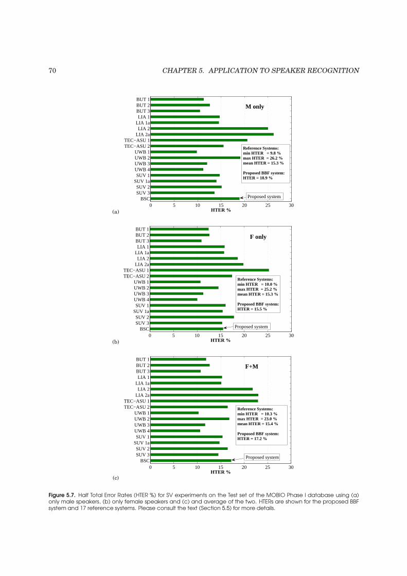
70 CHAPTER 5. APPLICATION TO SPEAKER RECOGNITION
(a)
0 5 10 15 20 25 30
BUT 1BUT 2BUT 3LIA 1
LIA 1aLIA 2
LIA 2aTEC−ASU 1TEC−ASU 2
UWB 1UWB 2UWB 3UWB 4SUV 1
SUV 1aSUV 2SUV 3
BSC
HTER %
M only
Reference Systems:min HTER = 9.8 %max HTER = 26.2 %mean HTER = 15.3 %
Proposed BBF system:HTER = 18.9 %
Proposed system
(b)
0 5 10 15 20 25 30
BUT 1BUT 2BUT 3LIA 1
LIA 1aLIA 2
LIA 2aTEC−ASU 1TEC−ASU 2
UWB 1UWB 2UWB 3UWB 4SUV 1
SUV 1aSUV 2SUV 3
BSC
HTER %
F only
Proposed system
Reference Systems:min HTER = 10.0 %max HTER = 25.2 %mean HTER = 15.3 %
Proposed BBF system:HTER = 15.5 %
(c)
0 5 10 15 20 25 30
BUT 1BUT 2BUT 3LIA 1
LIA 1aLIA 2
LIA 2aTEC−ASU 1TEC−ASU 2
UWB 1UWB 2UWB 3UWB 4SUV 1
SUV 1aSUV 2SUV 3
BSC
HTER %
F+M
Reference Systems:min HTER = 10.3 %max HTER = 23.0 %mean HTER = 15.4 %
Proposed BBF system:HTER = 17.2 %
Proposed system
Figure 5.7. Half Total Error Rates (HTER %) for SV experiments on the Test set of the MOBIO Phase I database using (a)only male speakers, (b) only female speakers and (c) and average of the two. HTERs are shown for the proposed BBFsystem and 17 reference systems. Please consult the text (Section 5.5) for more details.

5.6. ANALYSIS OF THE PROPOSED SYSTEM APPLIED TO SPEAKER RECOGNITION 71
ity.
5.6 Analysis of the proposed system applied to speaker
recognition
From Sections 5.4.1, 5.4.2, 5.4.3 and 5.5.4, we observe that the proposed BBF system shows
comparable text-independent speaker recognition performance vis-a-vis the standard systems (both
baseline and state-of-the-art) across a wide spectrum of conditions, both clean and noisy, matched
and mismatched, using speech either collected using a standard microphone setup or a mobile
phone.
Hence, it seems to fulfill the first objective outlined in Section 5.1, ie. robustness. At the same
time, the proposed system fulfills the second objective, ie. computational efficiency. In the next
two sections, we analyze these two important aspects of the proposed system: a) robustness in the
presence of noise (additive) (Section 5.6.1), and b) computational complexity (Section 5.6.2). In the
final section, we analyse the distribution of the selected binary features in terms of their frequency
locations.
5.6.1 Robustness to additive noise
In Section 5.4.2, it was shown that the BBF system wasmore robust to different types of additive
noise in a mismatched scenario, than the standard MFCC-GMM system. This is an important
property of the BBF system. Here, we provide an analysis of this property at the frame level. 19
For the analysis, we picked out two speakers from the TIMIT database at random. The first
speaker served as the true client, while the second served as an impostor. 20 We had already created
the models for the client (i.e. the strong classifier F for the BBF system and the UBM-GMM for the
MFCC-GMM system) using clean training data. Next, one speech frame from the test data of both
speakers in the TIMIT database was extracted. Three types of noise (white, pink and babble) at 4
different SNRs were subsequently added to these clean speech frames to create noisy speech frames
19. For simplicity, we restrict ourselves to analysis of system behaviour under additive noise in this work. Similar analysescould be carried out for the case of convolutive noise also.20. We shall henceforth denote them as ‘client’ and ‘impostor’ respectively.
72 CHAPTER 5. APPLICATION TO SPEAKER RECOGNITION
(ref. Section 5.4.2). These frames were then passed to the client models and finally the frame scores
were generated.
The process of score generation is depicted in Figure 5.8. In this figure, the left half illustrates
true client accesses, i.e. the client speech frame was matched with the client model, while the right
half illustrates impostor accesses, i.e. the impostor speech framewasmatched with the clientmodel.
The first three rows from the top depict the BBF system while the last two depict the MFCC-GMM
system.
Frame-level behaviour under clean condition
In the first row, subfigures (a) and (c) show the (±1) values of the first 40 boosted binary features
f∗n
40n=1 of the BBF system for the clean speech frames. We note that the binary features have a
value of mostly ‘1’ (light yellow bands) for the client frame and mostly ‘-1’ (dark green bands) for
the impostor frame. The precise number of features with the value ‘1’ is shown in subfigures (e)
and (g) in the second row: a high number for the client and low for the impostor. This is how it
should be: for the client frame, there should be more binary features with a value of ‘1’ so that their
weighted summation is higher, while for the impostor, less features should have a value of ‘1’ so
that their summation is lower. The summation F (X) considering only these first 40 binary features
(ref. Equation 5.2) is shown by the green broken line in subfigures (i1-3), (j1-3).
In the fourth row, subfigures (k) and (m) show the cepstral vectors XM extracted from the clean
speech frames for the MFCC-GMM system. The loglikelihood ratio scores (LLR) obtained by passing
these vectors through the UBM-GMM of the client is shown by green broken line in subfigures (o1-
3), (p1-3).
For both the BBF and MFCC-GMM systems, we see that the client and impostor scores are well
separated in the clean condition.
Frame-level behaviour under noisy condition
In the case of the BBF system, as different types of noise are added at different SNRs to the
clean test frame, the binary feature values vary due to the change in the shape of the spectrum.
These variations ∆(f∗n)
40n=1 are shown in subfigures (b1-3), (d1-3). The most important point to
note is that a significant number of binary feature values remain unchanged after noise addition,
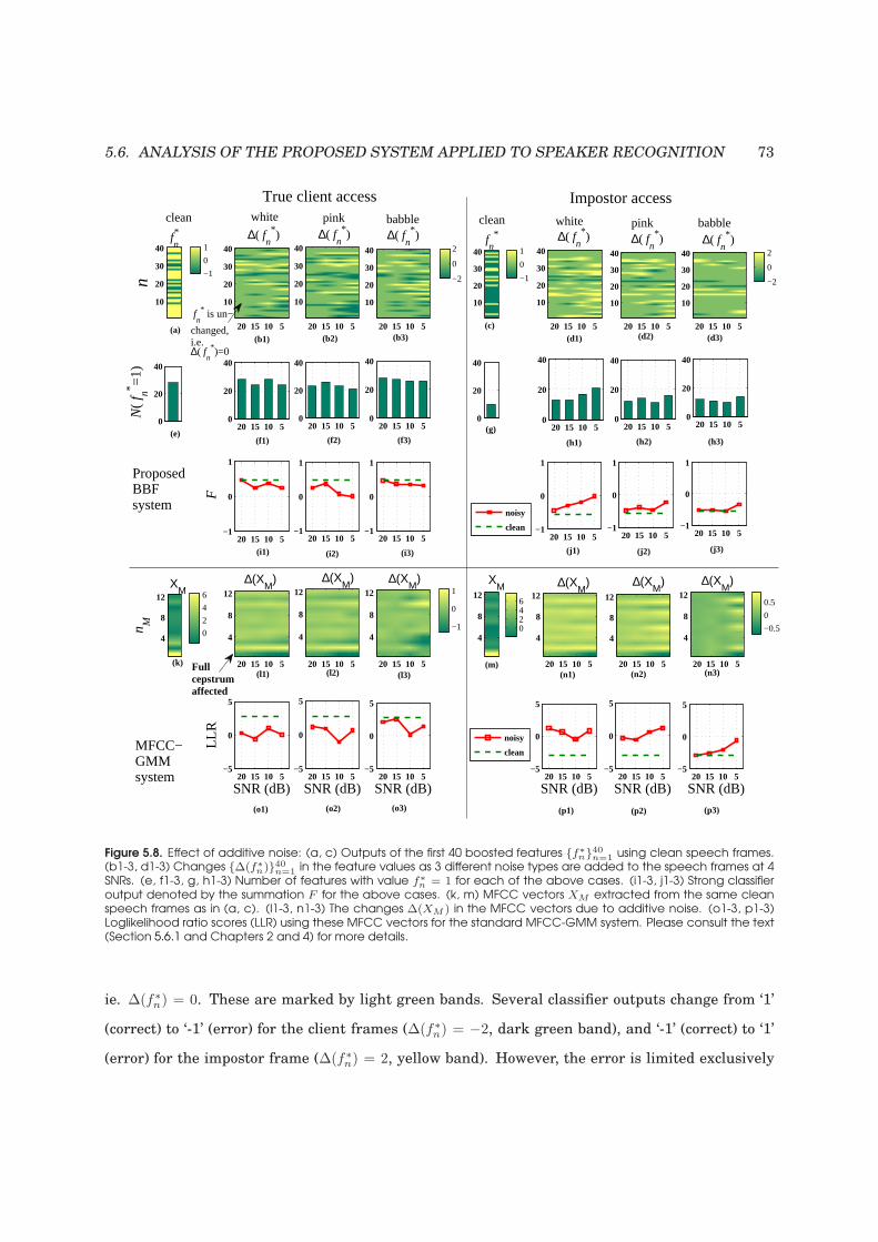
5.6. ANALYSIS OF THE PROPOSED SYSTEM APPLIED TO SPEAKER RECOGNITION 73n
10
20
30
40
0
20
40
N(
f n* =1)
n M
4
8
12
20 15 10 5
10
20
30
40
20 15 10 50
20
40
20 15 10 5−1
0
1
F
20 15 10 5
4
8
12
20 15 10 5−5
0
5
SNR (dB)
LLR
20 15 10 5
10
20
30
40
20 15 10 50
20
40
20 15 10 5−1
0
1
20 15 10 5
4
8
12
20 15 10 5−5
0
5
SNR (dB)
20 15 10 5
10
20
30
40
20 15 10 50
20
40
20 15 10 5−1
0
1
20 15 10 5
4
8
12
20 15 10 5−5
0
5
SNR (dB)
10
20
30
40
0
20
40
4
8
12
20 15 10 5
10
20
30
40
20 15 10 50
20
40
20 15 10 5−1
0
1
20 15 10 5
4
8
12
20 15 10 5−5
0
5
SNR (dB)
20 15 10 5
10
20
30
40
20 15 10 50
20
40
20 15 10 5−1
0
1
20 15 10 5
4
8
12
20 15 10 5−5
0
5
SNR (dB)
20 15 10 5
10
20
30
40
20 15 10 50
20
40
20 15 10 5−1
0
1
20 15 10 5
4
8
12
20 15 10 5−5
0
5
SNR (dB)
−1
0
1
−2
0
2
−1
0
1
−2
0
2
0
2
4
6
−1
0
1
0246
−0.5
0
0.5
noisy
clean
noisy
clean
(c)
(k) (m)
(b1) (b2) (b3)(a)
(f1) (f2) (f3)
(i1) (i2) (i3)
(g)(e)(h1) (h2) (h3)
(j3)(j2)(j1)
(d3)(d1) (d2)
(l1) (l2) (l3) (n1) (n2) (n3)
(o1) (o2) (o3) (p1) (p2) (p3)
True client accesswhite pink babble
MFCC−GMMsystem
XM
Impostor access
babblepinkwhitecleanclean
ProposedBBFsystem
∆( fn*)∆( f
n*) ∆( f
n*)
fn* is un−
changed,i.e.∆( f
n*)=0
∆( fn*)
∆(XM
) ∆(XM
) ∆(XM
)∆(XM
)∆(XM
)∆(XM
)
Fullcepstrumaffected
fn* ∆( f
n*) ∆( f
n*) f
n*
XM
Figure 5.8. Effect of additive noise: (a, c) Outputs of the first 40 boosted features f∗
n40n=1
using clean speech frames.(b1-3, d1-3) Changes ∆(f∗
n)40n=1
in the feature values as 3 different noise types are added to the speech frames at 4SNRs. (e, f1-3, g, h1-3) Number of features with value f∗
n = 1 for each of the above cases. (i1-3, j1-3) Strong classifieroutput denoted by the summation F for the above cases. (k, m) MFCC vectors XM extracted from the same cleanspeech frames as in (a, c). (l1-3, n1-3) The changes ∆(XM ) in the MFCC vectors due to additive noise. (o1-3, p1-3)Loglikelihood ratio scores (LLR) using these MFCC vectors for the standard MFCC-GMM system. Please consult the text(Section 5.6.1 and Chapters 2 and 4) for more details.
ie. ∆(f∗n) = 0. These are marked by light green bands. Several classifier outputs change from ‘1’
(correct) to ‘-1’ (error) for the client frames (∆(f∗n) = −2, dark green band), and ‘-1’ (correct) to ‘1’
(error) for the impostor frame (∆(f∗n) = 2, yellow band). However, the error is limited exclusively
74 CHAPTER 5. APPLICATION TO SPEAKER RECOGNITION
to these outputs. Interestingly, some erroneous outputs become correct too (∆(f∗n) = 2 for the client
and ∆(f∗n) = −2 for the impostor). 21
The number of binary features with the value ‘1’ is again shown in subfigures (f1-3), (h1-3)
and the final scores F (X) are shown by the red lines in subfigures (i1-3), (j1-3). We note that the
client and impostor scores have approached each other gradually, as the SNR has reduced. This is
expected.
Similarly, in the case of the standard MFCC-GMM SV system, as different types of noise are
added to the clean test frame, the cepstral vectors XM change values. These changes ∆(XM ) are
shown in subfigures (l1-3), (n1-3). 22 Contrary to the BBF system where the error is limited to
certain binary features, we note that the entire cepstrum has been distorted by noise, even when
the SNR is high. Some cepstral coefficients will be affected more and some affected less. The
loglikelihood ratio scores obtained by passing these noisy vectors through the UBM-GMM of the
client is shown by the red lines in subfigures (o1-3), (p1-3).
We observe that for each noise type and SNR level, the client and impostor scores have ap-
proached each other less in the BBF system (in terms of the summation F (X)) than in the MFCC-
GMM system (in terms of the loglikelihood ratios). This would lead to better separability and lower
verification errors for the BBF system.
This could be mainly due to the fact that although the noise did affect some of the binary fea-
tures, it could not affect a large fraction of these features. These correct features could combine
together and offset the effect of the incorrect ones. In MFCC-GMM system, the entire cepstrum is
affected and we cannot avail of this unique advantage. This is a characteristic of the localized or
parts-based approach. In addition, since the binary features involve a thresholding operation, the
system is unaffected by noise as long as it is does not cross the threshold. This advantage is also
unique to the binary features. The cepstral features will be immediately affected even if there is a
small amount of noise.
21. Due to the fact that Adaboost looks at each binary feature as a “weak classifier”, we consider that a binary featurefrom a client frame should ideally have a value of ‘1’ while one from an impostor frame should have a value of ‘-1’. If thishappens, the features are considered to have a correct value. Otherwise, it is an error and the features have an incorrectvalue. In practice, this does not happen and is also not necessary.22. The same noisy frame was used for both the BBF and MFCC-GMM systems, for all cases.
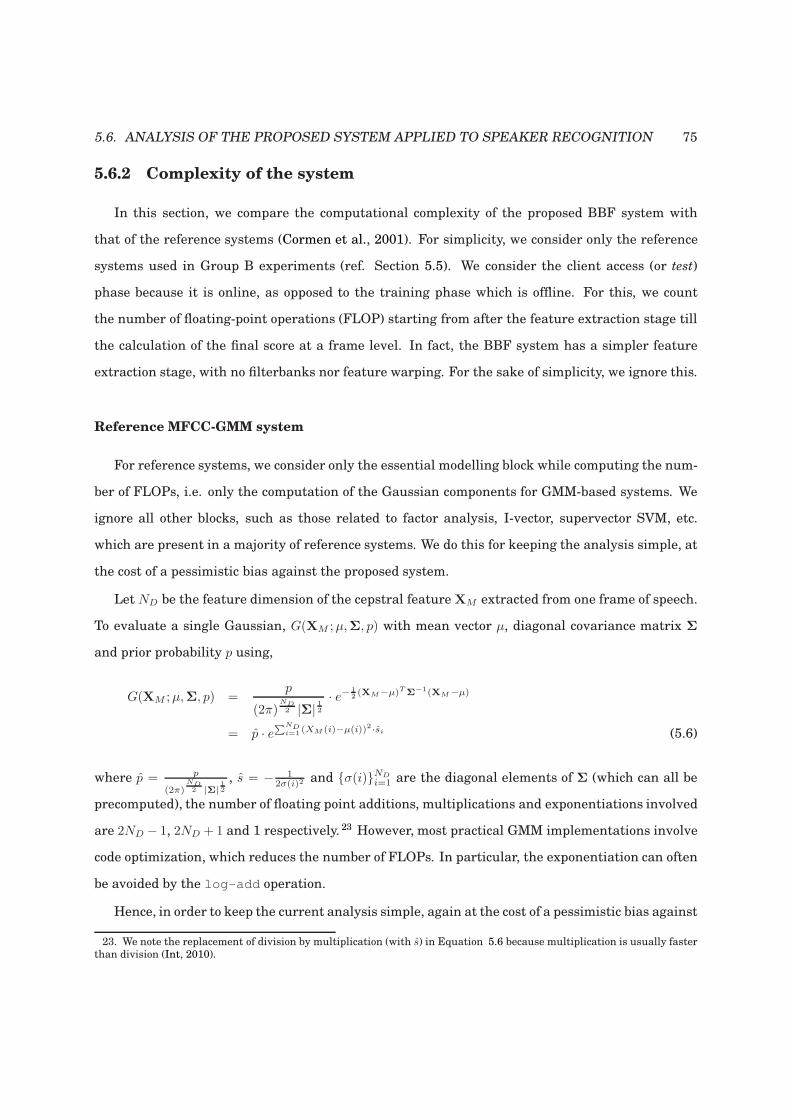
5.6. ANALYSIS OF THE PROPOSED SYSTEM APPLIED TO SPEAKER RECOGNITION 75
5.6.2 Complexity of the system
In this section, we compare the computational complexity of the proposed BBF system with
that of the reference systems (Cormen et al., 2001). For simplicity, we consider only the reference
systems used in Group B experiments (ref. Section 5.5). We consider the client access (or test)
phase because it is online, as opposed to the training phase which is offline. For this, we count
the number of floating-point operations (FLOP) starting from after the feature extraction stage till
the calculation of the final score at a frame level. In fact, the BBF system has a simpler feature
extraction stage, with no filterbanks nor feature warping. For the sake of simplicity, we ignore this.
Reference MFCC-GMM system
For reference systems, we consider only the essential modelling block while computing the num-
ber of FLOPs, i.e. only the computation of the Gaussian components for GMM-based systems. We
ignore all other blocks, such as those related to factor analysis, I-vector, supervector SVM, etc.
which are present in a majority of reference systems. We do this for keeping the analysis simple, at
the cost of a pessimistic bias against the proposed system.
Let ND be the feature dimension of the cepstral featureXM extracted from one frame of speech.
To evaluate a single Gaussian, G(XM ;µ,Σ, p) with mean vector µ, diagonal covariance matrix Σ
and prior probability p using,
G(XM ;µ,Σ, p) =p
(2π)ND2 |Σ|
12
· e−12 (XM−µ)TΣ
−1(XM−µ)
= p · e∑ND
i=1(XM (i)−µ(i))2·si (5.6)
where p = p
(2π)ND2 |Σ|
12
, s = − 12σ(i)2 and σ(i)ND
i=1 are the diagonal elements of Σ (which can all be
precomputed), the number of floating point additions, multiplications and exponentiations involved
are 2ND − 1, 2ND + 1 and 1 respectively. 23 However, most practical GMM implementations involve
code optimization, which reduces the number of FLOPs. In particular, the exponentiation can often
be avoided by the log-add operation.
Hence, in order to keep the current analysis simple, again at the cost of a pessimistic bias against
23. We note the replacement of division by multiplication (with s) in Equation 5.6 because multiplication is usually fasterthan division (Int, 2010).
76 CHAPTER 5. APPLICATION TO SPEAKER RECOGNITION
the proposed system, we only consider the computation of the quadratic term (XM −µ)TΣ−1(XM −
µ) ≡∑ND
i=1(XM (i)− µ(i))2 · si in Eq. 5.6. This term must be computed once per Gaussian, indepen-
dent of the level of optimization achieved. To compute it, 2ND floating point multiplications and
2ND − 1 floating point additions are required. Hence, to process one frame of speech, we multiply
these quantities by NG, the number of Gaussians. Thus, the total number of multiplications and
additions per frame is, n× = 2NGND, n+ = NG(2ND − 1) respectively. Hence, the total number of
FLOPs per frame is:
NFLOP = n× + n+ = NG(4ND − 1). (5.7)
Proposed BBF system
Let X be a spectral vector extracted from a speech frame (ref. Section 5.2.1).
Let Nf be the number of boosted binary features used to form the strong clas-
sifier F (ref. Section 5.2.2). To obtain the final frame-level score F (X), we
must use Equations 5.1 and 5.2 which we combine and implement as follows:
F (X)← 0
for n = 1 to Nf
a← 0 , αn
b← (X(kn,1)−X(kn,2) ≥ θn)
F (X)← F (X) + a[b]
end
Here, a[b] denotes the b-th element of array a. Since they usually take almost the same time (Int,
2010), we group the number of comparisons, additions and subtractions as n+. From the above
implementation, we find that for the BBF system, no multiplication is required and,
NFLOP = n+ = 3Nf (5.8)
5.6. ANALYSIS OF THE PROPOSED SYSTEM APPLIED TO SPEAKER RECOGNITION 77
102
103
104
105
106
BUT 1BUT 2BUT 3LIA 1
LIA 1aLIA 2
LIA 2aTEC−ASU 1TEC−ASU 2
UWB 1UWB 2UWB 3UWB 4SUV 1
SUV 1aSUV 2SUV 3
BSC
NFLOP
Reference Systems:min N
FLOP = 1.2 × 10⁴
max NFLOP
= 7.4 × 10⁵
mean NFLOP
= 1.5 × 10⁵
Proposed BBF system:N
FLOP = 300
Proposed system
Figure 5.9. Number of floating-point operations, NFLOP plotted in log-scale, for the 17 reference systems used in theGroup B experiments and the proposed BBF system. Please see text (Section 5.6.2) for more details.
The total number of FLOPs for BBF and reference systems calculated using Eqns. 5.7 & 5.8 are
shown in Figure 5.9. Parameter values for ND, NG in Equation 5.7 are enlisted in Table 5.1. In
Equation 5.8, parameter Nf = 100. 24
It is observed from Figure 5.9 that BBF system requires a few hundred FLOPs, significantly
less than that required by reference systems (104 − 105 FLOPs). Hence, even with a pessimistic
bias, BBF system is shown to be computationally more efficient. This is an important advantage
of the BBF system particularly with respect to the computational constraints for mobile phone SV
systems (Section 5.1).
5.6.3 Analysis of selected binary features
The total number of binary features in the complete set Φ isNΦ = NF (NF−1) (ref. Section 5.2.1).
In all experiments, we used a fixed value of NF = 128 (ref. Section 5.4.1). Thus, there were NL =
128(128− 1) = 16256 unique binary features, out of which Nf were selected by Adaboost. Here we
aim to find if there are any salient characteristics of these selected binary features.
24. This is average value at which the BBF system reached best performance (Section 5.5.4) for the Group B experiments.
78 CHAPTER 5. APPLICATION TO SPEAKER RECOGNITION
Let us define a matrix A = ai,ji=Nf ,j=Nf
i=1,j=1 defined as
ai,j = EF (αi,j,F ) (5.9)
where
αi,j,F =
Nf∑
n=1
αn · 1kn,1=i ∧ kn,2=j (5.10)
given a particular client model F , and
EF (αi,j,F ) =1
Nc
Nc∑
c=1
αi,j,Fc(5.11)
i.e. the expected value of αi,j,F considering all client models F . Here, a client model is the strong
classifier F corresponding to that client (ref. Section 5.2.2), αn is the weight assigned to the n-th
selected binary feature in F , and Nc is the total number of clients.
Thus, each element ai,j measures the expected total weight assigned to the selected binary
features defined by the frequency indices kn,1 = i, kn,2 = j, over all clients. In other words, a higher
value of ai,j would mean a more informative or discriminative binary feature (and hence, more
informative frequency bins), as determined by Adaboost.
In Figure 5.10, we show the matrix A calculated using the TIMIT database, with the number of
clients Nc = 168. We have indicated the frequencies corresponding to the k values using a sampling
frequency of fs = 16kHz. Higher values of ai,j are marked in yellow and lighter shades of green
and lower values in darker shades of green. We observe that certain regions have distinctly higher
expected weights than others. In particular, values of kn,1, kn,2 ≤ 1kHz seem to be given higher
weights. Also, pairs kn,1, kn,2 with kn,1 close to kn,2 were given higher weights. We analyse these
phenomena in more detail in Figure 5.11. Let us define P (k) as the probability that a binary
feature selected by Adaboost will be parameterized by the frequency point k. We estimate P (k) by
counting over all client models. In Figure 5.11(a), we have plotted the probability P (k) vs. kn,1 and
kn,2. Note that P (k) is plotted in the log-scale. We observe that values of k ≤ 1 kHz seem to be
chosen more often. There is a valley between 1kHz and 2.5kHz followed by a wide plateau. This
seems to correlate with previous studies based on subbands which show that low-frequency and
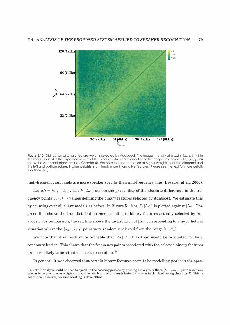
5.6. ANALYSIS OF THE PROPOSED SYSTEM APPLIED TO SPEAKER RECOGNITION 79
kn,1
kn
,2
32 (2kHz) 64 (4kHz) 96 (6kHz) 128 (8kHz)
32 (2kHz)
64 (4kHz)
96 (6kHz)
128 (8kHz)
0.001
0.01
0.1
Figure 5.10. Distribution of binary feature weights selected by Adaboost: The image intensity at a point kn,1, kn,2 inthe image indicates the expected weight of the binary feature corresponding to the frequency indices kn,1, kn,2, asset by the Adaboost algorithm (ref. Chapter 4). We note the concentration of higher weights near the diagonal andthe left and bottom edges. Higher weights might imply more informative features. Please see the text for more details(Section 5.6.3).
high-frequency subbands are more speaker specific than mid-frequency ones (Besacier et al., 2000).
Let ∆k = kn,1 − kn,2. Let P (|∆k|) denote the probability of the absolute differences in the fre-
quency points kn,1, kn,2 values defining the binary features selected by Adaboost. We estimate this
by counting over all client models as before. In Figure 5.11(b), P (|∆k|) is plotted against |∆k|. The
green line shows the true distribution corresponding to binary features actually selected by Ad-
aboost. For comparison, the red line shows the distribution of |∆k| corresponding to a hypothetical
situation where the kn,1, kn,2 pairs were randomly selected from the range [1 : NX].
We note that it is much more probable that |∆k| ≤ 1kHz than would be accounted for by a
random selection. This shows that the frequency points associated with the selected binary features
are more likely to be situated close to each other. 25
In general, it was observed that certain binary features seem to be modelling peaks in the spec-
25. This analysis could be used to speed up the boosting process by pruning out a priori those kn,1, kn,2 pairs which areknown to be given lower weights, since they are less likely to contribute to the sum in the final strong classifier F . This isnot critical, however, because boosting is done offline.
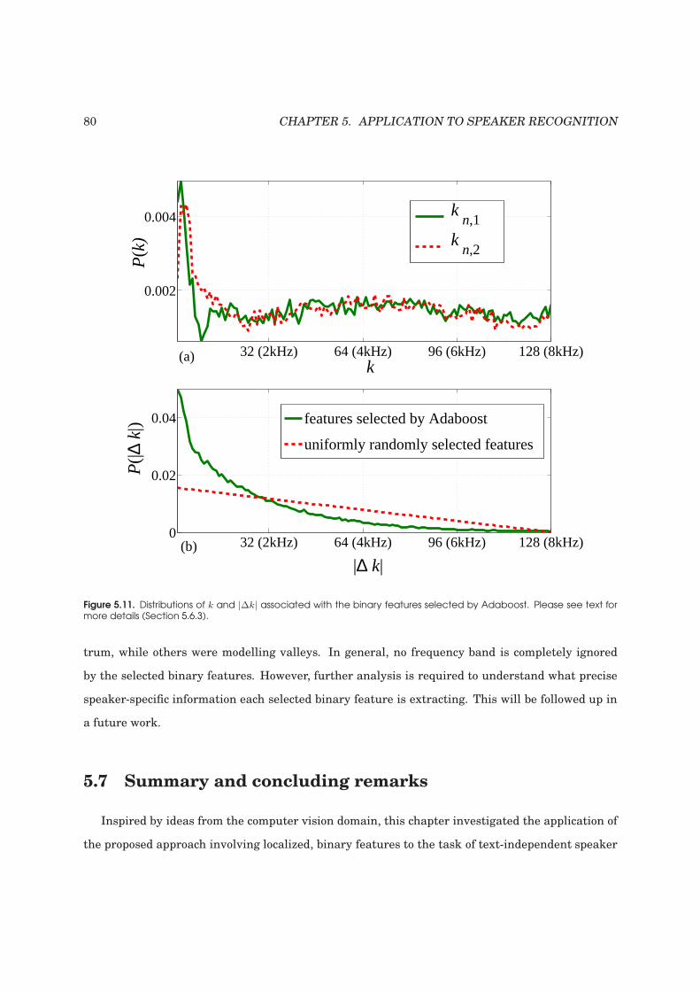
80 CHAPTER 5. APPLICATION TO SPEAKER RECOGNITION
32 (2kHz) 64 (4kHz) 96 (6kHz) 128 (8kHz)
0.002
0.004
k
P(k
)
32 (2kHz) 64 (4kHz) 96 (6kHz) 128 (8kHz)0
0.02
0.04
|∆ k|
P(|∆
k|)
k n,1
k n,2
features selected by Adaboost
uniformly randomly selected features
(a)
(b)
Figure 5.11. Distributions of k and |∆k| associated with the binary features selected by Adaboost. Please see text formore details (Section 5.6.3).
trum, while others were modelling valleys. In general, no frequency band is completely ignored
by the selected binary features. However, further analysis is required to understand what precise
speaker-specific information each selected binary feature is extracting. This will be followed up in
a future work.
5.7 Summary and concluding remarks
Inspired by ideas from the computer vision domain, this chapter investigated the application of
the proposed approach involving localized, binary features to the task of text-independent speaker
5.7. SUMMARY AND CONCLUDING REMARKS 81
recognition. The proposed approach was compared against standard (holistic) cepstral feature-
based approach using baseline and state-of-the-art techniques on several databases, including
TIMIT, noisy TIMIT, HTIMIT and MOBIO.
Our studies showed that the proposed approach yields similar speaker recognition performance
in clean condition and often better performance in noisy conditions when compared to the standard
holistic approach. This observation is similar to what has been observed in the vision and speech
domain for other localized approaches.
Furthermore, the proposed approach involves lower computational complexity compared to the
standard approach. Hence, it seems to fulfill the two objectives related to implementation of speaker
recognition systems on portable devices such as mobile phones, i.e. robustness and computational
efficiency.

82 CHAPTER 5. APPLICATION TO SPEAKER RECOGNITION
Chapter 6
Application of proposed approach
to Automatic Speech Recognition
In this chapter, we present the application of the proposed Boosted Binary Features approach
to the task of automatic speech recognition (ASR). We describe how the generic system described
in Chapter 4 is adapted specifically for the ASR task. In order to evaluate the performance of
the system, several experimental studies are reported. Preliminary experiments involve a simple
phoneme recognition task, i.e. decoding an utterance in terms of its phoneme sequence. Further
experiments involve a continuous speech recognition task, i.e. decoding an utterance in terms
of the word sequence. Fusion of the proposed BBF approach with standard cepstral features is
also studied. The chapter finishes with a discussion of certain interesting aspects of the proposed
system.
6.1 Objectives and motivations
The good performance of the proposed BBF approach on the speaker recognition task as reported
in Chapter 5 motivated us to apply the same approach to ASR. This was possible because the
proposed approach is generic and not linked to a particular task. In the case of speaker recognition,
the Adaboost-based feature selection process was provided with training samples labeled as ‘client’
or ‘impostor’. In the case of ASR, the training samples were labeled with the different phonemes.
83
84 CHAPTER 6. APPLICATION TO AUTOMATIC SPEECH RECOGNITION
The main objective of this work was to apply BBF to the ASR task and present a working ASR
system comparable to the standard cepstral features-based system. To recapitulate, standard ASR
systems primarily use cepstral features which tend to capture the envelop of short-term magnitude
spectrum of speech (ref. Chapter 2, Section 2.1). Dynamic information is subsequently added by
appending approximate temporal derivatives of the cepstral features. These features are holistic,
real-valued and based on prior knowledge. In contrast, the BBF approach for ASR as described in
this chapter involves localized, binary-valued and data-driven features.
Note that the objectives of robustness to noise and computational efficiency mentioned in Chap-
ter 5 are not emphasized in this work. 1 This is because there were other issues particular to the
ASR task which had to be first resolved, as described in the next section.
6.2 Proposed BBF approach applied to Automatic Speech
Recognition (ASR)
It is possible to apply the proposed approach as described in Chapter 4 directly to the ASR task
by considering individual words or phonemes as classes. However, this simple approach does not
give good results. This is because, compared to speaker recognition, ASR is more complicated in
the sense that a decoded ordered sequence of words are required from an utterance, instead of a
single speaker class (client or impostor). Therefore, a sequence modeling framework such as Hidden
Markov Model (HMM) and the associated decoding strategy (Viterbi decoding) are necessary, as
mentioned in the description of standard ASR systems in Chapter 2.
Hence, the first question is how to integrate the proposed BBF approach into an HMM-based
ASR system. For this purpose, we decided to use the BBF framework solely as a data-driven feature
extractor for ASR (Roy et al., 2011b,d). The modeling and decision-making modules described in
Chapter 4 exist here but in a hidden way only to drive the feature selection process. The actual
modeling is done by single layer perceptrons (SLP) or multilayer perceptrons (MLP) (Bourlard and
Morgan, 1994). The temporal sequence is modeled using Kullback Leibler divergence-basedHidden
Markov Model (KL-HMM) (Aradilla, 2008), a variant of the HMM frameworkmentioned in Chapter
1. However, there is significant evidence of robustness to noise in existing localized systems for ASR as mentioned inChapter 3, Section 3.4 and it could be verified if the BBF system also has this characteristic as a part of future work.
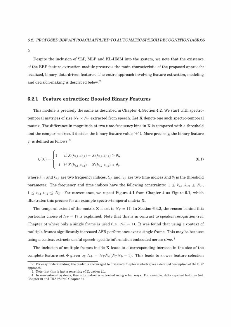
6.2. PROPOSED BBFAPPROACHAPPLIED TO AUTOMATIC SPEECHRECOGNITION (ASR)85
2.
Despite the inclusion of SLP, MLP and KL-HMM into the system, we note that the existence
of the BBF feature extraction module preserves the main characteristic of the proposed approach:
localized, binary, data-driven features. The entire approach involving feature extraction, modeling
and decision-making is described below. 2
6.2.1 Feature extraction: Boosted Binary Features
This module is precisely the same as described in Chapter 4, Section 4.2. We start with spectro-
temporal matrices of size NF ×NT extracted from speech. Let X denote one such spectro-temporal
matrix. The difference in magnitude at two time-frequency bins in X is compared with a threshold
and the comparison result decides the binary feature value (±1). More precisely, the binary feature
fi is defined as follows: 3
fi(X) =
1 if X(ki,1, ti,1)−X(ki,2, ti,2) ≥ θi,
−1 if X(ki,1, ti,1)−X(ki,2, ti,2) < θi.
(6.1)
where ki,1 and ki,2 are two frequency indices, ti,1 and ti,2 are two time indices and θi is the threshold
parameter. The frequency and time indices have the following constraints: 1 ≤ ki,1, ki,2 ≤ NF ,
1 ≤ ti,1, ti,2 ≤ NT . For convenience, we repeat Figure 4.1 from Chapter 4 as Figure 6.1, which
illustrates this process for an example spectro-temporal matrix X.
The temporal extent of the matrix X is set to NT = 17. In Section 6.4.2, the reason behind this
particular choice of NT = 17 is explained. Note that this is in contrast to speaker recognition (ref.
Chapter 5) where only a single frame is used (i.e. NT = 1). It was found that using a context of
multiple frames significantly increased ASR performance over a single frame. This may be because
using a context extracts useful speech-specific information embedded across time. 4
The inclusion of multiple frames inside X leads to a corresponding increase in the size of the
complete feature set Φ given by NΦ = NTNΦ(NTNΦ − 1). This leads to slower feature selection
2. For easy understanding, the reader is encouraged to first read Chapter 4 which gives a detailed description of the BBFapproach.
3. Note that this is just a rewriting of Equation 4.1.4. In conventional systems, this information is extracted using other ways. For example, delta cepstral features (ref.
Chapter 2) and TRAPS (ref. Chapter 3).

86 CHAPTER 6. APPLICATION TO AUTOMATIC SPEECH RECOGNITION
Time index
Fre
quen
cy(M
elfilt
er)
index
Spectro-temporal matrix X
2 4 6 8 10 12 14 16
5
10
15
20
Σ
+1
-1-1
+1
θi
ti,1 = 11ti,2 = 3
X(ki,1, ti,1)
ki,2 = 6
ki,1 = 22
X(ki,2, ti,2)
Binaryfeature
Figure 6.1. Each binary feature fi is associated with a pair of time-frequency bins in the spectro-temporal matrix,defined by the parameters (ki,1, ti,1) and (ki,2, ti,2). The difference of the magnitude at these two bins is comparedwith a threshold θi and the sign is retained. Calculation of an example feature fi is shown in the figure.
during boosting because each boosting iteration involves a loop through all the features in Φ (ref.
Section 4.4). Although the selection stage is offline, we chose to use 24-band Mel spectra instead of
Fourier spectra so that NT is reduced from 128 to 24, leading to faster selection. Hence, the total
number of features NΦ = 24 · 17 · (24 · 17 − 1) = 166056. Another important aspect is that we used
log Mel spectra instead of directly the Mel bank energies, following the standard approach. It was
found that using log energies slightly improved performance.
In the description of the proposed approach in Chapter 4, the feature extraction module was
followed by the modeling module. This module involved the weighted linear summation F of the
binary features (ref. Equation 4.2). Minimization of the exponential loss Lexp,F associated with this
summation acting F as a classifier led to the selection of the most discriminative features via the
Discrete Adaboost algorithm.
Now in the case of ASR, the situation is different. The actual modeling does not involve the
summation F . However, we consider this simple model as a mathematical basis to motivate the
feature selection process, i.e. the features are still selected via the Discrete Adaboost algorithm to
minimize the loss Lexp,F associated with the summation F . Although the actual modeling does not
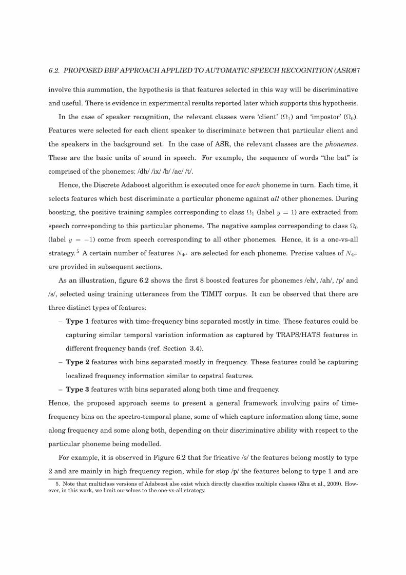
6.2. PROPOSED BBFAPPROACHAPPLIED TO AUTOMATIC SPEECHRECOGNITION (ASR)87
involve this summation, the hypothesis is that features selected in this way will be discriminative
and useful. There is evidence in experimental results reported later which supports this hypothesis.
In the case of speaker recognition, the relevant classes were ‘client’ (Ω1) and ‘impostor’ (Ω0).
Features were selected for each client speaker to discriminate between that particular client and
the speakers in the background set. In the case of ASR, the relevant classes are the phonemes.
These are the basic units of sound in speech. For example, the sequence of words “the bat” is
comprised of the phonemes: /dh/ /ix/ /b/ /ae/ /t/.
Hence, the Discrete Adaboost algorithm is executed once for each phoneme in turn. Each time, it
selects features which best discriminate a particular phoneme against all other phonemes. During
boosting, the positive training samples corresponding to class Ω1 (label y = 1) are extracted from
speech corresponding to this particular phoneme. The negative samples corresponding to class Ω0
(label y = −1) come from speech corresponding to all other phonemes. Hence, it is a one-vs-all
strategy. 5 A certain number of features NΦ∗ are selected for each phoneme. Precise values of NΦ∗
are provided in subsequent sections.
As an illustration, figure 6.2 shows the first 8 boosted features for phonemes /eh/, /ah/, /p/ and
/s/, selected using training utterances from the TIMIT corpus. It can be observed that there are
three distinct types of features:
– Type 1 features with time-frequency bins separated mostly in time. These features could be
capturing similar temporal variation information as captured by TRAPS/HATS features in
different frequency bands (ref. Section 3.4).
– Type 2 features with bins separated mostly in frequency. These features could be capturing
localized frequency information similar to cepstral features.
– Type 3 features with bins separated along both time and frequency.
Hence, the proposed approach seems to present a general framework involving pairs of time-
frequency bins on the spectro-temporal plane, some of which capture information along time, some
along frequency and some along both, depending on their discriminative ability with respect to the
particular phoneme being modelled.
For example, it is observed in Figure 6.2 that for fricative /s/ the features belong mostly to type
2 and are mainly in high frequency region, while for stop /p/ the features belong to type 1 and are
5. Note that multiclass versions of Adaboost also exist which directly classifies multiple classes (Zhu et al., 2009). How-ever, in this work, we limit ourselves to the one-vs-all strategy.
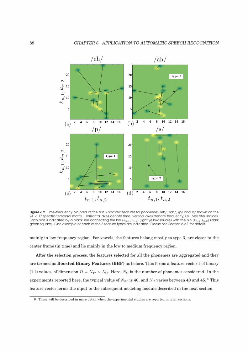
88 CHAPTER 6. APPLICATION TO AUTOMATIC SPEECH RECOGNITION
kn
,1,k
n,2
/eh/
2 4 6 8 10 12 14 16
5
10
15
20
/ah/
2 4 6 8 10 12 14 16
5
10
15
20
tn,1, tn,2
kn
,1,k
n,2
/p/
2 4 6 8 10 12 14 16
5
10
15
20
tn,1, tn,2
/s/
2 4 6 8 10 12 14 16
5
10
15
20
(a) (b)
(c) (d)
type 3
type 1
type 2
Figure 6.2. Time-frequency bin pairs of the first 8 boosted features for phonemes /eh/, /ah/, /p/ and /s/ shown on the24 × 17 spectro-temporal matrix. Horizontal axes denote time, vertical axes denote frequency, i.e. Mel filter indices.Each pair is indicated by a black line connecting the bin (kn,1, tn,1) (light yellow square) with the bin (kn,2, tn,2) (darkgreen square). One example of each of the 3 feature types are indicated. Please see Section 6.2.1 for details.
mainly in low frequency region. For vowels, the features belong mostly to type 3, are closer to the
center frame (in time) and lie mainly in the low to medium frequency region.
After the selection process, the features selected for all the phonemes are aggregated and they
are termed as Boosted Binary Features (BBF) as before. This forms a feature vector f of binary
(±1) values, of dimension D = NΦ∗ ×NΩ. Here, NΩ is the number of phonemes considered. In the
experiments reported here, the typical value of NΦ∗ is 40, and NΩ varies between 40 and 45. 6 This
feature vector forms the input to the subsequent modeling module described in the next section.
6. These will be described in more detail when the experimental studies are reported in later sections.
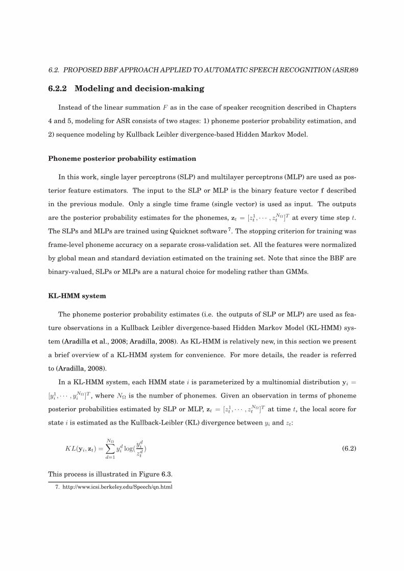
6.2. PROPOSED BBFAPPROACHAPPLIED TO AUTOMATIC SPEECHRECOGNITION (ASR)89
6.2.2 Modeling and decision-making
Instead of the linear summation F as in the case of speaker recognition described in Chapters
4 and 5, modeling for ASR consists of two stages: 1) phoneme posterior probability estimation, and
2) sequence modeling by Kullback Leibler divergence-based Hidden Markov Model.
Phoneme posterior probability estimation
In this work, single layer perceptrons (SLP) and multilayer perceptrons (MLP) are used as pos-
terior feature estimators. The input to the SLP or MLP is the binary feature vector f described
in the previous module. Only a single time frame (single vector) is used as input. The outputs
are the posterior probability estimates for the phonemes, zt = [z1t , · · · , zNΩt ]T at every time step t.
The SLPs and MLPs are trained using Quicknet software 7. The stopping criterion for training was
frame-level phoneme accuracy on a separate cross-validation set. All the features were normalized
by global mean and standard deviation estimated on the training set. Note that since the BBF are
binary-valued, SLPs or MLPs are a natural choice for modeling rather than GMMs.
KL-HMM system
The phoneme posterior probability estimates (i.e. the outputs of SLP or MLP) are used as fea-
ture observations in a Kullback Leibler divergence-based Hidden Markov Model (KL-HMM) sys-
tem (Aradilla et al., 2008; Aradilla, 2008). As KL-HMM is relatively new, in this section we present
a brief overview of a KL-HMM system for convenience. For more details, the reader is referred
to (Aradilla, 2008).
In a KL-HMM system, each HMM state i is parameterized by a multinomial distribution yi =
[y1i , · · · , yNΩ
i ]T , where NΩ is the number of phonemes. Given an observation in terms of phoneme
posterior probabilities estimated by SLP or MLP, zt = [z1t , · · · , zNΩt ]T at time t, the local score for
state i is estimated as the Kullback-Leibler (KL) divergence between yi and zt:
KL(yi, zt) =
NΩ∑
d=1
ydi log(ydizdt
) (6.2)
This process is illustrated in Figure 6.3.
7. http://www.icsi.berkeley.edu/Speech/qn.html
90 CHAPTER 6. APPLICATION TO AUTOMATIC SPEECH RECOGNITION
.
.
.
.
.
.
.
.
.
Multinomialstate
distributions
KL-HMM
Model
y2
1
yD1
y2
2
yD2
y1
3
y2
3
yD3
y1
2
y1 y2 y3
KL(y1, zt) KL(y2, zt) KL(y3, zt)
y1
1
Acoustic
Figure 6.3. A Kullback Leibler divergence-based Hidden Markov Model (KL-HMM) system. Each state i in the HMM is
modeled by a multinomial distribution yi = [y1i , · · · , yNΩi ]T where NΩ is the number of phonemes. The local score of
state i at time t is estimated as the Kullback Leibler divergence between yi and zt, KL(yi, zt) where zt is the featureobservation in terms of phoneme posterior probabilities estimated by the SLP or MLP at time t. Please consult the text(Section 6.2.2) for more details.
The parameters λ of the KL-HMM system are the set of multinomial distributions Y ≡
y1, · · · ,yi, · · · ,yI modeling the I states of the HMM and the state transition probability matrix
A of size I × I. Given a sequence of T posterior observations ztTt=1 extracted from an utterance, a
particular state sequence s ≡ stTt=1 and the parameters λ, Equation 6.2 is used to calculate a cost
function C given by:
C(s, λ) =
T∑
t=1
KL(yst , zt)− log(ast−1,st) (6.3)
where st ∈ 1, · · · i, · · · I and ast−1,st denotes the transition probability from state st−1 to state st.
During training, optimal values of the parameters λ∗ are estimated via the Viterbi EM algorithm
which iteratively minimizes the cost function C in Equation 6.3 with respect to s and λ:
s∗, λ∗ = argmins,λ
C(s, λ) (6.4)
More precisely, in the E-step, given an estimate of λ, the optimal state sequence s∗ is obtained by
6.3. EXPERIMENTAL VALIDATION - A BRIEF OVERVIEW 91
aligning the training data using the Viterbi algorithm. In the M-step, a new estimate λ∗ is obtained
given s∗. These two steps are repeated until convergence. For details such as update equations, the
reader is referred to (Aradilla, 2008).
The KL-divergence being an asymmetric measure, there are two other local scores that can be
used to calculate the cost function C:
– The Symmetric Kullback-Leibler divergence
SKL(yi, zt) =
NΩ∑
d=1
ydi log(ydizdt
) + zdt log(zdtydi
) (6.5)
– The Reverse Kullback-Leibler divergence
RKL(yi, zt) =
NΩ∑
d=1
zdt log(zdtydi
) (6.6)
As mentioned in Chapter 2, Section 2.2.2, decision-making in ASR involves finding the sequence of
words that is most likely to have generated the sequence of feature vectors extracted from a given
utterance. This process is termed as decoding. Here, decoding is performed using a standard Viterbi
decoder similar to the one described in Section 2.2.2. The decoder finds the optimal state sequence
that minimizes a cost function similar to C in Equation 6.3, computed over the test utterance.
It has been shown that a KL-HMM system can achieve a performance better than a hybrid
HMM/MLP system and comparable to a standard HMM/GMM system (Aradilla, 2008; Aradilla
et al., 2008; Magimai.-Doss et al., 2011).
In this work, each phoneme is modeled by a three-state HMM. All three measures, namely KL,
SKL and RKL were investigated in our studies. Usually, KL and SKL performed better. 8
6.3 Experimental validation - A brief overview
To validate the effectiveness of the proposed BBF approach for ASR, three groups of experiments
(A, B and C) are reported:
Group A comprises of preliminary experiments involving the task of phoneme recognition (Roy
et al., 2011b). In this task, an utterance is decoded in terms of its constituent phonemes, not words.
8. The best option is specified when reporting experimental studies in subsequent sections.
92 CHAPTER 6. APPLICATION TO AUTOMATIC SPEECH RECOGNITION
Although phoneme recognition is not the final goal of ASR, this task was chosen to provide an initial
proof-of-concept of the proposed approach. The TIMIT database (Fisher et al., 1986) was used for
this group of experiments.
Group B comprises of continuous speech recognition experiments using the 991-word DARPA
Resource Management database (Price et al., 1988). In this case, the utterance is decoded in
terms of words. This group of experiments provide a more thorough evaluation of the proposed
approach (Roy et al., 2011d).
Group C comprises of phoneme recognition experiments using a fusion of the proposed BBF fea-
tures with the standard cepstral features. These experiments were designed to test if the proposed
features carried useful information complementary to the standard features and if their fusion could
lead to improved performance.
Each of these experiments are described further in the following sections.
6.4 Group A experiments: Phoneme Recognition
In this section, we describe the studies on TIMIT phoneme recognition task using our proposed
framework (Roy et al., 2011b).
6.4.1 Database description
We use TIMIT acoustic-phonetic corpus for phoneme recognition experiments (excluding the
SA sentences). The partitioning of the database as specified in the TIMIT corpus is used. The
database is partitioned into training set (3,000 utterances from 375 speakers), cross-validation set
(696 utterances from 87 speakers), and test set (1,344 utterances from 168 speakers). The 61 hand
labeled phonetic symbols are mapped to set of 39 phonemes with an additional garbage class (Lee
and Hon, 1989). Along with silence, the total number of phoneme classes NΩ = 40 in this case.
6.4.2 Systems evaluated and experimental details
Four systems were evaluated. These systems differed only in their features extraction modules,
i.e. the type of features extracted were different. The rest of the system (modeling and decision-
making) were exactly the same as described in Section 6.2.2. A frame size of 25 ms and a frame
6.4. GROUP A EXPERIMENTS: PHONEME RECOGNITION 93
shift of 10 ms were used to extract the features. The four types of features that were used in this
study are:
1. MFCC: A 39 dimensional acoustic feature vector consisting of 13 static Mel Frequency Cep-
stral Coefficients (MFCCs) with cepstral mean subtraction and their approximate first order
and second order derivatives (i.e., c0− c12 +∆+∆∆) was extracted as described in Chapter 2,
Section 2.1. The extraction was done using the Hidden Markov Model Toolkit (HTK). 9
2. MFBE: 24 log Mel Filter Bank Energies 10 over a context of 17 frames, i.e. a total of 408
features per frame. We study this feature as a holistic approach to compare with the proposed
localized approach which involves spectro-temporal segments of the same size as MFBE but
looks at only selected time-frequency bins (parts).
3. BBF: The proposed Boosted Binary Features are extracted from the spectro-temporal plane of
log mel filter bank energies with a temporal context of 17 frames (8 preceding and 8 following
frames around the reference frame), i.e. a 24× 17 spectro-temporal matrix (ref. Section 6.2.1).
We used a subset of training data, more specifically 334 utterances (uniformly randomly cho-
sen) out of the 3,000 utterances for selecting the binary features via the Discrete Adaboost al-
gorithm (described earlier in Section 4.4). Using a subset of the training data led to a speedup
of the training process without affecting recognition performance.
The spectro-temporalmatrices extracted from this data was split into two parts, namely, train-
ing samples and cross validation samples. The total number of training samples Ntr was
80,000 out of which the number of positive samples for each phoneme class was around 2,000.
N∗tr, the number of matrices randomly sampled at each boosting iteration was set to 4,000.
The number of (selected) binary features Nf for each phoneme was set to 40 based on cross
validation experiments (using 20,000 cross validation samples). This results in 40× 40 = 1600
binary features per frame, aggregated over all phonemes.
4. Rand: To ascertain the utility of feature selection in our proposed parts-based approach, we
also used features that involved randomly selected time-frequency bin pairs from the spectro-
temporal plane. This was done in the following manner:
9. http://htk.eng.cam.ac.uk/10. from which the static MFCCs (c0 − c12) were extracted
94 CHAPTER 6. APPLICATION TO AUTOMATIC SPEECH RECOGNITION
(a) Create the complete set Φ of binary features considering all possible combinations of
time-frequency pairs (ki,1, ti,1) and (ki,2, ti,2) (ref. Section 6.2.1).
(b) Uniformly randomly select 1600 features out of the set Φ.
(c) For each of these 1600 binary features, compute the differences X(ki,1, ti,1) −X(ki,2, ti,2)
over all training samples i.e. the same 80,000 samples used for selection and training
of BBF feature. Simply set the median of these differences as the threshold θi for the
feature.
This results in a 1600-dimensional binary feature vector per frame, just as for the BBF fea-
tures.
Note that each type of feature corresponds to its own system. We shall use the same code (MFCC,
BBF, etc.) to signify both the feature and the corresponding system.
After extraction, the features are sent to the modeling module. As mentioned before in Sec-
tion 6.2.2, the first stage of the modeling module consists of a phoneme posterior probability esti-
mator, which is either an SLP or an MLP.
In the case of MFCC feature, a 9 frame temporal context (4 frames of preceding and following
context) was provided at the input of both SLP and MLP. In the case of MFBE feature, a 17 frame
temporal context (8 frames of preceding and following context) was provided at the input of both
SLP and MLP. The choice of NT = 17 frames is based on the total number of frames needed to
estimate 9 frames of cepstral features with their first order and second order derivatives, where the
derivative is estimated using 2 preceding and 2 following frames. This is also the reason why we
restricted the spectro-temporal matrices to a temporal context of NT = 17 in the case of BBF.
For BBF, the 1600-dimensional binary feature vector was provided at the input of both SLP and
MLP.
The input dimension for each feature (for SLP and MLP) and number of hidden units (for MLP)
is given in Table 6.1. In the case of MFCC, the choice of the number of hidden units was based
upon previous work reported in (Pinto et al., 2011). For MFBE, the hidden units were chosen so
that the number of parameters are same as for MFCC feature based system. In the case of binary
features, the hidden units were determined based on cross validation on the training data. The
MFCC and MFBE features were normalized in the usual manner by global mean and standard
deviation estimated on the training data. In the case of binary features, no normalization is done.
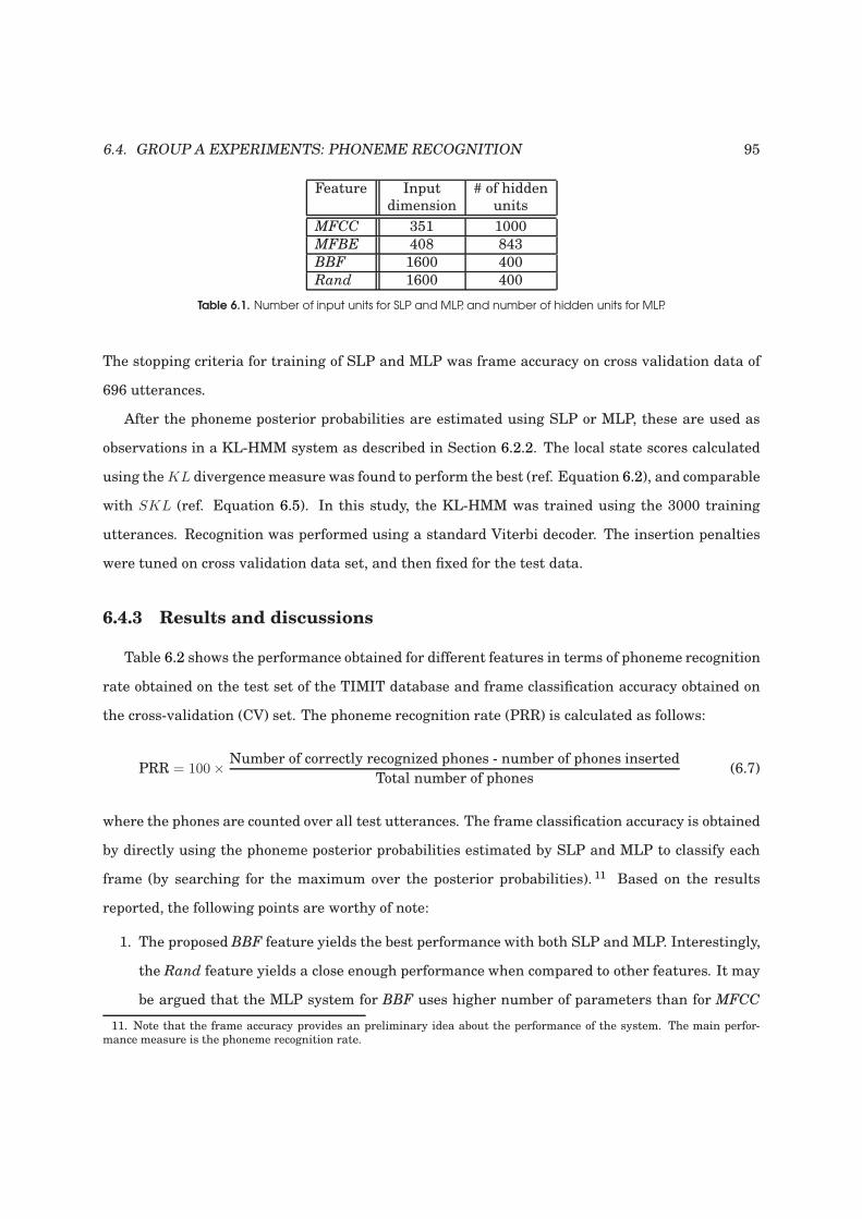
6.4. GROUP A EXPERIMENTS: PHONEME RECOGNITION 95
Feature Input # of hiddendimension units
MFCC 351 1000
MFBE 408 843
BBF 1600 400
Rand 1600 400
Table 6.1. Number of input units for SLP and MLP, and number of hidden units for MLP.
The stopping criteria for training of SLP and MLP was frame accuracy on cross validation data of
696 utterances.
After the phoneme posterior probabilities are estimated using SLP or MLP, these are used as
observations in a KL-HMM system as described in Section 6.2.2. The local state scores calculated
using theKL divergencemeasure was found to perform the best (ref. Equation 6.2), and comparable
with SKL (ref. Equation 6.5). In this study, the KL-HMM was trained using the 3000 training
utterances. Recognition was performed using a standard Viterbi decoder. The insertion penalties
were tuned on cross validation data set, and then fixed for the test data.
6.4.3 Results and discussions
Table 6.2 shows the performance obtained for different features in terms of phoneme recognition
rate obtained on the test set of the TIMIT database and frame classification accuracy obtained on
the cross-validation (CV) set. The phoneme recognition rate (PRR) is calculated as follows:
PRR = 100×Number of correctly recognized phones - number of phones inserted
Total number of phones(6.7)
where the phones are counted over all test utterances. The frame classification accuracy is obtained
by directly using the phoneme posterior probabilities estimated by SLP and MLP to classify each
frame (by searching for the maximum over the posterior probabilities). 11 Based on the results
reported, the following points are worthy of note:
1. The proposed BBF feature yields the best performance with both SLP and MLP. Interestingly,
the Rand feature yields a close enough performance when compared to other features. It may
be argued that the MLP system for BBF uses higher number of parameters than for MFCC
11. Note that the frame accuracy provides an preliminary idea about the performance of the system. The main perfor-mance measure is the phoneme recognition rate.

96 CHAPTER 6. APPLICATION TO AUTOMATIC SPEECH RECOGNITION
SLP MLPFeature CV Frame Phoneme CV Frame Phoneme
accuracy rec. rate (PRR) accuracy rec. rate (PRR)
MFCC 52.5 45.9 69.0 66.2
MFBE 52.4 46.6 68.2 66.6
BBF 64.4 62.8 69.1 67.8
Rand 59.5 56.2 67.3 65.0
Table 6.2. Frame accuracy on cross validation (CV) set and phoneme recognition rate on test set of the TIMIT databaseexpressed in %.
and MFBE and hence yields better performance. So, in order to verify it, we trained MLPs
for MFCC and MFBE features by increasing the number of hidden nodes to 1674 and 1462
respectively, to equalize the number of parameters. The performance for MFCC improved to
67.2% and for MFBE to 66.7%, which is still lower than the performance obtained with the
proposed feature.
It can be observed that the performance obtained with MFCC is lower than usually reported
performance (of around 68%) in the literature (Pinto et al., 2011; Ganapathy et al., 2009)
with hybrid HMM/MLP systems. This performance is achieved with speaker-level mean and
variance normalization of the cepstral features. In this work, for fair comparison between fea-
tures we did not perform speaker-level mean and variance normalization. However, the pro-
posed binary features approach the performance of other features such as Frequency Domain
Linear Prediction (FDLP) features (Ganapathy et al., 2009), M-RASTA features (Hermansky
and Fousek, 2005) and Perceptual Linear Prediction (PLP) features (Hermansky, 1990). The
reader may refer to (Ganapathy et al., 2009) for a comparison with all these features.
2. The study using SLP reveals interesting trends. The performance for BBF drops by 5% abso-
lute (about 7.4% relative), whereas forMFCC andMFBE, it drops drastically i.e., 20.3% (about
30.6% relative) and 20.0% (about 30% relative) respectively. There is a drop in performance
for Rand, however, it is about 10% absolute better than MFCC and MFBE.
3. The proposed BBF feature performs better than Rand thus showing the benefit of our
boosting-based approach. However, Rand achieves acceptable performance, especially if the
SLP performance is considered, where it performs significantly better thanMFCC andMFBE.
The extraction of both BBF and Rand in principle could be seen as a problem of finding a
sparse representation for phoneme recognition. In the area of pattern recognition and signal
6.5. GROUP B EXPERIMENTS: CONTINUOUS SPEECH RECOGNITION 97
processing, there are efforts towards finding such sparse representations. For example, in a
recent work on face recognition, it has been shown that the choice of feature is less crucial
if the sparsity of the recognition problem is harnessed properly (Wright et al., 2008). Our
studies may have implication towards this direction.
In summary, this preliminary work applied the proposed BBF-based approach to to the phoneme
recognition task on the TIMIT database and compared its performance with standard cepstral fea-
tures. Our studies showed that the proposed binary features can yield performance similar or better
than standard cepstral features.
6.5 Group B Experiments: Continuous Speech Recognition
The group of experiments reported in this section investigates: a) the scalability of these features
from the phoneme recognition task reported in Section 6.4 to the continuous speech recognition task
(i.e. word recognition), and b) the use of auxiliary data to select the features (Roy et al., 2011d).
The experiments in this group primarily use the DARPA Resource Management (RM) database.
6.5.1 Database description
The DARPA Resource Management (RM) corpus (Price et al., 1988) was used for the experi-
ments. The RM corpus consists of read queries on the status of naval resources. The database is
partitioned into training set (2,880 utterances), development set (1,110 utterances) and evaluation
set (1,200 utterances) (Dines and Magimai.-Doss, 2008). Training and development utterances are
spoken by 109 speakers and correspond to approximately 3.8 hours of speech data. Evaluation set
amounts to 1.1 hours of speech data and is covered by a word pair grammar included in the task
specification. The RM corpus has a vocabulary of 991 words. The phoneme-based lexicon was ob-
tained from the UNISYN dictionary. There are NΩ = 45 context-independent phonemes including
silence.
6.5.2 Systems evaluated and experimental details
Similar to the phoneme recognition studies in Section 6.4, several systems were evaluated. The
only difference in these systems was the type of features used. As before, we used a frame size of
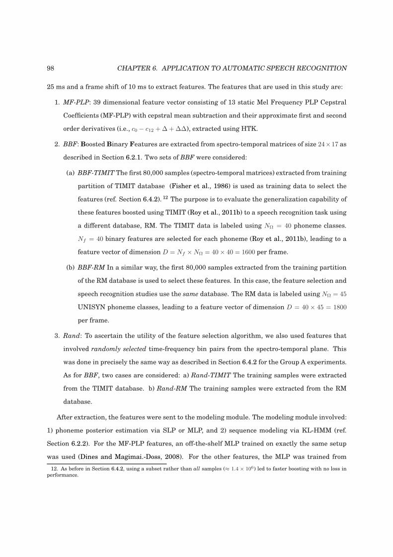
98 CHAPTER 6. APPLICATION TO AUTOMATIC SPEECH RECOGNITION
25 ms and a frame shift of 10 ms to extract features. The features that are used in this study are:
1. MF-PLP: 39 dimensional feature vector consisting of 13 static Mel Frequency PLP Cepstral
Coefficients (MF-PLP) with cepstral mean subtraction and their approximate first and second
order derivatives (i.e., c0 − c12 +∆+∆∆), extracted using HTK.
2. BBF: Boosted Binary Features are extracted from spectro-temporal matrices of size 24×17 as
described in Section 6.2.1. Two sets of BBF were considered:
(a) BBF-TIMIT The first 80,000 samples (spectro-temporalmatrices) extracted from training
partition of TIMIT database (Fisher et al., 1986) is used as training data to select the
features (ref. Section 6.4.2). 12 The purpose is to evaluate the generalization capability of
these features boosted using TIMIT (Roy et al., 2011b) to a speech recognition task using
a different database, RM. The TIMIT data is labeled using NΩ = 40 phoneme classes.
Nf = 40 binary features are selected for each phoneme (Roy et al., 2011b), leading to a
feature vector of dimension D = Nf ×NΩ = 40× 40 = 1600 per frame.
(b) BBF-RM In a similar way, the first 80,000 samples extracted from the training partition
of the RM database is used to select these features. In this case, the feature selection and
speech recognition studies use the same database. The RM data is labeled using NΩ = 45
UNISYN phoneme classes, leading to a feature vector of dimension D = 40 × 45 = 1800
per frame.
3. Rand: To ascertain the utility of the feature selection algorithm, we also used features that
involved randomly selected time-frequency bin pairs from the spectro-temporal plane. This
was done in precisely the same way as described in Section 6.4.2 for the Group A experiments.
As for BBF, two cases are considered: a) Rand-TIMIT The training samples were extracted
from the TIMIT database. b) Rand-RM The training samples were extracted from the RM
database.
After extraction, the features were sent to the modeling module. The modeling module involved:
1) phoneme posterior estimation via SLP or MLP, and 2) sequence modeling via KL-HMM (ref.
Section 6.2.2). For the MF-PLP features, an off-the-shelf MLP trained on exactly the same setup
was used (Dines and Magimai.-Doss, 2008). For the other features, the MLP was trained from
12. As before in Section 6.4.2, using a subset rather than all samples (≈ 1.4 × 10⁶) led to faster boosting with no loss inperformance.
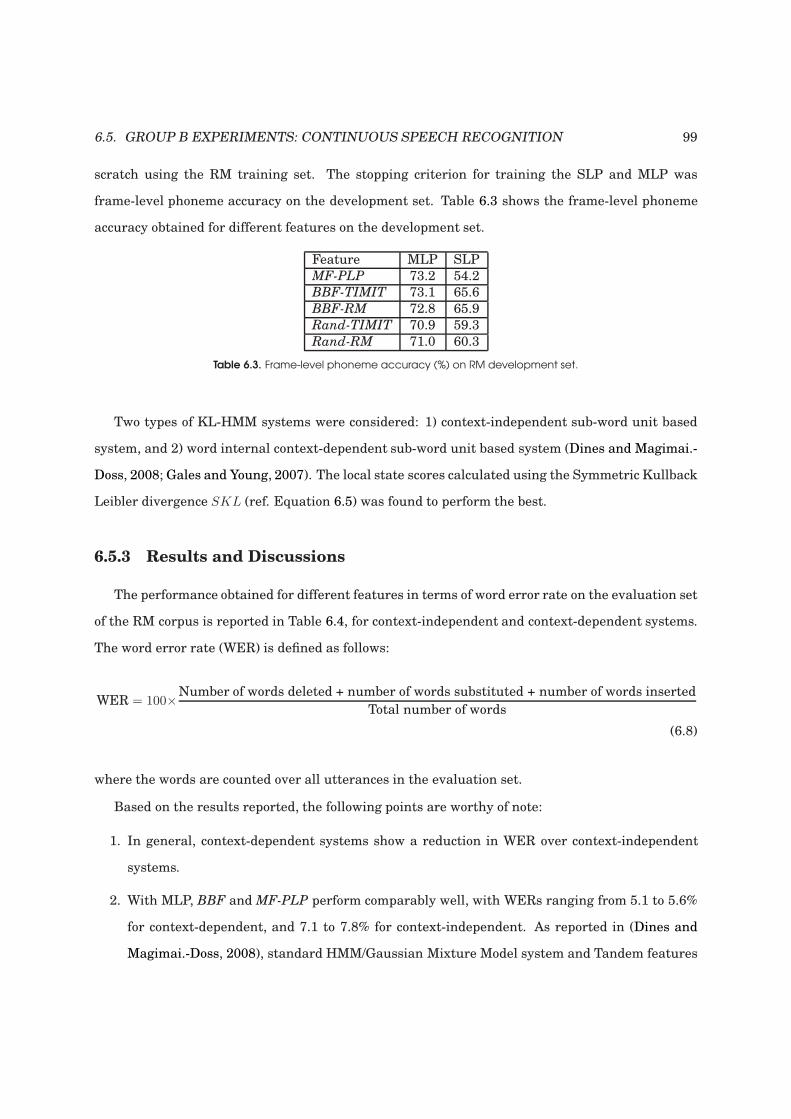
6.5. GROUP B EXPERIMENTS: CONTINUOUS SPEECH RECOGNITION 99
scratch using the RM training set. The stopping criterion for training the SLP and MLP was
frame-level phoneme accuracy on the development set. Table 6.3 shows the frame-level phoneme
accuracy obtained for different features on the development set.
Feature MLP SLP
MF-PLP 73.2 54.2
BBF-TIMIT 73.1 65.6
BBF-RM 72.8 65.9
Rand-TIMIT 70.9 59.3
Rand-RM 71.0 60.3
Table 6.3. Frame-level phoneme accuracy (%) on RM development set.
Two types of KL-HMM systems were considered: 1) context-independent sub-word unit based
system, and 2) word internal context-dependent sub-word unit based system (Dines and Magimai.-
Doss, 2008; Gales and Young, 2007). The local state scores calculated using the Symmetric Kullback
Leibler divergence SKL (ref. Equation 6.5) was found to perform the best.
6.5.3 Results and Discussions
The performance obtained for different features in terms of word error rate on the evaluation set
of the RM corpus is reported in Table 6.4, for context-independent and context-dependent systems.
The word error rate (WER) is defined as follows:
WER = 100×Number of words deleted + number of words substituted + number of words inserted
Total number of words
(6.8)
where the words are counted over all utterances in the evaluation set.
Based on the results reported, the following points are worthy of note:
1. In general, context-dependent systems show a reduction in WER over context-independent
systems.
2. With MLP, BBF and MF-PLP perform comparably well, with WERs ranging from 5.1 to 5.6%
for context-dependent, and 7.1 to 7.8% for context-independent. As reported in (Dines and
Magimai.-Doss, 2008), standard HMM/Gaussian Mixture Model system and Tandem features
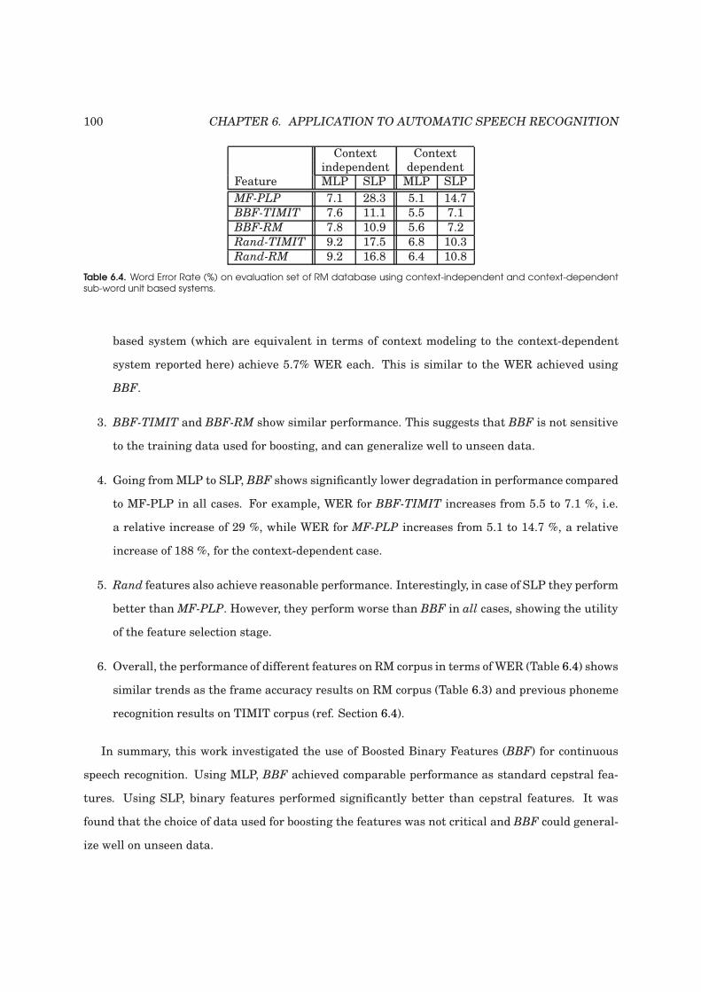
100 CHAPTER 6. APPLICATION TO AUTOMATIC SPEECH RECOGNITION
Context Contextindependent dependent
Feature MLP SLP MLP SLP
MF-PLP 7.1 28.3 5.1 14.7
BBF-TIMIT 7.6 11.1 5.5 7.1
BBF-RM 7.8 10.9 5.6 7.2
Rand-TIMIT 9.2 17.5 6.8 10.3
Rand-RM 9.2 16.8 6.4 10.8
Table 6.4. Word Error Rate (%) on evaluation set of RM database using context-independent and context-dependentsub-word unit based systems.
based system (which are equivalent in terms of context modeling to the context-dependent
system reported here) achieve 5.7% WER each. This is similar to the WER achieved using
BBF.
3. BBF-TIMIT and BBF-RM show similar performance. This suggests that BBF is not sensitive
to the training data used for boosting, and can generalize well to unseen data.
4. Going fromMLP to SLP, BBF shows significantly lower degradation in performance compared
to MF-PLP in all cases. For example, WER for BBF-TIMIT increases from 5.5 to 7.1 %, i.e.
a relative increase of 29 %, while WER for MF-PLP increases from 5.1 to 14.7 %, a relative
increase of 188 %, for the context-dependent case.
5. Rand features also achieve reasonable performance. Interestingly, in case of SLP they perform
better than MF-PLP. However, they perform worse than BBF in all cases, showing the utility
of the feature selection stage.
6. Overall, the performance of different features on RM corpus in terms ofWER (Table 6.4) shows
similar trends as the frame accuracy results on RM corpus (Table 6.3) and previous phoneme
recognition results on TIMIT corpus (ref. Section 6.4).
In summary, this work investigated the use of Boosted Binary Features (BBF) for continuous
speech recognition. Using MLP, BBF achieved comparable performance as standard cepstral fea-
tures. Using SLP, binary features performed significantly better than cepstral features. It was
found that the choice of data used for boosting the features was not critical and BBF could general-
ize well on unseen data.
6.6. GROUP C EXPERIMENTS: FUSION STUDIES 101
6.6 Group C Experiments: Fusion studies
It is evident that the standard cepstral features and the proposed BBF features are distinct in
nature: one is holistic and real-valued, while the other is localized and binary. This observation
suggests that they might carry useful complementary information. Hence, the objectives of this
section are: 1) to investigate the possible complementary nature of BBF and MFCC by analysing
their individual phoneme recognition performance on a subset of the TIMIT corpus at the frame
level, and 2) to implement a phoneme recognition system based on the fusion of BBF and MFCC
and evaluate it on the TIMIT corpus. In this context, two types of fusion strategies were studied:
a) feature fusion and b) decision fusion.
6.6.1 Analysis of complementary nature of BBF and cepstral features
We investigated the possible complementary nature of BBF and cepstral features using two
approaches. In the first approach, we analysed the distribution of frames from the cross validation
utterances of the TIMIT database according to whether they were correctly or incorrectly classified
by the MLPs trained using the two types of features. 13 More precisely, we divided the frames into
four groups:
1. Frames correctly classified by both MLPs (i.e. the MLP trained using BBF and the MLP
trained using cepstral features)
2. Frames correctly classified by the cepstral-based MLP but incorrectly classified by the BBF-
based MLP.
3. Frames incorrectly classified by the cepstral-based MLP but correctly classified by the BBF-
based MLP.
4. Frames incorrectly classified by both MLPs.
Table 6.5 shows the number of frames in each of the groups above. It is observed that 8.8% of the
frames were incorrectly classified using MFCC but correctly classified using BBF. Similarly, 9.2%
of the frames were incorrectly classified using BBF but correctly classified usingMFCC. This shows
that BBFmight be able to rectify some of the errors made byMFCC, and vice-versa. This indirectly
13. Note that these MLPs were trained using the training utterances from the TIMIT database as described in Sec-tions 6.2.2 and 6.4.2. In this case, the phoneme posterior estimates of the MLP are directly used to classify each frame intophonemes by searching for the phoneme with the maximum posterior estimate.
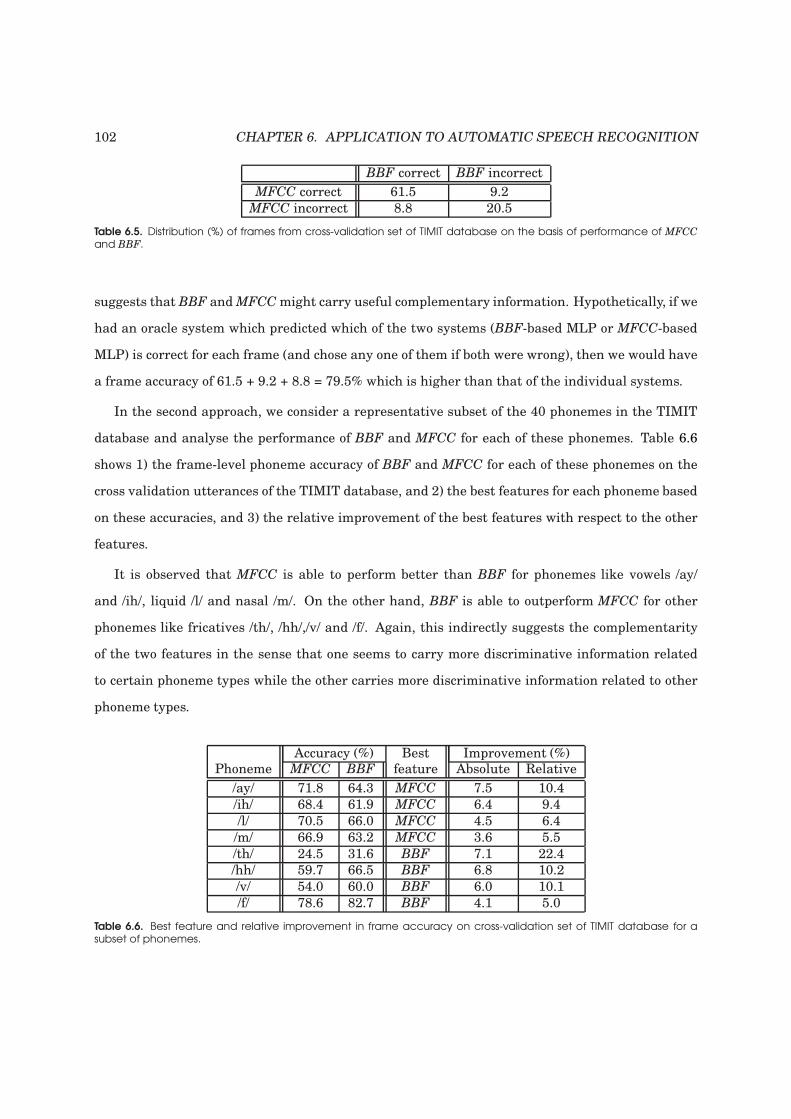
102 CHAPTER 6. APPLICATION TO AUTOMATIC SPEECH RECOGNITION
BBF correct BBF incorrect
MFCC correct 61.5 9.2
MFCC incorrect 8.8 20.5
Table 6.5. Distribution (%) of frames from cross-validation set of TIMIT database on the basis of performance of MFCC
and BBF.
suggests that BBF andMFCCmight carry useful complementary information. Hypothetically, if we
had an oracle system which predicted which of the two systems (BBF-based MLP or MFCC-based
MLP) is correct for each frame (and chose any one of them if both were wrong), then we would have
a frame accuracy of 61.5 + 9.2 + 8.8 = 79.5% which is higher than that of the individual systems.
In the second approach, we consider a representative subset of the 40 phonemes in the TIMIT
database and analyse the performance of BBF and MFCC for each of these phonemes. Table 6.6
shows 1) the frame-level phoneme accuracy of BBF and MFCC for each of these phonemes on the
cross validation utterances of the TIMIT database, and 2) the best features for each phoneme based
on these accuracies, and 3) the relative improvement of the best features with respect to the other
features.
It is observed that MFCC is able to perform better than BBF for phonemes like vowels /ay/
and /ih/, liquid /l/ and nasal /m/. On the other hand, BBF is able to outperform MFCC for other
phonemes like fricatives /th/, /hh/,/v/ and /f/. Again, this indirectly suggests the complementarity
of the two features in the sense that one seems to carry more discriminative information related
to certain phoneme types while the other carries more discriminative information related to other
phoneme types.
Accuracy (%) Best Improvement (%)Phoneme MFCC BBF feature Absolute Relative
/ay/ 71.8 64.3 MFCC 7.5 10.4
/ih/ 68.4 61.9 MFCC 6.4 9.4
/l/ 70.5 66.0 MFCC 4.5 6.4
/m/ 66.9 63.2 MFCC 3.6 5.5
/th/ 24.5 31.6 BBF 7.1 22.4
/hh/ 59.7 66.5 BBF 6.8 10.2
/v/ 54.0 60.0 BBF 6.0 10.1
/f/ 78.6 82.7 BBF 4.1 5.0
Table 6.6. Best feature and relative improvement in frame accuracy on cross-validation set of TIMIT database for asubset of phonemes.
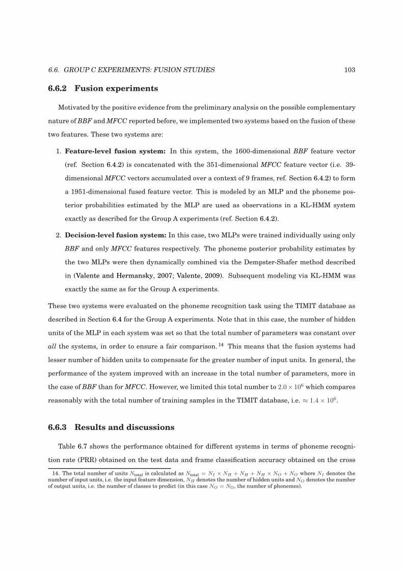
6.6. GROUP C EXPERIMENTS: FUSION STUDIES 103
6.6.2 Fusion experiments
Motivated by the positive evidence from the preliminary analysis on the possible complementary
nature of BBF andMFCC reported before, we implemented two systems based on the fusion of these
two features. These two systems are:
1. Feature-level fusion system: In this system, the 1600-dimensional BBF feature vector
(ref. Section 6.4.2) is concatenated with the 351-dimensional MFCC feature vector (i.e. 39-
dimensional MFCC vectors accumulated over a context of 9 frames, ref. Section 6.4.2) to form
a 1951-dimensional fused feature vector. This is modeled by an MLP and the phoneme pos-
terior probabilities estimated by the MLP are used as observations in a KL-HMM system
exactly as described for the Group A experiments (ref. Section 6.4.2).
2. Decision-level fusion system: In this case, two MLPs were trained individually using only
BBF and only MFCC features respectively. The phoneme posterior probability estimates by
the two MLPs were then dynamically combined via the Dempster-Shafer method described
in (Valente and Hermansky, 2007; Valente, 2009). Subsequent modeling via KL-HMM was
exactly the same as for the Group A experiments.
These two systems were evaluated on the phoneme recognition task using the TIMIT database as
described in Section 6.4 for the Group A experiments. Note that in this case, the number of hidden
units of the MLP in each system was set so that the total number of parameters was constant over
all the systems, in order to ensure a fair comparison. 14 This means that the fusion systems had
lesser number of hidden units to compensate for the greater number of input units. In general, the
performance of the system improved with an increase in the total number of parameters, more in
the case of BBF than for MFCC. However, we limited this total number to 2.0× 10⁶ which compares
reasonably with the total number of training samples in the TIMIT database, i.e. ≈ 1.4× 10⁶.
6.6.3 Results and discussions
Table 6.7 shows the performance obtained for different systems in terms of phoneme recogni-
tion rate (PRR) obtained on the test data and frame classification accuracy obtained on the cross
14. The total number of units Ntotal is calculated as Ntotal = NI × NH + NH + NH × NO + NO where NI denotes thenumber of input units, i.e. the input feature dimension,NH denotes the number of hidden units andNO denotes the numberof output units, i.e. the number of classes to predict (in this case NO = NΩ, the number of phonemes).
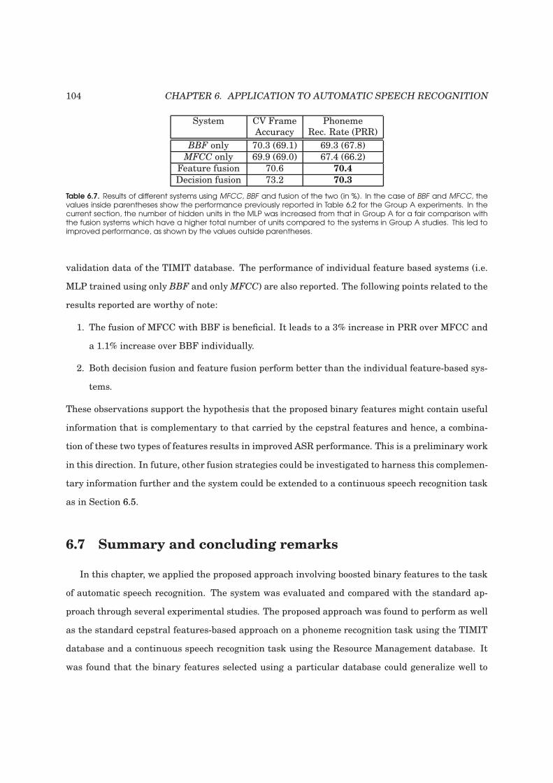
104 CHAPTER 6. APPLICATION TO AUTOMATIC SPEECH RECOGNITION
System CV Frame PhonemeAccuracy Rec. Rate (PRR)
BBF only 70.3 (69.1) 69.3 (67.8)
MFCC only 69.9 (69.0) 67.4 (66.2)
Feature fusion 70.6 70.4
Decision fusion 73.2 70.3
Table 6.7. Results of different systems using MFCC, BBF and fusion of the two (in %). In the case of BBF and MFCC, thevalues inside parentheses show the performance previously reported in Table 6.2 for the Group A experiments. In thecurrent section, the number of hidden units in the MLP was increased from that in Group A for a fair comparison withthe fusion systems which have a higher total number of units compared to the systems in Group A studies. This led toimproved performance, as shown by the values outside parentheses.
validation data of the TIMIT database. The performance of individual feature based systems (i.e.
MLP trained using only BBF and onlyMFCC) are also reported. The following points related to the
results reported are worthy of note:
1. The fusion of MFCC with BBF is beneficial. It leads to a 3% increase in PRR over MFCC and
a 1.1% increase over BBF individually.
2. Both decision fusion and feature fusion perform better than the individual feature-based sys-
tems.
These observations support the hypothesis that the proposed binary features might contain useful
information that is complementary to that carried by the cepstral features and hence, a combina-
tion of these two types of features results in improved ASR performance. This is a preliminary work
in this direction. In future, other fusion strategies could be investigated to harness this complemen-
tary information further and the system could be extended to a continuous speech recognition task
as in Section 6.5.
6.7 Summary and concluding remarks
In this chapter, we applied the proposed approach involving boosted binary features to the task
of automatic speech recognition. The system was evaluated and compared with the standard ap-
proach through several experimental studies. The proposed approach was found to perform as well
as the standard cepstral features-based approach on a phoneme recognition task using the TIMIT
database and a continuous speech recognition task using the Resource Management database. It
was found that the binary features selected using a particular database could generalize well to

6.7. SUMMARY AND CONCLUDING REMARKS 105
new data. Finally, the fusion of the proposed features with the standard cepstral features led to an
improvement in ASR performance at both the feature level and the decision level. This suggests
the possible complementary nature of the two types of features.

106 CHAPTER 6. APPLICATION TO AUTOMATIC SPEECH RECOGNITION
Chapter 7
Conclusions and future work
The standard approach to speaker and speech recognition involves cepstral features. These are
holistic, real-valued and based on prior knowledge of the human speech production and perception
systems. These features are typically modeled using Gaussian Mixture Models and Hidden Markov
Models.
In this thesis, we proposed a different approach for speaker and speech recognition based on
a novel set of features called Boosted Binary Features. These features are extracted by simple
comparison operations on time-frequency bin pairs of spectro-temporal segments of speech. The
features are binary-valued and selected in a data-driven way via the Adaboost algorithm.
The proposed approach is inspired by existing localized approaches in the computer vision do-
main such as boosted Haar features, Fern features and Local Binary Patterns. These approaches
have some important advantages: robustness and computational speed. These served as important
motivations for the proposed approach.
7.1 Application to speaker recognition
The proposed approach was applied to text-independent speaker recognition. For this purpose,
a very simple system was developed involving only comparisons and additions. The boosted binary
features were modeled by a linear weighted summation function. In order to evaluate the proposed
system, we carried out several experiments using a wide variety of databases and experimental
107

108 CHAPTER 7. CONCLUSIONS AND FUTURE WORK
conditions. The following databases were used:
1. TIMIT: This database was used to evaluate the performance of the system on clean speech
collected in near-ideal conditions in a noise-free environment.
2. Noisy TIMIT: This database was used to evaluate the performance of the system in the
presence of additive noise.
3. HTIMIT: The Handset TIMIT database was used to evaluate the performance of the system
in the presence of convolutive noise.
4. MOBIO: This database comprises of speech collected through mobile phones in a realistic
noisy scenario. It was used in the MOBIO Face and Speaker Verification Evaluation contest
at the ICPR 2010.
The following experimental conditions were investigated: 1) Matched condition In this case,
the speech used for training and testing were matched, in terms of environmental and channel
properties. 2) Mismatched condition In this case, the speech data used for training and testing
were mismatched. The mismatch could be manifested in different ways. For example, in the case of
the noisy TIMIT experiments, speech data used for training was clean while speech data for testing
was noisy. In the case of HTIMIT, speech data from a particular microphone type was used for
training, while data collected using all the 9 telephone headsets was used for testing. In the case of
MOBIO, the mismatch was at multiple levels, such as speech type mismatch and site mismatch.
The performance of the proposed approach was compared with that of the standard approach.
In the case of the standard approach, a baseline MFCC-GMM system as well as state-of-the-art
systems were used. The latter contained various additional modules such as feature normalization,
supervector SVMs and joint factor analysis over the basic MFCC-GMM framework.
The experimental results showed that the proposed approach performed reliably and compared
well with the standard approach on all databases and under all experimental conditions. In par-
ticular, it often showed more robustness in noisy mismatched scenarios compared to the standard
approach. At the same time, it performed as well as the standard approach in clean, matched sce-
narios. This echoes the robustness of existing localized approaches in speech and computer vision
domains.
7.2. APPLICATION TO SPEECH RECOGNITION 109
In addition, an analysis of the computational complexity of the proposed system and standard
system was carried out. The analysis revealed that the the proposed system was faster than the
standard system by a factor of approximately 102. This shows that the proposed system has signif-
icant advantage in terms of speed compared to the standard one.
Possible directions for future work in speaker recognition are listed below:
1. The fusion of the proposed approach with the standard cepstral features-based approach could
be interesting. Different fusion strategies like feature-level fusion, and decision fusion could
be studied. Due to the distinct nature of the two approaches, their fusion might capture
complementary information present in BBF and MFCC. This could lead to improved speaker
recognition performance.
2. The proposed approach could be evaluated on more databases, such as NIST speaker recog-
nition evaluation data. 1 Note that the MOBIO database already used in this work may be
considered as challenging as the NIST database.
7.2 Application to speech recognition
The proposed approach was applied to speech recognition. In this case, the features were se-
lected to distinguish one phoneme from all others instead of a client from other speakers. The
summation-based modeling module used for speaker recognition was not suitable for this task;
single layer perceptrons (SLP) and multilayer perceptrons (MLP) were used instead. The phoneme
posterior probabilities estimated by the SLP and MLP were provided as observations to a KL-HMM
system. For speech recognition, a Viterbi decoder was used.
Three groups of experiments were carried out as follows: Firstly, phoneme recognition exper-
iments were carried out using the TIMIT database. In this study, each utterance was decode in
terms of its constituent phonemes. The proposed BBF features were found to perform as well as
the standard cepstral features.
Secondly, continuous speech recognition experiments were carried out using the Resource Man-
agement database. Again, the proposed features fared reasonably and compared well with the
standard features.
1. Details about this group of databases can be found at http://www.itl.nist.gov/iad/mig/tests/sre/.
110 CHAPTER 7. CONCLUSIONS AND FUTURE WORK
Finally, the possible complementary nature of BBF and cepstral features was investigated by
performing fusion studies using the two systems. Feature level and decision level fusion was per-
formed. It was found that speech recognition performance improved for both cases, over individual
systems using only BBF or only cepstral features.
Possible directions for future work in ASR are outlined below:
1. The application of BBF to ASR was partly motivated by its good performance on the speaker
recognition task as reported in Chapter 5. In this task, BBF often showed better noise-
robustness than cepstral features. It would be interesting to verify if the noise-robust charac-
teristic of BBF carries over to the case of ASR also.
2. The proposed approach could be evaluated on more challenging databases involving larger
vocabularies, and more difficult scenarios like broadcast news.
3. The BBF are discrete-valued and has performed well with SLP. This indicates that they
may be suitably incorporated into simpler modeling frameworks like Conditional Random
Fields (Morris and Fossler-Lusier, 2008) with binary feature functions, instead of MLP fol-
lowed by KL-HMM as in this work. This could enable joint feature selection and sequence
modeling, i.e. a more integrated framework similar to the proposed system for speaker recog-
nition.
4. The extraction of binary features could be interpreted as adding another layer to the MLP
or SLP to learn phone-specific representations directly from the spectro-temporal plane using
auxiliary data. This could have the potential to complement deep-learning frameworks geared
towards similar objectives (Mohamed et al., 2011).
5. Further work related to fusion of the two approaches could be done to fully exploit the possible
complementary nature of BBF and cepstral features.
6. In this work, we used spectro-temporal representation derived from log mel filter bank ener-
gies. In principle, the extraction of BBF is not limited to the spectro-temporal representation.
For instance, it can be applied on phoneme posteriorgram (estimate of phoneme posterior
probabilities across time). Also, we restricted our studies to a context of 17 frames for fair
comparison with cepstral feature-based systems. The effect of using larger contexts for BBF
could be investigated. Furthermore, we used equal number of binary features i.e. 40, for

7.3. GENERAL DIRECTIONS FOR FUTURE WORK 111
all phonemes. This may not be necessary. The number of binary features could possibly be
decided for each phoneme in a data-driven manner.
7. In this work, a one-vs-all strategy was used to select the binary features. In this strategy, a
particular phoneme was set as the positive class and all the other phonemes were set as the
negative class, and features were selected for this combination. Features were then selected by
setting each phoneme as the positive class in turn and aggregated over all phonemes. While
this has worked well, other selection strategies could be promising as well. This includes
sharing features across classes (Torralba et al., 2006) and multiclass boosting strategies (Zhu
et al., 2009).
By following these directions, it is conjectured that BBF would be firmly established as an equal
alternative to cepstral features for ASR in the future.
7.3 General directions for future work
In addition to some of the directions relevant to the individual applications mentioned before,
the following are some general directions relevant to both tasks.
1. As BBF involves specific time-frequency points in the spectro-temporal matrix, it has the
potential to be directly coupled with suitable time-frequency masking frameworks for noise
removal (Lathoud et al., 2005) or signal separation (Yilmaz and Rickard, 2004).
2. The proposed features have an interesting property. They are selected in a data-driven and
task-specific way. Hence, analysis of the specific time-frequency bins corresponding to the
features selected by Adaboost could provide an insight on the related task (speaker or speech
recognition). This could reveal the precise information required for these tasks and which
time-frequency regions have more of this information. This could in turn be used to guide
further research in this direction.
3. The proposed approach is generic. Hence, it could be extended to applications in the audio
domain beyond speaker and speech recognition, for instance, music information retrieval (Ke
et al., 2005).

112 CHAPTER 7. CONCLUSIONS AND FUTURE WORK

Appendices
113

Appendix A
Localized Features for
Audio-Visual Person Recognition
Portable devices such as mobile phones have the potential to provide convenient access to such
services as e-banking and e-shopping provided it is protected by a reliable user authentication sys-
tem. Due to the availability of cameras and microphones in mobile devices, audio- and visual-based
biometrics can be used for this purpose. The goal of this work is to develop such a bimodal authen-
tication system fusing audio and visual modalities, satisfying the following criteria: 1) robustness
in uncontrolled real scenarios, for example in a noisy audio environment, and 2) suitable to be im-
plemented on a mobile phone, taking into account its relatively limited computational capabilities.
Multimodal fusion techniques involve either fusion at the feature level or at the score level
(Bengio, 2003; Ross et al., 2006; Sanderson, 2002). Feature-level fusion is rarely reported in the
literature, especially for audio-visual biometrics. This is mainly due to the curse of dimensional-
ity (Bishop, 1999) and its associated computational complexity. However, feature-level fusion has
an advantage: it does not assume statistical independence between the modalities as score fusion
often does. It has been shown that such an assumption is not always true (Roy and Marcel, 2010a)
and it could lead to a degradation in performance of score-level fusion systems (Nandakumar et al.,
2009). Thus it is important to investigate feature-level fusion systems too, at the same time trying
to overcome their inherent problem of dimensionality. In this work, we propose such a system based
115
116 APPENDIX A. LOCALIZED AUDIO-VISUAL FEATURES
on a novel concept of localized audio-visual features, coupled with a boosting framework for feature
selection (Friedman et al., 1998).
A.1 The Proposed Framework
A.1.1 Localized Audio-visual features: Slice classifiers
We assume that raw audio and visual streams have been synchronized and processed to give a
sequence of audio and visual feature vectors. Let us denote the audio and visual feature spaces by
Ra and Rv respectively. Let Na and Nv be the sizes of Ra and Rv respectively. The spaces Ra, Rv
can be combined to form the joint audio-visual feature space, Rav = Ra×Rv of size Nav = Na +Nv.
Let us define a slice L as a two-dimensional subspace of Rav. It is necessary that L has at least
one audio component La extracted from Ra and at least one visual component Lv extracted from
Rv. Since there are Na and Nv different audio and visual components in Ra and Rv respectively,
the total number of possible slices are NL = Na × Nv. Let Λ = LiNL
i=1 denote the complete set of
all possible slices. Each slice Li ∈ Λ is associated with a slice classifier hi, trained and tested on
projections of data exclusively on Li. Let H = hiNL
i=1 denote the complete set of slice classifiers.
We have selected the classifiers to be a quadratic discriminant functions (Duda et al., 2000). 1 For
a speaker authentication task, with client and impostor classes denoted by ‘1’ and ‘0’ respectively, a
slice classifier can be expressed as a function hi : Li → 0, 1. Given a point x ∈ Rav, let x(i) be its
projection on Li. Then,
hi(x(i)) =
1 if − (x(i) − µ1,i)TΣ−1
1,i (x(i) − µ1,i)+
(x(i) − µ0,i)TΣ−1
0,i (x(i) − µ0,i) ≥ θi
0 otherwise.
(A.1)
where µ1,i, µ0,i are the estimated means of classes ‘1’ and ‘0’ projected on Li, and Σ1,i, Σ0,i are their
estimated covariance matrices. The threshold θi is chosen to minimize misclassification error on the
training set. In this case, the slice classifier outputs (0 or 1) are the localized binary audio-visual
features.
1. Although other classifier types are possible, experiments have shown that it serves its purpose sufficiently well, without being toocomplex at the same time.
A.1. THE PROPOSED FRAMEWORK 117
Although a single slice classifier by itself is unlikely to perform sufficiently well in this task, it
is hypothesized that there will be at least some optimal slice classifiers which could be combined to
form a classifier strong enough for the task (Friedman et al., 1998).
A.1.2 Slice Classifier Selection and Combination by Boosting
Out of the complete set of slice classifiers H , a certain number of classifiers are iteratively se-
lected for each client according to their discriminative ability with respect to that client. This selec-
tion is based on the Discrete Adaboost algorithm (Friedman et al., 1998) with weighted sampling,
which is widely used for selection tasks and is known for its robust performance (Friedman et al.,
1998). The algorithm, which is to be run once for each client, is as follows: 2
Algorithm: Slice Classifier Selection by Discrete Adaboost
Inputs: Ntr training vectors xjNtr
j=1, corresponding class labels, yj ∈ 0, 1 (0:impostor, 1:client),
Nh, the number of classifiers to be selected, N∗tr, the number of training vectors to be randomly
sampled at each iteration (N∗tr < Ntr).
– Initialize the weights w1,j ←1
2N(0)tr
, 1
2N(1)tr
for yj = 0, 1 respectively, where N(0)tr and N
(1)tr are
the number of impostor and client training vectors respectively.
– Repeat for n = 1, 2, · · ·Nh:
– Normalize weights, wn,j ←wn,j
∑Ntrj′=1
wn,j′
– Randomly sample N∗tr training vectors, according to the distribution wn,j
– For each hi in H , choose θi to minimize misclassification error, ǫi =1
N∗tr
∑N∗tr
j=1 1hi(x(i)j
) 6=yj
over the sampled set.
– Select the next best classifier, h∗n = hi∗ where i∗ = argmini ǫi
– Set βn ←ǫi∗
1−ǫi∗
– Update the weights, wn+1,j ← wn,jβ1h∗
n(x(n)j
)=yj
n
Output: The sequence of selected best slice classifiers, h∗n
Nh
n=1.
For each client, the selected slice classifiers (i.e. the localized features) are combined linearly to
2. Note that this is essentially the same algorithm as used for boosting the binary features extracted from spectro-temporal segments of speech in Chapter 4.
118 APPENDIX A. LOCALIZED AUDIO-VISUAL FEATURES
give a strong classifier (Friedman et al., 1998), h(x) =∑Nh
n=1 αnhn(x(n)). The weights αn are
calculated to minimize the exponential loss (Friedman et al., 1998) and normalized to sum to unity
for each client, αn = log(βn)∑Nh
n′=1log(βn′ )
. Since a decision is only required at the utterance level and not
at the frame level, the responses h(x) of each frame x in an utterance are added and normalized by
the number of frames, to obtain the final score S for the utterance. This is compared with a preset
threshold to decide if the utterance was made by a client or an impostor. This preset threshold
Θ is calculated by minimizing the Equal Error Rate (EER) (Bimbot et al., 2004) on a separate
development set. The above framework is termed the Boosted Slice Classifier (BSC) framework.
A.2 Experiments
A.2.1 Database and Protocol
All experiments in this section were performed on the M2VTS database (M2VTS) using lip anno-
tations from http://www.ee.surrey.ac.uk/Projects/M2VTS/experiments/lip_tracking/.
We followed the speaker verification protocol for this database as outlined in (Bengio, 2003). This
protocol involves a 4-fold cross-validation procedure described as follows.
The clients were first divided into 4 disjoint sets, with 8 clients in each set. For each fold, one
particular set out of the four was set as the evaluation set, while the remaining 3 sets formed the
development set for that fold. The experiment was conducted in three phases: training, development
and evaluation, repeated individually for each fold.
In the training phase, the first and second recordings of each client were used to create client-
specific models. Negative samples for each client was obtained from the development set of that
fold. In the development phase, speaker verification is performed on the development set of each
fold using the third and fourth recordings of each client. The purpose is to select system parameters
(for e.g., the number of boosted classifiers Nh and the decision threshold Θ) that minimize EER on
this set (ref. Section A.1.2).
In the evaluation phase, speaker verification is performed on the evaluation set using the third
and fourth recordings of each client and using the optimal parameter values obtained from the
development phase of that fold. The verification performance (in terms of the mean HTER %) is
averaged over all 4 folds and reported. Since all system parameters were calculated using only
A.2. EXPERIMENTS 119
development data, this can be considered an unbiased estimate of the system performance in a real
scenario (Bengio, 2003).
Furthermore, for the evaluation phase, two different conditions were evaluated, a) Matched-
clean: The original clean data was used as it is. b) Mismatched-noisy: In this condition, two types
of noise, namely, white noise and babble noise, from the standard Noisex-92 database (Varga et al.,
1992) were added at 3 different SNR levels (10dB, 5dB and 0dB) to the original clean speech of
the third and fourth recording before testing. This represents a more difficult realistic scenario
where the evaluation data is noisy and hence mismatched with the training and development data
(Bengio, 2003). We report results for both these conditions.
A.2.2 Systems implemented
Two groups of speaker verification systems were implemented. The first group involves the
Boosted Slice Classifier (BSC) framework described in this work. The second group includes certain
reference systems which are conventionally used for audio-visual speaker verification with score-
level fusion. The performance of the two groups are compared.
The systems using the Boosted Slice Classifier framework (ref. Section A.1) were associated with
slices derived from an audio visual feature space pair. To form this pair, different audio and visual
feature spaces were investigated as described next. For each feature space, its code name (by which
it is indicated in subsequent sections) is provided in parentheses. For the audio feature space,
apart from the conventional cepstral representation of speech using 16 Mel Frequency Cepstral
Coefficients (MFCC) (Bimbot et al., 2004) (MC16), we also investigated magnitude spectra which
have shown promising performance in a similar boosting framework for speaker verification (Roy
et al., 2010). In particular, Mel spectra calculated using 24, 32 and 40 Mel filters (MS24, MS32 and
MS40) and Fourier spectra calculated using 256-point and 128-point Discrete Fourier Transform
(FS128, FS64) were investigated. For the visual feature space, a Region-of-Interest (ROI) around
the lips was extracted using available annotation. Next, either a 2D-DCT was performed on it and
the 15 highest energy coefficients were retained to form the features (DCT15) (Potamianos et al.,
2004) or the gray-scale values were directly used as features. Two ROI sizes were considered, a 16
× 16 ROI and an 8 × 8 ROI (GS256 and GS64 respectively).
Apart from the BSC systems, the following reference systems were implemented. For the audio
120 APPENDIX A. LOCALIZED AUDIO-VISUAL FEATURES
modality, a standard speaker verification system (Bimbot et al., 2004) using 16 MFCC, 16 ∆-MFCC
and∆-energy modelled by the UBM-GMM framework was implemented. We refer to this system as
MC-GMM. For the visual modality, a standard face verification system using block-based features
modelled by the UBM-GMM framework (Cardinaux et al., 2003; Lucey and Chen, 2004) was imple-
mented. From each block, 18 DCTmod2 features (Sanderson and Paliwal, 2002) were extracted. We
refer to this system as F-GMM. For audio-visual score fusion, the Normalization-based approach
(Jain et al., 2005; Sanderson and Paliwal, 2004; Poh and Kittler, 2009) was implemented. The fu-
sion score Sfusion is calculated as a simple sum of the scores from each modality, Sfusion =∑M
i=1 si
where siMi=1 denote the individual log-likelihood scores calculated from each modality. Here, the
number of modalities, M = 2.
A.2.3 Results
In Table A.1, we show the verification performance of the BSC framework, using different com-
binations of audio-visual space pairs. In Table A.1(a), we show the Matched-clean condition (ref.
Section A.2.1). In Tables A.1(b-g), we show 6 different cases for the Mismatched-noisy conditions
(2 noise types × 3 SNR levels). In Table A.2, we compare the performance of the reference systems
with some of the consistently better performing BSC systems.
A.3 Discussions
A.3.1 Speaker Verification Performance
Among the BSC systems, it is evident from Table A.1 that several out of the 18 audio-visual
feature space pairs investigated have performed well. Apart from reasonable performance in
the Matched-clean condition, they have shown significant robustness to the two types of noise at
medium to high noise levels in the Mismatched-noisy condition. This is a significant advantage
of the proposed framework. This noise robustness may be due to the fact that the noise might be
affecting some of the slices but not all the slices at the same time. Since the effect on one slice is
restricted only to that slice, the final output (linear sum of the slice classifier outputs) is affected
less than for a UBM-GMM based system in a similar noisy scenario.
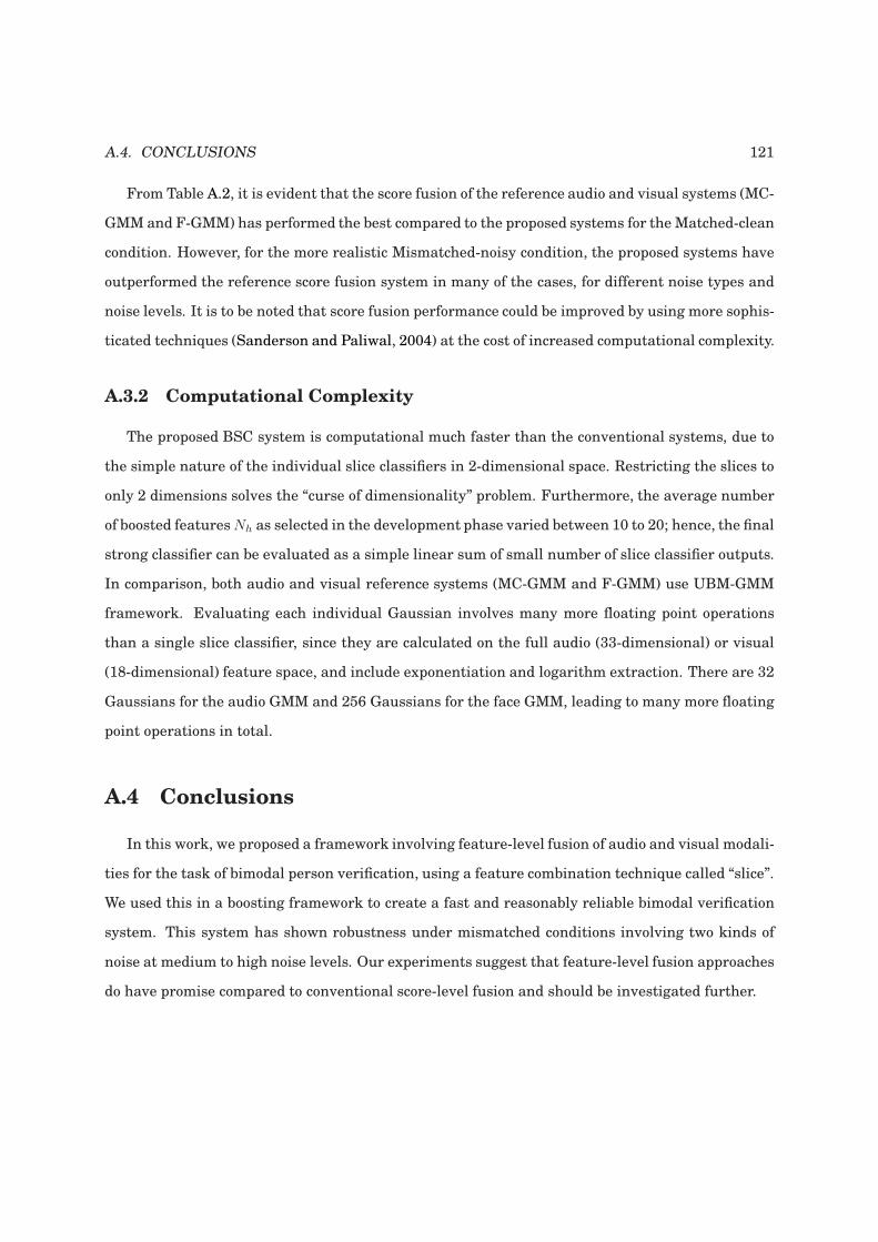
A.4. CONCLUSIONS 121
From Table A.2, it is evident that the score fusion of the reference audio and visual systems (MC-
GMMand F-GMM) has performed the best compared to the proposed systems for the Matched-clean
condition. However, for the more realistic Mismatched-noisy condition, the proposed systems have
outperformed the reference score fusion system in many of the cases, for different noise types and
noise levels. It is to be noted that score fusion performance could be improved by using more sophis-
ticated techniques (Sanderson and Paliwal, 2004) at the cost of increased computational complexity.
A.3.2 Computational Complexity
The proposed BSC system is computational much faster than the conventional systems, due to
the simple nature of the individual slice classifiers in 2-dimensional space. Restricting the slices to
only 2 dimensions solves the “curse of dimensionality” problem. Furthermore, the average number
of boosted featuresNh as selected in the development phase varied between 10 to 20; hence, the final
strong classifier can be evaluated as a simple linear sum of small number of slice classifier outputs.
In comparison, both audio and visual reference systems (MC-GMM and F-GMM) use UBM-GMM
framework. Evaluating each individual Gaussian involves many more floating point operations
than a single slice classifier, since they are calculated on the full audio (33-dimensional) or visual
(18-dimensional) feature space, and include exponentiation and logarithm extraction. There are 32
Gaussians for the audio GMM and 256 Gaussians for the face GMM, leading to many more floating
point operations in total.
A.4 Conclusions
In this work, we proposed a framework involving feature-level fusion of audio and visual modali-
ties for the task of bimodal person verification, using a feature combination technique called “slice”.
We used this in a boosting framework to create a fast and reasonably reliable bimodal verification
system. This system has shown robustness under mismatched conditions involving two kinds of
noise at medium to high noise levels. Our experiments suggest that feature-level fusion approaches
do have promise compared to conventional score-level fusion and should be investigated further.
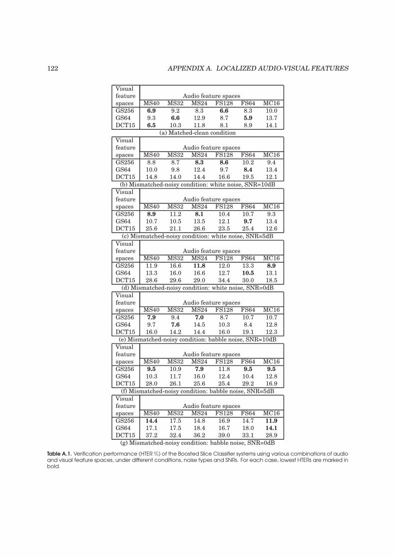
122 APPENDIX A. LOCALIZED AUDIO-VISUAL FEATURES
Visual
feature Audio feature spaces
spaces MS40 MS32 MS24 FS128 FS64 MC16
GS256 6.9 9.2 8.3 6.6 8.3 10.0
GS64 9.3 6.6 12.9 8.7 5.9 13.7
DCT15 6.5 10.3 11.8 8.1 8.9 14.1
(a) Matched-clean condition
Visual
feature Audio feature spaces
spaces MS40 MS32 MS24 FS128 FS64 MC16
GS256 8.8 8.7 8.3 8.6 10.2 9.4
GS64 10.0 9.8 12.4 9.7 8.4 13.4
DCT15 14.8 14.0 14.4 16.6 19.5 12.1
(b) Mismatched-noisy condition: white noise, SNR=10dB
Visual
feature Audio feature spaces
spaces MS40 MS32 MS24 FS128 FS64 MC16
GS256 8.9 11.2 8.1 10.4 10.7 9.3
GS64 10.7 10.5 13.5 12.1 9.7 13.4
DCT15 25.6 21.1 26.6 23.5 25.4 12.6
(c) Mismatched-noisy condition: white noise, SNR=5dB
Visual
feature Audio feature spaces
spaces MS40 MS32 MS24 FS128 FS64 MC16
GS256 11.9 16.6 11.8 12.0 13.3 8.9
GS64 13.3 16.0 16.6 12.7 10.5 13.1
DCT15 28.6 29.6 29.0 34.4 30.0 18.5
(d) Mismatched-noisy condition: white noise, SNR=0dB
Visual
feature Audio feature spaces
spaces MS40 MS32 MS24 FS128 FS64 MC16
GS256 7.9 9.4 7.0 8.7 10.7 10.7
GS64 9.7 7.6 14.5 10.3 8.4 12.8
DCT15 16.0 14.2 14.4 16.0 19.1 12.3
(e) Mismatched-noisy condition: babble noise, SNR=10dB
Visual
feature Audio feature spaces
spaces MS40 MS32 MS24 FS128 FS64 MC16
GS256 9.5 10.9 7.9 11.8 9.5 9.5
GS64 10.3 11.7 16.0 12.4 10.4 12.8
DCT15 28.0 26.1 25.6 25.4 29.2 16.9
(f) Mismatched-noisy condition: babble noise, SNR=5dB
Visual
feature Audio feature spaces
spaces MS40 MS32 MS24 FS128 FS64 MC16
GS256 14.4 17.5 14.8 16.9 14.7 11.9
GS64 17.1 17.5 18.4 16.7 18.0 14.1
DCT15 37.2 32.4 36.2 39.0 33.1 28.9
(g) Mismatched-noisy condition: babble noise, SNR=0dB
Table A.1. Verification performance (HTER%) of the Boosted Slice Classifier systems using various combinations of audioand visual feature spaces, under different conditions, noise types and SNRs. For each case, lowest HTERs are marked inbold.
A.4. CONCLUSIONS 123
Matched Mismatched-noisy
clean white noise babble noise
10dB 5dB 0dB 10dB 5dB 0dB
Reference MC-GMM (audio) 4.1 31.9 39.7 45.8 16.6 43.0 46.9
systems F-GMM (visual) 5.2 5.2 5.2 5.2 5.2 5.2 5.2
MC-GMM + F-GMM (score fusion) 2.8 8.3 15.2 28.1 2.6 10.2 25.0
BSC GS64-FS64 5.9 8.4 9.7 10.5 8.4 10.4 18.0
Systems GS256-MS24 8.3 8.3 8.2 11.8 7.0 7.9 14.8
Table A.2. Comparison of verification performance (HTER %) of the Boosted Slice Classifier (BSC) systems using theconsistently better performing combinations of audio and visual feature sets with the reference systems under variousconditions.

124 APPENDIX A. LOCALIZED AUDIO-VISUAL FEATURES
Appendix B
Haar Local Binary Patterns for
Fast Illumination Invariant Face
Detection
The main challenge for a face detection system is to successfully detect faces in an arbitrary
image, irrespective of variations in illumination conditions, background, pose, scale, expression and
the identity of the person. Numerous approaches have been proposed to counter these issues. Most
of these approaches can be organized in three categories: feature-based approaches (Heisele et al.,
2001), appearance-based approaches (Yang et al., 2000) and boosting-based approaches (Viola
and Jones, 2001). The third approach, which involves the boosting of simple local features called
Haar features in a cascade architecture, was introduced in 2001 by Viola and Jones (Viola and
Jones, 2001). It has become very popular since then because it shows very good results both in
terms of accuracy and speed (with the use of Integral Image concept), and is quite suitable for real-
time applications. Since the initial work of Viola and Jones, most of the research in face detection
has focused on the improvement of their cascade architecture. Related works can be classified in
mainly two possible directions: alternative boosting algorithms (Lyu, 2005), (Sun et al., 2004) or
alternative architecture designs (Luo, 2005), (Sochman and Matas, 2005).
However, most of these boosting-based methods which are derived from the Haar feature set
125

126 APPENDIX B. HLBP FEATURES FOR FACE DETECTION
have a common limitation. This is the vulnerability of the Haar feature set to variations in illumi-
nation conditions, for example, where there is a strong side illumination either from left or right,
or the dynamic range of the image intensity varies from region to region over the face (ref. Sec-
tion B.1.3). Thus, there is a need to improve the robustness of the system to take into account these
illumination variations, but retaining the richness of the feature set, and the advantages of efficient
feature selection by boosting and fast evaluation of the features using the Integral Image concept.
The Local Binary Pattern (LBP) introduced by Ojala et al. (Ojala et al., 1996) is one such operator
which is robust to monotonic illumination variations (ref. Figure B.1). Thus, various face detection
systems have been proposed using LBP or its variants, such as Improved Local Binary Patterns
(ILBP) (Jin et al., 2004), Multi-Block Local Binary Patterns (Zhang et al., 2007), the Modified
Census Transform (MCT) (Froba and Ernst, 2004), (Rodriguez, 2006) and the Locally Assembled
Binary (LAB) features (Yan et al., 2008).
In this work, we propose a new type of feature called the Haar Local Binary Pattern (HLBP)
feature which combines the advantages of both Haar and LBP. This feature compares the LBP label
counts in two adjacent image subregions, i.e. it indicates whether the number of times a particular
LBP label occurs in one region is greater or lesser than the number of times it occurs in another
region, offset by a certain threshold. These two subregions are represented by a set of masks similar
to Haar masks (Viola and Jones, 2001). Thus, our features are able to capture the region-specific
variation of local texture patterns. This makes our features more robust to illumination variations,
which may be quite complex and concentrated over certain subregions of the image only (strong
side illumination), compared to Haar and LBP individually. Since each LBP label count is actually
a particular bin value of the spatial histogram (Zhang et al., 2005), our features are also robust to
slight variations in location and pose.
To our knowledge, this is the first time individual LBP label counts have been combined with
Haar features for face detection. Since each HLBP feature is linked with exactly one LBP label,
there is no need to consider the entire LBP histogram in training and test, as in (Froba and Ernst,
2004). Thus our system is more efficient in terms of storage requirements as well as speed (ref. Sec-
tion B.2.2). This makes it more suitable for use on mobile devices for instance. We use a variation
of the Integral Histogram (Wang et al., 2006) to calculate our features, which further increases the
speed.
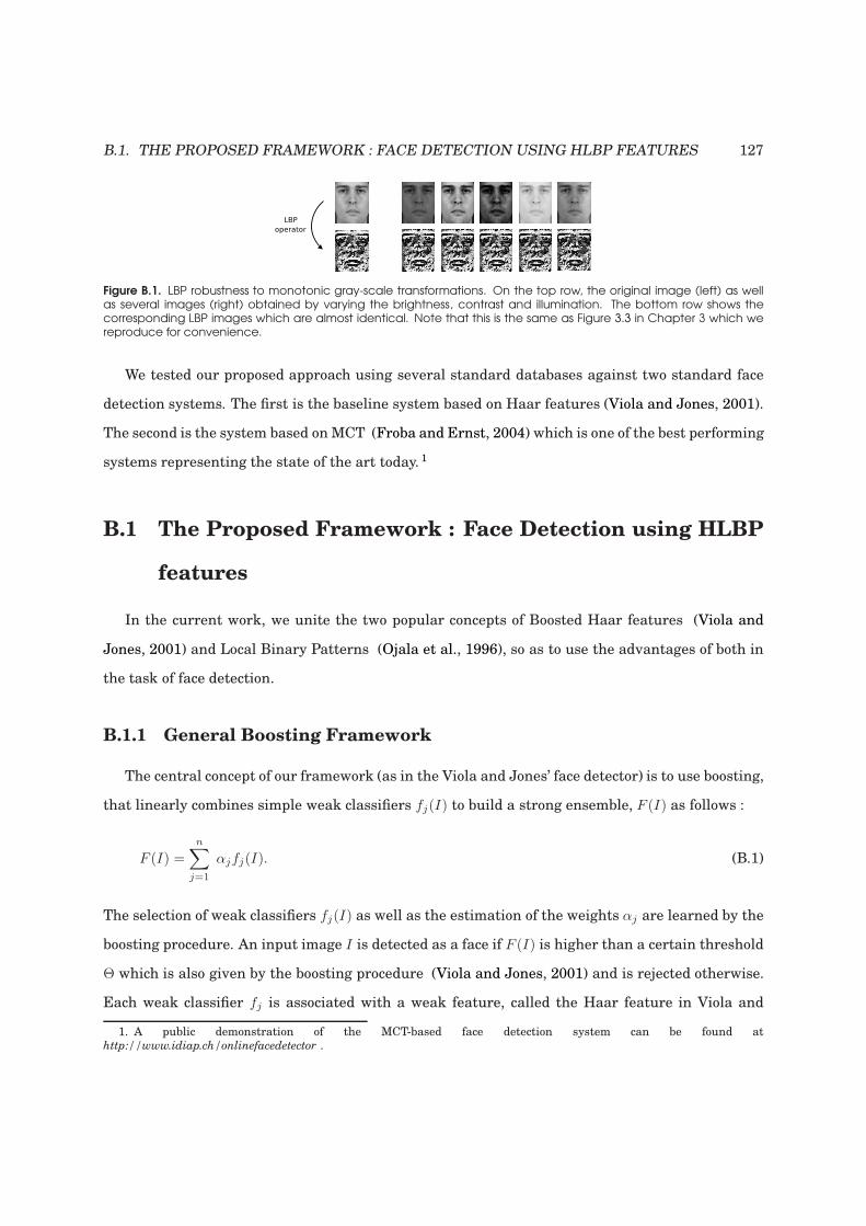
B.1. THE PROPOSED FRAMEWORK : FACE DETECTION USING HLBP FEATURES 127
Figure B.1. LBP robustness to monotonic gray-scale transformations. On the top row, the original image (left) as wellas several images (right) obtained by varying the brightness, contrast and illumination. The bottom row shows thecorresponding LBP images which are almost identical. Note that this is the same as Figure 3.3 in Chapter 3 which wereproduce for convenience.
We tested our proposed approach using several standard databases against two standard face
detection systems. The first is the baseline system based on Haar features (Viola and Jones, 2001).
The second is the system based onMCT (Froba and Ernst, 2004) which is one of the best performing
systems representing the state of the art today. 1
B.1 The Proposed Framework : Face Detection using HLBP
features
In the current work, we unite the two popular concepts of Boosted Haar features (Viola and
Jones, 2001) and Local Binary Patterns (Ojala et al., 1996), so as to use the advantages of both in
the task of face detection.
B.1.1 General Boosting Framework
The central concept of our framework (as in the Viola and Jones’ face detector) is to use boosting,
that linearly combines simple weak classifiers fj(I) to build a strong ensemble, F (I) as follows :
F (I) =n∑
j=1
αjfj(I). (B.1)
The selection of weak classifiers fj(I) as well as the estimation of the weights αj are learned by the
boosting procedure. An input image I is detected as a face if F (I) is higher than a certain threshold
Θ which is also given by the boosting procedure (Viola and Jones, 2001) and is rejected otherwise.
Each weak classifier fj is associated with a weak feature, called the Haar feature in Viola and
1. A public demonstration of the MCT-based face detection system can be found athttp://www.idiap.ch/onlinefacedetector .
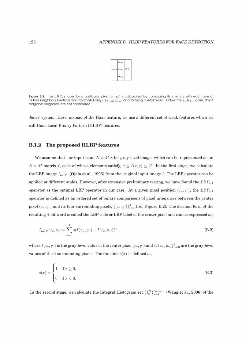
128 APPENDIX B. HLBP FEATURES FOR FACE DETECTION
Figure B.2. The LBP4,1 label for a particular pixel (xc, yc) is calculated by comparing its intensity with each one ofits four neighbors (vertical and horizontal only), xi, yi
3i=0
, and forming a 4-bit word. Unlike the LBP8,1 case, the 4diagonal neighbors are not considered.
Jones’ system. Here, instead of the Haar feature, we use a different set of weak features which we
call Haar Local Binary Pattern (HLBP) features.
B.1.2 The proposed HLBP features
We assume that our input is an N ×M 8-bit gray-level image, which can be represented as an
N ×M matrix I, each of whose elements satisfy, 0 ≤ I(x, y) ≤ 28. In the first stage, we calculate
the LBP image ILBP (Ojala et al., 1996) from the original input image I. The LBP operator can be
applied at different scales. However, after extensive preliminary testing, we have found the LBP4,1
operator as the optimal LBP operator in our case. At a given pixel position (xc, yc), the LBP4,1
operator is defined as an ordered set of binary comparisons of pixel intensities between the center
pixel (xc, yc) and its four surrounding pixels, (xi, yi)3i=0 (ref. Figure B.2). The decimal form of the
resulting 4-bit word is called the LBP code or LBP label of the center pixel and can be expressed as,
ILBP (xc, yc) =
3∑
n=0
s(I(xn, yn)− I(xc, yc))2n. (B.2)
where I(xc, yc) is the gray-level value of the center pixel (xc, yc) and I(xn, yn)3n=0 are the gray-level
values of the 4 surrounding pixels. The function s(x) is defined as,
s(x) =
1 if x ≥ 0,
0 if x < 0.
(B.3)
In the second stage, we calculate the Integral Histogram set IHk Nlabels
k=1 (Wang et al., 2006) of the
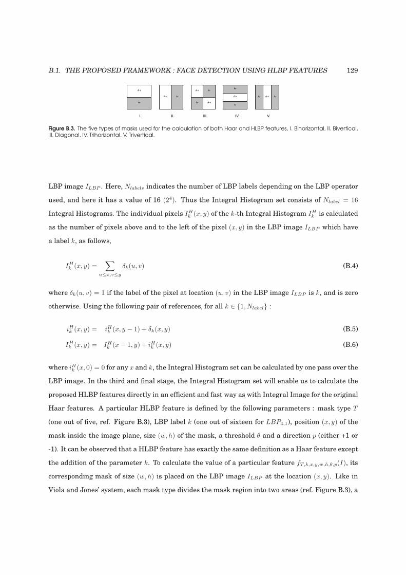
B.1. THE PROPOSED FRAMEWORK : FACE DETECTION USING HLBP FEATURES 129
Figure B.3. The five types of masks used for the calculation of both Haar and HLBP features, I. Bihorizontal, II. Bivertical,III. Diagonal, IV. Trihorizontal, V. Trivertical.
LBP image ILBP . Here, Nlabels indicates the number of LBP labels depending on the LBP operator
used, and here it has a value of 16 (24). Thus the Integral Histogram set consists of Nlabel = 16
Integral Histograms. The individual pixels IHk (x, y) of the k-th Integral Histogram IHk is calculated
as the number of pixels above and to the left of the pixel (x, y) in the LBP image ILBP which have
a label k, as follows,
IHk (x, y) =∑
u≤x,v≤y
δk(u, v) (B.4)
where δk(u, v) = 1 if the label of the pixel at location (u, v) in the LBP image ILBP is k, and is zero
otherwise. Using the following pair of references, for all k ∈ 1, Nlabel :
iHk (x, y) = iHk (x, y − 1) + δk(x, y) (B.5)
IHk (x, y) = IHk (x − 1, y) + iHk (x, y) (B.6)
where iHk (x, 0) = 0 for any x and k, the Integral Histogram set can be calculated by one pass over the
LBP image. In the third and final stage, the Integral Histogram set will enable us to calculate the
proposed HLBP features directly in an efficient and fast way as with Integral Image for the original
Haar features. A particular HLBP feature is defined by the following parameters : mask type T
(one out of five, ref. Figure B.3), LBP label k (one out of sixteen for LBP4,1), position (x, y) of the
mask inside the image plane, size (w, h) of the mask, a threshold θ and a direction p (either +1 or
-1). It can be observed that a HLBP feature has exactly the same definition as a Haar feature except
the addition of the parameter k. To calculate the value of a particular feature fT,k,x,y,w,h,θ,p(I), its
corresponding mask of size (w, h) is placed on the LBP image ILBP at the location (x, y). Like in
Viola and Jones’ system, each mask type divides the mask region into two areas (ref. Figure B.3), a
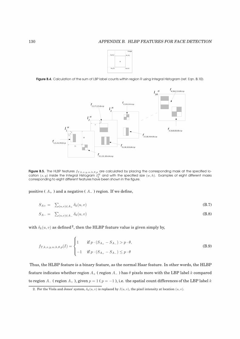
130 APPENDIX B. HLBP FEATURES FOR FACE DETECTION
Figure B.4. Calculation of the sum of LBP label counts within region R using Integral Histogram (ref. Eqn. B.10).
Figure B.5. The HLBP features fT,k,x,y,w,h,θ,p are calculated by placing the corresponding mask at the specified lo-
cation (x, y) inside the Integral Histogram IHk
and with the specified size (w, h). Examples of eight different maskscorresponding to eight different features have been shown in the figure.
positive ( A+ ) and a negative ( A− ) region. If we define,
SA+ =∑
(u,v)∈A+δk(u, v) (B.7)
SA− =∑
(u,v)∈A−δk(u, v) (B.8)
with δk(u, v) as defined2, then the HLBP feature value is given simply by,
fT,k,x,y,w,h,θ,p(I) =
1 if p · (SA+ − SA−) > p · θ,
−1 if p · (SA+ − SA−) ≤ p · θ
(B.9)
Thus, the HLBP feature is a binary feature, as the normal Haar feature. In other words, the HLBP
feature indicates whether region A+ ( region A− ) has θ pixels more with the LBP label k compared
to region A− ( region A+ ), given p = 1 ( p = −1 ), i.e. the spatial count differences of the LBP label k
2. For the Viola and Jones’ system, δk(u, v) is replaced by I(u, v), the pixel intensity at location (u, v).
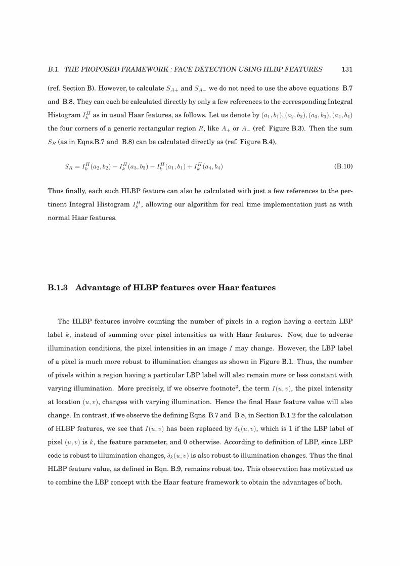
B.1. THE PROPOSED FRAMEWORK : FACE DETECTION USING HLBP FEATURES 131
(ref. Section B). However, to calculate SA+ and SA− we do not need to use the above equations B.7
and B.8. They can each be calculated directly by only a few references to the corresponding Integral
Histogram IHk as in usual Haar features, as follows. Let us denote by (a1, b1), (a2, b2), (a3, b3), (a4, b4)
the four corners of a generic rectangular region R, like A+ or A− (ref. Figure B.3). Then the sum
SR (as in Eqns.B.7 and B.8) can be calculated directly as (ref. Figure B.4),
SR = IHk (a2, b2)− IHk (a3, b3)− IHk (a1, b1) + IHk (a4, b4) (B.10)
Thus finally, each such HLBP feature can also be calculated with just a few references to the per-
tinent Integral Histogram IHk , allowing our algorithm for real time implementation just as with
normal Haar features.
B.1.3 Advantage of HLBP features over Haar features
The HLBP features involve counting the number of pixels in a region having a certain LBP
label k, instead of summing over pixel intensities as with Haar features. Now, due to adverse
illumination conditions, the pixel intensities in an image I may change. However, the LBP label
of a pixel is much more robust to illumination changes as shown in Figure B.1. Thus, the number
of pixels within a region having a particular LBP label will also remain more or less constant with
varying illumination. More precisely, if we observe footnote2, the term I(u, v), the pixel intensity
at location (u, v), changes with varying illumination. Hence the final Haar feature value will also
change. In contrast, if we observe the defining Eqns. B.7 and B.8, in Section B.1.2 for the calculation
of HLBP features, we see that I(u, v) has been replaced by δk(u, v), which is 1 if the LBP label of
pixel (u, v) is k, the feature parameter, and 0 otherwise. According to definition of LBP, since LBP
code is robust to illumination changes, δk(u, v) is also robust to illumination changes. Thus the final
HLBP feature value, as defined in Eqn. B.9, remains robust too. This observation has motivated us
to combine the LBP concept with the Haar feature framework to obtain the advantages of both.
132 APPENDIX B. HLBP FEATURES FOR FACE DETECTION
B.2 Experiments
We implemented a face detection system using our proposed HLBP features, and compared its
performance against two other reference face detection systems.
B.2.1 Reference systems and databases used
The first reference system is the one by Viola and Jones (Viola and Jones, 2001) using normal
Haar features. It provides the baseline for Haar feature-based systems. The second reference sys-
tem is the one by Froba et al. (Froba and Ernst, 2004; Rodriguez, 2006) using Modified Census
Transform (MCT). It is one of the LBP variants representing the current state of the art. To calcu-
late the MCT, Froba et al. compare each pixel in a 3 × 3 grid against the average of the intensity
values within that grid, instead of the center pixel as in LBP (ref. Section B.1.2). This leads to a 9-
bit code and a 511 (29−1)-bin Lookup table (LUT), each entry of which stores the log-likelihood ratio
of a particular code. This LUT has to be stored for each feature. The face detector is implemented
as a cascade of classifier stages, where each stage calculates the sum of LUT bins corresponding to
the MCT-codes at particular locations in the test image.
We implemented our system and both the reference systems as cascades of 5 stages. Each stage
had a strong classifier boosted from the set of weak classifiers (ref. Section B.1.1). The stages had
5, 10, 20, 50 and 200 weak classifiers respectively. Thus, the number of features is the same for all
the 3 systems.
For training, we used two internally created databases consisting of face and non-face images
extracted from BANCA(Spanish Corpus) (Bailly-Bailliere et al., 2003), Essex, Feret (Phillips et al.,
2000), ORL (Samaria and Young, 1994), Stirling and Yale (Belhumeur et al., 1997) databases. For
testing, we used 1) the standard XM2VTS database (Messer et al., 1999), (Luettin and Maitre,
2000), taking into account two cases, the Normal set with normal lighting conditions and the Dark-
ened set with adverse or side illumination, 3) the BioID database (Jesorsky et al., 2001) and 4)
an additional database from Fleuret et al. (Fleuret, 2004). A brief description of each database is
given in table B.1.
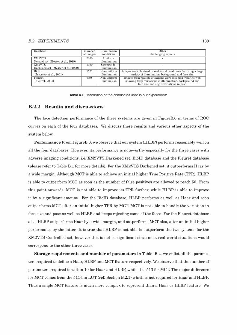
B.2. EXPERIMENTS 133
Database Number Illumination Otherof images conditions challenging aspects
XM2VTS 2360 Uniform -Normal set (Messer et al., 1999) illuminationXM2VTS 1180 Strong side- -Darkened set (Messer et al., 1999) illuminationBioID 1521 Non-uniform Images were obtained in real world conditions featuring a large(Jesorsky et al., 2001) illumination variety of illumination, background and face size.
Fleuret 580 Non-uniform Images from real life situations were collected from the web,(Fleuret, 2004) illumination showing large variations in illumination, background and
face size and slight variations in pose.
Table B.1. Description of the databases used in our experiments
B.2.2 Results and discussions
The face detection performance of the three systems are given in FigureB.6 in terms of ROC
curves on each of the four databases. We discuss these results and various other aspects of the
system below.
Performance From FigureB.6, we observe that our system (HLBP) performs reasonably well on
all the four databases. However, its performance is noteworthy especially for the three cases with
adverse imaging conditions, i.e, XM2VTS Darkened set, BioID database and the Fleuret database
(please refer to Table B.1 for more details). For the XM2VTS Darkened set, it outperforms Haar by
a wide margin. Although MCT is able to achieve an initial higher True Positive Rate (TPR), HLBP
is able to outperform MCT as soon as the number of false positives are allowed to reach 50. From
this point onwards, MCT is not able to improve its TPR further, while HLBP is able to improve
it by a significant amount. For the BioID database, HLBP performs as well as Haar and soon
outperforms MCT after an initial higher TPR by MCT. MCT is not able to handle the variation in
face size and pose as well as HLBP and keeps rejecting some of the faces. For the Fleuret database
also, HLBP outperforms Haar by a wide margin, and outperforms MCT also, after an initial higher
performance by the latter. It is true that HLBP is not able to outperform the two systems for the
XM2VTS Controlled set, however this is not so significant since most real world situations would
correspond to the other three cases.
Storage requirements and number of parameters In Table B.2, we enlist all the parame-
ters required to define a Haar, HLBP and MCT feature respectively. We observe that the number of
parameters required is within 10 for Haar and HLBP, while it is 513 for MCT. The major difference
for MCT comes from the 511-bin LUT (ref. Section B.2.1) which is not required for Haar and HLBP.
Thus a single MCT feature is much more complex to represent than a Haar or HLBP feature. We
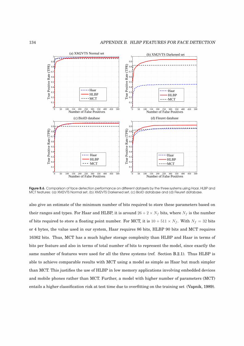
134 APPENDIX B. HLBP FEATURES FOR FACE DETECTION
0 50 100 150 200 250 300 350 400 450 5000
0.1
0.2
0.3
0.4
0.5
0.6
0.7
0.8
0.9
1
Number of False Positives
Tru
e P
ositi
ve R
ate
(TP
R)
(a) XM2VTS Normal set
HaarHLBPMCT
0 50 100 150 200 250 300 350 400 450 5000
0.1
0.2
0.3
0.4
0.5
0.6
0.7
0.8
0.9
1
Number of False Positives
Tru
e P
ositi
ve R
ate
(TP
R)
(b) XM2VTS Darkened set
HaarHLBPMCT
0 50 100 150 200 250 300 350 400 450 5000
0.1
0.2
0.3
0.4
0.5
0.6
0.7
0.8
0.9
1
Number of False Positives
Tru
e P
ositi
ve R
ate
(TP
R)
(c) BioID database
HaarHLBPMCT
0 50 100 150 200 250 300 350 400 450 5000
0.1
0.2
0.3
0.4
0.5
0.6
0.7
0.8
0.9
1
Number of False Positives
Tru
e P
ositi
ve R
ate
(TP
R)
(d) Fleuret database
HaarHLBPMCT
Figure B.6. Comparison of face detection performance on different datasets by the three systems using Haar, HLBP andMCT features: (a) XM2VTS Normal set, (b) XM2VTS Darkened set, (c) BioID database and (d) Fleuret database.
also give an estimate of the minimum number of bits required to store these parameters based on
their ranges and types. For Haar and HLBP, it is around 26 + 2×Nf bits, where Nf is the number
of bits required to store a floating point number. For MCT, it is 10 + 511 × Nf . With Nf = 32 bits
or 4 bytes, the value used in our system, Haar requires 86 bits, HLBP 90 bits and MCT requires
16362 bits. Thus, MCT has a much higher storage complexity than HLBP and Haar in terms of
bits per feature and also in terms of total number of bits to represent the model, since exactly the
same number of features were used for all the three systems (ref. Section B.2.1). Thus HLBP is
able to achieve comparable results with MCT using a model as simple as Haar but much simpler
than MCT. This justifies the use of HLBP in low memory applications involving embedded devices
and mobile phones rather than MCT. Further, a model with higher number of parameters (MCT)
entails a higher classification risk at test time due to overfitting on the training set (Vapnik, 1989).
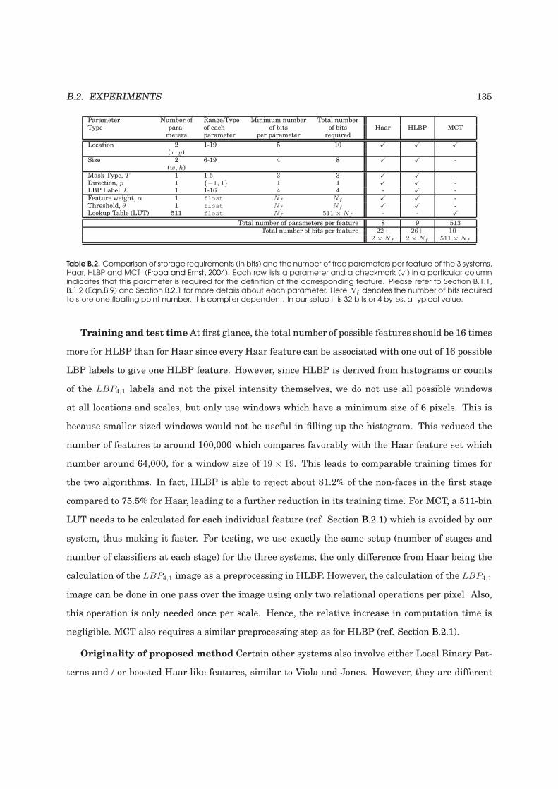
B.2. EXPERIMENTS 135
Parameter Number of Range/Type Minimum number Total numberType para- of each of bits of bits Haar HLBP MCT
meters parameter per parameter required
Location 2 1-19 5 10 X X X
(x, y)
Size 2 6-19 4 8 X X -(w, h)
Mask Type, T 1 1-5 3 3 X X -Direction, p 1 −1, 1 1 1 X X -LBP Label, k 1 1-16 4 4 - X -Feature weight, α 1 float Nf Nf X X -Threshold, θ 1 float Nf Nf X X -Lookup Table (LUT) 511 float Nf 511 × Nf - - X
Total number of parameters per feature 8 9 513Total number of bits per feature 22+ 26+ 10+
2 × Nf 2 × Nf 511 × Nf
Table B.2. Comparison of storage requirements (in bits) and the number of free parameters per feature of the 3 systems,Haar, HLBP and MCT (Froba and Ernst, 2004). Each row lists a parameter and a checkmark (X) in a particular columnindicates that this parameter is required for the definition of the corresponding feature. Please refer to Section B.1.1,B.1.2 (Eqn.B.9) and Section B.2.1 for more details about each parameter. Here Nf denotes the number of bits requiredto store one floating point number. It is compiler-dependent. In our setup it is 32 bits or 4 bytes, a typical value.
Training and test time At first glance, the total number of possible features should be 16 times
more for HLBP than for Haar since every Haar feature can be associated with one out of 16 possible
LBP labels to give one HLBP feature. However, since HLBP is derived from histograms or counts
of the LBP4,1 labels and not the pixel intensity themselves, we do not use all possible windows
at all locations and scales, but only use windows which have a minimum size of 6 pixels. This is
because smaller sized windows would not be useful in filling up the histogram. This reduced the
number of features to around 100,000 which compares favorably with the Haar feature set which
number around 64,000, for a window size of 19 × 19. This leads to comparable training times for
the two algorithms. In fact, HLBP is able to reject about 81.2% of the non-faces in the first stage
compared to 75.5% for Haar, leading to a further reduction in its training time. For MCT, a 511-bin
LUT needs to be calculated for each individual feature (ref. Section B.2.1) which is avoided by our
system, thus making it faster. For testing, we use exactly the same setup (number of stages and
number of classifiers at each stage) for the three systems, the only difference from Haar being the
calculation of the LBP4,1 image as a preprocessing in HLBP. However, the calculation of the LBP4,1
image can be done in one pass over the image using only two relational operations per pixel. Also,
this operation is only needed once per scale. Hence, the relative increase in computation time is
negligible. MCT also requires a similar preprocessing step as for HLBP (ref. Section B.2.1).
Originality of proposed method Certain other systems also involve either Local Binary Pat-
terns and / or boosted Haar-like features, similar to Viola and Jones. However, they are different
136 APPENDIX B. HLBP FEATURES FOR FACE DETECTION
from our proposed system. The Multi-Block Local Binary Pattern (Zhang et al., 2007) and Locally
Assembled Binary Feature (Yan et al., 2008) extend the idea of LBP by comparing sums of intensi-
ties over image patches to calculate the LBP label itself. The object detection framework by Zhang
et al. (Zhang et al., 2005) uses the concept of spatial histograms of Local Binary Patterns. Their
features measure the similarity between model and test histograms using histogram intersection
(Schiele, 1997). However, none of these methods compare counts of individual LBP labels in two
regions as we do. Our method tries to capture the region-specific variation of certain local texture
patterns, which is not done in (Zhang et al., 2007),(Yan et al., 2008) and (Zhang et al., 2005). Wang
et al. (Wang et al., 2006) have used Fisher Linear Discriminant on Histogram features for Face
Detection. However, there is no use of LBP concept which is the major contribution of our work.
Furthermore, the inclusion of Fisher Linear Discriminant increases the computational complexity
at test time.
B.3 Conclusions
In this work, we have introduced a new type of feature called the HLBP feature which combines
the concepts of Haar feature introduced by Viola and Jones, with Local Binary Patterns, harness-
ing the advantages of both for the problem of face detection. Our features are able to model the
region-specific variations of local texture and are relatively robust to wide variations in illumina-
tion, pose and background, and also slight variations in pose. Experiments have shown that our
system performs significantly better in such adverse imaging conditions than normal Haar fea-
tures and performs reasonably better than MCT features with much less storage and computation
requirements.

Bibliography
T. Ahonen, A. Hadid, and M. Pietikainen. Face recognition with local binary patterns. In Proceed-
ings 8th European Conference on Computer Vision (ECCV), pages 469–481, 2004.
J. Allen. How do Humans Process and Recognize Speech? IEEE Transactions on Speech and Audio
Processing, 2(4):567–577, 1994.
Y. Amit, A. Koloydenko, and P. Niyogi. Robust Acoustic Object Detection. Journal of the Acoustical
Society of America (JASA), 118(4):2634–2648, 2005.
G. Aradilla. Acoustic Models for Posterior Features in Speech Recognition. PhD thesis, Ecole Poly-
technique Federale de Lausanne, Lausanne, Switzerland, 2008.
G. Aradilla, H. Bourlard, and M. Magimai-Doss. Using KL-Based Acoustic Models in a Large Vo-
cabulary Recognition Task. In Proceedings of Interspeech, pages 928–931, 2008.
R. Auckenthaler, M. Carey, and H. Lloyd-Thomas. Score Normalization for Text-Independent
Speaker Verification System. Digital Signal Processing, 1(10):42–54, 2000.
E. Bailly-Bailliere, S. Bengio, F. Bimbot, M. Hamouz, J. Kittler, J. Mariethoz, J. Matas, K. Messer,
V. Popovici, F. Poree, B. Ruiz, and J.P. Thiran. The banca database and evaluation protocol.
In Proceedings of the 4th International Conference on Audio- and Video-Based Biometric Person
Authentication (AVBPA), pages 625–638, 2003.
P. Belhumeur, J. Hespanha, and D. Kriegman. Eigenfaces vs. Fisherfaces: Recognition Using Class
Specific Linear Projection. IEEE Transactions on Pattern Analysis and Machine Intelligence, 19
(7):711–720, 1997.
137
138 BIBLIOGRAPHY
S. Bengio. Multimodal Authentication using Asynchronous HMMs. In Proceedings of 4th Inter-
national Conference on Audio- and Video- based Biometric Person Authentication (AVBPA), vol-
ume 4. Springer, 2003.
Y. Bennani and P. Gallinari. Neural networks for discrimination and modelization of speakers.
Speech Communication, 17(1-2):159–175, August 1995.
L. Besacier, J.F. Bonastre, and C. Fredouille. Localization and selection of speaker-specific informa-
tion with statistical modeling. Speech Communication, 31(2-3):89–106, 2000.
F. Bimbot, J-F. Bonastre, C. Fredouille, G. Gravier, I. Magrin-Chagnolleau, S. Meignier, T. Merlin,
J. Ortega-Garcia, D. Petrovska-Delacretaz, and D.A. Reynolds. A Tutorial on Text-Independent
Speaker Verification. EURASIP Journal on Applied Signal Processing, 4:431–451, 2004.
C. Bishop. Neural Networks for Pattern Recognition. Oxford University Press, 1999.
H. Bourlard and S. Dupont. A new ASR approach based on independent processing and recombina-
tion of partial frequency bands. In Proceedings of International Conference on Spoken Language
Processing (ICSLP), pages 426–429, 1996.
H. Bourlard and N. Morgan. Connectionist Speech Recognition: A Hybrid Approach. Kluwer Aca-
demic Publishers, 1994.
H. Bourlard, S. Dupont, H. Hermansky, and N. Morgan. Towards sub-band-based speech recogni-
tion. In Proceedings of European Signal Processing Conference, pages 1579–1582, Trieste, Italy,
September 1996.
W. Campbell. Generalized linear discriminant sequence kernels for speaker recognition. In Pro-
ceedings of IEEE International Conference on Acoustics, Speech and Signal Processing (ICASSP),
volume 1, pages I–161–I–164, 2002.
W.M. Campbell, D.E. Sturim, and D.A. Reynolds. Support Vector Machines using GMM Supervec-
tors for Speaker Verification. IEEE Signal Processing Letters, 13(5):308–311, May 2006.
F. Cardinaux, C. Sanderson, and S. Marcel. Comparison of MLP and GMM classifiers for face
verification on XM2VTS. In Proceedings of International Conference on Audio- and Video- based
Biometric Person Authentication (AVBPA), pages 1058–1059, 2003.
BIBLIOGRAPHY 139
S.S. Chen and R. Gopinath. Gaussianization. In Proceedings of Neural Information Processing
Systems (NIPS), 2000.
T.H. Cormen, C.E. Leiserson, R.L. Rivest, and C. Stein. Introduction to Algorithms, chapter 1:
Foundations, pages 3–122. MIT Press and McGraw-Hill, 2001.
S.B. Davies and P. Mermelstein. Comparison of parametric representations for monosyllabic word
recognition in continously spoken sentences. IEEE Transactions on Acoustics, Speech and Signal
Processing, 28(4):357–366, 1980.
N. Dehak, R. Dehak, P. Kenny, N. Brummer, P. Ouellet, and P. Dumouchel. Support vector machines
versus fast scoring in the low-dimensional total variability space for speaker verification. In
Proceedings of Intespeech, pages 1559–1562, September 2009.
J. Dines and M. Magimai.-Doss. A study of phoneme and grapheme based context-dependent ASR
systems. In Proceedings of Machine Learning for Multimodal Interaction (MLMI) 2007, Lecture
Notes in Computer Science, 4892, pages 215–226, 2008.
R.O. Duda, P.E. Hart, and D.G. Stork. Pattern Classification. John Wiley and Sons, 2000.
W.M Fisher, G.R. Doddington, and K.M. Goudie-Marshall. The DARPA speech recognition research
database: Specifications and status. Proceedings of DARPA Workshop on Speech Recognition,
pages 93–99, February 1986.
H. Fletcher. Speech and Hearing in Communication. D. Van Nostrand Company, 1953.
F. Fleuret. Fast Binary Feature Selection with ConditionalMutual Information. Journal of Machine
Learning Research, 5:1531–1555, 2004.
J. Friedman, T. Hastie, and R. Tibshirani. Additive Logistic Regression: a Statistical View of Boost-
ing. Annals of Statistics, 28:2000, 1998.
B. Froba and A. Ernst. Face detection with the modified census transform. In Proceedings of Sixth
IEEE International Conference on Automatic Face and Gesture Recognition, pages 91–96, 2004.
S. Furui. Speaker-Independent IsolatedWord Recognition Using Dynamic Features of Speech Spec-
trum. IEEE Transactions on Acoustics, Speech and Signal Processing, 34(1):52–59, 1986.
140 BIBLIOGRAPHY
M. Gales and S. Young. The Application of Hidden Markov Models in Speech Recognition. Founda-
tions and Trends in Signal Processing, 1(3):195–304, 2007.
S. Ganapathy, S. Thomas, and H. Hermansky. Static and Dynamic Modulation Spectrum for Speech
Recognition. In Proceedings of Interspeech, pages 2823–2826, 2009.
J-L. Gauvain and C-H. Lee. Maximum A Posteriori Estimation for Multivariate Gaussian Mixture
Observations of Markov Chains. IEEE Transactions on Speech and Audio Processing, 2(2):291–
298, 1994.
T. Hain, P.C. Woodland, T.R. Niesler, and E.W.D.Whittaker. The 1998 HTK System for transcription
of conversational telephone speech. In Proceedings of IEEE International Conference on Audio,
Speech and Signal Processing (ICASSP), pages 57–60, 1999.
B. Heisele, T. Serre, M. Pontil, and T. Poggio. Component-based Face Detection. In Proceedings
of IEEE International Conference on Computer Vision and Pattern Recognition (CVPR), pages
657–662, 2001.
H. Hermansky. Perceptual linear predictive (PLP) analysis of speech. Journal of the Acoustical
Society of America, 87(4):1738–1752, 1990.
H. Hermansky and P. Fousek. Multi-Resolution RASTA Filtering for Tandem based ASR. Proceed-
ings of Interspeech, pages 361–364, 2005.
G. Heusch, Y. Rodriguez, and S. Marcel. Local Binary Patterns as an Im-
age Preprocessing for Face Authentication. In IEEE International Conference
on Automatic Face and Gesture Recognition (AFGR), pages 9–14, 2006. URL
ftp://ftp.idiap.ch/pub/papers/2006/heusch-AFGR-2006.pdf.
Intel 64 and IA-32 Architectures Optimization Reference Manual. Intel Corporation, August 2010.
A. Jain, K. Nandakumar, and A. Ross. Score Normalisation in Multimodal Biometric Systems.
Pattern Recognition, 38(12):2270–2285, 2005.
O. Jesorsky, K. Kirchberg, and R. Frischholz. Robust face detection using the hausdorff distance.
In Proceedings of the 3rd International Conference on Audio- and Video-Based Biometric Person
Authentication (AVBPA), pages 90–95, 2001.
BIBLIOGRAPHY 141
H. Jin, Q. Liu, H. Lu, and X. Tong. Face detection using improved lbp under bayesian framework. In
Proceedings of the Third International Conference on Image and Graphics (ICIG), pages 306–309,
2004.
Y. Ke, D. Hoiem, and R. Sukthankar. Computer Vision for Music Identification. In Proceedings of
the IEEE International Conference on Computer Vision and Pattern Recognition (CVPR), pages
597–604, 2005.
P. Kenny, G. Boulianne, P. Ouellet, and P. Dumouchel. Joint factor analysis versus eigenchannels
in speaker recognition. IEEE Transactions on Audio Speech and Language Processing, 15(4):
1435–1447, 2007.
M. Kleinschmidt and D. Gelbart. Improving Word Accuracy with Gabor Feature Extraction. In
Proceedings of International Conference of Spoken Language Processing (ICSLP), pages 25–28,
2002.
G. Lathoud, M. Magimai-Doss, B. Mesot, and H. Bourlard. Unsupervised Spectral Subtraction for
Noise-Robust ASR. In Proceedings of the IEEE Automatic Speech Recognition and Understanding
(ASRU) Workshop, pages 343 – 348, 2005.
K-F Lee and H-W Hon. Speaker-Independent Phone Recognition using Hidden Markov Models.
IEEE Transactions on Acoustics, Speech Signal Processing, 37(11):1641–1648, 1989.
S. Lucey and T. Chen. A GMM Parts Based Face Representation for Improved Ver-
ification through Relevance Adaptation. In Proceedings of IEEE International Confer-
ence on Computer Vision and Pattern Recognition (CVPR), pages 855–861, 2004. URL
http://amp.ece.cmu.edu/people/Simon/papers/slucey_cvpr04.pdf.
J. Luettin and G. Maitre. Evaluation protocol for the extended M2VTS database (XM2VTSDB).
Idiap Comm. 98-05, Idiap, 2000.
H.T. Luo. Optimization design of cascaded classifiers. In Proceedings of IEEE International Confer-
ence on Computer Vision and Pattern Recognition (CVPR), pages 480–485, 2005.
S.W. Lyu. Infomax Boosting. In Proceedings of IEEE International Conference on Computer Vision
and Pattern Recognition (CVPR), pages 533–538, 2005.
142 BIBLIOGRAPHY
M2VTS. M2VTS Multimodal Face Database, Release 1.00.
www.tele.ucl.ac.be/PROJECTS/M2VTS/m2fdb.html.
M. Magimai.-Doss, R. Rasipuram, G. Aradilla, and H. Bourlard. Grapheme-basedAutomatic Speech
Recognition Using KL-HMM. In Proceedings of Interspeech, 2011.
J. Makhoul. Linear prediction: A tutorial review. Proceedings of the IEEE, 63(5):561–580, April
1975.
S. Marcel, C. McCool, P. Matejka, T. Ahonen, and J. Cernocky. Mobile biometry (MOBIO) face and
speaker verification evaluation. Idiap Research Report Idiap-RR-09-2010, Idiap, May 2010a.
S. Marcel, C. McCool, P. Matejka, T. Ahonen, J. Cernocky, and S. Chakraborty. On the re-
sults of the first mobile biometry (MOBIO) face and speaker verification evaluation. In Pro-
ceedings of the 20th International Conference on Recognizing patterns in signals, speech, im-
ages, and videos, ICPR’10, pages 210–225, Berlin, Heidelberg, 2010b. Springer-Verlag. URL
http://portal.acm.org/citation.cfm?id=1939170.1939200.
D. Matrouf, N. Scheffer, B. Fauve, and J.-F. Bonastre. A straightforward and efficient implemen-
tation of the factor analysis model for speaker verification. In Proceedings of Interspeech, pages
1242–1245, 2007.
K. Messer, J. Matas, J. Kittler, J. Luttin, and G. Maitre. XM2VTSDB: The Extended M2VTS
Database. In Proceedings of the International Conference on Audio- and Video- based Biomet-
ric Person Authentication (AVBPA), pages 72–77, 1999.
A. Mohamed, G. Dahl, and G. E. Hinton. Acoustic modeling using deep belief network. IEEE
Transactions on Audio, Speech, and Language Processing (in press), 2011.
J. Morris and E. Fossler-Lusier. Conditional Random Fields for Integrating Local Discriminative
Classifiers. IEEE Transactions on Audio, Speech and Language Processing, 16(3):617–628, 2008.
K. Nandakumar, A. Ross, and A.K. Jain. Biometric fusion: Does modelling correlation really mat-
ter? In Proceedings of IEEE International Conference on Biometrics: Theory, Applications and
Systems (BTAS), pages 1–6, 2009.
BIBLIOGRAPHY 143
T. Ojala, M. Pietikainen, and D. Harwood. A comparative study of texture measures with classifi-
cation based on feature distributions. Pattern Recognition, 29(1):51–59, 1996.
M. Ozuysal, P. Fua, and V. Lepetit. Fast keypoint recognition in ten lines of code. In Proceedings of
IEEE International Conference on Computer Vision and Pattern Recognition (CVPR), pages 1–8,
2007.
J. Pelcanos and S. Sridharan. Feature warping for robust speaker verification. In Proceedings of
2001: A Speaker Odyssey Workshop, pages 213–218, June 2001.
P. Phillips, H. Moon, S. Rizvi, and P. Rauss. The feret evaluation methodology for face recognition
algorithms. IEEE Transactions on Pattern Analysis and Machine Intelligence (PAMI), 22(10):
1090–1104, 2000.
J. Pinto, G.S.V.S Sivaram, M. Magimai.-Doss, H. Hermansky, and H. Bourlard. Analysis of MLP
Based Hierarchical Phoneme Posterior Probability Estimator. IEEE Transcations on Audio,
Speech, and Language Processing, 19(2):225–241, 2011.
N. Poh and J. Kittler. Report on the description and evaluation of baseline algorithms for bimodal
authentication. Deliverable D4.2, MOBIO Mobile Biometry, 2009.
G. Potamianos, C. Neti, J. Luettin, and I. Matthews. Audio-visual automatic speech recognition: An
overview. In Issues in Visual and Audio-visual Speech Processing. MIT Press, 2004.
P. Price, W.M. Fisher, J. Bernstein, and D.S. Pallett. The DARPA 1000-word resource management
database for continuous speech recognition. In Proceedings of IEEE International Conference on
Acoustics, Speech and Signal Processing ICASSP, pages 651–654, 1988.
L.R. Rabiner. A tutorial on HiddenMarkov Models and selected applications in Speech Recognition.
In Proceedings of the IEEE, volume 77, pages 257–286, 1989.
D.A. Reynolds. A Gaussian Mixture modeling approach to text-independent speaker identification.
PhD thesis, Georgia Institute of Technology, September 1992.
D.A. Reynolds. Speaker identification and verification using Gaussian mixture speaker models.
Speech Communication, 17(1-2):91–108, 1995.
144 BIBLIOGRAPHY
D.A. Reynolds. HTIMIT and LLHDB: speech corpora for the study of handset transducer effects. In
Proceedings of IEEE International Conference on Audio, Speech and Signal Processing (ICASSP),
volume 2, pages 1535–1538, 1997.
D.A. Reynolds and R.C. Rose. Robust text-independent speaker identification using Gaussian mix-
ture speaker models. IEEE Transactions on Speech and Audio Processing, 3(1):72–83, 1995.
Y. Rodriguez. Face Detection and Verification using Local Binary Patterns. PhD Thesis 3681, Ecole
Polytechnique Federale de Lausanne, 2006.
A. Ross, K. Nandakumar, and A.K. Jain. Handbook of Multibiometrics. Springer Verlag, 2006.
A. Roy and S. Marcel. Haar Local Binary Pattern Feature for Fast Illumination Invariant Face
Detection. In Proceedings of British Machine Vision Conference, pages 1–12, September 2009.
A. Roy and S. Marcel. Crossmodal matching of speakers using lip and voice features in temporally
non-overlapping audio and video streams. In Proceedings of International Conference on Pattern
Recognition (ICPR), pages 4504–4507, 2010a.
A. Roy and S. Marcel. D4.4: Description and evaluation of advanced algorithms for joint bi-modal
authentication. Mobile biometry project deliverable, 2010b. URL www.mobioproject.org.
A. Roy, M. Magimai-Doss, and S. Marcel. Boosted binary features for noise-robust speaker verifica-
tion. In Proceedings of IEEE International Conference on Acoustics, Speech and Signal Processing
(ICASSP), pages 4442–4445, 2010.
A. Roy, M. Magimai.-Doss, and S. Marcel. A Fast Parts-based Approach to Speaker Verification
using Boosted Slice Classifiers. to appear in IEEE Transactions on Information Forensics and
Security, 2011a.
A. Roy, M. Magimai-Doss, and S. Marcel. Phoneme Recognition using Boosted Binary Features.
In Proceedings of IEEE International Conference on Acoustics, Speech and Signal Processing
ICASSP, pages 4868–4871, 2011b.
A. Roy, M. Magimai.-Doss, and S. Marcel. Fast Speaker Verification on Mobile Phone data using
Boosted Slice Classifiers. In Proceedings of IEEE IAPR International Joint Conference on Bio-
metrics (IJCB) (to appear), 2011c.
BIBLIOGRAPHY 145
A. Roy, M. Magimai.-Doss, and S. Marcel. Continuous speech recognition using boosted binary
features. Idiap Research Report Idiap-RR-35-2011, Idiap, October 2011d.
F. Samaria and S. Young. HMM-based Architecture for Face Identifica-
tion. Image and Vision Computing, 12(8):537–543, October 1994. URL
file:///home/vision/heusch/articles/Face/samariaICV94.pdf.
C. Sanderson. Automatic Person Verification Using Speech and Face Information. PhD thesis,
Griffith University, Queensland, Australia, 2002.
C. Sanderson and K. K. Paliwal. Fast feature extraction method for robust face verification. Elec-
tronic Letters, 38(25):1648–1650, 2002.
C. Sanderson and K.K. Paliwal. On the use of speech and face information for identity verification.
Research Report 04-10, Idiap Research Institute, 2004.
R.E. Schapire. The Strength of Weak Learnability. Machine Learning, 5(2):197–227, 1990.
B. Schiele. Object Recognition using Multidimensional Receptive Field Histograms. PhD thesis,
I.N.P.Grenoble, 1997.
K.T. Schutte. Parts-based Models and Local Features for Automatic Speech Recognition. Phd thesis,
Massachusetts Institute of Technology, 2009.
S. Sharma and H. Hermansky. Temporal patterns (TRAPS) in ASR of noisy speech. In Proceed-
ings of IEEE International Conference on Acoustics, Speech and Signal Processing (ICASSP),
volume 1, pages 289–292, 1999.
J. Sochman and J. Matas. WaldBoost-Learning for time constrained sequential detection. In Pro-
ceedings of IEEE International Conference on Computer Vision and Pattern Recognition (CVPR),
pages 150–156, 2005.
J.C. Steinberg. Positions of stimulation in the cochlea by pure tones. Journal of the Acoustical
Society of America, 8(3):176–180, 1937.
J. Sun, J.M. Rehg, and A.F. Bobick. Automatic cascade training with perturbation bias. In Pro-
ceedings of IEEE International Conference on Computer Vision and Pattern Recognition (CVPR),
pages 276–283, 2004.
146 BIBLIOGRAPHY
A. Torralba, K.P. Murphy, and W.T. Freeman. Shared Features for Multiclass Object Detection. In
Proceedings of Toward Category-Level Object Recognition, pages 345–361, 2006.
F. Valente. A Novel Criterion for Classifiers Combination in Multistream Speech Recognition. IEEE
Signal Processing Letters, 16(7):561–564, 2009.
F. Valente and H. Hermansky. Combination of Acoustic Classifiers based on Dempster-Shafer The-
ory of evidence. In Proceedings of IEEE International Conference on Acoustics, Speech, and Signal
Processing (ICASSP), volume 4, pages IV–1129 – IV–1132, 2007.
V.N. Vapnik. Statistical Learning Theory. Wiley-Interscience, 1989.
A.P. Varga, H.J.M Steeneken, M. Tomlinson, and D. Jones. The NOISEX-92 study on the effect of
additive noise on automatic speech recognition. Technical report, DRA Speech Research Unit,
1992.
P. Viola and M. Jones. Rapid object detection using a boosted cascade of simple features. In Proceed-
ings of the IEEE International Conference on Computer Vision and Pattern Recognition (CVPR),
pages 511–518, 2001.
A.J. Viterbi. Error bounds for convolutional codes and asymptotically optimum decoding algorithm.
IEEE Transactions on Information Theory, 13(2):260–269, 1967.
H. Wang, P. Li, and T. Zhang. Histogram features-based fisher linear discriminant for face detection.
In Proceedings of Asian Conference on Computer Vision (ACCV), pages 521–530, 2006.
J. Wright, A.Y. Yang, A. Ganesh, S.S. Sastry, and Y. Ma. Robust Face Recognition via Sparse
Representation. IEEE Transactions on Pattern Analysis and Machine Intelligence, 31(2):210–
227, March 2008.
S. Yan, S. Shan, X. Chen, and W. Gao. Locally Assembled Binary (LAB) Feature with Feature-
centric Cascade for Fast and Accurate Face Detection. In Proceedings of IEEE International
Conference on Computer Vision and Pattern Recognition (CVPR), pages 1–7, 2008.
M.-H. Yang, D. Roth, and N. Ahuja. A SNoW-based face detector. In Proceedings of Advances in
Neural Information Processing Systems (NIPS), pages 855–861, 2000.

BIBLIOGRAPHY 147
O. Yilmaz and S. Rickard. Blind Separation of Speech Mixtures by Time-Frequency Masking. IEEE
Transactions on Signal Processing, 52(7):1830–1847, July 2004.
K. K. Yiu, M. W. Mak, and S. W. Kung. Combining stochastic feature transformation and hand-
set identification for telephone-based speaker verification. In Proceedings of IEEE International
Conference on Acoustics, Speech and Signal Processing (ICASSP), volume 1, pages I–701 – I–704,
2002.
K. K. Yiu, M. W. Mak, and S. W. Kung. Environment adaptation for robust speaker verification by
cascading maximum likelihood linear regression and reinforced learning. Computer, Speech and
Language, 21(2):231–246, 2007.
H. Zhang, W. Gao, X. Chen, and D. Zhao. Learning informative features for spatial histogram-based
object detection. In Proceedings of International Joint Conference on Neural Networks (NIPS),
pages 1806–1811, 2005.
L. Zhang, R. Chu, S. Xiang, S. Liao, and S.Z. Li. Face detection based on Multi-Block LBP represen-
tation. In Proceedings of IEEE IAPR International Conference on Biometrics (ICB), pages 11–18,
2007.
J. Zhu, H. Zou, S. Rosset, and T. Hastie. Multi-class AdaBoost. Statistics and Its Interface, 2:
349–360, 2009.

148 BIBLIOGRAPHY

Curriculum Vitae
Name: Anindya Roy
Age: 28
Nationality: Indian
Permanent Address: 18/39 Ballygunge Place East, Kolkata 700029, India.
Email: [email protected]
General area of interest and expertise:
Pattern Recognition and signal processing in speech and computer vision domains.
Education:
1. August 2007 - October 2011
PhD in Electrical Engineering at the Ecole Polytechnique Federale de Lausanne, Switzerland
and the Idiap Research Institute, Martigny under the supervision of Prof. Herve Bourlard,
Dr. Sebastien Marcel and Dr. Mathew Magimai.-Doss (defense scheduled: 6th October 2011).
2. July 2005 - July 2007
Master of Technology in Electronics & Electrical Communication Engineering (Specializa-
tion: Automation & Computer Vision) at the Indian Institute of Technology, Kharagpur, India
(CGPA: 9.35 / 10).
3. July 2001 - July 2005
Bachelor of Engineering in Electronics and Telecommunication Engineering, Bengal Engi-
neering & Science University, Shibpur, India (1st class, 1st).
149
150 CURRICULUM VITAE
Professional Experience:
1. August 2007 - November 2011
Research Assistant at the Idiap Research Institute, Martigny, Switzerland.
2. July 2006 - June 2007
Teaching Assistant at the Indian Institute of Technology, Kharagpur, India.
Research Projects directly involved in:
1. MultiModal Interaction andMultiMedia Data Mining (MULTI), http://www.idiap.ch/scientific-
research/projects/multimodal-interaction-and-multimedia-data-mining
2. Interactive Multimodal Information Management (IM2), http://www.im2.ch/
3. MOBIO MObile BIOmetry (European FP7 project), www.mobioproject.org
Additional expertise:
1. Programming skills: MATLAB, C/C++, bash, Python, HTK, Quicknet, Qt for Nokia mobile
phone platform.
2. Contribution to the development of the machine vision library, Torch3Vision
(torch3vision.idiap.ch)
References:
1. Prof. Herve Bourlard, Idiap Research Institute, [email protected]
2. Dr. Sebastien Marcel, Idiap Research Institute, [email protected]
3. Dr. Mathew Magimai.-Doss, Idiap Research Institute, [email protected]
151
List of Publications:
Theses:
1. “Boosting Localized Features for Speaker and Speech Recognition”, PhD Thesis, Ecole Poly-
technique Federale de Lausanne, Lausanne, Switzerland, 2011.
2. “Multilevel KL Transform with Quantization Noise Feedback”, Masters Thesis, Indian Insti-
tute of Technology, Kharagpur, 2007.
Journal articles (peer-reviewed):
1. Anindya Roy, Mathew Magimai.-Doss and Sebastien Marcel, “A Fast Parts-based Approach
to Speaker Verification using Boosted Slice Classsifiers”, to appear in IEEE Transactions on
Information Forensics and Security, 2011.
Conference papers (peer-reviewed):
1. Anindya Roy, Mathew Magimai.-Doss and Sebastien Marcel, “Fast Speaker Verification on
Mobile Phone Data using Boosted Slice Classifiers”, in proceedings of the IEEE IAPR Inter-
national Joint Conference on Biometrics (IJCB) 2011.
2. Anindya Roy, Mathew Magimai.-Doss, and Sebastien Marcel, “Phoneme Recogni-
tion using Boosted Binary Features”, in proceedings of the IEEE International
Conference on Acoustics, Speech and Signal Processing (ICASSP), 2011. url:
http://publications.idiap.ch/index.php/publications/show/2030
3. Anindya Roy and Sebastien Marcel, “Introducing Crossmodal Biometrics: Person Identifi-
cation from Distinct Audio & Visual Streams”, in proceedings of the IEEE 4th Interna-
tional Conference on Biometrics: Theory, Applications and Systems (BTAS), 2010. url:
http://publications.idiap.ch/index.php/publications/show/1900
4. Anindya Roy and Sebastien Marcel, “Crossmodal Matching of Speakers using Lip and
Voice Features in Temporally Non-overlapping Audio and Video Streams”, in proceedings
of the 20th IAPR International Conference on Pattern Recognition (ICPR), 2010. url:
http://publications.idiap.ch/index.php/publications/show/1870
152 CURRICULUM VITAE
5. Anindya Roy, Mathew Magimai.-Doss, and Sebastien Marcel, “Boosted Binary Fea-
tures for Noise-Robust Speaker Verification”, in proceedings of the IEEE Interna-
tional Conference on Acoustics, Speech and Signal Processing (ICASSP), 2010. url:
http://publications.idiap.ch/index.php/publications/show/1808
6. Anindya Roy and Sebastien Marcel, “Visual processing-inspired Fern-Audio features for
Noise-Robust Speaker Verification”, in proceedings of the ACM 25th Symposium on Applied
Computing (SAC), 2010. url: http://publications.idiap.ch/index.php/publications/show/1746
7. Anindya Roy and Sebastien Marcel, “Haar Local Binary Pattern Feature for Fast Illumination
Invariant Face Detection”, in proceedings of the British Machine Vision Conference (BMVC),
2009. url: http://publications.idiap.ch/index.php/publications/show/1745
8. Sandipan Chakroborty, Anindya Roy and Gautam Saha, “Fusion of Complementary Feature
Set with MFCC for Improved Closed Set Text-Independent Speaker Identification” in proceed-
ings of the IEEE International Conference on Industrial Technology, Mumbai, 2006.
9. Sandipan Chakroborty, Anindya Roy, Sourav Majumdar and Gautam Saha, “Capturing Com-
plementary Information via Reversed Filter Bank and Parallel Implementation with MFCC
for Improved Text Independent Speaker Identification”, in proceedings of the International
Conference on Computing : Theory and Applications, Indian Statistical Institute Kolkata,
March 2007.
Technical Reports different from the above:
1. Anindya Roy, Mathew Magimai.-Doss and Sebastien Marcel, “Continuous Speech Recognition
using Boosted Binary Features”, Idiap Research Report Idiap-RR-35-2011, Idiap Research
Institute, October 2011
2. Anindya Roy and Sebastien Marcel, “Description and evaluation of advanced algo-
rithms for joint bi-modal authentication”, MOBIO project Deliverable D4.4. url:
http://www.mobioproject.org/Public/d4.4-description-and-evaluation-of-advanced/view