Embed Size (px)
Citation preview
325
Olivier J. BlanchardInternational Monetary Fund
Mark GriffithsInternational Monetary Fund
Bertrand GrussInternational Monetary Fund
Boom, Bust, Recovery: Forensics of the Latvia Crisis
ABSTRACT Latvia’s boom, bust, and recovery provide a rare case study for macroeconomists: an economy that responded to a balance-of-payments crisis by maintaining its currency peg and adjusting through internal devaluation and front-loaded consolidation. This paper lays down the facts about Latvia’s boom and bust and analyzes the policy response and the mechanics of the adjustment through internal devaluation. While Latvia’s adjustment was very costly, with a large drop in output, a big increase in unemployment, and substantial emigration, it was eventually successful. The internal devaluation worked faster, though quite differently, than what had been expected. Productivity increases, rather than nominal wage cuts, drove much of the unit labor cost reduction. These then led to an increase in profit margins, rather than a decrease in prices, and to a surprisingly fast supply response. The strong front-loaded adjustment did not prevent the recovery. The lessons of the Latvian experience for other countries may however be limited, since many of the elements of the eventual success appear to have been due to factors largely specific to Latvia, factors that are not present in southern euro countries, in particular.
latvia is a small country, with a population of only two million, yet it has been an object of intense attention during the financial crisis.
In response to their country’s own twin crises—in balance of payments and banking—and against the recommendations of many economists, the Latvian authorities decided to maintain their currency peg and adjust through internal devaluation and front-loaded fiscal austerity rather than devalue.
326 Brookings Papers on Economic Activity, fall 2013
Five years later, the proponents of this approach see it as a clear success. Its opponents see it, if not as a clear failure, at least as an excessively pain-ful adjustment. Witness the recent back-and-forth between Latvia’s prime minister, Valdis Dombrovskis, and Paul Krugman:
Krugman famously said back in December 2008 that Latvia is the new Argentina, it will inevitably go bankrupt, and now he has difficulty apparently admitting he was wrong and so he tries to seek some problems in how Latvia is recovering from the economic crisis [. . .] But I think that the mere fact that for the last two years we are enjoying rapid growth shows that it was probably the right strategy.
—Prime Minister Valdis Dombrovskis, March 15, 20131
The adulation over Latvia really tells us more about what the European policy elite wants to believe than it does either about the realities of Latvian experience or the fundamentals of macroeconomics. [. . .] We’re looking at a Depression-level slump, and five years later only a partial bounce back; unemployment is down but still very high, and the decline has a lot to do with emigration. It’s not what you’d call a triumphant success story.
—Paul Krugman, January 2, 20132
The main goal of this paper is to lay down the (often misstated) facts about Latvia’s adjustment. On its own, this would be a fascinating story of boom, bust, and (at least partial) recovery. But the story has wider relevance. Adjustment under a fixed exchange rate and the speed of fiscal consolidation have been and remain central issues in the euro debate, and Latvia is often used by one side or the other as an example of what to do or not to do. We hope our paper contributes toward moving this debate forward.
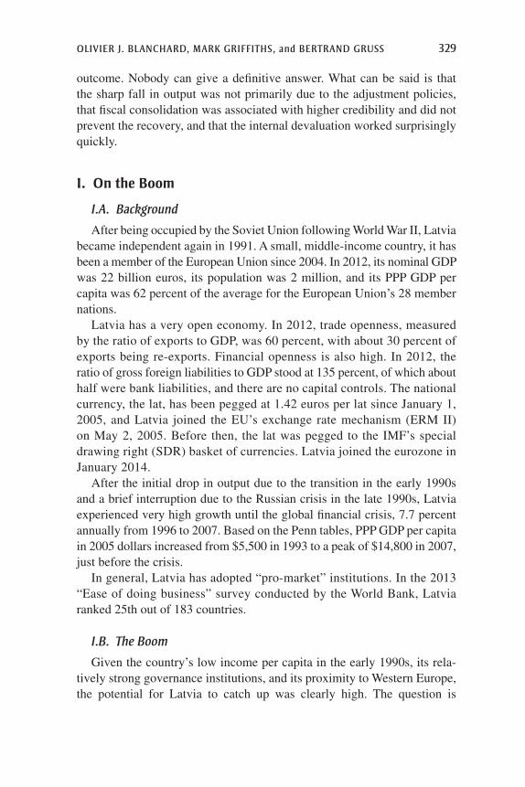
The basic and striking facts to be explained are illustrated in figure 1. GDP increased by almost 90 percent from 2000Q1 to 2007Q4, followed by a decrease of 25 percent from 2007Q4 to 2009Q3 and then a recovery, as of 2013Q2, of 18 percent. Meanwhile, the unemployment rate sketched a mirror image, decreasing from 14 percent in 2000Q1 to 6 percent in 2007Q4, then increasing to more than 21 percent by 2010Q1 and then decreasing since then to 11.4 percent as of 2013Q2.
We focus in this paper on six aspects of the story. These six key questions, and the answers we reached, may be summarized as follows.3
1. From Dombrovskis’ interview with CNBC at the EU summit in Brussels, quoted in “Krugman Can’t Admit He Was Wrong on Austerity: Latvia PM” and published on the CNBC.com website at http://www.cnbc.com/id/100558455.
2. From Krugman’s New York Times blog, “The Conscience of a Liberal,” dated January 2, 2013, and entitled “Latvia, Once Again.”
3. A lot has been written on Latvia. Two important references, which look at the various aspects of the boom and the bust, and from which we have benefited, are by Åslund and Dombrovskis (2011) and the set of articles in European Commission (2012).

Olivier J. Blanchard, Mark Griffiths, and Bertrand Gruss 327
First, What triggered the boom? The boom was triggered by a combina-tion of the country’s EU accession, belief in convergence to EU per capita incomes, cheap funds from foreign-owned banks, and optimistic expecta-tions. The boom was healthy at the start but, like many booms, increasingly bubbly and unbalanced at the end.
Second, What ended the boom? The end came in two stages. First, starting in 2007, a slowdown occurred due to rising inflation and loss of competitiveness, as well as tightening credit that reflected banks’ increasing worries about their loan books. Then, at the end of 2008, a collapse occurred due to the world financial crisis, leading to a sudden stop, a credit crunch, a sharp drop in exports, and increased uncertainty. Fiscal austerity came later, for the most part.
Third, What role did the sudden stop play in explaining the sharp decline in output? Liquidity provided by foreign banks, the central bank, and the Treasury reduced but did not eliminate the credit crunch. The decline in output was larger than what one would expect a credit crunch to trigger, however. Uncertainty after the sudden stop, together with the option value of waiting, were probably major additional factors.
Figure 1. real GdP and the unemployment rate (sa), latvia, 2000–13
10
15
20
25
80
120
160
2000 2002 2004 2006 2008 2010 2012
Unemployment (left-hand scale)
Real GDP (2000Q1=100, right-hand scale)
Source: Authors’ calculations.

328 Brookings Papers on Economic Activity, fall 2013
Fourth, What was the role of fiscal consolidation? Despite the public debate, it is hard to blame fiscal austerity for the decrease in output. Much of the fiscal adjustment was implemented after the main fall in output. There is suggestive evidence that commitment to a clear adjustment program—backed by substantial international financial support—increased confidence, as reflected in lower CDS spreads. However, much of the decrease in bor-rowing rates for households and firms was associated with the increased credibility of the peg and the decrease in exchange rate risk. This may have been partly the indirect result of fiscal consolidation through market per-ceptions that consolidation would ensure debt sustainability and also that it might make the disbursement of international support more likely.
Fifth, How did the internal devaluation work? It did work, but in ways different from the textbook adjustment. Public wages decreased sharply but with limited effects on private wages. Much of the improvement in unit labor costs, especially in the tradable sector, came from increases in pro-ductivity. This improvement in unit labor costs was only partly transmitted to prices, leading to an increase in firms’ profit margins. That was followed in turn by an increase in exports (but from the supply side more than the demand side, due to increased profitability), which was followed in turn by an increase in internal demand. On the supply side, part of the adjustment has happened through emigration, an adjustment not dissimilar to what happens across U.S. states.
Sixth, Has output returned to its full potential and unemployment returned to the natural rate? They have not yet returned, but they may not be very far from that point. There is no evidence that the natural unemployment rate is any higher now than it was before the crisis. But the evidence also shows that, given the market-friendly labor market institutions, the natural rate was surprisingly high before the crisis: probably around 10 percent or even higher. The difficulty is to pin down exactly what the natural rate was before the crisis.
Having laid out the facts, we return to the central issue. Is the Latvian adjustment a success story? In some ways, it clearly is a success. From a macroeconomic viewpoint, the Latvian economy is nearly back to where it was before the boom became unhealthy. While the unemployment rate is still somewhat higher than the (too high) natural rate, output is growing and the financial system is safer. Few other European countries can claim the same.
Nevertheless, the adjustment involved a very large decrease in output, a very large increase in unemployment, and substantial emigration. The question is whether an alternative strategy could have achieved a better
Olivier J. Blanchard, Mark Griffiths, and Bertrand Gruss 329
outcome. Nobody can give a definitive answer. What can be said is that the sharp fall in output was not primarily due to the adjustment policies, that fiscal consolidation was associated with higher credibility and did not prevent the recovery, and that the internal devaluation worked surprisingly quickly.
I. On the Boom
I.A. Background
After being occupied by the Soviet Union following World War II, Latvia became independent again in 1991. A small, middle-income country, it has been a member of the European Union since 2004. In 2012, its nominal GDP was 22 billion euros, its population was 2 million, and its PPP GDP per capita was 62 percent of the average for the European Union’s 28 member nations.
Latvia has a very open economy. In 2012, trade openness, measured by the ratio of exports to GDP, was 60 percent, with about 30 percent of exports being re-exports. Financial openness is also high. In 2012, the ratio of gross foreign liabilities to GDP stood at 135 percent, of which about half were bank liabilities, and there are no capital controls. The national currency, the lat, has been pegged at 1.42 euros per lat since January 1, 2005, and Latvia joined the EU’s exchange rate mechanism (ERM II) on May 2, 2005. Before then, the lat was pegged to the IMF’s special drawing right (SDR) basket of currencies. Latvia joined the eurozone in January 2014.
After the initial drop in output due to the transition in the early 1990s and a brief interruption due to the Russian crisis in the late 1990s, Latvia experienced very high growth until the global financial crisis, 7.7 percent annually from 1996 to 2007. Based on the Penn tables, PPP GDP per capita in 2005 dollars increased from $5,500 in 1993 to a peak of $14,800 in 2007, just before the crisis.
In general, Latvia has adopted “pro-market” institutions. In the 2013 “Ease of doing business” survey conducted by the World Bank, Latvia ranked 25th out of 183 countries.
I.B. The Boom
Given the country’s low income per capita in the early 1990s, its rela-tively strong governance institutions, and its proximity to Western Europe, the potential for Latvia to catch up was clearly high. The question is
330 Brookings Papers on Economic Activity, fall 2013
whether its high rate of growth before the crisis reflected healthy catch-up growth or something more.
Before looking at the specifics, it is useful to establish a benchmark. Using two variants of the Barro growth specification (Schadler and others 2006, and Vamvakidis 2008), which includes not only initial real income per capita, but also population growth, partner country growth, and a number of insti-tutional variables, we obtain the following. Until 2000, average growth of PPP GDP per capita was 6.2 percent, close to what these panel regressions predict. From 2001 to 2004, however, average growth was 8.2 percent, which is 1 to 3 percentage points higher than the regression predicts, and from 2005 to 2007 it was 11.6 percent, which is 4 to 6 percentage points higher than predicted.4 This suggests that starting in the 2000s, and especially from 2005 on, GDP growth in Latvia was higher than can be explained by catch-up. It also suggests that the boom became increasingly cyclical and, as will be seen, unhealthy.
With these results in mind, we start our story in 2000 and refer to the period 2000–07 as “the boom.” During that boom, average annual growth was 8.8 percent. The unemployment rate dropped from 14 percent in 2000 to 6 percent, its lowest level, at end-2007. Despite the peg, inflation rose to 10.1 percent in 2007 and to 15.3 percent in 2008, the highest in the European Union.
Viewed from the demand side, the boom came primarily from a rise in domestic demand. The ratio of private consumption to GDP (in constant prices) increased from 62 to 72 percent, and the ratio of investment to GDP (also in constant prices) from 22 to 36 percent.5 The growth in investment partly reflected a housing boom. Housing investment grew from 2 to 5 per-cent of GDP, with 40 percent of the increase in employment during the period taking place in construction (of which housing accounts for roughly one-third) and real estate. There were indeed good reasons for Latvian households and firms to increase their consumption and investment: the prospect of catch-up growth, the prospect of EU membership, and, later, the prospect of joining the eurozone, the last a goal that would be delayed by the crisis but has now (in January 2014) taken place.
As a matter of arithmetic, the result of increasing consumption and invest-ment ratios was a steady deterioration in the current account balance, with
4. See the online appendix to this paper for details of the two specifications, at http://www.brookings.edu/about/projects/bpea.
5. In current prices, the ratio of consumption to GDP remained nearly constant, while the ratio of investment to GDP increased from 23 percent to 40 percent, reflecting a large increase in the relative price of investment goods.
Olivier J. Blanchard, Mark Griffiths, and Bertrand Gruss 331
the ratio of the current account deficit to GDP increasing from 5 percent of GDP in 2000 to peak at a very large 25 percent in mid-2007.
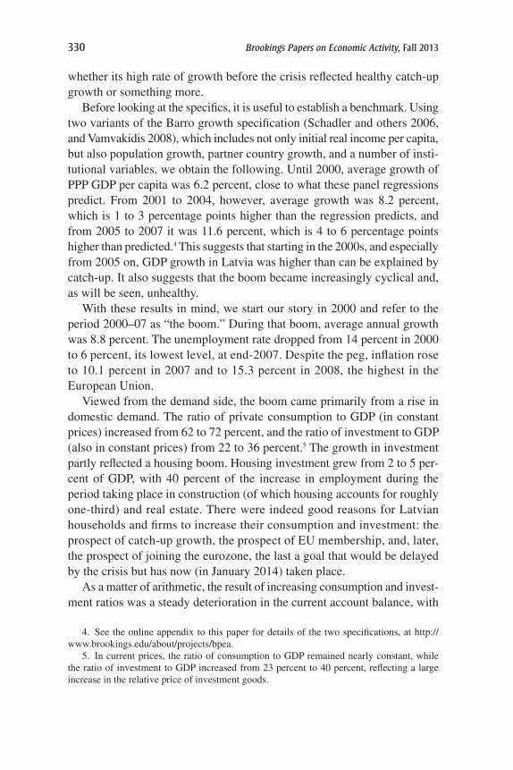
Once decomposed between exports and imports, the ratio of exports to GDP (in constant prices) remained roughly constant at 45 percent. This is impressive, given the high growth of the denominator—GDP growth—but might have been even higher were it not for supply constraints, as pro-duction shifted to the domestic market where demand was growing rapidly. On the other hand, the ratio of imports to GDP (also in constant prices) increased from 51 percent to 71 percent. If we think of imports as depending on domestic demand rather than on GDP, and given that domestic demand increased much faster than GDP, a more relevant statistic is the ratio of imports to domestic demand;6 this ratio went up from 49 percent to 58 per-cent. Thus, not only was domestic demand very strong, but it was accom-panied by a large shift toward foreign goods, leading to an even larger deterioration in the current account balance. (Figure 2 plots the evolution of exports, imports, and the trade balance.) Part of the shift probably reflected
6. We measure domestic demand here as private final consumption plus government final consumption plus gross capital formation.
2000 2002 2004 2006 2008 2010 2012
10
20
30
40
50
60
Trade deficit (left-hand scale)
Exports (right-hand scale)
Imports (right-hand scale)
Percent of GDPa Percent of GDP
Source: Authors’ calculations.a. National accounts basis, 4-quarter moving sum.
Figure 2. exports, imports, and the trade Balance, latvia, 2000–13
332 Brookings Papers on Economic Activity, fall 2013
the increasing real exchange rate appreciation (more on this below). Part of it may also have reflected a shift toward higher quality foreign products, an issue that will become relevant later when looking at the current account adjustment (see Bems and Di Giovanni 2013).
The current account deficit was easily financed, but with a worsening in the composition of financing over time. Foreign direct investment (FDI) increased from around 5 percent of GDP in 2000 to a peak of about 8 per-cent in mid-2007 before tailing off, perhaps an indication of worries about the persistence of the boom. However, even by 2007 the stock of FDI remained relatively low, 20 percent of GDP (and much of the FDI repre-sented capital increases of foreign bank branches and subsidiaries operat-ing in Latvia, which generated further credit expansion).
The rest of the financing was provided mainly by Swedish and other Nordic parent banks to their Latvian subsidiaries. Banks’ liabilities to foreign banks rose from 6 percent of GDP in 2000 to almost 54 percent in 2007.
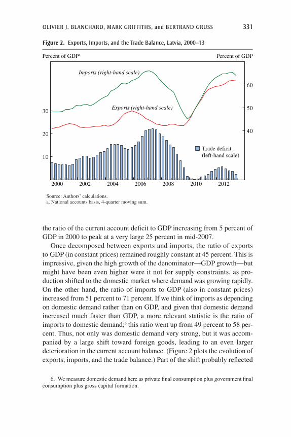
Throughout the boom, interest rates were low. Figure 3 plots a number of interest rates from 2004 onward. The 3-month money market rate decreased in the early 2000s, as Latvia repegged from the SDR to the euro, remaining around 4 percent until early 2007. Mortgage rates, which capture well the
Percent
5
10
15
20
2004 2006 2008 2010 2012
3-month money market
Mortgage rate, latsMortgage rate, euros
Source: Authors’ calculations.
Figure 3. latvia: nominal interest rates, 2004–13

Olivier J. Blanchard, Mark Griffiths, and Bertrand Gruss 333
evolution of private borrowing rates in general, in Latvia remained below 6 percent (in euros) until 2007. Mortgage rates in lats increased from 2007 on, reaching about 14 percent by the end of 2007, with the premium reflect-ing a growing perceived risk in the exchange rate. But, given the increas-ing inflation, even real mortgage rates issued in lats (constructing the real rate as the nominal rate minus current CPI inflation) were roughly equal to zero from 2004 onward, and real mortgage rates in euros were increasingly negative. Using wage or house price inflation, one finds that real interest rates were even more negative.
Associated with foreign financing through banks was very high credit growth, which grew by end-2007 to almost 10 times its 2001 level, an annual average growth rate of 33 percent in real terms. While the ratio of private sector credit to GDP was less than 20 percent in 2000, it reached almost 90 percent in 2007, higher than in other emerging European economies, although still lower than the euro area average. The proportion of loans denominated in foreign currency (initially mostly in dollars, but by the end almost entirely in euros) also increased steadily, rising from 50 percent in 2001 to more than 85 percent in 2007.7
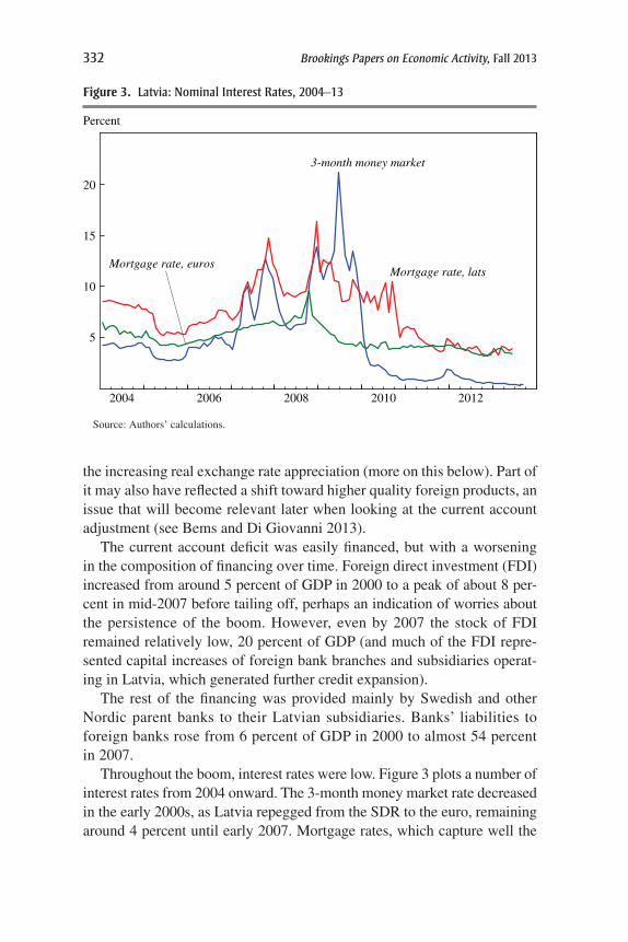
There were few signs of overheating until 2005, consistent with the notion that high growth until then reflected mostly potential growth. Starting in 2006, however, signs of overheating became much clearer. Wages and prices increased rapidly. As shown in figure 4, unit labor costs (ULCs), normalized to 100 in 2000, reached 135 at the end of 2005, 164 at the end of 2006, 211 at the end of 2007, and 245 at the end of 2008.8 The export price and the GDP deflator increased, although by less, to reach around 200 at the end of 2008. (The smaller increase in the GDP deflator than in the ULC implies a substantial increase in the labor share, a point to which we shall return later.) The CPI also increased, although by less than the GDP deflator, reflecting the large share and the stable price of imported goods in the consumption basket. The price per square meter of an apartment in Riga, a good index of housing prices, quadrupled between early 2004 and early 2007, rising
7. This behavior is consistent with the findings of Magud, Reinhart, and Vesperoni (2012), who find that bank credit grows more rapidly in response to capital inflows in countries with less flexible exchange rate regimes, with a shift in composition toward foreign currency lending.
8. Throughout this paper, the reported ULCs for the whole economy or for individual sectors are constructed as the ratio of aggregate nominal compensation of employees over real gross value added (GVA) in the respective category. This ensures consistency when ULCs for the whole economy are compared with ULCs for individual sectors, since GDP is not available at the sector level.
334 Brookings Papers on Economic Activity, fall 2013
from 400 to 1700 euros.9 Thus, high inflation, increasing overvaluation, a current account deficit of 25 percent of GDP, and exploding housing prices all pointed to an increasingly unhealthy boom and overheating. By 2007, output was likely well above potential.
Despite this, through 2007 the policy response was limited. Although there were some increases in reserve requirements and a broadening of the reserve base, monetary policy was run as a quasi currency board, with the implication that the refinancing rate of the Bank of Latvia followed the low ECB lending rate very closely.
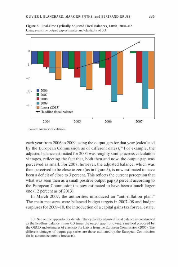
A small fiscal headline deficit turned into a small headline surplus in 2007. Was it the appropriate fiscal stance? This is where hindsight comes heavily into play. As of 2007, the European Commission’s assessment was that Latvia’s output was only slightly above potential, so the output gap was perceived to be only slightly positive. In hindsight, it has become clear that the output gap was in fact larger, and thus the “cyclically adjusted” fiscal balance was much worse. Fiscal policy was procyclical. The point is illustrated in figure 5, which plots the cyclically adjusted balance for
2000 = 100
120
160
200
240
2000 2002 2004 2006 2008 2010 2012
CPI
GDP deflator
ULC Export price deflator
Source: Authors’ calculations.
Figure 4. Price deflators and unit labor cost, latvia, 2000–12
9. Eurostat official data on house prices start only in 2006; even so, from 2006Q1 until the peak in 2008Q1 they show a 75 percent increase.
Olivier J. Blanchard, Mark Griffiths, and Bertrand Gruss 335
each year from 2006 to 2009, using the output gap for that year (calculated by the European Commission as of different dates).10 For example, the adjusted balance estimated for 2004 was roughly similar across calculation vintages, reflecting the fact that, both then and now, the output gap was perceived as small. For 2007, however, the adjusted balance, which was then perceived to be close to zero (as in figure 5), is now estimated to have been a deficit of close to 3 percent. This reflects the current perception that what was seen then as a small positive output gap (3 percent according to the European Commission) is now estimated to have been a much larger one (12 percent as of 2013).
In March 2007, the authorities introduced an “anti-inflation plan.” The main measures were balanced budget targets in 2007–08 and budget surpluses for 2009–10, the introduction of a capital gains tax for real estate,
10. See online appendix for details. The cyclically adjusted fiscal balance is constructed as the headline balance minus 0.3 times the output gap, following a method proposed by the OECD and estimates of elasticity for Latvia from the European Commission (2005). The different vintages of output gap series are those estimated by the European Commission (in its autumn economic forecasts).
–4
–3
–2
–1
0
2004 2005 2006 2007
2006200720082009Latest (2013)Headline fiscal balance
Source: Authors’ calculations.
Figure 5. real-time cyclically adjusted fiscal Balances, latvia, 2004–07 Using real-time output gap estimates and elasticity of 0.3
336 Brookings Papers on Economic Activity, fall 2013
and attempts to restrain bank lending (including making loans exclu-sively on clients’ legal incomes as opposed to their stated incomes, making 10 percent first-installment payments mandatory, and fixing a maximum loan-to-value ratio). However, it was too little too late.11
In short, the anticipation of a large scope for catch-up growth, together with cheap external financing, led to an initially healthy boom. As time passed, the boom turned unhealthy, with overheating leading to appreciation and large current account deficits, along with lower credit quality and the balance sheet risks associated with foreign exchange borrowing.
It is no great surprise that the government was reluctant to acknowledge the changing nature of the boom and thus was unwilling to slow it down dramatically. As late as mid-2006, government officials argued that macro-economic developments were largely benign: rapid growth was essential for income convergence, inflation was due more to wage and price con-vergence than to demand factors, and increased infrastructure investment would prevent growth bottlenecks and enhance competition. In the words of the then transport minister, it was time to “put the pedal to the metal.”12 The financial regulator saw potential for further credit growth, arguing that household debt ratios were low and that the strong and liquid housing market provided adequate loan collateral. The regulator regarded its responsibility to be one of ensuring that individual banks had sufficient capital rather than one of playing a macroprudential role. In contrast, the Bank of Latvia appeared more concerned about overheating and the risks from high debt levels and large currency and real estate exposures. Although it supported fiscal tightening, aside from raising reserve requirements the Bank of Latvia lacked the instruments to respond, given the quasi currency board and the open capital account.
An interesting question, with obvious implications beyond Latvia, is whether outside observers with no obvious political stake were sounding the alarm bell more strongly than the Latvian authorities. The answer, at least in the case of the IMF, is a qualified yes. In its 2005 annual review
11. Ending the practice of allowing borrowers to state fictitious incomes and imposing maximum loan-to-value ratios did help stop the demand for real estate, nevertheless. And when prices started to fall, demand dried up, anticipating future price declines.
12. “The Latvian government didn’t do much to stop this economic transformation. If anything, it stepped on the gas. Riga’s new deputy mayor and millionaire Ainars Slesers, who served in the Latvian Parliament during the boom years, coined a phrase that is sure to become a symbol of the prevailing government attitude at the time: gazi grida (pedal to the metal).” From “Latvia’s Tiger Economy Loses Its Bite,” a journalistic report by Kristina Rizga published online by the Pulitzer Center on Crisis Reporting, http://pulitzercenter.org/articles/latvias-tiger-economy-loses-its-bite.

Olivier J. Blanchard, Mark Griffiths, and Bertrand Gruss 337
(the so-called Article IV review), the IMF pointed out problems arising from rapid credit growth and domestic banks’ increasing reliance on non-resident deposits for funding. It viewed the authorities’ decision to remove limits on banks’ open positions in euros (because of the peg and the goal of euro adoption) as premature. In 2006, the IMF renewed its warnings, recommending stronger fiscal tightening and macroprudential measures to limit credit. In its concluding statement for the 2007 Article IV mission, its warnings were even more explicit.
The record of credit agencies was definitely mixed. Though they low-ered their outlooks, ratings agencies were slow to react with ratings down-grades. For example, while Moody’s recognized that rising inflation and current account deficits posed risks, it cited as mitigating factors the gov-ernment’s low debt ratio and stable external funding of the financial system (long-term loans from parent banks plus nonresident deposits, which it viewed as stable). Standard & Poor’s (S&P) kept its A– rating until May 2007 and then kept its BBB+ until October 2008. Fitch kept an A– rating until August 2007 and then a BBB+ until October 2008. Moody’s kept its A2 rating until November 2008. S&P and Fitch did not lower their ratings to BB+ (below investment grade) until February and April 2009, respectively, while Moody’s kept its investment grade rating throughout.
II. On the Bust, Part 1: Fatigue and the Global Financial Crisis
The boom ended in two distinct phases. First there was a slowdown, before the global financial crisis. Then came a collapse due to the impact of the crisis, through a sudden stop of capital inflows, a credit crunch, and a sharp drop in exports.
II.A. Fatigue and the Slowdown
Booms sometimes die a natural death. The stock adjustment process that initially increased investment and durable consumption comes to an end. Expectations of sustained fast growth turn out to be too optimistic and are revised downward, leading to lower domestic demand. Credit quality deteriorates, leading banks eventually to tighten credit. Increasing wage and price inflation lead to increasing overvaluation and reduced exports.
In Latvia the first signs of such fatigue appeared in 2006. Consumer confidence peaked in 2006Q3, and business confidence peaked in 2007Q1. Then, starting in February 2007, worries about the exchange rate peg led to a large jump in the Rigibor, the Latvian interbank rate, relative to its Euribor counterpart, with the spread increasing from 0.5 percent to 6 percent

338 Brookings Papers on Economic Activity, fall 2013
within two months. By early 2007, credit standards were being tightened, led by subsidiaries of Swedish banks. Borrowing rates rose from around 7 percent at the start of the year to peak at around 15 percent in November—although, as discussed earlier, real interest rates declined because of the sharp increase in inflation. Output peaked in 2007Q4.
Had there been no global financial crisis, Latvia might have gone through a slump similar in nature to what happened in Portugal in the early 2000s: weak foreign demand due to the overvaluation triggered by the earlier boom and weak domestic demand, due in part to tighter credit.13 However, starting in 2008 this adjustment process was overtaken by the effects of the world financial crisis.
II.B. The Global Financial Crisis and the Bust
As in other emerging markets, the global financial crisis affected Latvia through two main channels: trade and financial.14
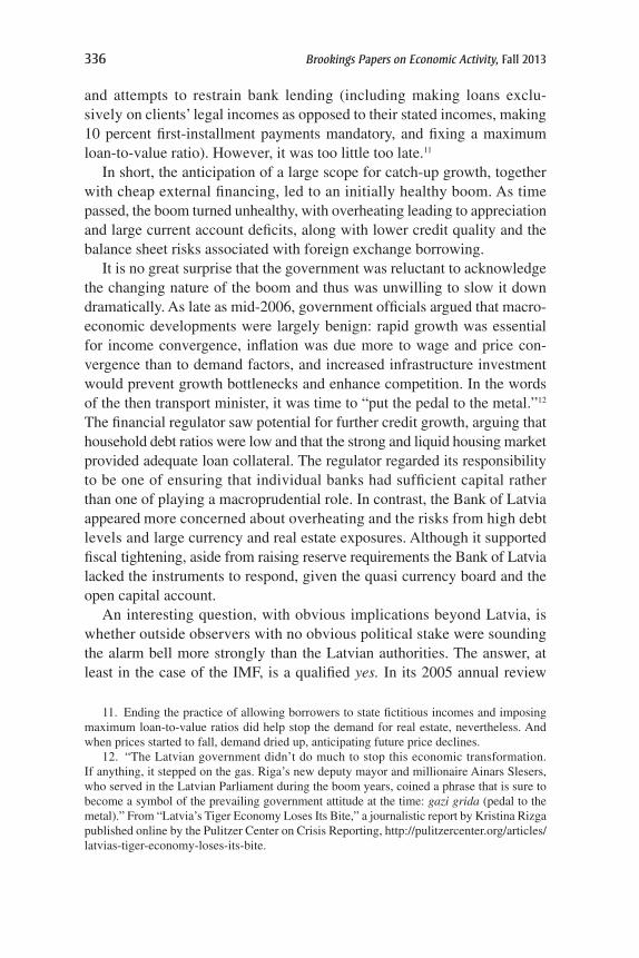
It is useful to look at the evolution of the different components of GDP during the bust. Figure 6 shows the evolution of each component of GDP from the peak in 2007Q4 to the trough in 2009Q3 as a percentage of 2007Q4 GDP.
Over those eight quarters, GDP declined by 25 percent. Foreign demand (X) accounted for 8 percent of the decrease. But much more dramatic was the decrease in domestic demand (C+I+G), which declined by 43 percent of GDP! Fixed investment itself fell by more than half. This decrease in domestic demand was partly offset in its effect on the demand for domestic goods—and by implication in its effect on GDP—by a decrease in imports (M) of 26 percent of GDP.15 These numbers have a clear implication: The bust was due in part to a decrease in foreign demand, but much more so to a collapse in domestic demand.
Looking more closely, we start by examining foreign demand. Exports started declining in 2008Q1, while world demand was still increasing, before the global crisis. This decrease was probably due to the increasing over-valuation noted earlier. But the major decline took place during 2008Q4 and 2009Q1. During those two quarters, exports fell by 8 percent of GDP, clearly due to the global crisis.
13. On Portugal, see Blanchard (2007) and Reis (2013).14. A first pass at the effects of the crisis on emerging market economies in general was
presented in an earlier Brookings Paper (Blanchard, Das, and Faruqee 2010).15. The decrease in imports seems large as a proportion of GDP, but the relevant denomi-
nator is domestic demand. The decrease in imports is equal to 60 percent of the decrease in domestic demand, roughly equal to the ratio of imports to domestic demand in 2008:1.
Olivier J. Blanchard, Mark Griffiths, and Bertrand Gruss 339
Dynamic simulations, using an estimated export equation specifying log exports as a function of the log of the partner countries’ GDP (using trade weights) and the real exchange rate, suggest that the adjustment was faster than usual, but by 2009Q2 they were roughly in line with what would have been predicted.16
How much of the decrease in output can be explained by the decrease in foreign demand? About 30 percent of exports are re-exports. So a decrease in exports of 8 percent of GDP implies a decrease in net external demand of just over 5 percent. In our earlier BPEA paper on emerging markets during the crisis (Blanchard, Das, and Faruqee 2010), we found that an (unexpected) decrease in exports of 1 percent of GDP led to a 1.5 percent (unexpected) decrease in GDP; applying that finding to this case, we arrive at (5 × 1.5 =) 7.5 percent. Given the size of the decrease in domestic demand (43 percent), it is clear that the dominant factors must be found elsewhere, namely with the credit crunch and the sudden stop, starting in 2008; fiscal policy did not play much of a role until the middle of 2009. We discuss the sudden stop and credit crunch as well as the role of fiscal policy in the next two sections.
–25
–20
–15
–10
–5
0
2008Q1 2008Q3 2009Q1 2009Q3
Exports
Investment
Consumption
GDP
Imports
Percent of 2007Q4 real GDP
Source: Authors’ calculations.
Figure 6. evolution of GdP components during the crisis, latvia, 2007Q4–2009Q3
16. See online appendix. The estimated elasticity with respect to partner country GDP is 1.58; the estimated elasticity with respect to the real exchange rate is -0.21.
340 Brookings Papers on Economic Activity, fall 2013
III. The Bust, Part 2: The Sudden Stop and the Credit Crunch
The relative simplicity of the Latvian financial system makes it easier to trace the effects of the sudden stop.
Some background is in order. In 2008, Latvian subsidiaries of Nordic banks accounted for 60 percent of total bank assets.17 The largest domes-tic bank, Parex, accounted for another 14 percent. Other domestic banks accounted for the remaining 26 percent. The banks had different busi-ness models. On the liability side, the Nordic subsidiaries were financed 1⁄3 by resident deposits and 2⁄3 by their parent banks. In contrast, Parex was financed in roughly equal proportions by resident and nonresident deposits, most of the latter from the recently independent eastern European nations (the CIS countries).18 Thus, funding for the Nordic banks depended very much on the decisions of their parent banks, and funding for Parex depended on the behavior of nonresident depositors and lenders from abroad.
As noted earlier, credit growth had already slowed before the global crisis. New loans had peaked in 2006Q4 (and therefore before the decrease in output), and real credit growth had slowed from 12 percent (quarter on quarter) in 2006Q4 to being virtually flat one year later. But the trigger for the financial crisis was a run on Parex in the wake of the Lehman collapse.
Parex was exposed to high rollover risk. In addition to funding by non-resident deposits, large syndicated loans, amounting to 16 percent of its end-2008 liabilities, would be coming due in early 2009, and a eurobond, accounting for another 4 percent of its liabilities, was potentially callable, for example in the event of default on syndicated loans. In contrast to the Nordic subsidiaries, Parex had no parent bank and therefore no deep pockets. And under a currency board, there was, at least in principle, no room for liquidity provision by Latvia’s central bank.
A “bank walk” started in late July 2008. Then, starting in early October (a few weeks after the Lehman collapse), the walk turned into a run. By the end of 2008, total deposits in Parex were down by 34 percent relative to June. Various measures were taken by the Latvian supervisory authority and by the government. A partial public takeover in November was followed by full nationalization later in the month. However, even this did not stop the run. Restrictions on deposit withdrawals from Parex had to be imposed in early December 2008.
17. Latvian subsidiaries of Nordic banks include Swedbank, SEB, DNB, Danske Bank, and Nordea (the last two operate as branches rather than as subsidiaries).
18. Nonresident deposits in Latvia were mostly by CIS corporations, due to ease of transaction, geographical proximity, and language.
Olivier J. Blanchard, Mark Griffiths, and Bertrand Gruss 341
As nonresidents closed their accounts and converted them into foreign currency or moved their money outside the country, the central bank defended the peg. Reserves fell (ignoring valuation effects from the depreciation of the euro and thus the lat). In the last three months of 2008, the Bank of Latvia sold €1.15 billion, or roughly one quarter of its end-September reserves. Under a strict currency board, there would have been no further central bank intervention, which would have implied a decrease in the monetary base equal to the decrease in reserves. However, there was strong pressure to provide funds to Parex. This was eventually done, though indirectly. The government placed Treasury bills and increased Treasury deposits at Parex (to one-third of total deposits by end-2008), which in turn used the bills to obtain financing from the central bank to fund deposit outflows. In turn, international donors—at first a swap line from the Swedish and Danish central banks, which served as a bridge to a subsequent IMF/EU/Nordic program—replenished the reserves of the central bank.
Fortunately for Latvia’s economy, the Nordic parent banks absorbed losses by recapitalizing their subsidiaries and committing to not cut funding to their subsidiaries, both implicitly at the start of the program and more formally later on. Loans from these Latvian subsidiaries to residents still declined, from a peak of 10.5 billion lats in 2008Q4 to 8.1 billion lats at the end of 2011, but it was a smooth decline, and it is likely that much of it could be explained by lower credit demand rather than by the tighter credit supply alone.
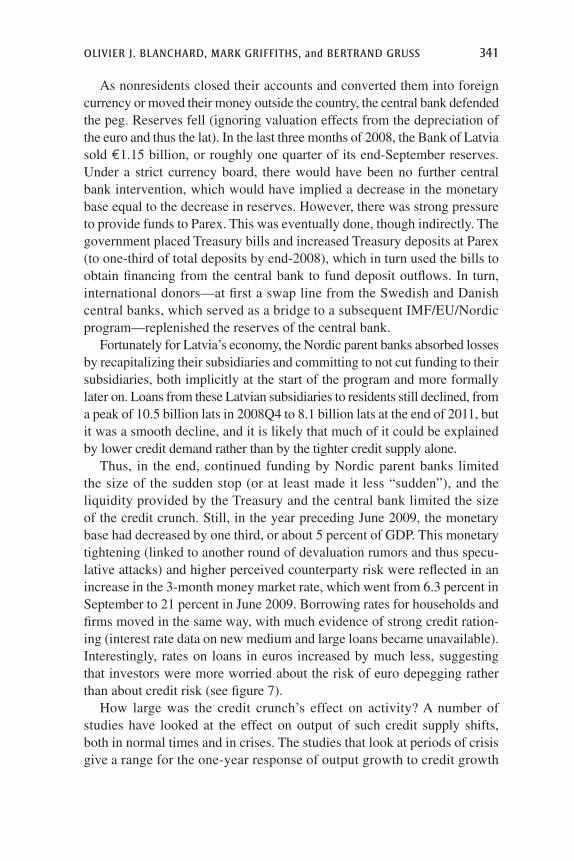
Thus, in the end, continued funding by Nordic parent banks limited the size of the sudden stop (or at least made it less “sudden”), and the liquidity provided by the Treasury and the central bank limited the size of the credit crunch. Still, in the year preceding June 2009, the monetary base had decreased by one third, or about 5 percent of GDP. This monetary tightening (linked to another round of devaluation rumors and thus specu-lative attacks) and higher perceived counterparty risk were reflected in an increase in the 3-month money market rate, which went from 6.3 percent in September to 21 percent in June 2009. Borrowing rates for households and firms moved in the same way, with much evidence of strong credit ration-ing (interest rate data on new medium and large loans became unavailable). Interestingly, rates on loans in euros increased by much less, suggesting that investors were more worried about the risk of euro depegging rather than about credit risk (see figure 7).
How large was the credit crunch’s effect on activity? A number of studies have looked at the effect on output of such credit supply shifts, both in normal times and in crises. The studies that look at periods of crisis give a range for the one-year response of output growth to credit growth
342 Brookings Papers on Economic Activity, fall 2013
of 0.3 to 1.1.19,20 This suggests the following back-of-the-envelope com-putation: Loan growth from 2008Q3 (when loans peaked) to 2009Q3, in real terms, was around -5 percent, compared to loan growth over the four quarters up to 2008Q3 of around 3 percent (already down from close to 50 percent 18 months earlier). The parameters above suggest that this decrease in loan growth of 8 percent may explain a decrease in domestic demand growth between 3 and 9 percent.21 This is a large decline, but it is
5
10
15
20
2008 2009 2010 2011
Mortgage rate, lats
Mortgage rate, euros
Firms (small loans), lats
Firms (small loans), euros
Percent
Source: Authors’ calculations.
Figure 7. interest rates during the crisis (new loans), latvia, 2008–11
19. Calomiris and Mason (2003) focus on the Great Depression; Peek and Rosengren (2000) on Japan; Greenlaw and others (2008) and Duchin, Ozbas, and Sensoy (2010) on this crisis; and Claessens, Kose, and Terrones (2009) on a number of crunches.
20. It is not clear whether the right parameter one should look at is the response of output growth to credit growth, or instead the response of output growth to the change in the credit-to-GDP ratio. The studies’ results that we mention are stated in terms of the first.
21. It is not clear that credit growth is the right metric to relate to demand growth. As one might expect, the decrease in new loans was much larger. After peaking in 2006Q4, the flow of new loans (constructed from the change in the credit stock and an estimated amortization flow based on the maturity structure of bank loans) had decreased by 65 percent in real terms by end-2008 and by 85 percent by end-2009. A related metric, constructed as the difference in the flow of credit relative to GDP (see Biggs, Mayer, and Pick 2009) would suggest that the contribution of credit to demand growth, or credit impulse, was -19 percent of GDP over the period 2008Q3 to 2009Q3.
Olivier J. Blanchard, Mark Griffiths, and Bertrand Gruss 343
still substantially less than the decrease in domestic demand of 27 per-cent over the same period.
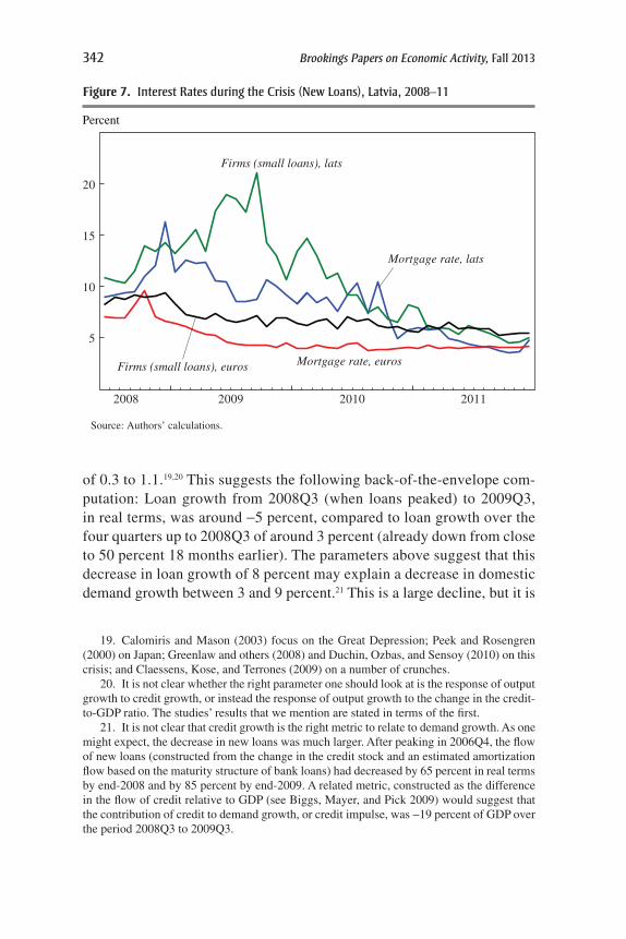
So what else can explain the collapse in demand? By process of elimina-tion, the answer seems to be uncertainty and the option value of waiting. Suggestive evidence is given by the behavior of car sales during the period. As shown in figure 8, new car registrations, normalized to be 100 in 2007, collapsed to 18 in January 2009 and fell gradually during the year to reach one tenth of their 2007 levels by January 2010.22,23 Some of the decrease came from credit rationing: Partly because of the general uncertainty, and partly because of legal uncertainty about the ability of banks to repossess the collateral, banks simply stopped offering car loans. But much of the precipitous drop in car sales clearly came from the high uncertainty facing consumers, be it about the peg, the soundness of the banking system, or the size of the ongoing recession.
2007 = 100
40
80
120
2005 2007 2009 2011 2013
Source: Authors’ calculations.
Figure 8. new car registrations, latvia, 2005–13
22. For comparison, in her study of the effects of uncertainty on spending at the onset of the Great Depression, Christina Romer (1990) found that car registrations declined by 24 percent from September 1929 to January 1930.
23. Anecdotally, Latvia, which does not produce cars, became a car exporter for a few months in late 2009 and early 2010, as dealers, unable to sell their inventory of cars at home, sold them to foreign dealers.
344 Brookings Papers on Economic Activity, fall 2013
IV. On Adjustment Choices: Fiscal Consolidation
In early 2009, after the large decrease in output, what was needed to return Latvia to health? Again, it is important to keep in mind the two sources of the crisis: the natural (or unnatural) end of a boom, and the later collapse due to the world financial crisis. The world financial crisis had led to a sudden stop and a credit crunch, a large drop in exports, and a resulting large decrease in output. Recovery of the world economy would be needed to resolve the second source of the crisis. Financial cleanup would be needed to repair the first.
It was clear, however, that even without the financial crisis, Latvia would have needed a large macro adjustment. Latvia had been operating above potential output before the crisis. The resulting accumulated inflation had led to overvaluation, reflected in an unusually large current account deficit. And while the fiscal deficit had remained small, to return the fiscal deficit to balance at anything close to potential output would require substantial consolidation.
Many economists recommended a nominal devaluation, with some vari-ations, and a steady but smooth fiscal adjustment. (The variations included a one-time devaluation and then use of the ERM II bands, backed by the potential support of ECB intervention, or even an accelerated adoption of the euro). The argument in favor of devaluation was an old one, namely that external devaluations solve a coordination problem and are easier to achieve than internal devaluations: A nominal exchange rate adjustment automatically coordinates real price and wage adjustments. The argument in favor of a steady but smooth fiscal adjustment was that the increase in the deficit was mostly due to the crisis and would largely go away as output recovered, combined with the point that the ratio of net debt to GDP, while it would likely increase because of bank recapitalization costs and future budget deficits, was still very low at end-2008, at less than 15 percent.
The Latvian government, and especially the Bank of Latvia, rejected this advice, deciding instead to maintain the peg and proceed with front-loaded consolidation. The authorities worried that depreciation would lead to inflation, and that the increase in the real value of foreign currency–denominated liabilities would lead to widespread insolvencies. They saw a devaluation as inconsistent with the goal of euro adoption, a goal delayed first by the boom (because of the induced inflation) and then by the crisis. They believed that institutional features (shallow financial markets, lack of offshore lats markets, difficulties for speculators to borrow in lats) reduced the risk of a speculative attack and made it more feasible to sustain the peg,
Olivier J. Blanchard, Mark Griffiths, and Bertrand Gruss 345
provided there was international financial support. They also believed that only a strong fiscal consolidation would send the signal that the government was committed to fiscal sustainability (see Åslund and Dombrovskis 2011).
The European Union, the European Central Bank, and the Nordic author-ities supported that strategy, albeit for their own reasons, including worries about contagion. While views within the IMF differed, it is fair to say that the IMF was more skeptical about the choice to maintain the peg but went along with the overall strategy.
The remainder of this section looks at the fiscal consolidation, and the next section looks at the adjustment under the peg—the so-called internal devaluation.
In 2008, the headline general government balance turned from a small surplus to a large deficit of 3.4 percent of GDP (excluding bank restructuring costs of around 4 percent of GDP), reflecting the large decrease in activity. Little fiscal consolidation took place until 2009, which is why in this study we did not focus on fiscal policy when explaining the initial decline in output.
A revised 2009 budget, passed in December 2008, included measures adding up to 7 percent of GDP—although some estimates suggest only 4 percent was actually implemented.24 In February 2009 the government fell, and in March a new government was put in place, with the challenge of implementing the fiscal consolidation that the previous government had agreed to but been unable to deliver (and which in part had caused its downfall). At the same time, the deepening recession was blowing the deficit wide open.
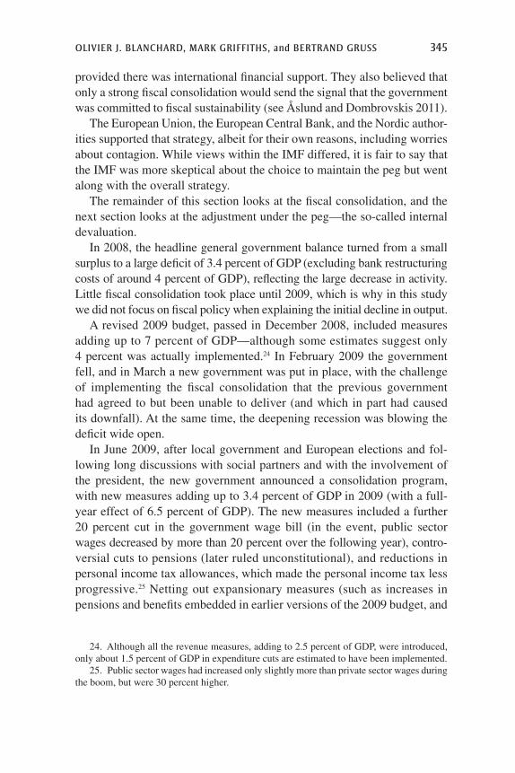
In June 2009, after local government and European elections and fol-lowing long discussions with social partners and with the involvement of the president, the new government announced a consolidation program, with new measures adding up to 3.4 percent of GDP in 2009 (with a full-year effect of 6.5 percent of GDP). The new measures included a further 20 percent cut in the government wage bill (in the event, public sector wages decreased by more than 20 percent over the following year), contro-versial cuts to pensions (later ruled unconstitutional), and reductions in personal income tax allowances, which made the personal income tax less progressive.25 Netting out expansionary measures (such as increases in pensions and benefits embedded in earlier versions of the 2009 budget, and
24. Although all the revenue measures, adding to 2.5 percent of GDP, were introduced, only about 1.5 percent of GDP in expenditure cuts are estimated to have been implemented.
25. Public sector wages had increased only slightly more than private sector wages during the boom, but were 30 percent higher.

346 Brookings Papers on Economic Activity, fall 2013
the approval of additional spending of 1 percent of GDP in social safety nets, as part of the program) and the likely partial implementation of earlier measures, fiscal consolidation in 2009 is estimated to have been about 8 percent of GDP; of this amount, only about 2 to 3 percent of GDP took effect in the first half of the year. These measures and others introduced in subsequent budgets implied a further adjustment of 5.4 percent of GDP in 2010 and 2.3 percent in 2011.
The evolution of headline deficits and of “cyclically adjusted” fiscal balances (our motivation for using quote marks will be clear below) from 2008 on is illustrated in figure 9. We plot three series: the change in the headline deficit, the change in the cyclically adjusted deficit including bank restructuring costs, and the change in the cyclically adjusted deficit exclud-ing bank restructuring costs.26
Percent of GDP
–6
–4
–2
0
2
4
2008 2009 2010 2011
Headline (change, excl. bank restructuring costs)Cyclically adjusted (change, excl. bank restructuring costs)Cyclically adjusted (change, incl. bank restructuring costs)
Source: Authors’ calculations.a. Changes measured using latest EC output gap estimates.
Figure 9. fiscal impulse: change in headline and cyclically adjusted Balances,a latvia, 2008–11
26. The cyclically adjusted fiscal balance in figure 9 is defined as the headline balance-to-GDP ratio minus the output gap times an overall budgetary sensitivity parameter, based on European Commission (2005) estimates, of 0.3.
Olivier J. Blanchard, Mark Griffiths, and Bertrand Gruss 347
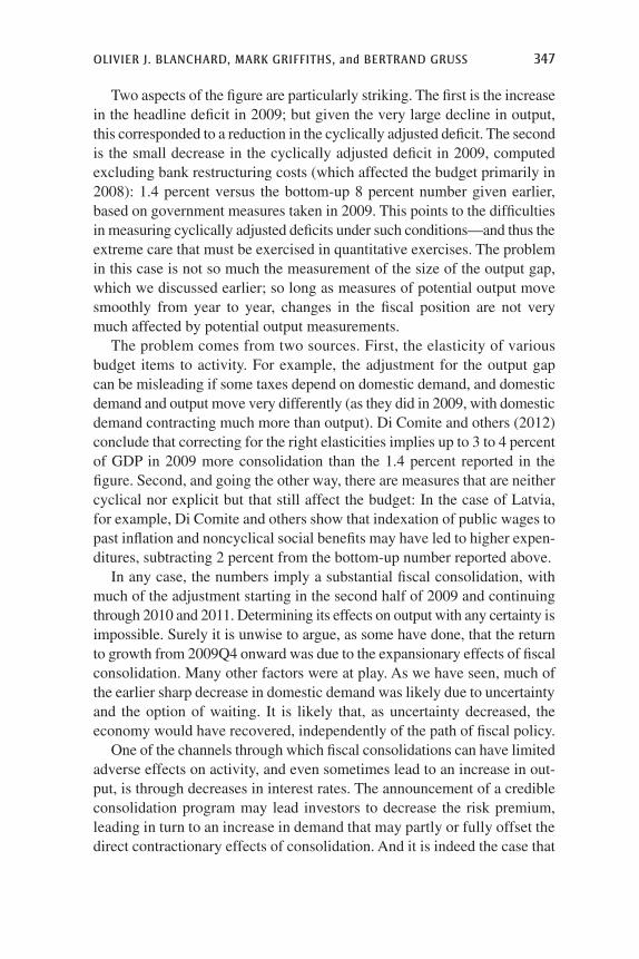
Two aspects of the figure are particularly striking. The first is the increase in the headline deficit in 2009; but given the very large decline in output, this corresponded to a reduction in the cyclically adjusted deficit. The second is the small decrease in the cyclically adjusted deficit in 2009, computed excluding bank restructuring costs (which affected the budget primarily in 2008): 1.4 percent versus the bottom-up 8 percent number given earlier, based on government measures taken in 2009. This points to the difficulties in measuring cyclically adjusted deficits under such conditions—and thus the extreme care that must be exercised in quantitative exercises. The problem in this case is not so much the measurement of the size of the output gap, which we discussed earlier; so long as measures of potential output move smoothly from year to year, changes in the fiscal position are not very much affected by potential output measurements.
The problem comes from two sources. First, the elasticity of various budget items to activity. For example, the adjustment for the output gap can be misleading if some taxes depend on domestic demand, and domestic demand and output move very differently (as they did in 2009, with domestic demand contracting much more than output). Di Comite and others (2012) conclude that correcting for the right elasticities implies up to 3 to 4 percent of GDP in 2009 more consolidation than the 1.4 percent reported in the figure. Second, and going the other way, there are measures that are neither cyclical nor explicit but that still affect the budget: In the case of Latvia, for example, Di Comite and others show that indexation of public wages to past inflation and noncyclical social benefits may have led to higher expen-ditures, subtracting 2 percent from the bottom-up number reported above.
In any case, the numbers imply a substantial fiscal consolidation, with much of the adjustment starting in the second half of 2009 and continuing through 2010 and 2011. Determining its effects on output with any certainty is impossible. Surely it is unwise to argue, as some have done, that the return to growth from 2009Q4 onward was due to the expansionary effects of fiscal consolidation. Many other factors were at play. As we have seen, much of the earlier sharp decrease in domestic demand was likely due to uncertainty and the option of waiting. It is likely that, as uncertainty decreased, the economy would have recovered, independently of the path of fiscal policy.
One of the channels through which fiscal consolidations can have limited adverse effects on activity, and even sometimes lead to an increase in out-put, is through decreases in interest rates. The announcement of a credible consolidation program may lead investors to decrease the risk premium, leading in turn to an increase in demand that may partly or fully offset the direct contractionary effects of consolidation. And it is indeed the case that
348 Brookings Papers on Economic Activity, fall 2013
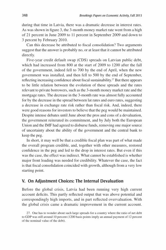
during that time in Latvia, there was a dramatic decrease in interest rates. As was shown in figure 3, the 3-month money market rate went from a high of 21 percent in June 2009 to 11 percent in September 2009 and down to 3 percent by February 2010.
Can this decrease be attributed to fiscal consolidation? Two arguments suggest that the answer is probably no, or at least that it cannot be attributed directly.
Five-year credit default swap (CDS) spreads on Latvian public debt, which had increased from 800 at the start of 2009 to 1200 after the fall of the government, indeed fell to 700 by the end of April, when the new government was installed, and then fell to 500 by the end of September, reflecting increasing confidence about fiscal sustainability.27 But there appears to be little relation between the evolution of these spreads and the rates relevant to private borrowers, such as the 3-month money market rate and the mortgage rates. The decrease in the 3-month rate was almost fully accounted for by the decrease in the spread between lat rates and euro rates, suggesting a decrease in exchange rate risk rather than fiscal risk. And, indeed, there were good reasons for investors to believe that the peg would be maintained. Despite intense debates until June about the pros and cons of a devaluation, the government reiterated its commitment, and by July both the European Union and the IMF had agreed to disburse funds, removing one major source of uncertainty about the ability of the government and the central bank to keep the peg.
In short, it may well be that a credible fiscal plan was part of what made the overall program credible, and, together with other measures, restored confidence in the peg and led to the drop in interest rates. But even if this was the case, the effect was indirect. What cannot be established is whether major front loading was needed for credibility. Whatever the case, the fact is that fiscal consolidation coincided with growth, although from a very low starting point.
V. On Adjustment Choices: The Internal Devaluation
Before the global crisis, Latvia had been running very high current account deficits. This partly reflected output that was above potential and cor respondingly high imports, and in part reflected overvaluation. With the global crisis came a dramatic improvement in the current account.
27. One has to wonder about such large spreads for a country where the ratio of net debt to GDP was still around 10 percent (1200 basis points imply an annual payment of 12 percent of the nominal value of the debt).
Olivier J. Blanchard, Mark Griffiths, and Bertrand Gruss 349
While exports further decreased, domestic demand collapsed, leading to a collapse in imports. During 2009, the current account actually swung into surplus (although part of this reflected the recording of foreign bank loan losses as positive investment income).
This surplus was hardly good news, however. It was likely that with the return of output to potential—whatever the precise value of potential out-put was (a subject that will be discussed later)—the current account deficit would reappear. To maintain a balanced current account as growth came back, there would be a need for a real depreciation. Estimates varied, but it was generally believed that a significant real depreciation was needed. While many argued that a devaluation of the lat was the best solution, the authorities emphatically rejected this approach. They decided instead to adjust through an internal devaluation, an adjustment of nominal prices and wages, rather than adjusting the nominal exchange rate.
So how did it work?
V.A. The Evolution of Unit Labor Costs
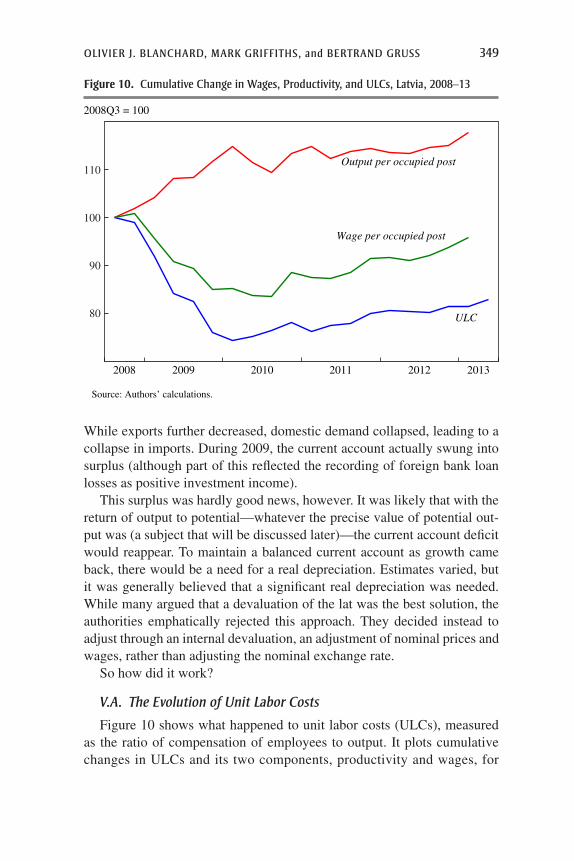
Figure 10 shows what happened to unit labor costs (ULCs), measured as the ratio of compensation of employees to output. It plots cumulative changes in ULCs and its two components, productivity and wages, for
2008Q3 = 100
80
90
100
110
2008 2009 2010 2011 2012 2013
ULC
Output per occupied post
Wage per occupied post
Source: Authors’ calculations.
Figure 10. cumulative change in Wages, Productivity, and ulcs, latvia, 2008–13
350 Brookings Papers on Economic Activity, fall 2013
the economy as a whole, from 2008Q3 on. (The decomposition of ULCs between productivity and wages requires the use of an employment series. As explained in the appendix, because of a break in the official employment series, we instead use “occupied posts,” that is, the number of employees as reported by firms.)
The evolutions are quite striking. The adjustment of ULCs was fast and substantial. By the end of 2009, ULCs had declined by close to 25 percent, and they have remained roughly stable since. While wage cuts played a role initially, much of the reduction in ULCs today reflects productivity improvements rather than wage cuts.
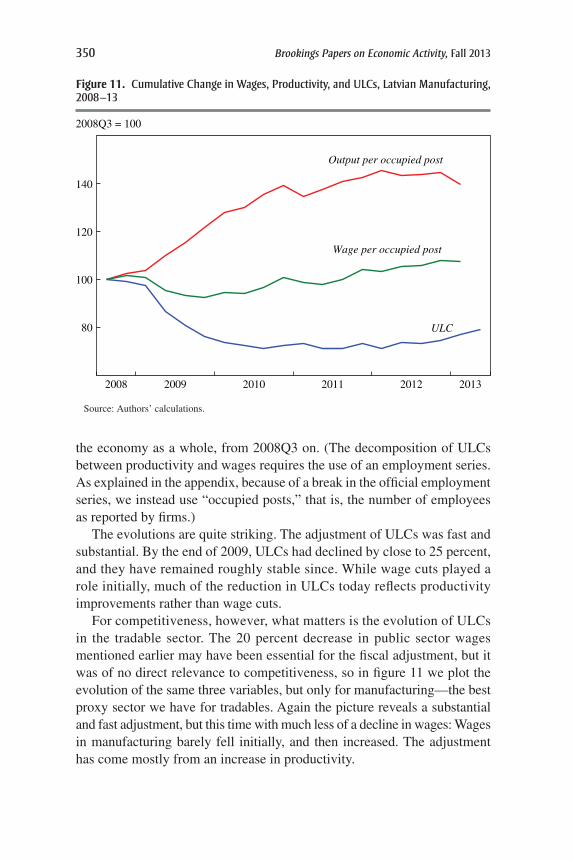
For competitiveness, however, what matters is the evolution of ULCs in the tradable sector. The 20 percent decrease in public sector wages mentioned earlier may have been essential for the fiscal adjustment, but it was of no direct relevance to competitiveness, so in figure 11 we plot the evolution of the same three variables, but only for manufacturing—the best proxy sector we have for tradables. Again the picture reveals a substantial and fast adjustment, but this time with much less of a decline in wages: Wages in manufacturing barely fell initially, and then increased. The adjustment has come mostly from an increase in productivity.
2008Q3 = 100
80
100
120
140
2008 2009 2010 2011 2012 2013
ULC
Output per occupied post
Wage per occupied post
Source: Authors’ calculations.
Figure 11. cumulative change in Wages, Productivity, and ulcs, latvian Manufacturing, 2008–13
Olivier J. Blanchard, Mark Griffiths, and Bertrand Gruss 351
What can explain this increase in productivity? Without question it was associated initially with labor shedding: Employment decreased in nearly all sectors, an outcome reflected in the large increase in unemployment. This raised the issue of whether the productivity improvement would be long lasting or whether it reflected something temporary, for example credit constraints forcing firms to take decisions they might reverse when credit improved. Events have shown that the latter does not appear to have been the case. Productivity gains have indeed remained, as figure 11 shows for manufacturing. Looking across subsectors within manufacturing, we find that productivity continued increasing even in subsectors where employment growth has resumed.
The question has been raised whether this increase in productivity reflects composition effects, namely that the decrease in employment was particularly pronounced for low-productivity sectors, or for low-productivity firms, or for low-productivity workers.28 Any such composition effect would lead to an overestimation of the true increase in productivity and therefore to an underestimation of the true decrease in wages. To examine sectoral composition effects, we constructed a fixed-weight wage series for the whole economy, using fixed employment shares for 110 NACE subsectors at the two-digit level;29 we found a less than 2 percent difference in the increase in the two series since 2008. To examine skill level composition effects, we looked at the relative employment of workers with only primary education. At a given unemployment rate (so comparing the unemploy-ment rate in 2004 to the unemployment rate today), these workers’ share in employment has indeed declined, from roughly 13 percent to 9 percent. Using the wage differential between them and other workers, this implies that skill composition effects may have led to an increase in the average wage of about 3 percent, again a small number.
This suggests that decreases in private sector wages have indeed been limited and that productivity increases have been genuine. That may be because tight credit constraints forced firms—and limited employment protection allowed them—to reduce some X-inefficiency built up in the boom. Or it may be, as Paul Krugman has argued, that underlying pro-ductivity growth was high and the increase in productivity was simply a return to the trend—if so, an option relevant for Latvia and other Baltic countries but much less so for southern periphery euro countries.
28. See, for example, Krasnopjorovs (2013).29. NACE is the European community’s statistical system for classifying economic activity.
Due to data availability, data at the one-digit level were used for (B) Mining and quarrying; (Q) Human health and social work activities; and (R) Arts, entertainment, and recreation.

352 Brookings Papers on Economic Activity, fall 2013
Before the adjustment started, one of the main worries was that large nominal wage cuts would be needed, and judging from the evidence from other advanced countries, that it would be a slow and difficult process at best (as it has indeed proven to be in euro countries on the southern periphery). The increase in productivity made this a less central worry, since all else being equal, smaller nominal wage cuts were needed. In fact, smaller nominal wage cuts were achieved.
Still, the large divergence between productivity and wages raises the question: Why were productivity gains not matched by wage increases? Clearly, the large increase in the unemployment rate, weaker unions, and limited employment protection must have all played a central role. Also playing a central role must have been the large decrease in public sector wages, which was part of the 2009 fiscal adjustment.30 Other factors, specific to Latvia, were also likely at play, although they are impossible to quantify. One is the earlier boom: Latvians probably knew that the earlier large wage increases were excessive. Looking at the Baltic and euro periphery countries, Joon Shik Kang and Jay Shambaugh (2013) find that countries that had greater wage increases during the boom (since 2000) had greater wage decreases later. Another factor likely at play was the still-recent history of Latvia, including its painful transition to a market economy in the early 1990s and the sense of national unity in the face of its Russian neighbor. Yet another likely factor was the determination to integrate more closely with Europe and join the eurozone.
V.B. From Unit Labor Costs to Prices
One would have expected the decrease in ULCs to be reflected in lower export prices and thus higher competitiveness. The story is more complicated, however.
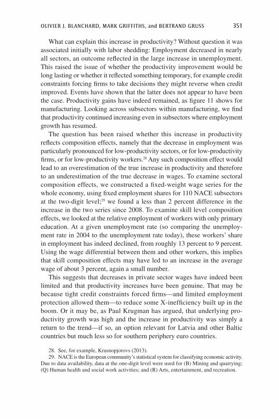
Figure 12 shows the evolution of manufacturing ULCs (used as a proxy for the ULCs in the export sector) since 2000. It also shows the corresponding evolution in export prices and a partner country price index (constructed as a weighted average of partner country import prices, using Latvian 2009–11 export shares as weights). Export prices did decline in 2009, but they generally moved in line with partner country prices—which themselves declined because of the global crisis. Indeed, the proportional decline in Latvia’s export prices was equal to the proportional decline in
30. See the next section and the online appendix for the results of estimation of Phillips curve relations. The time series is however too short to reach strong conclusions. A Phillips curve specification, allowing for an effect of public sector on private sector wage inflation, does not yield conclusive results. But it may be that there was a one-time strong effect in 2009.
Olivier J. Blanchard, Mark Griffiths, and Bertrand Gruss 353
the partner country price index. Thus, ULCs may have played a role, but it was a limited one. Since then, export prices have recovered, while ULCs have remained low. This suggests that Latvian exporters are largely price takers, with the implication that the decrease in ULCs has led more to an increase in profit margins than to lower prices in the export sector.31,32
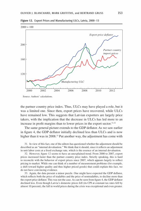
The same general picture extends to the GDP deflator. As we saw earlier in figure 4, the GDP deflator initially declined less than ULCs and is now higher than it was in 2008.33 Put another way, the adjustment has come with
2000 = 100
120
160
200
2000 2002 2004 2006 2008 2010 2012
Export price deflator
Partner country import prices
Manufacturing ULC
Source: Authors’ calculations.
Figure 12. export Prices and Manufacturing ulcs, latvia, 2000–13
31. In view of this fact, one of the editors has questioned whether the adjustment should be described as an “internal devaluation.” We think that it should, since it reflects an adjustment in unit labor costs at a fixed exchange rate, which is the essence of an internal devaluation.
32. However, figure 12 seems to have an unexplained trend. From 2000 to 2007, export prices increased faster than the partner country price index. Strictly speaking, this is hard to reconcile with the behavior of export prices since 2007, which appears largely to reflect pricing to market. While one can think of a number of measurement problems (for example, a shift toward higher quality and thus higher priced goods) that could explain this fact, we do not have convincing evidence.
33. Again, the data present a minor puzzle. One might have expected the GDP deflator, which reflects both the price of tradables and the price of nontradables, to decline more than the export price deflator. This was not the case. As can be seen from figure 4, the GDP deflator declined less. Even though Latvia’s domestic prices fell (its CPI at constant tax rates fell by almost 10 percent), the fall in world prices during the crisis was exceptional and even greater.
354 Brookings Papers on Economic Activity, fall 2013
a large drop in the labor share (recall that the labor share can be expressed as the ratio of the ULC to the GDP deflator). This is shown in figure 13, which plots the labor share both for the economy as a whole and for manu-facturing alone, starting in 2000.
For the economy as a whole, the labor share has fallen from 58 percent at the peak to 46 percent. For manufacturing, the share has gone from 64 percent to 45 percent. Figures 4 and 12 make clear that this is largely the mirror image of what had happened during the late part of the boom. Wages had increased faster than the GDP deflator, and the labor share had steadily increased. The adjustment has undone this increase—in the case of manufacturing, it has more than undone it.
In short: The adjustment of ULCs and prices was surprisingly fast. And in contrast to expectations and the textbook adjustment, it came largely from productivity increases and has been reflected more in larger profit margins rather than in lower prices.
V.C. External and Internal Demand
Increases in profit margins typically lead to a supply response, but it is generally believed that this response is slow. Exports, however, increased
2008Q3 = 100
45
50
55
60
2000 2002 2004 2006 2008 2010 2012
Whole economy
Manufacturing
Source: Authors’ calculations.
Figure 13. labor shares in Whole economy and Manufacturing, latvia, 2000–13
Olivier J. Blanchard, Mark Griffiths, and Bertrand Gruss 355
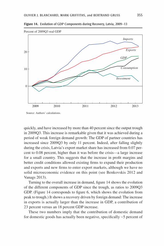
quickly, and have increased by more than 40 percent since the output trough in 2009Q3. This increase is remarkable given that it was achieved during a period of weak foreign demand growth: The GDP of partner countries has increased since 2009Q3 by only 11 percent. Indeed, after falling slightly during the crisis, Latvia’s export market share has increased from 0.07 per-cent to 0.08 percent, higher than it was before the crisis—a large increase for a small country. This suggests that the increase in profit margins and better credit conditions allowed existing firms to expand their production and exports and new firms to enter export markets, although we have no solid microeconomic evidence on this point (see Benkovskis 2012 and Vanags 2013).
Turning to the overall increase in demand, figure 14 shows the evolution of the different components of GDP since the trough, as ratios to 2009Q3 GDP. (Figure 14 corresponds to figure 6, which shows the evolution from peak to trough.) It shows a recovery driven by foreign demand: The increase in exports is actually larger than the increase in GDP, a contribution of 23 percent versus an 18 percent GDP increase.
These two numbers imply that the contribution of domestic demand for domestic goods has actually been negative, specifically -5 percent of
Percent of 2009Q3 real GDP
0
10
20
2009 2010 2011 2012 2013
Imports
Exports
GDP
Consumption
Investment
Source: Authors’ calculations.
Figure 14. evolution of GdP components during recovery, latvia, 2009–13

356 Brookings Papers on Economic Activity, fall 2013
GDP. Domestic demand itself has been reasonably strong, with increases in consumption and investment accounting for 13 percent and 6 percent of GDP, respectively. But imports have increased by a surprising 24 percent of GDP. If one removes that part of imports that is re-exported (about one-third of exports), the remaining increase in imports is still 17 percent of GDP (24 percent minus 0.3 times 23 percent), and therefore nearly equal to the increase in domestic demand—a surprisingly large increase. Part of the explanation must be a rebound from the exaggerated import collapse of 2009. Another, more intriguing explanation is the reversal of a phenom-enon analyzed by Rudolfs Bems and Julian Di Giovanni (2013), who, based on supermarket data during the bust, found that consumption had shifted toward lower quality and lower priced goods, which tended to be domestic goods. As income recovered, the reverse of this effect may have taken place.
V.D. Balance Sheet Effects, Investment, and Consumption
During the boom, as loans were increasingly being set in foreign currency, a growing worry (expressed, for example, in a number of IMF reports) was that the eventual adjustment would lead to strong adverse balance sheet effects. It is estimated that as of 2008, foreign exchange exposure amounted to 25 percent of GDP for consumers and 44 percent of GDP for firms. (Both the public sector—government and central bank consolidated—and banks had a small positive net foreign exchange position.) A back-of-the- envelope computation suggested that, for example, a 20 percent real deval-uation, whether achieved through external or internal devaluation, would reduce the net worth of consumers by 5 percent of GDP and the net worth of firms by 8.8 percent—holding GDP constant.34 Balance sheet effects could also come from declines in housing prices. Although only 25 percent of households had mortgages, a large decline in housing prices would lead to an increase in the number of households underwater. Mortgages in Latvia are full recourse and are often backed by the personal guarantees of family members. These adjustments could lead to large wealth effects and a large increase in the proportion of nonperforming loans, preventing the recovery (again, a worry that has proven to be relevant in a number of euro periphery countries).
34. While both internal and external devaluations imply the same foreign-exchange-induced balance sheet effects, their timing can be different. The balance sheet effect is instan-taneous in the case of a nominal exchange rate adjustment. But it happens over time in the case of an internal devaluation, and thus allows more time to adjust.
Olivier J. Blanchard, Mark Griffiths, and Bertrand Gruss 357
What, then, actually happened? Again, the script has deviated somewhat from the feared scenario and from the textbook. The fact that the adjust-ment has mostly taken the form of productivity increases rather than wage decreases has limited the increase in the ratio of nominal debt to wages. The fact that prices have adjusted less than wages have implies that bal-ance sheet effects have affected firms less than households. Housing prices, however, fell by half between 2008Q1 and 2010Q1 (private estimates suggest the decrease may have been as large as 70 percent).
The result of this has been an increase in nonperforming loans (NPLs), though the increase has been one the banks have been able to manage. Firms’ NPLs peaked at 22 percent of loans in early 2010, and as of mid-2013 were down to 8.5 percent. Households’ NPLs stabilized for some time at a high 20 percent, but have now decreased to 14.1 percent. There has been a sub-stantial restructuring of loans: about ¹⁄3 of the end-2009 stock of loans was restructured between 2010Q1 and 2013Q2. Cumulative write-offs during that period amounted to 7 percent of the end-2009 stock of loans. By June 2013, 10 percent of the stock of loans was still in the work-out process, 14 percent in the case of loans to households.
Despite the still high NPLs, the banking system is in decent shape and is profitable again. As of June 2013, Latvian banks reported a capital adequacy ratio of 18.6 percent, up from 11 percent at end-2007 and 14.6 percent at end-2009, and 71 percent of NPLs were provisioned. Parex no longer exists; it was recapitalized through a conversion of the Treasury deposits into equity and subordinated debt in May 2009 and then split into a “good bank/bad bank” in August 2010. Core assets and some non-core performing assets were transferred to a new bank, Citadele Bank. Remaining assets and liabilities were put in a special-purpose vehicle in March 2012. Except for Parex and a small public bank, MLB, the banking system received no public help.35
VI. Is Most of the Adjustment Complete?
Have the macro and financial adjustments been achieved? On the one hand, output has increased by 18 percent since the trough, the current account and the fiscal accounts are roughly in balance, and the financial system seems to be in decent shape. On the other hand, output is still 11 percent below its
35. More recently, Latvijas Krajbanka, a medium-size bank, had an intervention in November 2011 after fraud was discovered. But the bank did not receive state aid and was liquidated in early 2012.
358 Brookings Papers on Economic Activity, fall 2013
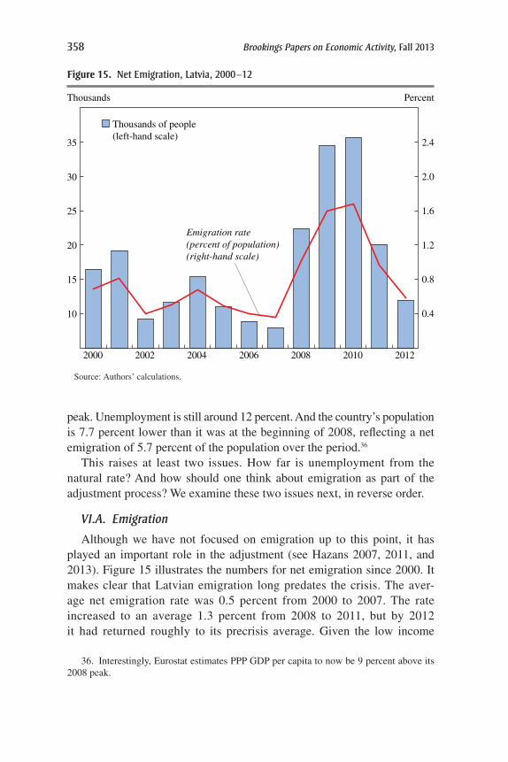
peak. Unemployment is still around 12 percent. And the country’s population is 7.7 percent lower than it was at the beginning of 2008, reflecting a net emigration of 5.7 percent of the population over the period.36
This raises at least two issues. How far is unemployment from the natural rate? And how should one think about emigration as part of the adjustment process? We examine these two issues next, in reverse order.
VI.A. Emigration
Although we have not focused on emigration up to this point, it has played an important role in the adjustment (see Hazans 2007, 2011, and 2013). Figure 15 illustrates the numbers for net emigration since 2000. It makes clear that Latvian emigration long predates the crisis. The aver-age net emigration rate was 0.5 percent from 2000 to 2007. The rate increased to an average 1.3 percent from 2008 to 2011, but by 2012 it had returned roughly to its precrisis average. Given the low income
Thousands Percent
10
15
20
25
30
35
0.4
0.8
1.2
1.6
2.0
2.4
2000 2002 2004 2006 2008 2010 2012
Thousands of people (left-hand scale)
Emigration rate (percent of population) (right-hand scale)
Source: Authors’ calculations.
Figure 15. net emigration, latvia, 2000–12
36. Interestingly, Eurostat estimates PPP GDP per capita to now be 9 percent above its 2008 peak.

Olivier J. Blanchard, Mark Griffiths, and Bertrand Gruss 359
per capita, and the fact that Latvia is part of the Schengen agreement on the free circulation of persons within the European Union, such steady emigration is easily explained. Nevertheless, the crisis clearly led to a temporarily higher emigration rate.37
What was the effect on unemployment? Two crude back-of-the-envelope computations give plausible upper and lower bounds. We can compute excess emigration as the increase in emigration in 2008–11 over the normal emigration trend, and thus as a cumulative 3.3 percent over four years. If we assume that, had they stayed, all the emigrants of working age would have remained unemployed, and given a ratio of the labor force to population of about 50 percent, the unemployment rate would be about 6 percent higher. Alternatively, if we assume that only those emigrants who were unemployed at the time of emigration had remained unemployed, but that the unemploy-ment rate among emigrants was 31⁄2 times higher than among non-emigrants, the unemployment rate would be about 3 percentage points higher.
The question, in either case, is whether this emigration reflects in some sense a failure of the adjustment program. In the United States, migration rather than unemployment is the major margin of adjustment to state-specific shocks (Blanchard and Katz 1992, with an update and extensions by Dao, Furceri, and Loungani 2013). These adjustments are typically regarded as good, indeed as the main reason why the United States functions well as a common currency area: If there are jobs in other states, and if moving costs are low, it is better for workers to move to those jobs than to remain unemployed.
Is the answer different for a small country than for a U.S. state? Some economic aspects are different: Some of the costs of running a country are fixed costs, and thus may not be easy to support with a smaller population. In the United States, many of those costs are picked up by the federal gov-ernment (although, as we have seen for Detroit, the remaining fixed costs per capita may make it difficult for a state or a city to function). This is not the case for a country, which must, for example, finance its defense budget alone. Political aspects may also be relevant, and a country may care more about the size of its population than does a U.S. state.
In that respect, an important question is who the emigrants are and whether they may return home. The evidence suggests that in Latvia the emigrants
37. Latvia’s implementation of the Schengen agreement started in December 2007, although Ireland, the United Kingdom, and Sweden opened their labor markets to those from the new EU member states in 2004. Thus, part of the post-2007 increase may also reflect easier access to labor markets in continental Europe.

360 Brookings Papers on Economic Activity, fall 2013
during the crisis were slightly younger and slightly more educated than the average population (Hazans 2011). And according to a survey of the relatives of emigrants, only 20 percent of those who left during the crisis reported an intention of coming back within 5 years—although this rate is higher among more-educated than among less-educated emigrants. The largely permanent departure of the younger and more educated workers may indeed be costly for those who stay.
VI.B. Unemployment
As of June 2013, the unemployment rate was still high at 11.4 percent. The question is how far this rate was from the natural unemployment rate, and thus how much remained to be done. To think through this question, we have two—admittedly imperfect—tools: the Beveridge curve and the Phillips curve.
Figure 16 plots the Beveridge curve, which shows the relation between the unemployment rate and the vacancy rate, from 2005Q1, the first quarter for which data on vacancies (from an official survey) are available. After an early inward shift of the curve toward the end of the boom, the relation appears quite stable. Indeed, as unemployment starts declining from its peak, it appears to be retracing its movement in the slump. In short, there is no evidence of an adverse shift in the Beveridge curve due to the crisis.38
However, this does not settle the issue of what the natural rate might be. For this, we must look at the relation between inflation and unemployment, the Phillips curve. Figure 17 plots core inflation minus expected inflation against the unemployment rate, as well as the corresponding regression line. (Details of the estimation are given in the appendix to this paper and in the online appendix as well.)
The point estimate for the unemployment rate at which core inflation is equal to expected inflation is a surprisingly high 13.3 percent (a 95 percent confidence interval ranges from 11.7 percent to 14.8 percent). The figure also makes clear that an unemployment rate below 8 percent has been typically associated with large increases in inflation. This is indeed what we found earlier when looking at inflation in the boom. Thus, using this metric, the actual unemployment rate is rapidly approaching the natural rate.
38. To a first approximation, emigration should have no effect on the long-run Beveridge curve. In the short run, however, it could lead to a shift inward as unemployment declines due to vacancies. However, there is no evidence that as the emigration rate has returned to precrisis levels the Beveridge curve has shifted back out.

Olivier J. Blanchard, Mark Griffiths, and Bertrand Gruss 361
This raises a final question, which, while not central to the issues of this paper, is nevertheless intriguing: How can a country with a low minimum wage, weak unions, and limited unemployment insurance and employment protection have such a high natural rate? We do not have a good answer.39 High unemployment appears to reflect high duration rather than high reallocation and high flows through the labor market. The “Lilien index,” defined as the standard deviation of sectoral employment growth rates for 10 sectors for the decade 2001–10, is substantially higher in Latvia than in Germany or France. But job turnover, defined as the sum of job creation
0.5
1.0
1.5
2.0
5 10 15 20Unemployment rate
Vacancy rate
2005Q1
2013Q1
2010Q1
Source: Authors’ calculations.
Figure 16. Beveridge curve, latvia, 2005–13
39. The puzzle is not unique to Latvia. The natural rate appears to be high in a number of central and eastern European countries. In the other two Baltic countries, the average unemployment rate since 2000 has been above 10 percent (10.3 percent in Estonia and 11.8 percent in Lithuania).

362 Brookings Papers on Economic Activity, fall 2013
and job destruction, appears to be similar in Latvia to that in Germany and France (Boeri and Garibaldi 2006). Unemployment duration appears simi-lar to that for the European Union, with a large upper tail. This might be caused by high reservation wages due to a still extensive informal economy (including home production and barter networks, especially in rural areas) or to skill mismatches.
To summarize: The actual unemployment rate is probably close to the natural rate of unemployment. Latvia may well want to take measures
–4
0
4
5 10 15 20Unemployment rate (SA, percent)
Source: Authors’ calculations.a. Measured as inflation minus expected inflation (see appendix).
Difference in inflationa
Figure 17. Phillips curve: unemployment and core inflation, latvia (quarterly, 1990–2013)

Olivier J. Blanchard, Mark Griffiths, and Bertrand Gruss 363
to reduce its natural rate, but the recovery from the slump is largely complete.
VII. Conclusion and Tentative Lessons
The Latvian boom-bust recovery story is a striking one. While we have tried throughout this paper to stick with the facts and avoid normative statements, here we will venture to draw some lessons, beginning with six that are more narrowly focused and then addressing larger matters.
The first lesson is an old one: Healthy booms often turn unhealthy, and policymakers often react to them too late. The boom in Latvia was healthy until 2005, unhealthy thereafter. Clearly Latvia could not have avoided the adverse effects of the global crisis, but had monetary policy been tighter from 2006 on, the adjustment would have been easier.
The second lesson is that if a country’s financial sector is largely com-posed of foreign subsidiaries, it is a good idea for its government to be friendly toward the parent banks. Had Nordic banks not largely maintained funding for their Latvian subsidiaries, the outcome for Latvia could have been much worse.
The third lesson is that strict currency boards do not mix well with sudden stops. If the Latvian Treasury and central bank had followed strict currency board rules and not provided funding to the banks, the decline in output would likely have been much larger.
The fourth lesson is that productivity gains can sometimes happen quickly. The general assumption in European adjustment programs was that competitiveness would first be achieved by wage cuts and that pro-ductivity increases, spurred by structural reforms, would come over time. This assumption has turned out to be largely correct in the southern periph-ery countries, where productivity gains have so far been limited. However, in Latvia productivity increases were sufficient to require only a limited adjustment of nominal wages.
The fifth lesson is that, even if a decrease in unit labor costs leads to an increase in profit margins rather than a decrease in prices, the increase in profit margins can sometimes lead to a rapid increase in exports.
The sixth lesson is that, for political purposes, the growth in output may matter as much as or more than the output level. One of the striking aspects of the Latvia story is that, while most European governments lost to their opposition during this period, Latvia had the same prime minister from March 2009 to December 2013. It is true that he could blame the previous
364 Brookings Papers on Economic Activity, fall 2013
governments for the fall in output, but for most of his own tenure unemploy-ment was very high, and still he remained in power. The fact that growth was positive, even if output was low, was seen as a sign of success.40
We turn to larger issues when we consider the questions that the debate about Latvia has focused on with greatest intensity, namely the two aspects of its adjustment program: front-loaded fiscal consolidation and the choice of internal vs. external devaluation.
The first issue is the large front-loaded fiscal consolidation that the government enacted. As our analysis showed, the timing of events makes it clear that fiscal adjustment was not responsible for much of the drop in output. Moreover, much of the fiscal adjustment coincided with a return to growth in Latvia. But these facts do not settle the question of whether fiscal consolidation had adverse effects on demand and output; as we saw, much of the output collapse was due to a credit crunch and to the option value of waiting. As both dissipated, the impulse for growth may well have been strong enough to offset the adverse direct effects of the consolidation.
There is some evidence that the announcement of a clear fiscal path was associated with increased confidence, reflected in lower CDS spreads. But the evidence also suggests that the large decrease in the rates relevant to private borrowers was associated with the strengthened credibility of the peg and the lowering in exchange rate risk. Whether the front-loading aspect of the fiscal adjustment made the whole adjustment program more credible cannot be settled. Adjustment in the 2011 budget was minimal: this may be interpreted as adjustment fatigue, justifying the earlier front loading; or it may be interpreted as coming from the perception that, given front loading, enough had been done already. In short, the experience of Latvia sheds little light on the issue of the optimal speed of fiscal consolidation.
The second issue concerns the choice to pursue an internal rather than an external devaluation. It is fair to say that this approach worked better than most analysts had expected. The main argument for an external devaluation—an adjustment of the nominal exchange rate—is that it would have worked faster; but the internal devaluation worked surprisingly quickly as well. It did not work in quite the way one might have predicted, however. As we showed, much of the improvement in the tradables sector came from
40. In related work, we have explored how trust in government depends on both the level and the change in the unemployment rate, as well as other controls. Using survey data for EU countries from the Eurobarometer, we have found roughly equal coefficients on the two variables. A decrease of one percentage point in the unemployment rate can offset a one percentage point higher level of the unemployment rate.
Olivier J. Blanchard, Mark Griffiths, and Bertrand Gruss 365
productivity increases rather than nominal wage decreases. And much of the decrease in unit labor costs was reflected in an increase in profit margins rather than a decrease in prices. Still, exports increased rapidly, pulling the recovery. One might even argue that a nominal devaluation might have led to less pressure on firms to increase productivity.
Do these lessons extend beyond Latvia? The evidence from adjustments in the southern euro periphery countries suggests great caution. Front-loaded (although less so than in Latvia) consolidation has been associated there with negative growth, and internal devaluations have been associated, at least initially, with labor hoarding and decreases rather than increases in productivity. The challenge is to identify what factors in periphery countries make them different from Latvia, and whether there are other countries that share characteristics with Latvia (such as a small open economy or a record of rapid productivity growth) that could follow a similar approach in the future.
And finally: Was it a wise decision for Latvia to join the eurozone in 2014? Based on the evidence, the answer is that the case for Latvia joining is strong, perhaps even more so than for some of the existing members. Small open economies are very sensitive to capital flows. Floating can lead to large movements in the exchange rate. One option is to reduce capital mobility. The other is to peg. Pegging may be consistent with sufficient real exchange flexibility if prices, wages, productivity, or migration can adjust fast enough, as appears to have been the case for Latvia. And if Latvia is going to peg, it is probably better off becoming a member of the euro and thus having access to a lender of last resort. However, once the catching-up process has run its course, if Latvia is faced with shocks of similar magnitude in the future, it may suffer from the same problems of adjustment that some of the current euro members face today.
a P P e n d i x
cOnstructiOn Of the eMPlOyMent series The usual choice for employ-ment data is the Labor Force Survey (LFS). However, Latvia’s LFS data are being revised (together with population data) and show a sharp dis-continuity in 2011, when the national population and housing census indi-cated that Latvia’s population was around 10 percent lower than previously assumed. This invalidated the earlier extrapolation of LFS sample data to national aggregates for the period between population censuses. Latvia’s Central Statistical Bureau has still to revise 2000–2011 LFS data to correct for this population gap.
366 Brookings Papers on Economic Activity, fall 2013
Normally, problems like this can be solved by multiplicative splicing, in this case using the revised data for 2011. This would suggest a 12.4 per-cent drop in employment from 2008Q2 to 2013Q2. However, that approach would still be problematic, since working backward would imply a popu-lation 10 percent lower than recorded in the 2000 census. The decline in population—and the resulting adjustment of LFS statistics—needs to be apportioned correctly over time, and the decline might not be smooth but instead concentrated during the crisis, when emigration was greatest.
For this reason, in this paper we use data on the number of employees or “occupied posts” as our measurement of employment to break down the ULC correction into wages and productivity. These data are obtained by the national statistical office by surveying enterprises and government institu-tions and are not affected by the recent correction in population estimates.41 While the data have some drawbacks (for example, they do not include those that are self-employed), we believe they are a more reliable measure of employment until the LFS data are revised.
PhilliPs curve estiMatiOn and the natural rate The relation between inflation and unemployment shown in figure 17 is based on estimates from a simple Phillips curve–type regression. The model specification is given by:
u u et te
t t( )π = π + β − +*
te t i
i
t iEA
i∑ ∑( )( ) ( )π = δ π + − δ π +−
=
−
=41
1
41
4
1
4
where pt is the year-on-year inflation rate of core consumer prices (that is, excluding energy and unprocessed food components); pe
t is expected infla-tion; ut is the seasonally adjusted unemployment rate (from Eurostat based on LFS data); and u* is the (constant) rate of structural unemployment consistent with no inflation pressure (NAIRU). Additional variables to control for supply shocks that can affect inflation dynamics beyond the effect of domestic demand, such as changes in indirect taxes and inflation in the relative prices of imports, were considered, but they were discarded as they turned out to be insignificant in this specification.42
41. The data and their descriptions are available on a webpage maintained by the Central Statistical Bureau of the Republic of Latvia: http://www.csb.gov.lv/en/statistikas-temas/metodologija/occupied-posts-and-job-vacancies-36334.html.
42. See the online appendix for alternative model specifications and alternative measures for consumer price inflation.
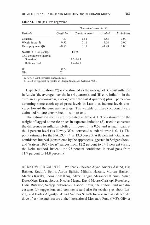
Olivier J. Blanchard, Mark Griffiths, and Bertrand Gruss 367
Expected inflation (p et ) is constructed as the average of: (i) past inflation
in Latvia (the average over the last 4 quarters); and (ii) core inflation in the euro area (year-on-year, average over the last 4 quarters) plus 1 percent—assuming some catch-up of price levels in Latvia as income levels con-verge toward the euro area average. The weights of these components are estimated but are constrained to sum to one.
The estimation results are presented in table A.1. The estimate for the weight of lagged domestic prices in expected inflation (d), used to construct the difference in inflation plotted in figure 17, is 0.57 and is significant at the 1 percent level (its Newey-West corrected standard error is 0.11). The point estimate for the NAIRU (u*) is 13.3 percent. A 95 percent “Gaussian” confidence interval (constructed by the approach suggested in Staiger, Stock, and Watson 1996) for u* ranges from 12.2 percent to 14.3 percent (using the Delta method, instead, the 95 percent confidence interval goes from 11.7 percent to 14.8 percent).
ACKNOWLEDGMENTS We thank Shekhar Aiyar, Anders Åslund, Bas Bakker, Rudolfs Bems, Aaron Eglitis, Mihails Hazans, Morten Hansen, Martins Kazaks, Joong Shik Kang, Alvar Kangur, Alexander Klemm, Ayhan Kose, Olegs Krasnopjorovs, Nicolas Magud, David Moore, Christoph Rosenberg, Uldis Rutkaste, Sergejs Saksonovs, Gabriel Srour, the editors, and our dis-cussants for suggestions and comments (and also for teaching us about Lat-via), and Bartek Augustyniak and Andreas Schaab for research assistance. All three of us (the authors) are at the International Monetary Fund (IMF). Olivier
Table A1. Phillips curve regression
Dependent variable: pt
Variable Coefficient Standard errora t-statistic Probability
Constant 7.30 1.51 4.83 0.00Weight in p e
t (d) 0.57 0.11 5.04 0.00Unemployment (b) -0.55 0.11 -4.98 0.00
NAIRU (- Constant/b) 13.2695% confidence interval Gaussianb 12.2–14.3 Delta method 11.7–14.8
R2 0.79Obs. 62
a. Newey-West corrected standard errors.b. Based on approach suggested in Staiger, Stock, and Watson (1996).
368 Brookings Papers on Economic Activity, fall 2013
Blanchard was the IMF's chief economist while the IMF- and EU-supported program was designed and implemented. Mark Griffiths was the IMF mission chief to Latvia from 2009 to 2012. Bertrand Gruss was a member of the IMF's Latvia mission team from 2012 to 2013.
References
Anosova, Daria, Konstantin Sonin, Alf Vanags, and Anna Zasova. 2013. “Structural or Cyclical? Unemployment in Latvia since the 2008–09 Financial Crisis.” CEPR Discussion Paper no. 9525. Washington, D.C.: Centre for Economic Policy Research.
Ashcraft, Adam. 2005. “Are Banks Really Special? New Evidence from the FDIC-Induced Failure of Healthy Banks.” American Economic Review 95: 1712–30.
———. 2006. “New Evidence on the Lending Channel.” Journal of Money, Credit and Banking 38, no. 3: 751–75.
Åslund, Anders, and Valdis Dombrovskis. 2011. “How Latvia Came Through the Financial Crisis.” Washington, D.C.: Peterson Institute for International Economics (May).
Bakker, Bas, and Christoph Klingen, editors. 2012. “How Emerging Europe Came Through the 2008/2009 Crisis.” Washington, D.C.: International Monetary Fund.
Bayoumi, Tam, and Ola Melander. 2008. “Credit Matters: Empirical Evidence on U.S. Macro-Financial Linkages.” Working Paper no. 08/169. Washington, D.C.: International Monetary Fund.
Bems, Rudolfs, and Julian Di Giovanni. 2013. “Sudden Stops and Expenditure Switching: Scanner Data Evidence from the 2008–09 Global Financial Crisis.” Mimeo. Washington, D.C.: International Monetary Fund.
Benkovskis, Konstantins. 2012. “Competitiveness of Latvia’s Exporters.” Working Paper no. 3/2012. Riga, Latvia: Bank of Latvia.
Bernanke, Ben, and Cara Lown. 1991. “The Credit Crunch.” Brookings Papers on Economic Activity 2: 205–47.
Berrospide, Jose, and Rochelle Edge. 2010. “The Effects of Bank Capital on Lending: What Do We Know, and What Does It Mean?” International Journal of Central Banking 6, no. 4: 5–54.
Blanchard, Olivier. 2007. “Adjustment within the Euro: The Difficult Case of Portugal.” Portuguese Economic Journal 6, no. 1 (April): 1–22.
———, Mitali Das, and Hamid Faruqee. 2010. “The Initial Impact of the Crisis on Emerging Market Countries.” Brookings Papers on Economic Activity, Fall.
Blanchard, Olivier, and Lawrence Katz. “Regional Evolutions.” 1992. Brookings Papers on Economic Activity, Spring: 1–75.
Boeri, Tito, and Pietro Garibaldi. 2006. “Are Labour Markets in the New Member States Sufficiently Flexible for EMU?” Journal of Banking and Finance 30, no. 5: 1393–1407.

Olivier J. Blanchard, Mark Griffiths, and Bertrand Gruss 369
Biggs, Michael, Thomas Mayer, and Andreas Pick. 2009. “Credit and Economic Recovery.” DNB Working Paper no. 218. Amsterdam: Netherlands Central Bank.
Claessens, Stijn, Ayhan Kose, and Marco Terrones. 2009. “What Happens during Recessions, Crunches and Busts?” Economic Policy 24: 653–700.
Calomiris, Charles, and Joseph Mason. 2003. “Consequences of Bank Distress during the Great Depression.” American Economic Review 93, no. 3: 937–47.
Central Bank of Ireland. 2011. “Compositional Effects in Recent Trends in Irish Unit Labour Costs.” (Box A on pages 22–24, prepared by Derry O’Brien.) Dublin.
Dao, Mai, David Furceri, and Prakash Loungani. 2013. “Regional Labor Adjustment in Currency Unions: Evidence from Europe and the United States.” Presentation at the 53rd European Regional Science Association (ERSA) Congress, Palermo, Italy, August 27–31. http://www.ersa.org/53rd-ersa-congress/.
Di Comite, Francesco, Gabriele Giudice, Radoslav Krastev, and Daniel Monteiro. 2012. “Fiscal Consolidation in the Midst of the Crisis.” EU Occasional Paper no. 120. http://ec.europa.eu/economy_finance/publications/occasional_paper/ 2012/op120_en.htm.
Driscoll, John. 2004. “Does Bank Lending Affect Output? Evidence from the U.S. States.” Journal of Monetary Economics 51, no. 3: 451–71.
Duchin, Ran, Oguzhan Ozbas, and Berk Sensoy. 2010. “Costly External Finance, Corporate Investment, and the Subprime Mortgage Credit Crisis.” Journal of Financial Economics 97: 418–35.
European Commission. 2005. “New and Updated Budgetary Sensitivities for the EU Budgetary Surveillance.” http://ec.europa.eu/economy_finance/economic_governance/sgp/pdf/budg_sensitivities_092005_v02_en.pdf.
———. 2012. “EU Balance of Payments Assistance for Latvia: Foundations of Success.” Occasional Paper no. 120 (November).
Greenlaw, David, Jan Hatzius, Anil Kashyap, and Hyun Song Shin. 2008. “Lever-aged Losses: Lessons from the Mortgage Market Meltdown.” U.S. Monetary Policy Forum Report No. 2, Rosenberg Institute, Brandeis International Business School and Initiative on Global Markets, and the University of Chicago Graduate School of Business.
Hazans, Mihails. 2007. “Coping with Growth and Emigration: Latvian Labor Market before and after EU Accession.” http://ssrn.com/abstract=971198.
———. 2011. “The Changing Face of Latvian Emigration, 2000–2010.” In Latvia—Human Development Report 2010/2011: National Identity, Mobility and Capa-bility, ed. by Brigita Zepa and Evija Klave. Riga: Advanced Social and Political Research Institute of the University of Latvia.
———. 2013. “Emigration from Latvia: Recent Trends and Economic Impact.” In Coping with Emigration: Policy Challenges and Responses in Baltic and East European Countries. Paris: OECD Publications.
———, and Kaia Phillips. 2010. “The Post-Enlargement Migration Experience in the Baltic Labor Markets.” In EU Labor Markets after Post-Enlargement
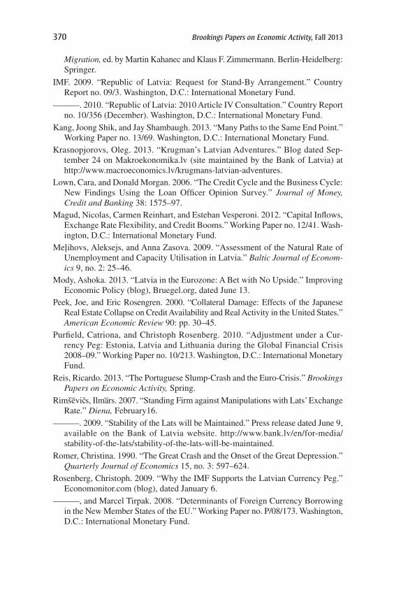
370 Brookings Papers on Economic Activity, fall 2013
Migration, ed. by Martin Kahanec and Klaus F. Zimmermann. Berlin-Heidelberg: Springer.
IMF. 2009. “Republic of Latvia: Request for Stand-By Arrangement.” Country Report no. 09/3. Washington, D.C.: International Monetary Fund.
———. 2010. “Republic of Latvia: 2010 Article IV Consultation.” Country Report no. 10/356 (December). Washington, D.C.: International Monetary Fund.
Kang, Joong Shik, and Jay Shambaugh. 2013. “Many Paths to the Same End Point.” Working Paper no. 13/69. Washington, D.C.: International Monetary Fund.
Krasnopjorovs, Oleg. 2013. “Krugman’s Latvian Adventures.” Blog dated Sep-tember 24 on Makroekonomika.lv (site maintained by the Bank of Latvia) at http://www.macroeconomics.lv/krugmans-latvian-adventures.
Lown, Cara, and Donald Morgan. 2006. “The Credit Cycle and the Business Cycle: New Findings Using the Loan Officer Opinion Survey.” Journal of Money, Credit and Banking 38: 1575–97.
Magud, Nicolas, Carmen Reinhart, and Esteban Vesperoni. 2012. “Capital Inflows, Exchange Rate Flexibility, and Credit Booms.” Working Paper no. 12/41. Wash-ington, D.C.: International Monetary Fund.
Melihovs, Aleksejs, and Anna Zasova. 2009. “Assessment of the Natural Rate of Unemployment and Capacity Utilisation in Latvia.” Baltic Journal of Econom-ics 9, no. 2: 25–46.
Mody, Ashoka. 2013. “Latvia in the Eurozone: A Bet with No Upside.” Improving Economic Policy (blog), Bruegel.org, dated June 13.
Peek, Joe, and Eric Rosengren. 2000. “Collateral Damage: Effects of the Japanese Real Estate Collapse on Credit Availability and Real Activity in the United States.” American Economic Review 90: pp. 30–45.
Purfield, Catriona, and Christoph Rosenberg. 2010. “Adjustment under a Cur-rency Peg: Estonia, Latvia and Lithuania during the Global Financial Crisis 2008–09.” Working Paper no. 10/213. Washington, D.C.: International Monetary Fund.
Reis, Ricardo. 2013. “The Portuguese Slump-Crash and the Euro-Crisis.” Brookings Papers on Economic Activity, Spring.
Rimse–vics, Ilma–rs. 2007. “Standing Firm against Manipulations with Lats’ Exchange Rate.” Diena, February16.
———. 2009. “Stability of the Lats will be Maintained.” Press release dated June 9, available on the Bank of Latvia website. http://www.bank.lv/en/for-media/stability-of-the-lats/stability-of-the-lats-will-be-maintained.
Romer, Christina. 1990. “The Great Crash and the Onset of the Great Depression.” Quarterly Journal of Economics 15, no. 3: 597–624.
Rosenberg, Christoph. 2009. “Why the IMF Supports the Latvian Currency Peg.” Economonitor.com (blog), dated January 6.
———, and Marcel Tirpak. 2008. “Determinants of Foreign Currency Borrowing in the New Member States of the EU.” Working Paper no. P/08/173. Washington, D.C.: International Monetary Fund.
Olivier J. Blanchard, Mark Griffiths, and Bertrand Gruss 371
Schadler, Susan, Ashoka Mody, Abdul Abiad, and Daniel Leigh. 2006. “Growth in the Central and Eastern European Countries of the European Union.” IMF Occasional Paper no. 252. Washington, D.C.: International Monetary Fund.
Shambaugh, Jay, and Joong Shik Kang. 2013. “The Evolution of Current Account Deficits in the Euro Area Periphery and the Baltics; Many Paths to the Same Endpoint.” Working Paper no. 13/169. Washington, D.C.: International Monetary Fund.
Staiger, Douglas, James H. Stock, and Mark W. Watson. 1996. “How Precise Are Estimates of the Natural Rate of Unemployment?” NBER Working Paper no. 5477. Cambridge, Mass.: National Bureau of Economic Research.
Vamvakidis, Athanasios. 2008. “Potential Growth Estimates in Emerging Europe Based on a Growth Model.” Box 8 in the EUR Regional Economic Outlook (April) Washington, D.C.: International Monetary Fund.
Vanags, Alf. 2013. “Latvia’s Exports: The Real ‘Success’ Story.” BICEPS Research Report. http://biceps.org/assets/docs/izpetes-zinojumi/Latvias_exports.
372
Comments and Discussion
COMMENT BYKRISTIN J. FORBES This paper by Olivier Blanchard, Mark Griffiths, and Bertrand Gruss offers an excellent and accessible description of the macroeconomic boom-and-bust cycle in Latvia from 2000 to 2012. It presents the key facts and data as well as is possible given the serious data challenges. It provides an unbiased analysis of different explanations for the country’s crisis and recovery, which is much appreciated, given how heated macroeconomists’ discussions on what actually happened in Latvia often have been.
Nonetheless, many readers of this volume may still be wondering, “Why Latvia?” Why should this distinguished group of authors and scholars dedicate an entire session to understanding the details of a small country that operated under a number of unique circumstances—especially during a period when many larger and more systemic economies were under severe economic distress? I will begin by answering this question and explaining why Latvia’s experience is worth closer investigation. I will then discuss three major insights from the paper—as well as the follow-up questions they inspire.
Why Study Latvia? Latvia provides one of the few examples of a country that did not follow the standard recommended response to a balance-of-payments crisis: allow a rapid devaluation of the currency in order to regain competitiveness and reduce the need for external financing. Instead, Latvia chose to maintain its currency peg and attempt an “internal devaluation,” that is, improve competitiveness through reductions in relative real wages. This process involved a period of sharply higher interest rates, a severe recession, and a fiscal contraction. In the past, other countries faced with similar balance-of-payments crises often hoped to adopt this strategy and avoid a currency devaluation, but most countries that embarked on this

commentS and diScuSSion 373
strategy soon abandoned it. Latvia is one of the few examples of a coun-try that persisted on this difficult path, avoided a currency devaluation, and accomplished an internal devaluation—much to the surprise of many economists and much faster than anyone expected.
In order to understand exactly how Latvia’s approach differs from the standard crisis response, it is useful to revisit a basic open-economy macro economics model. I will use what any graduate from MIT’s Ph.D. or M.B.A. program calls the BB-NN model (which is basically a variant of the Salter-Swan or dependent economy model). In this model, a country attempts to meet three constraints. First is the “external constraint,” represented in my figure 1 by the BB line, which requires that a country is in balance-of-payments equilibrium. Second is the “internal constraint,” represented by the NN line, which requires that a country has output at potential. Third is the rather nebulous “social peace” line, represented by the P line, which requires that real wages are above a level w in order to avoid protests and riots. The lines are graphed relative to output (Y) on the horizontal axis and
Source: Author.
B: devaluation option
C: Latvia2011 A: Latvia
2006
BB = external equilibrium
NN = internal equilibrium
P = social peace
Y = output
e/w = competitiveness
Figure 1. model of alternative crisis Responses
374 Brookings Papers on Economic Activity, Fall 2013
competitiveness (the ratio of the exchange rate to wages, or e/w) on the vertical axis.
In many examples, especially after a period of rapid growth financed by large capital inflows, a country finds itself in a situation like that shown in figure 1. The three lines in the model do not all intersect at any one point and the country is in the position marked by the dot A, labeled “Latvia 2006.” The country has output Y above potential and is to the right of the NN line. The country also has a large balance-of-payments deficit and is to the right of the BB line. Real wages are still high enough (helped by the overvalued exchange rate) that workers are “at peace” and not protesting, so the country still rests on the P line.
However, a country in such a situation is not able to stay at point A. At some point foreigners are no longer willing to finance the current account deficit and the country does not have sufficient reserves to maintain the overvalued exchange rate. The most common response to this balance-of-payments crisis is for a country to move to point B, the “Devaluation Option.” This involves a major and quick currency depreciation (e↑) and a sharp recession (Y↓). The country quickly moves to external balance, but the decline in real wages often causes protests and riots, the lack of social peace represented here by the country being located above the P line.
Latvia chose not to follow this standard response to a balance-of-payments crisis. Instead of devaluing its currency, it chose to keep e constant and instead move to a point such as C (labeled “Latvia 2011”). This involved a more gradual decline in real wages (w↓), which moved the country up on the graph, but not as far as if the currency had been devalued. It also involved a sharp increase in interest rates and a recession (Y↓), which may have moved the country more or less to the left on the graph relative to what would have occurred with a devaluation. (We will return to this ques-tion later.) The response also involved outward emigration, which shifted the NN line to the left.
The key point from figure 1 is that Latvia chose a different alternative than most other countries choose when responding to crises. To further illustrate how unique the Latvian response was, my figure 2 shows how countries responded to the period of global financial turmoil from 2007–11 (based on a sample of 85 countries). The graph basically shows the number of countries that chose to (i) sharply increase interest rates; (ii) allow large currency depreciations; (iii) intervene in foreign exchange markets using large amounts of reserves; and (iv) increase controls on capital outflows (details are available in Forbes and Klein 2013). The graph shows that the most popular response was to allow currency depreciations—which Latvia
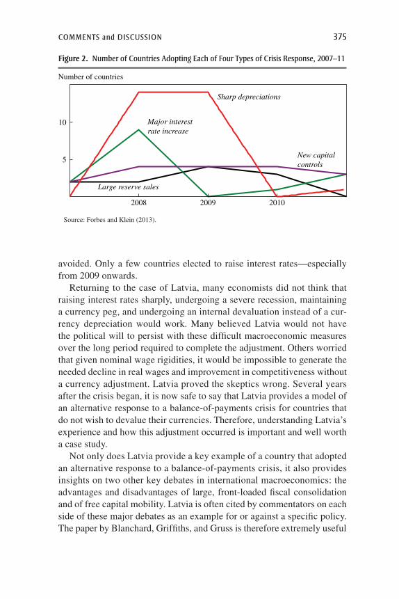
commentS and diScuSSion 375
avoided. Only a few countries elected to raise interest rates—especially from 2009 onwards.
Returning to the case of Latvia, many economists did not think that raising interest rates sharply, undergoing a severe recession, maintaining a currency peg, and undergoing an internal devaluation instead of a cur-rency depreciation would work. Many believed Latvia would not have the political will to persist with these difficult macroeconomic measures over the long period required to complete the adjustment. Others worried that given nominal wage rigidities, it would be impossible to generate the needed decline in real wages and improvement in competitiveness without a currency adjustment. Latvia proved the skeptics wrong. Several years after the crisis began, it is now safe to say that Latvia provides a model of an alternative response to a balance-of-payments crisis for countries that do not wish to devalue their currencies. Therefore, understanding Latvia’s experience and how this adjustment occurred is important and well worth a case study.
Not only does Latvia provide a key example of a country that adopted an alternative response to a balance-of-payments crisis, it also provides insights on two other key debates in international macroeconomics: the advantages and disadvantages of large, front-loaded fiscal consolidation and of free capital mobility. Latvia is often cited by commentators on each side of these major debates as an example for or against a specific policy. The paper by Blanchard, Griffiths, and Gruss is therefore extremely useful
Source: Forbes and Klein (2013).
5
10
2008 2009 2010
Large reserve sales
Sharp depreciations
Major interestrate increase
New capitalcontrols
Number of countries
Figure 2. number of countries adopting each of Four types of crisis Response, 2007–11
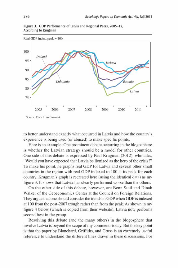
376 Brookings Papers on Economic Activity, Fall 2013
to better understand exactly what occurred in Latvia and how the country’s experience is being used (or abused) to make specific points.
Here is an example. One prominent debate occurring in the blogosphere is whether the Latvian strategy should be a model for other countries. One side of this debate is expressed by Paul Krugman (2012), who asks, “Would you have expected that Latvia be lionized as the hero of the crisis?” To make his point, he graphs real GDP for Latvia and several other small countries in the region with real GDP indexed to 100 at its peak for each country. Krugman’s graph is recreated here (using the identical data) as my figure 3. It shows that Latvia has clearly performed worse than the others.
On the other side of this debate, however, are Benn Steil and Dinah Walker of the Geoeconomics Center at the Council on Foreign Relations. They argue that one should consider the trends in GDP when GDP is indexed at 100 from the post-2007 trough rather than from the peak. As shown in my figure 4 below (which is copied from their website), Latvia now performs second best in the group.
Resolving this debate (and the many others) in the blogosphere that involve Latvia is beyond the scope of my comments today. But the key point is that the paper by Blanchard, Griffiths, and Gruss is an extremely useful reference to understand the different lines drawn in these discussions. For
Source: Data from Eurostat.
75
2005 2006 2007 2008 2009 2010 2011
80
85
90
95
100
Estonia
Ireland
Latvia
Lithuania
Iceland
Real GDP index, peak = 100
Figure 3. GdP Performance of Latvia and Regional Peers, 2005–12, according to Krugman
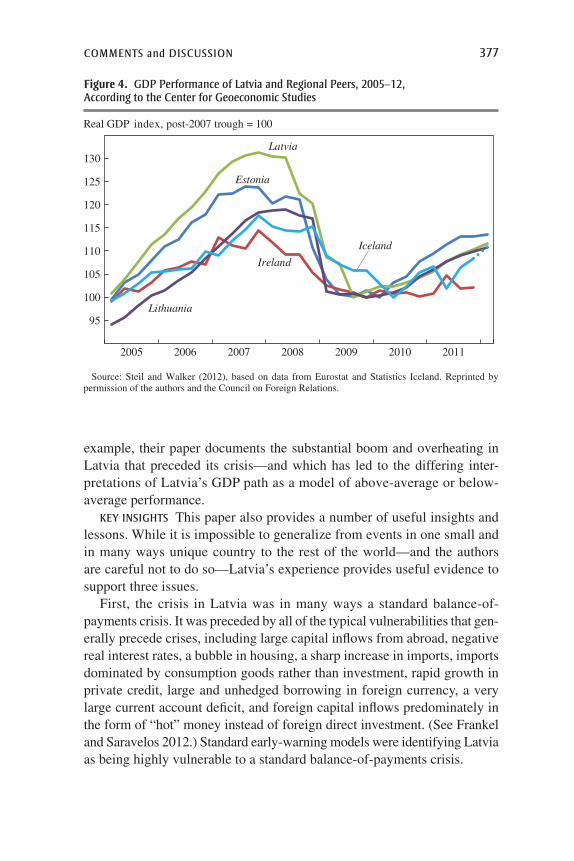
commentS and diScuSSion 377
example, their paper documents the substantial boom and overheating in Latvia that preceded its crisis—and which has led to the differing inter-pretations of Latvia’s GDP path as a model of above-average or below-average performance.
Key inSiGhtS This paper also provides a number of useful insights and lessons. While it is impossible to generalize from events in one small and in many ways unique country to the rest of the world—and the authors are careful not to do so—Latvia’s experience provides useful evidence to support three issues.
First, the crisis in Latvia was in many ways a standard balance-of- payments crisis. It was preceded by all of the typical vulnerabilities that gen-erally precede crises, including large capital inflows from abroad, negative real interest rates, a bubble in housing, a sharp increase in imports, imports dominated by consumption goods rather than investment, rapid growth in private credit, large and unhedged borrowing in foreign currency, a very large current account deficit, and foreign capital inflows predominately in the form of “hot” money instead of foreign direct investment. (See Frankel and Saravelos 2012.) Standard early-warning models were identifying Latvia as being highly vulnerable to a standard balance-of-payments crisis.
Source: Steil and Walker (2012), based on data from Eurostat and Statistics Iceland. Reprinted by permission of the authors and the Council on Foreign Relations.
95
2005 2006 2007 2008 2009 2010 2011
100
105
110
115
120
125
130
Estonia
Ireland
Latvia
Lithuania
Iceland
Real GDP index, post-2007 trough = 100
Figure 4. GdP Performance of Latvia and Regional Peers, 2005–12, according to the center for Geoeconomic Studies

378 Brookings Papers on Economic Activity, Fall 2013
Despite all the warning lights blinking bright red, the government was unable to prevent the economy from overheating and avoid a severe crisis. Several steps were taken to reduce credit growth, but these were too little, too late. This example suggests that even when a crisis is rela-tively easy to identify in advance, it is still extremely difficult for poli-cymakers to take preventive measures in a timely fashion. Is there a way to develop more automatic stabilizers to prevent crises if policymakers cannot act in time due to political or other constraints? Unfortunately, the evidence in the paper further indicates that any type of automatic stabilizers would be difficult to construct. For example, figure 5 in the paper shows the real-time, cyclically adjusted fiscal balance in Latvia and how this number was substantially revised over time. This challenge to access accurate information on key statistics in a timely fashion high-lights the challenge in preventing bubbles and crises in advance, even through automatic adjustment.
Second, the paper highlights the importance of quickly adjusting com-petitiveness. A key factor in Latvia’s ability to persist with its alternative strategy was its surprisingly rapid internal devaluation. This appears to have occurred due to a combination of productivity increases, layoffs, and emigration. Its success, however, raises even more questions on exactly how it was accomplished and if the experience could be replicated. For example, how important was Latvia’s small size to its ability to boost exports as part of its recovery? Does this experience suggest that labor market flexibility (firing) and mobility (emigration) are the key criteria to regain competitiveness with a fixed currency? If so, should countries hoping to share a currency (such as the euro) focus on these criteria rather than sharing fiscal risks (which is often included equally with labor market flexibility and mobility as a key criterion for an optimal currency area)? What are the long-term repercussions of this type of internal devaluation— especially if it involves policies such as the emigration of skilled workers?
Perhaps the most important question raised by Latvia’s example con-cerns the size of the contraction. If a country chooses to respond to a balance-of-payments crisis through an internal devaluation instead of a currency devaluation, will this generate a larger or smaller recession? Returning to my figure 1, will the country’s leftward movement (decline in Y ) from point A to point B be greater or less than its movement to point C? It is impossible to know the counterfactual, especially given the global turmoil that immediately followed Latvia’s bust, but better understanding why the contraction may have been less (or greater) under Latvia’s crisis-response strategy would be a useful addition to the paper.
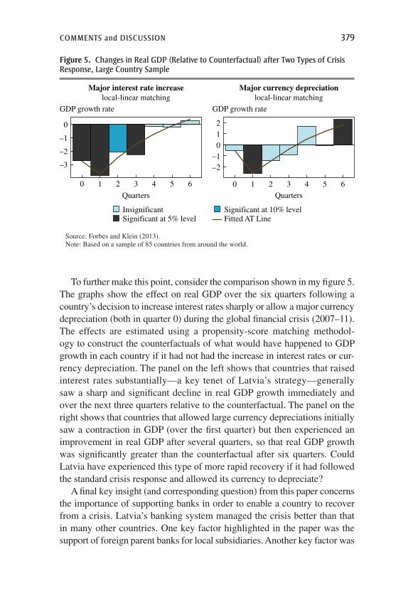
commentS and diScuSSion 379
To further make this point, consider the comparison shown in my figure 5. The graphs show the effect on real GDP over the six quarters following a country’s decision to increase interest rates sharply or allow a major currency depreciation (both in quarter 0) during the global financial crisis (2007–11). The effects are estimated using a propensity-score matching methodol-ogy to construct the counterfactuals of what would have happened to GDP growth in each country if it had not had the increase in interest rates or cur-rency depreciation. The panel on the left shows that countries that raised interest rates substantially—a key tenet of Latvia’s strategy—generally saw a sharp and significant decline in real GDP growth immediately and over the next three quarters relative to the counterfactual. The panel on the right shows that countries that allowed large currency depreciations initially saw a contraction in GDP (over the first quarter) but then experienced an improvement in real GDP after several quarters, so that real GDP growth was significantly greater than the counterfactual after six quarters. Could Latvia have experienced this type of more rapid recovery if it had followed the standard crisis response and allowed its currency to depreciate?
A final key insight (and corresponding question) from this paper concerns the importance of supporting banks in order to enable a country to recover from a crisis. Latvia’s banking system managed the crisis better than that in many other countries. One key factor highlighted in the paper was the support of foreign parent banks for local subsidiaries. Another key factor was
Source: Forbes and Klein (2013).Note: Based on a sample of 85 countries from around the world.
–3
–2
–1
0
GDP growth rate GDP growth rate
0 1 2 3 4 5 6
Quarters
Insignificant Significant at 10% levelSignificant at 5% level Fitted AT Line
Major interest rate increaselocal-linear matching
Quarters
Major currency depreciationlocal-linear matching
–2–1012
0 1 2 3 4 5 6
Figure 5. changes in Real GdP (Relative to counterfactual) after two types of crisis Response, Large country Sample
380 Brookings Papers on Economic Activity, Fall 2013
that because the currency did not depreciate, banks were not faced with as many bankruptcies and the corresponding increase in nonperforming loans, which generally follow when companies and consumers have unhedged liabilities (even if the banks had directly hedged their assets and liabilities against currency risk). Moreover, although one major domestic bank in Latvia required sovereign support, this did not create the large fiscal burden that occurred in other countries, such as Ireland.
The relative success in stabilizing Latvia’s banking system was undoubt-edly a key component of the country’s overall recovery. But returning to the question of why the Latvian experience is worth closer investigation—how did Latvia’s decision not to devalue influence the recovery of its banking system? If Latvia had chosen the standard currency-devaluation response, would this have generated a widespread increase in non-performing loans that would have caused more widespread banking collapses? Could this strat-egy have risked the support of foreign parents (or generated more financial support from them)? A closer look at how Latvia’s decision not to devalue its currency interacted with the financial system would add another useful dimension to the paper and help one to better understand one potential benefit of this alternative crisis response.
To conclude, this paper is an excellent case study of what happened in Latvia over the 2000s. It illustrates a textbook case of the standard buildup to a balance-of-payments crisis and provides a rare example of a nonstandard response. The case study is a superb example for teaching concepts and for better understanding one of the options that countries consider when faced with a balance-of-payments crisis. Latvia’s experience provides use-ful insights into several major questions, such as why it is so difficult for policymakers to prick bubbles, how a country can regain competiveness with a fixed exchange rate, and the importance of a strong banking system. Each insight, however, generates more questions—especially the question of how Latvia’s example could be generalized to other countries. More case studies in this vein—of large and small countries alike—would be helpful to better understand the policy options countries face.
ReFeRenceS FoR the FoRbeS comment
Forbes, Kristin, and Michael Klein. 2013. “Pick Your Poison: The Choices and Consequences of Policy Responses to Crises.” Working Paper no. 5062-13. Cambridge, Mass.: MIT Sloan School of Management.
Frankel, Jeffrey, and George Saravelos. 2012. “Can Leading Indicators Assess Country Vulnerability? Evidence from the 2008–09 Global Financial Crisis.” Journal of International Economics 87 (2): 216–31.
commentS and diScuSSion 381
Krugman, Paul. 2012. “Peripheral Performance.” Conscience of a Liberal (blog), New York Times, June 14. http://krugman.blogs.nytimes.com/2012/06/14/peripheral-performance/.
Steil, Benn, and Dinah Walker. 2012. “Iceland’s Post-Crisis ‘Miracle’ Revisited.” Geo-Graphics (blog), July 2, Center for Geoeconomic Studies, Council on Foreign Relations (http://blogs.cfr.org/geographics/2012/07/02/postcrisis/).
COMMENT BYPAUL KRUGMAN Olivier Blanchard, Mark Griffiths, and Bertrand Gruss have given us a terrific paper on Latvia, welcome for its tone as well as its content. Latvia has become a symbol in the fiscal policy wars, with austerity advocates elevating it to iconic status; the temptation must have been strong either to validate that elevation or to turn the paper into an exercise in debunkery. Instead, the authors give us a detailed, balanced account—one that highlights just how odd, how inconsistent with the orthodoxies of either side, the Latvian experience seems to be.
Let me dive right into the two big issues the paper raises: the puzzle of Latvia’s output gap and the puzzle of its internal devaluation.
Here is what is known: Latvia suffered a huge, Depression-level economic contraction after 2007, followed eventually by a fast but as yet incomplete bounce-back—which the latest data suggest may be slowing—that has left unemployment much higher than it was pre-crisis. Actually, Latvia’s numbers from 2007 to 2013 look fairly similar to those for the United States from 1929 to 1935. Today, everyone considers America in 1935 to have been still in the depths of the Great Depression, so if one looks at Latvia through the same lens the country doesn’t look very good—better than Greece, perhaps, but not good.
However, the Latvian authorities tell a very different story, and the authors basically agree. The authors argue that 2007 is a misleading base, that the Latvian economy on the eve of the crisis was wildly overheated, with a positive output gap of something like 12 percent. And they cor-respondingly conclude that Latvia has in large part already recovered more or less fully. They do not arrive at this conclusion lightly. But I do think it is worth asking how plausible it is.
First of all, on a conceptual level, how does an economy get to operate far above capacity? We all understand operating below capacity: producers may fail to produce as much as they would prefer to if there is not enough demand for their products. But how does excess demand induce producers to produce more than they want to? New Keynesian models actually have
382 Brookings Papers on Economic Activity, Fall 2013
something of an answer: The economy is monopolistically competitive, so producers in general charge prices above marginal cost and are hence willing to produce more given the demand. But there has to be some limit to this margin. Is 12 percent really plausible?
Second, how often does one see the kind of huge positive gap that is being posited for Latvia? Or to ask a question that can actually be answered, how often does the IMF estimate output gaps that big? I have gone through the IMF’s World Economic Outlook Database, looking at all advanced countries since 1980, to identify double-digit positive output gaps. Here’s the full list:
Estonia 2007Greece 2007Italy 1980Luxembourg 1991
I have no idea what was going on in Italy in 1980 or in Luxembourg in 1991. I doubt that anyone believes that Greece was operating at 10 percent above capacity in 2007. Surely what is showing up here is a problem with the methods the IMF uses to estimate potential output. Basically, the Fund uses a weighted average of actual output over time. This automatically interprets any sustained decline in actual output as a decline in potential, and it causes that re-estimate to propagate backward through time. So the catastrophe in Greece ends up leading to the basically silly conclusion that there was a hugely overheated economy there before the crisis.
In addition, whatever is going on in Estonia presumably bears some relationship to what is going on in Latvia. The point is, if Latvia really was as hugely over capacity as the authors claim—and to be fair, they do not use the filtering method but instead make a careful assessment of unemployment and inflation—it represents a more or less unique case.
And arguing that Latvia was vastly over capacity in 2007 has another, perhaps surprising implication: It makes much of the debate over both austerity and internal devaluation moot.
On austerity: If one were really looking at an economy with a double-digit inflationary output gap, even the most ultra-Keynesian Keynesian would call for fiscal austerity. Once one grants the output gap inter-pretation, the fiscal policy debate evaporates. To an important degree, the internal-versus-external devaluation debate evaporates as well.
My figure 1 plots Latvian growth, at an annual rate, versus the one-year change in the current account balance as a percentage of GDP. There was a strong relationship both before and after the crisis, but if anything it was

commentS and diScuSSion 383
stronger before the crisis. Given the slump in Latvian output after 2007, one should have expected a huge external adjustment from that fact alone. Maybe Latvia did not need a devaluation of any kind, external or internal. Maybe it was not overvalued, just overheated.
That said, the authors also provide evidence of a substantial internal devaluation, at least as measured by unit labor costs. Oddly, however, almost none of this comes by means of lower wages: wages in manufactur-ing have been every bit as flat as those of us who warned about downward nominal wage rigidity would have predicted. Instead, what one sees is a rapid rise in productivity, which the authors suggest is the result of eliminating X-inefficiency.
However, there may also be an alternative interpretation. Latvia is a relatively poor European country playing catch-up, and it had rapid produc-tivity growth before as well as after the crisis. My figure 2 shows aggregate labor productivity from Eurostat. Maybe Latvia just had an impressive productivity trend owing to its particular position in the European system and simply returned to that trend after a brief setback.
How does that bear on the internal devaluation debate? If Latvia had very high productivity growth, for whatever reason, the serious thing advo-cates of currency flexibility worry about, namely the downward rigidity of nominal wages, was not a binding constraint.
Suppose, instead, this story: Latvia was a hugely, perhaps uniquely overheated economy that even a Keynesian would agree needed a lot of fiscal austerity, a country with very high rates of productivity growth making wage stickiness irrelevant. I am not sure I believe this story, but for those who do, what lessons does Latvia hold for other countries and for the eurozone in general?
Source: IMF, World Economic Outlook database.
–20
–10
0
10
20
–15 –10 –5 0 5 10
Change in current account
Growth in GDP
2000–20072008–2012
Figure 1. Growth and external adjustment, Latvia, during two Periods
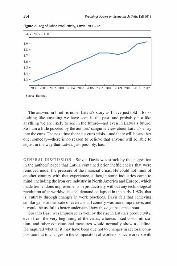
384 Brookings Papers on Economic Activity, Fall 2013
The answer, in brief, is none. Latvia’s story as I have just told it looks nothing like anything we have seen in the past, and probably not like anything we are likely to see in the future—not even in Latvia’s future. So I am a little puzzled by the authors’ sanguine view about Latvia’s entry into the euro. The next time there is a euro crisis—and there will be another one, someday—there is no reason to believe that anyone will be able to adjust in the way that Latvia, just possibly, has.
GENERAL DISCUSSION Steven Davis was struck by the suggestion in the authors’ paper that Latvia contained prior inefficiencies that were removed under the pressure of the financial crisis. He could not think of another country with that experience, although some industries came to mind, including the iron ore industry in North America and Europe, which made tremendous improvements in productivity without any technological revolution after worldwide steel demand collapsed in the early 1980s, that is, entirely through changes in work practices. Davis felt that achieving similar gains at the scale of even a small country was more impressive, and it would be useful to better understand how those gains came about.
Susanto Basu was impressed as well by the rise in Latvia’s productivity, even from the very beginning of the crisis, whereas fixed costs, utiliza-tion, and other conventional measures would normally show a decline. He inquired whether it may have been due not to changes in sectoral com-position but to changes in the composition of workers, since workers with
Source: Eurostat.
Index, 2005 = 100
4.3
4.4
4.5
4.6
4.7
4.8
4.9
2000 2001 2002 2003 2004 2005 2006 2007 2008 2009 2010 2011 2012
Figure 2. Log of Labor Productivity, Latvia, 2000–12
commentS and diScuSSion 385
lower productivity are normally the first ones to be fired. In a deep down-turn, only the most productive workers would be retained, so perhaps labor productivity in Latvia wasn’t growing as fast as it appeared to be and that wages were therefore falling much faster than they appeared to be. All of this would mean that internal devaluation was even more successful than one had thought.
John Haltiwanger asked whether compositional effects within sectors were the determinative factor in productivity increases, given that the authors showed sectoral composition was not determinative. Substantial productivity increases can be attained from such changing composition, particularly in countries undergoing reforms. Haltiwanger suggested that if Basu were correct about worker retention, in Latvia such within-firm productivity increases should be evident. Alternatively, Latvia’s productivity growth could have stemmed from the reallocation of labor, as has happened in countries undergoing market reform, including China, India, and much of eastern Europe. What remained puzzling about Latvia was how quickly all of this happened.
David Romer pointed out that no internal devaluation (in the sense of a fall in prices relative to those of other countries) appeared to have actually happened in Latvia, so the question remains, What caused the export boom? He suggested three possible answers. One, implicit in Paul Krugman’s comment, is that there might have been no export boom in the first place, only a natural response to what was happening to output and the cooling off of the economy. A second answer, which Olivier Blanchard had implicitly suggested in his presentation, was that because Latvian producers were earning such enormous profit margins they had incentives to drum up new customers. This answer appears to require that they were able to do so without much labor input, since productivity did not fall. It would also imply that Latvia’s producers did not take advantage of that situation until their labor costs went down. Romer observed that the paper did not present evi-dence in favor of these implications of this explanation. A third explanation might simply be that “they got lucky,” that is, that the export boom had nothing to do with the fall in unit labor cost, since that did not translate into lower prices.
Caroline Hoxby suggested that Latvia’s export boom might be explained as stemming from the reallocation of labor between firms, returning to a possibility Haltiwanger had raised. She wondered whether the firms that gained a lot of the labor market share within their industry were the very ones that were already good exporters. Firms’ propensity to export varies widely even in the same industry, so efficient firms could have taken business from
386 Brookings Papers on Economic Activity, Fall 2013
inefficient ones. It also seemed to Hoxby that the productivity gains were indeed real, since the workers who relocated must have been hired to do work in Europe that was at least as productive as what they were previously doing in Latvia. She would like to know whether those gains would have happened in Latvia without the sharpness of the fiscal consolidation and the government’s willingness to stick to the peg. The most important question for her was whether there was a causal link between those decisions and productivity or whether it was only a case of coincidence.
Justin Wolfers took issue with Hoxby’s suggestion that the productivity gains were real, noting that growth by 50 percentage points in four years would normally suggest something was wrong with the data. The simplest way to test this would be to ask what the natural implications in the economy would be following such a sharp productivity boom and then look for them. Above all, one would expect to see a change in prices, yet in Latvia no major price changes were observed. This leaves open the question of what has actually been going on in the country.
Richard Cooper agreed with Romer that the authors’ data showed no evidence of an internal devaluation in Latvia, and agreed with several others as well that the biggest puzzle was the rise in productivity. Internal devaluations, he added, can indeed be relevant to export booms, as in the case of Germany, which stimulated exports in 2007 by reducing labor taxes and raising the VAT, but such an internal devaluation did not occur in Latvia.
Benjamin Friedman raised the issue of Latvia’s massive emigration. Half a decade in which 1.0 to 1.5 percent of the country’s population emigrated each year would be comparable to 20 million people exiting the United States during the same period. Should we emphasize the fact that this population movement was mostly within Europe, and therefore think of it as similar to a migration of workers from Michigan to Arizona, that is, a natural movement of labor that did not disturb the country as a whole? Or should we instead think of it as similar to labor leaving the United States altogether? In the first case, unemployment would be much less of a problem if workers could relocate so easily, although as a “solution” that would risk igniting serious social unrest. Friedman also thought the matter raises the question of what determines whether somebody who has lost a job decides to exit the country. Krugman had suggested that emigration is a big part of the Latvia story, and not as a problem, because Latvia is actually more like Michigan in the analogy. If that is correct, the lesson may be that one cannot apply the Latvian experience to a “normal” country.

commentS and diScuSSion 387
Paul Krugman added that in the European context, issues of emigration require one to consider the lack of fiscal integration there. By contrast, when people leave Michigan for Arizona, this does not create a problem of who is going to pay their social security and Medicare benefits. When Portuguese leave Portugal, however, there is a very real concern over who will be left to pay for the benefits needed by those people who remain behind in the old country.
Robert Gordon was struck by the authors’ finding that Latvian pro-ductivity had risen for 11 years by about 8 percent per year, in striking contrast with the euro zone, where it barely rose at all between 1995 and 2011. As an emerging country rapidly catching up to western methods of production, Latvia had the latitude to make radical changes in its unit labor cost, something that the problem countries of Europe could not do. Italy has experienced zero productivity growth for the last decade, and the potential for cutting unit labor cost there seemed to Gordon vastly differ-ent than in Latvia. Even in the United States, although productivity briefly boomed during the recession, it has almost completely stagnated since.
Valerie Ramey was most surprised by the authors’ finding that the natural rate of unemployment in Latvia is around 12 percent, an exceptionally high rate for a country with a low minimum wage, weak unions, and limited unemployment insurance and employment protection. To her, this strained credibility. Was there a gross mismeasurement of the price level and hence inflation, or a gross mismeasurement of the unemployment rate? Or did this show that something is fundamentally wrong about the Phillips curve itself?
Gregory Mankiw too wondered whether Latvian measures were to be trusted at face value. He questioned whether the measures of unemploy-ment there are reliable, for example whether cultural differences may cause people to answer surveys about looking for work differently than they do elsewhere. The fuzziness of the concepts of unemployment and labor force could also be contributing to the surprising findings.
Christopher Carroll expanded on a point made by Gordon regarding Latvia’s uniqueness, specifically that its economy had been growing so quickly for a long time leading up to the crisis. If the macroeconomic find-ings on the importance of habit formation published in the last dozen years are correct, it will be much easier for Latvia to readjust back downward to where the country was three years ago than it will be for Portugal to readjust to below where it was three years ago. He added that many of the stories about the relative ease or difficulty countries have had in adjusting strongly suggest that habits might matter for governments as much as they do for people.

388 Brookings Papers on Economic Activity, Fall 2013
Olivier Blanchard responded to the various points raised. Clearly a cen-tral question is what stands behind high productivity growth. Strong labor shedding, induced in part by the credit crunch, was surely a factor at the start. But now, many sectors have higher employment and higher output than before the crisis, so more than labor shedding is at work. Regarding composition effects, he noted that while there was no evidence of sectoral composition effects, there was some evidence of skill composition effects. At the same time, the proportion of unskilled workers in unemployment is higher than it was before the crisis. Regarding wage adjustments, he noted that while public sector wages were lowered by 20 percent, private sector wages dropped only slightly.
Blanchard had this to say regarding the comparison between internal and external devaluations: One might argue that an external devaluation would have decreased the pressure to achieve productivity improvements, and that it may have triggered sharp adverse balance sheet effects, in response to the sudden increase in the domestic value of foreign currency liabilities. As far as the small decrease in export prices and the behavior of exports, he noted that if exporters are price takers in foreign markets, and the effect of a decrease in unit labor costs shows up in profit margins rather than in prices, the increase in profit margins may lead new firms to enter the export market and existing firms to increase production. Given that Latvia is a small country and has a small market share, it may indeed be a price taker in most export markets, and this may be the explanation behind rapid export growth.
Finally, Blanchard very much agreed with Krugman that, in the context of sharp export growth before the crisis, the return to rapid export growth may not be that much of a surprise. Clearly, things would be and are very different in countries that stagnated before the crisis.