BOOK-TAX DIFFERENCES AND EARNINGS GROWTH

by

MARK JACKSON

A DISSERTATION

Presented to the Department of Accountingand the Graduate School of the University of Oregon

in partial fulfillment of the requirementsfor the degree of

Doctor of Philosophy

June 2009

11

University of Oregon Graduate School

Confirmation of Approval and Acceptance of Dissertation prepared by:

Mark Jackson

Title:

"Book-Tax Differences and Earnings Growth"

This dissertation has been accepted and approved in partial fulfillment of the requirements forthe Doctor of Philosophy degree in the Department of Accounting by:

David Guenther, Chairperson, AccountingSteven Matsunaga, Member, AccountingLinda Krull, Member, AccountingGlen Waddell, Outside Member, Economics

and Richard Linton, Vice President for Research and Graduate Studies/Dean of the GraduateSchool for the University of Oregon.

June 13,2009

Original approval signatures are on file with the Graduate School and the University of OregonLibraries.

in the Depmiment of Accounting

Mark Jackson

An Abstract of the Dissertation of

for the degree of

to be taken

111

Doctor of Philosophy

June 2009

Title: BOOK-TAX DIFFERENCES AND EARNINGS GROWTH

Approved:Dr. David Guenther

I examine the relation between book-tax differences (BTDs) and earnings growth.

Because financial accounting rules afford managers more flexibility and discretion in

repOliing than tax accounting rules, prior studies suggest that large differences between

book and taxable income indicate lower quality (or less persistent) earnings. Lev and

Nissim and Hanlon provide evidence that BTDs contain infonnation about future finn

performance, but the nature of the causality in this relation is not clear. While BTDs

could proxy for earnings quality, they may also reveal underlying economic events or

management's private information about future perfonnance or simply predict future

reversals in effective tax rates.

I divide total BTDs into their measurable components: temporary (defelTed taxes)

and non-temporary (pennanent differences and tax accruals), and test their relation with

the components of net income changes: pretax earnings changes and tax expense

changes. I hypothesize that the non-temporary component ofBTDs is negatively related

IV

to future changes in tax expense, whereas the temporary component ofBTDs is

negatively related to changes in future pretax eall1ings. I also examine the maintained

hypothesis that the lower earnings growth for large BTD finTIs is due to earnings

management. I use various proxies from prior literature to identify fin11s potentially

managing earnings and test whether the presence or absence of suspected earnings

management activity alters the relation between BTDs and earnings changes.

My results provide compelling evidence that pell11anent BTDs are related only to

future changes in tax expense, and temporary BTDs are related to changes in pretax

eall1ings. These results are robust to multiple sensitivity analyses, including a replication

of the sample and methodology of Lev and Nissim. The results also hold in the case of

fill11s not suspected of eall1ings management. In fact, I find only limited evidence that the

results are stronger in the presence of earnings management. Overall, my study suggests

that it is only the temporary component of BTDs that is related to future firm

performance, with non-temporary differences being related to future tax expense changes,

and that these results are primarily due to underlying economic factors, not eall1ings

management.

CURRICULUM VITAE

NAME OF AUTHOR: Mark Jackson

PLACE OF BIRTH: Torrance, California

DATE OF BIRTH: December 29,1963

GRADUATE AND UNDERGRADUATE SCHOOLS ATTENDED:

University of Oregon, EugeneUniversity of Texas, El Paso

DEGREES AWARDED:

Doctor of Philosophy, Accounting, June 2009, University of OregonBachelor of Science, Accounting, May 2005, University of Texas, El Paso

AREAS OF SPECIAL INTEREST:

The interaction of financial and tax accounting systemsEarnings management and firm value

PROFESSIONAL EXPERIENCE:

Graduate teaching fellow, University of Oregon, 2005-presentOwner/Manager, Jackson Bookkeeping and Tax Preparation, 1998-present

GRANTS, AWARDS AND HONORS:

Accounting Circle at Lundquist College of Business Summer Fellowship,2007

Beta Gamma Sigma, business honor fraternity, admitted 2005Summa Cum Laude, University of Texas, El Paso, 2005

v

ACKNOWLEDGMENTS

I am thankful for the guidance ofmy dissertation committee: Dave Guenther

(chair), Linda Krull, Steve Matsunaga, and Glen Waddell. This paper has also benefited

from discussions with Lisa Eiler, Josh Filzen, Isho Tama-Sweet, Dave Weber, and

workshop participants at Central Missouri University, Eastern Michigan University,

Louisiana State University, Texas Tech University, University of Oregon, University of

Nevada, Reno, and University ofNorth Texas.

VI

VB

TABLE OF CONTENTS

Chapter Page

I. INTRODUCTION 1

II. RELATED RESEARCH......................................................................................... 7

Temporary Differences 7

Total Differences 8

III. HYPOTHESIS DEVELOPMENT......................................................................... 11

Tax Accruals.......................................................................................................... 13

Permanent Differences 16

Telnporary Differences 17

IV. RESEARCH DESIGN........................................................................................... 22

V. SAMPLE AND SUMMARY STATISTICS 30

Sample Selection.................................................................................................... 30

Summary Statistics............... 31

VI. EMPIRICAL RESULTS 34

The Association between Book-Tax Differences and Earnings Changes 34

Impact of Earnings Management on Association between Book-Tax

Differences and Earnings Growth.................................................................... 37

VII. ROBUSTNESS AND SENSITIVITY TESTS..................................................... 45

Reconciliation with Lev and Nissim (2004) 45

V111

Chapter Page

Firm Fixed Effects 51

Negative Income and Tax Expense........................................................................ 53

Ranked Regressions and Measurement of Cash from Operations 53

Absolute Values 55

Foreign Operations................................................................................................. 58

Earnings Managelnent 58

VIII. CONCLUSION 61

BIBLIOGRAPHy..... 63

IX

LIST OF FIGURES

Figure Page

1. Five-Year Growth in Net Income and its Components for Portfolios of FirmsSorted by BTD and Cash Flow Measures........................................................ 47

LIST OF TABLES

Table Page

1. Example of Relation between Book-Tax Differenceand Future Performance................................................................................... 14

2. Means of Effective Tax Rates (ETR) Across Ranks ofBTDFor Five Years Prior to and After BTD Ranking............................................. 15

3. Comparison of Variable Means Across Extremes in BTDs 32

4. Correlation Matrix 33

5. Regressions of Future Earnings Changes on BTD Measures and OtherIndicators of Growth 35

6. Examining Effect of EM on BTD Coefficients: Small Earnings Changes............ 39

7. Examining Effect of EM on BTD Coefficients: Narrowly Avoiding a Loss ........ 40

8. Examining Effect of EM on BTD Coefficients: Analysts' Forecasts.................... 42

9. Examining Effect of EM on BTD Coefficients: Discretionary Accruals 43

10. Regressions of Future Earnings Changes on BTD Measures and OtherIndicators of Growth: Lev and Nissim (2004) Methodology................................ 49

11. Regressions of Future Earnings Changes on BTD Measures and OtherIndicators of Growth: Firm Fixed Effects.............................................................. 52

12. Regressions of Future Earnings Changes on BTD Measures and OtherIndicators of Growth: Including Firms with Negative Income and Tax................ 54

13. Regressions of Future Earnings Changes on BTD Measures and OtherIndicators of Growth: Ranked Regressions 56

14. Regressions of Future Earnings Changes on BTD Measures and OtherIndicators of Growth: Using Absolute Values of BTDs 57

15. Examining Effect of Foreign Operations on BTD Coefficients 59

x

I

CHAPTER I

INTRODUCTION

In this paper I examine the relation between book-tax differences (BTDs) and

earnings growth. Prior literature (Lev and Nissim, 2004; Hanlon, 2005) provides

evidence that BTDs contain information about future firm performance, but the nature of

the causality in this relation is not clear. Lev and Nissim (2004) suggest that BTDs

capture earnings management activity, or that tax accounting better captures 'core'

earnings. As tax accounting is more closely associated with current cash flows, the

magnitude of BTDs could capture the extent to which book income ventures away from

its 'permanent' levels. However, to the extent that BTDs capture underlying economic

items that are transitory in nature (such as a goodwill write-off or restructuring charge),

any relation between BTDs and earnings growth could simply be related to these events.

It is also possible that the book-tax difference predicts future variation in effective tax

rates (and therefore tax expense).

To examine these issues, I study the effect of the temporary and permanent

components of BTDs on future changes in both pretax earnings and tax expense. If BTDs

(or one of its components) contains infonnation about the future economic performance

of the firm, I expect to find a relation between this measure and future changes in pretax

earnings. However, ifBTDs (or its components) contains information about future

effective tax rates, then I expect to find a relation between this measure and future

changes in tax expense. In addition, prior literature is unsettled as to which measure of

BTD better proxies for earnings quality, as Lev and Nissim (2004) and Hanlon (2005)

find conflicting results using different BTD measures. By examining the effect of

different components ofBTDs on earnings growth, my research design reconciles the

conflicting findings of previous research, and provides guidance for future work

examining the relation between BTDs and future firm performance. Finally, I examine

the relation between BTDs and earnings growth in the presence and absence of earnings

management. If the BTD/earnings growth relation holds even in the absence of earnings

management, this would suggest that any relation between BTDs and earnings growth is

due at least in part to mechanical and economic factors rather than opportunistic

behavior. Understanding the relation between BTDs and future earnings changes is

important because it provides evidence on the usefulness of taxable income in

determining firm value.

Book-tax differences arise when different accounting systems are applied to the

same set of underlying economic events. Recent research has attempted to detennine

whether these differences are informative about a firm's earnings characteristics and

future performance. Lev and Nissim (2004) suggest that BTDs are related to growth

because they reflect earnings management activities that are not persistent or capture the

extent to which book earnings deviate from their permanent level. They predict and find

that BTDs are positively related to future earnings growth. 1 However, because they

2

I It should be noted that although Lev and Nissim (2004) use the tax to book ratio to capture theimpact of total BTDs on earnings growth, their inclusion of the temporary component, deferred taxes,in their tests implies that the coefficient on the tax to book ratio is really capturing the impact of thepermanent component of BTDs on earnings growth. I discuss this issue and my approach in theresearch design section.

3

measure growth as changes in net income, the growth they document could be related to

changes in underlying pretax earnings, or to changes in future income tax expense. To

distinguish these two effects, I separate growth in net income into its two components,

pretax earnings and tax expense, and separate total BTDs into its two components,

permanent and temporary differences. I then examine the effect of the two components of

BTDs on the growth of each income component. I find that permanent BTDs are not

positively related to growth in pretax earnings, but negatively related to changes in tax

expense, suggesting that permanent BTDs are more relevant in predicting future effective

tax rates than future core earnings growth.

Lev and Nissim (2004) also examine the relation between temporary BTDs

(deferred taxes) and earnings growth, and find no evidence of a relation. In contrast,

Hanlon (2005) finds evidence of lower earnings persistence for firms with large

temporary BTDs. In an effort to reconcile these conflicting results, I examine the relation

between temporary BTDs and the two components of earnings growth, pretax earnings

and tax expense. Consistent with Hanlon (2005), I find that growth in pretax income is

negatively related to temporary BTDs. My findings, that changes in future tax expense is

negatively related to non-temporary BTDs (permanent differences and tax accruals),

while growth in pretax income is negatively related to temporary BTDs, provides

evidence about which BTD measure is most appropriate in a given research setting, such

4

as investigations into how market participants use the BTD information in their decision

k· 2ma mg processes.

A common theme in the BTD literature, and in the public press, is the concept

that BTDs proxy for earnings quality or represents earnings management. For example,

Rep. Lloyd Doggett (D-Tex.) referred to "a corporate culture of creative accounting and

reporting abuses" when he introduced legislation requiring companies to disclose and

explain the gap between book and taxable income (Weisman 2002, AOl). Phillips,

Pincus, and Rego (2003) present evidence that suggests that large BTDs are associated

with various measures of earnings management. Hanlon and Krishnan (2006) interpret

evidence of higher audit fees for firms with large BTDs as evidence that auditors

associate large BTDs with increased risk of earnings management. On the other hand,

Tang (2007) and Dhaliwal, Huber, Lee, and Pincus (2008) argue that much of the BTD is

due to mechanical or economic differences, unrelated to opportunistic behavior. To better

understand the relation between earnings growth and BTDs, I control for various proxies

of earnings management. While the relation between growth and BTDs holds for films

with no indication of opportunistic behavior, I find only weak evidence that firm years

suspected of earnings management have a stronger growth/BTD relation, suggesting that

it is principally underlying economic events, and not earnings management, that is

responsible for the relation between earnings growth and book-tax differences.

2 Prior literature is unsettled as to the appropriate measure for BTDs. Phillips, Pincus, and Rego(2003) and Joos, Pratt, and Young (2000) focus on temporary differences, Weber (2008) andDhaliwal, Huber, Lee, and Pincus (2008) focus on total BTDs, while Hanlon and Krishnan (2006) useboth. See the following chapter for a discussion of these papers.

5

This research makes several contributions. First, while plior literature suggests

that BTDs are related to future earnings growth, it is not clear whether this growth is

related to future changes in core economic performance, future changes in tax expense, or

both. I provide evidence that growth in the two components of net income, pretax

earnings and tax expense, are related in different ways to BTDs. Second, I address the

unsettled question as to which BTD measure best predicts earnings growth. I find that

temporary differences predict growth in pretax earnings, while permanent differences

predict earnings growth related to changes in tax expense. These findings also help

reconcile the conflicting results of Lev and Nissim (2004) and Hanlon (2005) on the

relation between temporary BTDs and earnings growth/persistence. Third, this study

answers the call of Graham, Raedy, and Shackelford (2008) and Hanlon and Heitzman

(2009) for an examination ofthe components ofBTDs. Although Graham, Raedy, and

Shackelford (2008) ultimately desire a study that examines the specific accounts that

leads to BTDs and why they are informative, my study is a first step in at least breaking

BTDs into their temporary and permanent components, and understanding why and how

each component is informative. Hanlon and Heitzman (2009) specifically ask for an

examination of Lev and Nissim's (2004) results on non-temporary BTDs, indicating that

a better understanding of their results would progress the literature. Finally, I contribute

to the debate regarding book-tax conformity. Proponents of bridging the book-tax gap

assert that the gap exists due to opportunistic behavior, but my results suggest that the

relation between earnings growth and BTDs are more the result of underlying economic

events that are manifest in book-tax differences.

The remainder of the paper is organized as follows. The next Chapter highlights

related literature. Chapter III develops the hypotheses and Chapter IV discusses the

research design. Chapter V describes the sample employed in the empirical tests and

Chapter VI presents the results of those tests. Chapter VII presents robustness checks. I

provide concluding comments and avenues for future research in Chapter VIII.

6

7

CHAPTER II

RELATED RESEARCH

Recent research examines the association between BTDs and earnings quality.

Mills and Newberry (2001) find evidence consistent with firms increasing BTDs when

the nontax costs of conforming book to tax income outweigh the tax-related costs of non­

conformity. Public firms, those with high debt or facing financial distress, as well as

those near bonus plan thresholds or with specific earnings patterns were associated with

larger BTDs. Their measure of BTDs, the difference between pretax book income and

taxable income, is based on firm level tax return data, information generally not available

to researchers or investors. In an effort to measure BTDs using publicly available

financial statements, two proxies have emerged: temporary differences, based on deferred

tax expense, and total differences, computed as the difference between book income and

grossed up current tax expense (taxable income). Both measures have been used to

measure earnings quality in the presence ofBTDs.

Temporary Differences

Using deferred taxes to represent temporary BTDs, Phillips, Pincus, and Rego

(2003) find that BTDs are incrementally useful beyond accruals in detecting some types

of earnings management. Joos, Pratt, and Young (2000) also examine temporary

differences and find that large BTD finns have weaker earnings to returns relations. They

interpret their results as suggesting that large temporary BTDs proxy for earnings

management, and that investors react to this proxy by not putting as much weight on

8

earnings in valuation. Hanlon (2005) finds evidence that large temporary BTDs (deferred

taxes) are informative about earnings persistence. Specifically, she finds that firms with

both large positive and large negative BTDs have less persistent earnings. She also finds

evidence that investors interpret large BTDs as a 'red flag,' and reduce their expectation

of future earnings persistence for these firm years.

Total D(fferences

Lev and Nissim (2004) develop a "tax-based fundamental" defined as the ratio of

estimated net taxable income to net book income. This ratio captures all book-tax

differences, both temporary and permanent, along with tax accruals. They hypothesize

and find that higher tax to book ratios are associated with higher levels of future earnings

growth. In contrast to the results of Hanlon (2005), they find that deferred taxes, the

temporary component ofBTDs, are not incrementally useful in predicting earnings

growth. Following Lev and Nissim (2004), Weber (2008) also uses total differences

(permanent, temporary, and tax accruals) when measuring BTDs, and finds that analysts

do not react efficiently to the information in this measure. Dhaliwal, Huber, Lee, and

Pincus (2008) also use total BTDs when examining the variability ofBTDs, and find that

the temporal variation ofBTDs is positively related to a firm's cost of capital. In

addition, they separate BTD variability into its economic and unexplained components,

and find that each is positively associated with cost of capital, suggesting that BTD

variability reflects information about both the firm's underlying economic volatility and

earnings management activity.

9

Underscoring the uncertainty in the literature as to which BTD measure is the

better proxy for earnings quality, Hanlon and Krishnan (2006) use both temporary

differences (deferred taxes) and total differences when testing if auditors use information

reflected in BTDs when setting audit fees. After controlling for other predictors of audit

fees, they find large BTDs associated with higher audit fees, consistent with BTDs

reflecting information about earnings quality and auditors' assessment of the risk

associated with auditing such statements. They find this result for both temporary and

total BTDs, but because they do not test the two together, it is not clear which (or both)

contain incremental information about earnings quality.

Total book tax differences have three components: temporary differences,

permanent differences, and tax accruals. As indicated above, temporary differences have

been investigated for their impact on earnings persistence and in identifying earnings

management. Pemlanent differences have been examined for their link with abusive tax

shelters. For example, Shevlin (2002) discusses the 'ideal' tax shelter as one that reduces

taxable income but never reduces book income, leading to permanent differences.

However, there has been little research attempting to link permanent BTDs to the quality

or growth of book income.

There is growing evidence on the use of the tax accruals component of total BTDs

in earnings management. Miller and Skinner (1998), Visvanathan (1998), and Bauman,

Bauman, and Halsey (2001) fail to find evidence of earnings management using the

valuation allowance account (VAA), but more recently Schrand and Wong (2003) and

Frank and Rego (2006) find evidence associating the VAA with earnings management.

10

Two concurrent studies by Blouin and Tuna (2007) and Gupta and Laux (2008) find

evidence of managing the tax contingency accrual (tax cushion). Krull (2004) finds

evidence that large international firms use the permanently reinvested earnings (PRE)

designation to manage their earnings. In a test for earnings management on aggregate tax

accruals, Dhaliwal, Gleason, and Mills (2004) find evidence that suggests firms adjust

their effective tax rate from the 3rd to the 4th quarter in order to meet earnings targets.

While the extant literature suggests that tax accruals are used to manage earnings,

it should be noted that any impact on earnings from manipulating tax accruals is

accomplished via changes in tax expense, not changes in pretax earnings. While the

literature suggests that either temporary or total BTDs can proxy for earnings quality, it is

not clear how the tax accruals components of total BTDs provide incrementally useful

information beyond that already contained in the temporary component in predicting

growth in pretax income.3 It thus is an empirical question as to which BTD measure

better predicts earnings growth, and which component of growth (pretax income or

changes in tax expense) is related to the BTD. Additionally, most of the BTD literature

noted above operates under the maintained hypothesis that any BTD/earnings growth

relation is due to earnings management. However, because BTDs can also arise due to

underlying economic factors, it is an empirical question as to whether it is earnings

management or underlying economic events that drive the relation between BTDs and

earnings growth. I take up these issues in the following chapters.

3 Changes in the valuation allowance account can predict future changes in pretax earnings, aschanges in this account reflect management's perception of the finn's expected future perfonnance.However, changes in the valuation allowance are captured as a deferred tax, and thus empirically willbe a temporary difference.

11

CHAPTER III

HYPOTHESIS DEVELOPMENT

Lev and Nissim (2004) document a relation between total BTDs and growth in net

income. Although their results are robust to a number of sensitivity checks, a

fundamental question remains unanswered: What type of growth is associated with total

BTDs? Change in net income can be divided into two components: changes in pretax

earnings and changes in tax expense4. Holding future effective tax rates constant, tax

expense is simply a function of pretax earnings, so dividing net income changes into its

pretax and tax expense components may appear unnecessary. However, in the setting of

examining firms across extremes in book-tax differences, future effective tax rates are not

expected to remain constant, and it is an empirical question as to whether any eamings

growth/BTD relation is due to changes in pretax income or changes in tax expense. In

documenting a relation between total BTDs and growth in net income, Lev and Nissim

(2004) measure BTDs as the rank of the tax/book ratio, with taxable income calculated as

current tax expense grossed up by the current statutory tax rate. Since the tax rate is

constant across firms in a given year, this measure is really just the rank of the ratio of

current tax expense to net income (similar to an effective tax rate). This implies that what

Lev and Nissim (2004) really find is that films recording a high (low) rate of current tax

4 Changes in net income can also be due to discontinued operations and extraordinary items, which arerecorded net of tax. However, both in Lev and Nissim (2004) and in this study, income is measuredbefore these items, so that changes in net income can be cleanly divided into the pretax income andtax expense components.

12

for a given amount of book income are likely to have positive (negative) growth in future

net income. The relatively high or low amount of current tax could be due to temporary

differences, permanent differences, or tax accruals. 5

Temporary differences arise when financial accounting and tax accounting record

economic events in different time periods. A common example is depreciation, in which

total depreciation expense for an asset will be the same over the life of the asset, although

in any given year it is unlikely that both the financial and tax systems will record the

same expense. These timing differences are measured by the deferred tax expense.

Because total tax expense includes both current and deferred tax expense, temporary

differences do not affect the total tax expense recorded in the financial statements.

Permanent differences are transactions recognized for financial or tax purposes, but not

both. They do impact the overall tax expense recorded in the financial statements.

Common examples include goodwill write-downs, restructuring charges, and a portion of

dividends received from other firms. Permanent differences can be measured by

removing temporary differences from total BTDs.

Lev and Nissim (2004) and Weber (2008) consider tax accruals as a third

component ofBTDs, as the behavior of this component is different than the other

differences. However, short of extensive hand collection, in empirical tests tax accruals

will be treated as either temporary or permanent differences. Because the valuation

allowance account is captured as a deferred tax, the VAA will be considered empirically

5 I use the expression' relatively high or low amount of current tax' to compare the firm both to itsown typical tax levels in a time series, as well as to the typical tax levels faced by firms within thesame industry.

13

(and in my hypotheses) as a temporary difference. Tax accruals such as tax contingencies.and pennanently reinvested foreign earnings (PRE) will be treated empirically as

pennanent differences. Each of these BTDs (tax accruals, pennanent differences, and

temporary differences) has different implications for future earnings changes.

Tax Accruals

Consider a finn with constant underlying earnings and a constant effective tax

rate, so that the growth in net income is zero. If the effective tax rate were instead to vary

annually through tax accruals (for example, adjustments in the tax contingency account,

due either to opportunistic management behavior or underlying economic reasons), future

changes in net income would be due to changes in tax expense, unrelated to any change

in economic perfonnance. In years with a relatively high tax rate (and expense), future

rates would tend to be lower, reducing tax expense and increasing net income, with the

opposite occurring in years with a relatively low tax rate. In the case of book-tax

differences due to tax accruals, any future earnings growth related to the BTD will be due

to tax expense changes, rather than changes in core earnings. Given the wide variation in

effective tax rates finns experience from year to year, to the extent these fluctuations are

due to tax accruals, there will be a significant BTD/earnings growth relation arising

solely from tax expense changes. 6

As anecdotal evidence for the preceding, consider the book-tax differences and

subsequent earnings changes for two large finns in 2004: Johnson and Johnson and Coca-

6 Although Dyreng, Hanlon, and Maydew (2008) find some evidence of effective tax rate persistence,they find considerable variation in them across finns and across time.

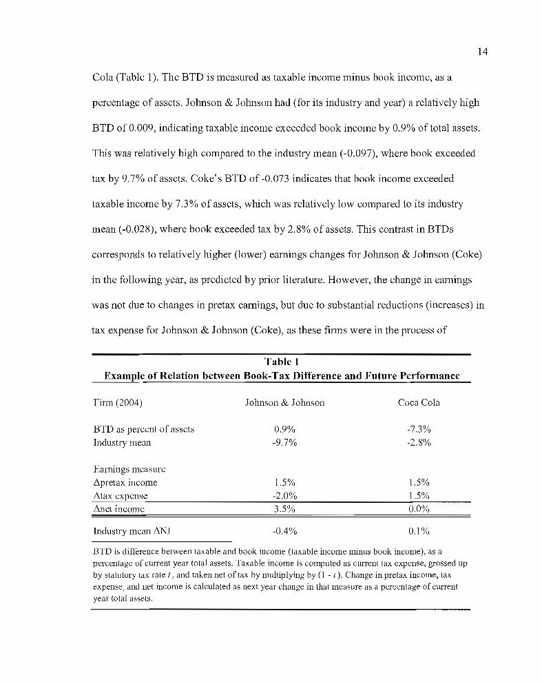
14

Cola (Table 1). The BTD is measured as taxable income minus book income, as a

percentage of assets. Johnson & Johnson had (for its industry and year) a relatively high

BTD of 0.009, indicating taxable income exceeded book income by 0.9% of total assets.

This was relatively high compared to the industry mean (-0.097), where book exceeded

tax by 9.7% of assets. Coke's BTD of -0.073 indicates that book income exceeded

taxable income by 7.3% of assets, which was relatively low compared to its industry

mean (-0.028), where book exceeded tax by 2.8% of assets. This contrast in BTDs

corresponds to relatively higher (lower) earnings changes for Johnson & Johnson (Coke)

in the following year, as predicted by prior literature. However, the change in earnings

was not due to changes in pretax earnings, but due to substantial reductions (increases) in

tax expense for Johnson & Johnson (Coke), as these firms were in the process of

Table 1Example of Relation between Book-Tax Difference and Future Performance

Firm (2004)

BTD as percent of assetsIndustry mean

Johnson & Johnson

0.9%-9.7%

Coca Cola

-7.3%-2.8%

Earnings measure~pretax income~tax expense~net income

Industry mean ~NI

1.5% 1.5%-2.0% 1.5%3.5% 0.0%

-0.4% 0.1%

BTD is difference between taxable and book income (taxable income minus book income), as apercentage of current year total assets. Taxable income is computed as current tax expense, grossed upby statutory tax rate t. and taken net of tax by multiplying by (1 - t). Change in pretax income, taxexpense, and net income is calculated as next year change in that measure as a percentage of currentyear total assets.

15

repatriating foreign earnings under the American Jobs Creation Act of2004. While only a

simple example, this suggests that much of the BTD/earnings growth relation may be due

in part to variation in tax rates caused by tax accruals.

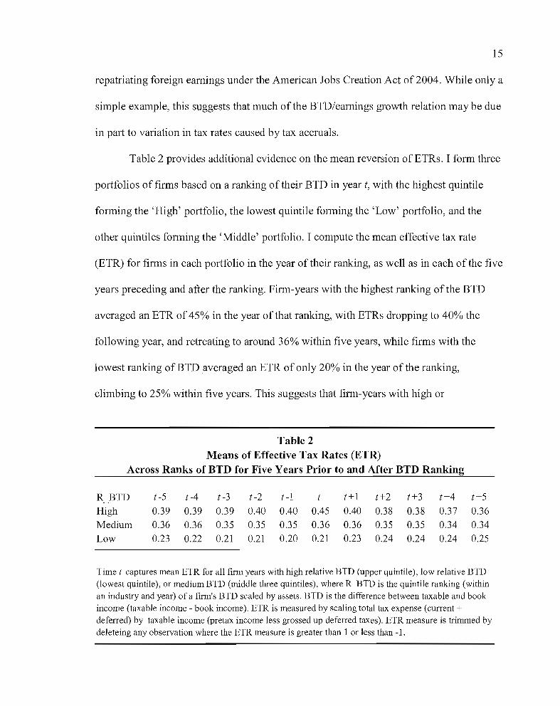
Table 2 provides additional evidence on the mean reversion of ETRs. I form three

portfolios of firms based on a ranking of their BTD in year t, with the highest quintile

forming the 'High' portfolio, the lowest quintile forming the 'Low' portfolio, and the

other quintiles forming the 'Middle' portfolio. I compute the mean effective tax rate

(ETR) for firms in each pOlifolio in the year of their ranking, as well as in each of the five

years preceding and after the ranking. Firm-years with the highest ranking of the BTD

averaged an ETR of 45% in the year of that ranking, with ETRs dropping to 40% the

following year, and retreating to around 36% within five years, while firms with the

lowest ranking ofBTD averaged an ETR of only 20% in the year of the ranking,

climbing to 25% within five years. This suggests that firm-years with high or

Table 2Means of Effective Tax Rates (ETR)

Across Ranks of BTD for Five Years Prior to and After BTD Ranking

R BTD t-5 t-4 t-3 t-2 t -1 t t+l t+2 t+3 t+4 t+5High 0.39 0.39 0.39 0.40 0.40 0.45 0.40 0.38 0.38 0.37 0.36Medium 0.36 0.36 0.35 0.35 0.35 0.36 0.36 0.35 0.35 0.34 0.34Low 0.23 0.22 0.21 0.21 0.20 0.21 0.23 0.24 0.24 0.24 0.25

Time t captures mean ETR for all firm years with high relative BTD (upper quintile), low relative BTD(lowest quintile), or medium BTD (middle three quintiles), where R_BTD is the quintile ranking (withinan industry and year) of a firm's BTD scaled by assets. BTD is the difference between taxable and bookincome (taxable income - book income). ETR is measured by scaling total tax expense (current +deferred) by taxable income (pretax income less grossed up deferred taxes). ETR measure is trimmed bydeleteing any observation where the ETR measure is greater than 1 or less than -1.

16

low rankings ofBTDs quickly experienced large changes in their ETR, which in tum

could significantly affect their future after-tax net income. To the extent these swings in

ETRs are caused by tax accruals, the positive relation between tax accruals and future

changes in net income will be largely due to the negative relation with future changes in

tax expense.

Permanent D~tlerences

The relation between future eamings changes and permanent differences is less

clear. Consider a firm with otherwise constant net income, but experiences a one-time

charge that results in a permanent book-tax difference (for example, write-off of

goodwill). This BTD will result in a relatively high effective tax rate for the level of net

income (net income was reduced by the charge, with no corresponding reduction in

taxable income). Although all other economic performance is equal, future net income

will increase due to the future absence of the one-time charge, this time related to

changes in pretax income, not changes in tax expense. 7 Thus, some pennanent

differences simply capture transitory economic events that naturally affect future eamings

changes by failing to repeat. Consider now a firm with otherwise constant net income, but

with pennanent differences that are not transitory (such as dividends regularly received

from another firm, which are largely excluded from taxable income). As long as the

permanent difference is constant, there is no reason to expect a change in future net

7 The argument could be made that future economic perfonnance will not be equal. The write-down ofgoodwill may well predict future declines in economic perfonnance. Ultimately the impact oftransitory pennanent differences on future pretax earnings changes is an empirical question.

17

income from pretax changes or from tax expense variation. In this case, permanent BTDs

have no relation to future earnings growth.

The previous examples demonstrate that BTDs generated by tax accruals lead to

tax expense changes, while permanent differences may be related to future changes in

pretax earnings in either direction, or they may have no relation at all to pretax earnings

changes. The third type ofBTD, temporary differences, is the most easily separated from

the other two (as it is reported as deferred tax), and will be discussed below. Controlling

for temporary differences, I propose that the relation between the non-temporary

components of BTDs and future earnings changes is due primarily to future changes in

tax expense. My first hypothesis is:

HI: There is a negative relation between the non-temporary components of

BTDs (tax accruals and permanent differences) and future tax expense.

Temporary Differences

Temporary differences (identified by the deferred tax expense) capture income or

expense items that are recognized at different times for book and tax purposes. These

timing differences can be useful in identifying managerial discretion in accounting

decisions. For example, managers exercise judgment with respect to depreciation periods

and methods, revenue recognition, and recording reserve allowances such as bad debt,

warranties, and contingencies. To the extent that management exercises its discretion in

these matters to inflate (reduce) income for financial reporting purposes, the reversing

nature of accruals dictates that any resulting temporary BTDs will be associated with

18

future declines (increases) in pretax earnings. This is true for at least two reasons. First,

all else equal, the earnings in a year following one with inflated earnings will lower by

definition. Second, accruals reverse, so to the extent that temporary BTDs capture

accrual-based earnings management, the reversal of these managed accruals in a

subsequent year will cause future income to be lower.

Management discretion in financial reporting also serves as a signal of

management's private information about future firm performance. Consider a firm in

distress that provides for a large valuation allowance against its deferred tax assets. 8 This

creates a temporary difference reflected in a deferred tax expense, and this temporary

difference is informative about future declines in economic performance. 9 Hence,

whether temporary differences reflect the discretion in accruals used to manipulate

earnings, or rather reveals management's private information through the discretion in

accruals, there is reason to expect a negative relation between future earnings and

temporary differences. Hanlon (2005) finds that the pretax earnings of firms with large

temporary BTDs are less persistent. In contrast, Lev and Nissim (2004) find no relation

between net income growth and temporary differences. I predict that pretax earnings

8 As discussed previously, the valuation allowance account is a tax accrual, but because it is measuredby deferred taxes, it is treated as a temporary difference, both in the hypothesis development and inthe empirical tests.

9 There are cases where the creation of a deferred tax asset would predict future declines in economicperformance. For example, consider a finn constant in size, but with changes in its allowance fordoubtful accounts or warranty liabilities. These changes will generate deferred tax assets that are alsoinformative about future firm prospects, as it contains infonnation about management's assessment offuture collectability of receivables or quality of goods sold. Ultimately it is an empirical questionwhether deferred tax expense, absent earnings management, predicts higher or lower growth.

19

growth for firms with large temporary differences will be lower. My second hypothesis

IS:

H2: Large temporary BTDs (deferred taxes) are negatively related to growth in

pretax earnings.

Finding empirical support for H2 suggests that temporary differences are related

to future changes in pretax income, but provides no evidence as to the nature of the

causality of this relation. As discussed above, manipulated earnings numbers can lead to

temporary BTDs that will be related to lower future earnings growth. However,

underlying economic events and conditions can also result in temporary BTDs that are

related to future earnings growth. In the example noted above, a change in the valuation

allowance account results in a change in deferred taxes that is informative about future

finn prospects. Similarly, consider a firm with significant unearned revenue that is

recognized as income for tax purposes. This will result in a deferred tax asset (a negative

deferred tax expense), which will be related to future book revenue (when the previously

unearned revenue is recognized). Thus, I predict that even in the absence of earnings

management, temporary BTDs, as measured by the deferred tax expense, will be

negatively related to growth in pretax earnings, and that the relation between temporary

differences and future pretax earnings growth will be stronger in finn-years suspected of

earnings management. Addressing the causality of the relation predicted in H2, my third

set of hypotheses are:

20

H3a: In the absence of earnings management, temporary differences are

negatively related to pretax earnings growth.

H3b: The negative relation between temporary differences and pretax earnings

growth is stronger in the presence of earnings management.

HI predicts a negative relation between permanent differences and future changes

in tax expense. However, finding empirical support for HI provides no evidence as to the

nature of the causality of this relation. As discussed in HI, the non-temporary

components of total BTDs are composed of both tax accruals (not including the valuation

allowance account) and permanent differences. While it is unclear how permanent

differences are used in earnings management, prior research has provided evidence that

tax accruals have been used to manage earnings. The manipulation of these accruals do

not affect pretax earnings, but only affects tax expense, so I expect that firms suspected

of earnings management will have a stronger negative relation between non-temporary

BTDs and future tax expense changes. However, even in the absence of earnings

management, I expect a negative relation between the non-temporary differences and

future tax expense changes as the tax expense mean reverts towards the statutory tax rate.

Consider an international firm with constant earnings. For economic reasons (investment

opportunities domestically and abroad), the firm in year one repatriates its foreign

earnings, resulting in a relatively high amount of cunent tax expense compared to its

book income (and thus a higher BTD). In the following year the firm designates its

foreign earnings as permanently reinvested (PRE), escaping the repatriation tax expense,

and hence its net income has increased due to a tax expense decrease, all related to the

21

relatively high BTD from year one. This relation occurs in the absence of earnings

management objectives. However, Krull (2004) demonstrates that the PRE designation is

used to manage earnings, so in the presence of earnings management, I expect the

relation between tax accruals and future changes in tax expense to be even stronger.

Addressing the causality of the relation predicted in HI, my final set of hypotheses are:

H4a: In the absence of earnings management there is a negative relation

between non-temporary BTDs and future tax expense changes.

H4b: The negative relation between non-temporary BTDs and future tax

expense changes is stronger in the presence of earnings management.

22

CHAPTER IV

RESEARCH DESIGN

To test the relation between the components ofBTDs and earnings changes, I first

measure the temporary and permanent components of BTDs with the following

procedure introduced by Weber (2008): First, I estimate TAXDIFF (total BTDs) as the

difference between taxable income and net income, scaled by total assets,

TAXDIFF = (taxable income - net income) / average assets (1)

where net income is measured as income before extraordinary items (Compustat #18) and

average assets is the mean total assets (Compustat #6) over the previous two years.

Taxable income is estimated by grossing up current tax expense,

Taxable income = current tax expense / t * (l-t) / average assets (2)

where the current portion of the income tax expense is grossed up by t, the top statutory

corporate federal tax rate. 10 Taxable Income is multiplied by (1 - t) to make it

comparable to Net Income, which is measured after tax.! I I then estimate TEMP, the

temporary component of total BTDs, by grossing up the negative of deferred taxes,

]0 The top statutory corporate tax rate was 48% in 1973-1978,46% in 1979-1986,40% in 1987,34%in 1988-1992, and 35% in 1993-2006.

11 The estimate of taxable income contains measurement error from several sources, such as the use ofthe top statutory tax rate in a progressive system or to represent foreign tax rates, the misalignment oftax expense and benefits for stock options, and tax credits (See Manzon and Plesko (2002), Mills,Newberry, and Trautman (2002), McGill and Outslay (2002), Hanlon (2003) Mills and Plesko (2003),

TEMP = - (deferred tax expense) / t * (1-t) / average assets

23

(3)

where the negative of deferred taxes are grossed up by t, multiplied by (1 - t), and scaled

by total assets, making it comparable in measurement to Taxable Income. Because

TAXDlFF captures the extent to which taxable income exceeds book income, I use the

negative of deferred tax, which otherwise would capture the extent to which bo?k income

exceeds taxable income. Finally, I estimate PERM, the non-temporary component of total

BTDs (permanent differences and tax accruals), as the difference between TAXDlFF and

TEMP. 12

PERM = TAXDIFF- TEMP

This procedure captures the extent to which taxable income exceeds book income,

breaking this difference into permanent and temporary components.

(4)

and Lev and Nissim (2004) for a discussion of the measurement error in estimates of taxable income).However, Lev and Nissim (2004) use the same estimate of taxable income in the computation of theirtax to book ratio (TAX) and find that these errors do not systematically affect the relation between theTAX ratio and growth in net income.

12 This is a key departure from the Lev and Nissim (2004) methodology due to the difficulty ininterpreting their coefficients. Their key variables are R_TAX and R_DEF, the quintile ranks of thetaxlbook ratio and deferred taxes. Conceptually, TAX captures total BTDs, while DEF capturestemporary differences, making DEF a subset of TAX. When both are included in a regression, thecoefficient on TAX will capture the effect of permanent differences and tax accruals on growth, whilethe sum of the coefficients on TAX and DEF will reflect the impact of temporary differences. Hence, alack of significance on DEF alone would not necessarily indicate that temporary differences do notpredict earnings growth. However, because TAX is measured as a ratio, while DEF is the temporarycomponent scaled by assets, DEF is no longer strictly a subset of TAX, and the interpretation of thecoefficients on these variables (or their ranks) is unclear. My method of splitting the total BTD into itstwo components provides two variables that are not subsets of each other, but in sum capture the totalBTD. The coefficient on PERM now clearly captures the impact of pennanent differences and taxaccruals, while the coefficient on TEMP relates only to the impact of temporary differences.

24

I then estimate the relation between the components of BTDs and earning changes

with the following equation:

L"1NI = a + ~lPERM + ~2TEMP + ICONTROLS + E (5)

where L"1NI is an indicator of future changes in net income. It is alternatively measured as:

next year's net income minus current net income (L"1NI 1), average net income over the

next three years minus current net income (L"1NI 3), and average net income over the next

five years minus current net income (L"1NI 5)' Net income is measured as Compustat #18

(income before extraordinary items) scaled by total assets (#6).

Because many BTDs result from accrual estimates, it could be argued that any

relation between BTDs and growth simply proxies for the effect that accruals have on

earnings growth. To examine whether permanent differences (PERM) or temporary

differences (TEMP) contain incremental infoTInation relative to accruals and cash flows, I

include two related control variables, ACC and CASH 13, estimated as total accruals and

total cash from operations, respectively, each scaled by total assets. 14 In this way, the

coefficients on PERM and TEMP should capture the information in peTInanent

differences and temporary differences incremental to each other and to accruals about

future changes in net income.

13 Cash from operations is measured as the difference between income (before extraordinary items)and accruals, where accruals = (L'1cunent assets - L'1cash) - (L'1cunent liabilities - L'1short-tenn debt) ­L'1defened tax liabilities - depreciation.

14 This is similar in spirit to Lev and Nissim's (2004) CFO measure, the percentage of net income dueto cash flows. However, the CFO measure is scaled by net income, which does not allow thiscash/accrual measure to compete on an even footing with PERM and TEMP, which are scaled by totalassets.

25

Chan, Karceski, and Lakonishok (2003) and Fama and French (2000) identify

several other predictors of earnings growth. Following Lev and Nissim (2004), I add the

following control variables: current change in ROA, average change in ROA over three

and five years, dividends scaled by assets, the ratios of R&D to sales and capital

expenditures to sales, and the current earnings I price (E/P) ratio and book-to-market

(BTM) ratio. 15 Current and longer term changes in ROA control for short and long term

trends in earnings, and should be positively related to future earnings changes. The level

of dividends may reflect management's confidence in future earnings strength,

suggesting a positive relation with future earnings changes, or it may signal fewer

investment opportunities for the firm, suggesting a negative relation with future earnings.

changes. The ratios of R&D and capital expenditures to sales controls for expected sales

growth due to new investments, but it also identifies growing firms making large

investment outlays whose profitability may not improve in the short tenn, so I do not

make a prediction on these variables. The E/P and BTM ratios capture market

expectations of future growth. Each has stock price in the denominator, so that higher

stock prices (and higher market expectations for earnings growth) will result in lower

values for these ratios. Thus I expect an inverse relation between these ratios and future

changes in earnings growth.

15 Lev and Nissim (2004) also include current return on assets, controlling for the tendency ofprofitability to mean revert. However, I have already captured ROA with the ACC and CASHvariables, whose numerators add to total net income, and whose denominator is total assets.

26

To examine the statistical significance of the relation between the BTD measures

and the two components of earnings changes, I estimate the following two additional

equations:

L'.PRETAX = a + ~lPERM + ~2TEMP + ~CONTROLS + E

L'.TAXEXP = a + ~lPERM + ~2TEMP + ~CONTROLS + E

where L'.PRETAX captures future changes in pretax earnings, and L'.TAXEXP captures

(6)

(7)

future changes in tax expense. Following Hanlon (2005), PRETAX is measured as pretax

income less minority interest scaled by average total assets. TAXEXP is measured as

total income tax expense scaled by total assets. As with the variation on L'.NI, L'.PRETAX

is alternatively measured as: next year's pretax earnings minus current pretax earnings

(L'.PRETAX 1), average pretax earnings over next three years minus current pretax

earnings (L'.PRETAX 3), and average pretax earnings over next five years minus current

pretax earnings (L'.PRETAX 5)' The three estimates ofTAXEXP are measured in the same

way. To the extent permanent and temporary differences are positively related to changes

in pretax earnings, the coefficients on PERM and TEMP will be positive in the estimates

of equation (6). H2 predicts a positive coefficient on TEMP, as temporary differences

(the extent to which taxable income is greater than book income due to timing

differences) are predicted to be positively related to future pretax earnings changes. 16 If

16 Note that H2 predicts a negative relation between deferred tax and future pretax earnings. To beconsistent with the measurement of PERM and TAXDlFF

, which measure the extent to which taxable

27

the BTD measures are negatively related to changes in tax expense, then the coefficients

will be negative when estimating equation (7). HI predicts a negative coefficient on

PERM when estimating equation (7), as the tax accruals component of PERM is expected

to be related to declines in tax expense.

If a component ofBTDs predicts eamings growth, it could reflect the influence

of current eamings management activities on future growth in eamings, or it may simply

reflect underlying economic events that generate various levels of BTDs and are related

to eamings growth. To examine this issue, I identify finn-year observations where

eamings management is suspected and create a dummy indicator (EM) equal to one for

these finn years, and zero for finns that have no evidence of eamings management.

Similar to Phillips, Pincus, and Rego (2003), I use four different proxies for eamings

management: avoiding an eamings decline, avoiding an eamings loss, meeting analysts'

forecasts, and high discretionary accruals. Prior work such as Burgstahler and Dichev

(1997) indicate that an abnonnally high percentage of finns have small eamings increases

or slightly positive eamings, suggesting that many finns in these categories are managing

their eamings upwards to avoid an eamings decrease or a loss. To identify eamings

management based on eamings changes, EMl =1 if the change in net income (Compustat

#172) scaled by previous year's beginning market value of equity (#25 x #199) is ~O and

<0.02, and EMI =0 otherwise. To identify eamings management based on avoiding a loss,

I compare finns with zero or slightly positive scaled eamings with those that easily

income exceeds book income, TEMP is the negative of deferred taxes scaled by assets, so theexpected coefficient on TEMP is positive.

28

attained positive earnings. Specifically, EM2=1 ifnet income scaled by beginning of year

market value is ~O and <0.02, and 0 otherwise.

Degeorge, Patel, and Zeckhauser (1999) find evidence that suggests earnings

management among firms that narrowly beat analysts' forecasts. To identify earnings

management with analysts' forecasts, I identify firms that meet or narrowly beat their

forecast. Specifically, EM3=1 if the earnings surprise (actual IBES earnings per share-

consensus forecast) is ~O and less than 0.02, and EM3=0 otherwise. I?

Discretionary accruals have also been proposed as a means of identifying earnings

management. I follow the modified Jones model proposed by Dechow, Sloan, and

Sweeney (1995) to identify discretionary accruals. I estimate the following equation:

Accruals = a + ~l(l/A) + ~2C~REV-~REC) + ~3(PPE) + E

where accruals are as measured earlier, A is total assets, ~REV is change in revenue

(Compustat #12), ~REC is change in receivables (#2), and PPE is property, plant, and

equipment (#7), each scaled by total assets (#6). Equation (4) is estimated cross-

sectionally each year for each two-digit SIC code. The residuals from this equation are

(8)

categorized as discretionary accruals, and I then rank the residuals into quintiles. I set the

earnings management indicator EM4=1 for firms with the highest quintile rank of

discretionary accruals, and 0 otherwise.

17 In sensitivity tests, I use various other thresholds for 'small' earnings changes, 'slightly' positiveearnings, and 'narrowly' beating analysts' forecasts. Results are substantially unchanged.

29

With these proxies for earnings management, I then re-estimate equations (1), (2),

and (3), including the EM dummy alone and interacted with the rank variables for non­

temporary BTDs (PERM), temporary BTDs (TEMP), and all control variables:

i'1NI = a + ~lPERM + P2TEMP + P3EM + P4EM*PERM +

~5EM*TEMP + LCONTROLS + EM*LCONTROLS + £

i'1PRETAX = a + P1PERM + ~2TEMP + ~3EM + ~4EM*PERM +

~5EM*TEMP + LCONTROLS + EM*LCONTROLS + £

i'1TAXEXP = a + ~IPERM + ~2TEMP + ~3EM + ~4EM*PERM +

~5EM*TEMP + LCONTROLS + EM*LCONTROLS + £

(9)

(10)

(11 )

where i'1NI, i'1PRETAX, and i'1TAXEXP are alternatively measured over one, three, and

five year periods as before, and EM is alternatively identified as suspected earnings

management finn-years based on earning changes, earnings levels, analysts' forecasts, or

discretionary accruals. I continue to control for growth related variables as discussed

earlier, and each independent variable is interacted with the EM dummy. If finns that

manage earnings are expected to have less future growth, ~3 will be negative. As

predicted by H3a and H4a, if the relation between BTDs and earnings changes is not only

an artifact of earnings management, but has underlying economic causes, the coefficient

on TEMP in equation (10) will be positive, and the coefficient on PERM in equation (11)

will be negative. As predicted by H3b and H4b, if earnings management intensifies the

magnitude of the BTD/growth relationship, the coefficient on EM*TEMP in equation

(10) will be positive, and the coefficient on EM*PERM in equation (11) will be negative.

30

CHAPTER V

SAMPLE AND SUMMARY STATISTICS

Sample Selection

I draw my sample from the annual Compustat files for years 1973-2006. I restrict

my sample to firms that are incorporated in the U.S. (Compustat FINC=O), are not a

financial, utility, or flow-through entity (SIC codes 4000s and 6000s), and have a

December year-end (FYR=12). These restrictions are necessary as foreign-incorporated

firms face different accounting and tax rules, utilities and financial institutions face

different regulatory and reporting rules, and flow-through entities do not pay tax.

Requiring a common fiscal year controls for temporal fluctuations in the economy.

Because domestic and foreign components of current and deferred tax are not widely

available on Compustat before 1973, I begin my sample selection in that year.

To perfonn my tests, my initial sample includes only observations that have the

following data: Total assets (Compustat #6), total income tax (#16), income before

extraordinary items (#18), number of shares outstanding (#25), deferred taxes (#50),

common equity (#60), and price per share (#199). Due to the difficulty of interpreting

BTDs for firms with negative income and taxes, I include only observations with positive

net income and tax expense. 18 This selection procedure results in a base sample of 49,956

finn-year observations, representing 6,837 different finns over the 34-year period 1973­

2006. To mitigate the influence of extreme observations, I delete from each analysis

]8 In sensitivity tests I relax this restriction, with no change in results.

31

observations in which any continuous variable lies beyond the highest and lowest 0.5% of

the distribution for that variable. 19

Summary Statistics

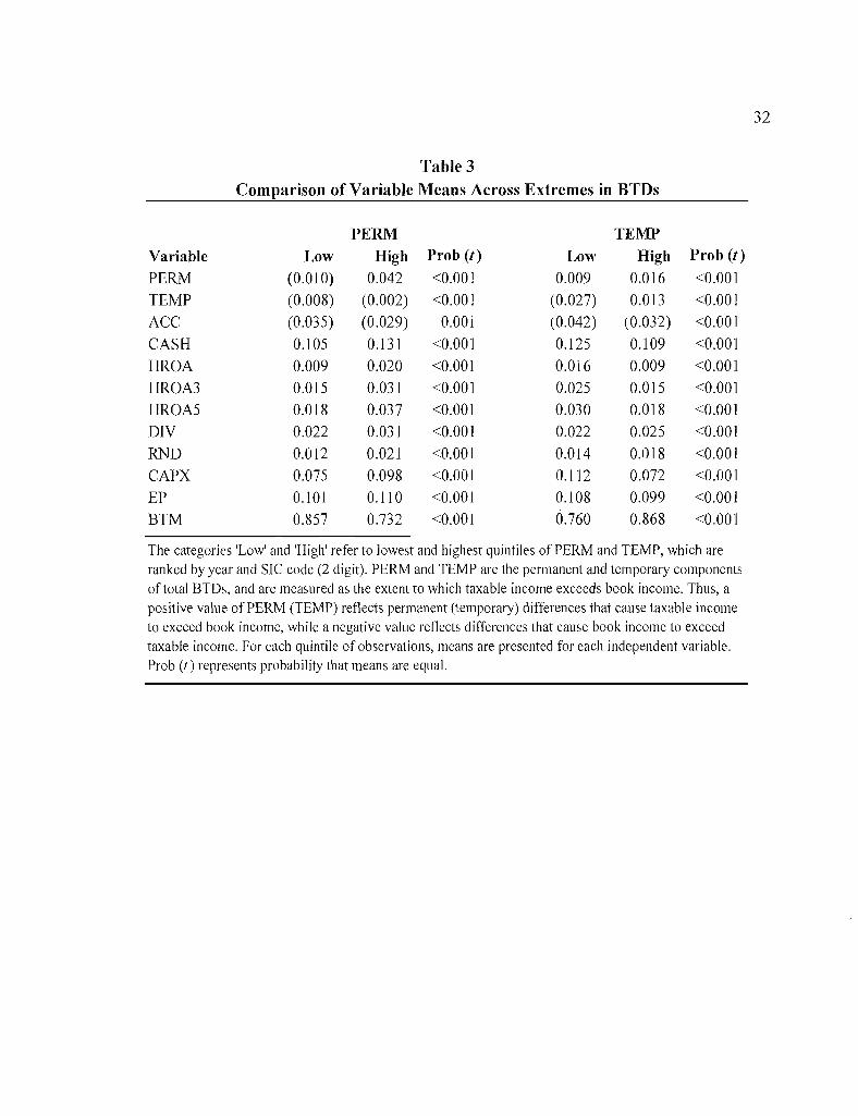
Table 3 presents a comparison ofmeans of the independent variables (including

the control variables for growth) across high and low quinti1e ranks of the PERM and

TEMP variables. The means are significantly different for all of these variables across

different quinti1es. This highlights how these firms are fundamentally different from one

another depending on their level ofpermanent or temporary BTDs and the importance of

controlling for these growth proxies when determining the impact ofBTDs on future

earnings growth. Table 4 presents a correlation matrix for these variables. As expected,

there is a high degree of correlation between changes in net income, changes in pretax

income, and changes in tax expense. As predicted by H2, there is a positive correlation

between temporary BTDs and changes in pretax income. In contrast to expectations, there

is a positive correlation between permanent BTDs and changes in tax expense. However,

the high degree of correlation between the dependent and independent variables makes

inference difficult in a univariate setting, highlighting the need for multivariate tests.

19 An exception to this is R&D expenditures. Because I set this variable to zero if missing inCompustat, over half of the observations have zero R&D, and selecting a lower 0.5% to delete is notfeasible. I do exclude observations with R&D in the upper 0.5% of the distribution for regressionsincluding this variable.

32

Table 3Comparison of Variable Means Across Extremes in BTDs

VariablePERM

TEMP

ACCCASHHROA

HROA3

HROA5

DIYRND

CAPXEP

BTM

Low(0.010)

(0.008)

(0.035)

0.105

0.009

0.015

0.018

0.022

0.012

0.075

0.101

0.857

PERMHigh

0.042

(0.002)

(0.029)

0.131

0.020

0.031

0.037

0.031

0.021

0.098

0.110

0.732

Prob (t)

<0.001

<0.001

0.001

<0.001

<0.001

<0.001

<0.001

<0.001

<0.001

<0.001

<0.001

<0.001

Low0.009

(0.027)

(0.042)

0.125

0.016

0.025

0.030

0.022

0.014

0.112

0.108

0.760

TEMPHigh

0.016

0.013

(0.032)

0.109

0.009

0.015

0.018

0.025

0.018

0.072

0.099

0.868

Prob (t)

<0.001

<0.001

<0.001

<0.001

<0.001

<0.001

<0.001

<0.001

<0.001

<0.001

<0.00 1

<0.001

The categories 'Low' and 'High' refer to lowest and highest quintiles of PERM and TEMP, which areranked by year and SIC code (2 digit). PERM and TEMP are the permanent and temporary componentsof total BTDs, and are measured as the extent to which taxable income exceeds book income. Thus, apositive value of PERM (TEMP) reflects permanent (temporary) differences that cause taxable incometo exceed book income, while a negative value reflects differences that cause book income to exceedtaxable income. For each quintile of observations, means are presented for each independent variable.Prob (t) represents probabil ity that means are equal.

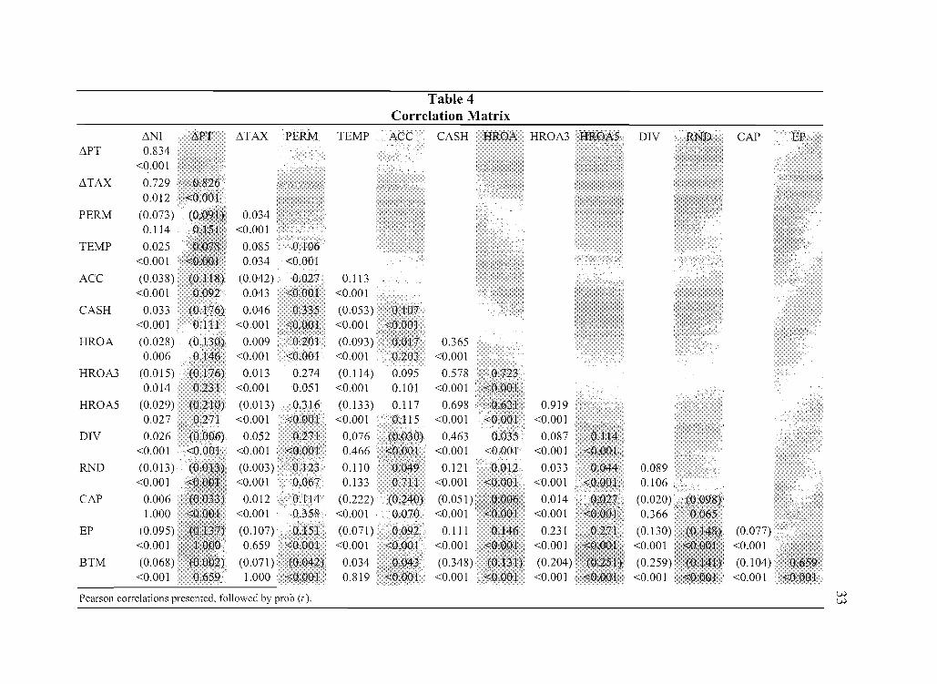
Table 4Correlation Matrix

t.NI t.PT t.TAX PERM TEMPllPT 0.834

<0.001

llTAX 0.7290.012

PERM (0.073)0.114

TEMP 0.025<0.001

ACC (0.038) (0.118) (0.042) 0.027 0.113<0.001 0.092 0.043 <0.001 <0.001

CASH 0.033 (0.176) 0.046 (0.053 )<0.001 0.111 <0.001 <0.001

HROA (0.028) 0.009 (0.093 ) 0.3650.006 <0.001 <0.001 <0.001 0.203 <0.001

HROA3 (0.015) 0.013 0.274 (0.114) 0.095 0.5780.014 0.231 <0.001 0.051 <0.001 0.101 <0.001

HROA5 (0.029) (0:210) (0.013) 0.316 (0.133) 0.117 0.698 0.9190.027 <0.001 <0.001 <0.001 15 <0.001 <0.001

DIV 0.026 0.052 0.271 0.076 0.463 0.087<0.001 <0.001 0.466 <0.001 <0.001 <0.001

RND (0.013) (0.003 ) 0.110 0.121 0.012 0.033 0.089<0.001 <0.001 0.133 <0.001 <0.001 <0.001 0.106

CAP 0.006 0.012 (0.222) (0.051 ) 0.014 (0.020)1.000 <0.001 <0.001 <0.001 <0.001 0.366

EP (0.095) (0.107) (0.071 ) 0.111 0.231 (0.130)<0.001 0.659 <0.001 <0.001 <0.001 <0.001

BTM (0.068) (0.071 ) 0.034 (0.348) (0.204) (0.259)<0.001 1.000 0.819 <0.001 <0.001 <0.001

Pearson correlations presented, followed by prob (t).WW

34

CHAPTER VI

EMPIRICAL RESULTS

The Association between Book-Tax D~frerencesand Earnings Changes

Table 5 presents results from cross-sectional regressions of equations (5), (6), and

(7). To control for differences across time and across industries, year and industry (two

digit SIC code) fixed effects are included in all tests. The first three columns present

results from using net income as the measure of earnings growth. Similar to the findings

of Lev and Nissim (2004), I find that PERM is positively and strongly related to

subsequent growth in net income over one, three, and five year periods. In contrast to the

finding of Lev and Nissim (2004), TEMP is also positively related to changes in net

income, although the coefficients on TEMP are significantly smaller than those on

PERM.20 The following three columns of Table 5 present evidence on the association

between pretax earnings growth and the pennanent and temporary components ofBTDs.

Consistent with H2, TEMP is positively and strongly related to subsequent changes in

pretax earnings over one, three, and five year periods, suggesting that the temporary

component ofBTDs, deferred tax, is negatively related to future changes in pretax

earnings.21 Interestingly, PERM is only weakly related to future pretax earnings change

20 A test of the difference in coefficients on PERM and TEMP for earnings changes over 1, 3, and 5years report F-statistics of 2.53, 21.90, and 21.25 (p=O.ll, <0.001, and <0.001).

21 Because TEMP is measured as the negative of deferred tax expense, a positive coefficient on TEMPimplies a negative relation between deferred tax and future pretax earnings changes.

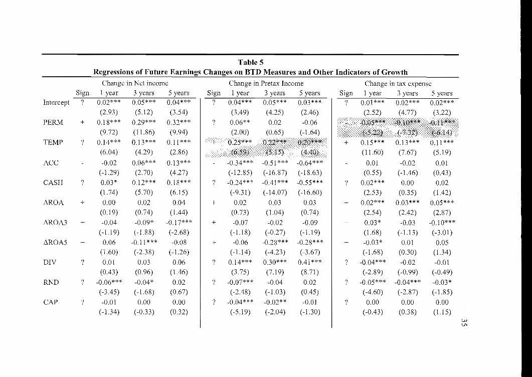
Table 5Regressions of Future Earnings Changes on BTD Measures and Other Indicators of Growth

Change in Net income Change in Pretax Income Change in tax expense

Sign 1 year 3 years 5 years Sign 1 year 3 years 5 years Sign 1 year 3 years 5 years

Intercept ? 0.02*** 0.05*** 0.04*** ? 0.04*** 0.05*** 0.03***

I? 0.01 *** 0.02*** 0.02***

(2.93) (5.12) (3.54) (3.49) (4.25) (2.46) (2.52) (4.77) (3.22)

PERM + 0.18*** 0.29*** 0.32*** ? 0.06** 0.02 -0.06

(9.72) (11.86) (9.94) (2.00) (0.65) (-1.64)

TEMP ? 0.14*** 0.13*** 0.11 *** + 0.15*** 0.13*** 0.11 ***

(6.04) (4.29) (2.86) (11.60) (7.67) (5.19)

ACC -0.02 0.06*** 0.13*** - -0.34*** -0.51 *** -0.64*** - 0.01 -0.02 0.01

(-1.29) (2.70) (4.27) (-12.85) (-16.87) (-18.63) (0.55) (-1.46) (0.43)

CASH ? 0.03* 0.12*** 0.18*** ? -0.24*** -0.41*** -0.55*** ? 0.02*** 0.00 0.02

(1.74) (5.70) (6.15) (-9.31) (-14.07) (-16.60) (2.53) (0.35) (1.42)

flROA + 0.00 0.02 0.04 + 0.02 0.03 0.03 + 0.02*** 0.03*** 0.05***

(0.19) (0.74) (1.44) (0.73) (1.04) (0.74) (2.54) (2.42) (2.87)

flROA3 + -0.04 -0.09* -0.17*** + -0.07 -0.02 -0.09 + 0.03* -0.03 -0.1 0***

(-1.19) (-1.88) (-2.68) (-1.18) (-0.27) (-1.19) (1.68) (-1.13) (-3.01)

flROA5 + 0.06 -0.11 *** -0.08 + -0.06 -0.28*** -0.28*** + -0.03* 0.01 0.05

(1.60) (-2.38) (-1.26) (-1.14) (-4.23) (-3.67) (-1.68) (0.30) (1.34)

DIV ? 0.01 0.03 0.06 ? 0.14*** 0.30*** 0.41*** ? -0.04*** -0.02 -0.01

(0.43) (0.96) (1.46) (3.75) (7.19) (8.71) (-2.89) (-0.99) (-0.49)

RND ? -0.06*** -0.04* 0.02 ? -0.07*** -0.04 0.02 ? -0.05*** -0.04*** -0.03*

(-3.45) (-1.68) (0.67) (-2.48) (-1.03) (0.45) (-4.60) (-2.87) (-1.85)

CAP ? -0.01 0.00 0.00 ? -0.04*** -0.02** -0.01 ? 0.00 0.00 0.00

(-1.34) (-0.33) (0.32) (-5.19) (-2.04) (-1.30) (-0.43) (0.38) (1.15)t.NVI

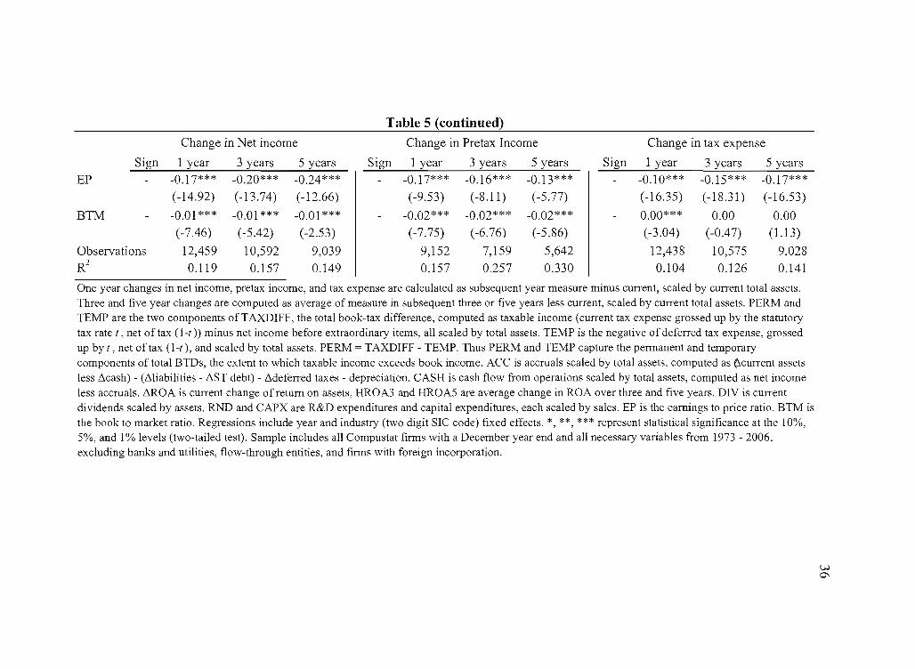
Table 5 (continued)

Change in Net income Change in Pretax [ncome Change in tax expense

Sign 1 year 3 years 5 years Sign 1 year 3 years 5 years Sign 1 year 3 years 5 years

EP -0.17*** -0.20*** -0.24*** - -0.17*** -0.16*** -0.13*** - -0.10*** -0.15*** -0.17***(-14.92) (-13.74) (-12.66) (-9.53) (-8.11) (-5.77) (-16.35) (-18.31) (-16.53)

BTM - -0.01 *** -0.01 *** -0.01 *** - -0.02*** -0.02*** -0.02*** - 0.00*** 0.00 0.00(-7.46) (-5.42) (-2.53 ) (-7.75) (-6.76) (-5.86) (-3.04) (-0.47) (1.13)

Observations 12,459 10,592 9,039 9,152 7,159 5,642 12,438 10,575 9,028R2

0.119 0.157 0.149 0.157 0.257 0.330 0.104 0.126 0.141

One year changes in net income, pretax income, and tax expense are calculated as subsequent year measure minus current, scaled by current total assets.Three and five year changes are computed as average of measure in subsequent three or five years less current, scaled by current total assets. PERM andTEMP are the two components ofTAXDIFF, the total book-tax difference, computed as taxable income (current tax expense grossed up by the statutorytax rate t, net of tax (l-t)) minus net income before extraordinary items, all scaled by total assets. TEMP is the negative of deferred tax expense, grossedup by t , net of tax (1-t), and scaled by total assets. PERM = TAXDIFF - TEMP. Thus PERM and TEMP capture the permanent and temporarycomponents of total BTDs, the extent to which taxable income exceeds book income. ACC is accruals scaled by total assets, computed as (lcurrent assetsless ~cash) - (~liabilities - ~ST debt) - ~deferred taxes - depreciation. CASH is cash flow from operations scaled by total assets, computed as net incomeless accruals. ~ROA is current change ofreturn on assets, HROA3 and HROA5 are average change in ROA over three and five years. DIV is currentdividends scaled by assets. RND and CAPX are R&D expenditures and capital expenditures, each scaled by sales. EP is the earnings to price ratio. BTM isthe book to market ratio. Regressions include year and industry (two digit SIC code) fixed effects. *, **, *** represent statistical significance at the 10%,5%, and I% levels (two-tailed test). Sample includes all Compustat firms with a December year end and all necessary variables from 1973 - 2006,excluding banks and utilities, flow-through entities, and firms with foreign incorporation.

VJ0\

37

in the following year, and there is no evidence of a relation over three or five years.

The final three columns of Table 5 present evidence on the association between

changes in tax expense and the permanent and temporary components of BTDs.

Consistent with HI, PERM is negatively and strongly related to changes in tax expense

over one, three, and five year periods. This result suggests that any relation between

permanent BTDs and future earnings changes are due to changes in future tax expense,

not changes in the underlying (pretax) earnings of the firm. The final three columns of

Table 5 also reveal a positive and significant relationship between TEMP and tax expense

changes. This is not unexpected, as TEMP is positively associated with pretax earnings,

and increases in pretax earnings should lead to increases in tax expense, ceteris paribus.

Impact ofEarnings Management on Association between Book-Tax D~fferencesand

Earnings Growth

Tables 6-9 examine the impact of earnings management on the documented

association between BTDs and earnings changes. I use various proxies for earnings

management, including narrowly avoiding an earnings decline (Table 6), narrowly

avoiding a loss (Table 7), meeting or narrowly beating analysts' forecasts (Table 8), and a

high level of discretionary accruals (Table 9). H3a predicts that even in the absence of

earnings management there will be a positive relation between temporary BTDs and

changes in pretax earnings, i.e., the coefficient on TEMP is positive when 1'.PRETAX is

the dependent variable. H3b predicts that earnings management activity will intensify this

association, i.e., the interaction of TEMP with an earnings management dummy is

positive when 1'.PRETAX is the dependent variable. H4a predicts that even in the absence

38

of earnings management there will be a negative relation between non-temporary BTDs

and changes in tax expense (due to the impact tax accruals have on ETR swings), i.e., the

coefficient on PERM is negative when L1TAXEXP is the dependent variable. H4b

predicts that earnings management activity will intensify this association, i.e., the

coefficient on the interaction of PERM with an earnings management dummy is negative.

I begin by defining earnings management on the basis of annual earnings changes.

I define an earnings management dummy EM=1 when the change in earnings (scaled by

market value of equity) is greater than or equal to zero, but less than two cents, with

EM=O otherwise. I then include the EM dummy variable alone and interacted with each

independent variable as outlined in equations (9), (10), and (11). Table 6 presents the

results. Consistent with H3a and H4a, the positive (negative) coefficient on TEMP

(PERM) suggests that the relation documented earlier between the BTD measures and

L1PRETAX (1'1TAXEXP) hold even in the absence of earnings management. Inconsistent

with H3b and H4b, there is no evidence of statistical significance on the interaction terms

of EM with TEMP and PERM. This suggests that the BTD/earnings change relation is

not a product of this type of earnings management.

I next examine earnings management defined as avoidance of losses. I define

EM=1 when net income scaled by market value of equity is greater or equal to zero, but

less than two cents. I include the EM dummy variable alone and interacted with each

independent variable as outlined in equations (9), (10), and (11). Table 7 presents the

results. Consistent with H3a and H4a, the positive (negative) coefficient on TEMP

(PERM) suggests that the relation documented earlier between the BTD measures and

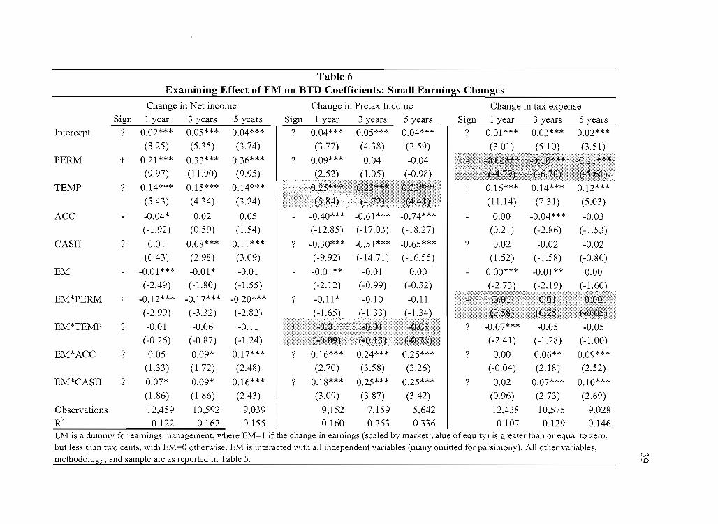
Table 6Examining Effect of EM on BTD Coefficients: Small Earnings Changes

Change in Net income Change in Pretax Income Change in tax expenseSign 1 year 3 years 5 years Sign 1 year 3 years 5 years Sign 1 year 3 years 5 years

Intercept ? 0.02*** 0.05*** 0.04*** ? 0.04*** 0.05*** 0.04*** ? 0.01 *** 0.03*** 0.02***(3.25) (5.35) (3.74) (3.77) (4.38) (2.59)

PERM + 0.21 *** 0.33*** 0.36*** ?(9.97) (11. 90) (9.95)

TEMP ? 0.14*** 0.15*** 0.14***

(5.43) (4.34) (3.24) (11.14) (7.31) (5.03)

ACC - -0.04* 0.02 0.05 - -0.40*** -0.61 *** -0.74*** - 0.00 -0.04*** -0.03(-1.92) (0.59) (1.54) (-12.85) (-17.03) (-18.27) (0.21) (-2.86) (-1.53)

CASH ? 0.01 0.08*** 0.11 *** ? -0.30*** -0.51 *** -0.65*** ? 0.02 -0.02 -0.02(0.43 ) (2.98) (3.09) (-9.92) (-14.71) (-16.55) (1.52) (-1.58) (-0.80)

EM - -0.01*** -0.01 * -0.01 - -0.01** -0.01 0.00 - 0.00*** -0.01** 0.00(-2.49) (-1.80) (-1.55) (-2.12) (-0.99) (-0.32) 1

EM*PERM + -0.12*** -0.17*** -0.20*** ? -0.11 * -0.10 -0.11(-2.99) (-3.32) (-2.82)

EM*TEMP ? -0.01 -0.06 -0.11 ? -0.07*** -0.05 -0.05(-0.26) (-0.87) (-1.24) (-2.41) (-1.28) (-1.00)

EM*ACC ? 0.05 0.09* 0.17*** ? 0.16*** 0.24*** 0.25*** ? 0.00 0.06** 0.09***(1.33) (1.72) (2.48) (2.70) (3.58) (3.26) (-0.04) (2.18) (2.52)

EM*CASH ? 0.07* 0.09* 0.16*** ? 0.18*** 0.25*** 0.25*** ? 0.02 0.07*** 0.10***

(1.86) (1.86) (2.43) (3.09) (3.87) (3.42) (0.96) (2.73) (2.69)

Observations 12,459 10,592 9,039

I9,152 7,159 5,642 12,438 10,575 9,028

R2 0.122 0.162 0.155 0.160 0.263 0.336 0.107 0.129 0.146EM is a dummy for earnings management, where EM= I if the change in earnings (scaled by market value of equity) is greater than or equal to zero,but less than two cents, with EM=O otherwise. EM is interacted with all independent variables (many omitted for parsimony). All other variables,methodology, and sample are as reported in Table 5. U-l

\0

Table 7Examining Effect of EM on BTD Coefficients: Narrowly Avoiding a Loss

Change in Net income Change in Pretax Income Change in tax expenseSign 1 year 3 years 5 years Sign 1 year 3 years 5 years Sign 1 year 3 years 5 years

Intercept ? 0.02*** 0.05*** 0.04*** ? 0.04*** 0.05*** 0.03***

I? 0.01 *** 0.02*** 0.02***

(2.84) (5.15) (3.49) (3.55) (4.38) (2.47) (2.45) (4.79) (3.20)

PERM + 0.18*** 0.28*** 0.32*** ? 0.06* 0.01 -0.07*

(9.34) (11.50) (9.81) (1.87) (0.28) (-1.86)

TEMP ? 0.12*** 0.10*** 0.08** + 0.14*** 0.12*** 0.09***(4.88) (3.17) (1.97) (10.52) (6.70) (4.32)

ACC - -0.01 0.06*** 0.13*** - -0.35*** -0.52*** -0.64*** - 0.01 -0.02 0.01(-0.85) (2.69) (4.28) (-12.87) (-16.58) (-17.98) (0.64) (-1.52) (0.40)

CASH ? 0.03** 0.12*** 0.18*** ? -0.25*** -0.42*** -0.55*** ? 0.02*** 0.00 0.02(1.98) (5.53) (6.06) (-9.51) (-13.88) (-16.03) (2.46) (0.16) (1.35)

EM - 0.00 -0.01 * 0.00 - -0.02** -0.04*** -0.01 - 0.00 -0.01 0.00(0.10) (-1.92) (-0.30) (-2.11) (-3.65) (-1.05) 1.1 (0.02)

EM*PERM + 0.44*** 0.42*** 0.34 ? 0.49*** 0.63*** 0.65**

(3.49) (2.72) (1.51 ) (2.30)

EM*TEMP ? 0.45*** 0.58*** 0.56*** ? 0.20*** 0.29*** 0.31***(3.82) (3.94) (2.89) (3.03) (3.41) (2.92)

EM*ACC ? 0.00 0.33** 0.38* ? 0.33* 0.45** 0.43** ? 0.03 0.16* 0.13(0.00) (2.24) (1.94) (1.92) (2.28) (1.97) (0.53) (1.87) (1.24)

EM*CASH ? 0.04 0.38*** 0.42** ? 0.36** 0.49*** 0.44** ? 0.05 0.18** 0.14(0.41) (2.66) (2.22) (2.15) (2.60) (2.11 ) (0.90) (2.23) (1.34)

Observations 12,459 10,592 9,039

I9,152 7,159 5,642 12,438 10,575 9,028

R20.127 0.160 0.151 0.162 0.261 0.333 0.107 0.129 0.143

EM is a dummy for earnings management, where EM= 1 when net income scaled by market value of equity is greater or equal to zero, but less than twocents, with EM=O otherwise. EM is interacted with all independent variables (many omitted for parsimony). All other variables, methodology, andsample are as reported in Table 5. .j:::>.

0

41

~PRETAX (~TAXEXP) hold even in the absence of earnings management. Inconsistent

with H4b, there is no apparent relation between the interaction of EM with PERM on

~TAXEXP, suggesting that this type of earnings management does not drive the negative

relation between non-temporary BTDs and tax expense changes. However, I do find

support for H3b, as there is a positive and significant relation between ~PRETAX and the

EM*TEMP interaction. This suggests that while even in the absence of earnings

management temporary differences are associated with future changes in pretax income,

the management of earnings to avoid a loss increases the intensity of this relation.

I next define EM=1 when the earnings surprise (actual EPS, as reported by IBES,

less the consensus forecast) is greater than or equal to zero but less than two cents. Table

8 presents the results. As in the case of earnings changes, I find support for H3a and H4a.

The documented relations between the BTD components and the components of earnings

changes hold even in the absence of earnings management. Also as in the case of

earnings changes, I fail to find support for H3b and H4b, suggesting that earnings

management around analysts' forecasts is not the main contributor to the relation between

BTD and earnings changes.

Finally, I set the earnings management indicator EM=1 for firms with the highest

quintile rank of discretionary accruals, and then use this indicator alone and interacted

with all each independent variable as outlined in equations (9), (10), and (11). Results are

presented in Table 9. As in the previous tests, I find support for H3a and H4a. Controlling

for earnings management, there continues to be a positive and significant relation

between TEMP and ~PRETAX, and a negative and significant relation between PERM

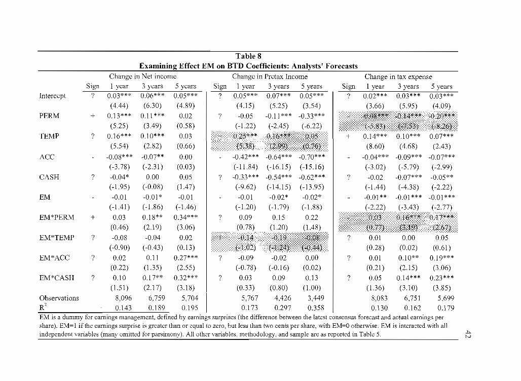
Table 8Examining Effect EM on BTD Coefficients: Analysts' Forecasts

Change in Net income Change in Pretax Income Change in tax expenseSign 1 year 3 years 5 years Sign 1 year 3 years 5 years Sign 1 year 3 years 5 years

Intercept ? 0.03*** 0.06*** 0.05*** ? 0.05*** 0.07*** 0.05***

I? 0.02*** 0.03*** 0.03***

(4.44) (6.30) (4.89) (4.15) (5.25) (3.54) (3.66) (5.95) (4.09)

PERM + 0.13*** 0.11 *** 0.02 ? -0.05 -0.11 *** -0.33***

(5.25) (3.49) (0.58) (-1.22) (-2.45) (-6.22)

TEMP ? 0.16*** 0.10*** 0.03 + 0.14*** 0.10*** 0.07***(5.54) (2.82) (0.66) (8.60) (4.68) (2.43)

ACC - -0.08*** -0.07** 0.00 - -0.42*** -0.64*** -0.70*** - -0.04*** -0.09*** -0.07***(-3.78) (-2.31) (0.03) (-11.84) (-16.15) (-15.16) (-3.02) (-5.79) (-2.99)

CASH ? -0.04* 0.00 0.05 ? -0.33*** -0.54*** -0.62*** ? -0.02 -0.07*** -0.05**(-1.95) (-0.08) (1.47) (-9.62) (-14.15) (-13.95) (-1.44) (-4.38) (-2.22)

EM - -0.01 -0.01 * -0.01 - -0.01 -0.02* -0.02* - -0.01 ** -0.01 *** -0.01 ***(-1.41) (-1.86) (-1.46) (-1.20) (-1.79) (-1.88)

EM*PERM + 0.03 0.18** 0.34*** ? 0.09 0.15 0.22

(0.46) (2.19) (3.06) (1

EM*TEMP ? -0.08 -0.04 0.02 ? 0.01 0.00 0.05(-0.90) (-0.43) (0.13) (0.28) (0.02) (0.61)

EM*ACC ? 0.02 0.11 0.27*** ? -0.09 -0.02 0.00 ? 0.01 0.10** 0.19***(0.22) (1.35) (2.55) (-0.78) (-0.16) (0.02) (0.21) (2.15) (3.06)

EM*CASH ? 0.10 0.17** 0.32*** ? 0.03 0.09 0.13 ? 0.05 0.14*** 0.23***

(1.51 ) (2.17) (3.18) (0.33) (0.80) (1.00) (1.36) (3.10) (3.85)

Observations 8,096 6,759 5,704

I5,767 4,426 3,449 8,083 6,751 5,699

R20.143 0.189 0.195 0.173 0.297 0.358 0.130 0.162 0.179

EM is a dummy for earnings management, defined by earnings surprises (the difference between the latest consensus forecast and actual earnings pershare). EM=1 if the earnings surprise is greater than or equal to zero, but less than two cents per share, with EM=O otherwise. EM is interacted with allindependent variables (many omitted for parsimony). All other variables, methodology, and sample are as reported in Table 5. -+:>.

N

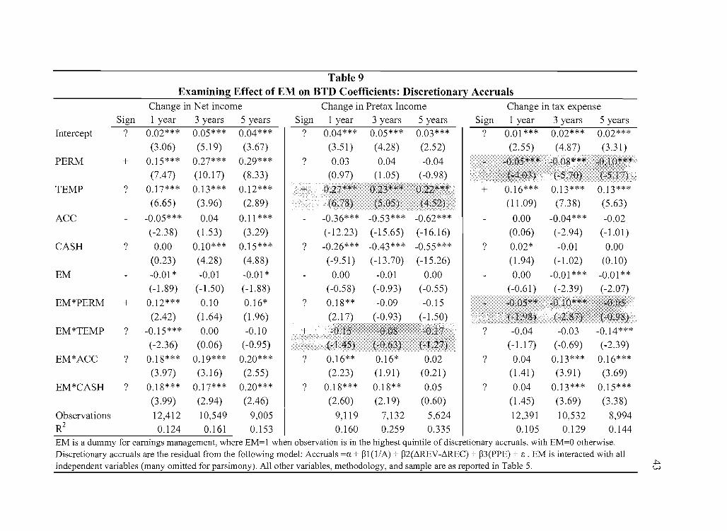
Table 9Examining Effect of EM on BTD Coefficients: Discretionary Accruals

Change in Net income Change in Pretax Income Change in tax expenseSign 1 year 3 years 5 years Sign 1 year 3 years 5 years Sign 1 year 3 years 5 years

Intercept ? 0.02*** 0.05*** 0.04*** ? 0.04*** 0.05*** 0.03*** ? 0.01 *** 0.02*** 0.02***(3.06) (5.19) (3.67) (3.51 ) (4.28) (2.52) (2.55) (4.87) (3.31 )

PERM + 0.15*** 0.27*** 0.29*** ? 0.03 0.04 -0.04(7.47) (10.17) (8.33) (0.97) (1.05) (-0.98)

TEMP ? 0.17*** 0.13*** 0.12*** + 0.16*** 0.13*** 0.13***(6.65) (3.96) (2.89) (11.09) (7.38) (5.63)

ACC - -0.05*** 0.04 0.11 *** - -0.36*** -0.53*** -0.62*** - 0.00 -0.04*** -0.02(-2.38) (1.53) (3.29) (-12.23) (-15.65) (-16.16) (0.06) (-2.94) (-1.01)

CASH ? 0.00 0.10*** 0.15*** ? -0.26*** -0.43*** -0.55*** ? 0.02* -0.01 0.00(0.23) (4.28) (4.88) (-9.51) (-13.70) (-15.26) (1.94) (-1.02) (0.10)

EM - -0.01* -0.01 -0.01 * - 0.00 -0.01 0.00 - 0.00 -0.01 *** -0.01**(-1.89) (-1.50) (-1.88) (-0.58) (-0.93) (-0.55) (-0.61)

EM*PERM + 0.12*** 0.10 0.16* ? 0.18** -0.09 -0.15(2.42) (1.64) (1.96) 1 1

EM*TEMP ? -0.15*** 0.00 -0.10 ? -0.04 -0.03 -0.14***(-2.36) (0.06) (-0.95) (-1.17) (-0.69) (-2.39)

EM*ACC ? 0.18*** 0.19*** 0.20*** ? 0.16** 0.16* 0.02 ? 0.04 0.13*** 0.16***(3.97) (3.16) (2.55) (2.23) (1.91) (0.21) (1.41) (3.91) (3.69)

EM*CASH ? 0.18*** 0.17*** 0.20*** ? 0.18*** 0.18** 0.05 ? 0.04 0.13*** 0.15***(3.99) (2.94) (2.46) (2.60) (2.19) (0.60) (1.45) (3.69) (3.38)

Observations 12,412 10,549 9,005

I9,119 7,132 5,624 12,391 10,532 8,994

R20.124 0.161 0.153 0.160 0.259 0.335 0.105 0.129 0.144

EM is a dummy for earnings management, where EM=1 when observation is in the highest quintile of discretionary accruals, with EM=O otherwise.Discretionary accruals are the residual from the following model: Accruals =a + ~1(1/A) + ~2(f,.REV-f,.REC) + ~3(PPE) + 1;;. EM is interacted with allindependent variables (many omitted for parsimony). All other variables, methodology, and sample are as reported in Table 5. +:0-

w

44

and 6 TAXEXP. Inconsistent with H3b, I find no evidence of a stronger relation between

TEMP and 6PRETAX in the presence of earnings management. However, consistent

with H4b, I now find a negative and significant relation between 6 TAXEXP and the

EM*PERM interaction term for the one year and three periods. This finding suggests that

firms with large, income-increasing discretionary accruals experience an especially large

relation between non-temporary BTDs and future tax expense changes.

Overall, the evidence presented in Tables 6-9 suggests that the relation between

temporary differences and future pretax earnings changes, as well as the relation between

permanent differences and future tax expense changes, are primarily due to underlying

economic events. I find only limited evidence supporting the notion that the

BTD/earnings growth relation is due to earnings management.

45

CHAPTER VII

ROBUSTNESS AND SENSITIVITY TESTS

Reconciliation with Lev and Nissim (2004)

There are several departures in my research design from that employed by Lev and

Nissim (2004). For comparability with their results, I repeat my tests, using their

methodology and sample period.22 There are three key independent variables in their

tests: R_TAX, R_DEF, and R_CFO, which are the quintile rank of the tax to book ratio,

deferred taxes, and cash flows trom operations.23 The tax to book ratio, TAX, is

calculated as the ratio of taxable to book income, where both net income and taxable

income are measured as previously described. DEF is the negative of deferred tax

expense scaled by average total assets. As the ratio of tax to book income, a higher value

of TAX indicates more taxable income, and as the negative of the ratio of deferred tax to

average assets, a higher value ofDEF indicates fewer deferrals and thus greater taxable

income. CFO captures the relative amount of net income coming from cash f1ow, as

opposed to accruals, measured as the difference between net income and accruals, scaled

22 Among the differences between my tests and that of Lev and Nissim (2004) include a shortersample period (their cutoff year is 2000), an inclusion offinns with negative measures of tax expense,computing coefficients and test statistics based on the Fama and MacBeth (1973) methodology ofpresenting the average of the annual coefficients, multiplying dependent variables by 100, and runningranked regressions instead of using the underlying values.

23 Because BTDs can vary across industries due to differences in capital intensity, R&D expenditures(and credits), and other industry-related differences, industry-ranked values of these variables areused, ranking finns each year within their two digit SIC code.

46

by net income. A higher (lower) rank of this variable indicates a greater share of earnings

coming from cash flows (accruals).

Figure 1 presents initial evidence on the relation between BTDs and future

earnings growth. For each measure ofBTD (total differences: R_TAX, and temporary

differences: R_DEF) as well as for the cash flow measure (R_CFO) I form three

portfolios, based on the relative measure of the ranked variable. A continuous line

follows the growth in earnings for firms with the highest quintile of the ratio, a dotted

line for those with intelmediate values, and a dashed line following the growth of

earnings for firms in the lowest quintile. Thus, the solid lines represent growth for firms

with high levels of taxable income in relation to book income, high levels of currently

taxable income in relation to tax-deferred income, and high levels of income from cash

flows in relation to income from accruals. Panel A presents results for growth in total net

income, as in Lev and Nissim (2004).24 Similar to the patterns in their study, I find that

firm-years with relatively high taxable income (high income from cash flows) experience

significantly greater growth in net income compared to firms with relatively lower

taxable income (more income from accruals). There does not appear to be any significant

difference in net income growth for various levels of deferred taxes, the proxy for

temporary BTDs. However, in Panel B, I find evidence that portfolios with higher

taxlbook ratios (high R_TAX) have significantly lower pretax earnings growth than those

with smaller ratios, while the portfolio of high R_DEF finns shows some evidence of

24 Lev and Nissim (2004) present two sets of graphs, pre and post SFAS 109 (1993). However, thepatterns are similar for both periods both in their study and in mine, so for conciseness, I present bothperiods together. The same holds true for multivariate results, where results are similar in bothperiods, so I again present both periods together.

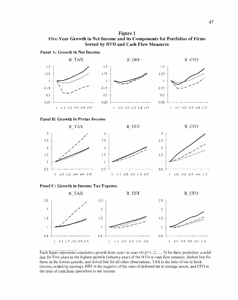
47

Figure 1Five-Year Growth in Net Income and its Components for Portfolios of Firms

Sorted by BTD and Cash Flow Measures

Panel A: Growth in Net Income

R TAX R DEF

1.5

~1.5 1.5

1.25 1.25 1.25

~.-.,~.~.:,>1"""'"

0.75\

0.75 0.75\....,

./'-_./

0.5 0.5 0.5

0.25 0.25 0.25

I 1+1 1+2 1+3 1+4 1+5 I 1+1 1+2 1+3 1+4 1+5

Panel B: Growth in Pretax Income

R CFO

1+ 1 1+2 1+3 1+4 1+5

R TAX R DEF R CFO

3/

2.5 / 2.5//

2

~2

~/ ......

1.5 // ........ 1.5~ ...........

0.5 0.5

1+1 1+2 1+3 1+4 1+5 1+] 1+2 t+3 1+4 1+5

3

2.5

2

1.5

0.5

././

./ .. './ .. '" .

"" ,0'

.~.~ .

t+l t+2 t+3 t+4 t+5

Panel C: Growth in Income Tax Expense

R TAX R DEF R CFO

2.5 2.5/

/2 / 2

//

1.5

~1.5

~/ .'....,,':':':,:,:-0- __

0.5 0.5

I 1+1 1+2 1+3 1+4 1+5 t+l 1+2 1+3 1+4 1+5

2.5

2

1.5

0.5

1+ I 1+2 1+3 t+4 1+5

Each figure represents cumulative growth from year t to year t+j (j=l, 2, ... ,5) for three portfolios: a solidline for firm-years in the highest quintile (industry-year) of the BTD or cash flow measure, dashed line forthose in the lowest quintile, and dotted line for all other observations. TAX is the ratio of tax to bookincome, scaled by earnings, DEF is the negative of the ratio ofdeferred tax to average assets, and CFO isthe ratio of cash from operations to net income.

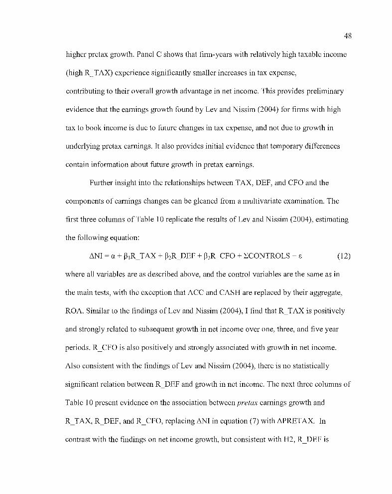
48

higher pretax growth. Panel C shows that finn-years with relatively high taxable income

(high R~TAX) experience significantly smaller increases in tax expense,

contributing to their overall growth advantage in net income. This provides preliminary

evidence that the earnings growth found by Lev and Nissim (2004) for finns with high

tax to book income is due to future changes in tax expense, and not due to growth in

underlying pretax earnings. It also provides initial evidence that temporary differences

contain information about future growth in pretax earnings.

Further insight into the relationships between TAX, DEF, and CFO and the

components of earnings changes can be gleaned from a multivariate examination. The

first three columns of Table 10 replicate the results of Lev and Nissim (2004), estimating

the following equation:

(12)

where all variables are as described above, and the control variables are the same as in

the main tests, with the exception that ACC and CASH are replaced by their aggregate,

ROA. Similar to the findings of Lev and Nissim (2004), I find that R_TAX is positively

and strongly related to subsequent growth in net income over one, three, and five year

periods. R_CFO is also positively and strongly associated with growth in net income.

Also consistent with the findings of Lev and Nissim (2004), there is no statistically

significant relation between R_DEF and growth in net income. The next three columns of

Table 10 present evidence on the association between pretax earnings growth and

R_TAX, R_DEF, and R_CFO, replacing ~NI in equation (7) with ~PRETAX. In

contrast with the findings on net income growth, but consistent with H2, R_DEF is

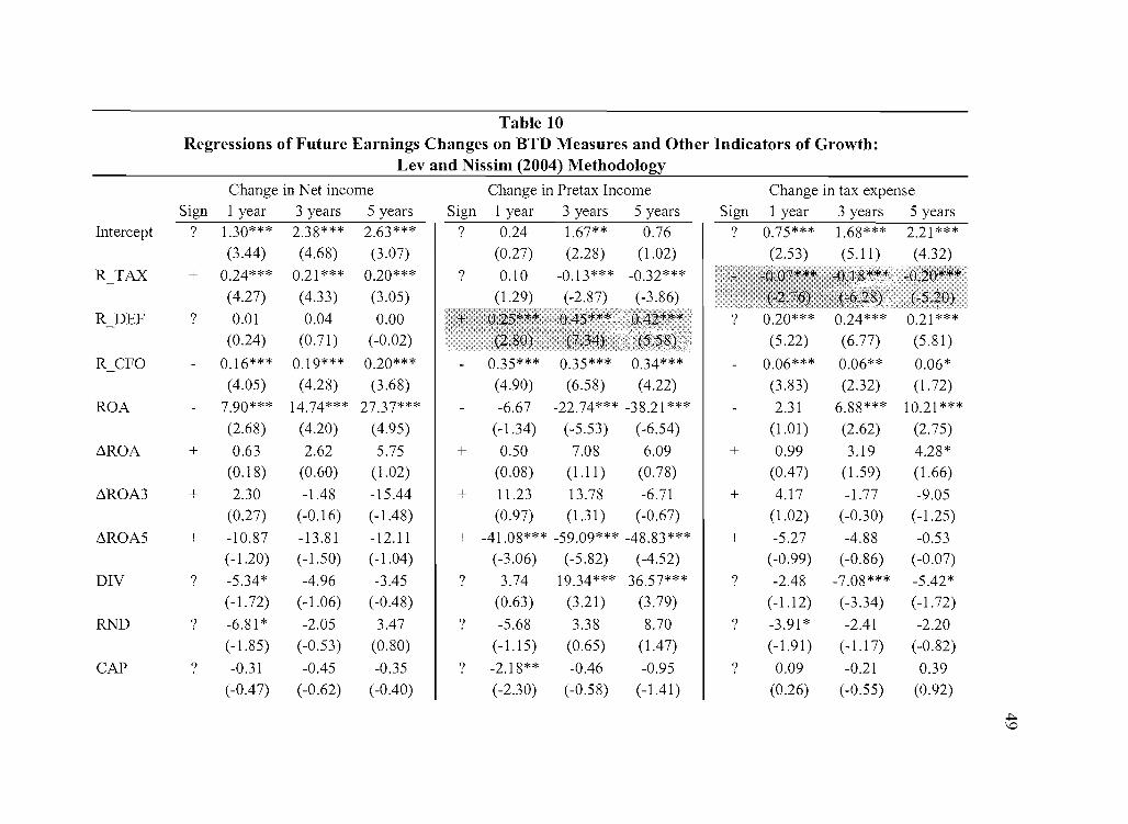
Table 10Regressions of Future Earnings Changes on BTD Measures and Other Indicators of Growth:

Lev and Nissim (2004) Methodology

Change in Net income Change in Pretax Income Change in tax expenseSign 1 year 3 years 5 years Sign 1 year 3 years 5 years Sign 1 year 3 years 5 years

Intercept ? 1.30*** 2.38*** 2.63*** ? 0.24 1.67** 0.76

I? 0.75*** 1.68*** 2.21 ***

(3.44) (4.68) (3.07) (0.27) (2.28) (1.02) (2.53) (5.11 ) (4.32)

R TAX + 0.24*** 0.21 *** 0.20*** ? 0.10 -0.13*** -0.32***(4.27) (4.33) (3.05) (1.29)

R DEF ? 0.01 0.04 0.00(0.24) (0.71) (-0.02) (5.22) (6.77) (5.81)

R CFO - 0.16*** 0.19*** 0.20*** - 0.35*** 0.35*** 0.34*** - 0.06*** 0.06** 0.06*(4.05) (4.28) (3.68) (4.90) (6.58) (4.22) (3.83) (2.32) (1.72)

ROA - 7.90*** 14.74*** 27.37*** - -6.67 -22.74*** -38.21 *** - 2.31 6.88*** 10.21 ***(2.68) (4.20) (4.95) (-1.34) (-5.53) (-6.54) (1.01 ) (2.62) (2.75)

LiROA + 0.63 2.62 5.75 + 0.50 7.08 6.09 + 0.99 3.19 4.28*(0.18) (0.60) (1.02) (0.08) (1.11) (0.78) (0.47) (1.59) (1.66)

LiROA3 + 2.30 -1.48 -15.44 + 11.23 13.78 -6.71 + 4.17 -1.77 -9.05(0.27) (-0.16) (-1.48) (0.97) (1.31) (-0.67) (1.02) (-0.30) (-1.25)

LiROA5 + -10.87 -13.81 -12.11 + -41.08*** -59.09*** -48.83*** + -5.27 -4.88 -0.53(-1.20) (-1.50) (-1.04) (-3.06) (-5.82) (-4.52) (-0.99) (-0.86) (-0.07)

DIV ? -5.34* -4.96 -3.45 ? 3.74 19.34*** 36.57*** ? -2.48 -7.08*** -5.42*(-1.72) (-1.06) (-0.48) (0.63) (3.21 ) (3.79) (-1.12) (-3.34) (-1.72)

RND ? -6.81 * -2.05 3.47 ? -5.68 3.38 8.70 ? -3.91 * -2.41 -2.20(-1.85) (-0.53) (0.80) (-1.15) (0.65) (1.47) (-1.91) (-1.17) (-0.82)

CAP ? -0.31 -0.45 -0.35 ? -2.18** -0.46 -0.95 ? 0.09 -0.21 0.39(-0.47) (-0.62) (-0.40) (-2.30) (-0.58) (-1.41) (0.26) (-0.55) (0.92)

.j:::.\0

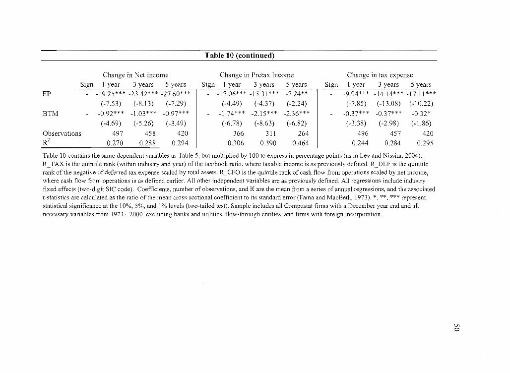
Table 10 (continued)

Change in Net income Change in Pretax Income Change in tax expenseSign 1 year 3 years 5 years Sign 1 year 3 years 5 years Sign 1 year 3 years 5 years

EP - -19.25*** -23.42*** -27.60*** - -17.06*** -15.31 *** -7.24** - -9.94*** -14.14*** -17.11 ***(-7.53) (-8.13) (-7.29) (-4.49) (-4.37) (-2.24) (-7.85) (-13.08) (-10.22)

BTM - -0.92*** -1.03*** -0.97*** - -1.74*** -2.15*** -2.36*** - -0.37*** -0.37*** -0.32*(-4.69) (-5.26) (-3.49) (-6.78) (-8.63) (-6.82) (-3.38) (-2.98) (-1.86)

Observations 497 458 420 366 311 264 496 457 420R2

0.270 0.288 0.294 0.306 0.390 0.464 0.244 0.284 0.295

Table 10 contains the same dependent variables as Table 5, but multiplied by 100 to express in percentage points (as in Lev and Nissim, 2004).R_TAX is the quintile rank (within industry and year) of the tax/book ratio, where taxable income is as previously defined. R_DEF is the quintilerank of the negative of deferred tax expense scaled by total assets. R_CFO is the quintile rank of cash flow from operations scaled by net income,where cash flow from operations is as defined earlier. All other independent variables are as previously defined. All regressions include industryfixed effects (two-digit SIC code). Coefficients, number of observations, and ~ are the mean from a series of annual regressions, and the associatedt-statistics are calculated as the ratio of the mean cross-sectional coefficient to its standard error (Fama and MacBeth, 1973). *, **, *** representstatistical significance at the 10%., 5%" and 1% levels (two-tailed test). Sample includes all Compustat firms with a December year end and allnecessary variables from 1973 - 2000, excluding banks and utilities, flow-through entities, and firms with foreign incorporation.

Vlo

51

positively associated with pretax earnings growth, while R_TAX has either no statistical

association with pretax earnings changes or has a significant negative association. The

final three columns of Table 10 examine the association between R_TAX, R_DEF, and

R CFO with changes in tax expense, replacing L1NI in equation (7) with L1TAXEXP.

Consistent with HI, R_TAX is negatively and strongly associated with changes in tax

expense. These results suggest that the positive relation Lev and Nissim (2004) find

between the tax to book ratio and earnings growth is due to changes in tax expense, not

changes in underlying pretax earnings. Interestingly, there is a positive and significant

relation between R_DEF and L1TAXEXP, indicating higher tax expense changes for firms

with large temporary BTDs. This increase in tax expense is set against the increase in

pretax income for large DEF firms, and the two together may explain why there is no

significant relation between R_DEF and changes in net income.

Firm Fixed Effects

The results presented in Table 5 are based on cross sectional regressions of a

multi-year, multi-firm panel, with both year and industry fixed effects. Because some of

the relations I predict between the BTD components and the components of earnings

changes are mechanical in nature, it could be argued that a time series regression is more

appropriate. To test this, I replace the industry fixed effects with firm fixed effects and

. rerun equations (5), (6), and (7). Table 11 presents the results. While the basic findings

are unchanged, there are some interesting differences. Most notably, the coefficients and

t-stats for the relation between PERM and L1TAXEXP are significantly more negative,

which is not surprising given the mechanical relationship predicted between these

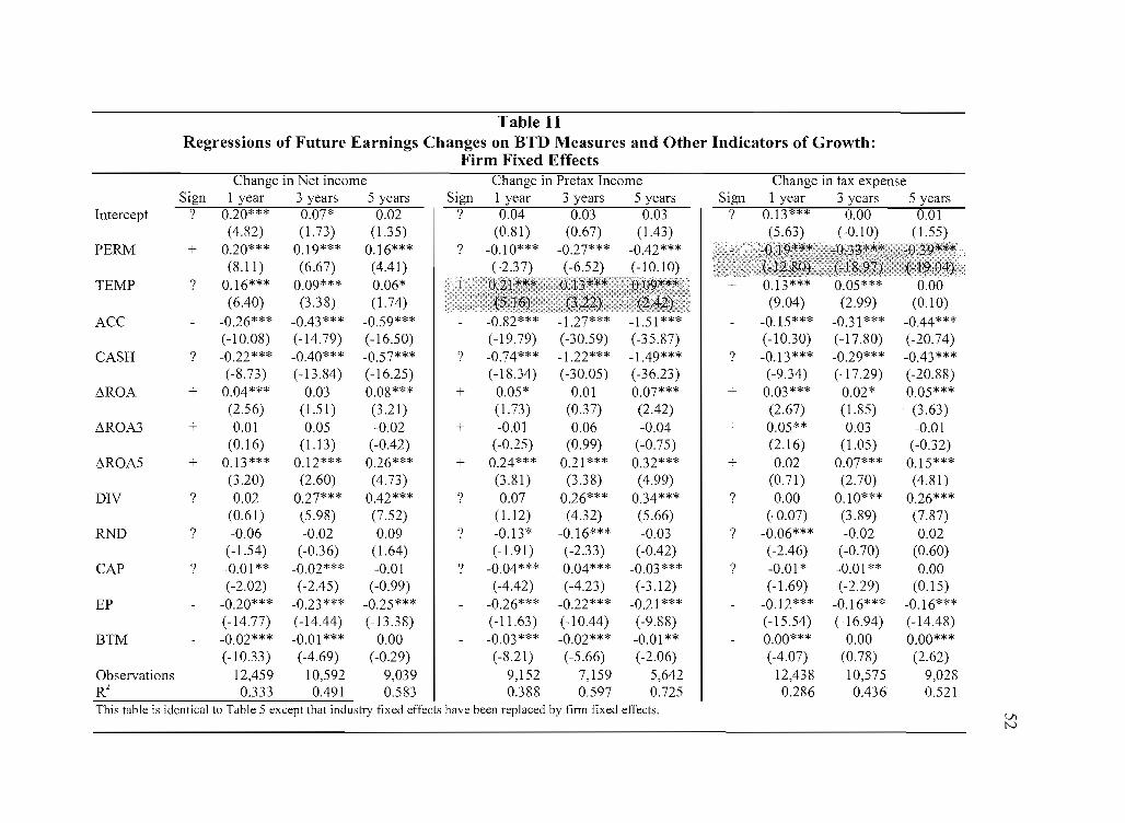
Table 11Regressions of Future Earnings Changes on BTD Measures and Other Indicators of Growth:

Firm Fixed EffectsChange in Net income Change in Pretax Income Change in tax expense

Sign 1 year 3 years 5 years Sign 1 year 3 years 5 years Sign 1 year 3 years 5 yearsIntercept ? 0.20*** 0.07* 0.02 ? 0.04 0.03 0.03

I? 0.13*** 0.00 0.01

(4.82) (1.73) (1.35) (0.81 ) (0.67) (1.43) (5.63) (-0.10) (1.55)PERM + 0.20*** 0.19*** 0.16*** ? -0.10*** -0.27*** -0.42***

(8.11 ) (6.67) (4.41 ) (-10.10)TEMP ? 0.16*** 0.09*** 0.06* + 0.13*** 0.05*** 0.00

(6.40) (3.38) (1.74) (9.04) (2.99) (0.10)ACC -0.26*** -0.43*** -0.59*** - -0.82*** -1.27*** -1.51*** -0.1 5*** -0.31 *** -0.44***

(-10.08) (-14.79) (-16.50) (-19.79) (-30.59) (-35.87) (-10.30) (-17.80) (-20.74)CASH ? -0.22*** -0.40*** -0.57*** ? -0.74*** -1.22*** -1.49*** ? -0.13*** -0.29*** -0.43***

(-8.73) (-13.84) (-16.25) (-18.34) (-30.05) (-36.23) (-9.34) (-17.29) (-20.88).6.ROA + 0.04*** 0.03 0.08*** + 0.05* 0.01 0.07*** + 0.03*** 0.02* 0.05***

(2.56) (1.51) (3.21 ) (1.73 ) (0.37) (2.42) (2.67) (1.85) (3.63 ).6.ROA3 + 0.01 0.05 -0.02 + -0.01 0.06 -0.04 + 0.05** 0.03 -0.01

(0.16) (1.13) (-0.42) (-0.25) (0.99) (-0.75) (2.16) (1.05) (-0.32).6.ROA5 + 0.13*** 0.12*** 0.26*** + 0.24*** 0.21 *** 0.32*** + 0.02 0.07*** 0.15***

(3.20) (2.60) (4.73) (3.81) (3.38) (4.99) (0.71) (2.70) (4.81 )DIV ? 0.02 0.27*** 0.42*** ? 0.07 0.26*** 0.34*** ? 0.00 0.10*** 0.26***

(0.61) (5.98) (7.52) (1.12) (4.32) (5.66) (-0.07) (3.89) (7.87)RND ? -0.06 -0.02 0.09 ? -0.13* -0.16*** -0.03 ? -0.06*** -0.02 0.02

(-1.54) (-0.36) 0.64) (-1.91) (-2.33) (-0.42) (-2.46) (-0.70) (0.60)CAP ? -0.01** -0.02*** -0.01 ? -0.04*** -0.04*** -0.03*** ? -0.01* -0.01 ** 0.00

(-2.02) (-2.45) (-0.99) (-4.42) (-4.23) (-3.12) (-1.69) (-2.29) (0.15)EP -0.20*** -0.23*** -0.25*** -0.26*** -0.22*** -0.21 *** -0.12*** -0.16*** -0.16***

(-14.77) (-14.44) (-13.38) (-11.63) (-10.44) (-9.88) (-15.54) (-16.94) (-14.48)BTM -0.02*** -0.01*** 0.00 -0.03*** -0.02*** -0.01 ** 0.00*** 0.00 0.00***

(-10.33) (-4.69) (-0.29) (-8.21) (-5.66) (-2.06) (-4.07) (0.78) (2.62)Observations 12,459 10,592 9,039 9,152 7,159 5,642 12,438 10,575 9,028RL 0.333 0.491 0.583 0.388 0.597 0.725 0.286 0.436 0.521This table is identical to Table 5 except that industry fixed effects have been replaced by finn fixed effects.

VIN

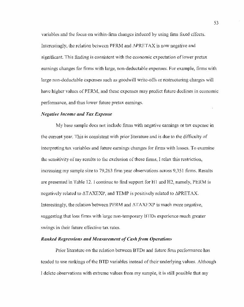
53

variables and the focus on within-finn changes induced by using finn fixed effects.

Interestingly, the relation between PERM and L1PRETAX is now negative and

significant. This finding is consistent with the economic expectation oflower pretax

earnings changes for finns with large, non-deductable expenses. For example, finns with

large non-deductable expenses such as goodwill write-offs or restructuring charges will

have higher values of PERM, and these expenses may predict future declines in economic

perfonnance, and thus lower future pretax earnings.

Negative Income and Tax Expense

My base sample does not include finns with negative earnings or tax expense in

the current year. This is consistent with prior literature and is due to the difficulty of

interpreting tax variables and future earnings changes for finns with losses. To examine

the sensitivity of my results to the exclusion of these finns, I relax this restriction,

increasing my sample size to 79,263 finn year observations across 9,351 finns. Results

are presented in Table 12. I continue to find support for HI and H2, namely, PERM is

negatively related to L1TAXEXP, and TEMP is positively related to L1PRETAX.

Interestingly, the relation between PERM and L1TAXEXP is much more negative,

suggesting that loss finns with large non-temporary BTDs experience much greater

swings in their future effective tax rates.

Ranked Regressions and Measurement of Cash from Operations

Prior literature on the relation between BTDs and future finn perfonnance has

tended to use rankings of the BTD variables instead oftheir underlying values. Although

I delete observations with extreme values from my sample, it is still possible that my

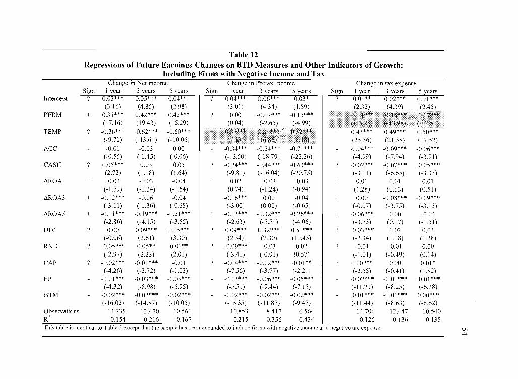
Table 12Regressions of Future Earnings Changes on BTD Measures and Other Indicators of Growth:

Including Firms with Negative Income and TaxChange in Net income Change in Pretax Income Change in tax expense

Sign 1 year 3 years 5 years Sign 1 year 3 years 5 years Sign 1 year 3 years 5 yearsIntercept ? 0.03*** 0.05*** 0.04*** ? 0.04*** 0.06*** 0.03*

I? 0.01** 0.02*** 0.01 ***

(3.16) (4.85) (2.98) (3.01) (4.34) (1.89) (2.32) (4.39) (2.45)PERM + 0.31 *** 0.42*** 0.42*** ? 0.00 -0.07*** -0.15***

(17.16) (19.43) (15.29)TEMP ? -0.36*** -0.62*** -0.60*** + 0.43*** 0.49*** 0.50***

(-9.71) (-13.61) (-10.06) (25.56) (21.38) (17.52)ACC -0.01 -0.03 0.00 -0.34*** -0.54*** -0.71 *** - -0.04*** -0.09*** -0.06***

(-0.55) (-1.45) (-0.06) (-13.50) (-18.79) (-22.26) (-4.99) (-7.94) (-3.91)CASH ? 0.05*** 0.03 0.05 ? -0.24*** -0.44*** -0.63*** ? -0.02*** -0.07*** -0.05***

(2.72) (1.18) (1.64) (-9.81) (-16.04) (-20.75) (-3.11) (-6.65) (-3.33)L'.ROA + -0.03 -0.03 -0.04 + 0.02 -0.03 -0.03 + 0.01 0.01 0.01

(-1.59) (-1.34) (-1.64) (0.74) (-1.24) (-0.94) (1.28) (0.63) (0.51)L'.ROA3 + -0.12*** -0.06 -0.04 + -0.16*** 0.00 -0.04 + 0.00 -0.08*** -0.09***

(-3.11) (-1.36) (-0.68) (-3.00) (0.00) (-0.65) (-0.07) (-3.75) (-3.13)L'.ROA5 + -0.11 *** -0.19*** -0.21 *** + -0.13*** -0.32*** -0.26*** + -0.06*** 0.00 -0.04

(-2.86) (-4.15) (-3.55) (-2.63) (-5.59) (-4.06) (-3.73) (0.17) (-1.51)DIV ? 0.00 0.09*** 0.15*** ? 0.09*** 0.32*** 0.51 *** ? -0.03*** 0.02 0.03

(-0.06) (2.61 ) (3.30) (2.34) (7.30) (10.45) (-2.34) (1.18) (1.28)RND ? -0.05*** 0.05** 0.06** ? -0.09*** -0.03 0.02 ? -0.01 -0.01 0.00

(-2.97) (2.23) (2.01) H.41) (-0.91) (0.57) (-1.01) (-0.49) (0.14)CAP ? -0.02*** -0.01*** -0.01 ? -0.04*** -0.02*** -0.01** ? 0.00*** 0.00 0.01 *

(-4.26) (-2.72) (-1.03) (-7.56) (-3.77) (-2.21) (-2.55) (-0.41) (1.82)EP -0.01 *** -0.03*** -0.03*** -0.03*** -0.06*** -0.05*** -0.02*** -0.01*** -0.01 ***

(-4.32) (-8.98) (-5.95) (-5.51) (-9.44) (-7.15) (-11.21) (-8.25) (-6.28)BTM - -0.02*** -0.02*** -0.02*** -0.02*** -0.02*** -0.02*** -0.01 *** -0.01 *** 0.00***

(-16.02) (-14.87) (-10.05) (-15.35) (-11.87) (-9.47) (-11.44) (-8.63) (-6.62)Observations 14,735 12,470 10,561 10,853 8,417 6,564 14,706 12,447 10,540RL 0.154 0.216 0.167 0.215 0.356 0.434 0.126 0.136 0.138This table is identical to Table 5 except that the sample has been expanded to include finns with negative income and negative tax expense. Vl

..j::,..

55

findings are partially due to exceptionally large or small values of PERM and TEMP, or

to a skewed distribution ofthese variables. To test the sensitivity of my finding to this

possibility, I repeat my tests using the quintile rankings of PERM, TEMP, ACC, and

CASH, and present the results in Table 13.25 There are no meaningful differences from

the previous tests. Another concern is the calculation of the ACC and CASH variables.

ACC are total accruals, based upon the Balance Sheet, and CASH, cash flows from

operations, is the difference between net income and ACC. As a robustness check, I use

the measure of CASH from the Statement of Cash Flows (Compustat #308), and estimate

ACC as the difference between net income and CASH. Since data on the Statement of

Cash Flows is only generally available since 1988, I rerun my main tests using a

restricted sample beginning in 1988, and compare this with tests using the variables based

on the Statement of Cash Flows. Results (untabulated) find no significant change to my

findings using the alternative measures of cash flows and accruals.

Absolute Values

Prior literature has suggested that a possible reason why BTDs predict earnings

changes is that taxable income is a more reliable indicator of firm performance, and that

the farther book income ventures away from this 'true' measure, the lower the quality of

earnings. If this is true, it suggests that the sign of the BTD does not matter, only the

magnitude ofthe difference. To explore this, I rerun my tests using the absolute values of

PERM and TEMP. Results are presented in Table 14. While there appears to be a positive

relation between PERM and changes in tax expense (which results in net income

25As in Lev and Nissim (2004), dependent variables are multiplied by 100 to express in percentagepoints, as the coefficients on ranked variables are very small for presentation purposes otherwise.

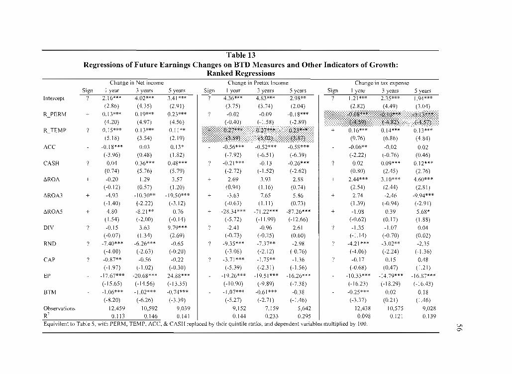
Table 13Regressions of Future Earnings Changes on BTD Measures and Other Indicators of Growth:

Ranked RegressionsChange in Net income Change in Pretax Income Change in tax expense

Sign 1 year 3 years 5 years Sign I year 3 years 5 years Sign I year 3 years 5 yearsIntercept ? 2.16*** 4.02*** 3.41 *** ? 4.36*** 4.83*** 2.98**

I? 1.21 *** 2.35*** 1.94***

(2.86) (4.35) (2.91 ) (3.75) (3.74) (2.04) (4.49) (3.04)

R PERM + 0.13*** 0.19*** 0.23*** ? -0.02 -O'(l9 -0.18***(4.20) (4.97) (4.56) (-0.40) (-1.58)

R TEMP ? 0.15*** 0.13*** 0.11 **(5.18) (3.54) (2.19) (9.76) (6.86) (4.84)

ACC -0.18*** 0.03 0.13* -0.56*** -0.52*** -0.58*** -0.06** -0.02 0.02(-3.96) (0.48) (1.82) (-7.92) (-6.51 ) (-6.39) (-2.22) (-0.76) (0.46)

CASH ? 0.04 0.36*** 0.48*** ? -0.21 *** -0.13 -0.26*** ? 0.02 0.09*** 0.12***(0.74) (5.76) (5.79) (-2.72) (-1.52) (-2.62) (0.80) (2.45) (2.76)

~ROA + -0.20 1.29 3.57 + 2.69 3.93 2.88 + 2.44*** 3.10*** 4.60***(-0.12) (0.57) (1.20) (0.94) (1.16) (0.74) (2.54) (2.44) (2.81 )

~ROA3 + -4.93 -10.30** -19.50*** + -3.63 7.65 5.86 + 2.74 -2.46 -9.94***(-1.40) (-2.22) (-3.12) (-0.63 ) ( 1.11) (0.73) (1.39) (-0.94) (-2.91)

~ROA5 + 4.80 -8.21 ** -0.76 + -28.34*** -71.22*** -87.26*** + -1.08 0.39 5.68*(1.54) (-2.00) (-0.14) (-5.72) (-11.99) (-12.66) (-0.62) (0.17) (1.88)

DIV ? -0.15 3.63 9.79*** ? -2.41 -0.96 2.61 ? -1.35 -1.07 0.04(-0.07) (1.34) (2.69) (-0.73) (-0.25) (0.60) (-1.14) (-0.70) (0.02)

RND ? -7.40*** -6.26*** -0.65 ? -9.35*** -7.37** -2.98 ? -4.21 *** -3.02** -2.35(-4.00) (-2.63 ) (-0.20) (-3.08) (-2.12) (-0.76) (-4.06) (-2.24) (-1.36)

CAP ? -0.87** -0.56 -0.22 ? -3.71 *** -1.75** -1.36 'I -0.17 0.15 0.48(-1.97) (-1.02) (-0.30) (-5.39) (-2.31) (-1.56) (-0.68) (0.47) (1.21)

EP -17.67*** -20.68*** -24.88*** -19.26*** -19.51 *** -16.26*** -10.33*** -14.79*** -16.87***

(-15.65) (-14.56) (-13.35) (-10.90) (-9.89) (-7.38) (-16.23) (-18.29) (-16.43)

BTM -1.06*** -1.02*** -0.74*** -1.07*** -0.61 *** -0.38 -0.25*** 0.02 0.18

(-8.20) (-6.26) (-3.39) (-5.27) (-2.71) (-1.46) (-3.37) (0.21 ) (1.46)

Observations 12,459 10,592 9,039 9,152 7,159 5,642 12,438 10,575 9,028

R20.113 0.146 0.141 0.144 0.233 0.295 0.098 0.121 0.139

Equivilent to Table 5, with PERM, TEMP, ACC, & CASH replaced by their quintile ranks, and dependent variables multiplied by 100. V>.0\

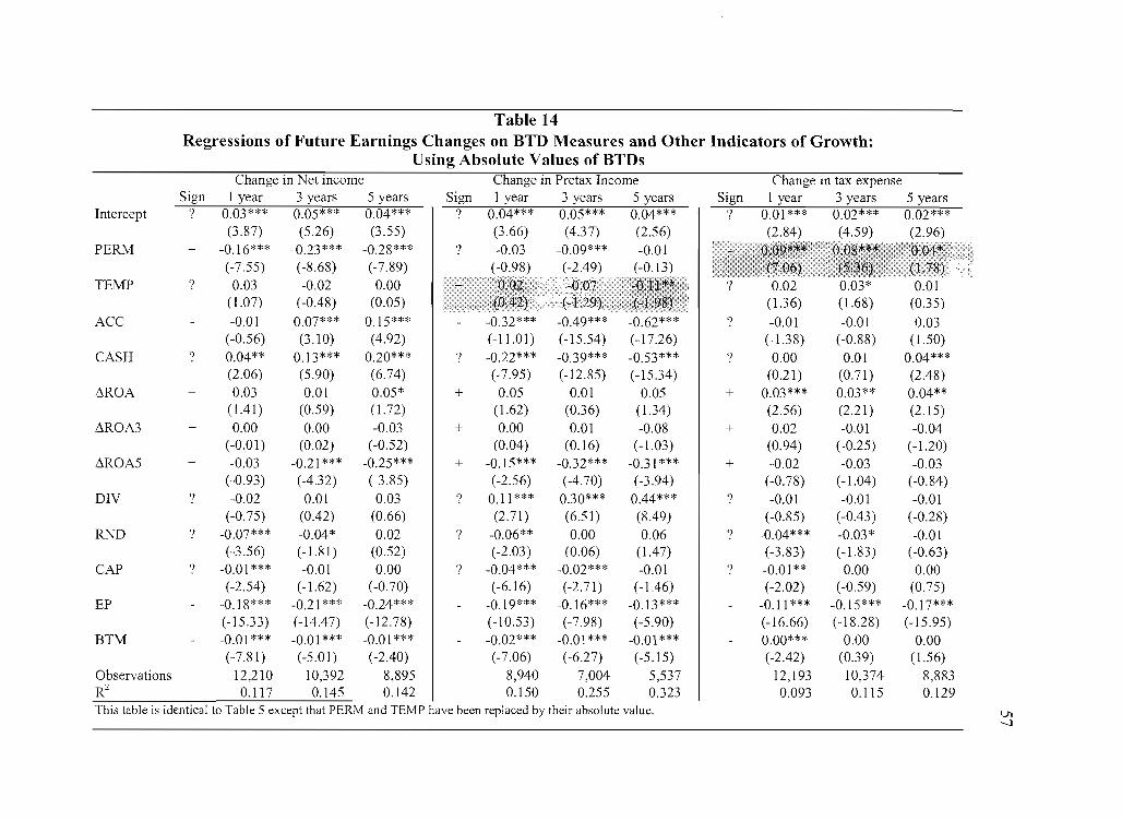
Table 14Regressions of Future Earnings Changes on BTD Measures and Other Indicators of Growth:

Using Absolute Values of BTDsChange in Net income Change in Pretax Income Change in tax expense

Sign 1 year 3 years 5 years Sign 1 year 3 years 5 years Sign 1 year 3 years 5 yearsIntercept '? 0.03*** 0.05*** 0.04*** '? 0.04*** 0.05*** 0.04***

I'? 0.01 *** 0.02*** 0.02***

(3.87) (5.26) (3.55) (3.66) (4.37) (2.56) (2.84) (4.59) (2.96)PERM + -0.16*** -0.23*** -0.28*** ? -0.03 -0.09*** -0.01

(-7.55) (-8.68) (-7.89) (-2.49)TEMP '? 0.03 -0.02 0.00 '? 0.02 0.03* 0.01

(1.07) (-0.48) (0.05) (1.36) (1.68) (0.35)

ACC -0.01 0.07*** 0.15*** -0.32*** -0.49*** -0.62*** '? -0.01 -0.01 0.03(-0.56) (3.10) (4.92) (-11.01) (-15.54) (-17.26) (-1.38) (-0.88) (1.50)

CASH '? 0.04** 0.13*** 0.20*** '? -0.22*** -0.39*** -0.53*** '? 0.00 0.01 0.04***(2.06) (5.90) (6.74) (-7.95) (-12.85) (-15.34) (0.21 ) (0.71) (2.48)

6ROA + 0.03 0.01 0.05* + 0.05 0.01 0.05 + 0.03*** 0.03** 0.04**(1.41 ) (0.59) (1.72) (1.62) (0.36) (1.34) (2.56) (2.21 ) (2.15)

6ROA3 + 0.00 0.00 -0.03 + 0.00 0.01 -0.08 + 0.02 -0.01 -0.04(-0.01 ) (0.02) (-0.52) (0.04) (0.16) (-1.03) (0.94) (-0.25) (-1.20)

6ROA5 + -0.03 -0.21 *** -0.25*** + -0.15*** -0.32*** -0.31 *** + -0.02 -0.03 -0.03(-0.93) (-4.32) (-3.85) (-2.56) (-4.70) (-3.94) (-0.78) (-1.04) (-0.84)

DIV '? -0.02 0.01 0.03 '? 0.11*** 0.30*** 0.44*** '? -0.01 -0.01 -0.01(-0.75) (0.42) (0.66) (2.71 ) (6.51 ) (8.49) (-0.85) (-0.43) (-0.28)

RND '? -0.07*** -0.04* 0.02 ? -0.06** 0.00 0.06 ? -0.04*** -0.03* -0.01(-3.56) (-1.81) (0.52) (-2.03) (0.06) (1.47) (-3.83) (-1.83) (-0.63)

CAP ? -0.01 *** -0.01 0.00 ? -0.04*** -0.02*** -0.01 ? -0.01 ** 0.00 0.00(-2.54) (-1.62) (-0.70) (-6.16) (-2.71) (-1.46) (-2.02) (-0.59) (0.75)

EP -0.18*** -0.21 *** -0.24*** -0.19*** -0.16*** -0.13*** -0.11 *** -0.15*** -0.17***(-15.33) (-14.47) (-12.78) (-10.53) (-7.98) (-5.90) (-16.66) (-18.28) (-15.95)

BTM -0.01 *** -0.01 *** -0.01 *** -0.02*** -0.01 *** -0.01 *** 0.00*** 0.00 0.00(-7.81) (-5.01) (-2.40) (-7.06) (-6.27) (-5.15) (-2.42) (0.39) (1.56)

Observations 12,210 10,392 8,895 8,940 7,004 5,537 12,193 10,374 8,883R" 0.117 0.145 0.142 0.150 0.255 0.323 0.093 0.115 0.129This table is identical to Table 5 except that PERM and TEMP have been replaced by their absolute value. Vl

-.J

58

declines), there is little evidence that the magnitude ofpermanent differences is

associated with future changes in pretax income. There is also no evidence of a relation

between the magnitude of temporary differences and any measure of earnings changes. I

find little support for the notion that the magnitude ofBTDs is associated with future

earnings changes.

Foreign Operations

Throughout this study I find support for HI, that permanent BTDs are negatively

related to future changes in tax expense. I hypothesize this is true because tax accruals

can cause large swings in effective tax rates. A large tax accrual that can generate this

result is PRE, the designation of foreign earnings as pennanently reinvested. To test if

PRE is driving the relation between PERM and ~TAXEXP, I designate a dummy

variable equal to one if a firm has foreign income, and zero otherwise. I then include this

variable in equations (5), (6), and (7) and interact it with each BTD measure as well as

with each control variable. Table 15 presents the results. The negative coefficient on

PERM when examining changes in tax expense suggests that even for finns without

foreign operations there is a negative relation between other tax accruals and tax expense

changes. The negative coefficient on the interaction of the foreign operations dummy

with PERM when examining changes in tax expense suggests that PRE strengthens the

PERM-~TAXEXP relation, in hannony with HI.

Earnings Management

The definitions of earnings management in Tables 6-9 include several choices in

research design. In an attempt to discern the sensitivity ofmy result to design choices, I

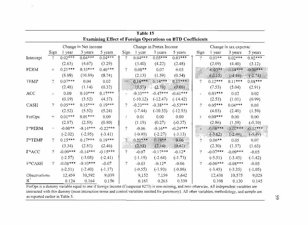
Table 15Examining Effect of Foreign Operations on BTD Coefficients

Change in Net income Change in Pretax Income Change in tax expenseSign 1 year 3 years 5 years Sign I year 3 years 5 years Sign 1 year 3 years 5 years

Intercept ? 0.02*** 0.04*** 0.04*** ? 0.04*** 0.05*** 0.03***

I? 0.01** 0.02*** 0.02***

(2.63) (4.67) (3.29) (3.40) (4.22) (2.48) (2.09) (4.40) (3.12)

PERM + 0.21*** 0.33*** 0.40*** ? 0.08** 0.07 0.03(8.89) (10.89) (9.74) (2.13) (1.59) (0.54)

TEMP ? 0.07*** 0.04 0.02 ? 0.12*** 0.11 *** 0.08***(2.48) (1.14) (0.32) (7.53) (5.04) (2.91)

ACC - 0.00 0.10*** 0.17*** - -0.33*** -0.47*** -0.61 *** - 0.03*** 0.02 0.02(0.19) (3.52) (4.37) (-10.12) (-12.47) (-14.42) (2.53) (1.01) (0.99)

CASH ? 0.05*** 0.15*** 0.19*** ? -0.23*** -0.38*** -0.53*** ? 0.05*** 0.04*** 0.03(2.52) (5.52) (5.24) (-7.44) (-10.33) (-12.93) (4.03) (2.40) (1.59)

ForOps + 0.01 *** 0.01 *** 0.00 + 0.01 0.00 0.00 + 0.00*** 0.00 0.00(2.87) (2.59) (0.80) (1.19) (0.27) (-0.37) 1 (-0.10)

F*PERM + -0.08** -0.14*** -0.22*** ? -0.06 -0.16** -0.24***(-2.02) (-2.95) (-3.41) (-0.99)

F*TEMP ? 0.15*** 0.17*** 0.19*** ? 0.06** 0.05 0.07(3.34) (2.81 ) (2.46) (2.30) (1.37) (1.63)

F*ACC ? -0.09*** -0.14*** -0.15*** ? -0.07 -0.17*** -0.12* ? -0.07*** -0.09*** -0.05(-2.57) (-3.08) (-2.41) (-1.19) (-2.64) (-1.73) (-3.51) (-3.43) (-1.42)

F*CASH ? -0.08*** -0.10*** -0.07 ? -0.03 -0.12* -0.06 ? -0.06*** -0.08*** -0.03(-2.51) (-2.40) (-1.17) (-0.55) (-1.93) (-0.86) (-3.45) (-3.35) (-1.05)

Observations 12,459 10,592 9,039

I9,152 7,159 5,642 12,438 10,575 9,028

R20.124 0.164 0.156 0.161 0.263 0.339 0.108 0.130 0.145

ForOps is a dummy variable equal to one if foreign income (Compustat #273) is non-missing, and zero otherwise. All independent variables areinteracted with this dummy (most interaction tenus and control variables omitted for parsimony). All other variables, methodology, and sample areas reported earlier in Table 5. V1

'-0

60

rerun the tests reported in those tables with the following adjustments (results

untabulated): First, my initial definition of 'narrowly' achieving an earnings target is set

at 0.02. I also use 0.01 and 0.005, with results fundamentally unchanged. Additionally,

prior literature, such as Phillips, Pincus, and Rego (2003), define earnings management as

the contrast between firms that narrowly make an earnings target vs. those that narrowly

miss. As an alternative to the results in Tables 6 and 8, I define the EM dummies in this

way (beat by 0.02 or less vs. miss by .02 or less). Results are substantially unchanged,

although some of the coefficients in support ofH3a and H4a begin to lose their

significance. These results could be due to lack of power, as a significant number of

observations are lost with this narrow definition of earnings management.

61

CHAPTER VIII

CONCLUSION

I examine the relation between book-tax differences and earnings growth. While

prior literature such as Lev and Nissim (2004) find evidence of a relation between total

BTDs and earnings growth, I find evidence consistent with temporary differences

(deferred taxes) being negatively related to growth in pretax earnings, while non­

temporary difference are positively related to earnings growth only because they are

negatively related to tax expense changes. Additionally, I find these results even in the

absence of situations when earnings management is suspected, suggesting that the

relation between BTDs and earnings growth is not a result solely attributable to earnings

management, but that underlying economic events and ETR fluctuations significantly

contribute to the relation. In fact, I find only weak evidence that earnings management

contributes to the relation between temporary BTDs and changes in pretax earnings or the

relation between pennanent BTDs and changes in tax expense.

The findings in this paper contribute to our understanding of how various

measures of BTDs relate to future earnings growth. It answers the call of Graham, Raedy,

and Shackelford (2008) and Hanlon and Heitzman (2009) for investigation into the

components of BTDs. It bridges the conflicting results of two seminal papers on the

relation between BTDs and future perfonnance, as Hanlon (2005) finds a relation

between temporary BTDs and earnings persistence, while Lev and Nissim (2004) find

62

temporary BTDs to be unrelated to future earnings changes. Understanding how

temporary BTDs map into future pretax earnings growth and permanent BTDs map into

future tax expense changes can be a useful distinction for researchers investigating

investor or analyst reaction to BTDs, or when attempting to use BTDs as a measure of

earnings quality.

There are several avenues available for future research. Ayers, Jiang, and

Laplante (2009) find that taxable income is more informative among firms they identify

with 'low earnings quality' and less informative among firms designated as 'tax

planners'. Future work could consider the impact of their measures on the BTD/earnings

growth relation I have documented in this paper. Additionally, many studies examining

the impact BTDs have on market participants define BTDs with the taxlbook ratio.

Because my findings suggest that the different components ofBTDs imply different

things about future economic performance, the breakdown of BTDs into its compon~nts

may reveal how well market participants understand these differences. Finally, the results

on earnings management are somewhat surprising and subject to various limitations.

Future work using more refined measures of earnings management will perhaps yield

results more consistent with the existing literature and the hypotheses developed in this

paper.

63

BIBLIOGRAPHY

Ayers, B., J. Jiang, and S. Laplante. 2009. Taxable income as a performance measure:The effects of tax planning and earnings quality. Forthcoming in ContemporaryAccounting Research.

Bauman, c., M. Bauman, and R. Halsey. 2001. Do firms use the deferred tax assetvaluation allowance to manage earnings? The Journal of the American TaxationAssociation 23 :27-48.

Blouin, J., and 1. Tuna. 2007. Tax Contingencies: Cushioning the blow to earnings?Working paper, University of Pennsylvania.

Burgstahler, D. and 1. Dichev, 1997. "Earnings management to avoid earnings decreasesand losses." Journal ofAccounting and Economics, 24,99-126.

Chan, 1., J. Karceski, and J. Lakonishok. 2003. The level and persistence of growth rates.Journal ofFinance 58: 643-684.

Dechow, P., R. Sloan, and A. Sweeney. 1995. Detecting earnings management. TheAccounting Review: 70,193-225.

Degeorge, F., 1. Patel, and R. Zeckhauser. 1999. Earnings management to exceedthresholds. The Journal ofBusiness, 72,1-33.

Dhaliwal, D., C. Gleason, and L. Mills. 2004. Last chance earnings management: Usingthe tax expense to meet analysts' forecasts. Contemporary Accounting Research21: 431-459.

Dhaliwal, D., R. Huber, H. Lee, and M. Pincus. 2008. Variability of book-tax differences,information uncertainty, and implied cost of capital. Working paper, University ofArizona, UC Irvine.

Dyreng, S., M. Hanlon, and E. Maydew. 2008. Long-run corporate tax avoidance. TheAccounting Review 83:61-82

Fama, E. and K. French. 1992. The cross-section of expected stock returns. Journal ofFinance 47: 427-465.

64

Fama, E. and J. MacBeth. 1973. "Risk return and equilibrium: Empirical tests." Journala.!Political Economy 71 :607-636.

Frank, M.M. and S. Rego. 2006. Do managers use the valuation allowance account tomanage earnings around certain earnings targets? Journal of the AmericanTaxation Association 28: 43-65.

Graham, J., J. Raedy, and D. Shackelford. 2008. Research in accounting for incometaxes. Working paper, Duke University and University of North Carolina.

Gupta, S., and R. Laux. 2008. Do firms use tax cushion reversals to meet earningstargets? Working paper, Michigan State University, Arizona State University.

Hanlon, M. 2003. What can we infer about a firm's taxable income from its financialstatements? National Tax Journal 56: 831-864.

Hanlon, M. 2005. The persistence and pricing of earnings, accruals and cash flows whenfirms have large book-tax differences. The Accounting Review 80:137-166.

Hanlon, M. and S. Heitzman. 2009. Tax research: real effects, earnings management, andgovernance. Working paper, University ofMichigan and University of Rochester.

Hanlon, M. and G. Krishnan. 2006. Do auditors use the infonnation reflected in book-taxdifferences? Working paper, University ofMichigan and George MasonUniversity.

Healy, P. 1985. The effect of bonus schemes on accounting decisions. Journal ofAccounting and Economics 7: 85-107.

Joos, P., J. Pratt, and D. Young. 2000. Book-tax differences and the value relevance ofearnings. Working paper, Massachusetts Institute of Technology, IndianaUniversity, and INSEAD.

Krull, L. 2004. Permanently reinvested foreign earnings, taxes, and earnmgsmanagement. The Accounting Review 79: 745-767.

Lev, B., and D. Nissim. 2004. Taxable income, future earnings, and equity values. TheAccounting Review 79: 1039-1074.

Manzon, G. and G. Plesko. 2002. The relation between financial and tax reportingmeasures of income. The Law Review 55: 175-214.

McGill, G. and E. Outslay. 2002. Did Enron pay taxes? Using accounting information todecipher tax status. Tax Notes (August 19): 1125-1136.

65

Miller, G., and D. Skinner. 1998. Determinants of the valuation allowance for deferredtax assets under SFAS No. 109. The Accounting Review 73: 213-233.

Mills, L. and G. Plesko. 2003. Bridging the reporting gap: A proposal for moreinformative reconciling of book and tax income. National Tax Journal 56: 865­893.

Mills, L. and K. Newberry. 2001. The influence of tax and nontax costs on book-taxreporting differences: Public and private firms. Journal ofthe American TaxAssociation 23: 1-19.

Mills, L., K. Newberry, and W. Trautman, 2002. Trends in book-tax income and balancesheet differences. Tax Notes (August 19): 1109-1124.

Phillips, J., M. Pincus, and S. Rego. 2003. Earnings management: New evidence basedon deferred tax expense. The Accounting Review 78: 491-521.

Schrand, c., and F. Wong. 2003. Earnings management using the valuation allowance fordeferred tax assets under SFAS No.1 09. Contemporary Accounting Research 20:579-611.

Shevlin, T. 2002. Corporate tax shelters and book-tax differences. Tax Law Review55:427-443.

Sloan, R. 1996. Do stock prices fully reflect information in accruals and cash flows aboutfuture earnings? The Accounting Review 71 :289-315.

Tang, T. 2005. Book-tax differences, a proxy for earnings management and taxmanagement - Empirical evidence from China. Working paper, The AustralianNational University.

Visvanathan, G. 1998. Deferred tax valuation allowances and earnings management.Journal ofFinancial Statement Analysis 3:6-1 O.

Weber, D. 2008. Book-tax differences, analysts' forecast errors, and stock returns.Working paper, University of Connecticut.

Weisman, J. 2002. At firms, dual profit pictures: The gap grows between what's earnedand what's taxed. The Washington Post (October 10): AOI.