Embed Size (px)
Citation preview
Combinatorics, Probability and Computing (2004) 13, 577–625. c© 2004 Cambridge University Press
DOI: 10.1017/S0963548304006315 Printed in the United Kingdom
Boltzmann Samplers
for the Random Generation
of Combinatorial Structures
P H I L I P P E D U C H O N,1 P H I L I P P E F L A J O L E T,2
G U Y L O U C H A R D3 and G I L L E S S C H A E F F E R4
1 LaBRI, Universite de Bordeaux I, 351 Cours de la Liberation, F-33405 Talence Cedex, France
(e-mail: [email protected])
2 Algorithms Project, INRIA-Rocquencourt, F-78153 Le Chesnay, France
(e-mail: [email protected])
3 Universite Libre de Bruxelles, Departement d’informatique,
Boulevard du Triomphe, B-1050 Bruxelles, Belgique
(e-mail: [email protected])
4 Laboratoire d’Informatique (LIX), Ecole Polytechnique, 91128 Palaiseau Cedex, France
(e-mail: [email protected])
Received 1 January 2003; revised 31 December 2003
This article proposes a surprisingly simple framework for the random generation of com-
binatorial configurations based on what we call Boltzmann models. The idea is to perform
random generation of possibly complex structured objects by placing an appropriate
measure spread over the whole of a combinatorial class – an object receives a probability
essentially proportional to an exponential of its size. As demonstrated here, the resulting
algorithms based on real-arithmetic operations often operate in linear time. They can be
implemented easily, be analysed mathematically with great precision, and, when suitably
tuned, tend to be very efficient in practice.
1. Introduction
In this study, Boltzmann models are introduced as a framework for the random generation
of structured combinatorial configurations, such as words, trees, permutations, constrained
graphs, and so on. A Boltzmann model relative to a combinatorial class C depends on
a real-valued (continuous) control parameter x > 0 and places an appropriate measure
that is spread over the whole of C. This measure is essentially proportional to x|ω| for an
object ω ∈ C of size |ω|. Random objects under a Boltzmann model then have a fluctuating
size, but objects with the same size invariably occur with the same probability. In particular,
a Boltzmann sampler (i.e., a random generator that produces objects distributed according
578 P. Duchon, P. Flajolet, G. Louchard and G. Schaeffer
Table 1.
Preprocessing memory Preprocessing time Time per generation
O(n) large integers O(n2) or O(n1+ε) O(n log n)
to a Boltzmann model) draws uniformly at random an object of size n, when the size of
its output is conditioned to be the fixed value n.
As we demonstrate, Boltzmann samplers can be derived systematically (and simply) for
classes that are specified in terms of a basic collection of general-purpose combinatorial
constructions. These constructions are precisely the ones that surface recurrently in modern
theories of combinatorial analysis [4, 28, 30, 60, 61] and in systematic approaches to
random generation of combinatorial structures [29, 51]. As a consequence, one obtains with
surprising ease Boltzmann samplers covering an extremely wide range of combinatorial
types.
In most of the combinatorial literature so far, fixed-size generation has been the standard
paradigm for the random generation of combinatorial structures, and a vast literature
exists on the subject. There, either specific bijections are exploited or general combinatorial
decompositions are put to use in order to generate objects at random based on counting
possibilities – the latter approach has come to be known as the ‘recursive method’,
originating with Nijenhuis and Wilf [51], then systematized and extended by Flajolet,
Zimmermann and Van Cutsem in [29]. In contrast, the basic principle of Boltzmann
sampling is to relax the constraint of generating objects of a strictly fixed size, and prefer
to draw objects with a randomly varying size. As we shall see, normally, one can then tune
the value of the control parameter x in order to favour objects of a size in the vicinity
of a target value n. (A ‘tolerance’ of, say, a few per cent on size of the object produced
is likely to cater for many practical simulation needs.) If the tuning mentioned above is
not sufficient, one can always pile up a rejection method to restrict further the size of the
element drawn. In this way, Boltzmann samplers may be employed for approximate-size
as well as fixed-size random generation.
We propose Boltzmann samplers as an attractive alternative to standard combinatorial
generators based on the recursive method and implemented in packages like Combstruct
(under the computer algebra system Maple) and CS (under MuPAD). The algorithms
underlying the recursive method necessitate a preprocessing phase where tables of integer
constants are set up, then they appeal to a boustrophedonic strategy in order to draw a
random object of size n. In the abstract, the integer-arithmetic complexities attached to
the recursive method and measured by the number of (large) integer-arithmetic operations
are as shown in Table 1. The integer-based algorithms require the costly maintenance
of large tables of constants (in number O(n)). In fact, they effect arithmetic operations
over large multiprecision integers, which themselves have size O(n) (in the unlabelled
case) or O(n log n) (in the labelled case); see [29]. Consequently, the overall Boolean
complexities involve an extra factor of O(n) at least, leading to a cost measured in
elementary operations that is quadratic or worse. (The integer-arithmetic time of the
preprocessing phase could in principle be decreased from O(n2) to O(n1+ε) thanks to the
Boltzmann Samplers for Random Generation 579
Table 2.
Preprocessing memory Preprocessing time Time per generation
O(1) real constants ‘small’ ≈ O((log n)k) O(|ω|) [‘free’ gen. of ω]
O(n) [with tolerance]
recent work of van der Hoeven [65], but this does not affect our basic conclusions.) An
alternative, initiated by Denise, Dutour and Zimmermann [12, 13], consists in treating
integers as real numbers and approximating them using real arithmetics (‘floating point’
implementations), possibly supplementing the technique by adaptive precision routines. In
the case of real-based algorithms, the Boolean as well as practical complexities improve,
and they become fairly well represented by the data of Table 1, but the memory and
time costs of the preprocessing phase remain fairly large, while the time per generation
remains inherently superlinear.
As we propose to show, Boltzmann algorithms can well be competitive when compared
to combinatorial methods: Boltzmann samplers only necessitate a small fixed number of
low precision real constants that are normally easy to compute while their complexity is
always linear in the size of the object drawn. Accordingly, uniform random generation
of objects with sizes in the range of millions is becoming a possibility, whenever the
Boltzmann framework is applicable. The price to be paid is an occasional loss of certainty
in the exact size of the object generated, typically, a tolerance on sizes of a few percents
should be granted; see Table 8 in Section 8. Table 2 summarizes the complexities of
Boltzmann generators, measured in real-arithmetic operations. The preprocessing memory
is O(1), meaning that only a fixed number of real-valued constants are needed, once the
control parameter x is fixed. The vague qualifier ‘small’ attached to preprocessing time
refers to the fact that implementations are based on floating point approximations to
exact real number arithmetics, in which case, typically, the preprocessing time is likely to
be a small power of log n. (That this preprocessing is practically feasible and of a very low
complexity should at least transpire from the various examples given, but a systematic
discussion would carry us too far away from our main objectives.1) As regards the time
consumed by random generation per se, it is invariably proportional to the size of the
generated object ω when a Boltzmann sampler operates ‘freely’, equipped with a fixed
value of parameter x: see Theorems 3.1 and 4.1 below. The generation time is O(n) in a
very large number of cases, whenever a tolerance is allowed and sizes in an interval of
the form [n(1 − ε), n(1 + ε)] are accepted: see Theorems 6.1–7.3 for detailed conditions.
As regards random generation, the ideas presented here draw their origins from many
sources. First the recursive method of [29, 51] served as a key conceptual guide for
delineating the types of objects that are systematically amenable to Boltzmann sampling.
Ideas from a statistical physics point of view on combinatorics, of which great use was
made by Vershik and his collaborators [10, 67], then provided crucial insight regarding the
1 The primary goal of this article is practical algorithmic design, not complexity theory, although a fair amount
of analysis, by necessity, enters into the discussion.
580 P. Duchon, P. Flajolet, G. Louchard and G. Schaeffer
new class of algorithms for random generation that is presented here. Another important
ingredient is the collection of rejection algorithms developed by Duchon, Louchard and
Schaeffer for certain types of trees, polyominoes, and planar maps [17, 45, 56]. There
are also similarities to the technique of ‘shifting the mean’ (see Greene and Knuth’s
book [33, pp. 78–80]) as well as the theory of large deviations [11] and ‘exponential
families’ of probability theory – we have benefited from discussions with Alain Denise on
these aspects. Finally, the principles of analytic combinatorics (see [28]) provide essential
clues for deciding situations in which the algorithms are likely to be efficient. Further
connections are discussed at the end of the next section.
Plan of this study. Boltzmann models and samplers are introduced in Section 2. Boltzmann
models exist in two varieties: the ordinary and the exponential models. Ordinary models
serve for combinatorial classes that are ‘unlabelled’, the corresponding samplers being
developed in Section 3, where basic construction rules are described. Section 4 proceeds
in a parallel way with exponential models and ‘labelled’ classes. Some of the complexity
issues raised by Boltzmann sampling are examined in Section 5. There it is shown that,
at least in the idealized sense of exact real-number computations, a Boltzmann sampler
suitably equipped with a fixed (and small) number of driving constants operates in time
that is linear in the (fluctuating) size of the object it produces.
Sections 2 to 5 develop Boltzmann samplers that operate freely under the sole effect
of the defining parameter x. We examine next the way the control parameter x can be
tuned to attain objects at or near a target value: this is the subject of Section 6, where
rejection is introduced and a technique based on the pointing transformation is developed.
Section 7 describes two types of situation where the basic Boltzmann samplers turn out
to be optimized by assigning a critical value to the control parameter x. Section 8 offers
a few concluding remarks.
An extended abstract summarizing several of the results described here has been
presented at the ICALP’2002 Conference in Malaga [18].
2. Boltzmann models and samplers
We consider a class C of combinatorial objects of sorts, with | · | the size function mapping
C to Z0. By Cn is meant the subclass of C comprising all the objects in C having size n,
and each Cn is assumed to be finite. One may think of binary words (with size defined as
length), permutations, graphs and trees of various types (with size defined as number of
vertices), and so on. Any set C endowed with a size function and satisfying the finiteness
axiom will henceforth be called a combinatorial class.
The uniform probability distribution over Cn assigns to each γ ∈ Cn the probability
PCnγ = 1/Cn,
with Cn := card(Cn). Exact-size random generation means the process of drawing uni-
formly at random from the class Cn. We also consider (see Sections 6 and 7 for a
description of various strategies) random generation from ‘neighbouring classes’, CN
where N may not be totally under control, but should still be in the vicinity of n,
Boltzmann Samplers for Random Generation 581
namely, in some interval (1 − ε)n N (1 + ε)n, for some ‘tolerance’ factor ε > 0; this is
called approximate-size (uniform) random generation. It must be stressed that, even under
approximate-size random generation, two objects of the same size are invariably drawn
with the same probability.
Definition. The Boltzmann models of parameter x exist in two varieties, the ordinary
version and the exponential version. They assign to any object γ ∈ C the following
probability:
ordinary/unlabelled case: Px(γ) =1
C(x)· x|γ| with C(x) =
∑γ∈C
x|γ|,
exponential/labelled case: Px(γ) =1
C(x)· x
|γ|
|γ|! with C(x) =∑γ∈C
x|γ|
|γ|! .
A Boltzmann sampler (or generator) ΓC(x) for a class C is a process that produces objects
from C according to the corresponding Boltzmann model, either ordinary or exponential.
The normalization coefficients are nothing but the values at x of the counting generating
functions, respectively of ordinary type (OGF) for C and exponential type (EGF) for C:
C(z) =∑n0
Cnzn, C(z) =
∑n0
Cnzn
n!.
Coherent values of x defined to be such that 0 < x < ρC (or ρC), with ρf the radius of
convergence of f, are to be considered. The quantity ρf is referred to as the ‘critical’ or
‘singular’ value. (In the particular case when the generating function C(x) still converges
at ρC , one may also use the limit value x = ρC to define a valid Boltzmann model; see
Section 7 for uses of this technique.)
For reasons which will become apparent, we have introduced two categories of models,
the ordinary and exponential ones. Exponential Boltzmann models are appropriate for
handling labelled combinatorial structures, while ordinary models correspond to unlabelled
structures of combinatorial theory.2 In the unlabelled universe, all elementary components
of objects (‘atoms’) are indistinguishable, while in the labelled universe, they are all
distinguished from one another by bearing a distinctive mark, say one of the integers
between 1 and n if the object considered has size n. Permutations written as sequences of
distinct integers are typical labelled objects while words over a binary alphabet appear as
typical unlabelled objects made of ‘anonymous’ letters, say a, b for a binary alphabet.
For instance, consider the (unlabelled) class W of all binary words, W = a, b. There
are Wn = 2n words of length n and the OGF is W (z) = (1 − 2z)−1. The probability
assigned by the ordinary Boltzmann model to any word w is x|w|(1 − 2x). There, the
coherent values of x are all the positive values less than the critical value ρW = 12. The
probability that a word of length n is selected is (2x)n(1 − 2x), so that the Boltzmann
2 This terminology is standard in combinatorial enumeration and graph theory; see, e.g., the books of Bergeron,
Labelle and Leroux [4], Goulden and Jackson [30], Harary and Palmer [34], Stanley [60, 61] and Wilf [69]
or the preprints by Flajolet and Sedgewick [28].
582 P. Duchon, P. Flajolet, G. Louchard and G. Schaeffer
model of binary words is logically equivalent to the following process: draw a random
variable N according to the geometric distribution of parameter 2x; if the value N = n is
obtained, draw uniformly at random any of the possible words of size n. For the labelled
case, consider the class K of all cyclic permutations, K = [1], [1 2], [1 2 3], [1, 3, 2], . . . .
There are Kn = (n− 1)! cyclic permutations of size n over the canonical set of ‘labels’
1, . . . , n. The EGF is
K(z) =∑n1
(n− 1)!zn
n!=
∑n1
zn
n= log
1
1 − z. (2.1)
The probability of drawing a cyclic permutation of some fixed size n is then
1
log(1 − x)−1
xn
n, (2.2)
a quantity defined for 0 < x < ρK = 1. (This is known as the ‘logarithmic series distri-
bution’; see Section 4). As in the case of binary words, the Boltzmann model can thus
be realized by first selecting size according to the logarithmic series distribution, and
then by drawing uniformly at random a cyclic permutation of the chosen size. We are
precisely going to revert this process and show that, in many cases, it is of advantage to
draw directly from a Boltzmann model (Sections 3 to 5), and from there derive random
generators that are efficient for a given range of sizes (Sections 6 and 7).
The size of the resulting object under a Boltzmann model is a random variable denoted
throughout by N. By construction, the probability of drawing an object of size n is, under
the model of index x,
Px(N = n) =Cnx
n
C(x), or Px(N = n) =
Cnxn
n!C(x), (2.3)
for the ordinary and exponential model, respectively. The law is well quantified by the
following lemma. (See, e.g., Huang’s book [37] for similar calculations from the statistical
mechanics angle.)
Proposition 2.1. The random size of the object produced under the ordinary Boltzmann
model of parameter x has first and second moments satisfying
Ex(N) = xC ′(x)
C(x), Ex(N
2) =x2C ′′(x) + xC ′(x)
C(x). (2.4)
The same expressions are valid, but with C replacing C , in the case of the exponential
Boltzmann model. In both cases, the expected size Ex(N) is an increasing function of x.
Proof. Under the ordinary Boltzmann model, the probability generating function of N is∑n
Px(N = n)zn =C(xz)
C(x),
by virtue of (2.3). The result then immediately follows by differentiation setting z = 1:
Ex(N) =
(∂
∂z
C(xz)
C(x)
)z=1
, Ex(N(N − 1)) =
(∂2
∂z2
C(xz)
C(x)
)z=1
.
Boltzmann Samplers for Random Generation 583
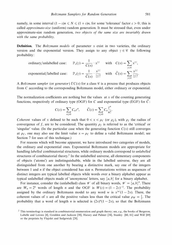
Figure 1. Size distributions under Boltzmann models for various values of parameter x. From top to bottom: the
‘bumpy’ type of set partitions (Example 5), the ‘flat’ type of surjections (Example 6), and the ‘peaked’ type of
general trees (Example 2)
The very same calculation applies to exponential Boltzmann models, but with the EGF
C then replacing the OGF C .
The mean size Ex(N) is always a strictly increasing function of x as soon as the class Ccontains at least two elements of different sizes. Indeed, by a trite calculation we verify
the identity
xd
dxEx(N) = Vx(N),
where V denotes the variance operator. Since the variance of a nondegenerate random
variable is always strictly positive, the derivative of Ex(N) is positive and Ex(N) is in-
creasing. (This property is in fact a special case of Hadamard’s convexity theorem.)
For instance, in the case of binary words, the coherent choice x = 0.4 leads to a size
with mean value 4 and standard deviation about 4.47; for x = 0.49505, the mean and
standard deviation of size become respectively 100 and 100.5. For cyclic permutations,
we determine similarly that the choice x = 0.99846 leads to an object of mean size equal
to 100, while the standard deviation is somewhat higher than for words, being equal to
234. In general, the distribution of random sizes under a Boltzmann model, as given by
(2.3), strongly depends on the family under consideration. Figure 1 illustrates three widely
differing profiles: for set partitions, the distribution is ‘bumpy’, so that a choice of the
appropriate x will most likely generate an object close to the desired size; for surjections
584 P. Duchon, P. Flajolet, G. Louchard and G. Schaeffer
(whose behaviour is analogous to that of binary words), the distribution becomes fairly
‘flat’ as x nears the critical value; for trees, it is ‘peaked’ at the origin, so that very small
objects are generated with high probability. It is precisely the purpose of later sections
(Sections 6 and 7) to recognize and exploit the ‘physics’ of these distributions in order to
deduce efficient samplers for exact and approximate size random generation.
Relation to other fields. The term ‘Boltzmann model’ comes from the great statistical
physicist Ludwig Boltzmann, whose works (together with those of Gibbs and Maxwell)
led to the following principle: Statistical mechanical configurations of energy equal to E in
a system have a probability3 of occurrence proportional to e−βE . If one identifies size of a
combinatorial configuration with energy of a thermodynamical system and sets x = e−β ,
then what we term the ordinary Boltzmann models become the usual model of statistical
mechanics. The counting generating function in the combinatorial world then coincides
with the normalization constant in the statistical mechanics world, where it is known
as the partition function – the Zustandsumme, often denoted by Z . (Note: In statistical
mechanics, β = 1/(kT ) is an inverse temperature. Thus situations where x → 0 formally
correspond to low temperatures or ‘freezing’ and give more weight to small structures,
while x → ρ− corresponds to high temperatures or ‘melting’, that is, to larger sizes of the
combinatorial configurations being generated.)
Exponential weights of the Boltzmann type are naturally essential to the simulated
annealing approach to combinatorial optimization. In the latter area, for instance, Fill
and Huber [22] have shown the possibility of drawing at random independent sets of
graphs according to a Boltzmann distribution, at least for certain values of the control
parameter x = e−β . Closer to us, Compton [7, 8] has made an implicit use of what we call
Boltzmann models for the analysis of 0–1 laws and limit laws in logic; see also the account
by Burris [6]. Vershik has initiated in a series of papers (see [67] and references therein)
a programme that can be described in our terms as first developing the probabilistic
study of combinatorial objects under a Boltzmann model and then ‘returning’ to fixed
size statistics by means of Tauberian arguments of sorts. (A similar description can be
applied to Compton’s approach; see especially the work of Milenkovic and Compton [50]
for recent developments in this direction.) As these examples indicate, the general idea of
Boltzmann models is certainly not new, and, in this work, we may at best claim originality
for aspects related to the fast random generation of combinatorial structures.
3. Ordinary Boltzmann generators
In this section and the next one, we develop a collection of rules by which one can
assemble Boltzmann generators from simpler ones. The combinatorial classes considered
are built by means of a small set of constructions that have wide expressive power. The
3 Distributions of the type e−βE play an important role in the study of point processes and they tend to be
known to probabilists under the name of ‘Gibbs measures’.
Boltzmann Samplers for Random Generation 585
language in which classes are specified is in essence the same as the one underlying the
recursive method [29]: it includes the constructions of union, product, sequence, and, in
the labelled case treated in the next section, the additional set and cycle constructions.
For each allowable class, a Boltzmann sampler can be derived in an entirely systematic
(and even automatic) manner.
A combinatorial construction builds a new class C from structurally simpler classes
A,B, in such a way that Cn is determined from smaller objects, that is, from elements
of Ajnj=0, Bjnj=0. The unlabelled constructions considered here are disjoint union
(+), Cartesian product (×), and sequence formation (S). We define these in turn and
concurrently build the corresponding Boltzmann sampler ΓC for the composite class C,
given random generators ΓA,ΓB for the ingredients and assuming the values of intervening
generating functions A(x), B(x) at x to be real numbers which are known exactly.
Finite sets. Clearly if C is finite (and in practice small), one can generate a random
element of C by selecting it according to the finite probability distribution defined by the
Boltzmann model: if F = ω1, . . . , ωr, then one selects fj with probability proportional
to z|fj |. Thus, drawing from a finite set is equivalent to a finite probabilistic switch.
Drawing from a singleton set is then a deterministic procedure which directly outputs the
object in question. In particular, in what follows, we make use of the singleton classes,
1 and Z, formed respectively of one element of size 0 (analogous to the empty word of
formal language theory) and of one element of size 1 that can be viewed as a generic
‘atom’ out of which complex combinatorial structures are formed.
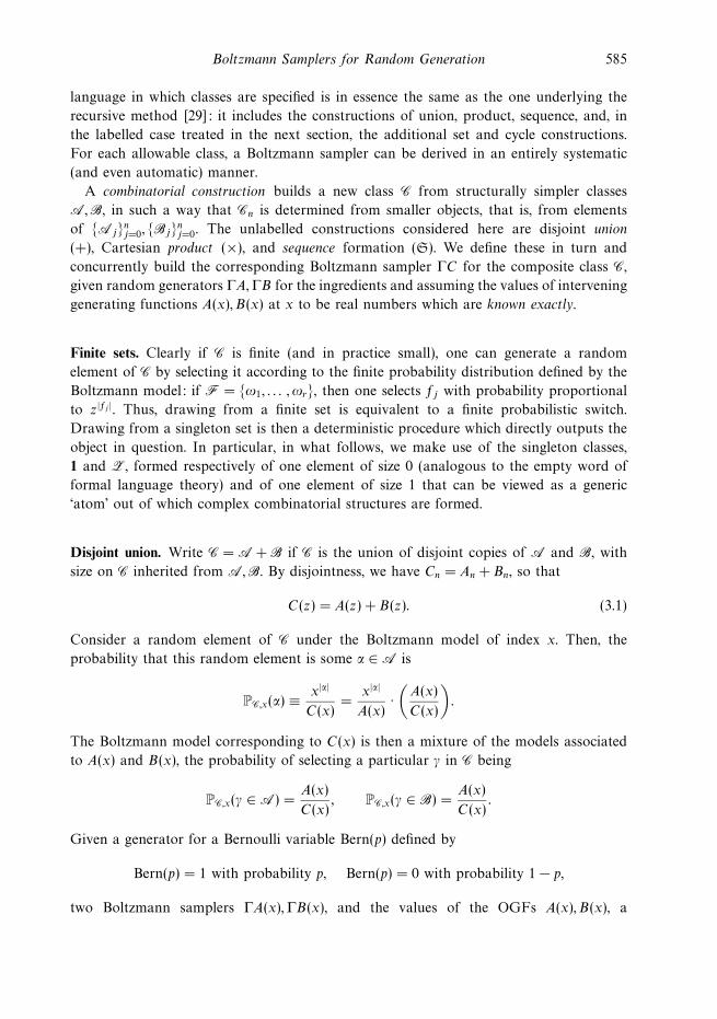
Disjoint union. Write C = A + B if C is the union of disjoint copies of A and B, with
size on C inherited from A,B. By disjointness, we have Cn = An + Bn, so that
C(z) = A(z) + B(z). (3.1)
Consider a random element of C under the Boltzmann model of index x. Then, the
probability that this random element is some α ∈ A is
PC,x(α) ≡ x|α|
C(x)=
x|α|
A(x)·(A(x)
C(x)
).
The Boltzmann model corresponding to C(x) is then a mixture of the models associated
to A(x) and B(x), the probability of selecting a particular γ in C being
PC,x(γ ∈ A) =A(x)
C(x), PC,x(γ ∈ B) =
A(x)
C(x).
Given a generator for a Bernoulli variable Bern(p) defined by
Bern(p) = 1 with probability p, Bern(p) = 0 with probability 1 − p,
two Boltzmann samplers ΓA(x),ΓB(x), and the values of the OGFs A(x), B(x), a
586 P. Duchon, P. Flajolet, G. Louchard and G. Schaeffer
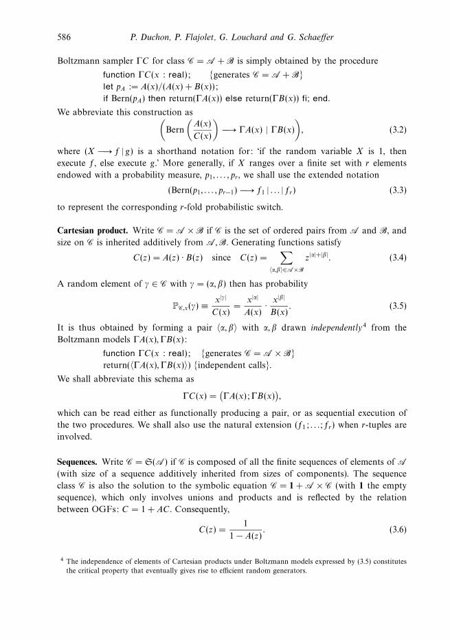
Boltzmann sampler ΓC for class C = A + B is simply obtained by the procedure
function ΓC(x : real); generates C = A + Blet pA := A(x)/(A(x) + B(x));
if Bern(pA) then return(ΓA(x)) else return(ΓB(x)) fi; end.
We abbreviate this construction as(Bern
(A(x)
C(x)
)−→ ΓA(x) | ΓB(x)
), (3.2)
where (X −→ f | g) is a shorthand notation for: ‘if the random variable X is 1, then
execute f, else execute g.’ More generally, if X ranges over a finite set with r elements
endowed with a probability measure, p1, . . . , pr , we shall use the extended notation
(Bern(p1, . . . , pr−1) −→ f1 | . . . | fr) (3.3)
to represent the corresponding r-fold probabilistic switch.
Cartesian product. Write C = A × B if C is the set of ordered pairs from A and B, and
size on C is inherited additively from A,B. Generating functions satisfy
C(z) = A(z) · B(z) since C(z) =∑
〈α,β〉∈A×B
z|α|+|β|. (3.4)
A random element of γ ∈ C with γ = (α, β) then has probability
PC,x(γ) ≡ x|γ|
C(x)=
x|α|
A(x)· x
|β|
B(x). (3.5)
It is thus obtained by forming a pair 〈α, β〉 with α, β drawn independently4 from the
Boltzmann models ΓA(x),ΓB(x):
function ΓC(x : real); generates C = A × Breturn(〈ΓA(x),ΓB(x)〉) independent calls.
We shall abbreviate this schema as
ΓC(x) =(ΓA(x); ΓB(x)
),
which can be read either as functionally producing a pair, or as sequential execution of
the two procedures. We shall also use the natural extension (f1; . . .; fr) when r-tuples are
involved.
Sequences. Write C = S(A) if C is composed of all the finite sequences of elements of A(with size of a sequence additively inherited from sizes of components). The sequence
class C is also the solution to the symbolic equation C = 1 + A × C (with 1 the empty
sequence), which only involves unions and products and is reflected by the relation
between OGFs: C = 1 + AC . Consequently,
C(z) =1
1 − A(z). (3.6)
4 The independence of elements of Cartesian products under Boltzmann models expressed by (3.5) constitutes
the critical property that eventually gives rise to efficient random generators.
Boltzmann Samplers for Random Generation 587
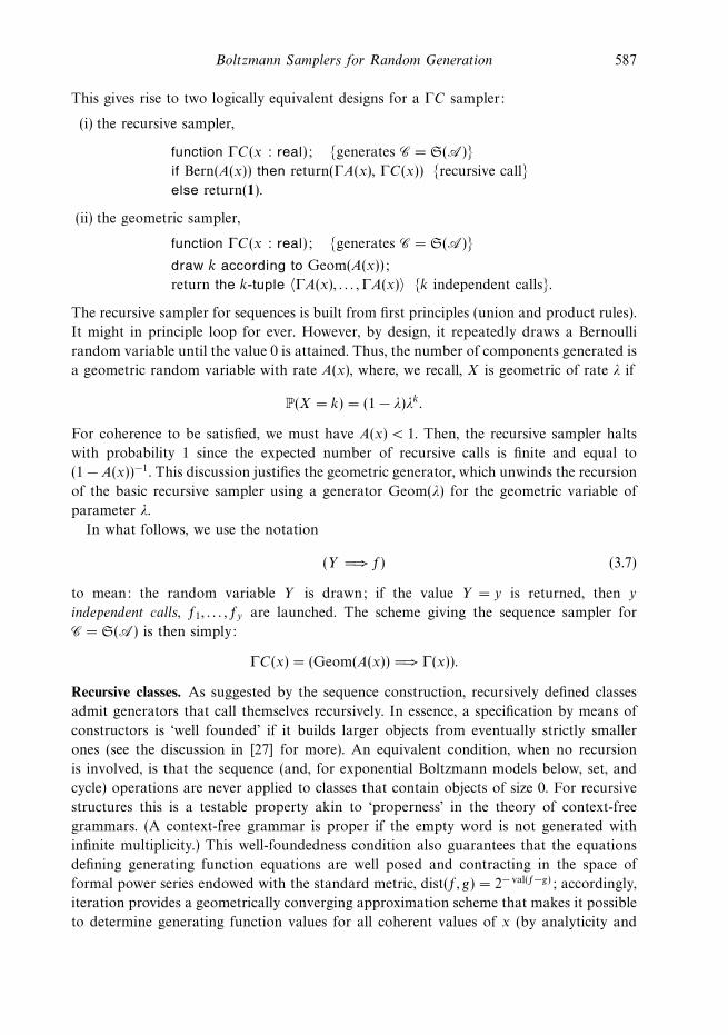
This gives rise to two logically equivalent designs for a ΓC sampler:
(i) the recursive sampler,
function ΓC(x : real); generates C = S(A)if Bern(A(x)) then return(ΓA(x), ΓC(x)) recursive callelse return(1).
(ii) the geometric sampler,
function ΓC(x : real); generates C = S(A)draw k according to Geom(A(x));
return the k-tuple 〈ΓA(x), . . . ,ΓA(x)〉 k independent calls.
The recursive sampler for sequences is built from first principles (union and product rules).
It might in principle loop for ever. However, by design, it repeatedly draws a Bernoulli
random variable until the value 0 is attained. Thus, the number of components generated is
a geometric random variable with rate A(x), where, we recall, X is geometric of rate λ if
P(X = k) = (1 − λ)λk.
For coherence to be satisfied, we must have A(x) < 1. Then, the recursive sampler halts
with probability 1 since the expected number of recursive calls is finite and equal to
(1 − A(x))−1. This discussion justifies the geometric generator, which unwinds the recursion
of the basic recursive sampler using a generator Geom(λ) for the geometric variable of
parameter λ.
In what follows, we use the notation
(Y =⇒ f) (3.7)
to mean: the random variable Y is drawn; if the value Y = y is returned, then y
independent calls, f1, . . . , fy are launched. The scheme giving the sequence sampler for
C = S(A) is then simply:
ΓC(x) = (Geom(A(x)) =⇒ Γ(x)).
Recursive classes. As suggested by the sequence construction, recursively defined classes
admit generators that call themselves recursively. In essence, a specification by means of
constructors is ‘well founded’ if it builds larger objects from eventually strictly smaller
ones (see the discussion in [27] for more). An equivalent condition, when no recursion
is involved, is that the sequence (and, for exponential Boltzmann models below, set, and
cycle) operations are never applied to classes that contain objects of size 0. For recursive
structures this is a testable property akin to ‘properness’ in the theory of context-free
grammars. (A context-free grammar is proper if the empty word is not generated with
infinite multiplicity.) This well-foundedness condition also guarantees that the equations
defining generating function equations are well posed and contracting in the space of
formal power series endowed with the standard metric, dist(f, g) = 2− val(f−g); accordingly,
iteration provides a geometrically converging approximation scheme that makes it possible
to determine generating function values for all coherent values of x (by analyticity and
588 P. Duchon, P. Flajolet, G. Louchard and G. Schaeffer
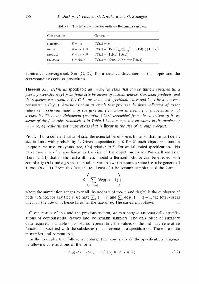
Table 3. The inductive rules for ordinary Boltzmann samplers.
Construction Generator
singleton C = ω ΓC(x) = ω
union C = A + B ΓC(x) =(Bern
( A(x)A(x)+B(x)
)−→ ΓA(x) | ΓB(x)
)product C = A × B ΓC(x) =
(ΓA(x); ΓB(x)
)sequence C = S(A) ΓC(x) =
(Geom(A(x)) =⇒ ΓA(x)
)
dominated convergence). See [27, 29] for a detailed discussion of this topic and the
corresponding decision procedures.
Theorem 3.1. Define as specifiable an unlabelled class that can be finitely specified (in a
possibly recursive way) from finite sets by means of disjoint unions, Cartesian products, and
the sequence construction. Let C be an unlabelled specifiable class and let x be a coherent
parameter in (0, ρC ). Assume as given an oracle that provides the finite collection of exact
values at a coherent value x of the generating functions intervening in a specification of
a class C. Then, the Boltzmann generator ΓC(x) assembled from the definition of C by
means of the four rules summarized in Table 3 has a complexity measured in the number of
(+,−,×,÷) real-arithmetic operations that is linear in the size of its output object.
Proof. For a coherent value of size, the expectation of size is finite, so that, in particular,
size is finite with probability 1. Given a specification Σ for C, each object ω admits a
unique parse tree (or syntax tree) τ[ω] relative to Σ. For well-founded specifications, this
parse tree τ is of a size linear in the size of the object produced. We shall see later
(Lemma 5.1) that in the real-arithmetic model a Bernoulli choice can be effected with
complexity O(1) and a geometric random variable which assumes value k can be generated
at cost O(k + 1). From this fact, the total cost of a Boltzmann sampler is of the form
O
∑ν∈τ[ω]
(deg(ν) + 1)
,where the summation ranges over all the nodes ν of tree τ, and deg(ν) is the outdegree of
node ν. Since, for any tree τ, we have∑
ν 1 = |τ| and∑
ν deg(ν) = |τ| − 1, the total cost is
linear in the size of τ, hence linear in the size of ω. The statement follows.
Given results of this and the previous section, we can compile automatically specific-
ations of combinatorial classes into Boltzmann samplers. The only piece of auxiliary
data required is a table of constants representing the values of the ordinary generating
functions associated with the subclasses that intervene in a specification. These are finite
in number and computable.
In the examples that follow, we enlarge the expressivity of the specification language
by allowing constructions of the form
SΩ(A) = 〈α1, . . . , αr〉 | αj ∈ A, r ∈ Ω, (3.8)
Boltzmann Samplers for Random Generation 589
where Ω ⊂ N is either a finite or a cofinite subset of the integers. If Ω is finite, this
construction reduces to a disjunction of finitely many cases and the corresponding sampler
is obtained by Bernoulli trials. If Ω is cofinite, we may assume without loss of generality
that Ω = n m0 for some m0 ∈ N, in which case the construction Sm0(A) reduces to
Am0 × S(A).
Example 1 (Words without long runs). Consider the collection R of all binary words
over the alphabet A = a, b that never have more than m consecutive occurrences of
any letter (such consecutive sequences are also called ‘runs’ and intervene at many places
in statistics, coding theory, and genetics). Here we regard m as a fixed quantity. It is not
a priori obvious how to generate a random word in R of length n: a brutal rejection
method based on generating random unconstrained words and filtering out those that
satisfy the condition R will not work in polynomial time since the constrained words
have an exponentially small probability. On the other hand, any word decomposes into a
sequence of alternations also called its core, of the form
(aa · · · a | bb · · · b) (aa · · · a | bb · · · b) · · · (aa · · · a | bb · · · b), (3.9)
possibly prefixed with a header of b s and postfixed with a trailer of a s. In symbols, the
set W of all words is expressible by a regular expression, written in our notation
W = S(b) × S(aS(a)bS(b)) × S(a).
The decomposition was customized to serve for R: simply replace any internal aS(a) by
S1 . . m(a) and any bS(b) by S1 . . m(b), where S1 . . m means a sequence of between 1 and m
elements, and adapt accordingly the header and trailer:
R = Sm(b) × S(S1 . . m(a)S1 . . m(b)) × Sm(a).
The composition rules given above give rise to a generator for R that has the following
form: two generators that produce sequences of a s or b s according to a truncated
geometric law; a generator for the product C := (S1 . . m(a)S1 . . m(b)) that is built according
to the product rule; a generator for the sequence D := S(C) constructed according to the
sequence rule. The generator finally assembled automatically is
ΓR(x) = (X =⇒ b); ΓCore(x); (X ′ =⇒ a),
ΓCore(x) =(
Geom(x2(1 − xm)2
(1 − x)2
)=⇒
((Y =⇒ a); (Y ′ =⇒ b)
))X,X ′ ∈ Geom
m(x), Y , Y ′ ∈ Geom
1 . . m(x).
Observe that a table of only a small number of real-valued constants rationally related
to x and including
c1 = x, c2 = C(x) = x2(1 − xm)2(1 − x)−2,
needs to be precomputed in order to implement the algorithm.
590 P. Duchon, P. Flajolet, G. Louchard and G. Schaeffer
Here are three runs of the sampler ΓR(x) for m = 4 produced with the coherent value
x = 0.5 (the critical value is ρR.
= 0.51879), of respective lengths 124 (truncated), 23, and
35, with the coding a =, b = :
· · ·
With this value of the parameter, the mean size of a random word produced is about
27. The distribution turns out to be of the ‘flat’ type, as for surjections in Figure 1. We
shall see later in Section 7 that one can design optimized samplers for such types of
distributions. The technique applies to any language composed of words with excluded
patterns, meaning words that are constrained not to contain any of a finite set of words
as factor. (For such a language, one can specifically construct a finite automaton by way
of the Aho–Corasick construction [1], then write the automaton as a linear system of
equations relating specifications, and finally compile the set of equations into a recursive
Boltzmann sampler.) More generally, the method applies to any regular language: it
suffices to convert a description of the language into a deterministic finite automaton and
apply the recursive construction of a sampler, or alternatively to obtain an unambiguous
regular expression and derive from it a nonrecursive sampler based on the geometric law.
The next set of examples is relative to structures that satisfy nonlinear recursive
descriptions of the context-free type.
Example 2 (Rooted plane trees). Take the class B of binary trees defined by the recursive
specification
B = Z + (Z × B × B),
where Z is the class comprising the generic node. The generator ΓZ is deterministic and
consists simply of the instruction ‘output a node’ (since Z is finite and in fact has only
one element). The Boltzmann generator ΓB calls ΓZ (and halts) with probability x/B(x)
where B(x) is the OGF of binary trees,
B(x) =1 −
√1 − 4x2
2x.
With the complementary probability corresponding to the strict binary case, it will make a
call to ΓZ and two recursive calls to itself. In shorthand notation, the recursive sampler is
ΓB(x) =(
Bern(
xB(x)
)−→ Z |
(Z; ΓB(x); ΓB(x)
)).
In other words: the Boltzmann generator for binary trees as constructed automatically from
the composition rules produces a random sample of the branching process with probabilities
( xB(x)
, xB(x)2
B(x)). Note that the generator is defined for x < 1/2 (the radius of convergence
of B(x)), in which case the branching process is subcritical, so that the algorithm halts
in finite expected time, as it should. Only two constants are needed for implementation,
namely x and the quadratic irrational xB(x)
.
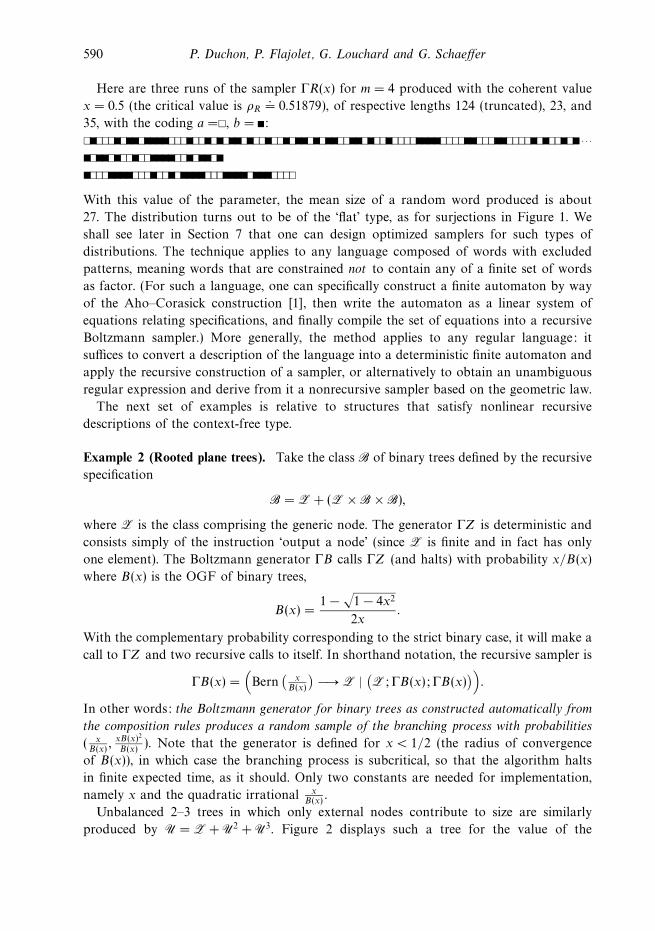
Unbalanced 2–3 trees in which only external nodes contribute to size are similarly
produced by U = Z + U2 + U3. Figure 2 displays such a tree for the value of the
Boltzmann Samplers for Random Generation 591
Figure 2. Random unbalanced 2–3 trees of 173 and 2522 nodes (in total) produced by a critical
Boltzmann sampler
parameter x set at the critical value ρU = 527
. (This critical value can be determined by
methods exposed in Section 7.) In this case, the branching probabilities for a nullary,
binary, and ternary node are found to be, respectively,
p0 =5
9, p2 =
1
3, p3 =
1
9,
and these three constants are the only ones required by the algorithm. A typical run of
30 Boltzmann samplings produces trees with total number of nodes equal to
3, 6, 1, 1, 6, 7, 33, 1, 1, 1, 9, 1, 1, 3, 1, 3, 169, 1881, 1, 54, 6, 1, 1, 3, 3746, 1, 1, 1, 1, 1, (3.10)
which empirically gives an indication of the distribution of sizes (it turns out to be of
the peaked type, like in Figure 1, bottom). We shall see later in Section 7 that one can
actually characterize the profile of this distribution (it decays like n−3/2) and put to good
use some of its features.
Unary-binary trees (also known as Motzkin trees) are defined by V = Z(1 + V + V2).
General plane trees, G, where all degrees of nodes are allowed, can be specified by the
grammar
G = Z × S(G),
with OGF G(z) = (1 −√
1 − 4z)/2. Accordingly, the automatically produced sampler is
ΓG(x) = (Z; (Geom(G(x)) =⇒ ΓG(x))),
which corresponds to the well-known fact that such trees are equivalent to trees of a
branching process where the offspring distribution is geometric.
592 P. Duchon, P. Flajolet, G. Louchard and G. Schaeffer
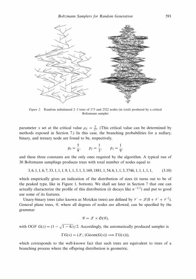
Figure 3. A random connected non-crossing graph of size 50
Example 3 (Secondary structures). This example is inspired by works of Waterman et al.,
themselves motivated by the problem of enumerating secondary RNA structures [36, 62].
To fix ideas, consider rooted binary trees where edges contain 2 or 3 atoms and leaves
(‘loops’) contain 4 or 5 atoms. A specification is W = (Z4 + Z5) + (Z2 + Z3)2 × (W ×W). A Bernoulli switch will decide whether to halt or not, two independent recursive
calls being made in case it is decided to continue, with the algorithm being sugared with
suitable Bernoulli draws. Here is the complete code:
ΓA(x) =(Bern
(x4
x4 + x5
)−→ Z4 | Z5
),
ΓB(x) =(Bern
(x2
x2 + x3
)−→ Z2 | Z3
),
let p = (x4 + x5)/W (x) = 12(1 +
√1 − 4x8(1 + x)3),
ΓW (x) =(Bern(p) −→ ΓA(x) | ΓB(x); ΓW (x); ΓB(x); ΓW (x)
).
The method is clearly universal for this entire class of problems.
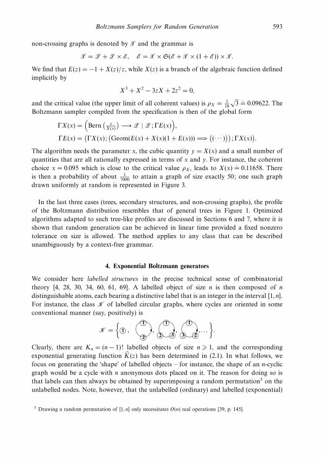
Example 4 (Non-crossing graphs). Consider graphs which, for size n, have vertices at
the nth roots of unity, vk = e2ikπ/n, and are connected and non-crossing in the sense that
no two edges are allowed to meet in the interior of the unit circle; see Figure 3 for a
random instance. The generating function of such graphs was first determined by Domb
and Barrett [15], motivated by the investigation of certain perturbative expansions of
statistical physics. Their derivation is not based on methods conducive to Boltzmann
sampling, though. On the other hand, the planar structure of such configurations entails
a neat decomposition, which is described in [24]. At the top level, consider the graph
as rooted at vertex v0. Let vi and vj be two consecutive neighbours of v0; the subgraph
induced on the vertex set vi, vi+1, . . . , vj is either a connected graph of D or is formed of
two disjoint components containing vi and vj respectively. Also, if v is the first neighbour
of v0 and vm is the last neighbour, there are two connected components on v1, . . . , v and on vm, . . . , vn−1 respectively. The grammar for connected non-crossing graphs is then
a transcription of this simple decomposition, although its detail is complicated as care
must be exercised to avoid double counting of vertices. The class of all such connected
Boltzmann Samplers for Random Generation 593
non-crossing graphs is denoted by X and the grammar is
X = Z + Z × E, E = X × S(E + X × (1 + E)) × X.
We find that E(z) = −1 +X(z)/z, while X(z) is a branch of the algebraic function defined
implicitly by
X3 +X2 − 3zX + 2z2 = 0,
and the critical value (the upper limit of all coherent values) is ρX = 118
√3.
= 0.09622. The
Boltzmann sampler compiled from the specification is then of the global form
ΓX(x) =(
Bern(
xX(x)
)−→ Z | Z; ΓE(x)
),
ΓE(x) =(ΓX(x);
(Geom(E(x) +X(x)(1 + E(x))) =⇒
((· · · )
)); ΓX(x)
).
The algorithm needs the parameter x, the cubic quantity y = X(x) and a small number of
quantities that are all rationally expressed in terms of x and y. For instance, the coherent
choice x = 0.095 which is close to the critical value ρX , leads to X(x).
= 0.11658. There
is then a probability of about 17000
to attain a graph of size exactly 50; one such graph
drawn uniformly at random is represented in Figure 3.
In the last three cases (trees, secondary structures, and non-crossing graphs), the profile
of the Boltzmann distribution resembles that of general trees in Figure 1. Optimized
algorithms adapted to such tree-like profiles are discussed in Sections 6 and 7, where it is
shown that random generation can be achieved in linear time provided a fixed nonzero
tolerance on size is allowed. The method applies to any class that can be described
unambiguously by a context-free grammar.
4. Exponential Boltzmann generators
We consider here labelled structures in the precise technical sense of combinatorial
theory [4, 28, 30, 34, 60, 61, 69]. A labelled object of size n is then composed of n
distinguishable atoms, each bearing a distinctive label that is an integer in the interval [1, n].
For instance, the class K of labelled circular graphs, where cycles are oriented in some
conventional manner (say, positively) is
K =
1 ,
12 ,
12 3 ,
13 2 , . . .
.
Clearly, there are Kn = (n− 1)! labelled objects of size n 1, and the corresponding
exponential generating function K(z) has been determined in (2.1). In what follows, we
focus on generating the ‘shape’ of labelled objects – for instance, the shape of an n-cyclic
graph would be a cycle with n anonymous dots placed on it. The reason for doing so is
that labels can then always be obtained by superimposing a random permutation5 on the
unlabelled nodes. Note, however, that the unlabelled (ordinary) and labelled (exponential)
5 Drawing a random permutation of [1, n] only necessitates O(n) real operations [39, p. 145].
594 P. Duchon, P. Flajolet, G. Louchard and G. Schaeffer
Boltzmann models assign rather different probabilities to objects: in the unlabelled case,
there would be only kn ≡ 1 object of size n, with OGF k(x) = x/(1 − x) so that the
distribution of component sizes is geometric, while in the labelled case, the logarithmic
series distribution (2.2) occurs.
Labelled combinatorial classes can be subjected to the labelled product defined as
follows: if A and B are labelled classes, the product C = A B is obtained by forming
all ordered pairs 〈α, β〉 with α ∈ A and β ∈ B and relabelling them in all possible
order-consistent ways. Straight from the definition, we have a binomial convolution Cn =∑nk=0
(nk
)AkBn−k, where the binomial takes care of relabellings. In terms of exponential
generating functions, this becomes
C(z) = A(z) · B(z).
As in the ordinary case, we proceed by assembling Boltzmann generators for structured
objects from simpler ones.
Disjoint union. The unlabelled construction carries over verbatim to this case to the
effect that, for labelled classes A,B,C satisfying C = A + B, EGFs are related by
C(z) = A(z) + B(z), and the exponential Boltzmann sampler for C is
ΓC(x) =(
Bern(
A(x)
A(x) + B(x)
)−→ ΓA(x) | ΓB(x)
).
Labelled product. The Cartesian product construction adapts to this case with minor
modifications: to produce an element from C = A B, simply produce a pair by the
Cartesian product rule using values A(x), B(x):
ΓC(x) = (ΓA(x); ΓB(x)).
Complete by a randomly chosen relabelling if actual values of the labels are needed.
Sequences. In the labelled universe, C is the sequence class of A, written C = S(A) if
and only if it is composed of all the sequences of elements from A up to order-consistent
relabellings. Then, the EGF relation
C(x) =∑k0
A(x)k =1
1 − A(x)
holds, and either of the two constructions of the generator ΓC from ΓA given in Section 3
is applicable. In particular, the nonrecursive generator is
ΓC(x) = (Geom(A(x)) =⇒ ΓA(x)),
where the stenographic convention of (3.7) is employed.
Sets. This is a new construction that we did not consider in the unlabelled case. The class
C is the set-class of A, written C = P(A) (P is reminiscent of ‘powerset’) if C is the
quotient of sequences, C = S(A)/ ≡, by the relation ≡ that declares two sequences as
equivalent if one derives from the other by an arbitrary permutation of the components.
Boltzmann Samplers for Random Generation 595
It is then easily seen that the EGFs are related by
C(x) =∑k0
1
k!A(x)k = eA(x),
where the factor 1/k! ‘kills’ the order present in k-sequences.
The Poisson law of rate λ is classically defined by
P(X = k) = e−λ λk
k!.
On the other hand, under the exponential Boltzmann, the probability for a set in C to
have k components in A is
1
C(x)
1
k!A(x)k = e−A(x) A(x)k
k!,
that is, a Poisson law of rate A(x). This gives rise to a simple algorithm for generating
sets (analogous to the geometric algorithm for sequences):
ΓC(x) =(Pois(A(x)) =⇒ ΓA(x)
).
Cycles. This construction, written C = C(A), is defined like sets but with two sequences
being identified if one is a cyclic shift of the other. The EGFs satisfy
C(x) =∑k1
1
kA(x)k = log
1
1 − A(x),
where the factor 1/k ‘converts’ k-sequences into k-cycles. The log-law of rate λ < 1, an
‘integral’ of the geometric law also known as the logarithmic series distribution, is the law
of a variable X such that
P(X = k) =1
log(1 − λ)−1
λk
k.
(This is the same as in equation (2.2); the distribution occurs in statistical ecology and
economy and forms the subject of Chapter 7 of [38].) Then cycles under the exponential
Boltzmann model can be drawn like in the case of sets upon replacing the Poisson law
by the log-law:
ΓC(x) =(Loga(A(x)) =⇒ ΓA(x)
).
These constructions are summarized in Table 4.
For reasons identical to those that justify Theorem 3.1, we have the following.
Theorem 4.1. Define as specifiable a labelled class that can be finitely specified (in a
possibly recursive way) from finite sets by means of disjoint unions, Cartesian products,
as well as the sequence, set and cycle constructions. Let C be a labelled specifiable class
and x be a coherent parameter in (0, ρC ). Assume as given an oracle that provides the finite
collection of exact values at a coherent value x of the generating functions intervening
in a specification of a class C. Then, the Boltzmann generator ΓC(x) assembled from the
596 P. Duchon, P. Flajolet, G. Louchard and G. Schaeffer
Table 4. The inductive rules for exponential Boltzmann samplers
Construction Generator
singleton C = ω ΓC(x) = ω
union C = A + B ΓC(x) =(Bern
( A(x)
A(x)+B(x)
)−→ ΓA(x) | ΓB(x)
)product C = A B ΓC(x) =
(ΓA(x); ΓB(x)
)sequence C = S(A) ΓC(x) =
(Geom(A(x)) =⇒ ΓA(x)
)set C = P(A) ΓC(x) =
(Pois(A(x)) =⇒ ΓA(x)
)cycle C = C(A) ΓC(x) =
(Loga(A(x)) =⇒ ΓA(x)
)
definition of C by means of the six rules of Table 4 has a complexity measured in the number
of (+,−,×,÷) real-arithmetic operations that is linear in the size of its output object.
(We also allow constructions SΩ,PΩ,CΩ as in (3.8); in this case, the random variable
of geometric, Poisson, or logarithmic type should be conditioned to assume its values in
the set Ω.)
As in the unlabelled case, Boltzmann samplers can be compiled automatically from
combinatorial specifications. There is here added expressivity in the specification language,
thanks to the inclusion of the Set and Cycle constructions. In the examples that follow,
we omit the hat-marker ‘f’, whenever the exponential/labelled character of the model is
clear from the context.
Example 5 (Set partitions). A set partition of size n is a partition of the integer interval
[1, n] into a certain number of nonempty classes, also called blocks, the blocks being by
definition unordered between themselves. Let P1 represent the powerset construction
where the number of components is constrained to be 1. (This modified construction is
easily subjected to random generation by using a truncated Poisson variable K , where K
is conditioned to be 1.) The labelled class of all set partitions is then definable as
S = P(P1(Z)), where Z consists of a single labelled atom, Z = 1. Observe that the
EGF of S is the well-known generating function of the Bell numbers, S(z) = eez−1. By
the composition rules, we get a random generator as follows. Choose the number K of
blocks as Poisson(ex − 1). Draw K independent copies X1, X2, . . . , XK from the Poisson law
of rate x, but each conditioned to be at least 1. In symbols:
ΓS(x) =(
Pois(ex − 1) =⇒(
Pois1
(x) =⇒ Z)).
What this generates is in reality the ‘shape’ of a set partition (the number of blocks (K)
and the block sizes (Xj)), with the ‘correct’ distribution. To complete the task, it suffices
to transport this structure on a random permutation of the integers between 1 and N,
where N = X1 + · · · +XK .
The process markedly differs from the classical algorithm of Nijenhuis and Wilf [51]
that requires tables of large integers. It is related to a continuous model devised by

Boltzmann Samplers for Random Generation 597
Figure 4. A random partition obtained by the Boltzmann parameter of parameter x = 6, here of size n =
2356 and comprising 409 blocks: (left) the successive block sizes generated, (right) the block sizes in sorted
order
Vershik [67] that can be interpreted as generating random set partitions based on
S(x) = ex/1! · ex2/2! · ex3/3! · · · ,
i.e., by ordered block lengths, as a potentially infinite sequence of Poisson variables of
parameters x/1!, x2/2!, and so on.
Figure 4 represents a random set partition produced by the Boltzmann model of
parameter x = 6. This particular object has size n = 2356, the expected size being Ex(N) =
2420 for this value of the parameter. The closeness between the observed size and its
mean value agrees with the concentration that is perceptible on Figure 1. In addition, the
Boltzmann model immediately provides a simple heuristic model of partitions of large
size. Objects of size ‘near’ n, are produced by the value xn defined by xnexn = n, that is,
xn ≈ log n− log log n. Then, the number of blocks is expected to be about exn ≈ n/(log n).
This number being large, and individual blocks being generated by independent Poisson
variables of parameter xn, we expect, for large n, the sorted profile of blocks (Figure 4,
right) to converge to the histogram of the Poisson distribution of rate xn. As shown by
Vershik [67], this heuristic model is indeed a valid asymptotic model of partitions of large
sizes.
Example 6 (Random surjections, or ordered set partitions). These may be defined as
functions from [1, n] to [1, n] such that the image of f is an initial segment of [1, n]
(i.e., there are no ‘gaps’). For the class Q of surjections we have Q = S(P1(Z)). Thus a
random generator for Q is
ΓQ(x) =(
Geom(ex − 1) =⇒(
Pois1
(x) =⇒ Z)).
In words: first choose a number of components given by a geometric law and then launch
a number of Poisson generators conditioned to be at least 1.
598 P. Duchon, P. Flajolet, G. Louchard and G. Schaeffer
Set partitions find themselves attached to a compound (PoissonPoisson) process,
whereas surjections are generated by a compound (GeometricPoisson) process (with
suitable dependencies on parameters). This reflects the basic combinatorial opposition
between freedom and order (for blocks). Here are two more examples.
Example 7 (Cycles in permutations). This corresponds to P = P(C1(Z)) and is obtained
by a (PoissonLog) process:
ΓP (x) =(Pois(log(1 − x)−1) =⇒ (Loga(x) =⇒ Z)
).
This example is related to the Shepp–Lloyd model [57] that generates permutations by
ordered cycle lengths, as a potentially infinite sequence of Poisson variables of parameters
x/1, x2/2, and so on. The interest of this construction is to give rise to a number of
useful particularizations. For instance derangements (permutations such that σ(x) = x)
are produced by P = P(C2(Z)); involutions (permutations such that σ σ(x) = x) are
given by P = P(C1 . . 2(Z)).
Example 8 (Assemblies of filaments). Imagine assemblies of linear filaments floating
freely in a liquid. We may model these as sets of sequences, F = P(S1(Z)). The EGF
is exp( z1 − z
). The random generation algorithm is a compound of the form (PoissonGeometric), with appropriate parameters:
ΓF(x) =(
Pois(
x1 − x
)=⇒
(Geom
1(x) =⇒ Z
)).
The corresponding counting sequence, 1, 1, 3, 13, 73, 501, . . . , appears as A000262 in
Sloane’s encyclopedia [58]. This example is closely related to linear forests and posets as
described in Burris’s book (see [6], pp. 23–24 and Chapter 4).
At this stage, it may be of interest to note that many classical distributions of probability
theory can be retrieved as (size distributions of) Boltzmann models associated to simple
combinatorial games. Consider an unbounded supply of distinguishable (i.e., labelled)
balls. View an urn as an unordered finite collection of balls (P(Z)) and a stack as
an ordered collection of balls (S(Z)). The geometric and Poisson distributions arise as
the size distributions of the stack and the urn. If, by an exclusion principle, an urn
is only allowed to contain 0 or 1 ball (1 + Z), then the family of all basic Bernoulli
distributions results. If m urns or stacks are considered, then the distributions are Poisson
or negative binomial, respectively, and, with exclusion, we get in this way the binomial
distributions corresponding to m trials. If balls and urns are taken to be indistinguishable,
we automatically obtain Vershik’s model of integer partitions [67], which is an infinite
product of geometric distributions of exponentially decaying rates. (The recent work by
Milenkovic and Compton [50] discusses exact and asymptotic transforms associated to
several such distributions.) For similar reasons, the two classical models of random graphs
due to Erdos and Renyi are related to one another by ‘Boltzmannization’. A large number
of examples along similar lines could clearly be listed.
Boltzmann Samplers for Random Generation 599
5. The realization of Boltzmann samplers
In this section, we make explicit the way Boltzmann sampling can be implemented and
sketch a discussion of the main complexity issues involved. Broadly speaking, samplers
can be realized under two types of computational models corresponding to computations
carried out over the set R of real numbers or the set S = 0, 1N of infinite-length binary
strings. (In the latter case, only finite prefixes are ever used.) These are the real-arithmetic
model, R, which is the one considered here and the bit string model (or Boolean model),
S, whose algorithms will be described in a future publication. The ‘ideal’ real-domain
model R comprises the elementary operations +,−,×,÷ each taken to have unit cost.
By definition, a Boltzmann sampler requires as input the value of the control parameter x
that defines the Boltzmann model of use. As seen in previous sections, it also needs the
finite collection of values at x of the generating functions that intervene in a specification,
in order to drive Bernoulli, geometric, Poisson, and logarithmic generators. We assume
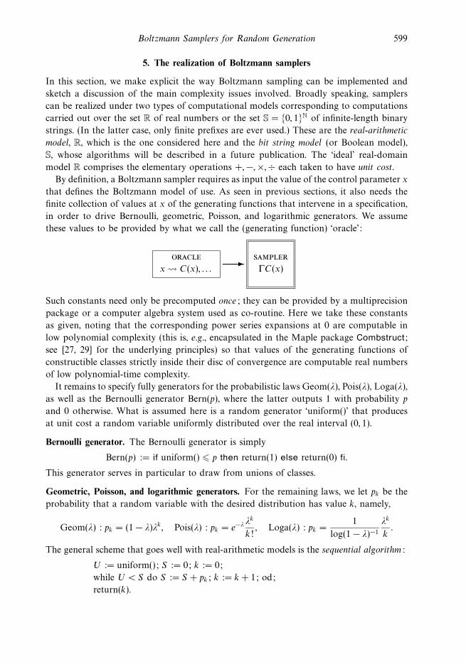
these values to be provided by what we call the (generating function) ‘oracle’:
oracle
x C(x), . . .
sampler
ΓC(x)
Such constants need only be precomputed once; they can be provided by a multiprecision
package or a computer algebra system used as co-routine. Here we take these constants
as given, noting that the corresponding power series expansions at 0 are computable in
low polynomial complexity (this is, e.g., encapsulated in the Maple package Combstruct;
see [27, 29] for the underlying principles) so that values of the generating functions of
constructible classes strictly inside their disc of convergence are computable real numbers
of low polynomial-time complexity.
It remains to specify fully generators for the probabilistic laws Geom(λ), Pois(λ), Loga(λ),
as well as the Bernoulli generator Bern(p), where the latter outputs 1 with probability p
and 0 otherwise. What is assumed here is a random generator ‘uniform()’ that produces
at unit cost a random variable uniformly distributed over the real interval (0, 1).
Bernoulli generator. The Bernoulli generator is simply
Bern(p) := if uniform() p then return(1) else return(0) fi.
This generator serves in particular to draw from unions of classes.
Geometric, Poisson, and logarithmic generators. For the remaining laws, we let pk be the
probability that a random variable with the desired distribution has value k, namely,
Geom(λ) : pk = (1 − λ)λk, Pois(λ) : pk = e−λ λk
k!, Loga(λ) : pk =
1
log(1 − λ)−1
λk
k.
The general scheme that goes well with real-arithmetic models is the sequential algorithm:
U := uniform(); S := 0; k := 0;
while U < S do S := S + pk; k := k + 1; od;
return(k).
600 P. Duchon, P. Flajolet, G. Louchard and G. Schaeffer
Table 5.
Geom(λ) Pois(λ) Loga(λ)
p0 = (1 − λ) p0 = e−λ p1 = 1/(log(1 − λ)−1)
pk+1 = λpk pk+1 = λpk1
k+ 1 pk+1 = λpkk
k+ 1 .
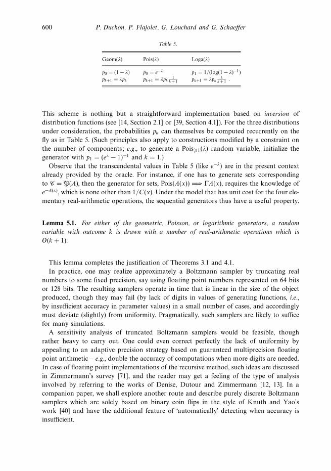
This scheme is nothing but a straightforward implementation based on inversion of
distribution functions (see [14, Section 2.1] or [39, Section 4.1]). For the three distributions
under consideration, the probabilities pk can themselves be computed recurrently on the
fly as in Table 5. (Such principles also apply to constructions modified by a constraint on
the number of components; e.g., to generate a Pois1(λ) random variable, initialize the
generator with p1 = (eλ − 1)−1 and k = 1.)
Observe that the transcendental values in Table 5 (like e−λ) are in the present context
already provided by the oracle. For instance, if one has to generate sets corresponding
to C = P(A), then the generator for sets, Pois(A(x)) =⇒ ΓA(x), requires the knowledge of
e−A(x), which is none other than 1/C(x). Under the model that has unit cost for the four ele-
mentary real-arithmetic operations, the sequential generators thus have a useful property.
Lemma 5.1. For either of the geometric, Poisson, or logarithmic generators, a random
variable with outcome k is drawn with a number of real-arithmetic operations which is
O(k + 1).
This lemma completes the justification of Theorems 3.1 and 4.1.
In practice, one may realize approximately a Boltzmann sampler by truncating real
numbers to some fixed precision, say using floating point numbers represented on 64 bits
or 128 bits. The resulting samplers operate in time that is linear in the size of the object
produced, though they may fail (by lack of digits in values of generating functions, i.e.,
by insufficient accuracy in parameter values) in a small number of cases, and accordingly
must deviate (slightly) from uniformity. Pragmatically, such samplers are likely to suffice
for many simulations.
A sensitivity analysis of truncated Boltzmann samplers would be feasible, though
rather heavy to carry out. One could even correct perfectly the lack of uniformity by
appealing to an adaptive precision strategy based on guaranteed multiprecision floating
point arithmetic – e.g., double the accuracy of computations when more digits are needed.
In case of floating point implementations of the recursive method, such ideas are discussed
in Zimmermann’s survey [71], and the reader may get a feeling of the type of analysis
involved by referring to the works of Denise, Dutour and Zimmermann [12, 13]. In a
companion paper, we shall explore another route and describe purely discrete Boltzmann
samplers which are solely based on binary coin flips in the style of Knuth and Yao’s
work [40] and have the additional feature of ‘automatically’ detecting when accuracy is
insufficient.
Boltzmann Samplers for Random Generation 601
6. Exact-size and approximate-size sampling
Our primary objective in this article is the fast random generation of objects of some
large size. In this section and the next one, we consider two types of constraints on size.
• Exact-size random sampling, where objects of C should be drawn uniformly at random
from the subclass Cn of objects of size exactly n.
• Approximate-size random sampling, where objects should be drawn with size in an
interval of the form I(n, ε) = [n(1 − ε), n(1 + ε)], for some quantity ε 0 called the
(relative) tolerance. In applications, one is likely to consider cases where ε is a small
fixed number, like 0.05, corresponding to an uncertainty on sizes of ±5%. Though size
may fluctuate (within limits), sampling is still unbiased6 in the sense that two objects
with the same size are drawn with equal likelihood.
The conditions of exact and approximate-size sampling are automatically satisfied if one
filters the output of a Boltzmann generator by retaining only the elements that obey the
desired size constraint. (As a matter of fact, we have liberally made use of this feature
in previous examples, e.g., when selecting the trees of Figure 2 to be large enough.) Such
a filtering is simply achieved by a rejection technique. The main question then becomes:
‘When and how can the rejection strategy be reasonably efficient?’
The major conclusion of this section is that in many cases, including all the examples
seen so far, approximate-size sampling is achievable in linear time under the (exact)
real-arithmetic model. In addition, the constants appear to be not too large if a
‘reasonable’ tolerance on size is accepted. Precisely, we develop analyses and optimizations
corresponding to the three common types of distributions exemplified in Figure 1.
• For size distributions that are ‘bumpy’, the straight rejection strategy succeeds with
high probability in one trial, hence the linear-time complexity of approximate-size
Boltzmann sampling results (Section 6.1).
• For size distributions that are ‘flat’, the straight rejection strategy succeeds in O(1)
trials on average, a fact that again ensures linear-time complexity when a nonzero
tolerance on size is allowed (Section 6.2).
• For size distributions that are ‘peaked’ (at the origin), the technique of pointing may
be used to transform automatically specifications into equivalent ones of the flat type
(Section 6.3).
6.1. Size-control and rejection samplers
The basic rejection sampler denoted by µC(x; n, ε) uses a Boltzmann generator ΓC(x) for
the class C and is described as follows, for any x with 0 < x < ρC , n a target size and
ε 0 a relative tolerance:
function µC(x; n, ε);
Returns an object of C of size in I(n, ε) := [n(1 − ε), n(1 + ε)]
6 Objects drawn according to an approximate-size sampler are thus always uniform conditioned on their size.
We do not however impose conditions on the sizes of the objects drawn, so that the objects returned are not
in general uniform over the set of all objects having size in I(n, ε).
602 P. Duchon, P. Flajolet, G. Louchard and G. Schaeffer
repeat γ := ΓC(x) until |γ| ∈ I(n, ε);
return(γ); end.
The rejection sampler µC depends on a parameter x that one may choose arbitrarily
amongst all coherent values. It simply tries repeatedly until an object of satisfactory size
is produced. The case ε = 0 then gives exact-size sampling.
The outcome of a basic Boltzmann sampler has a random size N whose distribution is
described by Proposition 2.1. We have
Ex(N) = ν1(x), Ex(N2) = ν2(x), Ex(N
2) − Ex(N)2 = σ(x)2,
where σ represents standard deviation, with
ν1(x) := xC ′(x)
C(x), ν2(x) := x2C
′′(x)
C(x)+ x
C ′(x)
C(x), σ(x) =
√ν2(x) − ν1(x).
If x stays bounded away from the critical value ρC , then ν1(x) remains bounded, so
that the object drawn is likely to have a small size (on average and in probability). Thus,
values of x approaching the critical value ρ ≡ ρC have to be considered. Introduce the
Mean Value Condition as
Mean Value Condition: limx→ρ−
ν1(x) = +∞. (6.1)
(This condition is satisfied in particular when C(ρ−) = +∞.) Then a ‘natural tuning’ for
the rejection sampler consists in adopting as control parameter x the value xn that satisfies
xn is the root in (0, ρ) of n = xC ′(x)
C(x), (6.2)
which is uniquely determined. We then have the following.
Theorem 6.1. Let C be a combinatorial class and let ε be a fixed (relative) tolerance on
size. Assume the Mean Value Condition (6.1) and the following Variance Condition:
Variance Condition: limx→ρ−
σ(x)
ν1(x)= 0. (6.3)
Then, the rejection sampler µC(xn; n, ε) equipped with the value x = xn implicitly determined
by (6.2) succeeds in one trial with probability tending to 1 as n → ∞. In particular, if C is
specifiable, then the overall cost of approximate-size sampling is O(n) on average.
Proof. This is a direct consequence of Chebyshev’s inequalities.
The mean and variance conditions are satisfied by the class S of set partitions
(Example 5, observe concentration on Figure 1, top) and the class F of assemblies
of filaments (Example 8 and Figure 5). In effect, for set partitions, S, the exponential
generating function is entire, which corresponds to ρ = +∞. We find
ν1(x) = xex, σ(x)2 = x(x+ 1)ex, (6.4)
while xn determined implicitly by the equation xnexn = n satisfies
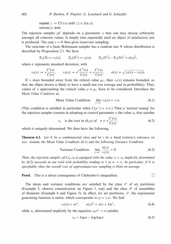
xn ∼ log n− log log n. (6.5)
Boltzmann Samplers for Random Generation 603
Figure 5. A random assembly of filaments of size n = 46299 produced by the exponential Boltzmann sampler
tuned to x50000.
= 0.9952 (left) and its filaments presented in increasing order of lengths (right)
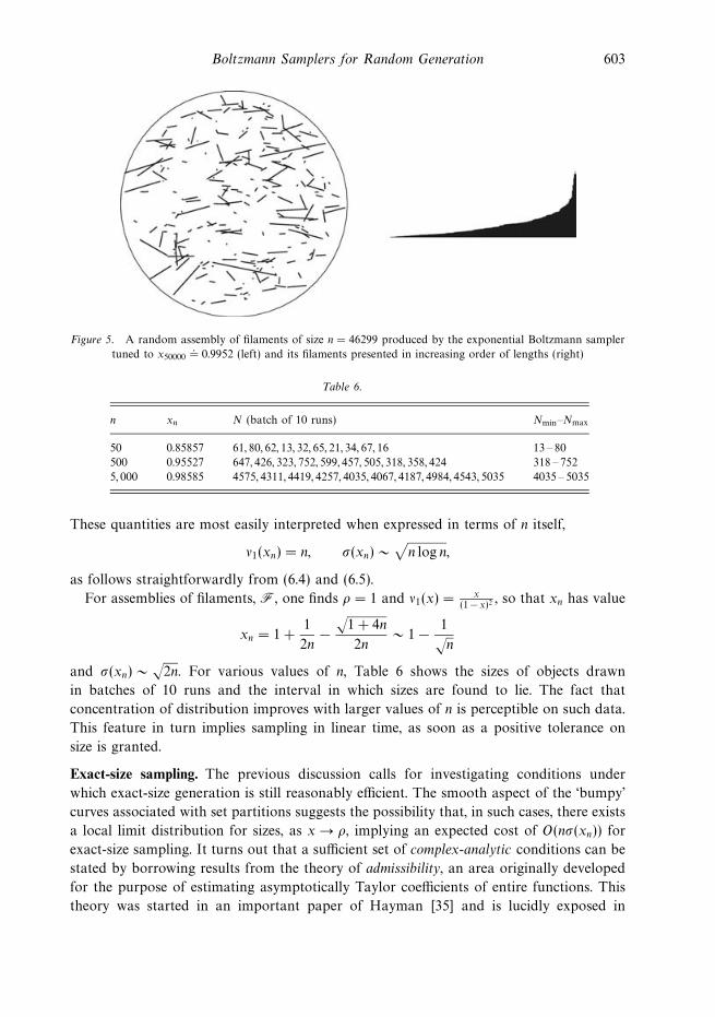
Table 6.
n xn N (batch of 10 runs) Nmin–Nmax
50 0.85857 61, 80, 62, 13, 32, 65, 21, 34, 67, 16 13 – 80
500 0.95527 647, 426, 323, 752, 599, 457, 505, 318, 358, 424 318 – 752
5, 000 0.98585 4575, 4311, 4419, 4257, 4035, 4067, 4187, 4984, 4543, 5035 4035 – 5035
These quantities are most easily interpreted when expressed in terms of n itself,
ν1(xn) = n, σ(xn) ∼√n log n,
as follows straightforwardly from (6.4) and (6.5).
For assemblies of filaments, F, one finds ρ = 1 and ν1(x) = x(1 − x)2 , so that xn has value
xn = 1 +1
2n−
√1 + 4n
2n∼ 1 − 1√
n
and σ(xn) ∼√
2n. For various values of n, Table 6 shows the sizes of objects drawn
in batches of 10 runs and the interval in which sizes are found to lie. The fact that
concentration of distribution improves with larger values of n is perceptible on such data.
This feature in turn implies sampling in linear time, as soon as a positive tolerance on
size is granted.
Exact-size sampling. The previous discussion calls for investigating conditions under
which exact-size generation is still reasonably efficient. The smooth aspect of the ‘bumpy’
curves associated with set partitions suggests the possibility that, in such cases, there exists
a local limit distribution for sizes, as x → ρ, implying an expected cost of O(nσ(xn)) for
exact-size sampling. It turns out that a sufficient set of complex-analytic conditions can be
stated by borrowing results from the theory of admissibility, an area originally developed
for the purpose of estimating asymptotically Taylor coefficients of entire functions. This
theory was started in an important paper of Hayman [35] and is lucidly exposed in
604 P. Duchon, P. Flajolet, G. Louchard and G. Schaeffer
Odlyzko’s survey [52, Section 12]. A function is said to be H-admissible if, in addition to
the mean value condition (6.1) and the variance condition (6.3), it satisfies the following
two properties.
• There exists a function δ(x) defined for x < ρ with 0 < δ(x) < π such that, for |θ| <δ(x) as x → ρ−,
f(xeiθ) ∼ f(x)eiaθ− 12 bθ
2
, a = ν1(x), b = σ2(x).
• Uniformly as x → ρ−, for δ(x) |θ| π,
f(xeiθ) = o
(f(x)
σ(x)
).
These conditions are the minimal ones that guarantee the applicability of the saddle-
point method to Cauchy coefficient integrals. They imply, in particular, knowledge of the
asymptotic form of the coefficients of f, namely,
fn ≡ [zn]f(z) ∼ f(xn)√2πxnnσ(xn)
, n → ∞.
We state the following.
Theorem 6.2. Consider a class C whose generating function f(z) satisfies the complex-
analytic conditions of H-admissibility. Then exact size rejection sampling based on µC(xn;
n, 0) succeeds in a mean number of trials that is asymptotic to√
2πσ(xn).
In particular, if C is specifiable, then the overall cost of exact-size sampling is O(nσ(xn)) on
average.
Proof. This is a direct adaptation of one of Hayman’s estimates, see Theorem I of [35]
(specialized in the notation of [35] as r → xn, n → m),
fmxmn
f(xn)∼ 1√
2πσ(xn)exp
(− (m− n)2
2σ(xn)2+ o(1)
),
uniformly for all m as xn → ρ. This last equation means generally that the distribution of
size values m is asymptotically normal as xn → ρ−, that is, as n → ∞. The specialization
m = n gives the statement.
Hayman admissibility is easily checked to be satisfied by the EGFs of set partitions and
assemblies of filaments. There results that exact size sampling has the following costs:
set partitions: O(n3/2√
log n); assemblies: O(n3/2).
Another result of Hayman states that, under H-admissibility, standard deviation is smaller
than the mean, σ(xn) = o(n) (see Corollary I of [35]), so that exact-size generation by
Boltzmann rejection is necessarily subquadratic (o(n2)).
The usefulness of Hayman’s conditions devolves from a rich set of closure properties:
under mild restrictions, admissible functions are closed under sum (f + g), product (fg),
Boltzmann Samplers for Random Generation 605
and exponentiation (ef). An informally stated consequence is then: For classes whose
generating function is ‘dominated’ by an exponential, i.e., the ‘principal’ construction is of the
set type, approximate-size generation is of linear time complexity and exact-size generation
is of subquadratic complexity. Here are a few more examples.
• Statistical classification theory superimposes a tree structure on objects based on a
similarity measure (e.g., the number of common phenotypes or genes). In this context,
the value of a proposed classification tree may be assessed by comparing it to a
random classification tree (structural properties should be substantially different in
order for the classification to be likely to make sense). Such comparisons in turn
benefit from random generation algorithms, a point originally made by Van Cutsem
and collaborators [63, 64]. For instance, hierarchies are labelled objects determined by
H = Z + P2(H),
and they correspond to Schroder’s systems of combinatorial theory [9, pp. 223–224].
Hierarchies with a bounded depth of nesting are of interest in this context, and their
EGFs
ez − 1, z + eez−1 − ez, ez+e
ez−1−ez − 1 − eez−1 + ez, . . . ,
are all admissible, hence amenable to the conclusions of Theorem 6.2.
• Similar comments apply to labelled trees (Cayley trees, T = Z P(T)) of bounded
height, with the sequence of EGFs starting as
z, zez, zezez
, zezezez
, . . . ,
and to ‘superpartitions’ obtained by iterating the construction P1:
eez−1 − 1, ee
ez−1−1 − 1, eeeez−1−1−1 − 1,
where, e.g., the number sequence (1, 3, 12, 60, 358, . . . ) associated to the second case is
A000258 of Sloane’s EIS [58]. Related structures are of interest in finite model theory;
see [68] for an introduction.
• Admissibility also covers generating functions of the type eP (z), with P a polynomial
with nonnegative coefficients. This includes permutations with sizes of cycles con-
strained to be in a finite set Ω, for instance involutions (I = P(C1,2(Z)), the solutions
of σd = Id in the symmetric group, and permutations whose longest cycle is at most
some fixed value m.
The conditions of Theorem 6.1 are not satisfied by words without long runs (Example 1),
surjections (Example 6, observe the lack of concentration on Figure 1, middle), and
permutations (Example 7), although they fail by little, since the mean and standard
deviation, ν1(x) and σ(x), happen to be of the same order of magnitude. They fail more
dramatically for binary trees (Example 2 and Figure 1, bottom), secondary structures
(Example 3), and non-crossing graphs (Example 4), where the ratio σ(x)/ν1(x) now tends
to infinity, in which case sizes produced by Boltzmann models exhibit a high dispersion.
As discussed in the next two subsections and in Section 7, such situations can, however,
be dealt with.
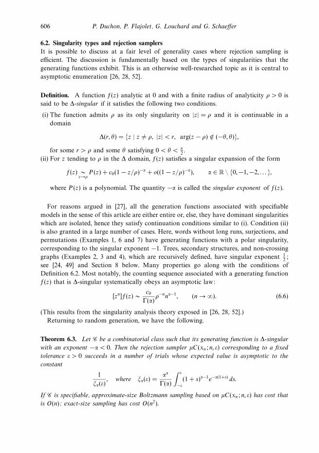
606 P. Duchon, P. Flajolet, G. Louchard and G. Schaeffer
6.2. Singularity types and rejection samplers
It is possible to discuss at a fair level of generality cases where rejection sampling is
efficient. The discussion is fundamentally based on the types of singularities that the
generating functions exhibit. This is an otherwise well-researched topic as it is central to
asymptotic enumeration [26, 28, 52].
Definition. A function f(z) analytic at 0 and with a finite radius of analyticity ρ > 0 is
said to be ∆-singular if it satisfies the following two conditions.
(i) The function admits ρ as its only singularity on |z| = ρ and it is continuable in a
domain
∆(r, θ) = z | z = ρ, |z| < r, arg(z − ρ) ∈ (−θ, θ),
for some r > ρ and some θ satisfying 0 < θ < π2.
(ii) For z tending to ρ in the ∆ domain, f(z) satisfies a singular expansion of the form
f(z) ∼z→ρ
P (z) + c0(1 − z/ρ)−α + o((1 − z/ρ)−α), α ∈ R \ 0,−1,−2, . . . ,
where P (z) is a polynomial. The quantity −α is called the singular exponent of f(z).
For reasons argued in [27], all the generation functions associated with specifiable
models in the sense of this article are either entire or, else, they have dominant singularities
which are isolated, hence they satisfy continuation conditions similar to (i). Condition (ii)
is also granted in a large number of cases. Here, words without long runs, surjections, and
permutations (Examples 1, 6 and 7) have generating functions with a polar singularity,
corresponding to the singular exponent −1. Trees, secondary structures, and non-crossing
graphs (Examples 2, 3 and 4), which are recursively defined, have singular exponent 12;
see [24, 49] and Section 8 below. Many properties go along with the conditions of
Definition 6.2. Most notably, the counting sequence associated with a generating function
f(z) that is ∆-singular systematically obeys an asymptotic law:
[zn]f(z) ∼ c0
Γ(α)ρ−nnα−1, (n → ∞). (6.6)
(This results from the singularity analysis theory exposed in [26, 28, 52].)
Returning to random generation, we have the following.
Theorem 6.3. Let C be a combinatorial class such that its generating function is ∆-singular
with an exponent −α < 0. Then the rejection sampler µC(xn; n, ε) corresponding to a fixed
tolerance ε > 0 succeeds in a number of trials whose expected value is asymptotic to the
constant
1
ξα(ε), where ξα(ε) =
αα
Γ(α)
∫ ε
−ε(1 + s)α−1e−α(1+s) ds.
If C is specifiable, approximate-size Boltzmann sampling based on µC(xn; n, ε) has cost that
is O(n); exact-size sampling has cost O(n2).
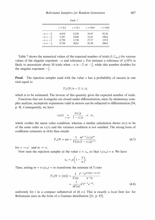
Boltzmann Samplers for Random Generation 607
Table 7.
ε = 0.2 ε = 0.1 ε = 0.05 ε = 0.01
−α = −2 4.619 9.236 18.47 92.36
−α = − 32 5.387 10.80 21.61 108.0
−α = −1 6.750 13.56 27.17 135.9
−α = − 12 9.236 20.61 41.30 206.6
Table 7 shows the numerical values of the expected number of trials (1/ξα(ε)) for various
values of the singular exponent −α and tolerance ε. For instance a tolerance of ±10% is
likely to necessitate about 10 trials when −α is −2 or − 32, while this number doubles for
the singular exponent − 12.
Proof. The rejection sampler used with the value x has a probability of success in one
trial equal to
Px(|N/n− 1| ε),
which is to be estimated. The inverse of this quantity gives the expected number of trials.
Functions that are ∆-singular are closed under differentiation, since, by elementary com-
plex analysis, asymptotic expansions valid in sectors can be subjected to differentiation [54,
p. 9]. Consequently, we have
ν1(x) ∼x→ρ−
αx/ρ
1 − x/ρ→ ∞,
which verifies the mean value condition, whereas a similar calculation shows σ(x) to be
of the same order as ν1(x) and the variance condition is not satisfied. The strong form of
coefficient estimates in (6.6) then entails
Px(N = m) ∼ 1
Γ(α)
mα−1|x/ρ|m(1 − x/ρ)−α , (6.7)
for x → ρ− and m → ∞.
Now tune the rejection sampler at the value x = xn, so that ν1(xn) = n. We have
xn ∼ ρ
(1 − α
n
).
Then, setting m = tν1(xn) = tn transforms the estimate (6.7) into
Px(N = tn) ∼ 1
Γ(α)
tα−1etn log(1−(α/n))
α−αn
∼ 1
nΓ(α)ααtα−1e−αt, (6.8)
uniformly for t in a compact subinterval of (0,∞). This is exactly a local limit law for
Boltzmann sizes in the form of a Gamma distribution [21, p. 47].
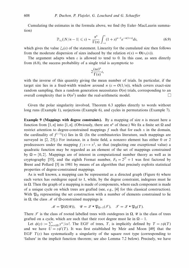
608 P. Duchon, P. Flajolet, G. Louchard and G. Schaeffer
Cumulating the estimates in the formula above, we find (by Euler–MacLaurin summa-
tion)
Pxn (|N/n− 1| ε) ∼ αα
Γ(α)
∫ ε
−ε(1 + s)α−1e−α(1+s)ds, (6.9)
which gives the value ξα(ε) of the statement. Linearity for the cumulated size then follows
from the moderate dispersion of sizes induced by the relation σ(x) = Θ(ν1(x)).
The argument adapts when ε is allowed to tend to 0. In this case, as seen directly
from (6.8), the success probability of a single trial is asymptotic to
2(αe)α
Γ(α)ε,
with the inverse of this quantity giving the mean number of trials. In particular, if the
target size lies in a fixed-width window around n (ε = O(1/n)), which covers exact-size
random sampling, then a random generation necessitates O(n) trials, corresponding to an
overall complexity that is O(n2) under the real-arithmetic model.
Given the polar singularity involved, Theorem 6.3 applies directly to words without
long runs (Example 1), surjections (Example 6), and cycles in permutations (Example 7).
Example 9 (Mappings with degree constraints). By a mapping of size n is meant here a
function from [1, n] into [1, n]. (Obviously, there are nn of these.) We fix a finite set Ω and
restrict attention to degree-constrained mappings f such that for each x in the domain,
the cardinality of f(−1)(x) lies in Ω. (In the combinatorics literature, such mappings are
surveyed in [2, 25].) For instance, in a finite field, a nonzero element has either 0 or 2
predecessors under the mapping f; x → x2, so that (neglecting one exceptional value) a
quadratic function may be regarded as an element of the set of mappings constrained
by Ω = 0, 2. Mappings are of interest in computational number theory as well as in
cryptography [55], and the eighth Fermat number, F8 = 228
+ 1 was first factored by
Brent and Pollard [5] in 1981 by means of an algorithm that precisely exploits statistical
properties of degree-constrained mappings.
As is well known, a mapping can be represented as a directed graph (Figure 6) where
each vertex has outdegree equal to 1, while, by the degree constraint, indegrees must lie
in Ω. Then the graph of a mapping is made of components, where each component is made
of a unique cycle on which trees are grafted (see, e.g., [4] for this classical construction).
With PΩ representing the set construction with a number of elements constrained to lie
in Ω, the class M of Ω-constrained mappings is
M = P(C(U)), U = Z PΩ−1(T), T = Z PΩ(T ).
There T is the class of rooted labelled trees with outdegrees in Ω, U is the class of trees
grafted on a cycle, which are such that their root degree must lie in Ω − 1.
Let φ(y) :=∑
ω∈Ω yω/ω!. The EGF of trees, T , is implicitly defined by T = zφ(T )
and we have U = zφ′(T ). It was first established by Meir and Moon [49] that the
EGF T (z) has systematically a singularity of the square root type (corresponding to
‘failure’ in the implicit function theorem; see also Lemma 7.2 below). Precisely, we have
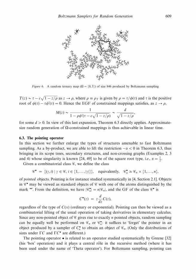
Boltzmann Samplers for Random Generation 609
Figure 6. A random ternary map (Ω = 0, 3) of size 846 produced by Boltzmann sampling
T (z) ∼ τ− c√
1 − z/ρ as z → ρ, where ρ ≡ ρT is given by ρ = τ/φ(τ) and τ is the positive
root of φ(τ) − τφ′(τ) = 0. Hence the EGF of constrained mappings satisfies, as z → ρ,
M(z) ∼ 1
1 − ρφ′(τ− c√
1 − z/ρ)∼ d√
1 − z/ρ,
for some d > 0. In view of this last expansion, Theorem 6.3 directly applies. Approximate-
size random generation of Ω-constrained mappings is thus achievable in linear time.
6.3. The pointing operator
In this section we further enlarge the types of structures amenable to fast Boltzmann
sampling. As a by-product, we are able to lift the restriction −α < 0 in Theorem 6.3, thus
bringing in its scope trees, secondary structures, and non-crossing graphs (Examples 2, 3
and 4) whose singularity is known [24, 49] to be of the square root type, i.e., α = 12.
Given a combinatorial class C, we define the class
C• = (γ, i) | γ ∈ C, i ∈ 1, . . . , |γ|, equivalently, C•n Cn × 1, . . . , n,
of pointed objects. Pointing is for instance studied systematically in [4, Section 2.1]. Objects
in C• may be viewed as standard objects of C with one of the atoms distinguished by the
mark ‘•’. From the definition, we have |C•n| = n|Cn|, and the GF of the class C• is
C•(z) = zd
dzC(z),
regardless of the type of C(x) (ordinary or exponential). Pointing can then be viewed as a
combinatorial lifting of the usual operation of taking derivatives in elementary calculus.
Since any non-pointed object of C gives rise to exactly n pointed objects, random sampling
can be equally well be performed on Cn or C•n: it suffices to ‘forget’ the pointer in an
object produced by a sampler of C•n to obtain an object of Cn. (Only the distributions of
sizes under ΓC and ΓC• are different.)
The pointing operator • is related to an operator studied systematically by Greene [32]
(his ‘box’ operation) and it plays a central role in the recursive method (where it has
been used under the name of ‘Theta operator’). For Boltzmann sampling, pointing can
610 P. Duchon, P. Flajolet, G. Louchard and G. Schaeffer
be used in conjunction with the previously defined operators +,× and ,S,P,C in either
the labelled or unlabelled universe.
Lemma 6.4. Let C be a specifiable unlabelled or labelled class (in the sense of Theorem 3.1
or 4.1). Then the class C• is also specifiable, i.e., it admits a specification without the pointing
operator •.
Proof. First, for a finite class C, the class C• is also finite and can be represented (and
sampled) explicitly. Next, the pointing operator admits composition rules with all the
other operators; in the labelled case, we have(A + B)• = A• + B•, (A B)• = A• B + A B•,
(SA)• = SA A• SA, (CA)• = A• SA,
(PA)• = A• PA.
(6.10)
In the unlabelled case, the first three rules apply, upon changing the labelled product ‘’
into the Cartesian product ‘×’. These rules are a combinatorial analogue of the usual
differentiation rules, and have a simple interpretation: e.g., pointing at a sequence ((SA)•)
implies pointing at a component (A•), which breaks the chain and individuates a left
(SA) and a right (SA) subsequence.
Consider now a specification of the class C = F1 in the form of a system,
S = Fi = Φi(Z; F1, . . . ,Fm), i = 1, . . . , m,
where Fi are auxiliary classes and the Φi are functional terms involving finite classes and
the standard operators (without pointing). Then, we can build a specification of the class
C• in the form of a derived system,
S′ = S ∪ F•i = Ψi(Z; F1, . . . ,Fm,F•
1, . . . ,F•m), i = 1, . . . , m,
where the functionals Ψi do not involve the pointing operator ‘•’: Ψi is obtained from Φ•i
by application of the derivation rules until the pointing operator is applied to variables
only. In the derived specification, each F•i is treated as a new variable, thereby leading to
a complete elimination of the pointing operator within constructions.
Our interest in pointing lies in the following two observations.
• If a class C has a generating function C(z) that is ∆-analytic with exponent −α, then
the generating function zC ′(z) of the class C• is also ∆-analytic and has an exponent
−α− 1, which is smaller.
• Uniform sampling in Cn is equivalent to uniform sampling in C•n. As a consequence,
the sampler µC•(x; n, ε) is a correct approximate-size sampler for the class C (upon
removing the mark).
Let µC•k(x; n, ε) denote the rejection sampler of the class derived from C by k successive
applications of the pointing operator. The last two observations immediately lead to an
extension of Theorem 6.3.
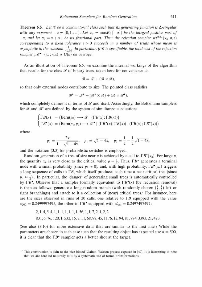
Boltzmann Samplers for Random Generation 611
Theorem 6.5. Let C be a combinatorial class such that its generating function is ∆-singular
with any exponent −α = 0, 1, . . . . Let α+ = max(0, −α) be the integral positive part of
−α, and let α0 = α+ α+ be its fractional part. Then the rejection sampler µC•α+(xn; n, ε)
corresponding to a fixed tolerance ε > 0 succeeds in a number of trials whose mean is
asymptotic to the constant 1ξα0 (ε)
. In particular, if C is specifiable, the total cost of the rejection
sampler µC•α+(xn; n, ε) is O(n) on average.
As an illustration of Theorem 6.5, we examine the internal workings of the algorithm
that results for the class B of binary trees, taken here for convenience as
B = Z + (B × B),
so that only external nodes contribute to size. The pointed class satisfies
B• = Z• + (B• × B) + (B × B•),
which completely defines it in terms of B and itself. Accordingly, the Boltzmann samplers
for B and B• are defined by the system of simultaneous equationsΓB(x) =
(Bern(p0) −→ Z | (ΓB(x); ΓB(x))
)ΓB•(x) =
(Bern(p1, p2) −→ Z• | (ΓB•(x); ΓB(x)) | (ΓB(x); ΓB•(x))
)where
p0 =2x
1 −√
1 − 4x, p1 =
√1 − 4x, p2 =
1
2− 1
2
√1 − 4x,
and the notation (3.3) for probabilistic switches is employed.
Random generation of a tree of size near n is achieved by a call to ΓB•(xn). For large n,
the quantity xn is very close to the critical value ρ = 14. Thus, ΓB• generates a terminal
node with a small probability (since p1 ≈ 0), and, with high probability, ΓB•(xn) triggers
a long sequence of calls to ΓB, which itself produces each time a near-critical tree (since
p0 ≈ 12) . In particular, the ‘danger’ of generating small trees is automatically controlled
by ΓB•. Observe that a sampler formally equivalent to ΓB•(x) (by recursion removal)
is then as follows: generate a long random branch (with randomly chosen ( 12, 1
2) left or
right branchings) and attach to it a collection of (near) critical trees.7 For instance, here
are the sizes observed in runs of 20 calls, one relative to ΓB equipped with the value
x500 = 0.2499997495, the other to ΓB• equipped with x′500 = 0.2497497497:
2, 1, 4, 5, 4, 1, 1, 1, 1, 1, 1, 1, 56, 1, 1, 7, 2, 1, 2, 2
831, 6, 76, 120, 1, 532, 15, 7, 11, 68, 99, 45, 1176, 12, 94, 81, 784, 3393, 21, 493.
(See also (3.10) for more extensive data that are similar to the first line.) While the
parameters are chosen in each case such that the resulting object has expected size n = 500,
it is clear that the ΓB• sampler gets a better shot at the target.
7 This construction is akin to the ‘size-biased’ Galton–Watson process exposed in [47]. It is interesting to note
that we are here led naturally to it by a systematic use of formal transformations.
612 P. Duchon, P. Flajolet, G. Louchard and G. Schaeffer
Pointing also constitutes a valuable optimization whenever structures are driven by a
cycle construction. Define a function f to be logarithmic if it is continuable in a ∆-domain
and satisfies
f(z) = c log1
1 − z/ρ+ O(1), z → ρ.
This may somehow be regarded as the limit case α → 0 of a singular exponent −α. As
Table 7 suggests, the efficiency of rejection deteriorates in this case: singularity analysis
may be used to verify that σ(xn) = n√
log n, so that approximate-size is of superlinear
complexity, namely O(n√
log n). This problem is readily fixed by pointing. If C = C(A),
then the transformation rules of (6.10) imply that we can alternatively generate a sequence,
which is amenable to straight rejection sampling in linear time, since its generating function
now has a polar-like singularity (with exponent −α = −1). For instance, the class K of
connected mappings is defined by
K = C(T), T = Z P(T).
The derived specification for K• is then
K• = T• S(T), T = Z P(T), T• = Z• P(T) + Z P(T) T•,
with non-terminals K•,T,T•. The generator ΓK• then achieves linear time sampling
for any fixed tolerance ε > 0. (Figure 6 has been similarly produced by pointing.)
This technique applies to plane trees and variants thereof (Example 2), secondary
structures (Example 3), and non-crossing graphs (Example 4). It also applies to all the
simple families of labelled nonplane trees, T = Z PΩ(T) defined by restrictions on
node degrees (Example 9). In all these cases, linear-time approximate-size sampling is
granted by Theorem 6.5.
7. Singular Boltzmann samplers
We now discuss two infinite categories of models, where it is possible to place oneself
right at the singularity x = ρC in order to develop rejection samplers from Boltzmann
models. These ‘singular’ rejection generators are freed from the necessity to adapt the
control variable x to the target size n, thus making available implementations that only
need a fixed set of constants to be determined once and for all, this independently of the
value of n.
7.1. Singular samplers for sequences
The first type of singular generator we present is dedicated to the sequence construction:
define a sequence construction to be supercritical if C = S(A) and ρA > ρC (so that
A(ρ−A ) > 1)). Put otherwise, the generating function of components A(x) should cross
the value 1 before it becomes singular. The generating functions of C and A satisfy
C(z) = 1/(1 − A(z)), so that the supercriticality condition implies that A(ρC) = 1 and the
(dominant) singularity ρC of C(x) is a pole. (This notion of supercriticality is borrowed
from Soria [59] who showed it to be determinant in the probabilistic properties of
sequences.)
Boltzmann Samplers for Random Generation 613
Literally taken, the Boltzmann sampler ΓC of Section 3 taken with x = ρC loops forever
and generates objects of infinite size, as it produces a number of components equal to
a ‘Geom(1)’. This prevents us from using the rejection algorithm µC(x; n, ε) with x = ρ.
However, one may adapt the idea by halting execution as soon as the target size has been
attained. Precisely, the early-interrupt singular sequence sampler is defined as follows:
function σC(ρ; n); Early-interrupt singular sequence sampleri := 0; repeat i := i+ 1; γi := ΓA(ρ) until |(γ1, . . . , γi)| > n;
return((γ1, . . . , γi)); end.
The principle of the algorithm can be depicted as ‘leapfrogging’ over n:
The singular early-interrupt sampler determined by the choice x = ρC has excellent prob-
abilistic and complexity-theoretic characteristics summarized in the following statement.
There, we assume without loss of generality that A(z) is aperiodic in the sense that the
quantity d := gcdn | An = 0 satisfies d = 1. (If d 2, a linear change of the size functions
brings us back to the aperiodic case.)
Theorem 7.1. Consider a sequence construction, C = S(A) that is supercritical and aperi-
odic. Then the early-interrupt singular sequence generator, σC(ρC ; n) is a valid sampler for C.
It produces an object of size n+ O(1) in one trial with high probability. For a specifiable
class A, exact-size random generation in C is achievable from this generator by rejection in
expected time O(n).
Proof. Let Xn denote the random variable giving the size of the output of the early-
interrupt singular sequence generator with target size n. The analysis of Xn can be treated
by classical renewal theory [20, Section XIII.10], but we opt for a direct approach based
on generating functions, which integrates smoothly within our general formalism.
The bivariate (probability) generating function with variable z marking the target size
n and variable u marking the size Xn of the actually generated object is
F(z, u) :=∑n1
∑mn
P(Xn = m) znum.
A trial decomposes into a sequence of samples of ΓA(ρ) ending by a sample that brings
the total over n, which implies
F(z, u) =1
1 − A(ρzu)L[A(ρzu)] =
z
1 − z
A(ρu) − A(ρzu)
1 − A(ρzu).
There L[f(z)] := z(f(1) − f(z))/(1 − z) is a linear operator, and, e.g.,
L[
1
1 − zu
]= z(u+ u2 + · · · ) + z2(u2 + u3 + · · · ) + z3(u3 + u4 + · · · ) + · · · ,
so that all powers of the form znu with n are produced.
614 P. Duchon, P. Flajolet, G. Louchard and G. Schaeffer
We check that F(z, 1) = z/(1 − z), as it should be. Next the expected size E(Xn) of the
output is given by the coefficient of zn in
∂
∂uF(z, u)|u=1 =
z
1 − z
ρA′(ρ)
1 − A(ρz)
=z
(1 − z)2+ρA′′(ρ)
2A′(ρ)· z
1 − z+ O(1) (z → 1).
This expansion at the polar singularity 1 then yields the expected ‘overshoot’:
E(Xn − n) = [zn]∂
∂uF(z, u)|u=1 − n =
ρA′′(ρ)
2A′(ρ)+ O(1/n).
The second moment of the expected size of the output is similarly obtained via two
successive differentiations. A simple computation then shows the variance of the overshoot
to satisfy
E((Xn − n)2) − E(Xn − n)2 = O(1).
As a matter of fact, the discrete distribution of the overshoot is described by
P(Xn − n = m) = [znun+m]F(z, u) = [znum]z
u− z
(1 − 1 − A(ρu)
1 − A(ρz)
),
= [zn+m]1
1 − A(ρz)−
m−1∑ =0
[zn+ ]1
1 − A(ρz)[um− ]A(ρu),
=
(1
ρA′(ρ)+ O(1/n)
)(1 −
m−1∑ =0
P(N = )
)
=P(N m)
E(N)+ O(1/n),
where N denotes the random size of an element of A under the Boltzmann model of
parameter ρ and the two last estimates hold for n → ∞ uniformly in m. The distribution
of N has exponential tails (since ρ ≡ ρC lies strictly within the disc of convergence of
A(z)), and thus the probability of a large overshoot decays geometrically fast. This proves
that exact size n is attained in O(1) trials.
This theorem applies to ‘cores’ of words without long runs (equation (3.9) from
Example 1) and it can be adapted to yield a generator of the full set R. It applies
to surjections (Example 6), for which exact-size generation becomes possible in linear
time. It also provides a global setting for a variety of ad hoc algorithms developed by
Louchard [43, 44, 46] in the context of efficient generation of certain types (directed,
convex) of random planar diagrams known as ‘animals’ and ‘polyominoes’.
Example 10 (Coin fountains (O)). A fountain is formed by starting with a row of coins,
then stacking additional coins on top so that each new coin touches two in the previous
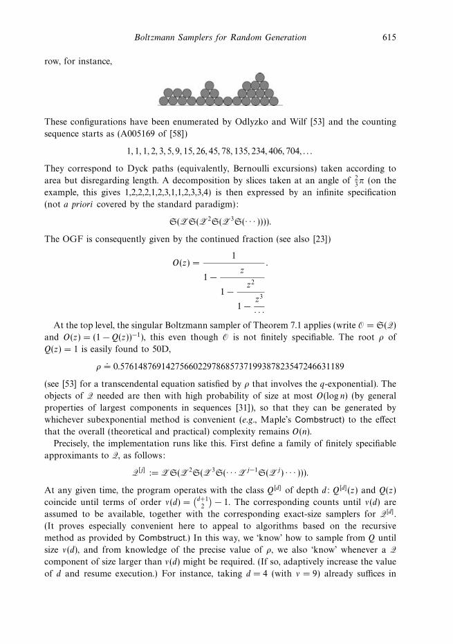
Boltzmann Samplers for Random Generation 615
row, for instance,
These configurations have been enumerated by Odlyzko and Wilf [53] and the counting
sequence starts as (A005169 of [58])
1, 1, 1, 2, 3, 5, 9, 15, 26, 45, 78, 135, 234, 406, 704, . . .
They correspond to Dyck paths (equivalently, Bernoulli excursions) taken according to
area but disregarding length. A decomposition by slices taken at an angle of 23π (on the
example, this gives 1,2,2,2,1,2,3,1,1,2,3,3,4) is then expressed by an infinite specification
(not a priori covered by the standard paradigm):
S(ZS(Z2S(Z3S(· · · )))).
The OGF is consequently given by the continued fraction (see also [23])
O(z) =1
1 −z
1 −z2
1 −z3
· · ·
.
At the top level, the singular Boltzmann sampler of Theorem 7.1 applies (write O = S(Q)
and O(z) = (1 − Q(z))−1), this even though O is not finitely specifiable. The root ρ of
Q(z) = 1 is easily found to 50D,
ρ.
= 0.5761487691427566022978685737199387823547246631189
(see [53] for a transcendental equation satisfied by ρ that involves the q-exponential). The
objects of Q needed are then with high probability of size at most O(log n) (by general
properties of largest components in sequences [31]), so that they can be generated by
whichever subexponential method is convenient (e.g., Maple’s Combstruct) to the effect
that the overall (theoretical and practical) complexity remains O(n).
Precisely, the implementation runs like this. First define a family of finitely specifiable
approximants to Q, as follows:
Q[j] := ZS(Z2S(Z3S(· · · Zj−1S(Zj) · · · ))).
At any given time, the program operates with the class Q[d] of depth d: Q[d](z) and Q(z)
coincide until terms of order ν(d) =(d+1
2
)− 1. The corresponding counts until ν(d) are
assumed to be available, together with the corresponding exact-size samplers for Q[d].
(It proves especially convenient here to appeal to algorithms based on the recursive
method as provided by Combstruct.) In this way, we ‘know’ how to sample from Q until
size ν(d), and from knowledge of the precise value of ρ, we also ‘know’ whenever a Qcomponent of size larger than ν(d) might be required. (If so, adaptively increase the value
of d and resume execution.) For instance, taking d = 4 (with ν = 9) already suffices in
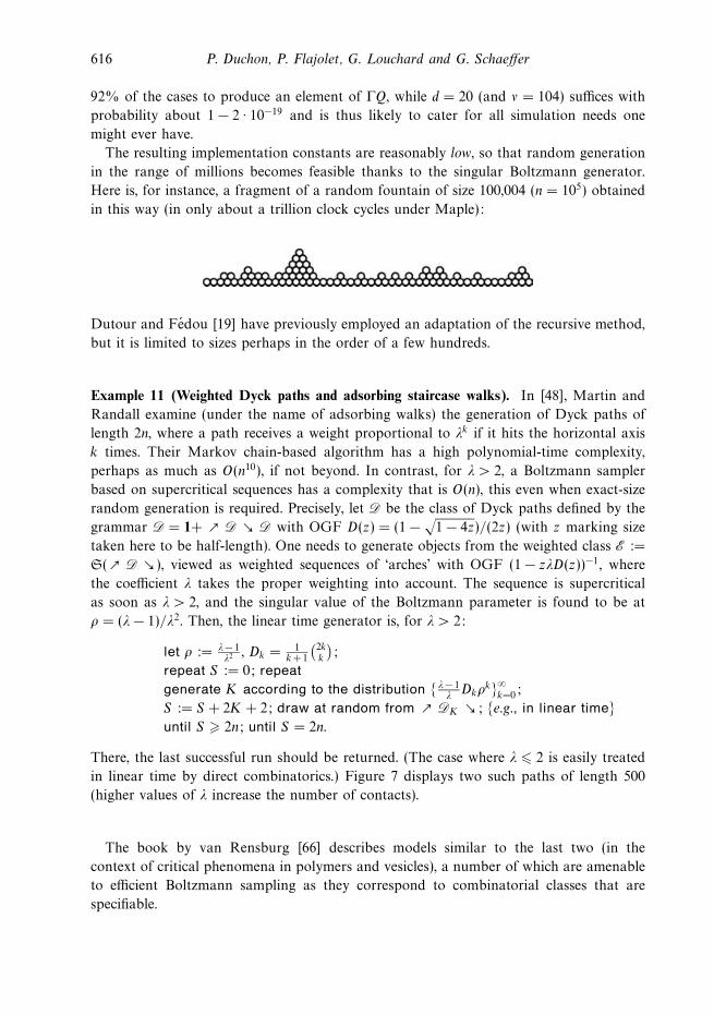
616 P. Duchon, P. Flajolet, G. Louchard and G. Schaeffer
92% of the cases to produce an element of ΓQ, while d = 20 (and ν = 104) suffices with
probability about 1 − 2 · 10−19 and is thus likely to cater for all simulation needs one
might ever have.
The resulting implementation constants are reasonably low, so that random generation
in the range of millions becomes feasible thanks to the singular Boltzmann generator.
Here is, for instance, a fragment of a random fountain of size 100,004 (n = 105) obtained
in this way (in only about a trillion clock cycles under Maple):
Dutour and Fedou [19] have previously employed an adaptation of the recursive method,
but it is limited to sizes perhaps in the order of a few hundreds.
Example 11 (Weighted Dyck paths and adsorbing staircase walks). In [48], Martin and
Randall examine (under the name of adsorbing walks) the generation of Dyck paths of
length 2n, where a path receives a weight proportional to λk if it hits the horizontal axis
k times. Their Markov chain-based algorithm has a high polynomial-time complexity,
perhaps as much as O(n10), if not beyond. In contrast, for λ > 2, a Boltzmann sampler
based on supercritical sequences has a complexity that is O(n), this even when exact-size
random generation is required. Precisely, let D be the class of Dyck paths defined by the
grammar D = 1+ D D with OGF D(z) = (1 −√
1 − 4z)/(2z) (with z marking size
taken here to be half-length). One needs to generate objects from the weighted class E :=
S( D ), viewed as weighted sequences of ‘arches’ with OGF (1 − zλD(z))−1, where
the coefficient λ takes the proper weighting into account. The sequence is supercritical
as soon as λ > 2, and the singular value of the Boltzmann parameter is found to be at
ρ = (λ− 1)/λ2. Then, the linear time generator is, for λ > 2:
let ρ := λ− 1λ2 , Dk = 1
k+ 1
(2kk
);
repeat S := 0; repeat
generate K according to the distribution λ− 1λDkρ
k∞k=0;
S := S + 2K + 2; draw at random from DK ; e.g., in linear timeuntil S 2n; until S = 2n.
There, the last successful run should be returned. (The case where λ 2 is easily treated
in linear time by direct combinatorics.) Figure 7 displays two such paths of length 500
(higher values of λ increase the number of contacts).
The book by van Rensburg [66] describes models similar to the last two (in the
context of critical phenomena in polymers and vesicles), a number of which are amenable
to efficient Boltzmann sampling as they correspond to combinatorial classes that are
specifiable.
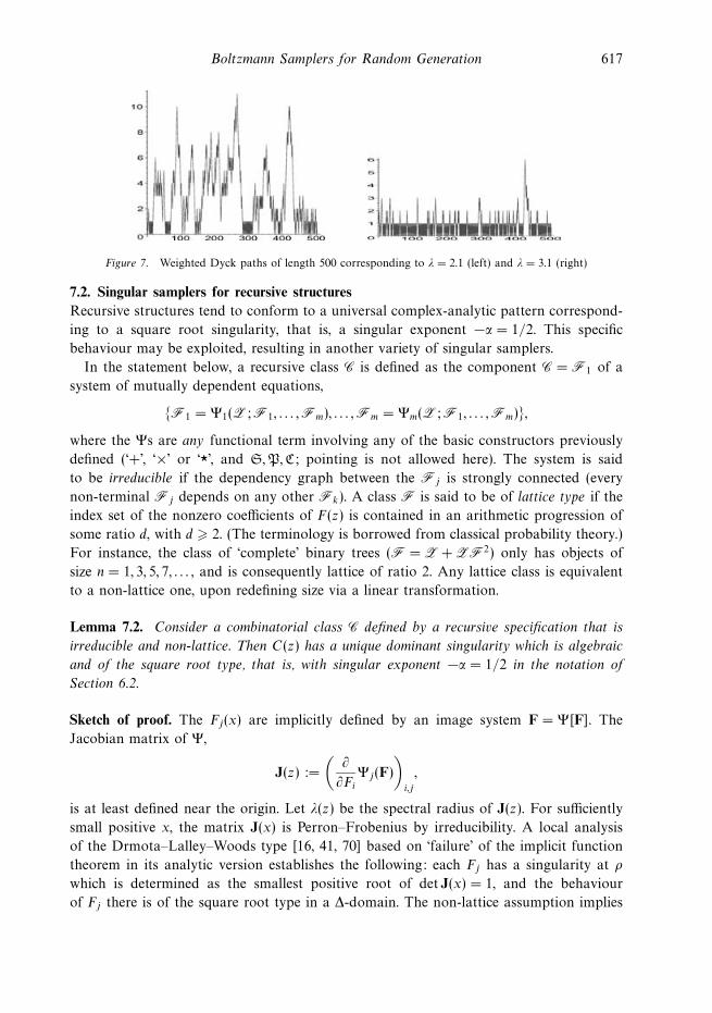
Boltzmann Samplers for Random Generation 617
Figure 7. Weighted Dyck paths of length 500 corresponding to λ = 2.1 (left) and λ = 3.1 (right)
7.2. Singular samplers for recursive structures
Recursive structures tend to conform to a universal complex-analytic pattern correspond-
ing to a square root singularity, that is, a singular exponent −α = 1/2. This specific
behaviour may be exploited, resulting in another variety of singular samplers.
In the statement below, a recursive class C is defined as the component C = F1 of a
system of mutually dependent equations,
F1 = Ψ1(Z; F1, . . . ,Fm), . . . ,Fm = Ψm(Z; F1, . . . ,Fm),
where the Ψs are any functional term involving any of the basic constructors previously
defined (‘+’, ‘×’ or ‘’, and S,P,C; pointing is not allowed here). The system is said
to be irreducible if the dependency graph between the Fj is strongly connected (every
non-terminal Fj depends on any other Fk). A class F is said to be of lattice type if the
index set of the nonzero coefficients of F(z) is contained in an arithmetic progression of
some ratio d, with d 2. (The terminology is borrowed from classical probability theory.)
For instance, the class of ‘complete’ binary trees (F = Z + ZF2) only has objects of
size n = 1, 3, 5, 7, . . . , and is consequently lattice of ratio 2. Any lattice class is equivalent
to a non-lattice one, upon redefining size via a linear transformation.
Lemma 7.2. Consider a combinatorial class C defined by a recursive specification that is
irreducible and non-lattice. Then C(z) has a unique dominant singularity which is algebraic
and of the square root type, that is, with singular exponent −α = 1/2 in the notation of
Section 6.2.
Sketch of proof. The Fj(x) are implicitly defined by an image system F = Ψ[F]. The
Jacobian matrix of Ψ,
J(z) :=
(∂
∂FiΨj(F)
)i,j
,
is at least defined near the origin. Let λ(z) be the spectral radius of J(z). For sufficiently
small positive x, the matrix J(x) is Perron–Frobenius by irreducibility. A local analysis
of the Drmota–Lalley–Woods type [16, 41, 70] based on ‘failure’ of the implicit function
theorem in its analytic version establishes the following: each Fj has a singularity at ρ
which is determined as the smallest positive root of det J(x) = 1, and the behaviour
of Fj there is of the square root type in a ∆-domain. The non-lattice assumption implies
618 P. Duchon, P. Flajolet, G. Louchard and G. Schaeffer
that each Fj satisfies |F(z)| < F(|z|) for any z satisfying 0 < |z| < ρ and z ∈ R>0; by
domination properties of analytic functions with positive coefficients and matrices with
complex entries, this implies that λ(z) < λ(|z|), whence the fact that each Fj is analytic on
|z| = ρ, z = ρ.
In view of Lemma 7.2, C(z) is ∆-singular with an expansion of the form
C(z) = C(ρ) − c0(1 − z/ρ)1/2 + O(1 − z/ρ), (7.1)
where C(ρ) > 0 and c0 > 0. Singularity analysis then implies that the coefficients are
asymptotically given by
[zn]C(z) =c0
2√πρ−nn−3/2(1 + O(n−1)). (7.2)
(For details see [28, Chapter 8] and reference therein.) Consequently, the distribution of
sizes at the critical value x = ρ is of the form P(N = n) ∝ n−3/2, which means that it has
heavy tails. In particular, the expectation of size E(N) is infinite (this fact is well known
in the special case of critical branching processes). Such an observation precludes the use
of straight-rejection Boltzmann sampling.
The idea of an early interruption discussed in the previous section may be adapted and
extended. Consider in all generality a Boltzmann sampler ΓC(x) built according to the
design principles already exposed and let m be a ceiling (i.e., an upper bound) imposed on
the size of the required objects. It is possible to build a modification ΓC<m(x) of ΓC(x)
as follows: maintain a running count, implemented as a global counter K , of the number
of atoms produced at any given time during a partial execution of sampling by ΓC(x);
the counter is regularly incremented as long as K m each time an atom is produced;
however, as soon as K exceeds m, execution is interrupted and the ‘undefined’ symbol ⊥is returned. Then, rejection can be piled on top of this sampler, which corresponds to the
scheme:
function νC(x; n, ε); Ceiled rejection samplerrepeat γ := ΓC<m(x; n(1 + ε)) until (γ =⊥) ∧ (|γ| n(1 − ε));
return(γ); end.
This ceiling technique optimizes any Boltzmann sampler for any value of x. The choice
of the singular value x = ρ makes the algorithm well-behaved for recursive classes.
Theorem 7.3. Let C be a combinatorial class given by a recursive specification that is irre-
ducible and aperiodic. Then the singular ceiled rejection sampler νC(ρ; n, ε), corresponding
to a fixed tolerance ε > 0 succeeds in a number of trials whose expected value grows like
n1/2/ζ(ε) for a positive constant ζ(ε) given by (7.5) below.
Moreover, the cumulated size Tn of the generated and rejected objects during the call of
νC(ρ; n, ε) satisfies, as n → ∞,
E(Tn) ∼ n
ε
((1 − ε)1/2 + (1 + ε)1/2
)(7.3)
Boltzmann Samplers for Random Generation 619
with its variance, σ2 = E(T 2n ) − E(Tn)
2, being
σ2 ∼ E(Tn)2 +
n2
ε
(1
3(1 − ε)3/2 + (1 + ε)3/2
). (7.4)
Under these conditions, approximate-size sampling and exact-size sampling are of average-
case complexity respectively O(n) and O(n2).
Proof. Let C(x) be the generating function of C, and let C<n1 (x), C>n2 (x), C [n1 ,n2](x) be
the generating function for the subclass of those objects with size respectively strictly
less than n1 = (1 − ε)n, strictly greater than n2 = (1 + ε)n, and between n1 and n2. The
coefficients of C(z) are known from equation (7.2), so that ΓC(ρ) produces sizes according
to
P(N = k) ∼ c0
2C(ρ)√πk−3/2.
For any ε > 0, the probability that a single trial (one execution of the repeat loop) of the
ceiled rejection sampler νC(ρ; n, ε) succeeds is obtained by summing over all values of k
in the interval [n(1 − ε), n(1 + ε)]. This probability thus decays like ζ(ε)n−1/2, where
ζ(ε) =c0
5C(ρ)√π
((1 + ε)5/2 − (1 − ε)5/2). (7.5)
The expected number of trials follows.
Next, the probability generating function of the interruptive singular Boltzmann sampler
targeted at [n1, n2] is
F(u) =∑k
P(Tn = k) uk.
From the decomposition of a call to νC into a sequence of unsuccessful trials (contributing
to Tn) followed by a final successful trial (not contributing to Tn),
F(u) =
(1 − 1
C(ρ)(C<n1 (ρu) + C>n2 (ρ)un2 )
)−1C [n1 ,n2](ρ)
C(ρ).
(This is the cost in addition to the size of the last successful output, and it is assumed that
the generation of objects with size larger than n2 is interrupted at size n2.) The moments
of the cost are then given by
E(Tn) =∂
∂uF(u)|u=1, E(T 2
n ) =(u∂)2
∂u2F(u)|u=1.
Taking partial derivatives, then specializing to u = 1, and observing that C(x) − C<n1 (x) −C>n2 (x) = C [n1 ,n2](x), we get
E(Tn) =ρC ′<n1 (ρ) + n2C
>n2 (ρ)
C [n1 ,n2](ρ),
E(T 2n ) =
ρ2C ′′<n1 (ρ) + n2(n2 − 1)C>n2 (ρ)
C [n1 ,n2](ρ)+ 2 E(Tn)
2 + E(Tn).
620 P. Duchon, P. Flajolet, G. Louchard and G. Schaeffer
The asymptotic expression for the coefficients of C(x) as given in (7.2) yields, by direct
Euler–MacLaurin summation:
ρC ′<n1 (ρ) ∼ 2c0n1/21 , ρ2C ′′<n1 (ρ) ∼ 2c0
3n
3/21 ,
C>n2 (ρ) ∼ 2c0n−1/22 , C [n1 ,n2](ρ) ∼ 2c0εn
−1/2. (7.6)
The estimates (7.6) combine with the exact expressions of E(Tn) and E(T 2n ) to give the
values stated in (7.3) and (7.4).
For a relative tolerance ε = εn depending on n and tending to zero, the estimates become
E(Tn) ∼ 2nε
and σ ∼ E(Tn), which implies the quadratic cost of exact-size sampling.
The singular ceiled rejection sampler thus provides linear-time approximate-size random
generation for all the simple varieties of trees of Example 2, including binary trees, unary-
binary trees, 2–3 trees, and so on, for secondary structures (Example 3), and for non-
crossing graphs (Example 4). In all these cases, exact-size is also achievable in quadratic
time. The method does not require the pointing transformations of Section 6.3 and only
necessitates a fixed number of constants, themselves independent of the target value n.
The technique is akin to the ‘Florentine algorithm’ invented by Barcucci, Pinzani and
Sprugnoli [3] to generate prefixes of Motzkin words and some directed plane animals.
The cost analysis given above is related to Louchard’s work [45].
Note. Let T be a class of trees determined by restricting the degrees of nodes to
lie in a finite set Ω, that is, T = SΩ(T) or T = PΩ(T), depending on whether the
trees are embedded in the plane or not. The corresponding generating function satisfies
T (z) = zφ(T (z)) (see Example 9). For such trees, exact-size sampling can be performed in
time O(n3/2), as we now explain – this improves on the general bound O(n2) of Theorem 7.3.
Indeed, in order to generate a tree of size n, it suffices to generate a Lukasiewicz code of
length n, with steps in Ω − 1. By Raney’s conjugacy principle [42, Chapter 11] (also known
as Dvoretzky and Motzkin’s cycle lemma), this task itself reduces to generating at random
a lattice path of length n with steps in Ω − 1 and with final altitude −1. When one places
oneself right at the singular value ρ (for T (z)), the latter task is equivalent to sampling
from n independent random variables, having support Ω − 1 and probability generating
function ψ(z) = φ(ρz)/(zφ(ρ)), and conditioned to sum to the value −1. Rejection (on the
final value of the n-sum) achieves this in O(n1/2) trials, by virtue of the local limit theorem
for sums of discrete random variables. In this way, trees from any finitely generated family
of trees can be sampled in total time O(n3/2); equivalently, the technique makes it possible
to sample from any branching process (with finitely supported offspring distribution)
conditioned upon the size of the total progeny being n, this again in time O(n3/2).
8. Conclusions
As shown here, combinatorial decompositions allow for random generation in low
polynomial time. In particular, approximate-size random generation can often be effected
in linear time, using algorithms that suitably exploit the ‘physics’ of random combinatorial
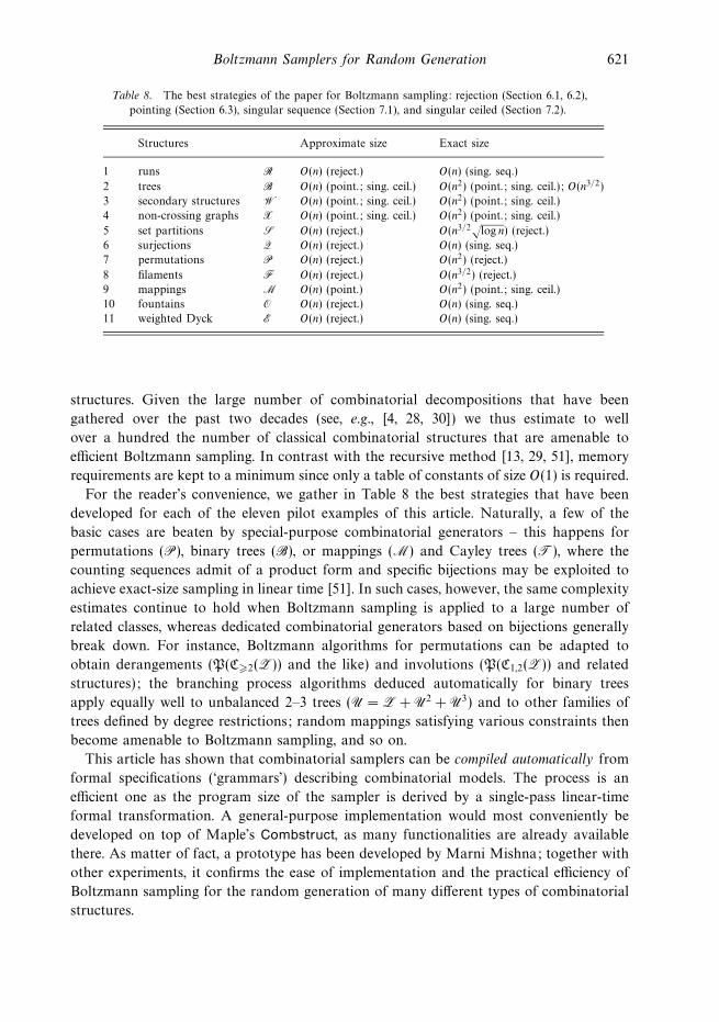
Boltzmann Samplers for Random Generation 621
Table 8. The best strategies of the paper for Boltzmann sampling: rejection (Section 6.1, 6.2),
pointing (Section 6.3), singular sequence (Section 7.1), and singular ceiled (Section 7.2).
Structures Approximate size Exact size
1 runs R O(n) (reject.) O(n) (sing. seq.)
2 trees B O(n) (point.; sing. ceil.) O(n2) (point.; sing. ceil.); O(n3/2)
3 secondary structures W O(n) (point.; sing. ceil.) O(n2) (point.; sing. ceil.)
4 non-crossing graphs X O(n) (point.; sing. ceil.) O(n2) (point.; sing. ceil.)
5 set partitions S O(n) (reject.) O(n3/2√
log n) (reject.)
6 surjections Q O(n) (reject.) O(n) (sing. seq.)
7 permutations P O(n) (reject.) O(n2) (reject.)
8 filaments F O(n) (reject.) O(n3/2) (reject.)
9 mappings M O(n) (point.) O(n2) (point.; sing. ceil.)
10 fountains O O(n) (reject.) O(n) (sing. seq.)
11 weighted Dyck E O(n) (reject.) O(n) (sing. seq.)
structures. Given the large number of combinatorial decompositions that have been
gathered over the past two decades (see, e.g., [4, 28, 30]) we thus estimate to well
over a hundred the number of classical combinatorial structures that are amenable to
efficient Boltzmann sampling. In contrast with the recursive method [13, 29, 51], memory
requirements are kept to a minimum since only a table of constants of size O(1) is required.
For the reader’s convenience, we gather in Table 8 the best strategies that have been
developed for each of the eleven pilot examples of this article. Naturally, a few of the
basic cases are beaten by special-purpose combinatorial generators – this happens for
permutations (P), binary trees (B), or mappings (M) and Cayley trees (T), where the
counting sequences admit of a product form and specific bijections may be exploited to
achieve exact-size sampling in linear time [51]. In such cases, however, the same complexity
estimates continue to hold when Boltzmann sampling is applied to a large number of
related classes, whereas dedicated combinatorial generators based on bijections generally
break down. For instance, Boltzmann algorithms for permutations can be adapted to
obtain derangements (P(C2(Z)) and the like) and involutions (P(C1,2(Z)) and related
structures); the branching process algorithms deduced automatically for binary trees
apply equally well to unbalanced 2–3 trees (U = Z + U2 + U3) and to other families of
trees defined by degree restrictions; random mappings satisfying various constraints then
become amenable to Boltzmann sampling, and so on.
This article has shown that combinatorial samplers can be compiled automatically from
formal specifications (‘grammars’) describing combinatorial models. The process is an
efficient one as the program size of the sampler is derived by a single-pass linear-time
formal transformation. A general-purpose implementation would most conveniently be
developed on top of Maple’s Combstruct, as many functionalities are already available
there. As matter of fact, a prototype has been developed by Marni Mishna; together with
other experiments, it confirms the ease of implementation and the practical efficiency of
Boltzmann sampling for the random generation of many different types of combinatorial
structures.
622 P. Duchon, P. Flajolet, G. Louchard and G. Schaeffer
In forthcoming works, we propose to demonstrate the versatility of Boltzmann sampling
for a number of simulation needs including:
• the extension of the set of allowed constructions, e.g., in the unlabelled case, sampling
for multisets (M, repetitions are allowed), powersets (P, no repetitions allowed), cycles
(C), and the substitution operation;
• multivariate extensions, meaning the sampling of configurations according to a
constraint on size and on an auxiliary parameter (e.g., words of some length containing
an unusual number of occurrences of a designated pattern);
• the realization of Boltzmann samplers using only discrete sources of randomness and
basic logical operations in the style of Knuth and Yao’s fundamental study [40] –
nearly linear Boolean (bit level) complexity still seems to be achievable in many cases
of practical interest.
Acknowledgements
The authors are grateful to Alain Denise, Bernard Ycart, Brigitte Vallee, Jim Fill,
Marni Mishna, Paul Zimmermann, and Philippe Robert for bibliographical suggestions,
programming ideas, as well as encouragements and architectural remarks. This work
was supported in part by the Alcom–FT Project IST-1999-14186 and by the IHRP
Programme (grant HPRN-CT-2001-00272: Algebraic Combinatorics in Europe) of the
European Union. Merci also to Gilles Kahn and INRIA for backing the Alcophys
Action under which some of these ideas were hatched and to CNRS (Gdr Alp and
Department Stic) for its sustained support of the French Group Alea. Grazie mille finally
to Alberto del Lungo and Renzo Pinzani for kindly offering an occasion to expose an
early form of these ideas at the Gascom meeting, Siena, November 2001.
References
[1] Aho, A. V. and Corasick, M. J. (1975) Efficient string matching: An aid to bibliographic search.
Comm. Assoc. Comput. Mach. 18 333–340.
[2] Arney, J. and Bender, E. D. (1982) Random mappings with constraints on coalescence and
number of origins. Pacific J Math. 103 269–294.
[3] Barcucci, E., Pinzani, R. and Sprugnoli, R. (1994) The random generation of directed animals.
Theoret. Comput. Sci. 127 333–350.
[4] Bergeron, F., Labelle, G. and Leroux, P. (1998) Combinatorial Species and Tree-Like Structures,
Cambridge University Press, Cambridge.
[5] Brent, R. P. and Pollard, J. M. (1981) Factorization of the eighth Fermat number. Math. Comp.
36 627–630.
[6] Burris, S. N. (2001) Number Theoretic Density and Logical Limit Laws, Vol. 86 of Mathematical
Surveys and Monographs, AMS, Providence, RI.
[7] Compton, K. J. (1987) A logical approach to asymptotic combinatorics I: First order properties.
Adv. Math. 65 65–96.
[8] Compton, K. J. (1987) A logical approach to asymptotic combinatorics II: Second–order
properties. J. Combin. Theory Ser. A 50 110–131.
[9] Comtet, L. (1974) Advanced Combinatorics, Reidel, Dordrecht.
[10] Dembo, A., Vershik, A. and Zeitouni, O. (2000) Large deviations for integer partitions. Markov
Process. Related Fields 6 147–179.
[11] den Hollander, F. (2000) Large Deviations, AMS, Providence, RI.
Boltzmann Samplers for Random Generation 623
[12] Denise, A., Dutour, I. and Zimmermann, P. (1998) CS: a MuPAD package for counting and
randomly generating combinatorial structures. In Proc. 10th Conference on Formal Power Series
and Algebraic Combinatorics, FPSAC’98 , pp. 195–204.
[13] Denise, A. and Zimmermann, P. (1999) Uniform random generation of decomposable structures
using floating-point arithmetic. Theoret. Comput. Sci. 218 233–248.
[14] Devroye, L. (1986) Non-Uniform Random Variate Generation, Springer.
[15] Domb, C. and Barrett, A. (1974) Enumeration of ladder graphs. Discrete Math. 9 341–358.
[16] Drmota, M. (1997) Systems of functional equations. Random Struct. Alg. 10 103–124.
[17] Duchon, P. (2001) Relaxed random generation of trees. Algorithms Seminar, 05-11-01.
[18] Duchon, P., Flajolet, P., Louchard, G. and Schaeffer, G. (2002) Random sampling from
Boltzmann principles. In Automata, Languages, and Programming, 2002 (P. Widmayer et al.,
eds), Vol. 2380 of Lecture Notes in Computer Science, Springer, pp. 501–513.
[19] Dutour, I. and Fedou, J.-M. (1998) Object grammars and random generation. Discrete Math.
Theor. Comput. Sci. 2 47–61.
[20] Feller, W. (1968) An Introduction to Probability Theory and its Applications, 3rd edn, Vol. 1,
Wiley.
[21] Feller, W. (1971) An Introduction to Probability Theory and its Applications, Vol. 2, Wiley.
[22] Fill, J. A. and Huber, M. (2000) The randomness recycler: A new technique for perfect sampling.
In Proc. 41th Annual IEEE Symposium on Foundations of Computer Science, 2000, pp. 503–
511.
[23] Flajolet, P. (1980) Combinatorial aspects of continued fractions. Discrete Math. 32 125–161.
[24] Flajolet, P. and Noy, M. (1999) Analytic combinatorics of non-crossing configurations. Discrete
Math. (selected papers in honour of Henry W. Gould) 204 203–229.
[25] Flajolet, P. and Odlyzko, A. M. (1990) Random mapping statistics. In Advances in Cryptology:
Proc. Eurocrypt’89, Houtalen, Belgium, April 1989 (J.-J. Quisquater and J. Vandewalle, eds),
Vol. 434 of Lecture Notes in Computer Science, Springer, pp. 329–354. .
[26] Flajolet, P. and Odlyzko, A. M. (1990) Singularity analysis of generating functions. SIAM J.
Algebraic Discrete Methods 3 216–240.
[27] Flajolet, P., Salvy, B. and Zimmermann, P. (1991) Automatic average-case analysis of algorithms.
Theoret. Comput. Sci. 79 37–109.
[28] Flajolet, P. and Sedgewick, R. (2001) Analytic Combinatorics, book in preparation: Individual
chapters are available as INRIA Research Reports 1888, 2026, 2376, 2956, 3162, 4103 and
electronically from http://algo.inria.fr/flajolet/Publications/books.html.
[29] Flajolet, P., Zimmerman, P. and Van Cutsem, B. (1994) A calculus for the random generation
of labelled combinatorial structures. Theoret. Comput. Sci. 132 1–35.
[30] Goulden, I. P. and Jackson, D. M. (1983) Combinatorial Enumeration, Wiley, New York.
[31] Gourdon, X. (1998) Largest component in random combinatorial structures. Discrete Math.
180 185–209.
[32] Greene, D. H. (1983) Labelled formal languages and their uses. PhD thesis, Stanford University.
Available as Report STAN-CS-83-982.
[33] Greene, D. H. and Knuth, D. E. (1981) Mathematics for the Analysis of Algorithms, Birkhauser,
Boston.
[34] Harary, F. and Palmer, E. M. (1973) Graphical Enumeration, Academic Press.
[35] Hayman, W. K. (1956) A generalization of Stirling’s formula. J. Reine Angew. Math. 196 67–95.
[36] Howell, J. A., Smith, T. F. and Waterman, M. S. (1980) Computation of generating functions
for biological molecules. SIAM J. Appl. Math. 39 119–133.
[37] Huang, K. (1987) Statistical Mechanics, 2nd edn, Wiley.
[38] Johnson, N. L. and Kotz, S. (1969) Discrete Distributions, Wiley.
[39] Knuth, D. E. (1998) The Art of Computer Programming, 3rd edn, Vol. 2, Seminumerical
Algorithms, Addison-Wesley.
624 P. Duchon, P. Flajolet, G. Louchard and G. Schaeffer
[40] Knuth, D. E. and Yao, A. C. (1976) The complexity of nonuniform random number generation.
In Algorithms and Complexity: Proc. Sympos., Carnegie-Mellon Univ., Pittsburgh, PA, 1976 ,
Academic Press, New York, pp. 357–428.
[41] Lalley, S. P. (1993) Finite range random walk on free groups and homogeneous trees. Ann.
Probab. 21 2087–2130.
[42] Lothaire, M. (1983) Combinatorics on Words, Vol. 17 of Encyclopedia of Mathematics and its
Applications, Addison-Wesley.
[43] Louchard, G. (1996) Probabilistic analysis of some (un)directed animals. Theoret. Comput. Sci.
159 65–79.
[44] Louchard, G. (1997) Probabilistic analysis of column-convex and directed diagonally-convex
animals. Random Struct. Alg. 11 151–178.
[45] Louchard, G. (1999) Asymptotic properties of some underdiagonal walks generation algorithms.
Theoret. Comput. Sci. 218 249–262.
[46] Louchard, G. (1999) Probabilistic analysis of column-convex and directed diagonally-convex
animals II: Trajectories and shapes. Random Struct. Alg. 15 1–23.
[47] Lyons, R., Pemantle, R. and Peres, Y. (1995) Conceptual proofs of L logL criteria for mean
behavior of branching processes. Ann. Probab. 23 1125–1138.
[48] Martin, R. and Randall, D. (2000) Sampling adsorbing staircase walks using a new Markov
chain decomposition method. In Proc. 41st Annual IEEE Symposium on Foundations of Computer
Science, FOCS 2000 , pp. 492–502.
[49] Meir, A. and Moon, J. W. (1978) On the altitude of nodes in random trees. Canad. J. Math. 30
997–1015.
[50] Milenkovic, O. and Compton, K. J. (2002) Probabilistic transforms for combinatorial urn
models. Combin. Probab. Comput. 13 XX–XX.
[51] Nijenhuis, A. and Wilf, H. S. (1978) Combinatorial Algorithms, 2nd edn, Academic Press.
[52] Odlyzko, A. M. (1995) Asymptotic enumeration methods. In Handbook of Combinatorics
(R. Graham, M. Grotschel and L. Lovasz, eds), Vol. II, Elsevier, Amsterdam, pp. 1063–1229.
[53] Odlyzko, A. M. and Wilf, H. S. (1988) The editor’s corner: n coins in a fountain. Amer. Math.
Monthly 95 840–843.
[54] Olver, F. W. J. (1974) Asymptotics and Special Functions, Academic Press.
[55] Quisquater, J.-J. and Delescaille, J.-P. (1990) How easy is collision search? Application to
DES. In Proc. EUROCRYPT’89 , Vol. 434 of Lecture Notes in Computer Science, Springer,
pp. 429–434.
[56] Schaeffer, G. (1999) Random sampling of large planar maps and convex polyhedra. In Proc.
31st Annual ACM Symposium on Theory of Computing, STOC’99; Atlanta, Georgia, May 1999,
ACM press, pp. 760–769.
[57] Shepp, L. A. and Lloyd, S. P. (1966) Ordered cycle lengths in a random permutation. Trans.
Amer. Math. Soc. 121 340–357.
[58] Sloane, N. J. A. (2000) The On-Line Encyclopedia of Integer Sequences. Published electronically
at http://www.research.att.com/~njas/sequences/.
[59] Soria-Cousineau, M. (1990) Methodes d’analyse pour les constructions combinatoires et les
algorithmes. Doctorat es sciences, Universite de Paris–Sud, Orsay.
[60] Stanley, R. P. (1986) Enumerative Combinatorics, Vol. I, Wadsworth and Brooks/Cole.
[61] Stanley, R. P. (1998) Enumerative Combinatorics, Vol. II, Cambridge University Press.
[62] Stein, P. R. and Waterman, M. S. (1979) On some new sequences generalizing the Catalan and
Motzkin numbers. Discrete Math. 26 261–272.
[63] Van Cutsem, B. (1996) Combinatorial structures and structures for classification. Comput.
Statist. Data Anal. 23 169–188.
[64] Van Cutsem, B. and Ycart, B. (1998) Indexed dendrograms on random dissimilarities.
J. Classification 15 93–127.
[65] van der Hoeven, J. (2001) Relax, but don’t be too lazy. J. Symbolic Comput. 34 479–542.
Boltzmann Samplers for Random Generation 625
[66] van Rensburg, E. J. J. (2000) The Statistical Mechanics of Interacting Walks, Polygons, Animals
and Vesicles, Oxford University Press, Oxford.
[67] Vershik, A. M. (1996) Statistical mechanics of combinatorial partitions, and their limit
configurations. Funktsional’nyı Analiz i ego Prilozheniya 30 19–39.
[68] Weiermann, A. (2002) Zero-one law characterizations of ε0. In Mathematics and Computer
Science II: Algorithms, Trees, Combinatorics and Probabilities, Basel, 2002 (B. Chauvin,
P. Flajolet, D. Gardy and A. Mokkadem, eds), Trends in Mathematics, Birkhauser, pp. 527–539.
[69] Wilf, H. S. (1990) Generatingfunctionology, Academic Press.
[70] Woods, A. R. (1997) Coloring rules for finite trees, and probabilities of monadic second order
sentences. Random Struct. Alg. 10 453–485.
[71] Zimmermann, P. (2001) Arithmetique en precision arbitraire. Research Report 4272, Institut
National de Recherche en Informatique et en Automatique.


![Random Generation with Philippe Flajolet · describe in detail, and to the boustrophedon algorithm. The Recursive Method [113] A Calculus of Random Generation, Ph. Flajolet, P. Zimmermann](https://img.pdfslide.us/doc/110x75/607fffb2a0b25f2de536e8fb/random-generation-with-philippe-flajolet-describe-in-detail-and-to-the-boustrophedon.jpg)


![[Robert Sedgewick, Philippe Flajolet] an Introduct(BookFi.org)](https://img.pdfslide.us/doc/110x75/563db910550346aa9a99a88f/robert-sedgewick-philippe-flajolet-an-introductbookfiorg.jpg)