ICALP-2004,

Turku, JUL 2004

Theory and Practice of(some) Probabilistic Counting Algorithms

Philippe Flajolet, INRIA, Rocquencourthttp://algo.inria.fr/flajolet

1

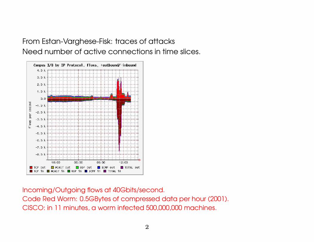
From Estan-Varghese-Fisk: traces of attacksNeed number of active connections in time slices.

Incoming/Outgoing flows at 40Gbits/second.Code Red Worm: 0.5GBytes of compressed data per hour (2001).CISCO: in 11 minutes, a worm infected 500,000,000 machines.

2

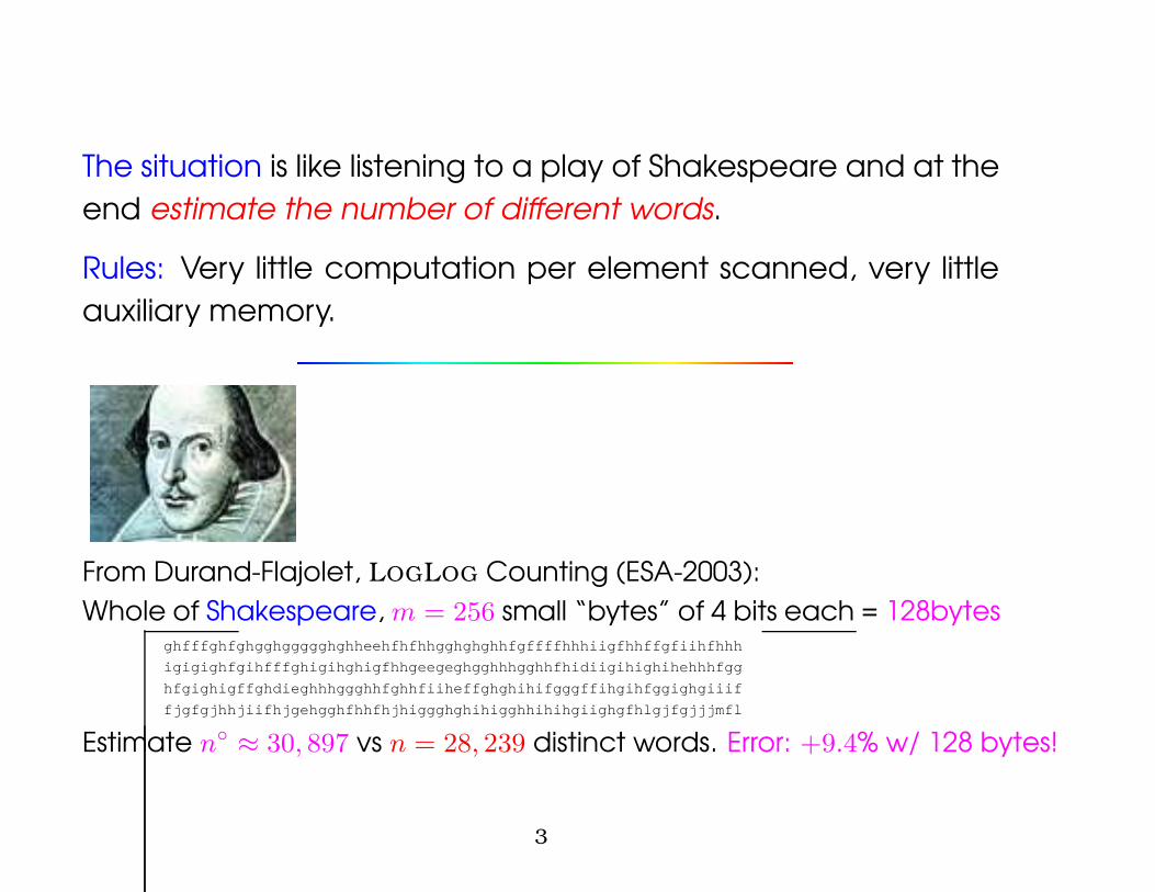
The situation is like listening to a play of Shakespeare and at theend estimate the number of different words.

Rules: Very little computation per element scanned, very littleauxiliary memory.

From Durand-Flajolet, LOGLOG Counting (ESA-2003):Whole of Shakespeare, m = 256 small “bytes” of 4 bits each = 128bytes

ghfffghfghgghggggghghheehfhfhhgghghghhfgffffhhhiigfhhffgfiihfhhh

igigighfgihfffghigihghigfhhgeegeghgghhhgghhfhidiigihighihehhhfgg

hfgighigffghdieghhhggghhfghhfiiheffghghihifgggffihgihfggighgiiif

fjgfgjhhjiifhjgehgghfhhfhjhiggghghihigghhihihgiighgfhlgjfgjjjmfl

Estimate n◦ ≈ 30, 897 vs n = 28, 239 distinct words. Error: +9.4% w/ 128 bytes!

3

Uses:— Routers: intrusion, flow monitoring & control

— Databases: Query optimization, cf M ∪ M′ for multisets; Esti-

mating the size of queries & “sketches”.

— Statistics gathering: on the fly, fast and with little memoryeven on “unclean” data ' layer 0 of “data mining”.

4

This talk:

• Estimating characteristics of large data streams— sampling; size & cardinality & nonuniformity index [F1, F0, F2]; power of randomization via hashing

� Gains by a factor of >400 [Palmer et al.]

• Analysis of algorithms— generating functions, complex asymptotics, Mellin transforms

� Nice problems for theoreticians.

• Theory and Practice— Interplay of analysis and design ; super-optimized algorithms.

5

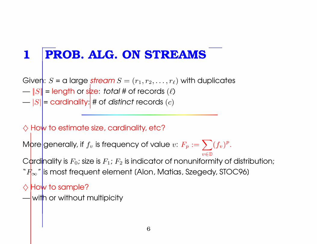
1 PROB. ALG. ON STREAMS

Given: S = a large stream S = (r1, r2, . . . , r`) with duplicates— ||S|| = length or size: total # of records (`)— |S| = cardinality: # of distinct records (c)

♦ How to estimate size, cardinality, etc?

More generally, if fv is frequency of value v: Fp :=X

v∈D

(fv)p.

Cardinality is F0; size is F1; F2 is indicator of nonuniformity of distribution;“F∞” is most frequent element [Alon, Matias, Szegedy, STOC96]

♦ How to sample?— with or without multipicity

6

The

Angel

——

Daemon

Model

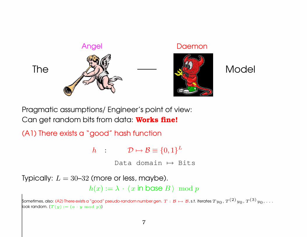
Pragmatic assumptions/ Engineer’s point of view:Can get random bits from data: Works fine!

(A1) There exists a “good” hash function

h : D 7→ B ≡ {0, 1}L

Data domain 7→ Bits

Typically: L = 30–32 (more or less, maybe).h(x) := λ · 〈x in base B 〉 mod p

Sometimes, also: (A2) There exists a “good” pseudo-random number gen. T : B 7→ B, s.t. iterates Ty0, T (2)y0, T (3)y0, . . .

look random. [T (y) := (a · y mod p)]

7

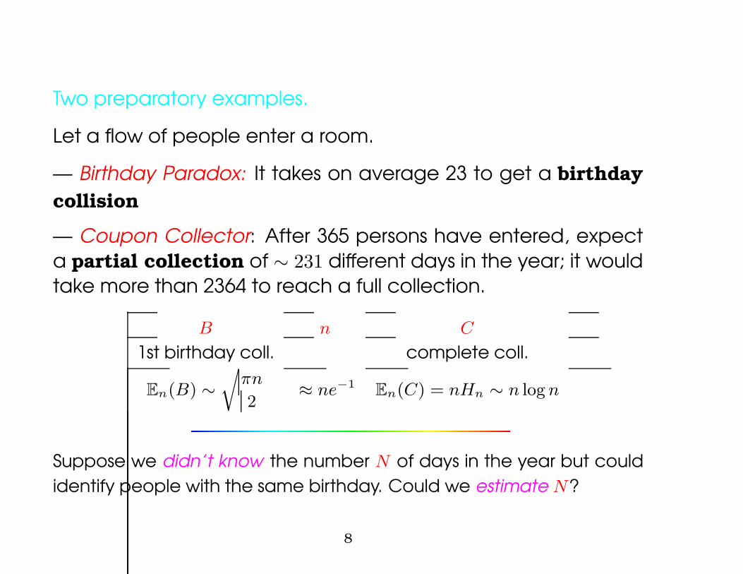
Two preparatory examples.

Let a flow of people enter a room.

— Birthday Paradox: It takes on average 23 to get a birthdaycollision

— Coupon Collector: After 365 persons have entered, expecta partial collection of ∼ 231 different days in the year; it wouldtake more than 2364 to reach a full collection.

B n C

1st birthday coll. complete coll.

En(B) ∼r

πn

2≈ ne−1

En(C) = nHn ∼ n log n

Suppose we didn’t know the number N of days in the year but couldidentify people with the same birthday. Could we estimate N?

8

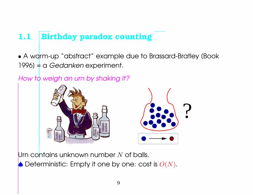
1.1 Birthday paradox counting

• A warm-up “abstract” example due to Brassard-Bratley [Book1996] = a Gedanken experiment.

How to weigh an urn by shaking it?

?

Urn contains unknown number N of balls.♠ Deterministic: Empty it one by one: cost is O(N).

9

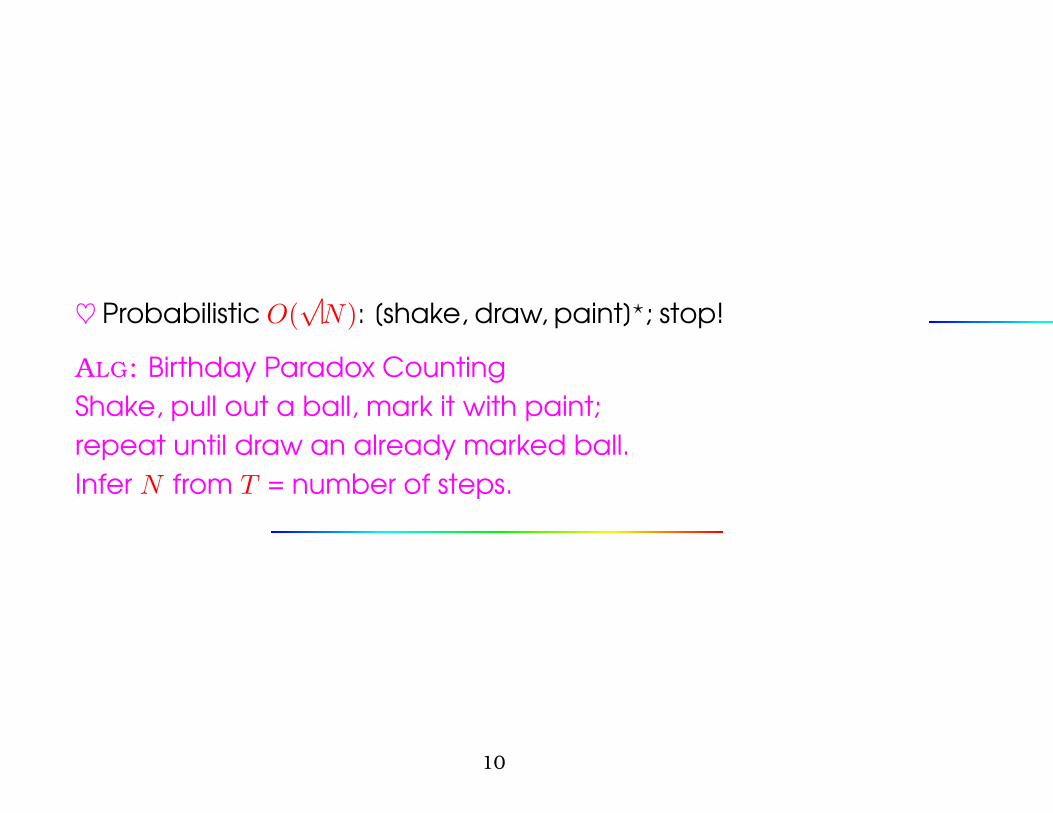
♥ Probabilistic O(√

N): [shake, draw, paint]?; stop!

ALG: Birthday Paradox CountingShake, pull out a ball, mark it with paint;repeat until draw an already marked ball.Infer N from T = number of steps.

10

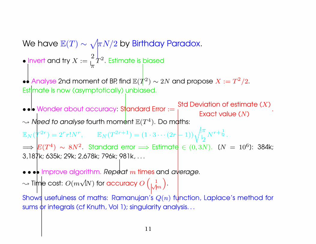
We have E(T ) ∼√

πN/2 by Birthday Paradox.

• Invert and try X :=2

πT 2. Estimate is biased

•• Analyse 2nd moment of BP, find E(T 2) ∼ 2N and propose X := T 2/2.Estimate is now (asymptotically) unbiased.

• • • Wonder about accuracy: Standard Error :=Std Deviation of estimate (X)

Exact value (N).

; Need to analyse fourth moment E(T 4). Do maths:

EN (T 2r) = 2rr!Nr, EN (T 2r+1) = (1 · 3 · · · (2r − 1))

rπ

2Nr+ 1

2 .

=⇒ E(T 4) ∼ 8N2. Standard error =⇒ Estimate ∈ (0, 3N). [N = 106]: 384k;3,187k; 635k; 29k; 2,678k; 796k; 981k, . . .

• • •• Improve algorithm. Repeat m times and average.

; Time cost: O(m√

N) for accuracy O“

1√m

”

.

Shows usefulness of maths: Ramanujan’s Q(n) function, Laplace’s method forsums or integrals (cf Knuth, Vol 1); singularity analysis. . .

11

1.2 Coupon Collector Counting

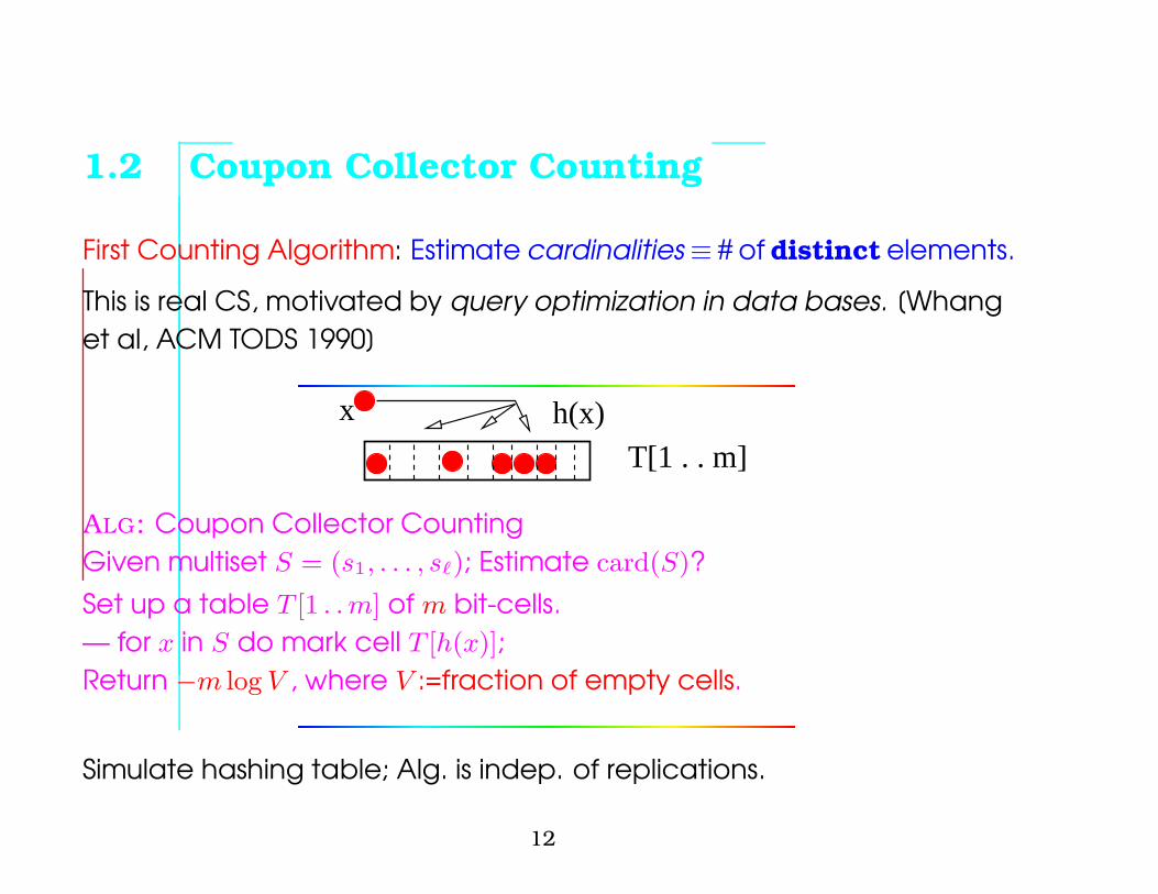
First Counting Algorithm: Estimate cardinalities≡ # of distinct elements.

This is real CS, motivated by query optimization in data bases. [Whanget al, ACM TODS 1990]

x h(x)

T[1 . . m]

ALG: Coupon Collector CountingGiven multiset S = (s1, . . . , s`); Estimate card(S)?Set up a table T [1 . . m] of m bit-cells.— for x in S do mark cell T [h(x)];Return −m log V , where V :=fraction of empty cells.

Simulate hashing table; Alg. is indep. of replications.

12

Let n be sought cardinality. Then α := n/m is filling ratio. Expect V ≈ e−α

empty cells by classical analysis of occupancy. Distribution is concen-trated. Invert!

Count cardinalities till Nmax using 110

Nmax bits, for accuracy (standarderror) = 2%.

Generating functions for occupancy; Stirling numbers; basic depois-sonization.

13

2 SAMPLING

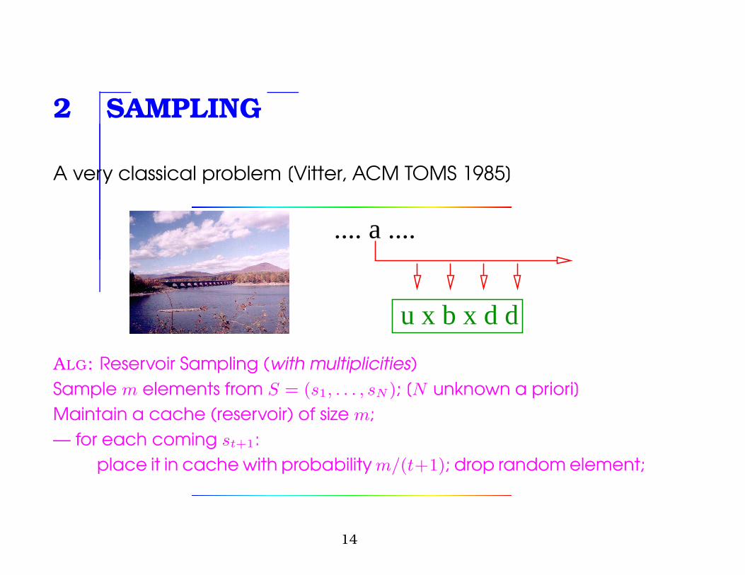
A very classical problem [Vitter, ACM TOMS 1985]

u x b x d d

.... a ....

ALG: Reservoir Sampling (with multiplicities)Sample m elements from S = (s1, . . . , sN ); [N unknown a priori]Maintain a cache (reservoir) of size m;— for each coming st+1:

place it in cache with probability m/(t+1); drop random element;

14

Math: Need analysis of skipping probabilities.Complexity of Vitter’s best alg. is O(m log N).

Useful for building “sketches”, order-preserving H-fns & DS.

15

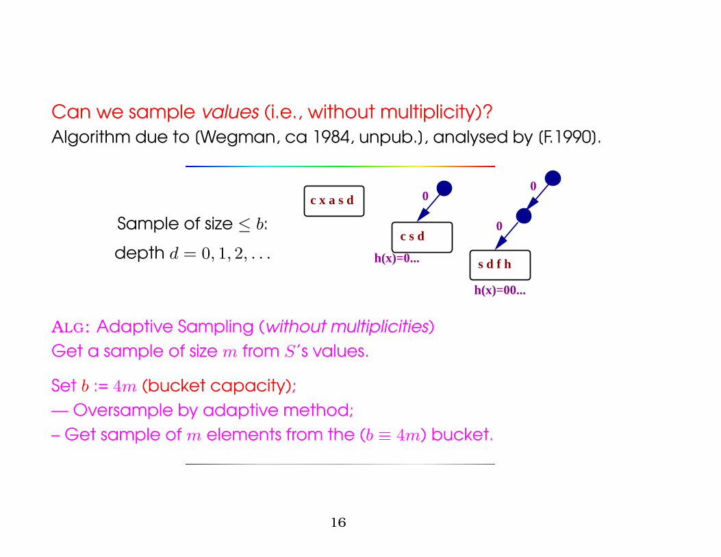
Can we sample values (i.e., without multiplicity)?Algorithm due to [Wegman, ca 1984, unpub.], analysed by [F.1990].

Sample of size ≤ b:

depth d = 0, 1, 2, . . .

h(x)=00...

0

0

s d f h

0

c s d

h(x)=0...

c x a s d

ALG: Adaptive Sampling (without multiplicities)Get a sample of size m from S’s values.

Set b := 4m (bucket capacity);— Oversample by adaptive method;– Get sample of m elements from the (b ≡ 4m) bucket.

16

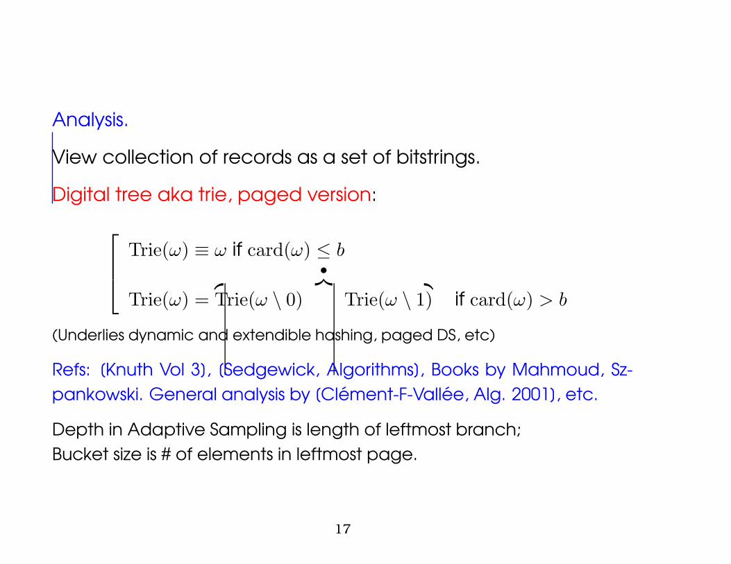
Analysis.

View collection of records as a set of bitstrings.

Digital tree aka trie, paged version:

Trie(ω) ≡ ω if card(ω) ≤ b

Trie(ω) =

•︷ ︸︸ ︷

Trie(ω \ 0) Trie(ω \ 1) if card(ω) > b

(Underlies dynamic and extendible hashing, paged DS, etc)

Refs: [Knuth Vol 3], [Sedgewick, Algorithms], Books by Mahmoud, Sz-pankowski. General analysis by [Clement-F-Vallee, Alg. 2001], etc.

Depth in Adaptive Sampling is length of leftmost branch;Bucket size is # of elements in leftmost page.

17

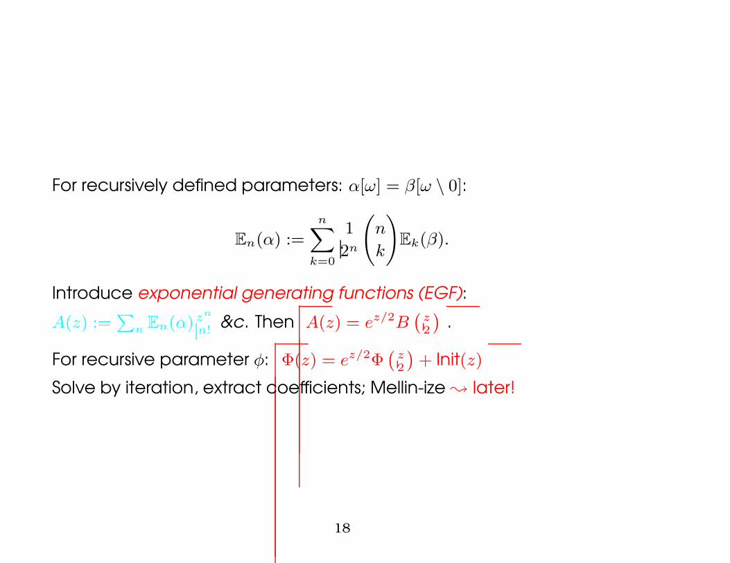
For recursively defined parameters: α[ω] = β[ω \ 0]:

En(α) :=

nX

k=0

1

2n

n

k

!Ek(β).

Introduce exponential generating functions (EGF):

A(z) :=P

n En(α) zn

n!&c. Then A(z) = ez/2B

`z2

´.

For recursive parameter φ: Φ(z) = ez/2Φ`

z2

´+ Init(z)

Solve by iteration, extract coefficients; Mellin-ize ; later!

18

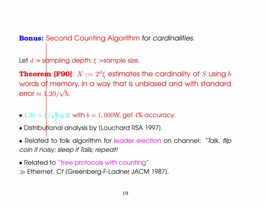
Bonus: Second Counting Algorithm for cardinalities.

Let d := sampling depth; ξ :=sample size.

Theorem [F90]: X := 2dξ estimates the cardinality of S using b

words of memory, in a way that is unbiased and with standarderror ≈ 1.20/

√b.

• 1.20.= 1/

√log 2: with b = 1, 000W, get 4% accuracy.

• Distributional analysis by [Louchard RSA 1997].

• Related to folk algorithm for leader election on channel: “Talk, flipcoin if noisy; sleep if Tails; repeat!

• Related to “tree protocols with counting”� Ethernet. Cf [Greenberg-F-Ladner JACM 1987].

19

3 APPROXIMATE COUNTING

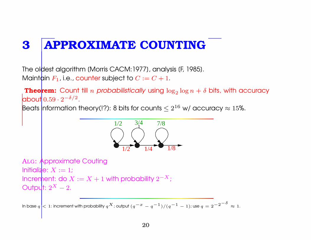
The oldest algorithm [Morris CACM:1977], analysis [F, 1985].Maintain F1, i.e., counter subject to C := C + 1.

Theorem: Count till n probabilistically using log2 log n + δ bits, with accuracyabout 0.59 · 2−δ/2.Beats information theory(!?): 8 bits for counts ≤ 216 w/ accuracy ≈ 15%.

1

1/2 1/4

1/2 3/4 7/8

1/8

ALG: Approximate CoutingInitialize: X := 1;Increment: do X := X + 1 with probability 2−X ;Output: 2X − 2.

In base q < 1: increment with probability qX ; output (q−x− q−1)/(q−1

− 1); use q = 2−2−δ≈ 1.

20

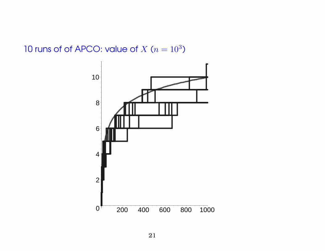
10 runs of of APCO: value of X (n = 103)

0

2

4

6

8

10

200 400 600 800 1000

21

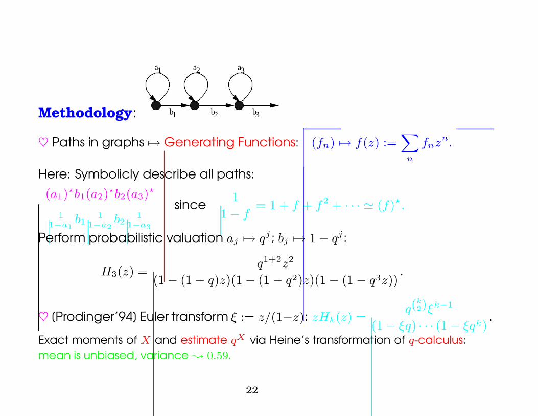
Methodology: b b b1 2 3

a1 a2 a3

♥ Paths in graphs 7→ Generating Functions: (fn) 7→ f(z) :=X

n

fnzn.

Here: Symbolicly describe all paths:(a1)

?b1(a2)?b2(a3)

?

11−a1

b11

1−a2b2

11−a3

since1

1− f= 1 + f + f2 + · · · ' (f)?.

Perform probabilistic valuation aj 7→ qj ; bj 7→ 1− qj :

H3(z) =q1+2z2

(1− (1− q)z)(1− (1− q2)z)(1− (1− q3z)).

♥ [Prodinger’94] Euler transform ξ := z/(1−z): zHk(z) =q(

k2)ξk−1

(1− ξq) · · · (1− ξqk).

Exact moments of X and estimate qX via Heine’s transformation of q-calculus:mean is unbiased, variance ; 0.59.

22

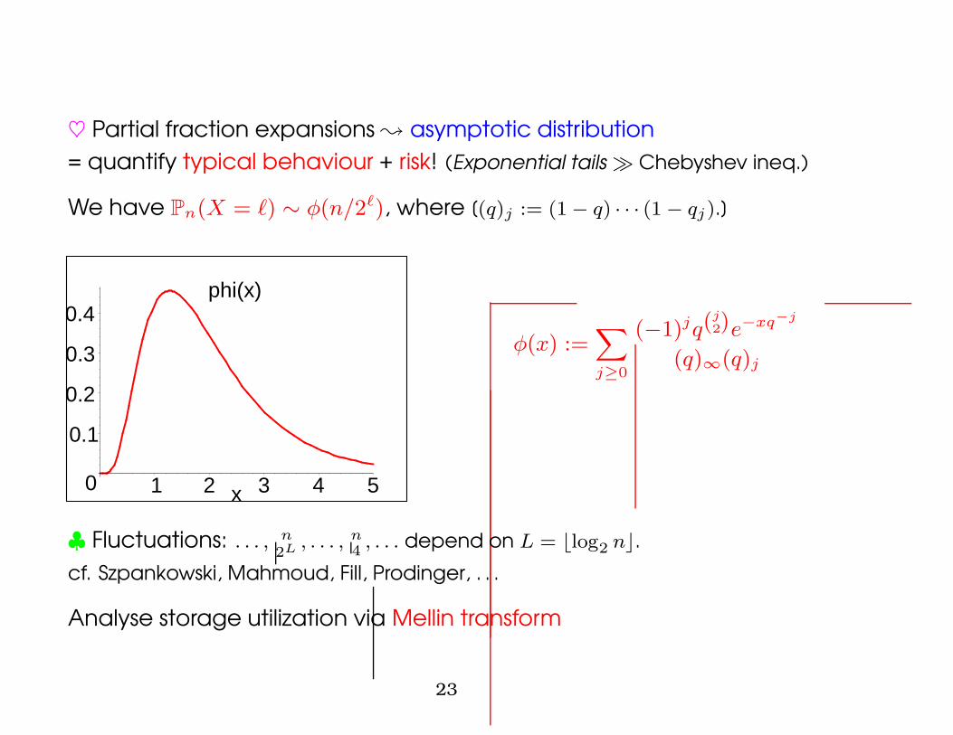
♥ Partial fraction expansions ; asymptotic distribution= quantify typical behaviour + risk! (Exponential tails � Chebyshev ineq.)

We have Pn(X = `) ∼ φ(n/2`), where [(q)j := (1 − q) · · · (1 − qj).]

phi(x)

0

0.1

0.2

0.3

0.4

1 2 3 4 5x

φ(x) :=X

j≥0

(−1)jq(j2)e−xq−j

(q)∞(q)j

♣ Fluctuations: . . . , n2L , . . . , n

4, . . . depend on L = blog2 nc.

cf. Szpankowski, Mahmoud, Fill, Prodinger, . . .

Analyse storage utilization via Mellin transform

23

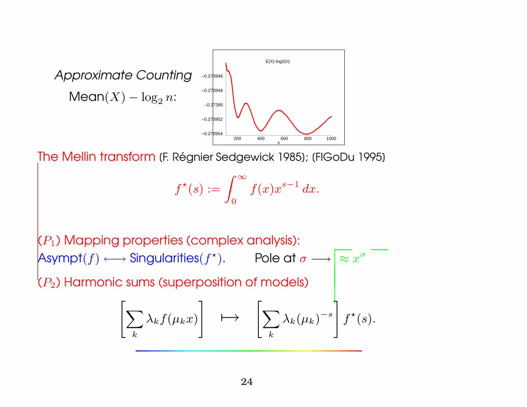
Approximate Counting

Mean(X)− log2 n:

E(X)-log2(n)

–0.273954

–0.273952

–0.27395

–0.273948

–0.273946

200 400 600 800 1000x

The Mellin transform [F. Regnier Sedgewick 1985]; [FlGoDu 1995]

f?(s) :=

Z ∞

0

f(x)xs−1 dx.

(P1) Mapping properties (complex analysis):Asympt(f)←→ Singularities(f?). Pole at σ −→ ≈ xσ

(P2) Harmonic sums (superposition of models)"X

k

λkf(µkx)

#7→

"X

k

λk(µk)−s

#f?(s).

24

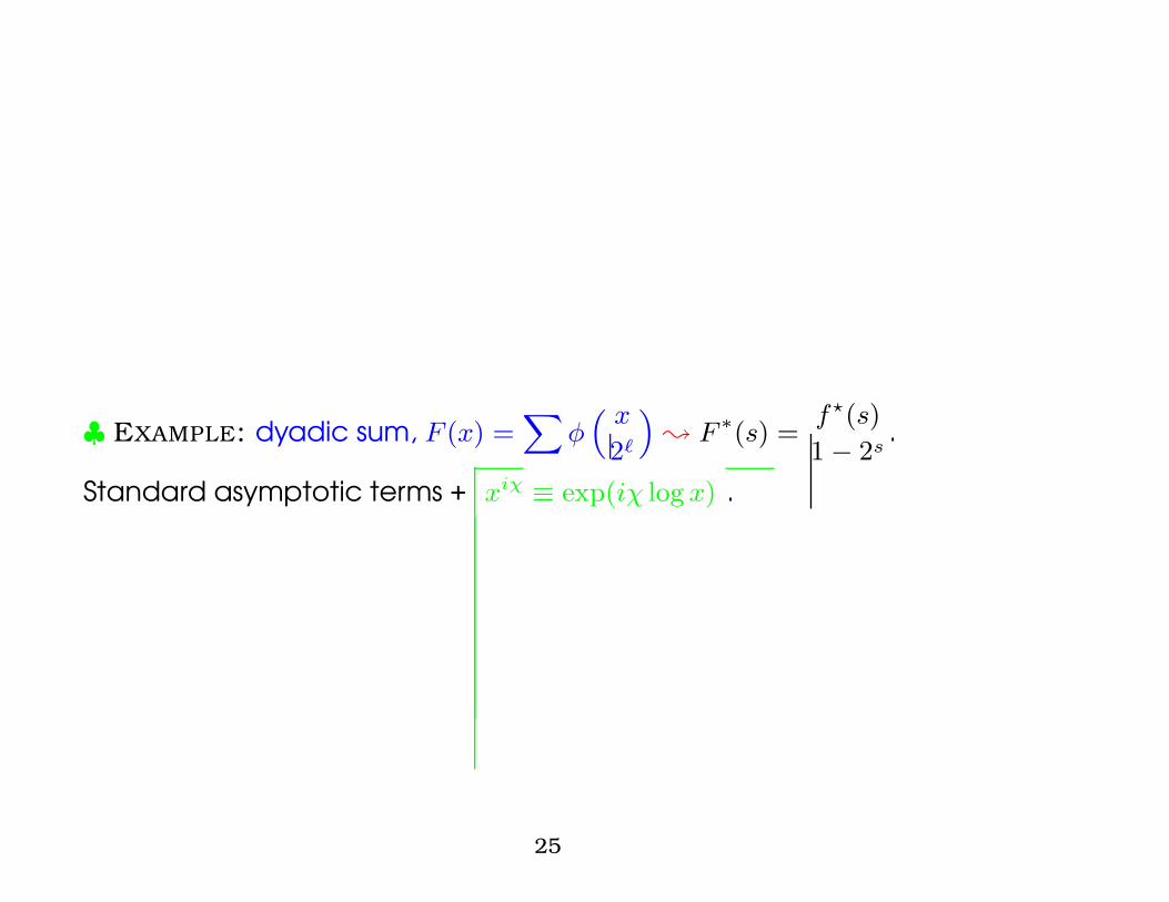
♣ EXAMPLE: dyadic sum, F (x) =X

φ“ x

2`

”; F ∗(s) =

f?(s)

1− 2s.

Standard asymptotic terms + xiχ ≡ exp(iχ log x) .

25

Cultural flashes

— Morris [1977]: Couting a large number of events in small memory.— The power of probabilistic machines & approximation [Freivalds IFIP1977]— The FTP protocol: Additive Increase Multiplicative Decrease (AIMD)leads to similar functions [Robert et al, 2001]— Probability theory: Exponentials of Poisson processes [Yor et al, 2001]

26

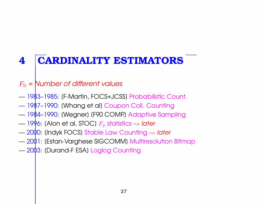
4 CARDINALITY ESTIMATORS

F0 = Number of different values

— 1983–1985: [F-Martin, FOCS+JCSS] Probabilistic Count.— 1987–1990: [Whang et al] Coupon Coll. Counting— 1984–1990: [Wegner] [F90 COMP.] Adaptive Sampling— 1996: [Alon et al, STOC] Fp statistics ; later— 2000: [Indyk FOCS] Stable Law Counting ; later— 2001: [Estan-Varghese SIGCOMM] Multiresolution Bitmap— 2003: [Durand-F ESA] Loglog Counting

27

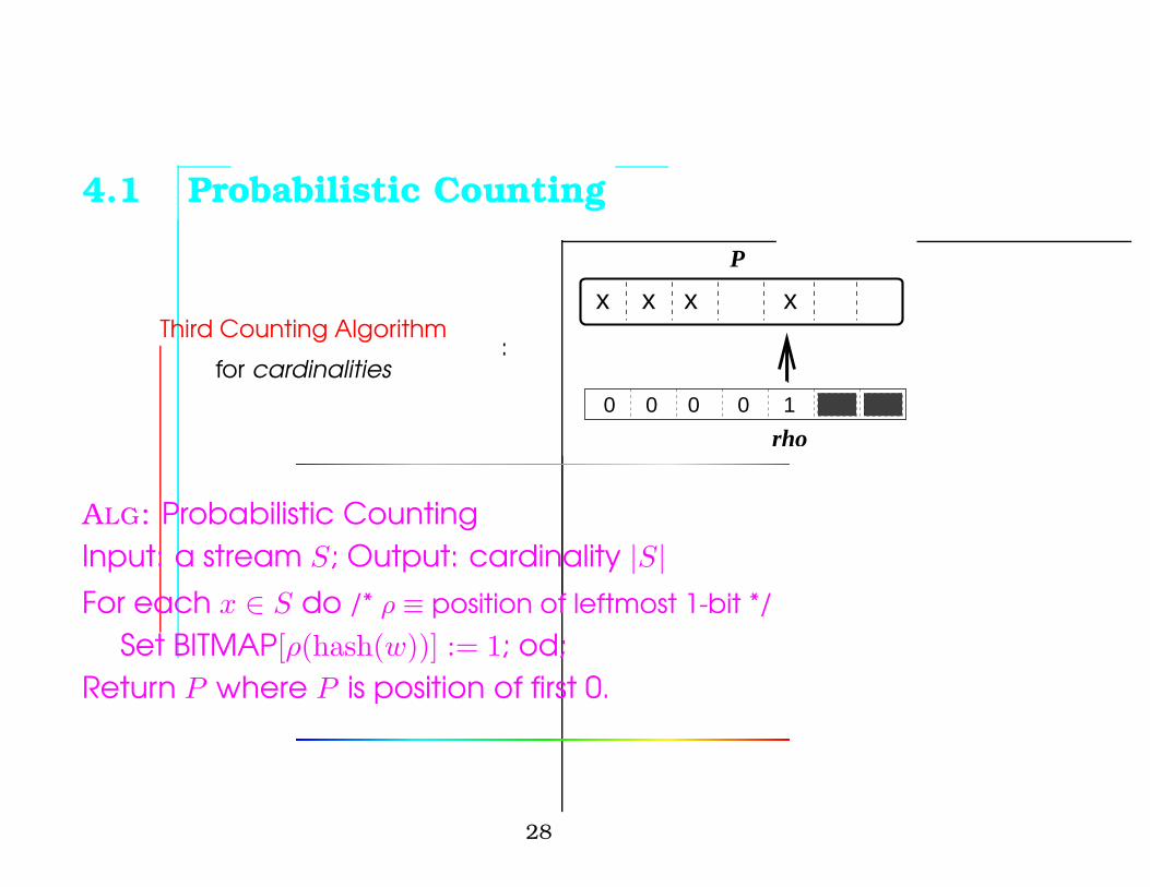
4.1 Probabilistic Counting

Third Counting Algorithm

for cardinalities:

x x x x

0 0 0 0 1

P

rho

ALG: Probabilistic CountingInput: a stream S; Output: cardinality |S|For each x ∈ S do /* ρ ≡ position of leftmost 1-bit */

Set BITMAP[ρ(hash(w))] := 1; od;Return P where P is position of first 0.

28

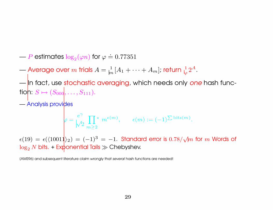
— P estimates log2(ϕn) for ϕ.= 0.77351

— Average over m trials A = 1m

[A1 + · · ·+ Am]; return 1ϕ2A.

— In fact, use stochastic averaging, which needs only one hash func-tion: S 7→ (S000, . . . , S111).

— Analysis provides

ϕ =eγ

√2

Y

m≥2

? mε(m), ε(m) := (−1)P

bits(m).

ε(19) = ε(〈10011〉2) = (−1)3 = −1. Standard error is 0.78/√

m for m Words oflog2 N bits. + Exponential Tails � Chebyshev.

[AMS96] and subsequent literature claim wrongly that several hash functions are needed!

29

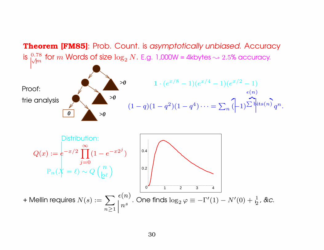
Theorem [FM85]: Prob. Count. is asymptotically unbiased. Accuracyis 0.78√

mfor m Words of size log2 N . E.g. 1,000W = 4kbytes ; 2.5% accuracy.

Proof:

trie analysis

>0

>0

>00

1 · (ex/8 − 1)(ex/4 − 1)(ex/2 − 1)

(1 − q)(1 − q2)(1 − q4) · · · =P

n

ε(n)z }| {

(−1)P

bits(n) qn.

Distribution:

Q(x) := e−x/2∞Y

j=0

(1 − e−x2j)

Pn(X = `) ∼ Q“ n

2`

”

0

0.2

0.4

1 2 3 4

+ Mellin requires N(s) :=X

n≥1

ε(n)

ns. One finds log2 ϕ ≡ −Γ′(1) − N ′(0) + 1

2, &c.

30

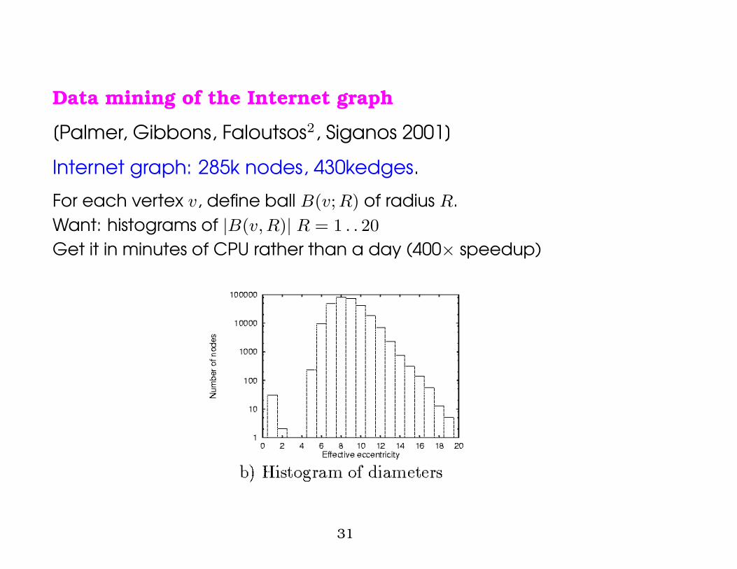
Data mining of the Internet graph

[Palmer, Gibbons, Faloutsos2, Siganos 2001]

Internet graph: 285k nodes, 430kedges.

For each vertex v, define ball B(v;R) of radius R.Want: histograms of |B(v, R)| R = 1 . . 20

Get it in minutes of CPU rather than a day (400× speedup)

31

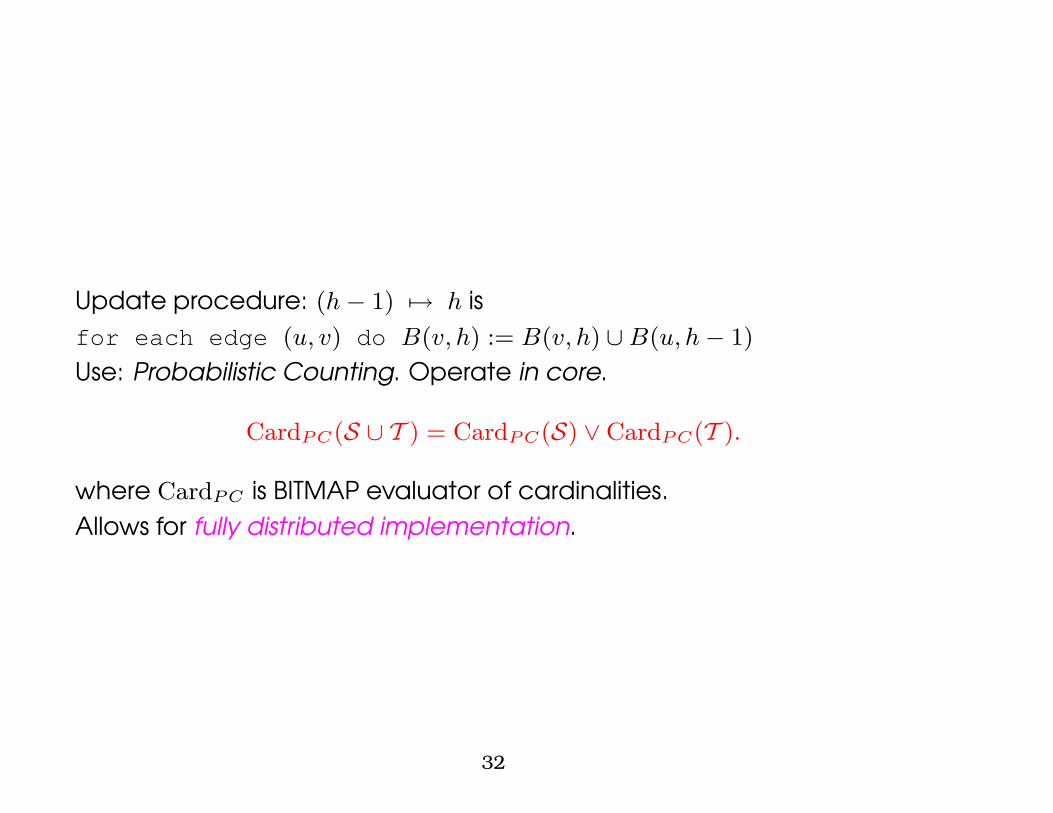
Update procedure: (h− 1) 7→ h isfor each edge (u, v) do B(v, h) := B(v, h) ∪B(u, h− 1)

Use: Probabilistic Counting. Operate in core.

CardPC(S ∪ T ) = CardPC(S) ∨ CardPC(T ).

where CardPC is BITMAP evaluator of cardinalities.Allows for fully distributed implementation.

32

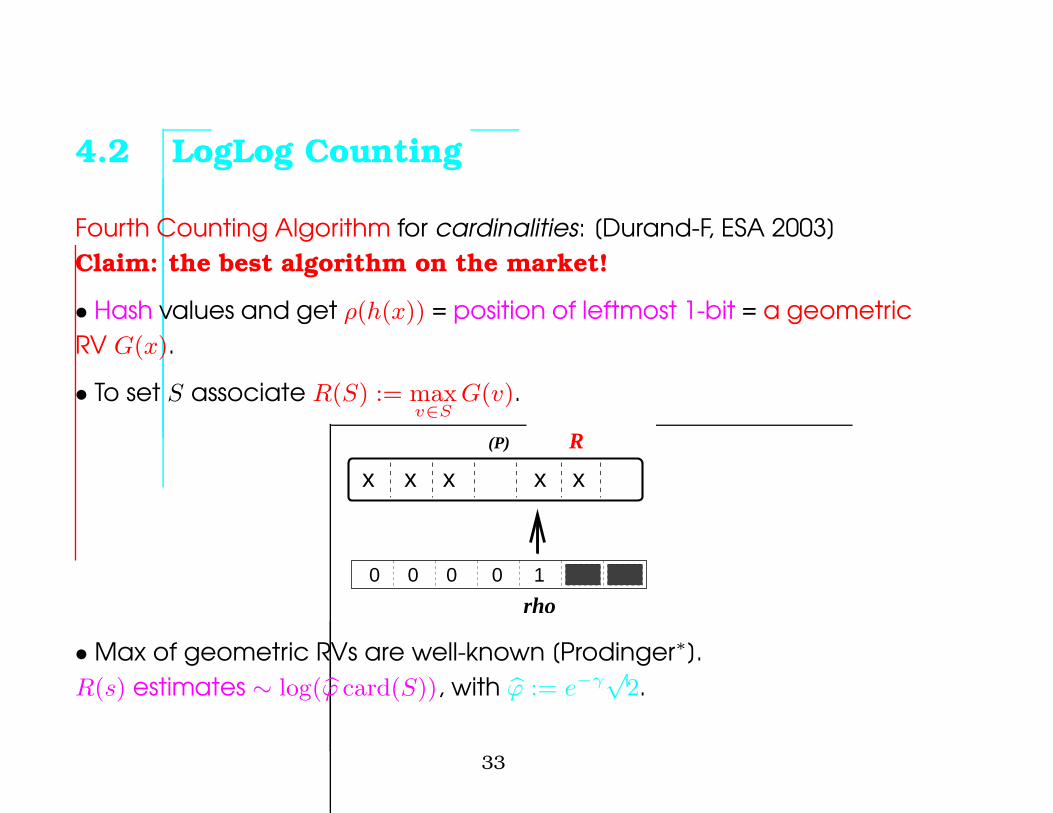
4.2 LogLog Counting

Fourth Counting Algorithm for cardinalities: [Durand-F, ESA 2003]Claim: the best algorithm on the market!

• Hash values and get ρ(h(x)) = position of leftmost 1-bit = a geometricRV G(x).

• To set S associate R(S) := maxv∈S

G(v).

x x x x

0 0 0 0 1

rho

x

R(P)

•Max of geometric RVs are well-known [Prodinger∗].R(s) estimates ∼ log(bϕ card(S)), with bϕ := e−γ

√2.

33

• Do stochastic averaging with m = 2`:E.g., S ∼= 〈S00, S01, S10, S11〉: count separately.

Returnm

bϕ 2Average .

++ Switch to Coupon Collector Counting for small cardinalities.++ Optimize by pruning discrepant values ; superLogLog.

34

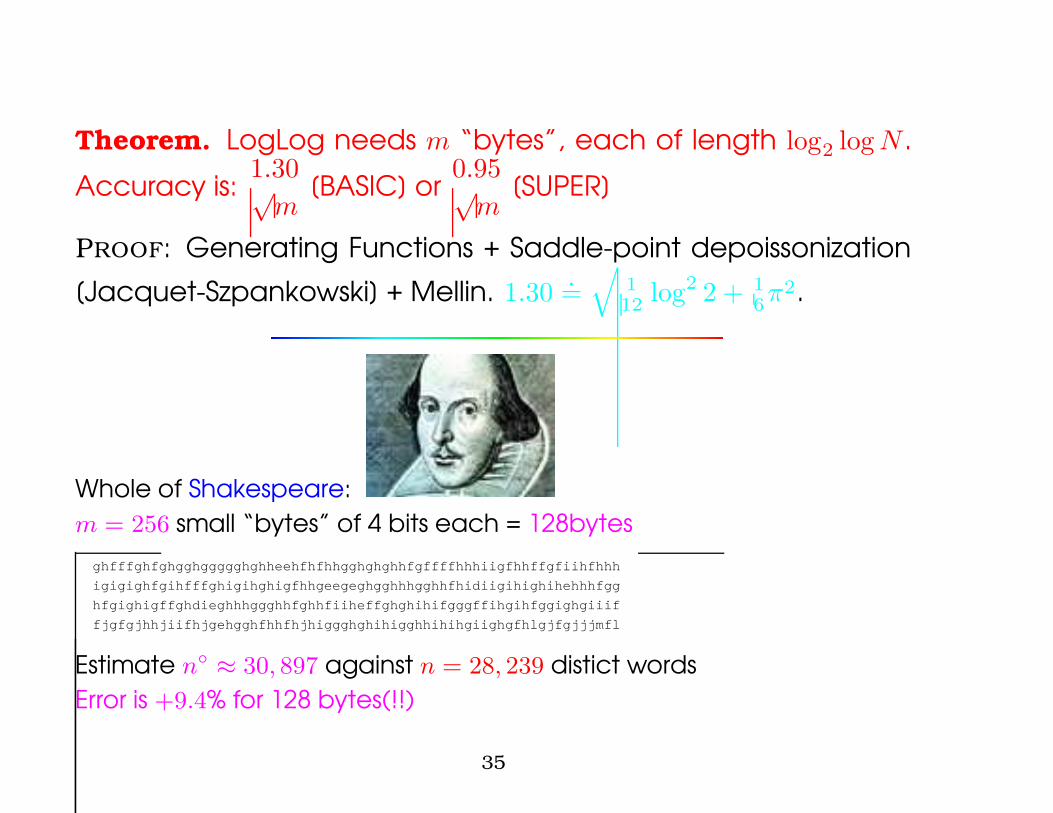
Theorem. LogLog needs m “bytes”, each of length log2log N .

Accuracy is:1.30√

m[BASIC] or

0.95√m

[SUPER]

PROOF: Generating Functions + Saddle-point depoissonization

[Jacquet-Szpankowski] + Mellin. 1.30.=

√1

12log2 2 + 1

6π2.

Whole of Shakespeare:m = 256 small “bytes” of 4 bits each = 128bytes

ghfffghfghgghggggghghheehfhfhhgghghghhfgffffhhhiigfhhffgfiihfhhh

igigighfgihfffghigihghigfhhgeegeghgghhhgghhfhidiigihighihehhhfgg

hfgighigffghdieghhhggghhfghhfiiheffghghihifgggffihgihfggighgiiif

fjgfgjhhjiifhjgehgghfhhfhjhiggghghihigghhihihgiighgfhlgjfgjjjmfl

Estimate n◦ ≈ 30, 897 against n = 28, 239 distict wordsError is +9.4% for 128 bytes(!!)

35

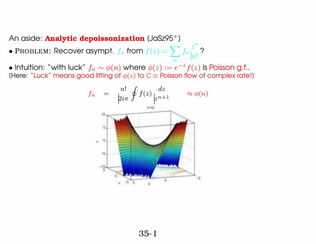
An aside: Analytic depoissonization [JaSz95+]

• PROBLEM: Recover asympt. fn from f(z) =X

n

fnzn

n!?

• Intuition: “with luck” fn ∼ φ(n) where φ(z) := e−zf(z) is Poisson g.f..[Here: “Luck” means good lifting of φ(z) to C ≡ Poisson flow of complex rate!]

fn =n!

2iπ

I

f(z)dz

zn+1≈ φ(n)

35-1

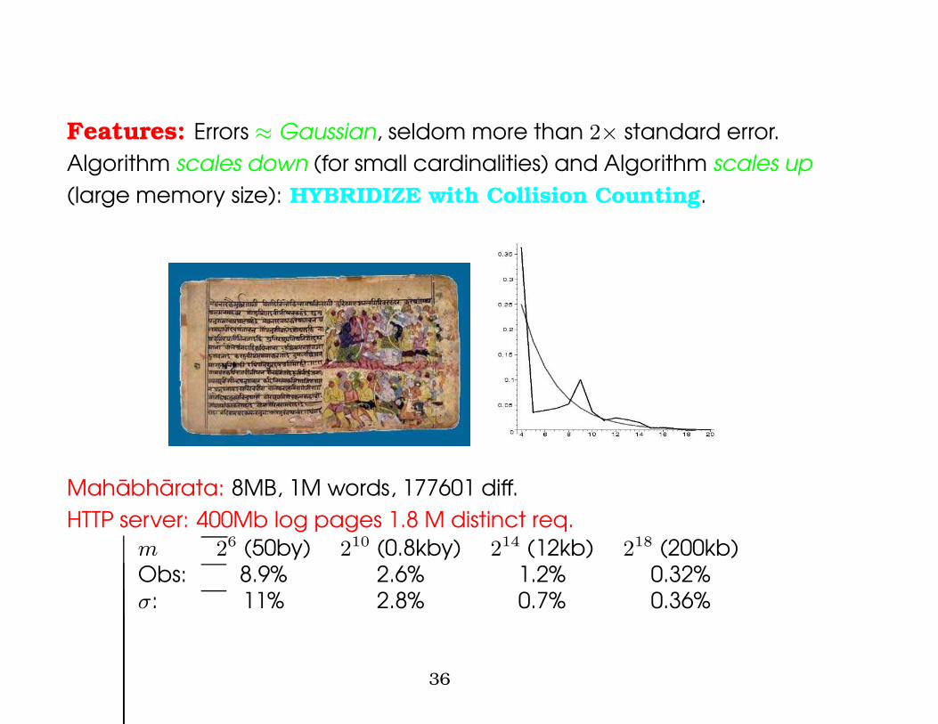
Features: Errors ≈ Gaussian, seldom more than 2× standard error.Algorithm scales down (for small cardinalities) and Algorithm scales up(large memory size): HYBRIDIZE with Collision Counting.

Mahabharata: 8MB, 1M words, 177601 diff.HTTP server: 400Mb log pages 1.8 M distinct req.

m 26 (50by) 210 (0.8kby) 214 (12kb) 218 (200kb)Obs: 8.9% 2.6% 1.2% 0.32%σ: 11% 2.8% 0.7% 0.36%

36

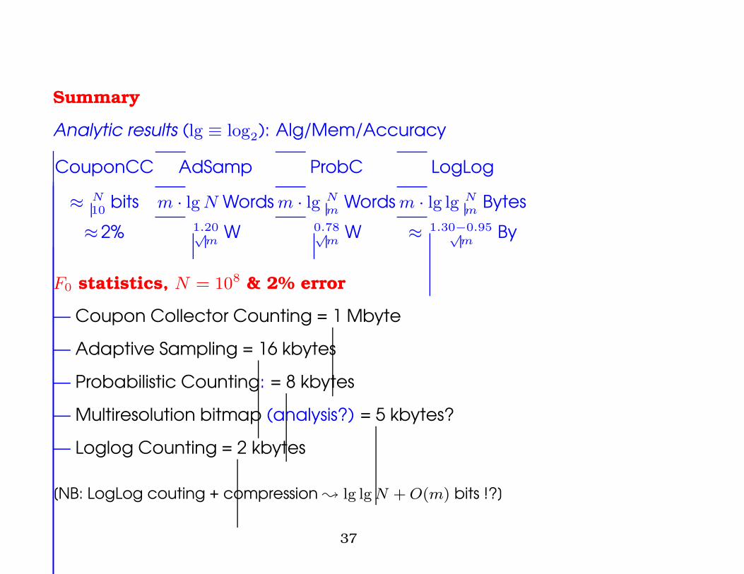
Summary

Analytic results (lg ≡ log2): Alg/Mem/Accuracy

CouponCC AdSamp ProbC LogLog

≈ N10

bits m · lg N Words m · lg Nm

Words m · lg lg Nm

Bytes

≈ 2% 1.20√m

W 0.78√m

W ≈ 1.30−0.95√m

By

F0 statistics, N = 108 & 2% error

— Coupon Collector Counting = 1 Mbyte

— Adaptive Sampling = 16 kbytes

— Probabilistic Counting: = 8 kbytes

— Multiresolution bitmap (analysis?) = 5 kbytes?

— Loglog Counting = 2 kbytes

[NB: LogLog couting + compression ; lg lg N + O(m) bits !?]

37

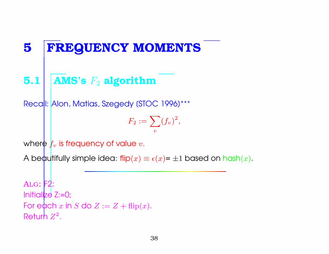
5 FREQUENCY MOMENTS

5.1 AMS’s F2 algorithm

Recall: Alon, Matias, Szegedy [STOC 1996]???

F2 :=X

v

(fv)2,

where fv is frequency of value v.

A beautifully simple idea: flip(x) ≡ ε(x)= ±1 based on hash(x).

ALG: F2;Initialize Z:=0;For each x in S do Z := Z + flip(x).Return Z2.

38

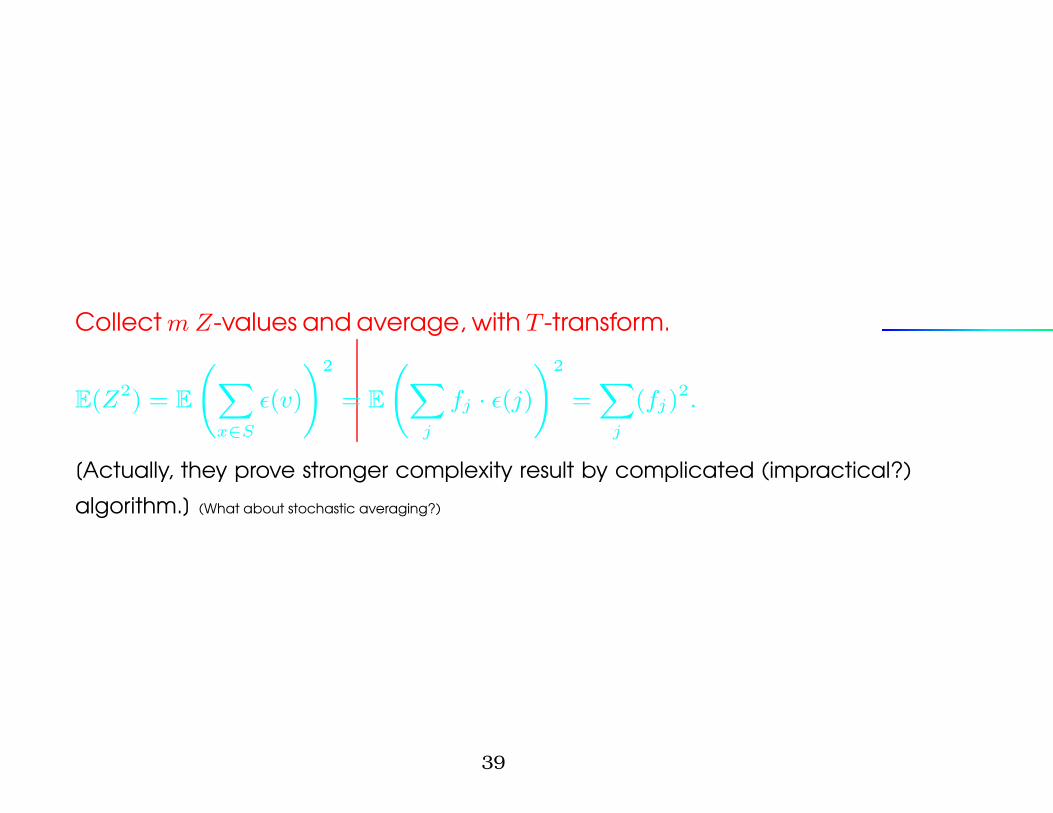
Collect m Z-values and average, with T -transform.

E(Z2) = E

X

x∈S

ε(v)

!2

= E

X

j

fj · ε(j)!2

=X

j

(fj)2.

[Actually, they prove stronger complexity result by complicated (impractical?)

algorithm.] (What about stochastic averaging?)

39

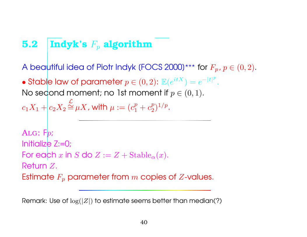
5.2 Indyk’s Fp algorithm

A beautiful idea of Piotr Indyk [FOCS 2000]??? for Fp, p ∈ (0, 2).

• Stable law of parameter p ∈ (0, 2): E(eitX) = e−|t|p .

No second moment; no 1st moment if p ∈ (0, 1).

c1X1 + c2X2

L∼= µX, with µ := (cp1

+ cp2)1/p.

ALG: Fp;Initialize Z:=0;For each x in S do Z := Z + Stableα(x).Return Z.Estimate Fp parameter from m copies of Z-values.

Remark: Use of log(|Z|) to estimate seems better than median(?)

40

6 CONCLUSIONS

For streams, using practically O(1) storage, one can:— Sample positions and even distinct values;— Estimate F0, F1, F2, Fp (0 < p ≤ 2) even for huge data sets;— Need no assumption on nature of data.

♥♥♥♥♥♥

The algorithms are based on randomization 7→ Analysis fully applies— They work exactly as predicted on real-life data;— They often have a wonderfully elegant structure;— Their analysis involves beautiful methods for AofA: “Symbolic modelling

by generating functions, Singularity analysis, Saddle Point and analytic depois-

sonization, Mellin transforms, stable laws and Mittag-Leffler functions, etc.”

41

That’s All, Folks!

42