Bobcat Abundance and Habitat Selection on the Utah Test

Brigham Young University Brigham Young University

BYU ScholarsArchive BYU ScholarsArchive

Theses and Dissertations

2018-12-01

Bobcat Abundance and Habitat Selection on the Utah Test and Bobcat Abundance and Habitat Selection on the Utah Test and

Training Range Training Range

Kyle David Muncey Brigham Young University

Follow this and additional works at: https://scholarsarchive.byu.edu/etd

Part of the Life Sciences Commons

BYU ScholarsArchive Citation BYU ScholarsArchive Citation Muncey, Kyle David, "Bobcat Abundance and Habitat Selection on the Utah Test and Training Range" (2018). Theses and Dissertations. 7710. https://scholarsarchive.byu.edu/etd/7710

This Thesis is brought to you for free and open access by BYU ScholarsArchive. It has been accepted for inclusion in Theses and Dissertations by an authorized administrator of BYU ScholarsArchive. For more information, please contact [email protected], [email protected].

http://home.byu.edu/home/

http://home.byu.edu/home/

https://scholarsarchive.byu.edu/

https://scholarsarchive.byu.edu/etd

https://scholarsarchive.byu.edu/etd?utm_source=scholarsarchive.byu.edu%2Fetd%2F7710&utm_medium=PDF&utm_campaign=PDFCoverPages

http://network.bepress.com/hgg/discipline/1016?utm_source=scholarsarchive.byu.edu%2Fetd%2F7710&utm_medium=PDF&utm_campaign=PDFCoverPages

https://scholarsarchive.byu.edu/etd/7710?utm_source=scholarsarchive.byu.edu%2Fetd%2F7710&utm_medium=PDF&utm_campaign=PDFCoverPages

mailto:[email protected],%[email protected]

Bobcat Abundance and Habitat Selection on the Utah Test and Training Range

Kyle David Muncey

A thesis submitted to the faculty of Brigham Young University

in partial fulfillment of the requirements for the degree of

Master of Science

Tom S. Smith, Chair Steven L. Petersen Randy T. Larsen

Department of Plant and Wildlife Sciences

Brigham Young University

Copyright ©2018 Kyle David Muncey

All Rights Reserved

ABSTRACT

Bobcat Abundance and Habitat Selection on the Utah Test and Training Range

Kyle David Muncey Department of Plant and Wildlife Sciences, BYU

Master of Science

Remote cameras have become a popular tool for monitoring wildlife. We used remote cameras to estimate bobcat (Lynx rufus) population abundance on the Utah Test and Training Range during two sample periods between 2015 and 2017. We used two statistical methods, closed capture mark-recapture (CMR) and mark-resight Poisson log-normal (PNE), to estimate bobcat abundance within the study area. We used the maximum mean distance moved method (MMDM) to calculate the effective sample area for estimating density. Additionally, we captured bobcats and estimated home range using minimum convex polygon (MCP) and kernel density estimation (KDE) methods. Bobcat abundance on the UTTR was 35-48 in 2017 and density was 11.95 bobcats/100 km2 using CMR and 16.69 bobcats/100 km2 using PNE. The North Range of the study area experienced a decline of 36-44 percent in density between sample periods. Density declines could be explained by natural predator prey cycles, by habituation to attractants or by an increase in home range area. We recommend that bobcat abundance and density be estimated regularly to establish population trends.

To improve the management of bobcats on the Utah Test and Training Range (UTTR), we investigated bobcat (Lynx rufus) habitat use. We determined habitat use points by capturing bobcats in remote camera images. Use and random points were intersected with remotely sensed data in a geographic information system. Habitat variables were evaluated at the capture point scale and home range scale. Home range size was calculated using the mean maximum distance moved method. Scales and habitat variables were compared within generalized linear mixed-effects models. Our top model (AICc weight = 1) included a measure of terrain ruggedness, mean aspect, and land cover variables related to prey availability and human avoidance.

Keywords: bobcat, Lynx rufus, abundance, remote cameras, scent stations, home range, resource selection, habitat modeling

ACKNOWLEDGEMENTS

I would like to thank the Natural Resource Office of Hill Air Force Base for approval and

funding of this study. I also thank Jace Taylor and everyone involved in coordinating Brigham

Young University’s wildlife monitoring efforts with the Air Force. Last, I would like to thank

David Muncey for the time he spent collecting data and all of the wildlife technicians on the

Utah Test and Training Range for their hard work.

iv

TABLE OF CONTENTS

TITLE PAGE ............................................................................................................................... i

ABSTRACT ................................................................................................................................ ii

ACKNOWLEDGEMENTS ....................................................................................................... iii

TABLE OF CONTENTS ........................................................................................................... iv

LIST OF FIGURES ................................................................................................................... vi

LIST OF TABLES .................................................................................................................... xii

CHAPTER 1 ............................................................................................................................... 1

ABSTRACT ................................................................................................................................ 1

INTRODUCTION ...................................................................................................................... 1

METHODS ................................................................................................................................. 5

Description of Study Area ...................................................................................................... 5

Abundance and Density Estimation Using Remote Cameras ................................................. 6

Home Range Estimation Using GPS Collars .......................................................................... 9

RESULTS ................................................................................................................................. 11

Abundance and Density Estimation Using Remote Cameras ............................................... 11

Home Range Estimation Using GPS Collars ........................................................................ 13

DISCUSSION ........................................................................................................................... 13

WORKS CITED ....................................................................................................................... 19

FIGURES .................................................................................................................................. 24

v

TABLES ................................................................................................................................... 36

CHAPTER 2 ............................................................................................................................. 39

ABSTRACT .............................................................................................................................. 39

INTRODUCTION .................................................................................................................... 39

METHODS ............................................................................................................................... 41

Description of Study Area .................................................................................................... 41

Remote Camera Methodology .............................................................................................. 42

Habitat Variables .................................................................................................................. 43

Model Methodology.............................................................................................................. 46

RESULTS ................................................................................................................................. 47

Camera Trapping Grid .......................................................................................................... 47

Habitat Models ...................................................................................................................... 48

DISCUSSION ........................................................................................................................... 48

WORKS CITED ....................................................................................................................... 55

FIGURES .................................................................................................................................. 60

TABLES ................................................................................................................................... 70

vi

LIST OF FIGURES

Figure 1-1. Pictures and illustrations of two different bobcats. The inner legs were essential in

identifying individuals due to the high contrast between black markings and light colored hair.

....................................................................................................................................................... 24

Figure 1-2. Map showing the distribution of bobcats throughout North America. Geography data

from Natural Earth (free vector and raster map data) and distribution data from IUCN (IUCN

2016).

....................................................................................................................................................... 25

Figure 1-3. Location of the study area. The North Range is bounded by Great Salt Lake in the

east and Bonneville Salt Flats State Park in the west. It includes portions of the Lakeside, Grassy

and Newfoundland Mountains. The South Range is located between the Cedar Mountains in the

east and extends several miles into Nevada in the west. It includes Wildcat Mountain as well as

portions of the Goshute Mountains.

....................................................................................................................................................... 26

Figure 1-4. We assumed that all land cover types on the UTTR, except open water and playa,

were available bobcat habitat. These land cover types have an area of 900 km2 on the UTTR.

....................................................................................................................................................... 27

Figure 1-5. We deployed 20 remote cameras from October 2015 through January 2016 on the

North Range of the UTTR. Cameras were placed within 500 m of the center of each cell.

Cameras were placed near bobcat sign when it was present. The 20 remote cameras deployed

from February through April 2017 in these grid cells were placed in the same location as the

previous year.

....................................................................................................................................................... 28

vii

Figure 1-6. We deployed 44 remote cameras on the UTTR. This included 15 cameras on the

South Range and 29 cameras on the North Range. Cameras were deployed from February

through April and were visited weekly to apply new scent, check batteries and download images.

....................................................................................................................................................... 29

Figure 1-7. A Reconyx PC900 remote camera placed 50 cm above the ground and facing a

wooden stake (1x2x36 in) 2 m away. Five images were taken each time they were triggered with

no delay between triggers and were active 24 hours per day. Attached cotton swabs were dipped

in bobcat scent lures (Cat Collector®, Predator Control Group; Montana Magic®, Halseth;

Powder River Cat Call®, O’Gorman. Additionally, a dyed, turkey pointer feather was attached as

a visual attractant to hold the cat’s attention to obtain more images for identification.

....................................................................................................................................................... 30

Figure 1-8. Each camera was buffered with the 1.59 km average home range radius calculated

using MMDM. The resulting buffer was intersected with available bobcat habitat (figure 1-4).

The effective sample area of 289.8 km2 for 2017 (North and South Ranges) was then used with

abundance estimates to calculate density. Density estimates for the effective sample area on the

North and South Ranges in 2017 were 11.95 bobcats/100 km2 using CMR and 16.69 bobcats/100

km2 using PNE.

....................................................................................................................................................... 31

Figure 1-9. This illustrates the home range and core areas of bobcat 037264. Home range was

calculated using minimum convex polygon (MCP) and kernel-density estimation (KDE)

methods.

....................................................................................................................................................... 32

viii

Figure 1-10. This illustrates the home range and core areas of bobcat 037263. Home range was

calculated using minimum convex polygon (MCP) and kernel-density estimation (KDE)

methods.

....................................................................................................................................................... 33

Figure 1-11. This illustration was made using data from the trapping numbers of the Hudson Bay

Company. It shows the dramatic cycle of the snowshoe hare (Lepus americanus) population and

the corresponding cycle of the lynx (Lynx canadensis). Bobcat densities likely oscillate in

response to the cycle of their main prey sources. (Image from Pearson Education Inc. 2015) .... 34

Figure 1-12. Historic and recent black-tailed jackrabbit (BTJ) density in the West Desert Military

Operations Area (MOA) and surrounding areas (Slater 2016).

....................................................................................................................................................... 34

Figure 1-13. Density trends for black-tailed jackrabbits (BTJ) in the Military Operations Area

(MOA), 2011-2015.

....................................................................................................................................................... 35

Figure 2-1. Map showing the distribution of bobcats throughout North America. Geography data

from Natural Earth (free vector and raster map data) and distribution data from IUCN (IUCN

2016).

....................................................................................................................................................... 60

Figure 2-2. Location of the study area. The North Range is bounded by Great Salt Lake in the

east and Bonneville Salt Flats State Park in the west. It includes portions of the Lakeside, Grassy

and Newfoundland Mountains. The South Range is located between the Cedar Mountains in the

east and extends several miles into Nevada in the west. It includes Wildcat Mountain as well as

ix

portions of the Goshute Mountains.

....................................................................................................................................................... 61

Figure 2-3. We assumed that all land cover types on the UTTR, except open water and playa,

were available bobcat habitat. These land cover types have an area of 900 km2 on the UTTR.

....................................................................................................................................................... 62

Figure 2-4. We deployed 20 remote cameras from October 2015 through January 2016 on the

North Range of the UTTR. Cameras were placed within 500 m of the center of each cell.

Cameras were placed near bobcat sign when it was present. The 20 remote cameras deployed

from February through April 2017 in these grid cells were placed in the same location as the

previous year.

....................................................................................................................................................... 63

Figure 2-5. We deployed 44 remote cameras on the UTTR. This included 15 cameras on the

South Range and 29 cameras on the North Range. Cameras were deployed from February

through April and were visited weekly to apply new scent, check batteries and download images.

....................................................................................................................................................... 64

Figure 2-6. A Reconyx PC900 remote camera placed 50 cm above the ground and facing a

wooden stake (1x2x36 in) 2 m away. Five images were taken each time they were triggered with

no delay between triggers and were active 24 hours per day. Attached cotton swabs were dipped

in bobcat scent lures (Cat Collector®, Predator Control Group; Montana Magic®, Halseth;

Powder River Cat Call®, O’Gorman. Additionally, a dyed, turkey pointer feather was attached as

a visual attractant to hold the cat’s attention to obtain more images for identification.

....................................................................................................................................................... 65

x

Figure 2-7. Use points are camera locations that captured a bobcat. Available points are random

points within available bobcat habitat and the study area. We assumed that all land cover types

except open water and playa were available bobcat habitat.

....................................................................................................................................................... 66

Figure 2-8. Map showing the predicted habitat suitability across the UTTR. Only vegetated areas

were used in the prediction.

....................................................................................................................................................... 67

Figure 2-9. RSF showing relative probability of use for bobcats on the UTTR as it relates to

VRM.

....................................................................................................................................................... 68

Figure 2-10. RSF showing relative probability of use for bobcats on the UTTR as it relates to the

mean aspect within a home range.

....................................................................................................................................................... 68

Figure 2-11. RSF showing relative probability of use for bobcats on the UTTR as it relates to

percent developed land within a home range.

....................................................................................................................................................... 68


percent dunes within a home range.

....................................................................................................................................................... 68


percent of invasive species within a home range.

....................................................................................................................................................... 69

xi


percent sagebrush within a home range.

....................................................................................................................................................... 69


percent desert within a home range.

....................................................................................................................................................... 69


percent of greasewood within a home range.

....................................................................................................................................................... 69

xii

LIST OF TABLES

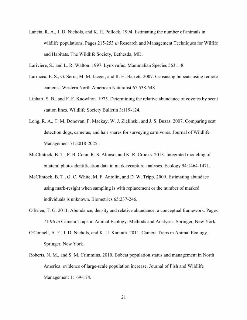
Table 1-1. CMR models for 2016 North Range.

....................................................................................................................................................... 36


....................................................................................................................................................... 36

Table 1-3. CMR models for 2017 both ranges.

....................................................................................................................................................... 37

Table 1-4. Summary of trapping, abundance and density results.

....................................................................................................................................................... 38

Table 1-5. Summary of GPS locations and home range estimates calculated using minimum

convex polygon (MCP) and kernel-density estimation (KDE) methods.

....................................................................................................................................................... 38

Table 2-1. Habitat variables used in a RSF to determine bobcat habitat selection at the capture

point spatial scale. All variables were remotely sensed and combined with “use” and “available”

points using a GIS.

....................................................................................................................................................... 70

Table 2-2. Description of the classes of the SWReGAP land cover data. All of the 22 classes

were used in the capture point scale RSF. The 22 classes were combined into 10 groups that were

used in the home range scale RSF.

....................................................................................................................................................... 70

xiii

Table 2-3. Habitat variables used in a RSF to determine bobcat habitat selection at the home

range spatial scale. All variables were remotely sensed and combined with “use” and “available”

home range buffer polygons using a GIS.

....................................................................................................................................................... 71

Table 2-4. List of 15 topographic variable models comparing bobcat use to available habitat at

both the point and the home range scales.

....................................................................................................................................................... 71

Table 2-5. List of 20 a priory models comparing bobcat use to available habitat using

topographic and land cover variables from both the point and home range scales.

....................................................................................................................................................... 72

Table 2-6. Results of previous research into bobcat habitat suitability.

....................................................................................................................................................... 73

1

CHAPTER 1

Estimating Bobcat Abundance on the Utah Test and Training Range Using Remote Cameras

Kyle Muncey1, Tom Smith1, Steven L. Petersen1, Russ Lawrence2 1Department of Plant and Wildlife Sciences, Brigham Young University, Provo, UT 84602

2Natural Resources Office, Hill Air Force Base, UT 84056

ABSTRACT

Remote cameras have become a popular tool for monitoring wildlife. We used remote

cameras to estimate bobcat (Lynx rufus) population abundance on the Utah Test and Training

Range during two sample periods between 2015 and 2017. We used two statistical methods,

closed capture mark-recapture (CMR) and mark-resight Poisson log-normal (PNE), to estimate

bobcat abundance within the study area. We used the maximum mean distance moved method

(MMDM) to calculate the effective sample area for estimating density. Additionally, we captured

bobcats and estimated home range using minimum convex polygon (MCP) and kernel density

estimation (KDE) methods. Bobcat abundance on the UTTR was 35-48 in 2017 and density was

11.95 bobcats/100 km2 using CMR and 16.69 bobcats/100 km2 using PNE. The North Range of

the study area experienced a decline of 36-44 percent in density between sample periods. Density

declines could be explained by natural predator prey cycles, by habituation to attractants or by an

increase in home range area. We recommend that bobcat abundance and density be estimated

regularly to establish population trends.

INTRODUCTION

Monitoring wildlife species is necessary for a variety of reasons including managing a

species of value for optimal yield, assessing the status of a species of interest, and defining the

health of a particular ecosystem (Witmer 2005). There are many factors to consider when

monitoring animal species. Initially, one should assess what is already known about the species

2

and which methods have been established to monitor them. It is also important to know how

difficult it is to locate and identify individuals. There are three major categories for population

monitoring: census (all animals are seen and counted), incomplete count (samples are counted

and extrapolated to unsampled areas), and indices (derived from an indirect sign such as tracks or

scat; Lancia et al. 1994). Censuses of all members of a population are rarely attempted due to

cost and time constraints, and population indices are discouraged unless it is known how the

indirect sample compares to the population (Lancia et al. 1994). The difficulties involved with

censuses (most species are elusive), and indices (relations between sign and population are

largely unknown and difficult to ascertain), make incomplete counts the most common method

for estimating a population.

Remote cameras are devices equipped with motion sensors that detect and photograph

moving objects within their field of sensitivity. Remote cameras have become the tool of choice

for monitoring wildlife (O'Connell et al. 2011). These cameras are widely used because they

record a photo of each passing object, are easy to operate, are less expensive than human

observers, are less invasive than traditional capture methods, and because they can capture

species and events that are witnessed rarely in person. Many felids are nocturnal, exist at low

density, and are difficult to observe, thus making them prime candidates for remote camera

studies (Heilbrun et al. 2006). Fortunately, many species of felids have pelage markings that are

unique to each individual (Figure 1-1). These natural markings give researchers the advantage of

identifying individuals without handling them (Rowcliffe and Carbone 2008). Bobcats (Lynx

rufus) are an example of a felid that is individually identifiable (Heilbrun et al. 2003).

A commonly used method for population estimation, based on sample data derived from

incomplete counts, is closed capture mark-recapture (CMR; White and Burnham 1999). For this

3

approach, biologists capture animals (a sample), mark them with a distinct identifier, and then

release them. However, several assumptions must be met for this approach to meet statistical

requirements. First, the population must be considered closed. This means that the sampling

period must be sufficiently short and the area sampled must be sufficiently isolated to prevent

births, deaths, immigration and emigration from occurring. Secondly, it is assumed that no

marked individuals were lost during the sample period. Finally, there is an assumption that

marked individuals distribute themselves evenly within the population post-handling. Additional

samples are necessary to increase the accuracy of the abundance estimate. Population estimation

becomes more complex when there are more samples taken and marked. The weaknesses of

CMR are that a remote camera session must be arbitrarily divided into distinct samples and that

an individual may only be counted once in each sample.

A method of estimating abundance using sample data from incomplete counts, that is able

to accommodate a single sample period, is the mark-resight Poisson-log normal method (PNE;

McClintock et al. 2009). The PNE approach must meet the same conditions as CMR (no births,

deaths, immigration, emigration, lost marks or uneven distribution of marks), and individuals are

captured and marked in the same way as CMR. However, with the PNE approach, sampling may

be done with replacement. Replacement refers to an individual being counted more than once in

a recapture period. In PNE the number of times a marked individual is observed during the

remote camera session is counted, rather than counting marked individuals once in arbitrarily

assigned sample periods. Because CMR is restricted to counting an individual only once per

sample, it is possible that some data are not used in the abundance calculation. All recapture data

are used in PNE. Both of these popular methods have been applied to remote camera studies.

Bobcats occur from southern Canada, through the United States and into central Mexico

4

(Figure 1-2; Lariviere and Walton 1997, Sunquist and Sunquist 2002). Though researchers have

studied bobcats throughout much of their range (Ferguson et al. 2009, Roberts and Crimmins

2010), no estimate of abundance (total number of individuals), or density (number of individuals

per unit area) exists for the bobcat population located on the United States Air Force (USAF)

Utah Testing and Training Range (UTTR) in northern Utah. Bobcat sightings, though rare, have

been reported on the UTTR prior to this study (R. Lawrence, Natural Resources Manager Hill

Air Force Base, personal communications). This study was designed to fulfill, in part, the Sikes

Act which requires the Department of Defense, in cooperation with the United States Fish and

Wildlife Service, to develop and implement Integrated Natural Resource Management Plans

(INRMP) which guide the management of military properties (United States Congress 2014). To

meet the Sikes Act criteria, we estimated abundance and density of bobcats on the UTTR.

Bobcats are of additional interest to UTTR managers because they are an apical predator and

indicator species meaning the condition of the bobcat population on the UTTR may be a gauge

of the overall health of the ecosystem.

We used widely accepted methods to assess the status of the population of bobcats on the

UTTR. The objective of this study was to estimate both the abundance and density of bobcats

living on a portion of the UTTR in 2016 and 2017. Because of the elusive nature of bobcats, we

used remote cameras to provide data for both the CMR population estimation method and the

PNE density and abundance method. Additionally, we determined home range of collared

bobcats using minimum convex polygon and kernel density estimation methods, two widely used

methods for determining home range size.

5

METHODS

Description of Study Area

The UTTR is located in the West Desert of Utah 130 km (80 mi) west of Salt Lake City,

Utah (Figure 1-3). The UTTR is directed under the jurisdiction of the USAF Hill Air Force Base

located 160 km (100 mi) to the east near Ogden, Utah. The UTTR is divided into North and

South Ranges, separated by Interstate 80. The North and South Ranges combine for a total of

3,872 km2 (1,495 mi2).

The North Range is bounded by the Great Salt Lake to the east and Bonneville Salt Flats

State Park to the west. It includes portions of the Lakeside, Grassy and Newfoundland

Mountains. The South Range is located between the Cedar Mountains to the east and extends

several kilometers into Nevada to the west. The South Range includes Wildcat Mountain as well

as portions of the Goshute Mountains. Elevation in the study area ranges from 1280 m (4200 ft)

at the shore of Great Salt Lake to 1825 m (5987 ft) in the Newfoundland Mountains.

Temperatures in the study area range from -33°C to 43°C. Annual precipitation averages

19.9 cm, primarily in the form of winter snow. West et al. (2005) described the major ecological

sites within the UTTR including: playas that are predominantly vegetation-free or dominated by

pickleweed (Salicornia europeae), desert vegetated dunes dominated by black greasewood

(Sarcobatus vermiculatus), alkali flats dominated by black greasewood, desert sandy loam

dominated by Indian ricegrass (Stipa hymenoides), and desert loamy soils dominated by

shadscale (Atriplex confertifolia), bluebunch wheatgrass (Pseudoroegneria spicata) and Salina

wildrye (Leymus salinus).

6

Abundance and Density Estimation Using Remote Cameras

Male bobcat home ranges average 1.65 times larger than female home ranges in North

America (Ferguson et al. 2009). Female bobcat home ranges averaged 12-16 km2 and male home

ranges averaged 22-26 km2 in studies conducted near the UTTR (Karpowitz 1981, Frost 1992).

Consequently, we selected a similar sampling grid cell of 10 km2 (3.86 mi2) to sample bobcat

activity. Using geographic information systems, we overlayed this grid layer on over the area

within the UTTR boundary (ArcMap, version 10.5, Environmental Systems Research Institute,

Redlands, California). This grid cell size placed a camera within the estimated home range of

each female bobcat (Zeilinski and Kucera 1995). We assumed that all land cover types were

available for bobcat use except for open water and playa (Figure 1-4). As a result, total available

bobcat habitat where bobcats could occur on the UTTR was estimated at approximately 900 km2.

Using a GPS, we placed remote cameras (Reconyx PC900®) within 500 m of the center of each

grid cell that was not located on open water or playa. As possible, we positioned each camera

near bobcat sign (tracks, scat, latrine, etc.) if found within 500 m of the grid cell center.

We deployed 20 remote cameras from October 2015 through January 2016 on the North

Range of the UTTR (Figure 1-5). Between February and April 2017, we placed 15 remote

cameras on the South Range and 29 remote cameras on the North Range for a total of 44 on the

UTTR (Figure 1-6). Each camera station consisted of a camera placed 50 cm above the ground

facing a wooden stake (25x50x90 mm) with visual and olfactory lures, driven into the soil 2 m

distant (Figure 1-7). Cameras were set to record 5 images per trigger, with no delay between

triggers, and were active 24 hours per day. Each stake was scented by attaching a cotton swab

that was dipped in commercially available bobcat scent lures (Cat Collector®, Predator Control

Group; Montana Magic®, Halseth; Powder River Cat Call®, O’Gorman). Additionally, a dyed

7

turkey (Meleagris spp.) pointer feather was attached to each stake as a visual attractant and to

hold the bobcat’s attention so that the camera could record images for later identification.

Feathers were hung 1 m above the ground by attaching them with fishing line, swivels and wire

(Figure 1-7). We visited each camera weekly to reapply scent bait, ensure proper functioning of

the camera, and download images.

When analyzing photographs of visiting bobcats, we followed previously established

guidelines in an effort to identify each bobcat by comparing pelage spot patterns (Heilbrun et al.

2003). Bobcats are bilaterally asymmetrical with respect to their pelage’ spot pattern (Heilbrun et

al. 2003), which can be problematic when attempting to identify individuals, as occasionally only

one side of the cat was photographed, leaving the other unidentifiable and useless for

identification in subsequent photos. Consequently, researchers have attempted to circumvent this

problem by analyzing right and left side capture histories separately (McClintock et al. 2013,

Alonso et al. 2015). Thornton and Pekins (2015) only classified individuals when both sides had

been photographed. In this study, we attempted to address this problem by not only setting our

cameras to capture 5 images per trigger without delay, thus providing varied angles of the

animal, but also added the dangling feather so that the bobcat would rotate its position providing

a more clear view of each side for more accurate identification. Once individual bobcats were

identified at the various camera stations, we constructed capture histories for each individual

using the time and date of each encounter.

To estimate bobcat abundance, we used CMR and PNE in program MARK (White and

Burnham 1999). Our capture histories for CMR were divided into one week intervals, similar to

the approaches used in previous studies (Larrucea et al. 2007, Clare et al. 2015). Program

MARK uses Akaike’s Information Criterion adjusted for small sample sizes (AICc) to rank

8

models (Akaike 1973). CMR models were constructed within MARK and the top model,

identified by lowest AICc value, was used for further analysis. We used PNE because this

estimator relies on data derived by methods similar to those used in this study. With PNE, we

were able to sample with replacement (i.e., sample an individual multiple times during a

continuous camera sampling period) and do so without knowing the number of marked

individuals in the population, or without having distinct sighting periods (i.e., camera traps were

used as one continuous sighting period). This means that capture histories for PNE included the

number of times an individual was seen during the entire capture period without dividing the

period into arbitrary time intervals as is done in the CMR approach. PNE capture histories

usually include the number of unmarked individuals observed during the capture period, but we

did not have any unmarked individuals because we were able to identify each bobcat

photographed.

We estimated bobcat density within the study area using the mean maximum distance

moved (MMDM) method (Karanth and Nichols 1998, O'Brien 2011). In this method, the mean

distance moved between captures for all bobcats was an estimate of the average home range

diameter. We used the radius of the average home range estimate to create a buffer around all

traps in the grid. Wherever buffers intersected one another, we dissolved them to generate an

effective sample area (Dillon and Kelly 2007). We intersected and joined the resulting area with

available habitat, leaving the area used for estimating density. All geographic data processing

was done using ArcMap. We left bobcats that were captured repeatedly at the same camera,

zero-distance animals, out of the MMDM calculation. Previous research found that including

zero-distance animals increased density estimates and associated standard errors (Dillon and

Kelly 2007). The same study suggested that zero-distance animals should be included only when

9

camera spacing is large relative to the radius of the target animal’s home range. This prevents

inflating buffer values and consequently increasing density estimates.

Home Range Estimation Using GPS Collars

Bobcat trapping and handling was approved by the Utah Division of Wildlife Resources

under a Certificate of Registration (1BAND9745) and by Brigham Young University’s

Institutional Animal Care and Use Committee (protocol number 16-0201). We trapped bobcats

on the UTTR using Havahart® model 1081, Tomahawk® model BC3PK, and #1.75 Oneida

Victor Soft-Catch® double spring foothold traps. We attached foothold traps to a 60 cm chain

that was equipped with two shock-damping springs and two swivels. We anchored foothold traps

to the ground with two stakes. We baited all traps with scent lures (Cat Collector®, Predator

Control Group; Montana Magic®, Halseth; Powder River Cat Call®, O’Gorman). We placed

scent in a small hole beneath cage traps. We also put scent approximately 40 cm above foothold

traps on a nearby rock. Additionally, we rigged a dyed turkey (Meleagris spp.) pointer feather

such that it dangled in the wind, at the back of each cage trap or 1 m above each foothold trap.

We checked all traps before noon each day.

Trapped bobcats were anesthetized in the trap with a 1:1:1 mix of ketamine,

dexmedetomidine (Dexdomitor®), and buprenorphine (Buprenex®). We used a 3 cc syringe pole

to inject drugs intramuscularly. Dexmedetomidine was reversed with atipamezole (Antisedan®).

Dosages were 5 mg/kg, 0.025 mg/kg, 0.15 mg/kg and 0.25 mg/kg respectively. This mixture

allowed for a short period of sedation (20 minutes), but sufficient time to affix a GPS collar

(W300 Wildlink®, Advanced Telemetry Systems). We programmed collars to record bobcat

locations after 12 hours followed by a point after 11 hours. The schedule was repeated so that

10

each hour of the day was sampled in a 12-day period. Collars were equipped with a VHF

transmitter that switched to a mortality signal if no movement was detected after 24 hours. We

weighed the anesthetized bobcat and took reference photos of the tail, inner and outer legs, head,

neck, face and both sides of the body to assist identification during photo-recaptures. After

administering the reversal drug, we placed bobcats inside the trap to recover. We released

bobcats after they had recovered from anesthetization, determined by the bobcat’s ability to

stand, lift, and control its head.

Home range was determined using 95 percent Minimum Convex Polygons (MCP) so that

our results could be directly compared to those of previous studies (Ferguson et al. 2009). We

calculated 95 percent MCP, as well as 50 percent MCP, using the MCP tool within the AniMove

plugin (version 1.4.2) for QGIS (QGIS version 2.18.3, QGIS Development Team, Open Source

Geospatial Foundation Project). This tool removed the outermost 5 percent of GPS locations and

constructed a polygon around the remaining locations. Weaknesses of the 95 percent MCP

include not using the majority of locations when calculating home range area, and that it does not

incorporate relocation density in the home range calculation. We also calculated home range

using the kernel-density estimation method (KDE with hplug-in). This method is considered a more

accurate approach to home range calculation than the traditional MCP method. This method is

appropriate for resident, seasonal animal habitat use, as is the case in our study, and ignores

exploratory animal forays. KDE with hplug-in uses the density of GPS locations to construct an

animal’s home range (Walter et al. 2011). We calculated KDE with hplug-in using the KDE tool

within the AniMove plugin (version 1.4.2) for QGIS (QGIS version 2.18.3, QGIS Development

Team, Open Source Geospatial Foundation Project). This tool allowed us to select the

appropriate value for h (smallest value that produced only one polygon) that encompassed 95

11

percent of the GPS locations within a single polygon. The same h value was used to create a

single polygon that encompassed 50 percent of the GPS locations.

RESULTS

Abundance and Density Estimation Using Remote Cameras

More than 85,000 photos (38 Gigabytes of images) were collected during the two-year

study. A total of 687 and 5199 bobcat images were collected in the 2015-2016 and 2017 periods

respectively. We collected from 5 to 285 photos per bobcat visit and averaged 38 photos per

visit. In the 2015-2016 period, we identified 17 individuals in 30 encounters within the North

Range camera grid. All 20 cameras were active for a total of 1550 trap-nights during the 2015-

2016 period. We encountered bobcats on 12 of the cameras (60 percent). Capture rate was 1.94

encounters/100 trap-nights and recapture rate (individuals seen >1 time) was 29.4 percent (n =

5). In 2017 we identified 33 individuals in 74 encounters across the 44 camera grid (15 on the

South Range and 29 on the North Range). Cameras were active a total of 1781 trap-nights in the

2017 period. We encountered bobcats on 21 of 44 cameras (47.7 percent). Capture rate was 4.15

encounters/100 trap-nights and recapture rate was 54.5 percent (n = 18). For a comparison

between the two years, we used the 20 cameras that were in the same locations in both years. In

2017, this required that we analyze the 20 camera subset separately. In the 2017 subset we

identified 14 individuals in 21 encounters. These 20 cameras were active for 1062 trap-nights.

We encountered bobcats on 8 of 20 cameras (40 percent). Capture rate was 1.98 encounters/100

trap-nights and recapture rate was 42.9 percent (n = 6).

The top CMR model for 2016 (Table 1-1) estimated the population of the North Range to

be 27 bobcats (SE = 6.68) and the top CMR model for 2017 (Table 1-2) estimated the population

12

of the North Range to be 15 bobcats (SE = 2.38). The top model for both ranges in 2017 (Table

1-3) estimated the population to be 35 bobcats (SE = 2.28). PNE estimated the population of the

North Range in 2016 to be 37 bobcats (SE = 12.22) and the population of the North Range in

2017 to be 24 bobcats (SE = 5.36). PNE estimated the population of both the North and South

Range in 2017 to be 48 bobcats (SE = 5.95). A summary of these results is provided in Table 1-

4.

We calculated the mean maximum distance moved (MMDM) from five bobcats that were

captured at more than one camera location. Four of those individuals were captured at two

camera locations and one individual was captured at three camera locations. These bobcats

traveled between 1.5 km and 5 km between cameras. The MMDM calculation resulted in an

average home range radius of 1.59 km. The effective sample area for the 20 cameras sampled in

both years was 132.9 km2. The average home range radius resulted in an effective sample area of

289.8 km2 for 2017 (North and South Ranges; Figure 1-8). Estimated bobcat density of the

effective sample area in 2016 was 20.16 bobcats/100 km2 using CMR and 28.11 bobcats/100

km2 using PNE. Density estimates of the effective sample area for the 2017 subset were 11.36

bobcats/100 km2 using CMR and 18.08 bobcats/100 km2 using PNE. Density estimates for the

effective sample area on the North and South Ranges in 2017 were 11.95 bobcats/100 km2 using

CMR and 16.69 bobcats/100 km2 using PNE. We left 13 zero-distance moved bobcats out of the

MMDM calculation both because our average camera spacing of 2.69 km is relatively similar to

the average home range radius of 1.95-2.26 km (using 12-16 km2 (Karpowitz 1981, Frost 1992)),

and because densities calculated with the zero-distance bobcats were inflated to >11 times

greater than those calculated without the zero-distance bobcats.

13

Home Range Estimation Using GPS Collars

Between May 2016 and June 2017 we trapped for a total of 4160 trap-nights. We

captured 3 individuals (2 male and 1 female). A male was captured on 19 July 2016 and died

from capture-induced hyperthermia. Another male (collar 037264) was captured on 16 August

2016 and tracked until the GPS collar failed on 6 March 2017 with a total of 262 GPS locations.

We calculated the 95 percent MCP for bobcat 037264 to be 17.5 km2 and the 95 percent KDE (h

= 0.4) to be 19.6 km2 (Figure 1-9). The female bobcat (collar 037263) was captured on 24 March

2017 and the GPS collar remains active. However, we used all of the 638 GPS locations between

capture and 13 June 2018 to calculate home range. We calculated the 95 percent MCP for bobcat

037263 to be 40.7 km2 and the 95 percent KDE (h = 0.4) to be 36.3 km2 (Figure 1-10). Bobcat

GPS activity and estimated home ranges are summarized in Table 1-5.

DISCUSSION

We were able to individually identify all bobcats captured in photos through use of the

rapid-fire feature of the Reconyx PC900® cameras and through careful placement of cameras.

Previous studies frequently documented bobcats approaching scent stations at angles that did not

allow pelage markings to be easily seen, or they were only able to photograph one side of the

bobcat. Reconyx’ rapid-fire feature produced approximately two photos for each second that a

bobcat was encountered. Consequently, we collected from 5 to 285 photos per encounter for an

average of 38 photos per encounter. The visual and olfactory lures used also increased the

number of photos per encounter and the angles viewed. This large number of photographs per

encounter made it possible to see both sides of an individual thus aiding identification of

individuals. We positioned cameras perpendicular to game trails, which prevented most bobcats

14

from approaching at odd angles, thus making identification difficult.

Ultimately the accuracy of remote camera surveys is contingent on the number of cells in

the grid, grid cell size, survey duration, and the sampling of all available habitats. Each of these

attributes of the survey should correspond with attributes of the target species. Better estimates

of a species’ abundance are possible with increased survey effort, but there is also a balance

between survey effort and available resources. Research indicates that the number of cameras we

deployed and the number of trap nights we sampled were sufficient to achieve the desired root

mean square error to accurately estimate bobcat abundance on the UTTR. It has been suggested

that the minimum study design for estimating bobcat abundance is one that uses 10 cameras for

60 trap nights (Shannon et al. 2014). For species with high estimates of occupancy and low

estimates of detection probability, as is the case with bobcats, a reduction in error is possible by

increasing the number of trap nights (Shannon et al. 2014). We were only able to camera trap in

certain areas of the UTTR due to military exercises in others. In the absence of those restrictions,

we would have placed cameras in a uniform grid across the entire study area except in open

water and playa. However, we have confidence that the number of cells in our grid was sufficient

because our camera grids on the North and South Ranges were both greater than the minimum

recommended grid of 10 camera traps.

Scent is widely used to attract carnivores (Linhart and Knowlton 1975, Roughton and

Sweeny 1982, Deifenbach et al. 1994), but some debate exists on whether scent attractants

should be used in abundance estimation. Some studies choose not to use scented camera stations

because it may cause heterogeneous capture probability (Heilbrun et al. 2006), skewing capture

towards those individuals most attracted by scent. Though research indicates that visitation of

scent stations is not affected by sex of the bobcat (Deifenbach et al. 1994), scent-station

15

visitation may be affected by the shyness or boldness of individuals and an individual’s

preference for the scents being used (Wilson et al. 1993). Probability of detection, and detection

rates associated with remote cameras are also controversial. Few studies compare remote camera

probability of detection to populations where the abundance is known (Kelly and Holub 2008)

and no such study exists specifically for bobcats.

Though MMDM has been proven reliable with tiger populations, it may underestimate

the home-range size of bobcats as was found with jaguars in Brazil (O'Connell et al. 2011). If

home range size is underestimated, then bobcat density on the UTTR would be over-estimated.

Zero-distance moved animals are problematic because they reduce average home range radius

leading to an over-estimation of density. We feel confident that zero-distance moved bobcats

were appropriately omitted from the MMDM calculation. The effective sample area, when zero-

distance moved bobcats were included, was non-contiguous. Density estimates including zero-

distance moved bobcats were inflated to over 11 times greater than when those bobcats were left

out of the calculation. A literature review of bobcat densities from 24 separate studies indicates

that our density estimates are within the range of reported densities (3-48 bobcats/100 km2;

Thornton and Pekins 2015). However, if zero-distance moved bobcats were included, our

estimates would have been above this range. Other density estimation methods designed

specifically for remote camera and capture-recapture studies, such as spatially explicit capture-

recapture models (Borchers 2012, Efford 2017) and continuous-time spatially explicit capture-

recapture models (Borchers et al. 2014), are currently being developed and used.

The 95 percent home ranges calculated from GPS locations of collared bobcats were

larger than the estimate of home range derived from the MMDM method. The home range

estimated using the MMDM method were closer to the 50 percent core areas of both the MCP

16

and KDE methods than the 95 percent home ranges that we calculated. A literature review

analyzing the home range size of bobcats in 29 studies had only one study with a larger female

bobcat home range estimate than we calculated for bobcat #037263. The home range estimate for

bobcat #037264 falls near the middle, with 10 studies having smaller estimated male home

ranges and 19 studies with larger estimated male home ranges (Ferguson et al. 2009). However,

the collar on bobcat #037264 failed eight months after deployment, so no data were recorded

when this male would have likely expanded its territory significantly in search of mating

opportunities (Lariviere and Walton 1997). If we assume that the two collared bobcats are

representative of other bobcats on the UTTR, then the effective sampling area that we reported in

results using the MMDM method would be larger using either the 95 percent MCP or the 95

percent KDE. This would also cause the densities of bobcats to be lower than we have repored

here.

Bobcats on the UTTR are not hunted and no major environmental change (i.e., extreme

temperatures, drought, floods, etc.), occurred during our research. Therefore, we assume that the

36-44 percent decline we documented in 2017, on the North Range, to be either a natural

population fluctuation or possibly a result of study design. It is likely that bobcats also follow the

example of lynx (Lynx canadensis) populations increasing and decreasing in response to

snowshoe hare (Lepus americanus) populations (Figure 1-11; Elton and Nicholson 1942). Bobcat

populations have been shown to oscillate in response to population cycles of their main prey

sources, black-tailed jackrabbit (Lepus californicus) and cottontail rabbit (Sylvilagus nuttallii). A

northern Utah population of black-tailed jackrabbit was shown to exhibit a 10-year cycle in

population (Keith 1983), and a southeastern Idaho population of bobcats had a decrease in

density (89 percent decrease between 1982 and 1985) as lagomorph populations declined (Knick

17

1990), indicating that this relationship does indeed occur. Historic data on the UTTR show that

its black-tailed jackrabbit population exhibits a similar population cycle (Figure 1-12). This data

also shows that the black-tailed jackrabbit population peaked in 2015 and has since begun to

decline (Figure 1-13; Slater 2016). This coincides with the trend we saw in the bobcat

population. Besides responding numerically to prey abundance, bobcats also increase their home

ranges in search of prey when lagomorph populations decline (Knick 1990). Our study, which

used stationary camera traps, may not be able to detect home range expansion in declining prey

years. Conversely, an actual decline in bobcat density on the UTTR may not be occurring.

Instead, bobcats may have habituated to the scent baits used, having received no positive

reinforcement, and subsequently ceased visiting them.

Remote camera studies require less labor and money than other methods used to monitor

bobcat populations, such as scat detecting dogs (Long et al. 2007). Remote camera studies are

also more successful than hair snaring methods (Harrison 2006). The most expensive aspect of a

remote camera study is the cost of cameras. Nonetheless, for this study, we needed cameras only

for two months of the year, freeing them up for use on other projects for the remainder of the

year on the UTTR. Attractants and cameras are easily deployed and require little training for set

up. After camera/scent bait sites were determined for this study, one person was able to deploy

five camera stations/day on the UTTR. Subsequently, one person was able to check

approximately ten cameras in a day to change memory cards, check batteries and apply new

scent. More than 85,000 photos were collected during the two year study and were stored on a

hard drive. The most time-intensive aspect of remote camera studies is the time spent reviewing

each bobcat encounter and determining which encounters belong to each individual. For this

study, we spent approximately four months working 20 hours each week to identify individual

18

bobcats. The process became easier with practice.

This method for estimating bobcat abundance is relatively easy to implement and cost-

effective, so it can be repeated with regularity. Given our experience on the UTTR, we

recommend that remote camera surveys occur annually during March and April, months of

increased bobcat activity (Heilbrun et al. 2006), to determine the status and trend of this elusive

carnivore on the UTTR. Annual surveys would also help determine if the decline in bobcat

density we estimated was actually occurring. Ideally, bobcat surveys should also be accompanied

by lagomorph surveys to establish predator/prey relationships that may be occurring and

explanatory for changes in bobcat populations. It is possible to design the remote camera survey

in such a way that could determine the status of several target species on the UTTR

simultaneously. Careful consideration would need to be made in determining the number of grid

cells, cell size and survey duration to match the minimum requirements of all target species.

Conclusions drawn from remote camera surveys may be used in conjunction with similar studies

to draw further conclusions about bobcat ecology.

19

WORKS CITED

Akaike, H. 1973. Information theory as an extension of the maximum likelihood principle. Pages

267-281 in B. Petran and F. Csaki, editors. International Symposium on Information

Theory. Second edition. Akademiai Kiado, Budapest, Hungary.

Alonso, R. S., B. T. McClintock, L. M. Lyren, E. E. Boydston, and K. R. Crooks. 2015. Mark-

recapture and mark-resight methods for estimating abundance with remote cameras: a

carnivore case study. Plos One 10:1-13.

Borchers, D. 2012. A non-technical overview of spatially explicit capture-recapture models.

Journal of Ornithology 152:435-444.

Borchers, D., G. Distiller, R. Foster, B. Harmsen, and L. Milazzo. 2014. Continuous-time

spatially explicit capture-recapture models, with an application to jaguar camera-trap

survey. Methods in Ecology and Evolution 5:656-665.

Clare, J. D. J., E. M. Anderson, and D. M. MacFarland. 2015. Predicting bobcat abundance at a

landscape scale and evaluating occupancy as a density index in central Wisconsin.

Journal of Wildlife Management 79:469-480.

Deifenbach, D. R., M. J. Conroy, R. J. Warren, and W. E. James. 1994. A test of the scent-station

survey technique for bobcats. Journal of Wildlife Management 58:10-17.

Dillon, A., and M. J. Kelly. 2007. Ocelot Leopardus pardalis in Belize: the impact of trap

spacing and distance moved on density estimates. Oryx 41:469-477.

Efford, M. 2017. SECR: spatially explicit capture-recapture models.

Elton, C., and M. Nicholson. 1942. The ten-year cycle in numbers of the lynx in canada. Journal

of Animal Ecology 11:215-244.

Ferguson, A. W., N. A. Currit, and F. W. Weckerly. 2009. Isometric scaling in home-range size

20

of male and female bobcats (Lynx rufus). Canadian Journal of Zoology 87:1052-1060.

Frost, G. T. 1992. RAPD DNA analysis and population biology of a Utah bobcat population.

Unpublished M.S. thesis, Brigham Young University, Provo, Utah.

Harrison, R. L. 2006. A comparison of survey methods for detecting bobcats. Wildlife Society

Bulletin 34:548-552.

Heilbrun, R. D., N. J. Silvy, M. J. Peterson, and M. E. Tewes. 2006. Estimating bobcat

abundance using automatically triggered cameras. Wildlife Society Bulletin 34:69-73.

Heilbrun, R. D., N. J. Silvy, M. E. Tewes, and M. J. Peterson. 2003. Using automatically

triggered cameras to individually identify bobcats. Wildlife Society Bulletin 31:748-755.

IUCN (International Union for Conservation of Nature) 2016. Lynx rufus. The IUCN Red List of

Threatened Species. Version 2016.1 http://www.iucnredlist.org. Downloaded on 05 June

2018.)

Karanth, K. U., and J. D. Nichols. 1998. Estimation of tiger densities in India using photographic

captures and recaptures. Ecology 79:2852-2862.

Karpowitz, J. F. 1981. Home ranges and movements of Utah bobcats with reference to habitat

selection and prey base. Unpublished M.S. thesis, Brigham Young University, Provo,

Utah.

Keith, L. B. 1983. Role of food in hare populaiton cycles. Oikos 40:385-395.

Kelly, M. J., and E. L. Holub. 2008. Camera trapping of carnivores: trap success among camera

types and across species and habitat selection by species, on Salt Pond Mountain, Giles

County, Virginia. Northeastern Naturalist 15:249-262.

Knick, S. T. 1990. Ecology of bobcats relative to exploitation and a prey decline in Southeasten

Idaho. Wildlife Monographs 108:3-42.

21

Lancia, R. A., J. D. Nichols, and K. H. Pollock. 1994. Estimating the number of animals in

wildlife populations. Pages 215-253 in Research and Management Techniques for Wilfife

and Habitats. The Wildlife Society, Bethesda, MD.

Lariviere, S., and L. R. Walton. 1997. Lynx rufus. Mammalian Species 563:1-8.

Larrucea, E. S., G. Serra, M. M. Jaeger, and R. H. Barrett. 2007. Censusing bobcats using remote

cameras. Western North American Naturalist 67:538-548.

Linhart, S. B., and F. F. Knowlton. 1975. Determining the relative abundance of coyotes by scent

station lines. Wildlife Society Bulletin 3:119-124.

Long, R. A., T. M. Donovan, P. Mackay, W. J. Zielinski, and J. S. Buzas. 2007. Comparing scat

detection dogs, cameras, and hair snares for surveying carnivores. Journal of Wildlife

Management 71:2018-2025.

McClintock, B. T., P. B. Conn, R. S. Alonso, and K. R. Crooks. 2013. Integrated modeling of

bilateral photo-identification data in mark-recapture analyses. Ecology 94:1464-1471.

McClintock, B. T., G. C. White, M. F. Antolin, and D. W. Tripp. 2009. Estimating abundace

using mark-resight when sampling is with replacement or the number of marked

individuals is unknown. Biometrics 65:237-246.

O'Brien, T. G. 2011. Abundance, density and relative abundance: a conceptual framework. Pages

71-96 in Camera Traps in Animal Ecology: Methods and Analyses. Springer, New York.

O'Connell, A. F., J. D. Nichols, and K. U. Karanth. 2011. Camera Traps in Animal Ecology.

Springer, New York.

Roberts, N. M., and S. M. Crimmins. 2010. Bobcat population status and management in North

America: evidence of large-scale population increase. Journal of Fish and Wildlife


22

Roughton, R. D., and M. W. Sweeny. 1982. Refinements in scent-station methodology for

assessing trends in carnivore populations. Journal of Wildlife Management 46:217-229.

Rowcliffe, J. M., and C. Carbone. 2008. Surveys using camera traps: are we looking to a brighter

future? Animal Conservation 11:185-186.

Shannon, G., J. S. Lewis, and B. D. Gerber. 2014. Recommended survey designs for occupancy

modelling using motion-activated cameras: insights from empirical wildlife data. PeerJ

2:e532; DOI 10.7717/peerj.532.

Slater, S. 2016. West Desert spring 2016 jackrabbit survey results – report for Dugway Proving

Ground. Unpublished Report.

Sunquist, F., and M. Sunquist. 2002. Wild Cats of the World. University of Chicago Press,

Chicago.

Thornton, D. H., and C. E. Pekins. 2015. Spatially explicit capture-recapture analysis of bobcat

(Lynx rufus) density: implications for mesocarnivore monitoring. Wildlife Research

42:394-404.

Walter, W. D., J. W. Fischer, S. Baruch-Mordo, and K. C. VerCauteren. 2011. What is the

proper method to delineate home range of an animal using today’s advanced GPS

telemetry systems: the initial step. in O. Krejcar, editor. Modern Telemetry. InTech,

Online Open Access.

West, N. E., F. L. Dougher, G. S. Manis, and R. R. Douglas. 2005. A comprehensive ecological

land classification for Utah's West Desert. Western North American Naturalist 65:281-

309.

White, G. C., and K. P. Burnham. 1999. Program MARK: Survival estimation from populations

of marked animals. Bird Study 46:120-138.

23

Wilson, D., K. Coleman, A. Clark, and L. Biederman. 1993. Shy-bold continuum in

pumpkinseed sunfish (Lepomis gibbosus): an ecological study of a psychological trait.

Journal of Comparative Psychology 107:250-260.

Witmer, G. W. 2005. Wildlife population monitoring: some practical considerations. Wildlife

Research 32:259-263.

United States Congress. 2014. Sikes Act. Congressional Session 113. Public Law 291.

Zeilinski, W. J., and T. E. Kucera. 1995. American marten, fisher, lynx and wolverine: survey

methods ofr their detection. U. S. Forest Service General Technical Report:17-24.

24

FIGURES

Figure 1-1. Pictures and illustrations of two different bobcats. The inner legs were essential in identifying individuals due to the high contrast between black markings and light colored hair.

25

Figure 1-2. Map showing the distribution of bobcats throughout North America. Geography data from Natural Earth (free vector and raster map data) and distribution data from IUCN (IUCN 2016).

26

Figure 1-3. Location of the study area. The North Range is bounded by Great Salt Lake in the east and Bonneville Salt Flats State Park in the west. It includes portions of the Lakeside, Grassy and Newfoundland Mountains. The South Range is located between the Cedar Mountains in the east and extends several miles into Nevada in the west. It includes Wildcat Mountain as well as portions of the Goshute Mountains.

27

Figure 1-4. We assumed that all land cover types on the UTTR, except open water and playa, were available bobcat habitat. Available habitat (green shaded areas) has an area of 900 km2 within the UTTR boundary.

28

Figure 1-5. We deployed 20 remote cameras from October 2015 through January 2016 on the North Range of the UTTR. Cameras were placed within 500 m of the center of each cell. Cameras were placed near bobcat sign when it was present. The 20 remote cameras deployed from February through April 2017 in these grid cells were placed in the same location as the previous year.

29

Figure 1-6. We deployed 44 remote cameras on the UTTR. This included 15 cameras on the South Range and 29 cameras on the North Range. Cameras were deployed from February through April and were visited weekly to apply new scent, check batteries and download images.

30

Figure 1-7. A Reconyx PC900 remote camera placed 50 cm above the ground and facing a wooden stake (1x2x36 in) 2 m away. Five images were taken each time they were triggered with no delay between triggers and were active 24 hours per day. Attached cotton swabs were dipped in bobcat scent lures (Cat Collector®, Predator Control Group; Montana Magic®, Halseth; Powder River Cat Call®, O’Gorman. Additionally, a dyed, turkey pointer feather was attached as a visual attractant to hold the cat’s attention to obtain more images for identification.

31

Figure 1-8. Each camera was buffered with the 1.59 km average home range radius calculated using MMDM. The resulting buffer was intersected with available bobcat habitat (figure 1-4). The effective sample area of 289.8 km2 for 2017 (North and South Ranges) was then used with abundance estimates to calculate density. Density estimates for the effective sample area on the North and South Ranges in 2017 were 11.95 bobcats/100 km2 using CMR and 16.69 bobcats/100 km2 using PNE.

32

Figure 1-9. This illustrates the home range and core areas of bobcat 037264. Home range was calculated using minimum convex polygon (MCP) and kernel-density estimation (KDE) methods.

33

Figure 1-10. This illustrates the home range and core areas of bobcat 037263. Home range was calculated using minimum convex polygon (MCP) and kernel-density estimation (KDE) methods.

34

Figure 1-11. This illustration was made using data from the trapping numbers of the Hudson Bay Company. It shows the dramatic cycle of the snowshoe hare (Lepus americanus) population and the corresponding cycle of the lynx (Lynx canadensis). Bobcat densities likely oscillate in response to the cycle of their main prey sources. (Image from Pearson Education Inc. 2015)

Figure 1-12. Historic and recent black-tailed jackrabbit (BTJ) density in the West Desert Military Operations Area (MOA) and surrounding areas (Slater 2016).

35

Figure 1-13. Density trends for black-tailed jackrabbits (BTJ) in the Military Operations Area (MOA), 2011-2015.

36

TABLES


Model Model Description AICc ΔAICc AICc Weight

{f0,p(.)=c(.)} Constant capture probability 76.73 0.00 0.67

{f0,p(.),c(.)} Behavioral response 78.70 1.97 0.25

{f0,p(t),c(.)} Varying capture probability and constant recapture probability 80.71 3.98 0.09

{f0,p(.),c(t)} Constant capture probability and varying recapture probability 87.02 10.28 0.00

{f0,p(t)=c(t)} Time varying capture probability 90.66 13.92 0.00








37

Table 1-3. CMR models for 2017 both ranges.







38

Table 1-4. Summary of trapping, abundance and density results.

Individuals Encounters Captures/100 trap-nights

Recapture (seen >1 times) 𝑁𝑁� SE 95% CI Bobcats/100km2

2016 CMR (North) 17 30 1.94 5/17 (29.4%) 27 6.68 19.91-

49.87 20.16

2016 PNE (North) 17 30 1.94 5/17 (29.4%) 37 12.22 20.00-

69.78 28.11

2017 CMR (North) 14 21 1.98 6/14 (42.9%) 15 2.38 14.08-

28.59 11.36

2017 PNE (North) 14 21 1.98 6/14 (42.9%) 24 5.36 15.59-

37.01 18.08

2017 CMR 33 74 4.15 18/33 (54.5%) 35 2.28 33.22-45.53

11.95

2017 PNE 33 74 4.15 18/33 (54.5%) 48 5.95 38.03-61.50

16.69

Table 1-5. Summary of GPS locations and home range estimates calculated using minimum convex polygon (MCP) and kernel-density estimation (KDE) methods.

Collar Sex Start End Relocations 50% MCP 95% MCP 50% KDE 95% KDE h

037263 F 24 March 2017 13 June 2018 638 6.6 km2 40.7 km2 11.1 km2 36.3 km2 0.4

037264 M 16 August 2016 7 March 2017 262 3.6 km2 17.5 km2 6.0 km2 19.6 km2 0.4

39

CHAPTER 2

Modeling Bobcat Habitat Using Remote Cameras on the Utah Test and Training Range

Kyle Muncey1, Tom Smith1, Steven L. Petersen1, Russ Lawrence2 1Department of Plant and Wildlife Sciences, Brigham Young University, Provo, UT 84602

2Natural Resources Office, Hill Air Force Base, UT 84056

ABSTRACT

To improve the management of bobcats on the Utah Test and Training Range (UTTR),

we investigated bobcat (Lynx rufus) habitat use. We determined habitat use points by capturing

bobcats in remote camera images. Use and random points were intersected with remotely sensed

data in a geographic information system. Habitat variables were evaluated at the capture point

scale and home range scale. Home range size was calculated using the mean maximum distance

moved method. Scales and habitat variables were compared within generalized linear mixed-

effects models. Our top model (AICc weight = 1) included a measure of terrain ruggedness, mean

aspect, and land cover variables related to prey availability and human avoidance.

INTRODUCTION

Animal populations inhabit areas which provide the resources necessary for sustenance.

To better understand wildlife-habitat relationships, researchers should identify the resources that

are available and the extent to which those resources are being used (Niedballa et al. 2015). The

idea that animals select one resource over another is the basis for the resource selection function

(RSF). The RSF is a statistical measure of habitat selection used to estimate the probability that

an animal will use a particular resource (Manly et al. 2002). Such information is important in

determining the resource requirements and the impacts that habitat change may have on a

species.

40

Remote cameras are digital devices equipped with motion sensors that detect and

photograph movement within their field of sensitivity. Remote cameras have become the tool of

choice for many researchers in monitoring wildlife populations (O'Connell et al. 2011). These

cameras are popular because they are able to record a photo of each movement, are easy to

operate, are less expensive than human observers, are less invasive than traditional capture

methods, can record tens of thousands of images over long periods of time (~ 6 months), and

capture species and events that are witnessed rarely in person. Many felids, including bobcats

(Lynx rufus), are nocturnal, exist at low density, and are difficult to observe, thus making them

prime candidates for remote camera studies (Heilbrun et al. 2006).

Bobcat locations, as identified by remote camera surveys, have been used to model their

habitat in areas throughout the United States (Preuss and Gehring 2007, Long et al. 2010, Bled et

al. 2015, Halsey et al. 2015, Reed et al. 2016). To model bobcat habitat, the locations of remote

cameras that captured bobcats were compared to habitat variables within a geographic

information system (GIS). GIS gives researchers the ability to intersect multiple habitat variables

with known bobcat locations and identify those site characteristics. Habitat variables may be

remotely sensed or collected in-situ; however, remotely sensed data has the advantage of being

faster and easier to collect over large areas (Niedballa et al. 2015). Habitat selection is scale-

dependent, particularly for carnivores that range widely in search of prey (Mayor et al. 2009).

GIS is essential in analyzing habitat selection at capture site and home range scales because

bobcats may select different habitat variables at these different scales.

Bobcats occur from southern Canada, through the United States and into central Mexico

(Figure 2-1; Lariviere and Walton 1997, Sunquist and Sunquist 2002). Though researchers have

studied bobcats throughout much of their range (Ferguson et al. 2009, Roberts and Crimmins

41

2010), the factors driving habitat selection are unknown for the bobcat population located on the

United States Air Force (USAF) Utah Testing and Training Range (UTTR) in northern Utah

(Figure 2-2). This study was designed to fulfill, in part, the Sikes Act of 1960 which requires the

Department of Defense, in cooperation with the United States Fish and Wildlife Service, to

develop and implement Integrated Natural Resource Management Plans (INRMP) which guide

management of military properties (United States Congress 2014). By estimating bobcat habitat

selection, our study aided in the development and implementation of the INRMP for the UTTR.

To inform management of the UTTR, we modeled bobcat habitat selection at both the capture

point and home range scales. Our objective was to use remote camera captures and remotely

sensed data to assess the resource requirements of bobcats on the UTTR and the effects that

habitat change may have on the distribution of this species.

METHODS

Description of Study Area

The Utah Test and Training Range is located in the West Desert of Utah 130 km (80 mi)

west of Salt Lake City, Utah (Figure 2-2). The UTTR is under the jurisdiction of the USAF Hill

Air Force Base located 160 km (100 mi) to the east, near Ogden, Utah. The UTTR is divided into

North and South Ranges by Interstate 80. The North and South Ranges combine for a total of

3,872 km2 (1,495 mi2).

The North Range is bounded by the Great Salt Lake to the east and Bonneville Salt Flats

State Park to the west. It includes portions of the Lakeside, Grassy and Newfoundland

Mountains. The South Range is located between the Cedar Mountains to the east and extends

several miles into Nevada to the west. The South Range includes Wildcat Mountain as well as

42

portions of the Goshute Mountains. Elevation in the study area ranges from 1280 m (4200 ft) at

the shore of Great Salt Lake to 1825 m (5987 ft) in the Newfoundland Mountains.

Temperatures in the study area range from -33°C to 43°C. Annual precipitation averages

19.9 cm, primarily in the form of winter snow. West et al. (2005) described the major ecological

sites within the UTTR including: playas that are predominantly vegetation free or dominated by

pickleweed (Salicornia europeae), desert vegetated dunes dominated by black greasewood

(Sarcobatus vermiculatus), alkali flat dominated by black greasewood, desert sandy loam

dominated by Indian ricegrass (Stipa hymenoides), desert loam dominated by shadscale (Atriplex

confertifolia), bluebunch wheatgrass (Pseudoroegneria spicata) and Salina wildrye (Leymus

salinus).

Remote Camera Methodology

Male bobcat home ranges average 1.65 times larger than female home ranges (Ferguson

et al. 2009). Female bobcat home ranges were found to average 12-16 km2 in studies conducted

near the UTTR (Karpowitz 1981, Frost 1992). From these data, we selected a grid cell of 10 km2

(3.86 mi2) for sampling bobcat activity. Subsequently, we placed a 10 km2 (3.86 mi2) grid over

the study area using a GIS (ArcMap, version 10.5, Environmental Systems Research Institute,

Redlands, California). This cell size theoretically allowed us to position a camera within the

home range of each female bobcat (Zeilinski and Kucera 1995). We assumed that all land cover

types were available for bobcat selection except for open water and playa (Figure 2-3). As a

result, available bobcat habitat was 900 km2 in extent. We placed remote cameras (Reconyx

PC900®) within 500 m of the center of each grid cell that was not located on open water or playa

and was within 1 km of a road. We determined that we were within 500 m of the center by GPS

43

navigation. We also placed each camera near bobcat sign (tracks, scat, latrine, etc.) if found

within 500 m of the grid cell center.

Following this methodology, we deployed 20 remote cameras from October 2015 through

January 2016 on the North Range of the UTTR (Figure 2-4). Between February and April 2017,

we placed 15 remote cameras on the South Range and 29 remote cameras on the North Range for

a total of 44 on the UTTR (Figure 2-5). Each camera station consisted of a camera placed 50 cm

above the ground and facing a wooden stake (25x50x90 mm) 2 m away (Figure 2-6). Cameras

were set to record 5 images per trigger, with no delay between triggers, and were active 24 hours

per day. The stake was scented by attaching a cotton swab that was dipped in commercially

produced bobcat scent lures (Cat Collector®, Predator Control Group; Montana Magic®, Halseth;

Powder River Cat Call®, O’Gorman). Additionally, a dyed turkey (Meleagris spp.) pointer

feather was attached to the stake as a visual attractant and to hold the bobcat’s attention so that

the camera could record multiple images for later identification. Feathers were made to dangle 1

m off the ground by attaching them to the stake with fishing line, swivel and wire (Figure 2-6).

We visited every camera weekly to reapply scent bait, ensure proper functioning of the camera,

and download images. When analyzing photographs of visiting bobcats, we followed previously

established guidelines in an effort to identify each bobcat by comparing pelage spot patterns

(Heilbrun et al. 2003).

Habitat Variables

Previous studies that modeled bobcat habitat (Woolf et al. 2001) used human population

density, road density, stream density, as well as slope, land cover and other terrain variables. The

UTTR has no permanent human population. Unimproved roads exist on the UTTR, but they are

44

used infrequently and are not likely to affect bobcat use. There are no natural water sources

found on the UTTR and guzzlers are only found on the portion of the UTTR that is on the

Lakeside Mountains. Therefore, only land cover and topographic variables were used in our

analysis (Table 2-1).

Land cover data used in this project was provided by the Southwest Regional Gap

Analysis project (SWReGAP). This data was collected as a multi-institutional effort coordinated

by the United States Geological Survey. The data was derived from Landsat ETM+ images

collected during multiple seasons between 1999 and 2001. The data has a spatial resolution of 30

m and represents 125 vegetation classes (RS/GIS Laboratory et al. 2004). Only 22 classes were

present in our study area (Table 2-2). Elevation data were obtained from the national elevation

dataset, a seamless raster file derived from digitized USGS topo quads with a spatial resolution

of 10 m. Slope, aspect, vector ruggedness measure (VRM), terrain ruggedness index (TRI), and

topographic position index (TPI) were all derived from and have the same spatial resolution as

the elevation raster. Slope and aspect were created using tools available in ArcGIS. TRI and TPI

were calculated using tools available in QGIS 2.18.3 (Quantum GIS Development). TRI is the

mean difference between a central pixel and surrounding cells. TPI is the difference between a

central pixel and the mean of surrounding cells. VRM was calculated by measuring the

dispersion of vectors at right angle to the terrain surface in a designated radius around a central

pixel. This resulted in a value between 0 and 1 that is low in areas that are flat and steep, but high

in areas that are steep and rugged, respectively (Sappington et al. 2007). The location at which

each bobcat encounter occurred was considered a “use” point in a RSF.

In order to model habitat selection at multiple scales, we estimated bobcat home range

within the study area using the mean maximum distance moved (MMDM) method (Karanth and

45

Nichols 1998, O'Brien 2011). In this method, the mean distance moved between captures for all

bobcats was an estimate of the average home range diameter. The radius of the average home

range estimate was used to create a buffer around all “use” points and “available” points (Figure

2-7). All geographic data processing was done using ArcMap®. When calculating the MMDM

values, we omitted data derived from bobcats that were captured repeatedly at the same camera,

zero-distance animals. Previous research found that including zero-distance animals increased

density estimates and their standard errors (Dillon and Kelly 2007). The same study suggested

that zero-distance animals should be included only when camera spacing is large relative to the

radius of the target animal’s home range. This prevents inflating buffer values and consequently

increasing density estimates.

We generated a number of “available” random points (n = 104) equal to the number of

use points. Random points were generated within the habitat available to bobcats on the UTTR.

We assumed that all land cover types were available for bobcat habitat except for open water and

playa (Figure 2-3). We generated random points using the random points tool in a GIS. The

value for each habitat variable was extracted from its raster cell to the “use” points and

“available” points. The mean value of each habitat variable within home range buffers was also

extracted (Table 2-3). Vegetation classes within the SWReGAP layer were each extracted as

percent cover within the home range buffer. For the home range spatial scale, classes were

grouped into 10 categories (Table 2-2) to reduce the number of variables in the RSF. Random

locations must adequately characterize the habitat available to bobcats within the study area. To

determine if such was the case, we calculated the true mean of all pixels within the study area for

each habitat variable and compared results with the random sample mean ± 95 percent

confidence intervals (Westover et al. 2016). The true mean fell within the confidence interval in

46

every case and thus this number was able to adequately represent the availability of habitat in the

study area.

Model Methodology

We used generalized linear mixed-effects models to analyze habitat at two different

scales on the UTTR. We evaluated models using program R 3.4.3 (R Core Team 2017). Habitat

use points were coded as 1 and available points were coded as 0. We included the site of

detection as a random effect while all other variables were fixed effects. Table 2-1 includes a list

of all variables considered at the point scale and Table 2-3 includes a list of all variables

considered at the home range scale. We calculated the Pearson correlation coefficient for each

variable. Highly correlated variables (r > |0.6|) were not used together in the same model. We

scaled all variables prior to analysis. We used a hierarchical approach for determining variables

used in modeling. We first compared the significance of individual variables at both scales. The

scale determined to be more significant in each variable, was used throughout. We then

evaluated topographic variables in 15 candidate models (Table 2-4). The top topographic model

was used in the creation of 20 a priori models (Table 2-5) of what habitat is best suited for

bobcats on the UTTR. A priori models were constructed, in part, using results from previous

research (Table 2-6). Models were compared using Akaike Information Criterion (AIC) values.

We used AICc which has been corrected for use with small data sets.

Coefficients from the top model were used to predict a habitat suitability value for each

180 m x 180 m pixel of vegetated land on the UTTR. This resolution was selected to minimize

computing time, which time increases exponentially with increasingly smaller analysis units.

47

Using a GIS we projected these values across our study area, creating a heat map of bobcat

habitat probability (Figure 2-8).

We used k-fold cross-validation to examine our top model’s ability to predict bobcat

habitat. We divided the data randomly into five groups (k = 5 folds). Each iteration used four of

the groups as training data and one group as test data.

RESULTS

Camera Trapping Grid

We collected > 85,000 photos (38 GB) during the two year study. A total of 687 and

5199 bobcat images were collected in the 2015-2016 and 2017 periods, respectively. We

collected from 5 to 285 photos in a single bobcat encounter and averaged 38 photos per

encounter. In the 2015-2016 period we identified 17 individuals in 30 encounters in the 20

camera grid on the North Range. Cameras were active for a total of 1550 trap-nights in the 2015-

2016 period. We encountered bobcats on 12 of 20 cameras (60 percent). Capture rate was 1.94

encounters/100 trap-nights and recapture rate (individuals seen >1 time) was 29.4 percent (n =

5). In the 2017 period we identified 33 individuals in 74 encounters in the 44 camera grid (15 on

the South Range and 29 on the North Range). Cameras were active for a total of 1,781 trap-

nights in the 2017 period. We encountered bobcats on 21 of 44 cameras (47.7 percent). Capture

rate was 4.15 encounters/100 trap-nights and recapture rate was 54.5 percent (n = 18). All 104

encounters from both trapping periods were used as use points in the RSF

We calculated the mean maximum distance moved (MMDM) from five bobcats that were

captured at more than one camera. Four of those individuals were captured at two cameras and

one individual was captured at three cameras. These bobcats traveled 1.5 km to 5 km between

48

cameras. The MMDM calculation resulted in a home range radius of 1.59 km, or home range

area of 7.94 km2.

Habitat Models

The top model of topography variables (Model 9; AICc weight = 0.99) included VRM

and mean aspect. The top model (Model 8; AICc weight = 1) included VRM, mean aspect, and

the percent cover of the following land cover classifications: developed, dune, invasive,

sagebrush, desert and greasewood. All variables, except the invasive and greasewood land cover

classifications, were significant (P < 0.05). Relative probability of bobcat use increased as VRM

and percent desert increased and decreased as percent developed, percent dunes and percent

sagebrush increased. Relative probability of bobcat use increased with increased mean aspect

between 31 and 283 degrees, indicating that bobcats prefer southerly and westerly slopes on the

UTTR.

Cross-validation indicated that our top model is predictive (P < 0.02). The capture points

of bobcats (n = 104) had 95% (n = 99) in the high category for relative probability of use, 4% (n

= 4) in the medium-high category, and 1% (n = 1) in the medium category. The available

(random) points were distributed relatively evenly across the five categories (25% high, 13%

medium-high, 12% medium, 23% medium-low, and 27% low).

DISCUSSION

Ultimately the accuracy of remote camera surveys depends on the number of cells in the

grid, grid cell size, length of the survey and sampling all available habitats. Each of these survey

attributes should correspond with those of the target species. Better estimates of species’

49

abundance are possible with increased survey effort, but managers must balance cost and benefit

when conducting surveys. Research indicates that the number of cameras we deployed and the

number of trap nights we sampled are sufficient to achieve the desired root mean square error to

estimate abundance for bobcats. It is suggested that the minimum study design for estimating

bobcat abundance is one that uses 10 cameras for 60 trap nights (Shannon et al. 2014). For

species with high estimates of occupancy and low estimates of detection probability, as is the

case with bobcats, a reduction in error is possible by increasing the number of trap nights

(Shannon et al. 2014). We were unable to camera trap in all areas of the UTTR due to military

exercises. In the absence of those restrictions, we would have placed cameras in a uniform grid

across the entire study area except in open water and playa. However, we have confidence that

the number of cells in our grid was sufficient because our camera grids on the north and South

Ranges were both greater than the minimum recommended grid of 10 camera traps.

Scent is widely used to attract carnivores (Linhart and Knowlton 1975, Roughton and

Sweeny 1982, Conner et al. 1983, Deifenbach et al. 1994), but some debate exists on whether it

should be used in abundance estimation. Some studies choose not to use scented camera stations

because it may cause heterogeneous capture probability (Heilbrun et al. 2006), skewing capture

towards those individuals attracted by scent. Though research indicates that visitation of scent

stations is not affected by sex of the bobcat (Deifenbach et al. 1994), scent-station visitation may

be affected by the shyness or boldness of individuals and an individual’s preference for the

scents being used (Wilson et al. 1993). Probability of detection and detection rates when using

remote cameras are also controversial. Few studies compare remote camera probability of

detection to populations where the abundance is known (Kelly and Holub 2008) and no such

study exists specifically for bobcats.

50

Though MMDM has been proven reliable with tiger populations, it may underestimate

the home-range size of bobcats as was found with jaguars in Brazil (O'Connell et al. 2011).

Consequently, if home range size is under-estimated, then bobcat density on the UTTR would be

over-estimated. Zero-distance moved animals are problematic because they reduce average home

range radius leading to over-estimation of density. We feel that removing zero-distance moved

bobcats from the MMDM calculation was appropriate. The effective sample area, when zero-

distance moved bobcats were included, was non-contiguous. Density estimates including zero-

distance moved bobcats were inflated to over 11 times greater than when those bobcats were left

out of the calculation. A literature review of bobcat densities from 24 separate studies indicates

that our density estimates are within the range (3-48 bobcats/100 km2) of known densities

(Thornton and Pekins 2015). However, if zero-distance moved bobcats were included, our

estimates would have been above this range. Other density estimation methods, such as spatially

explicit capture-recapture models (Borchers 2012, Efford 2017) and continuous-time spatially

explicit capture-recapture models (Borchers et al. 2014), designed specifically for remote camera

and capture-recapture studies, are currently being developed and used.

Remote camera studies require less labor and money than other methods used to monitor

bobcat populations, such as scat detecting dogs. Remote camera studies are also more successful

than hair snaring methods (Harrison 2006, Long et al. 2007). The most expensive aspect of a

remote camera study is most often the cost of cameras. Nonetheless, for this study we needed

cameras only for two months of the year and they were used on other projects for the remainder

of the year on the UTTR. Attractants and cameras are easily deployed and require little training

for set up. After camera/scent bait sites were determined for this study, one person was able to

deploy five camera stations/day on the UTTR. Subsequently, one person was able to check

51

approximately ten cameras in a day to change memory cards, check batteries and apply new

scent. We collected > 85,000 photos during the two-year study and were stored on a hard drive.

The most time-intensive aspect of remote camera studies is the time spent reviewing each bobcat

encounter and determining which encounters belong to each individual. For this study, we spent

approximately four months working 20 hours each week to identify individual bobcats. The

process did, however, become easier with practice.

Rock outcroppings are associated with bobcat resting areas. Such was not found true in

southern Illinois where it is supposed that an abundance of vegetative cover served a similar

purpose for cover (Kolowski and Woolf 2002). On the UTTR, VRM was significant in

identifying suitable bobcat habitat. The relative probability of bobcat habitat use increased as

VRM increased (Figure 2-9). VRM, which compares the elevation of each pixel to the elevation

of its neighboring pixels, is high in areas where one would find outcroppings. However, the

SWReGAP land cover data included cliffs as a separate class, and it was not found to be

significant in the models that we compared. The only significant vegetative cover available on

the UTTR are the greasewood and sagebrush land cover classes. Greasewood was included in

our top model, but was not significant (Figure2-16). Sagebrush was a significant factor in our top

model but was negatively correlated with bobcat habitat (Figure 2-14). This means that bobcats

are not selecting for vegetative cover on the UTTR as they do in other ecosystems.

Distance to water was found to be significant in southern Illinois (Kolowski and Woolf

2002). Bobcats in New Hampshire selected forest, shrub and wetlands while avoiding developed

land, agricultural land and open water (Reed et al. 2016). The UTTR does not have any natural

sources of fresh water. Water guzzlers are installed on the North Range but not on the South

Range. Bobcat density was similar in both areas. The “water” land cover class used in our

52

models included saline water and playa. These areas are the lowest elevation on the study area.

We grouped open water and playa because there is very little elevation change across these areas

and the open water periodically rises to cover the entire playa. Elevation did not prove to be

significant in our models nor did the “water” or “wetland” land cover classes. However, the

mean aspect of the home range buffer around each point was significantly and positively

correlated with the relative probability of bobcat habitat between 31 and 283 degrees (Figure 2-

10). This indicates that bobcats prefer southerly and westerly slopes.

Bobcat habitat selection in Michigan was related to road density at both local and home

range spatial scales, but for different reasons at each scale. At the local scale, bobcats were

deterred by increased road density and increased human access. At the community scale, there

was a slight positive correlation between road density and bobcat occupancy. This is likely due

to bobcats using roads to conserve energy, especially to avoid walking in deeper snow (Bled et

al. 2015). Another study in Michigan indicated that bobcats selected for lowland forest and

wetland and were averse to urban areas (Preuss and Gehring 2007). We did not use distance to

roads or road density in any of our models. A small network of roads exists on the UTTR, but

most of the roads within that network are unimproved dirt two-track which are rarely used and

pose no threat to bobcat use. The few improved dirt or paved roads that exist on the UTTR see

fewer than 10 vehicles each day. These may impact bobcat use but only during daylight when

bobcat activity is at its lowest. We used the land cover variable “developed,” which includes

areas used by the military as well as barren land and quarries, as our human avoidance variable.

The “developed” land cover class was negatively correlated with relative probability of bobcat

use (Figure 2-11) indicating that bobcats avoid these areas.

53

The most important factors in bobcat habitat selection in several studies were related to

prey abundance. One study in Michigan concluded that increased road density was related to

areas where timber harvesting had occurred and hare populations were higher (Bled et al. 2015).

The same study concluded that all other significant habitat were related to prey availability. In

Vermont, bobcat habitat selection was slightly correlated with forested wetland, but it was

supposed that these areas were also associated with the highest amount of available prey (Long

et al. 2010). We included land cover groups in our models that represented where bobcat prey

would, and would not be, found. Each land cover group was expressed as percent cover of the

area covered by a home range buffer, calculated using MMDM, and represented several

vegetation classes (Table 2-2). Percent dunes and percent sagebrush were negatively correlated

with relative probability of bobcat use (Figure 2-12 and Figure 2-14). Percent invasive and

percent greasewood were included in our top model, but were not significantly correlated with

relative probability of bobcat use (Figure 2-13 and Figure 2-16). Percent desert was the only

group positively correlated with the relative probability of bobcat use. Lagomorph species

(Lepus californicus, Sylvilagus nuttallii) are frequently targeted by bobcats (Knick et al. 1984),

as are many species of small mammals (Neotoma lepida, Urocitellus townsendii, Peromyscus

maniculatus, Reithrodontomys megalotis). The importance of prey, especially lagomorph

species, is further demonstrated by bobcat populations fluctuating in response to prey population

cycles (Keith 1983, Knick 1990). Black-tailed jackrabbits are opportunistic feeders, but the

majority of their diet is composed of forb and grass species (Wansi et al. 1992). The dune,

sagebrush, invasive and greasewood groups do not contain the forage preferred by lagomorph

species and, therefore, are negatively correlated with or insignificant in determining relative

probability of bobcat use. The desert group contained the desert grassland class in which

54

lagomorph species forage and, therefore, was positively correlated with the likelihood of bobcat

use.

Resource selection may vary based on the scale examined (Manly et al. 2002), therefore

it is important to select a scale that is biologically meaningful to the species being studied

(Preuss and Gehring 2007). Though we were able to evaluate habitat selection at the point and

home range spatial scales, we were only able to evaluate a portion of the temporal scale, October

2015 through January 2016 and February through April in 2017. Temporal scale may be more

important than spatial scale for the habitat selection of bobcats in this area (Mayor et al. 2009).

Prey availability, refuge requirements and reproductive requirements are likely to change

significantly through time. To gain a better perspective of bobcat habitat selection on the UTTR,

we recommend that cameras be deployed for at least a portion of each season throughout the

year.

Producing accurate models for a generalist species such as bobcats is difficult because

they use a wide variety of habitats and because the presence or absence of a bobcat at a particular

location is not certain (Kolowski and Woolf 2002). We were able to use remote cameras to

produce an accurate habitat selection model for a population of bobcats that exists at low density.

Remote camera studies are a less invasive method for estimating habitat selection. This type of

study could also be used to determine species richness at various spatial and temporal scales

(Rovero et al. 2014).

55

WORKS CITED

Bled, F., S. Summers, D. Martell, T. R. Petroelje, D. E. Beyer, and J. L. Belant. 2015. Effects of

prey presence and scale on bobcat resource selection during winter. Plos One

10:e0143347.

Borchers, D. 2012. A non-technical overview of spatially explicit capture-recapture models.

journal of Ornithology 152:435-444.

Borchers, D., G. Distiller, R. Foster, B. Harmsen, and L. Milazzo. 2014. Continuous-time

spatially explicit capture-recapture models, with an application to jaguar camera-trap

survey. Methods in Ecology and Evolution 5:656-665.

Conner, M. C., R. F. Labisky, and D. R. Progulske. 1983. Scent-station indices as measures of

population abundance for bobcats, raccoons, gray foxes and opossums. Wildlife Society


Deifenbach, D. R., M. J. Conroy, R. J. Warren, and W. E. James. 1994. A test of the scent-station

survey technique for bobcats. Journal of Wildlife Management 58:10-17.

Dillon, A., and M. J. Kelly. 2007. Ocelot Leopardus pardalis in Belize: the impact of trap

spacing and distance moved on density estimates. Oryx 41:469-477.

Efford, M. 2017. SECR: spatially explicit capture-recapture models.

Ferguson, A. W., N. A. Currit, and F. W. Weckerly. 2009. Isometric scaling in home-range size

of male and female bobcats (Lynx rufus). Canadian Journal of Zoology 87:1052-1060.

Frost, G. T. 1992. RAPD DNA analysis and population biology of a Utah bobcat population.

Unpublished M.S. thesis, Brigham Young University, Provo, Utah.

Halsey, S. M., W. J. Zeilinski, and R. M. Scheller. 2015. Modeling predator habitat to enhance

reintroduction planning. Landscape Ecology 30:1257-1271.

56

Harrison, R. L. 2006. A comparison of survey methods for detecting bobcats. Wildlife Society


Heilbrun, R. D., N. J. Silvy, M. J. Peterson, and M. E. Tewes. 2006. Estimating bobcat

abundance using automatically triggered cameras. Wildlife Society Bulletin 34:69-73.

Heilbrun, R. D., N. J. Silvy, M. E. Tewes, and M. J. Peterson. 2003. Using automatically

triggered cameras to individually identify bobcats. Wildlife Society Bulletin 31:748-755.

Karanth, K. U., and J. D. Nichols. 1998. Estimation of tiger densities in India using photographic

captures and recaptures. Ecology 79:2852-2862.

Karpowitz, J. F. 1981. Home ranges and movements of Utah bobcats with reference to habitat

selection and prey base. Unpublished M.S. thesis, Brigham Young University, Provo,

Utah.

Keith, L. B. 1983. Role of food in hare populaiton cycles. Oikos 40:385-395.

Kelly, M. J., and E. L. Holub. 2008. Camera trapping of carnivores: trap success among camera

types and across species and habitat selection by species, on Salt Pond Mountain, Giles

County, Virginia. Northeastern Naturalist 15:249-262.

Knick, S. T. 1990. Ecology of bobcats relative to exploitation and a prey decline in Southeasten

Idaho. Wildlife Monographs 108:3-42.

Knick, S. T., S. J. Sweeny, J. R. Alldredge, and J. D. Brittell. 1984. Autumn and winter food

habits of bobcats in Washington state. Great Basin Naturalist 44:70-74.

Kolowski, J. M., and A. Woolf. 2002. Microhabitat use by bobcats in Southern Illinois. Journal

of Wildlife Management 66:822-832.

Lariviere, S., and L. R. Walton. 1997. Lynx rufus. Mammalian Species 563:1-8.

57

Linhart, S. B., and F. F. Knowlton. 1975. Determining the relative abundance of coyotes by scent

station lines. Wildlife Society Bulletin 3:119-124.

Long, R. A., T. M. Donovan, P. Mackay, W. J. Zeilinski, and J. S. Buzas. 2010. Predicting

carnivore occurrence with noninvasive surveys and occupancy modeling. Landscape

Ecology 26:327-340.

Long, R. A., T. M. Donovan, P. Mackay, W. J. Zielinski, and J. S. Buzas. 2007. Comparing scat

detection dogs, cameras, and hair snares for surveying carnivores. Journal of Wildlife


Manly, B. F. J., L. L. McDonald, D. L. Thomas, T. L. McDonald, and W. P. Erickson. 2002.

Resource selection by animals. Kluwer Academic Publishers, Dordrecht, Netherlands.

Mayor, S. J., D. C. Schneider, J. A. Schaefer, and S. P. Mahoney. 2009. Habitat selection at

multiple scales. Écoscience 16:238-247.

Niedballa, J., R. Sollmann, A. B. Mohamed, J. Bender, and A. Wilting. 2015. Defining habitat

covariates in camera-trap based occupancy studies. Scientific Reports 5:1-10.

O'Brien, T. G. 2011. Abundance, density and relative abundance: a conceptual framework. Pages

71-96 in Camera Traps in Animal Ecology: Methods and Analyses. Springer, New York.

O'Connell, A. F., J. D. Nichols, and K. U. Karanth. 2011. Camera traps in animal ecology.

Springer, New York.

Preuss, T. S., and T. M. Gehring. 2007. Landscape analysis of bobcat habitat in the northern

lower peninsula of Michigan. Journal of Wildlife Management 71:2699-2706.

R Core Team. 2017. Version 3.2.4. Vienna, Austria.

58

Reed, G. C., J. A. Litvaitis, M. Ellingwood, P. Tate, D. J. A. Broman, A. P. K. Siren, and R. P.

Carrol. 2016. Describing habitat suitability of bobcats (Lynx rufus) using several souces

of information obtained at multiple spatial scales. Mammalian Biology 82:17-26.

Roberts, N. M., and S. M. Crimmins. 2010. Bobcat population status and management in North

America: evidence of large-scale population increase. Journal of Fish and Wildlife


Roughton, R. D., and M. W. Sweeny. 1982. Refinements in scent-station methodology for

assessing trends in carnivore populations. Journal of Wildlife Management 46:217-229.

Rovero, F., E. Martin, M. Rosa, J. A. Ahumada, and D. Spitale. 2014. Estimating species

richness and modelling habitat preferences of tropical forest mammals from camera trap

data. Plos One 9:e103300.

RS/GIS Laboratory, College of Natural Resources, and Utah State University. 2004. Digital

landcover dataset fro the Southwestern United States. USGS GAP Analysis Program.

Sappington, J. M., K. M. Longshore, and D. B. Thompson. 2007. Quantifying landscape

ruggedness for animal habitat analysis: a case study using bighorn sheep in the mojave

desert. Journal of Wildlife Management 71:1419-1426.

Shannon, G., J. S. Lewis, and B. D. Gerber. 2014. Recommended survey designs for occupancy

modelling using motion-activated cameras: insights from empirical wildlife data. PeerJ

2:e532.

Sunquist, F., and M. Sunquist. 2002. Wild cats of the world. University of Chicago Press,

Chicago.

59

Thornton, D. H., and C. E. Pekins. 2015. Spatially explicit capture-recapture analysis of bobcat

(Lynx rufus) density: implications for mesocarnivore monitoring. Wildlife Research

42:394-404.

United States Congress. 2014. Sikes Act. Congressional Session 113. Public Law 291.

Wansi, T., R. D. Pieper, R. F. Beck, and L. W. Murray. 1992. Botanical content of black-tailed

jackrabbit diets on semidesert rangeland. Great Basin Naturalist 52:300-308.

West, N. E., F. L. Dougher, G. S. Manis, and R. R. Douglas. 2005. A comprehensive ecological

land classification for Utah's West Desert. Western North American Naturalist 65:281-

309.

Westover, M., J. Baxter, R. Baxter, C. Day, R. Jensen, S. Petersen, and R. T. Larsen. 2016.

Assessing greater sage-grouse selection of brood-rearing habitat using remotely-sensed

imagery: can readily available high-resolution imagery be used to identify brood-rearing

habitat across a broad landscape? Plos One 11:e0156290.

Wilson, D., K. Coleman, A. Clark, and L. Biederman. 1993. Shy-bold continuum in

pumpkinseed sunfish (Lepomis gibbosus): an ecological study of a psychological trait.

Journal of Comparative Psychology 107:250-260.

Woolf, A., C. K. Neilsen, T. Weber, and T. J. Gibbs-Kieninger. 2001. Statewide modeling of

bobcat, Lynx rufus, habitat in Illinois, USA. Biological Conservation 104:191-198.

Zeilinski, W. J., and T. E. Kucera. 1995. American marten, fisher, lynx and wolverine: survey

methods for their detection. U. S. Forest Service General Technical Report:17-24.

60

FIGURES

Figure 2-1. Map showing the distribution of bobcats throughout North America. Geography data from Natural Earth (free vector and raster map data) and distribution data from IUCN (IUCN 2016).

61

Figure 2-2. Location of the study area. The North Range is bounded by Great Salt Lake in the east and Bonneville Salt Flats State Park in the west. It includes portions of the Lakeside, Grassy and Newfoundland Mountains. The South Range is located between the Cedar Mountains in the east and extends several miles into Nevada in the west. It includes Wildcat Mountain as well as portions of the Goshute Mountains.

62

Figure 2-3. We assumed that all land cover types on the UTTR, except open water and playa, were available bobcat habitat. These land cover types have an area of 900 km2on the UTTR.

63

Figure 2-4. We deployed 20 remote cameras from October 2015 through January 2016 on the North Range of the UTTR. Cameras were placed within 500 m of the center of each cell. Cameras were placed near bobcat sign when it was present. The 20 remote cameras deployed from February through April 2017 in these grid cells were placed in the same location as the previous year.

64

Figure 2-5. We deployed 44 remote cameras on the UTTR. This included 15 cameras on the South Range and 29 cameras on the North Range. Cameras were deployed from February through April and were visited weekly to apply new scent, check batteries and download images.

65

Figure 2-6. A Reconyx PC900 remote camera placed 50 cm above the ground and facing a wooden stake (1x2x36 in) 2 m away. Five images were taken each time they were triggered with no delay between triggers and were active 24 hours per day. Attached cotton swabs were dipped in bobcat scent lures (Cat Collector®, Predator Control Group; Montana Magic®, Halseth; Powder River Cat Call®, O’Gorman. Additionally, a dyed, turkey pointer feather was attached as a visual attractant to hold the cat’s attention to obtain more images for identification.

66

Figure 2-7. Use points are camera locations that captured a bobcat. Available points are random points within available bobcat habitat and the study area. We assumed that all land cover types except open water and playa were available bobcat habitat.

67

Figure 2-8. Map showing the predicted habitat suitability across the UTTR. Only vegetated areas were used in the prediction.

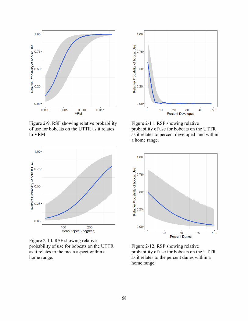
68

Figure 2-9. RSF showing relative probability of use for bobcats on the UTTR as it relates to VRM.

Figure 2-10. RSF showing relative probability of use for bobcats on the UTTR as it relates to the mean aspect within a home range.

Figure 2-11. RSF showing relative probability of use for bobcats on the UTTR as it relates to percent developed land within a home range.

Figure 2-12. RSF showing relative probability of use for bobcats on the UTTR as it relates to the percent dunes within a home range.

69

Figure 2-13. RSF showing relative probability of use for bobcats on the UTTR as it relates to the percent of invasive species within a home range.

Figure 2-14. RSF showing relative probability of use for bobcats on the UTTR as it relates to the percent sagebrush within a home range.

Figure 2-15. RSF showing relative probability of use for bobcats on the UTTR as it relates to the percent desert within a home range.

Figure 2-16. RSF showing relative probability of use for bobcats on the UTTR as it relates to the percent of greasewood within a home range.

70

TABLES

Table 2-1. Habitat variables used in a RSF to determine bobcat habitat selection at the capture point spatial scale. All variables were remotely sensed and combined with “use” and “available” points using a GIS. Variable Name Description Topographic NED10m Elevation in meters NED10mSlop Slope in degrees NED10mAspe Azimuth of aspect NED10mVRM Vector Ruggedness Measure (with default 3-cell neighborhood) NED10mTRI Terrain Ruggedness Index (with default 3-cell neighborhood) NED10mTPI Topographic Position Index (with default 3-cell neighborhood) Land Cover SWReGAP Land cover classes (see Table 2-2 for class descriptions)

Table 2-2. Description of the classes of the SWReGAP land cover data. All of the 22 classes were used in the capture point scale RSF. The 22 classes were combined into 10 groups that were used in the home range scale RSF. Pixel Value Description Group 8 Inter-Mountain Basins Cliff and Canyon Cliff 11 Inter-Mountain Basins Active and Stabilized Dune Dune 14 Inter-Mountain Basins Playa Water 30 Rocky Mountain Montane Dry-Mesic Mixed Conifer Forest and

Woodland Montane

37 Great Basin Pinyon-Juniper Woodland Montane 41 Rocky Mountain Gambel Oak-Mixed Montane Shrubland Montane 48 Inter-Mountain Basins Big Sagebrush Shrubland Sagebrush 49 Great Basin Xeric Mixed Sagebrush Shrubland Sagebrush 58 Inter-Mountain Basins Mixed Salt Desert Scrub Desert 67 Inter-Mountain Basins Semi-Desert Shrub Steppe Desert 71 Southern Rocky Mountain Montane-Subalpine Grassland Montane 76 Inter-Mountain Basins Semi-Desert Grassland Desert 82 Inter-Mountain Basins Greasewood Flat Greasewood 85 North American Arid West Emergent Marsh Wetland 98 Great Basin Lower Montane Riparian Woodland and Shrubland Wetland 110 Open Water Water 111 Developed, Open Space – Low Intensity Developed 113 Barren Lands, Non-specific Developed 117 Recently Mined or Quarried Developed 119 Invasive Perennial Grassland Invasive 121 Invasive Annual Grassland Invasive 122 Invasive Annual and Biennial Forbland Invasive

71

Table 2-3. Habitat variables used in a RSF to determine bobcat habitat selection at the home range spatial scale. All variables were remotely sensed and combined with “use” and “available” home range buffer polygons using a GIS. Variable Name Description Topographic NED10m_mean Mean elevation value in meters, in home range buffer NED10mAspe_mean Mean azimuth of aspect, in home range buffer NED10mSlop_mean Mean slope in degrees, in home range buffer NED10mTPIP_mean Mean Topographic Position Index value in home range buffer NED10mTRI_mean Mean Terrain Ruggedness Index value in home range buffer NED10mVRM_mean Mean Vector Ruggedness Measure value in home range buffer Land Cover Dune Percent dune in home range buffer (see Table 2-2 for classes) Developed Percent developed in home range buffer (see Table 2-2 for classes) Invasive Percent invasive in home range buffer (see Table 2-2 for classes) Water Percent water in home range buffer (see Table 2-2 for classes) Sagebrush Percent sagebrush in home range buffer (see Table 2-2 for classes) Montane Percent montane in home range buffer (see Table 2-2 for classes) Desert Percent desert in home range buffer (see Table 2-2 for classes) Cliff Percent cliff in home range buffer (see Table 2-2 for classes) Greasewood Percent greasewood in home range buffer (see Table 2-2 for

classes) Wetland Percent wetland in home range buffer (see Table 2-2 for classes)

Table 2-4. List of 15 topographic variable models comparing bobcat use to available habitat at both the point and the home range scales. Model Structure 1 Use ~ (1|TrapSite) + NED10m 2 Use ~ (1|TrapSite) + NED10mSlop 3 Use ~ (1|TrapSite) + NED10mAspe_mean 4 Use ~ (1|TrapSite) + NED10mVRM 5 Use ~ (1|TrapSite) + NED10mTRI 6 Use ~ (1|TrapSite) + NED10mTPI 7 Use ~ (1|TrapSite) + NED10mAspe_mean + NED10m 8 Use ~ (1|TrapSite) + NED10mAspe_mean + NED10mSlop 9 Use ~ (1|TrapSite) + NED10mAspe_mean + NED10mVRM 10 Use ~ (1|TrapSite) + NED10mAspe_mean + NED10mTRI 11 Use ~ (1|TrapSite) + NED10mAspe_mean + NED10mTPI 12 Use ~ (1|TrapSite) + NED10mTPI + NED10m 13 Use ~ (1|TrapSite) + NED10mTPI + NED10mSlop 14 Use ~ (1|TrapSite) + NED10mAspe_mean + NED10mTPI + NED10m 15 Use ~ (1|TrapSite) + NED10mAspe_mean + NED10mTPI + NED10mSlop

72

Table 2-5. List of 20 a priory models comparing bobcat use to available habitat using topographic and land cover variables from both the point and home range scales. Model Structure 1 Use ~ (1|TrapSite) + NED10mVRM + NED10mAspe-mean + SWReGAP 2 Use ~ (1|TrapSite) + NED10mVRM + NED10mAspe-mean + Cliffs 3 Use ~ (1|TrapSite) + NED10mVRM + NED10mAspe-mean + Sagebrush + Montane

+ Greasewood4 Use ~ (1|TrapSite) + NED10mVRM + NED10mAspe-mean + Water + Wetland 5 Use ~ (1|TrapSite) + NED10mVRM + NED10mAspe-mean + Developed 6 Use ~ (1|TrapSite) + NED10mVRM + NED10mAspe-mean + Dune + Invasive

+Sagebrush + Desert + Greasewood7 Use ~ (1|TrapSite) + NED10mVRM + NED10mAspe-mean + Sagebrush + Montane

+ Greasewood + Developed8 Use ~ (1|TrapSite) + NED10mVRM + NED10mAspe-mean + Developed + Dune +

Invasive + Sagebrush + Desert + Greasewood 9 Use ~ (1|TrapSite) + NED10mVRM + NED10mAspe-mean + Sagebrush + Montane

+ Greasewood + Dune + Invasive + Desert10 Use ~ (1|TrapSite) + NED10mVRM + NED10mAspe-mean + Sagebrush + Montane

+ Greasewood + Water + Wetland + Developed11 Use ~ (1|TrapSite) + SWReGAP 12 Use ~ (1|TrapSite) + Cliffs 13 Use ~ (1|TrapSite) + Sagebrush + Montane + Greasewood 14 Use ~ (1|TrapSite) + Water + Wetland 15 Use ~ (1|TrapSite) + Developed 16 Use ~ (1|TrapSite) + Dune + Invasive +Sagebrush + Desert + Greasewood 17 Use ~ (1|TrapSite) + Sagebrush + Montane + Greasewood + Developed 18 Use ~ (1|TrapSite) + Developed + Dune + Invasive + Sagebrush + Desert +

Greasewood 19 Use ~ (1|TrapSite) + Sagebrush + Montane + Greasewood + Dune + Invasive +

Desert 20 Use ~ (1|TrapSite) + Sagebrush + Montane + Greasewood + Water + Wetland +

Developed

73

Table 2-6. Results of previous research into bobcat habitat suitability. Study Study Area Characteristics of bobcat habitat (Halsey et al. 2015) Washington, USA Selected low elevation forests with large diameter

trees (Kolowski and Woolf 2002)

Illinois, USA Selected areas of high cover at 1-2 m above ground and high understory stem density.

(Reed et al. 2016) New Hampshire, USA

Selected for vegetative cover and avoided developed areas and open water

(Bled et al. 2015) Michigan, USA Selected areas of high prey abundance and avoided areas of high road density

(Long et al. 2010) Vermont, USA Selected areas of mixed forest and forested wetland (Preuss and Gehring 2007)

Michigan, USA Selected lowland forest, non-forested wetland and streams.

Documents

Bobcat Abundance and Habitat Selection on the Utah Test