Blind motion deblurring using multiple images

Jian-Feng Caia,∗, Hui Jib,∗, Chaoqiang Liua, Zuowei Shenb

aCenter for Wavelets, Approx. and Info. Proc., National University of Singapore,

Singapore, 117542bDepartment of Mathematics, National University of Singapore, Singapore, 117542

Abstract

Recovery of degraded images due to motion blurring is one challenging problemin digital imaging. Most existing techniques on blind deblurring are not capa-ble of removing complex motion blurring from the blurred images of complexstructures. One promising approach is to recover the clear image using multipleimages captured for the scene. However, it is observed in practice that such amulti-frame approach can recover a high-quality clear image of the scene only af-ter multiple blurred image frames are accurately aligned during pre-processing,which is a very challenging task even with user interactions. In this paper, byexploring the sparsity of the motion blur kernel and the clear image under cer-tain domains, we proposed an alternative iteration approach to simultaneouslyidentify the blur kernels of given blurred images and restore a clear image. Ourproposed approach not only is robust to image formation noises, but also isrobust to the alignment errors among multiple images. A modified version oflinearized Bregman iteration is then developed to efficiently solve the resultingminimization problem. The experiments showed that our proposed algorithmis capable of accurately estimating the blur kernels of complex camera motionswith minimal requirements on the accuracy of image alignment. As a result,our method is capable of automatically recovering a high-quality clear imagefrom multiple blurred images.

Key words: blind deconvolution, tight frame, motion blur, image restoration

1. Introduction

Motion blurring caused by camera shake has been one of the prime causes ofpoor image quality in digital imaging, especially when using telephoto lenses orlong shuttle speeds. In many imaging applications, there is simply not enoughlight to produce a clear image by using a short shutter speed. As a result, theimage will appear blurry due to the relative motion between the camera and the

∗Corresponding author. Tel.: +65-65168845, Fax: +65-67795452Email addresses: tslcaij@nus.edu.sg (Jian-Feng Cai), matjh@nus.edu.sg (Hui Ji),

tslcql@nus.edu.sg (Chaoqiang Liu), matzuows@nus.edu.sg (Zuowei Shen)

Preprint submitted to Elsevier March 4, 2010

scene. Motion blurring can significantly degrade the visual quality of images.Thus, how to restore motion-blurred images has long been a fundamental prob-lem in digital imaging. Motion blurring due to camera shake is usually modeledas a spatially invariant convolution process:

f = g ∗ p+ n, (1)

where ∗ is the convolution operator, g is the clear image to recover, f is theobserved blurred image, p is the blur kernel (or so-called point spread function),and n is the noise. How to recover the clear image g from the blurred image fis the so-called image deconvolution problem.

There are two cases in image deconvolution problems: non-blind deconvolu-tion and blind deconvolution. In the non-blind case, the blur kernel p is assumedto be known or estimated somewhere else, and the task is to recover the clearimage g by reversing the effect of convolution on the blurred image f . Such adeconvolution is known as an ill-conditioned problem, as a small perturbation onf may cause the direct solution from (1) being heavily distorted. In past, therehave been extensive studies on robust non-blind deconvolution algorithms (e.g.[1, 22, 8, 7, 18]). In the case of blind deconvolution, both the blur kernel p andthe clear image g are unknown. Then the problem becomes under-constrainedand there exist infinitely many solutions. In general, blind deconvolution ismuch more challenging than non-blind deconvolution. Motion deblurring is atypical blind deblurring problem, because the motion between the camera andthe scene always varies for different images.

Some prior assumptions on both the kernel p and the image g have to bemade in order to eliminate the ambiguities between the kernel and the image.In practice, the motion-blur kernel is very different from the kernels of othertypes of blurring (e.g. out-of-focus blurring, Gaussian-type optical blurring),as there exist not simple parametric forms to represent motion-blur kernels. Ingeneral, the motion-blur kernel can be expressed as

p = v(x, y)|C , (2)

where C is a continuous curve of finite length in R2 which denotes the camera

trajectory and v(x, y) is the speed function which varies along C. Briefly, themotion-blur kernel p is a smooth function with the support of a continuouscurve.

1.1. Previous work

Early works on motion deblurring usually use only one single blurred image.Most such methods (e.g. [10, 29, 21, 17]) require a prior parametric knowledgeof the blur kernel p such that the blur kernel can be obtained by only esti-mating a few parameters. These methods usually are computationally efficientbut only work on simple blurrings such as symmetric optical blurring or sim-ple motion blurring of constant velocity. To remove more complicated blurringfrom images, an alternative approach is using a joint minimization model to

2

simultaneously estimate both the blur kernel and the clear image. To overcomethe inherent ambiguities between the blur kernel and the clear image, certainregularization terms have to be added in the minimization, e.g., total variation(TV) regularization proposed by [9, 8, 16, 20]. These TV-based blind decon-volution techniques showed good performance on removing certain blurrings onspecific types of images, such as out-of-focus blurring on medical images andsatellite images. However, TV regularization is not a good choice for the case ofmotion-blurring, because TV regularization penalizes, e.g., the total length ofthe edges for piecewise constant functions (see [8]). As a result, the support ofthe resulting blur kernel tends to be a disk or several isolated disks, instead ofa continuous curvy camera trajectory. Also, for many images of nature scenes,TV-based regularization does not preserve the details and textures very well onthe regions of complex structures due to the stair-casing effects (see [13, 23]).

In recent years, the concept of epsilon photography ([27]) has been popularin digital imaging to optimize the digital camera by recording the scene viamultiple images, captured by an epsilon variation on the camera setting. Thesemultiple images make a more complete description on the scene, which leads toan easier configuration for many traditionally challenging image processing tasksincluding blind motion deblurring. Most such approaches (e.g. [3, 26, 28, 19])actively control the capturing process using specific hardwares to obtain multipleimages of the scene such that the blur kernel is easier to infer and the deblurringis also more robust to noise. Impressive results have been demonstrated by theseapproaches. However, the requirement on the active acquisition of input imageslimits the wider applications of these techniques in practice.

1.2. Our work

The goal of this paper is to develop a robust numerical algorithm to recovera high-quality clear image of the scene from multiple motion-blurred images. Inour setting, the input multiple images are passively captured by a commoditydigital camera without any specific hardware. It is noted that the proposedalgorithm could also be applied to removing motion blurring in the video withlittle modifications. In other words, as the input in our algorithm, there are Mavailable blurred images with the following relationships:

{fi = g(hi(·)) ∗ pi + ni, i = 1, 2, · · · ,M},

where hi is the spatial geometric transform from the clear image g to the blurredimage fi, determined by the camera pose when the i-th image is taken, pi is theblur kernel of the i-th image, and ni is the noise.

In this paper, we assume the geometric transforms his among all images areestimated using some existing image alignment technique during pre-processing.However, we emphasize that there is no available image alignment techniquewhich is capable of accurately aligning blurred images. Therefore, we take thefollowing fis as the input in our mathematical formulation:

{fi = g((I + ǫhi)(·)) ∗ pi + ni, i = 1, 2, · · · ,M}, (3)

3

where I is the identical operator, pi and g are unknowns, ǫhi and ni are align-ment errors and image formation noises respectively. In summary, there are twotypes of undesired perturbations when taking a multi-image approach to removemotion blurring. One is the image formation noise ni and the other is imagealignment error ǫhi. The goal of this paper is to develop a numerical algorithmrobust to both types of perturbations.

In this paper, we begin our study on blind motion deblurring by investigatinghow to measure the “clearness” of the recovered image and on the “soundness”of the blur kernel. Our study shows that, given multiple images (≥ 2), thesparsity of image under tight frame systems ([12, 30]) is a good measurementon the “clearness” of the recovered image, and the sparsity of blur kernels ina weighted image space is a good measurement on the “soundness” of the blurkernel when combined with a smoothness regularization. In particular, it isshown empirically that the impressive robustness to image alignment error isachieved by using these two sparsity regularizations on restoring the clear imageand on estimating the blur kernels. In our proposed approach, the sparsity of animage under a tight frame system is the ℓ1-norm of its tight frame coefficients,and the sparsity of a blur kernel in a weighted image space is measured by itsweighted ℓ1-norm.

The rest of the paper is organized as follows. In Section 2, we formalizedthe minimization strategy and explained the underlying motivation. In Section3, we presented the detailed numerical algorithm for solving the proposed min-imization problem. Section 4 is devoted to the experimental evaluation and thediscussion on future works.

2. Problem formulation and analysis

When taking an image by a digital camera, the image does not represent thescene in a single instant of time, instead it represents the scene over a periodof time. As the camera does not keep still due to unavoidable camera shake,the image of the scene must represent an integration of all camera viewpointsover the period of exposure time, which is determined by the shuttle speed.The resulted image will look blurry along the relative motion path between thecamera and the scene. As the relative motion between the scene and the cam-era is generally global; usually we assume that the relative motion is spatiallyinvariant. Thus the motion blurring is simplified as a convolution process:

f = g ∗ p+ n, (4)

where p is so-called blur kernel function which represents the relative motionwith normalization, f is the observed blurred image and g is the desired clearimage.

2.1. Benefits of using multiple images

The benefits of using multiple images to remove motion blurring are two-folded. First, it is known that non-blind deblurring is an ill-conditioned problem

4

as it is sensitive to noises. The noise sensitivity comes from the fact that re-versing image blurring process will greatly amplify the high-frequency noise

contribution to the recovered image. Let (·) denote the Fourier transform, then(1) becomes

p(ω) · g(ω) = f(ω) − n.

The values of |p| are zero or very small at large ω because the blur kernel p usu-ally is a low-pass filter. Thus, g(ω) is very sensitive to even small perturbationsat large ω. Extensive studies have been carried out in past to reduce such noisesensitivities by imposing some extra regularizations.

However, if we have multiple perfectly aligned images fi on the same scenewith different motion-blur kernels:

fi = pi ∗ g + ni, i = 1, 2, · · · ,M. (5)

Because motion-blur kernels are not isotropic, the intersection of all ω with small|pi(ω)| is very likely to be much smaller than the set of ω with small |pi(ω)| foreach individual pi. Let us examine a simple example of two blurred images: oneis blurred by a horizontal filter p1 = 1

N (1, 1, · · · , 1); the other is blurred by avertical filter p2 = 1

N (1, 1, · · · , 1)T . Then we have

p1(ωx, ωy) = sinc(2

Nωx); p2(ωx, ωy) = sinc(

2

Nωy).

p1 has the periodic lines of zero points {(ωx = kNπ2 , ωy), k ∈ Z} and so

does p2. However, the combination of p1 and p2 only has periodic points{(ωx = kNπ

2 , ωy = kNπ2 ), k ∈ Z}, which can greatly improve the condition

of the deconvolution process. In practice, we may not have such an ideal con-figuration. But it is very likely that different blurred images have different blurkernels, as the camera motion is random during the capture. Heuristically, it isa reasonable assumption that the combination of all blur kernels

(

N∑

i=1

|pi|2(ω))12 .

will have much fewer small values in its spectrum than the individual blur kerneldoes. Therefore, using multiple images can greatly improve the noise sensitivityof the deconvolution process.

Secondly, for blind deblurring, the estimation of blur kernels will benefiteven more by using multiple images. The main difficulty in blind deblurring isthat the problem is under-constrained. There exist infinitely many solutions.For example, the famous degenerate solution to (4)

p := δ, g := f.

has been a headache for many blind deblurring techniques. Although the de-generate solution can be avoided by some ad-hoc processes, the inherent ambi-guities between the kernel and the image still lead to the poor performance ofmost available techniques on removing complex motion blurring from images.

5

However, such ambiguities can be significantly reduced by using multipleimages. Again, let us examine one example. In the case of a single image, letthe blur kernel be decomposed into two parts: p = p1 ∗ p2. Then besides thetrue solution (p, g), (p1, p2 ∗ g) is also a solution to (4). As long as p2 is a low-pass filter, even imposing other available physical constraints on images or blurkernels, e.g.,

p ≥ 0;∑

j,k

p(j, k) = 1; g ≥ 0, (6)

will not eliminate such ambiguities. On the contrary, in the case of multipleimages, it is very unlikely that such ambiguities will happen. In order to haveanother solution to the system (5) when using multiple images, all N kernels pineed to have a common factor p2 such that

pi = p1i∗ p2.

Considering the fact that the support of each pi is a curve in 2D, it is unlikelythat all pi will have a non-trivial common factor.

In summary, multiple blurred images on the same scene provide much moreinformation than a single blurred image does, which leads to a better config-uration for recovering a clear image on the scene. But, some new challengingcomputational problems also arise when taking a multi-frame approach.

2.2. Challenges of using multiple images

When we take multiple images on the same scene, the camera pose variesduring the capture. In other words, we have multiple observed blurred imagefi related to the clear picture g up to a spatial geometrical transform hi:

{fi = g(hi(·)) ∗ pi + ni, i = 1, 2, · · · ,M}.

The estimation on hi is known as the image registration problem, which hasbeen extensively studied in past (see [34] for more details). However, most imageregistration techniques need to assume a simple model (e.g. affine transform)on the geometrical transform, which may not approximate the true geometricaltransform well when the 3D structure of the scene is complicated. Furthermore,when images are seriously blurred, the appearances of the same scene blurredby different blur kernels are very different from each other. Currently theredoes not exist an alignment technique which is capable of accurately aligningseriously blurred images. Therefore, we have a new perturbation source whenusing multiple images: image alignment error.

It is observed in [19] that alignment errors will seriously impact the perfor-mance of multi-image blind deblurring. In [19], a simple experiment is carriedout to illustrate the high sensitivity of blind deblurring to alignment errors whenestimating blur kernels. The experiment considered a simplified configurationby assuming knowing the clear image and the blurred image up to a small align-ment perturbation. The only unknown is the blur kernel. Thus, the inputs ofthe experiment are a clear image g shown in Fig. 1 (a) and its blurred version

6

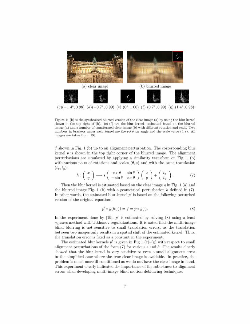
(a) clear image (b) blurred image

(c)(−1.4◦, 0.98) (d)(−0.7◦, 0.99) (e) (0◦, 1.00) (f) (0.7◦, 0.99) (g) (1.4◦, 0.98).

Figure 1: (b) is the synthesized blurred version of the clear image (a) by using the blur kernelshown in the top right of (b). (c)-(f) are the blur kernels estimated based on the blurredimage (a) and a number of transformed clear image (b) with different rotation and scale. Twonumbers in brackets under each kernel are the rotation angle and the scale value (θ, s). Allimages are taken from [19].

f shown in Fig. 1 (b) up to an alignment perturbation. The corresponding blurkernel p is shown in the top right corner of the blurred image. The alignmentperturbations are simulated by applying a similarity transform on Fig. 1 (b)with various pairs of rotations and scales (θ, s) and with the same translation(tx, ty):

h :

(xy

)−→ s

(cos θ sin θ− sin θ cos θ

) (xy

)+

(txty

). (7)

Then the blur kernel is estimated based on the clear image g in Fig. 1 (a) andthe blurred image Fig. 1 (b) with a geometrical perturbation h defined in (7).In other words, the estimated blur kernel p′ is based on the following perturbedversion of the original equation:

p′ ∗ g(h(·)) = f = p ∗ g(·). (8)

In the experiment done by [19], p′ is estimated by solving (8) using a leastsquares method with Tikhonov regularizations. It is noted that the multi-imageblind blurring is not sensitive to small translation errors, as the translationbetween two images only results in a spatial shift of the estimated kernel. Thus,the translation error is fixed as a constant in the experiment.

The estimated blur kernels p′ is given in Fig 1 (c)–(g) with respect to smallalignment perturbations of the form (7) for various s and θ. The results clearlyshowed that the blur kernel is very sensitive to even a small alignment errorin the simplified case where the true clear image is available. In practice, theproblem is much more ill-conditioned as we do not have the clear image in hand.This experiment clearly indicated the importance of the robustness to alignmenterrors when developing multi-image blind motion deblurring techniques.

7

3. Formulation for blind motion deblurring with sparsity regulariza-

tions

3.1. Outline of our proposed algorithm

Given M blurred images fi, i = 1, 2, · · · ,M satisfying the relationship (3):

fi = g((I + ǫhi)(·)) ∗ pi + ni, i = 1, 2, · · · ,M,

we take a regularization-based approach to solve the blind motion deblurringproblem, which requires the simultaneous estimations on both the clear image gand M blur kernels {pi, i = 1, · · · ,M}. It is well known that the regularization-based blind deconvolution approaches usually result in solving a challengingnon-convex minimization problem. In our case, the number of the unknowns isup to the order of millions. The most commonly used approach is an alternativeiteration scheme; see [9] for instance. The alternative iteration scheme can bedescribed as following: let g(0) be the initial guess on the clear image.

Algorithm 1 Outline of the alternative iterations

For k = 0, 1, · · · ,

1. given the clear image g(k), compute the blur kernels {p(k+1)i , i =

1, 2, . . . ,M}.

2. given the blur kernels {p(k+1)i , i = 1, 2, . . . ,M}, compute the clear image

g(k+1);

There are two steps in Algorithm 1. Step 2 is a non-blind image deblurringproblem, which has been studied extensively in the literature; see, for instances,[1, 22, 8, 7, 18, 5]. However, there is one more error source in Step 2 thanthe traditional non-blind deblurring problem does, that is, the error in the in-

termediate blur kernel p(k+1)i used for deblurring. Inspired by recent non-blind

deblurring techniques which are based on the sparse approximation to the imageunder certain tight frame systems ([7, 4]), we also use the sparsity constrainton the clear image g under tight frame systems to regularize the non-blind de-blurring. And we use a modified version of so-called linearize Bregman iteration(See [24, 32, 31, 16, 20, 11, 25, 4, 5, 6, 15]) to achieve impressive robustnessto image noises, alignment errors, and, more importantly, the perturbations onthe given intermediate blur kernels. In our implementation, we choose the tightframelet system constructed in [12, 30] as the choice of the tight frame systemrepresenting the clear image g.

For Step 1, it is observed in Fig. 1 that the alignment error will lead to afalse estimation on the motion blur kernel. The support of the false kernel tendsto be much larger than that of the true blur kernel. Based on this observation,we propose to overcome the sensitivity of estimating blur kernels to alignmenterrors by exploring the sparsity constraint on the motion blur kernel in its

8

spatial domain. Similarly, we also use a modified version of linearized Bregmaniteration to solve the resulting minimization problem. Before we present thedetailed algorithm, we give a brief introduction to the framelet system used inour method in the remaining of the section.

3.2. Tight framelet system and image representation

A countable set X ⊂ L2(R) is called a tight frame of L2(R) if

f =∑

h∈X〈f, h〉h, ∀f ∈ L2(R), (9)

where 〈·, ·〉 is the inner product of L2(R). An orthonormal basis is a tight frame,hence a tight frame is a generalization of an orthonormal basis. However, tightframes sacrifice the orthonormality and the linear independence of the systemin order to get more flexibilities. Tight frames can be redundant.

For given Ψ := {ψ1, . . . , ψr} ⊂ L2(R), the affine (or wavelet) system isdefined by the collection of the dilations and the shifts of Ψ as

X(Ψ) := {ψℓ,j,k : 1 ≤ ℓ ≤ r; j, k ∈ Z} with ψℓ,j,k := 2j/2

ψℓ(2j · −k). (10)

When X(Ψ) forms a tight frame of L2(R), it is called a tight wavelet frame, andψℓ, ℓ = 1, . . . , r, are called the (tight) framelets.

To construct a set of framelets, usually, it starts with a compactly supportedrefinable function φ ∈ L2(R) (a scaling function) with a refinement mask τφsatisfying

φ(2·) = τφφ.

Here φ is the Fourier transform of φ, and τφ is a trigonometric polynomial withτφ(0) = 1, i.e., a refinement mask of a refinable function must be a lowpassfilter. For a given compactly supported refinable function, the construction oftight framelet systems is to find a finite set Ψ that can be represented in theFourier domain as

ψ(2·) = τψφ

for some 2π-periodic τψ. The unitary extension principle (UEP) of [30] saysthat X(Ψ) in (10) generated by Ψ forms a tight frame in L2(R) provided thatthe masks τφ and {τψ}ψ∈Ψ satisfy:

τφ(ω)τφ(ω + γπ) +∑

ψ∈Ψ

τψ(ω)τψ(ω + γπ) = δγ,0, γ = 0, 1 (11)

for almost all ω in R. τφ must correspond to a low-pass filter and {τψ}ψ∈Ψ

must correspond to highpass filters. The sequences of Fourier coefficients ofτψ, as well as τψ itself, are called framelet masks. In our implementation, weadopt piece-wise linear B-spline framelet constructed in [12, 30]. The refinementmask is τφ(ω) = cos2(ω2 ), whose corresponding lowpass filter is h0 = 1

4 [1, 2, 1].

9

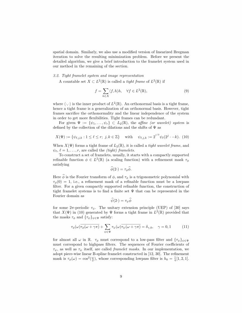
Figure 2: Piecewise linear framelets.φ ψ

1ψ

2

Two framelets are τψ1= −

√2i2 sin(ω) and τψ2

= sin2(ω2 ), whose correspondinghighpass filters are

h1 =

√2

4[1, 0,−1], h2 =

1

4[−1, 2,−1].

The associated refinable function and framelets are given in Fig. 2. With a 1Dframelet system for L2(R), the 2D framelet system for L2(R

2) can be easilyconstructed by the tensor product of 1D framelet.

In the discrete case, an n×n image f is considered as the coefficients {f(i) =〈f, φ(·−i)〉, i ∈ Z

2} up to a dilation, where φ is the refinable function associatedwith the framelet system, and 〈·, ·〉 is the inner product in L2(R

2). The L-leveldiscrete framelet decomposition of f is then the coefficients {〈f, 2−L/2φ(2−L ·−j)〉, j ∈ Z

2} at a prescribed coarsest level L, and the framelet coefficients

{〈f, 2−l/2ψi(2−l · −j)〉, j ∈ Z2, 1 ≤ i ≤ r2 − 1},

for 0 ≤ l ≤ L.If we denote f as a vector f ∈ R

N , N = n2 by concatenating all columnsof the image, the discrete framelet decomposition of f can be described by thevector Af , where A a K × N matrix. By the UEP (11), ATA = I, thus therows of A form a tight frame system in R

N . In other words, the frameletdecomposition operator A can be viewed as a tight frame system in R

N as itsrows form a tight frame in R

N such that the perfect reconstruction formulax =

∑y∈A〈x,y〉y holds for all x ∈ R

N . Unlike the orthonormal case, we

emphasize that AAT 6= I in general. In our implementation, we use a multi-level tight framelet decomposition without down-sampling under the Neumann(symmetric) boundary condition. The detailed description can be found in [7].

4. Numerical algorithm

This section is devoted to the detailed numerical algorithm of our blinddeconvolution algorithm outlined in Algorithm 1. Both steps in Algorithm 1are based on the linearized Bregman iteration. The Bregman iteration was firstintroduced for non-differentiable TV-energy in [24], and then was successfullyapplied to ℓ1-norm minimization in compressed sensing in [32] and to waveletbased denoising in [31]. The Bregman iteration was also used in TV-based blind

10

deconvolution in [16, 20]. To further improve the performance of the Bregmaniteration, a linearized Bregman iteration was invented in [11]; see also [32].More details and an improvement called “kicking” of the linearized Bregmaniteration was described in [25], and a rigorous theory was given in [4, 6]. Thelinearized Bregman iteration for frame-based image deblurring was proposedin [5]. Recently, a new type of iteration based on Bregman distance, calledsplit Bregman iteration, was introduced in [15], which extended the utility ofBregman iteration and linearized Bregman iteration to minimizations of moregeneral ℓ1-based regularizations including total variation, Besov norms and sumsof such things.

Consider M blurred images fi ∈ RN , i = 1, · · · ,M . We assume that the size

of the blur kernel is no larger than n×n. Let pi ∈ RN denote the blurred image

pi after column concatenation. Let [ ]∗ denote the convolution operator of p andf after concatenating operation:

p ∗ f = [p]∗f = [f ]∗p.

Let u = Ag denote the framelet coefficients vector of the clear image g.

4.1. Method for Step 2 in Algorithm 1

In Step 2 of Algorithm 1, at the k-th iteration, we need to find a clear image

g(k+1) given the blur kernels {p(k+1)i , i = 1, 2, · · ·M}.

In the initial stages, since the kernel is not in good shape, it is not necessaryto find an accurate g(k+1). We simply use a least squares deblurring algorithm,i.e., solve

ming

1

2

M∑

i=1

‖[p(k+1)i ]∗g − fi‖2

2 + λ‖∇g‖22. (12)

This can be done efficiently by FFTs.In the final stages, the kernel becomes in good shape, so we need an accurate

solution of the clear image. For this, we solve the image deblurring problem inthe tight framelet domain. Let u be the tight framelet coefficients of the clearimage g(k+1), i.e., gk+1 = ATu. Our strategy of recovering the clear imageg(k+1) is to find a sparse solution u in the tight framelet domain among allsolutions with reasonable constraints.

Temporarily, we ignore the mis-alignment error and assume that the blurkernels are accurate enough, such that there exist solutions for the equations

[p(k+1)i ]∗A

Tu = fi, i = 1, 2, · · · ,M.

To seek a sparse set of coefficient u, we need to minimize its ℓ1-norm ‖u‖1.Thus, we have to solve

minu

‖u‖1

subject to [p(k+1)i ]∗(ATu) = fi, i = 1, 2, · · · ,M.

(13)

11

The linearized Bregman iteration is a very efficient tool to solve the aboveminimization problem. Given x(0) = v(0) = 0, the linearized Bregman iterationgenerates a sequence of x(l) and v(l) as follows

{v(l+1) = v(l) − ∑M

i=1AP(k+1)i [p

(k+1)i ]T∗

([p

(k+1)i ]∗(ATx(l)) − fi

),

x(l+1) = 1ν2Tµ2

(vl+1).(14)

Here Tµ2is the soft-thresholding operator defined by

Tµ2(v) = [tµ2

(v1), tµ2(v1), . . .], with tµ2

(vi) = sign(vi) max(|vi| − µ2, 0),

and P(k)i is a preconditioning matrix to accelerate the convergence of the itera-

tion. Usually, we choose

P(k+1)i =

([p

(k+1)i ]T∗ [p

(k+1)i ]∗ + τ2∆

)−1, (15)

where ∆ is the discrete Laplacian. Notice that the operators P(k+1)i and [p

(k+1)i ]T∗

are commutable since they are all entrywise multiplications in the Fourier do-main.

The basic idea of the linearized Bregman iteration (14) for finding a sparsesolution is as follows. Two steps are involved in the linearized Bregman iteration.The first step is to find an approximate solution (a least squares solution in ourcase) to the residual equation of the constraint in (13) to update the data.However, the updated data may not be sparse. Therefore, the second step, asoft-thresholding operator, is applied to obtain a sparse framelet coefficients set.The procedure is repeated and it converges to a sparse solution in the frameletdomain. The algorithm is efficient and robust to noises as analyzed by [5] andwe also have the following convergence results from [5]. See [4, 5, 6, 32] for amore detailed analysis.

Proposition 1. Assume that there exists at least one solution of {[p(k+1)i ]∗(ATu) =

fi, ∀ i = 1, 2, . . . ,M}. Then, there exists a constant c such that, for allν2 ∈ (0, c), the sequence x(l) generated by (14) converges to the unique solu-tion of

minu

‖u‖1 + 12µ2ν2

‖u‖22

subject to [p(k+1)i ]∗(ATu) = fi, i = 1, 2, · · · ,M.

(16)

Therefore, if we choose a sufficiently large thresholding parameter µ, then theiteration (14) converges to a solution of (13).

During the iterations of Algorithm 1, the intermediate results of the blurkernels are not accurate until the last few iterations. More importantly, there arealignment errors among the observed images. Thus, to obtain a good deblurredimage, one can still use (13), but need to stop it early when the error of theconstraint in (13) satisfies

‖[p(k+1)i ]∗(A

Tu) − fi‖22 ≤ δ22 , i = 1, 2, · · ·M, (17)

12

where δ22 is an estimation of the variance of the image noises, the inaccuracy ofthe blur kernels, and the image alignment errors. The main reason is that theBregman iteration has a good property: in the sense that the Bregman distancedecreases, x(l) approaches the tight frame coefficients of the true image untilthe residual in the iteration drops below the variance of the errors, as showntheoretically in [24, 32]. Furthermore, (14) is very robust to image noises andalignment errors in fi ([5]).

In summary, in Step 2 of Algorithm 1, we use the linearized Bregman itera-tion (14) with the stopping criteria (17) to get a clear image. Usually, it takesonly tens of iterations for (14) to get an image of satisfactory visual quality.

4.2. Method for Step 1 in Algorithm 1

In Step 1 of Algorithm 1, given the intermediate clear image g(k), we want

to compute the blur kernels {p(k+1)i , i = 1, 2, · · ·M}. As shown in (2), a true

motion blur kernel can be approximated well by a smooth function with thesupport of a continuous curve. It is observed that there are two essential prop-erties of a “sound” motion blur kernel: one is the overall smoothness of the blurkernel; the other is its curvy support which implies its sparsity in spatial do-main. Inspired by this observation, we model the motion blur kernel as a sparsesolution in spatial domain with strong smoothness on its support. Thus, the

proposed algorithm is to find the sparse blur kernels {p(k+1)i , i = 1, 2, . . . ,M}

in spatial domain subject to certain smoothness constraints, which results in anℓ1 norm minimization problem. In order to further improve the accuracy andthe efficiency of estimating the blur kernel, we use a weighted ℓ1 norm insteadthe ordinary one.

Same as our previous discussions on Step 1, temporarily, we ignore the imagealignment errors and assume that the clear image are accurate enough, such thatthere exist solutions for the equations

[g(k)]∗pi = fi, i = 1, 2, · · · ,M.

Since a weighted ℓ1-norm is minimized, we have to solve

argminpi

‖Wipi‖1, subject to [g(k)]∗pi = fi, i = 1, 2, · · · ,M, (18)

where Wi is the diagonal weighting matrix. Again, the linearized Bregmaniteration can be applied to solve (18). The iteration is as follows, starting from

r(0)i = q

(0)i = 0,

{r(l+1)i = r

(l)i −Q(k)[g(k)]T∗

([g(k)]∗q

(l)i − fi

),

q(l+1)i = 1

ν1WiTµ1

((Wi)

−1rl+1i

).

(19)

Here Tµ1is the soft-thresholding operator, Q(k) is a preconditioner matrix:

Q(k) =([g(k)]T∗ [g(k)]∗ + τ1∆

)−1,

13

where ∆ is the discrete Laplacian. Again, Q(k) and [g(k)]T∗ are commutable.Similar to Proposition 1, (19) gives a sparse solution and we have the conver-gence of (19).

Proposition 2. Assume that there exists at least one solution of [g(k)]∗pi =fi, ∀ i = 1, 2, . . . ,M . Then, there exists a constant c such that, for all ν1 ∈ (0, c),

the sequence q(l)i generated by (19) converges to the unique solution of

minpi

‖Wipi‖1 + 12µ1ν1

‖pi‖22

subject to [g(k)]∗pi = fi, i = 1, 2, . . . ,M.(20)

Therefore, if we choose a sufficiently large thresholding parameter µ1, then theiteration (19) converges to a solution of (18).

During the iterations of Algorithm 1, the intermediate result of the clearimage is not accurate and there are alignment errors among the observed images.Similar to the method for Step 2, we still use (19), but stop it early when theerror of the constraint satisfies

‖[g(k)]∗qli − fi‖2

2 ≤ δ21 , (21)

where δ21 is an estimation of the variance of the errors caused by the noise, the

inaccuracy of the clear image and the alignment errors. Therefore, q(l)i generated

by (19), with a large µ1 and stopping criteria (21), gives a good estimation ofthe blur kernel. From our empirical observations, only a couple of iterationsalready yield a satisfactory estimation on the blur kernel.

From Proposition 2, (19) minimizes the ℓ2 norm of the blur kernel amongall the minimal weighted ℓ1 norm solutions (See [4, 5, 6] for details). We wouldlike to explain more on why (19) is likely to yield a blur kernel which is asmooth function with a curvy support. In the first step of (19), the opera-

tion Q(k)[g(k)]T∗

([g(k)]∗q

(l)i − fi

)essentially yields the solution of the following

minimization:

minpi

1

2‖[g(k)]∗pi − t

(k)i ‖2 + τ1‖∇pi‖2,

where t(k)i is the residual of the i-th observed image at the k-th step satisfying

t(k)i = [g(k)]∗q

(l)i − fi.

In other words, a Tikhonov regularization with the penalty ‖∇pi‖2 is appliedin the preconditioning step. Thus, the smoothness of the estimated blur kernelis imposed to better constrain the smoothness of the blur kernel pi. The sideeffect is that the resulting blur kernel tends to spread out of the true support dueto the smoothing. Therefore, the second step of (19) comes in to remove thisside effect by finding a sparse solution with minimal weighted ℓ1 norm from theprevious one, which is done by applying a soft-thresholding operator as shownin (19). The support of the resulting sparse solution is then shrunken and likelyto approximate the true support better than the previous one.

14

If only using the Tikhonov regularization, the resulting blur kernel will bea smooth function with the support of a large region; if only using the sparsityconstraint, the resulting blur kernel will be very likely to converge to the de-generate case of only a few isolated points. By balancing the smoothness of thekernel using a Tikhonov regularization and the sparsity of the kernel in spatialdomain using a weighted ℓ1 norm, the sequence generated from (19) will con-verge as Proposition 2 proved. And the resulting solution will be close to theideal motion blur kernel model, that is, a smooth function with the support ofa continuous curve.

How to choose an appropriate Wi is dependent on the support of the trueblur kernel p∗

i . A good example of Wi is

Wi(m,m) =

{ 1|p∗i (m)| , if p∗

i (m) 6= 0

∞, otherwise;and Wi(m,n) = 0, if m 6= n,

for j, k = 1, · · · , N . Unfortunately, It is impossible to construct such a Wi

without knowing the blur kernel pi. In our approach, we take a simple algorithmwhich updates the weighting matrix Wis iteratively. That is, during the k-th

iteration for the blur kernel estimation, we define the weighting matrix W(k)i as

such

W(k)i (m,n) =

{(|([a]∗p

(k)i )(m)| + ǫ)−1, if m = n

0, otherwise,

based on the value p(k)i obtained from the last iteration. Here [a]∗ is the con-

volution with a local average kernel. The weighting matrix W(k)i will be used

in the next iteration. The parameter ǫ is to avoid numerical instability. It isobserved empirically that such a weighting ℓ1 norm can greatly speed up thealgorithm.

4.3. The Complete Algorithm

Due to all types of noises and errors, the numerical algorithms do not alwaysyield a solution which satisfies the physical rules of the image in the digitalworld. In order to obtain a physical solution, we also impose the followingphysical conditions:

{pi ≥ 0,

∑j pi(j) = 1, i = 1, 2, · · · ,M.

g = Atu ≥ 0.(22)

The constraints (22) say that all pixel values of the recovered image has tobe non-negative, and the estimation kernel should also be non-negative and itssummation should be 1. It is noted that the physical constraint on the kernelpi partially explains the reason why the regular ℓ1 norm is not a good sparsitymeasurement on the kernel pi because the ℓ1 norm of the kernel pi is always 1 ifpi satisfies the constraints (22). Combining all together, the complete algorithmfor our blind deconvolution is described in Algorithm 2.

15

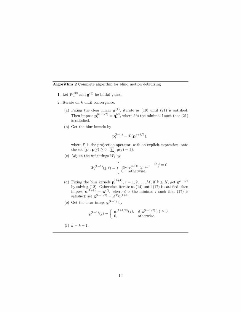
Algorithm 2 Complete algorithm for blind motion deblurring

1. Let W(0)i and g(0) be initial guess.

2. Iterate on k until convergence.

(a) Fixing the clear image g(k), iterate as (19) until (21) is satisfied.

Then impose p(k+1/2)i = q

(ℓ)i , where ℓ is the minimal l such that (21)

is satisfied.

(b) Get the blur kernels by

p(k+1)i = P(p

k+1/2i ),

where P is the projection operator, with an explicit expression, ontothe set {p : p(j) ≥ 0,

∑j p(j) = 1}.

(c) Adjust the weightings Wi by

W(k+1)i (j, ℓ) =

{1

|([a]∗p(k+1)i )(j)|+ǫ

, if j = ℓ

0, otherwise.

(d) Fixing the blur kernels p(k+1)i , i = 1, 2, . . . ,M , if k ≤ K, get gk+1/2

by solving (12). Otherwise, iterate as (14) until (17) is satisfied; thenimpose u(k+1) = x(ℓ), where ℓ is the minimal l such that (17) issatisfied; set g(k+1/2) = ATu(k+1).

(e) Get the clear image g(k+1) by

g(k+1)(j) =

{g(k+1/2)(j), if g(k+1/2)(j) ≥ 0;0, otherwise.

(f) k = k + 1.

16

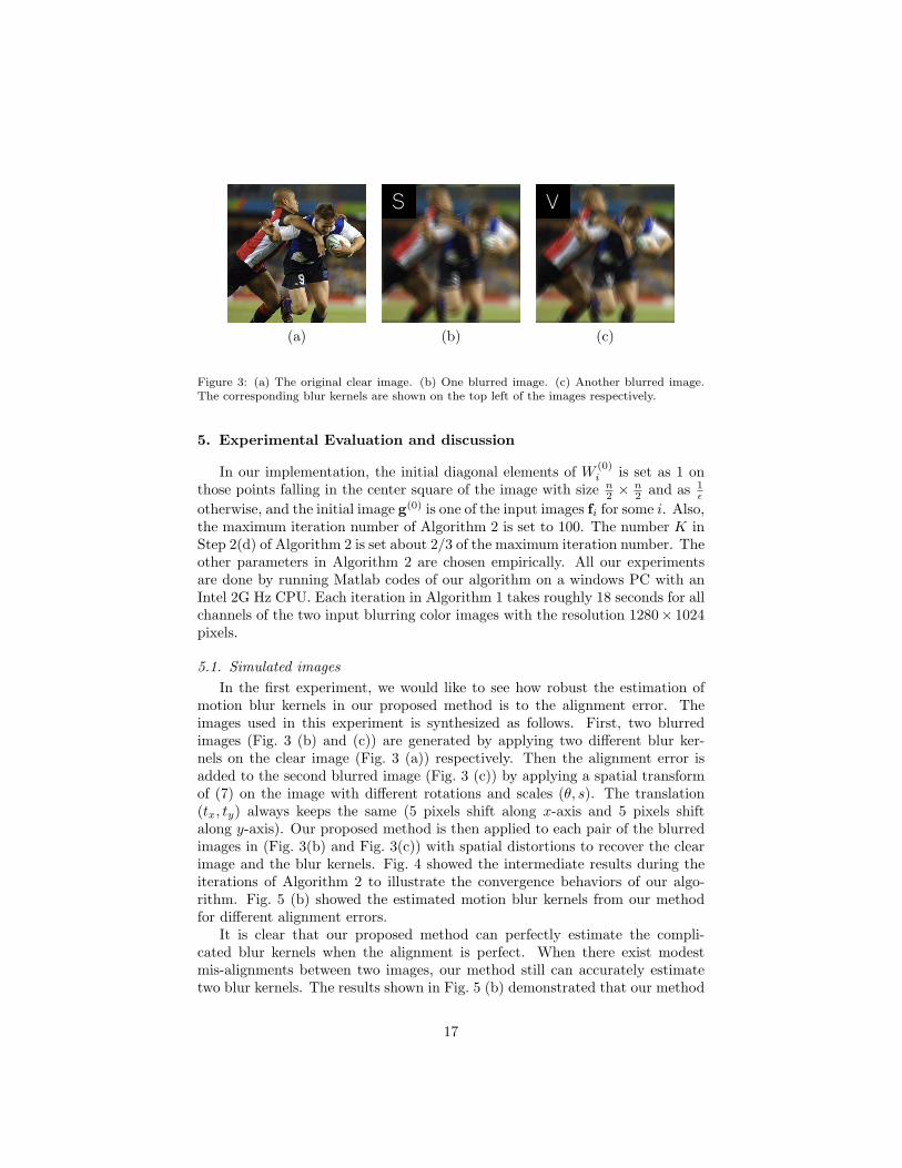
(a) (b) (c)

Figure 3: (a) The original clear image. (b) One blurred image. (c) Another blurred image.The corresponding blur kernels are shown on the top left of the images respectively.

5. Experimental Evaluation and discussion

In our implementation, the initial diagonal elements of W(0)i is set as 1 on

those points falling in the center square of the image with size n2 × n

2 and as 1ǫ

otherwise, and the initial image g(0) is one of the input images fi for some i. Also,the maximum iteration number of Algorithm 2 is set to 100. The number K inStep 2(d) of Algorithm 2 is set about 2/3 of the maximum iteration number. Theother parameters in Algorithm 2 are chosen empirically. All our experimentsare done by running Matlab codes of our algorithm on a windows PC with anIntel 2G Hz CPU. Each iteration in Algorithm 1 takes roughly 18 seconds for allchannels of the two input blurring color images with the resolution 1280× 1024pixels.

5.1. Simulated images

In the first experiment, we would like to see how robust the estimation ofmotion blur kernels in our proposed method is to the alignment error. Theimages used in this experiment is synthesized as follows. First, two blurredimages (Fig. 3 (b) and (c)) are generated by applying two different blur ker-nels on the clear image (Fig. 3 (a)) respectively. Then the alignment error isadded to the second blurred image (Fig. 3 (c)) by applying a spatial transformof (7) on the image with different rotations and scales (θ, s). The translation(tx, ty) always keeps the same (5 pixels shift along x-axis and 5 pixels shiftalong y-axis). Our proposed method is then applied to each pair of the blurredimages in (Fig. 3(b) and Fig. 3(c)) with spatial distortions to recover the clearimage and the blur kernels. Fig. 4 showed the intermediate results during theiterations of Algorithm 2 to illustrate the convergence behaviors of our algo-rithm. Fig. 5 (b) showed the estimated motion blur kernels from our methodfor different alignment errors.

It is clear that our proposed method can perfectly estimate the compli-cated blur kernels when the alignment is perfect. When there exist modestmis-alignments between two images, our method still can accurately estimatetwo blur kernels. The results shown in Fig. 5 (b) demonstrated that our method

17

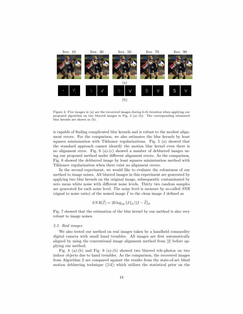
Iter. 10 Iter. 30 Iter. 50 Iter. 70 Iter. 90

(a)

(b)

Figure 4: Five images in (a) are the recovered images during k-th iteration when applying ourproposed algorithm on two blurred images in Fig. 3 (a)–(b). The corresponding estimatedblur kernels are shown in (b).

is capable of finding complicated blur kernels and is robust to the modest align-ment errors. For the comparison, we also estimates the blur kernels by leastsquares minimization with Tikhonov regularizations. Fig. 5 (a) showed thatthe standard approach cannot identify the motion blur kernel even there isno alignment error. Fig. 6 (a)-(c) showed a number of deblurred images us-ing our proposed method under different alignment errors. As the comparison,Fig. 6 showed the deblurred image by least squares minimization method withTikhonov regularization when there exist no alignment errors.

In the second experiment, we would like to evaluate the robustness of ourmethod to image noises. All blurred images in this experiment are generated byapplying two blur kernels on the original image, subsequently contaminated byzero mean white noise with different noise levels. Thirty two random samplesare generated for each noise level. The noise level is measure by so-called SNR(signal to noise ratio) of the noised image I to the clean image I defined as

SNR(I) = 20 log10 ‖I‖2/‖I − I‖2.

Fig. 7 showed that the estimation of the blur kernel by our method is also veryrobust to image noises.

5.2. Real images

We also tested our method on real images taken by a handheld commoditydigital camera with small hand trembles. All images are first automaticallyaligned by using the conventional image alignment method from [2] before ap-plying our method.

Fig. 8 (a)-(b) and Fig. 9 (a)-(b) showed two blurred tele-photos on twoindoor objects due to hand trembles. As the comparison, the recovered imagesfrom Algorithm 2 are compared against the results from the state-of-art blindmotion deblurring technique ([14]) which utilizes the statistical prior on the

18

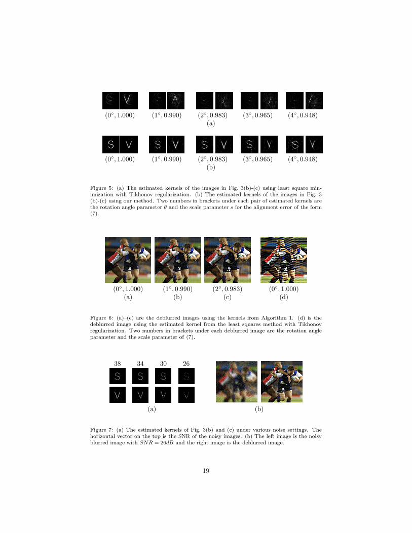
(0◦, 1.000) (1◦, 0.990) (2◦, 0.983) (3◦, 0.965) (4◦, 0.948)(a)

(0◦, 1.000) (1◦, 0.990) (2◦, 0.983) (3◦, 0.965) (4◦, 0.948)(b)

Figure 5: (a) The estimated kernels of the images in Fig. 3(b)-(c) using least square min-imization with Tikhonov regularization. (b) The estimated kernels of the images in Fig. 3(b)-(c) using our method. Two numbers in brackets under each pair of estimated kernels arethe rotation angle parameter θ and the scale parameter s for the alignment error of the form(7).

(0◦, 1.000) (1◦, 0.990) (2◦, 0.983) (0◦, 1.000)(a) (b) (c) (d)

Figure 6: (a)–(c) are the deblurred images using the kernels from Algorithm 1. (d) is thedeblurred image using the estimated kernel from the least squares method with Tikhonovregularization. Two numbers in brackets under each deblurred image are the rotation angleparameter and the scale parameter of (7).

38 34 30 26

(a) (b)

Figure 7: (a) The estimated kernels of Fig. 3(b) and (c) under various noise settings. Thehorizontal vector on the top is the SNR of the noisy images. (b) The left image is the noisyblurred image with SNR = 26dB and the right image is the deblurred image.

19

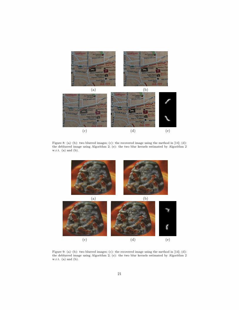
image gradients to derive the motion blur kernel. It is seen that the restoredimage by Algorithm 2 shown in Fig. 8 (d) and Fig. 9 (d) are very clear withlittle artifacts. Obviously, they have much better visual quality than the imagesrestored by the method from [14] which are shown in Fig. 8 (c) and Fig. 9 (c).

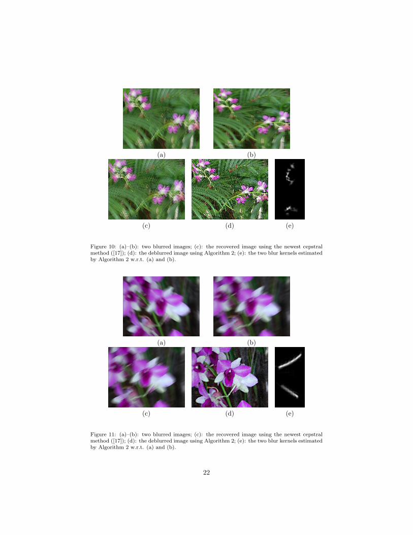
We also tested our method on out-door scenes. The blurred images on out-door scenes usually tend to be more difficult to deblur as there are multiple layersof blurring due to more complicated 3D structures, e.g., out-of-focus blurringand moving objects. Also, the complex image structure of typical outdoor scenesmakes the deblurring process more challenging. Fig. 8 (a)-(b) and Fig. 9 (a)-(b) showed two blurred image pairs on two out-door scenes. We comparedthe results from Algorithm 2 to the results from more traditional cepstrum-based approach ([17]). Obviously, the results from Algorithm 2 are much betterthan those using the method from [17]. However, the restored images shownin Fig. 10 (d) and Fig. 11 (d) are less impressive than the previous results ofin-door images. One reason is that the framelet coefficients of images with richtextures are not as sparse as those of images with less textures, which resultsin less robustness of our deblurring algorithm to image noises. Also, there aremore noticable artifacts in Fig. 10 (d) than in Fig. 11 (d). The reason could bethat the actual blurring for the case of Fig. 10 is the mixture of multiple blurringprocess and our model only focuses on the motion blurring. One evidence is thatthe estimated blur kernels shown in Fig. 10 (e) are not in the form of typicalmotion-blur kernels. Another possible reason could be that the blurring kernelof Fig. 10 is not spatial invariant due to the wind blowing the leaves during thecamera exposure. This can be seen from the fact that the artifacts in Fig. 10 (e)have different directions for different leaves.

5.3. Conclusion and future work

Using multiple images not only improves the condition on deconvolutionprocess, but also provides more information to help the identification of com-plicated motion blurring. However, the benefits of using multiple images cannot be easily materialized by the standard approaches as the unavoidable imagealignment errors could eliminate all the advantages of using multiple images.In this paper, we proposed an approach to recover the high-quality clear im-age by using multiple images to accurately identify motion blur kernels. Byusing the sparsity constraints on the images and on the blur kernels in suitabledomains, the proposed approach is robust to the image formation noise andmore importantly robust to the image alignment errors. Furthermore, basedon the linearized Bregman iteration technique, we developed a fast approxi-mate algorithm to find a good approximate solution to the resulting large-scaleminimization problem very efficiently.

Our proposed method does not require a prior parametric model on the mo-tion blur kernel, and does not require accurate image alignment among frames.These two properties greatly extend the applicability of motion deblurring ongeneral video sequences in practice. In future, we would like to investigate thelocalization of our algorithm on spatial-variant motion blurring such as deblur-ring fast-moving objects in the image. Also, we are interested in investigating

20

(a) (b)

(c) (d) (e)

Figure 8: (a)–(b): two blurred images; (c): the recovered image using the method in [14]; (d):the deblurred image using Algorithm 2; (e): the two blur kernels estimated by Algorithm 2w.r.t. (a) and (b).

(a) (b)

(c) (d) (e)

Figure 9: (a)–(b): two blurred images; (c): the recovered image using the method in [14]; (d):the deblurred image using Algorithm 2; (e): the two blur kernels estimated by Algorithm 2w.r.t. (a) and (b).

21

(a) (b)

(c) (d) (e)

Figure 10: (a)–(b): two blurred images; (c): the recovered image using the newest cepstralmethod ([17]); (d): the deblurred image using Algorithm 2; (e): the two blur kernels estimatedby Algorithm 2 w.r.t. (a) and (b).

(a) (b)

(c) (d) (e)

Figure 11: (a)–(b): two blurred images; (c): the recovered image using the newest cepstralmethod ([17]); (d): the deblurred image using Algorithm 2; (e): the two blur kernels estimatedby Algorithm 2 w.r.t. (a) and (b).

22

how to incorporate the image alignment of blurred image into the proposedminimization to achieve even better performance.

References

[1] H. C. Andrews, B. R. Hunt, Digital image restoration, Prentice-Hall, En-glewood Cliffs, NJ, 1977.

[2] J. Bergen, P. Anandan, K. Hanna, R. Hingorani, Hierarchical model-basedmotion estimation, in: ECCV, 1992.

[3] M. Ben-Ezra, S. K. Nayar, Motion-based motion deblurring, IEEE Trans.Pattern Aanalysis and Machine Intelligence 26 (6) (2004) 689–698.

[4] J.-F. Cai, S. Osher, Z. Shen, Linearized Bregman iterations for compressedsensing, Mathematics of Computation 78 (2009) 1515–1536.

[5] J.-F. Cai, S. Osher, Z. Shen, Linearized Bregman iterations for frame-basedimage deblurring, SIAM J. Imaging Sci. 2 (1) (2009) 226–252.

[6] J.-F. Cai, S. Osher, Z. Shen, Convergence of the linearized Bregman it-eration for ℓ1-norm minimization, Mathematics of Computation 78 (2009)2127–2136.

[7] A. Chai, Z. Shen, Deconvlolution: A wavelet frame approach, Numer.Math. 106 (2007) 529–587.

[8] T. F. Chan, J. Shen, Image processing and analysis, Variational, PDE,wavelet, and stochastic methods, Society for Industrial and Applied Math-ematics (SIAM), Philadelphia, PA, 2005.

[9] T. F. Chan, C. K. Wong, Total variation blind deconvolution, IEEE Tran.Image Processing 7 (3) (1998) 370–375.

[10] M. M. Chang, A. M. Tekalp, A. T. Erdem, Blur identification using thebispectrum, IEEE transactions on signal processing 39 (1991) 2323–2325.

[11] J. Darbon, S. Osher, Fast discrete optimization for sparse approximationsand deconvolutions, in: preprint, 2007.

[12] I. Daubechies, B. Han, A. Ron, Z. Shen, Framelets: MRA-based construc-tions of wavelet frames, Appl. Comput. Harmon. Anal. 14 (2003) 1–46.

[13] D. C. Dobson, F. Santosa, Recovery of blocky images from noisy andblurred data, SIAM J. Appl. Math. 56 (1996) 1181–1198.

[14] R. Fergus, B. Singh, A. Hertzmann, S. T. Roweis, W. T. Freeman, Re-moving camera shake from a single photograph, SIGGRAPH, 25 (2006)783–794.

23

[15] T. Goldstein, S. Osher, The split Bregman algorithm for l1 regularizedproblems, UCLA CAM Reports (08-29).

[16] L. He, A. Marquina, S. J. Osher, Blind deconvolution using TV regular-ization and Bregman iteration, Int. J. Imaging Syst. Technol. 15 (2005)74–83.

[17] H. Ji, C. Q. Liu, Motion blur identification from image gradients, in: Pro-ceeding of IEEE Computer Society conference on computer vision and pat-tern recognition, (2008) 1–8.

[18] Y. Lou, X. Zhang, S. Osher, A. Bertozzi, Image recovery via nonlocaloperators, UCLA CAM Reports (08-35).

[19] Y. Lu, J. Sun, Q. L., H. Shum, Blurred/non-blurred image alignment usingkernel sparseness prior, IEEE Int. Conf. on Computer Vision (2007).

[20] A. Marquina, Inverse scale space methods for blind deconvolution, UCLACAM Reports (06-36).

[21] C. Mayntz, T. Aach, Blur identification using a spectral inertia tensor andspectral zeros, IEEE transacions on image processing 2 (1999) 885–559.

[22] M. K. Ng, R. H. Chan, W. Tang, A fast algorithm for deblurring modelswith neumann boundary condition, SIAM J. Sci. Comput. 21 (3) (2000)851–866.

[23] M. Nikolova, Local strong homogeneity of a regularized estimator, SIAMJ. Appl. Math. 61 (2000) 633–658.

[24] S. Osher, M. Burger, D. Goldfarb, J. Xu, W. Yin, An iterative regulariza-tion method for total variation-based image restoration, Multiscale Model.Simul. 4 (2005) 460–489.

[25] S. Osher, Y. Mao, B. Dong, W. Yin, Fast linearized Bregman iteration forcompressed sensing and sparse denoising, UCLA CAM Reprots (08-37).

[26] A. Rav-Acha, S. Peleg, Two motion blurred images are better than one,Pattern Recognition Letters 26 (2005) 311–317.

[27] R. Raskar, J. Tubmlin, A. Mohan, A. Agrawal, Y. Li, Computational pho-tography, EUROGRAPHICS (2006).

[28] R. Raskar, A. Agrawal, J. Tumblin, Coded exposure photography: Motiondeblurring via fluttered shutter, SIGGRAPH 25 (2006) 795–804.

[29] I. M. Rekleitis, Steerable filters and cepstral analysis for optical flow cal-culation from a single blurred image, Vision Interface 1 (1996) 159–166.

[30] A. Ron, Z. Shen, Affine system in l2(rd): the analysis of the analysis oper-

ator, Journal of Functional Analysis 148 (1997) 408–447.

24

[31] J. Xu, S. J. Osher, Iterative regularization and nonlinear inverse scale spaceapplied to wavelet-based denoising, IEEE Trans. Image Process. 16 (2007)534–544.

[32] W. Yin, S. Osher, D. Goldfarb, J. Darbon, Bregman iterative algorithms forℓ1-minimization with applications to compressed sensing, SIAM J. ImagingSci. 1 (2008) 143–168.

[33] Y. Yitzhaky, I. Mor, A. Lantzman, N. S. Kopeika, Direct method forrestoration of motion-blurred images, J. Opt. Soc. Am. 15 (6) (1998) 1512–1519.

[34] B. Zitova, J. Flusser, Image registration methods: a survey, Image andVision Computing 21 (11) (2003) 977–1000.

25