BLIND ESTIMATION WITHOUT PRIORS:

PERFORMANCE, CONVERGENCE, AND EFFICIENT

IMPLEMENTATION

A Dissertation

Presented to the Faculty of the Graduate School

of Cornell University

in Partial Fulfillment of the Requirements for the Degree of

Doctor of Philosophy

by

Philip Schniter

May 2000

c© Philip Schniter 2000

ALL RIGHTS RESERVED

BLIND ESTIMATION WITHOUT PRIORS: PERFORMANCE,

CONVERGENCE, AND EFFICIENT IMPLEMENTATION

Philip Schniter, Ph.D.

Cornell University 2000

We address the problem of estimating a distorted signal in the presence of noise

in the case that very little prior knowledge is available regarding the nature of the

signal, the distortion, or the noise. More specifically, we assume that the distorting

system is linear but otherwise unknown, that the signal is drawn from a sequence of

independent and identically distributed random variables of unknown distribution,

and that the noise is independent of the signal but also has unknown distribution.

We refer to this problem as “blind estimation without priors,” where the term

“blind” captures the notion that signal estimates are obtained blindly with regard

to knowledge of the distortion and interference.

Since its origins nearly half a century ago, there has evolved a large body of

theoretical and practical knowledge regarding the blind estimation problem. Even

so, very fundamental questions still remain. For example: (i) How good are blind

estimates compared to their non-blind counterparts? (ii) When do we know that

a blind estimation algorithm will return estimates of the desired signal versus a

component of the interference? Though both of these questions have long histories

within the research community, existing results have been either approximate and/or

limited to special cases that leave out many problems of practical interest.

This dissertation presents answers to the questions above for the well-known

Shalvi-Weinstein (SW) and constant modulus (CM) approaches to blind linear es-

timation. All results are derived in a general setting: vector-valued infinite im-

pulse response channels, constrained vector-valued auto-regressive moving-average

estimators, and near-arbitrary forms of signal and interference. First, we derive

concise expressions tightly upper bounding the mean-squared error (MSE) of SW

and CM-minimizing estimates which are principally a function of the optimum MSE

achievable in the same setting. Second, we derive similar bounds for the average

squared parameter error in CM-based blind channel identification. Third, we present

sufficient conditions for gradient-descent (GD) initializations that guarantee conver-

gence to CM-minimizing estimates of the desired user. These conditions principally

involve the signal-to-interference ratio of the initial estimates. Finally, we propose

a novel approach to CM-GD implementation that greatly reduces the implemen-

tation complexity of the standard CM-GD algorithm while still retaining its mean

behavior.

Biographical Sketch

Philip Schniter was born in Evanston IL in the summer of 1970. He received the

B.S. and M.S. degrees in electrical and computer engineering from the University of

Illinois at Urbana-Champaign in 1992 and 1993, respectively. From 1993 to 1996 he

was employed by Tektronix Inc. in Beaverton OR as a Systems Engineer. There he

worked on signal processing aspects of video and communications instrumentation

design, including algorithms, software, and hardware architectures.

Since 1996 he has been working toward the Ph.D. degree in electrical engineer-

ing at Cornell University, Ithaca, NY, where he received the 1998 Schlumberger

Fellowship and the 1998-99 Intel Foundation Fellowship. His research interests are

in the areas of signal processing and data communication, with special emphasis on

adaptive systems.

iii

To my parents, Jorg and Martha Schniter, for their love and support,

and

in fond memory of David F. C. Simmonds.

iv

Acknowledgements

I’ve had a phenomenal time during my four years in Ithaca, and I attribute my good

fortune to the wonderful people I’ve come to know through my Cornell experience.

First and foremost, I would like to thank my supervisor Prof. C. Richard Johnson,

Jr., for his generosity and support over the years. I will always remember Rick as

“the advisor who made everything possible.” His friendliness, wisdom, spontaneity,

and sense of adventure make him unique in the academic community. Many thanks

also go to my committee members, Profs. Lang Tong and Venu Veeravalli; they have

provided me with invaluable guidance, encouragement, and inspiration throughout

the last four years. These acknowledgements would be far from complete without

heartfelt thanks to Profs. Doug Jones and Mike Orchard for their sage advice before

and during my studies at Cornell, as well as Prof. Vince Poor and Dr. John Treichler

for their genuine friendliness, support, and interest in my work.

Next, I want to thank the colleagues of mine who made Rhodes Hall a thoroughly

entertaining, if not always productive, place to work. In order of appearance... Tom

“Shotgun” Endres: seeing your John Deere hat during my first campus visit, I

knew I belonged in the research group; Raul “Buddy Boy” Casas: a more friendly,

helpful, spontaneous, and entertaining officemate cannot be imagined (and I still

owe you a super-soaking); Knox Carey: your friendship and Linux wizardry were

v

huge helps during my first year at Cornell—long live the pedal steel; Rick “Vanilla”

Brown: whether it be Linux, latex, math, or the job hunt, you’ve been generous

with your help and plentiful with your (base) humor—its been a fun ride; Won-

zoo “The Dragon” Chung: your appetite for knowledge, cross-cultural understand-

ing, and large quantities of (jumping!) hot food has earned my deepest respect;

Jaiganesh “Jai” Balakrishnan: your keen insights and kind ways are have been

much appreciated; Andy Klein and Don Anair: ahhh, fond memories of rides in the

van, walks on the beach, and all the good clean fun we’ve had; Azzedine Touzni:

from our first meeting, your open-mindedness, generosity, and cultured European

ways have always impressed me—it was great having you in Ithaca; Prof. Bill “6σ”

“signum” Sethares: the late-night discussions, plastic-sax jams, and spaghetti din-

ners are fondly remembered—thanks for your sage advice and willingness to lend

an ear anytime. Thanks also go to the visiting researchers Sangarapillai “Lambo”

Lambotharan, Prof. Michael Green, and Jim Behm, for their assistance and com-

panionship.

Indispensable to the completion of my degree were the many hours of ultimate

frisbee at Helen-Newman, Belle-Sherman, and Cass Park; summer swimming at the

6-mile Creek reservoir and winter swimming at Teagle; hiking and cross-country

skiing in the local hills and forests; playing/hearing live music at the local clubs

and festivals; and raging at the countless (yet always memorable) parties. These

activities wouldn’t have been the same if it wasn’t for my good friends Kather-

ine Alaimo, Marisa Alcorta, Kristin Arend, Corien Bakermans, Ami Ben-Yaacov,

Francis Chan, Peter Choi, Diane Decker, Peter Dees, Maile and Todd Deppe, Jesse

Ernst, Thamora Fishel, Jen Fiskin, Anne Gallagher, Pete Hedlund, Ruth Hufbauer,

Bill Huston, Laci, Loden, Tawainga Katsvairo, Frank Adelstein, Ketch and Critter,

vi

Brady Moss, Matt Nemeth, Eric Odell, Kevin Pilz, Deepak Ramani, Mary Reeves,

Art Rodgers, Art Schaub, Martin Schlaepfer, Sunjya & Lia Schweig, Kurt Smemo,

Bob Turner, Mace Vaughan, Dave Walker, Rob Young, and Brooke Zanatell. Spe-

cial mention is given to the following dear friends, for all that they have added to

my life over the last four years: Tony Anderson, Ruby Beil, Ryan Budney, Heather

Clark, and Beth Conrey. Finally, saving the best for last, I want to thank the sweet

and wonderful Caroline Simmonds for all the sunshine she’s brought to my last year

and a half in Ithaca.

My studies were funded by the National Science Foundation (under grants MIP-

9509011, MIP-9528363, and ECS-9811297), Applied Signal Technology Inc., the

Intel Foundation, and the Schlumberger Foundation.

vii

Table of Contents

1 Introduction 1

2 Background 102.1 Introduction to Blind Estimation without Priors . . . . . . . . . . . . 10

2.1.1 A Simple Model . . . . . . . . . . . . . . . . . . . . . . . . . . 112.1.2 The Problem with Classical Techniques . . . . . . . . . . . . . 122.1.3 Ambiguities Inherent to BEWP . . . . . . . . . . . . . . . . . 142.1.4 On Linear Combinations of I.I.D. Random Variables . . . . . 162.1.5 Implications for Blind Linear Estimation . . . . . . . . . . . . 182.1.6 Examples of Admissible Criteria for Linear BEWP . . . . . . 222.1.7 Summary and Unanswered Questions . . . . . . . . . . . . . . 24

2.2 A General Linear Model . . . . . . . . . . . . . . . . . . . . . . . . . 252.3 Mean-Squared Error Criteria . . . . . . . . . . . . . . . . . . . . . . . 31

2.3.1 The Mean-Squared Error Criterion . . . . . . . . . . . . . . . 322.3.2 Unbiased Mean-Squared Error . . . . . . . . . . . . . . . . . . 322.3.3 Signal to Interference-Plus-Noise Ratio . . . . . . . . . . . . . 33

2.4 The Shalvi-Weinstein Criterion . . . . . . . . . . . . . . . . . . . . . 332.5 The Constant Modulus Criterion . . . . . . . . . . . . . . . . . . . . 352.A Derivation of MMSE Estimators . . . . . . . . . . . . . . . . . . . . . 38

3 Bounds for the MSE performance of SW Estimators 403.1 Introduction . . . . . . . . . . . . . . . . . . . . . . . . . . . . . . . . 403.2 SW Performance under General Additive Interference . . . . . . . . . 42

3.2.1 The SW-UMSE Bounding Strategy . . . . . . . . . . . . . . . 423.2.2 The SW-UMSE Bounds . . . . . . . . . . . . . . . . . . . . . 473.2.3 Comments on the SW-UMSE Bounds . . . . . . . . . . . . . . 50

3.3 Numerical Examples . . . . . . . . . . . . . . . . . . . . . . . . . . . 533.4 Conclusions . . . . . . . . . . . . . . . . . . . . . . . . . . . . . . . . 573.A Derivation Details for SW-UMSE Bounds . . . . . . . . . . . . . . . . 59

3.A.1 Proof of Theorem 3.1 . . . . . . . . . . . . . . . . . . . . . . . 593.A.2 Proof of Theorem 3.2 . . . . . . . . . . . . . . . . . . . . . . . 653.A.3 Proof of Theorem 3.3 . . . . . . . . . . . . . . . . . . . . . . . 67

viii

4 Bounds for the MSE performance of CM Estimators 704.1 Introduction . . . . . . . . . . . . . . . . . . . . . . . . . . . . . . . . 704.2 CM Performance under General Additive Interference . . . . . . . . . 72

4.2.1 The CM-UMSE Bounding Strategy . . . . . . . . . . . . . . . 744.2.2 Derivation of the CM-UMSE Bounds . . . . . . . . . . . . . . 774.2.3 Comments on the CM-UMSE Bounds . . . . . . . . . . . . . . 81

4.3 Numerical Examples . . . . . . . . . . . . . . . . . . . . . . . . . . . 834.3.1 Performance versus Estimator Length for Fixed Channel . . . 844.3.2 Performance versus AWGN for Fixed Channel . . . . . . . . . 854.3.3 Performance with Random Channels . . . . . . . . . . . . . . 86

4.4 Conclusions . . . . . . . . . . . . . . . . . . . . . . . . . . . . . . . . 874.A Derivation Details for CM-UMSE Bounds . . . . . . . . . . . . . . . 92

4.A.1 Proof of Lemma 4.1 . . . . . . . . . . . . . . . . . . . . . . . . 924.A.2 Proof of Lemma 4.2 . . . . . . . . . . . . . . . . . . . . . . . . 934.A.3 Proof of Lemma 4.3 . . . . . . . . . . . . . . . . . . . . . . . . 934.A.4 Proof of Theorem 4.1 . . . . . . . . . . . . . . . . . . . . . . . 964.A.5 Proof of Theorem 4.2 . . . . . . . . . . . . . . . . . . . . . . . 994.A.6 Proof of Theorem 4.3 . . . . . . . . . . . . . . . . . . . . . . . 102

5 Sufficient Conditions for the Local Convergence of CM Algorithms1045.1 Introduction . . . . . . . . . . . . . . . . . . . . . . . . . . . . . . . . 1045.2 Sufficient Conditions for Local Convergence of CM-GD . . . . . . . . 107

5.2.1 The Main Idea . . . . . . . . . . . . . . . . . . . . . . . . . . 1075.2.2 Derivation of Sufficient Conditions . . . . . . . . . . . . . . . 109

5.3 Implications for CM Initialization Schemes . . . . . . . . . . . . . . . 1125.3.1 The “Single-Spike” Initialization . . . . . . . . . . . . . . . . . 1135.3.2 Initialization Using Partial Information . . . . . . . . . . . . . 114

5.4 Numerical Examples . . . . . . . . . . . . . . . . . . . . . . . . . . . 1165.5 Conclusions . . . . . . . . . . . . . . . . . . . . . . . . . . . . . . . . 1195.A Derivation Details for Local Convergence Conditions . . . . . . . . . 122

5.A.1 Proof of Lemma 5.1 . . . . . . . . . . . . . . . . . . . . . . . . 1225.A.2 Proof of Theorem 5.1 . . . . . . . . . . . . . . . . . . . . . . . 1265.A.3 Proof of Theorem 5.2 . . . . . . . . . . . . . . . . . . . . . . . 1275.A.4 Proof of Theorem 5.3 . . . . . . . . . . . . . . . . . . . . . . . 128

6 Performance Bounds for CM-Based Channel Identification 1336.1 Introduction . . . . . . . . . . . . . . . . . . . . . . . . . . . . . . . . 1336.2 Blind Identification – Performance Bounds . . . . . . . . . . . . . . . 1366.3 Blind Identification – Issues in Practical Implementation . . . . . . . 138

6.3.1 ASPE with Finite-Data Correlation Approximation . . . . . . 1386.3.2 Stochastic Gradient Estimation of CM Equalizer . . . . . . . . 1396.3.3 Effect of Residual Carrier Offset . . . . . . . . . . . . . . . . . 141

6.4 Numerical Examples . . . . . . . . . . . . . . . . . . . . . . . . . . . 1436.5 Conclusions . . . . . . . . . . . . . . . . . . . . . . . . . . . . . . . . 144

ix

6.A Derivation Details for Channel Identification Bounds . . . . . . . . . 1496.A.1 Proof of Theorem 6.1 . . . . . . . . . . . . . . . . . . . . . . . 1496.A.2 Proof of Lemma 6.1 . . . . . . . . . . . . . . . . . . . . . . . . 151

7 Dithered Signed Error CMA 1547.1 Introduction . . . . . . . . . . . . . . . . . . . . . . . . . . . . . . . . 1547.2 Computationally Efficient CMA . . . . . . . . . . . . . . . . . . . . . 156

7.2.1 Signed-Error CMA . . . . . . . . . . . . . . . . . . . . . . . . 1567.2.2 Dithered Signed-Error CMA . . . . . . . . . . . . . . . . . . . 158

7.3 The Fundamental Properties of DSE-CMA . . . . . . . . . . . . . . . 1607.3.1 Quantization Noise Model of DSE-CMA . . . . . . . . . . . . 1607.3.2 DSE-CMA Transient Behavior . . . . . . . . . . . . . . . . . . 1617.3.3 DSE-CMA Cost Surface . . . . . . . . . . . . . . . . . . . . . 1657.3.4 DSE-CMA Steady-State Behavior . . . . . . . . . . . . . . . . 170

7.4 DSE-CMA Design Guidelines . . . . . . . . . . . . . . . . . . . . . . 1737.4.1 Selection of Dispersion Constant γ . . . . . . . . . . . . . . . 1737.4.2 Selection of Dither Amplitude α . . . . . . . . . . . . . . . . . 1737.4.3 Selection of Step-Size µ . . . . . . . . . . . . . . . . . . . . . . 1747.4.4 Initialization of DSE-CMA . . . . . . . . . . . . . . . . . . . . 175

7.5 Simulation Results . . . . . . . . . . . . . . . . . . . . . . . . . . . . 1767.5.1 Excess MSE for FCR H . . . . . . . . . . . . . . . . . . . . . 1767.5.2 Average Transient Behavior . . . . . . . . . . . . . . . . . . . 1777.5.3 Comparison with Update-Decimated CMA . . . . . . . . . . . 180

7.6 Conclusions . . . . . . . . . . . . . . . . . . . . . . . . . . . . . . . . 1817.A Properties of Non-Subtractively Dithered Quantizers . . . . . . . . . 1847.B Derivation of F (n+1) . . . . . . . . . . . . . . . . . . . . . . . . . . 1857.C Derivation of Jex . . . . . . . . . . . . . . . . . . . . . . . . . . . . . 188

8 Concluding Remarks 1908.1 Summary of Original Work . . . . . . . . . . . . . . . . . . . . . . . . 1918.2 Possible Future Work . . . . . . . . . . . . . . . . . . . . . . . . . . . 193

Bibliography 195

x

List of Tables

1.1 Examples of the blind estimation problem. . . . . . . . . . . . . . . . 3

4.1 Zeng et al.s’ CM-UMSE bounding algorithm. . . . . . . . . . . . . . 73

5.1 Single-spike kurtoses for SPIB microwave channel models. . . . . . . 114

7.1 Critical values of α for M-PAM. . . . . . . . . . . . . . . . . . . . . 1667.2 Steady-state MSE relative performance factor. . . . . . . . . . . . . 1757.3 Jex deviation from predicted level for various SPIB channels. . . . . . 176

8.1 Correspondence between dissertation chapters and journal submis-sions/publications. . . . . . . . . . . . . . . . . . . . . . . . . . . . . 193

xi

List of Figures

1.1 Dissertation map. . . . . . . . . . . . . . . . . . . . . . . . . . . . . 8

2.1 Stationary SISO observation model. . . . . . . . . . . . . . . . . . . 112.2 Blind linear estimation. . . . . . . . . . . . . . . . . . . . . . . . . . 192.3 MIMO linear system model with K sources of interference. . . . . . . 26

3.1 Illustration of Q(0)ν . . . . . . . . . . . . . . . . . . . . . . . . . . . . . 45

3.2 Illustration of SW-UMSE bounding technique. . . . . . . . . . . . . 473.3 Upper bound on SW-UMSE and extra SW-UMSE. . . . . . . . . . . 513.4 Bounds on SW-UMSE for sub-Gaussian signal and random H. . . . 543.5 Bounds on SW-UMSE for super-Gaussian signal and random H. . . 553.6 Bounds on SW-UMSE for near-Gaussian signal and random H. . . . 563.7 Bounds on SW-UMSE for impulsive interference and random H. . . 573.8 Example of P2(x) and disjoint Qsw(qr,ν). . . . . . . . . . . . . . . . . 613.9 Example of P2(x), Qsw(qr,ν), and bounding radius. . . . . . . . . . . 623.10 Illustration of local minima existence arguments. . . . . . . . . . . . 64

4.1 Illustration of CM-UMSE upper-bounding technique. . . . . . . . . . 764.2 Upper bound on CM-UMSE and extra CM-UMSE. . . . . . . . . . . 814.3 Bounds on CM-UMSE versus estimator length. . . . . . . . . . . . . 854.4 Bounds on CM-UMSE versus SNR of AWGN. . . . . . . . . . . . . . 864.5 Bounds on CM-UMSE for random H. . . . . . . . . . . . . . . . . . 884.6 Bounds on CM-UMSE for near-Gaussian signal & random H. . . . . 894.7 Bounds on CM-UMSE for super-Gaussian interference & random H. 90

5.1 Illustration of sufficient SINR derivation technique. . . . . . . . . . . 1105.2 CM-GD trajectories showing convergence behavior. . . . . . . . . . . 1185.3 Estimated probability of convergence to desired source/delay. . . . . 120

6.1 Linear system model with K sources of interference. . . . . . . . . . 1346.2 Blind channel identification using CM estimates {yn} ≈ {s(0)

n−ν}. . . . 1346.3 Gooch-Harp method of blind channel identification. . . . . . . . . . . 1356.4 Linear system model with residual carrier offset . . . . . . . . . . . . 1426.5 Mean-squared parameter error versus SNR of AWGN. . . . . . . . . 1456.6 Mean-squared parameter error versus symbol estimator length. . . . 146

xii

6.7 Estimation error for SPIB microwave channel #3. . . . . . . . . . . . 1476.8 Estimation error for SPIB microwave channel #2. . . . . . . . . . . . 148

7.1 CMA, SE-CMA, and DSE-CMA error functions. . . . . . . . . . . . 1577.2 SE-CMA trajectories superimposed on Jc cost contours. . . . . . . . 1587.3 Quantization noise model (right) of the dithered quantizer (left). . . 1607.4 CMA error function and critical α for 4-PAM and 16-PAM sources. . 1667.5 Superimposed DSE-CMA and CMA cost contours in equalizer space. 1687.6 Trajectories of DSE-CMA overlaid on those of CMA. . . . . . . . . . 1697.7 Comparison of DSE-CMA and CMA averaged trajectories. . . . . . . 1787.8 Averaged trajectories superimposed on CM cost contours. . . . . . . 1797.9 Comparison of DSE-CMA and UD-CMA averaged trajectories. . . . 181

xiii

List of Abbreviations

Abbreviation Journal Name

ASSPM IEEE Acoustics Speech and Signal Processing MagazineATT AT&T Technical JournalBSTJ Bell System Technical JournalGEO GeoexplorationGP Geophysical ProspectingIJACSP Internat. Journal of Adaptive Control & Signal ProcessingOE Optical EngineeringETS Educational Testing Service Research BulletinPROC Proceedings of the IEEEPSY PsychometrikaSEP Stanford Exploration ProjectSP Signal ProcessingSPL IEEE Signal Processing LettersSPM IEEE Signal Processing MagazineTASSP IEEE Trans. on Acoustics, Speech, and Signal ProcessingTCOM IEEE Trans. on CommunicationsTIT IEEE Trans. on Information TheoryTSP IEEE Trans. on Signal Processing

Abbreviation Conference Name

ALL Allerton Conf. on Communication, Control, and ComputingASIL Asilomar Conf. on Signals, Systems and ComputersCISS Conf. on Information Science and SystemsGLOBE IEEE Global Telecommunications Conf.ICASSP IEEE Internat. Conf. on Acoustics, Speech, and Signal

ProcessingICC IEEE Intern. Conf. on CommunicationNNSP IEEE Workshop on Neural Networks for Signal ProcessingSPAWC IEEE Internat. Workshop on Signal Processing Advances

in Wireless CommunicationsSPIE The Internat. Society for Optical EngineeringWCNC IEEE Wireless Communication and Networking Conf.WICASS Internat. Workshop on Independent Component Analysis

and Signal Separation

xiv

Abbreviation Meaning

ARMA Auto-Regressive Moving-AverageASPE Average-Squared Parameter ErrorAWGN Additive White Gaussian NoiseBEWP Blind Estimation Without PriorsBIBO Bounded-Input Bounded-OutputBMSE Bayesian Mean-Squared ErrorBPSK Binary Phase Shift KeyingBSE Baud-Spaced EqualizerCDMA Code Division Multiple AccessCM Constant ModulusCMA Constant Modulus AlgorithmDSE Dithered Signed ErrorEMSE Excess Mean-Squared ErrorFCR Full Column RankFIR Finite Impulse ResponseFSE Fractionally-Spaced EqualizerGD Gradient DescentHDTV High Definition TelevisionHOS Higher-Order Statisticsi.i.d. Independent and Identically DistributedIIR Infinite Impulse ResponseISI Inter-Symbol InterferenceLMS Least Mean SquareLTI Linear Time-InvariantMAI Multi-Access InterferenceMAP Maximum A PosterioriMIMO Multiple Input Multiple OutputML Maximum LikelihoodMMSE Minimum Mean-Squared ErrorMSE Mean-Squared ErrorPAM Pulse Amplitude ModulationPBLE Perfect Blind Linear EstimationPSD Positive Semi-DefiniteROC Region of ConvergenceQAM Quadrature Amplitude ModulationQPSK Quadrature Phase Shift KeyingSE Signed ErrorSER Symbol Error RateSINR Signal to Interference-Plus-Noise RatioSISO Single Input Single OutputSNR Signal to Noise RatioSOS Second-Order StatisticsSPIB Signal Processing Information Base1

SW Shalvi-Weinstein

1See http://spib.rice.edu/spib/microwave.html.

xv

Abbreviation Meaning

UD Update DecimatedUMSE Conditionally-Unbiased Mean-Squared ErrorZF Zero Forcing

xvi

List of Symbols

Notation DefinitionE{·} Expectation(·)t Transposition(·)∗ Conjugation(·)H Hermitian transpose (i.e., conjugate transpose)(·)† Moore-Penrose pseudo-inversetr(·) Trace operator for square matricesrow(·) Row span of a matrixcol(·) Column span of a matrixdiag(·) Extraction of diagonal matrix elementsλmin(·) Minimum eigenvalueλmax(·) Maximum eigenvalueσ(·) Singular value`p The space of sequences {xn} such that

∑

n |xn|p <∞‖x‖p `p norm: p

√∑

n |xn|p‖x‖

ANorm defined by

√xHAx for positive definite Hermitian A

I Identity matrixei Column vector with 1 at the ith entry (i ≥ 0) and zeros elsewhereRp The field of p-dimensional real-valued vectorsCp The field of p-dimensional complex-valued vectorsRe(·) Extraction of real-valued componentIm(·) Extraction of imaginary-valued componentsgn(·) Real-valued sign operator: sgn(x) = 1 for x ≥ 0, else sgn(x) = −1csgn(·) Complex-valued sign operator: csgn(x) := sgn(Rex) + j sgn(Im x)∇f Gradient with respect to f : ∇f := ∂

∂fr+ j ∂

∂fifor fr = Re f , fi = Im f

bndr(·) Boundary of a setintr(·) Interior of a set

xvii

Chapter 1

Introduction

Estimation of a distorted signal in noise is a classic problem that finds important

application in areas including, but not limited to,

• data communication [Gitlin Book 92], [Lee Book 94], [Proakis Book 95],

• radar signal processing [Haykin Book 92],

• sensor array processing [Compton Book 88], [VanVeen ASSPM 88],

• geophysical exploration [Mendel Book 83], [Robinson Book 86],

• speech processing [Deller Book 93],

• image analysis [Jain Book 89],

• biomedicine [Akay Book 96], and

• control systems [Anderson Book 89], [Doyle Book 91].

A mathematical model describing this problem is

r = H(s) + w. (1.1)

Here the observed vector r is modeled as a signal vector s distorted by function

H(·) and corrupted by additive noise w.

1

2

Different estimation problems can be characterized by the assumptions placed

on H(·), s, and w. Though central limit theorem arguments are commonly used

to justify a Gaussian noise model for w, the assumptions on H(·) and s can differ

significantly from one application to the next. For example, is H(·) completely

known? If not, is it because H(·) is inherently random? Assuming random H(·),

do we know its distribution? If not, can variabilities in the distribution or structure

of H(·) be described with a small set of parameters? Similar questions can be

asked about the signal s or about the noise w when the Gaussian assumption is not

adequate. In general, the introduction of accurate prior assumptions about H(·), s,

and w, allows the design of estimators with increased performance (though perhaps

more complicated implementation). If prior assumptions are inaccurate, however,

estimator performance can suffer significantly.

There exist many applications of estimation theory where prior knowledge is

lacking and accurate assumptions are hard to come by. In this dissertation we focus

on a relatively extreme lack of knowledge. Specifically, we assume that

1. H(·) is linear but otherwise unknown,

2. the signal vector s is composed of statistically independent and identically

distributed random variables with unknown distribution, and

3. the noise vector w is composed of identically distributed random variables,

statistically independent of s, with unknown distribution.

This set of (non-)assumptions is thought to accurately describe many estimation

scenarios encountered in, e.g., data communication over dispersive physical media

[Johnson PROC 98]; beamforming with sensor arrays [Paulraj Chap 98],

[vanderVeen PROC 98]; seismic deconvolution [Donoho Chap 81]; image de-blurring

3

Table 1.1: Examples of the blind estimation problem.

application unknown distortion H(·) independent signal s

data communication channel dispersion information sequence

beamforming array geometry array target signal

seismic deconvolution seismic wavelet reflectivity series

image de-blurring lens blurring characteristic edges in natural scenes

speech separation mixing matrix voice excitations

[Kundur SPM 96a], [Kundur SPM 96b]; and separation of speech mixtures

[Torkkola WICASS 99].

One of key distinguishing features of our problem setup is the unknown linear

structure of H(·). In the five previously mentioned applications, this feature often

corresponds to a lack of knowledge about the dispersion pattern of the commu-

nication channel, geometry of the array, shape of the “seismic wavelet,” blurring

characteristics of the lens, or speaker mixing matrix, respectively. (See Table 1.1.)

Another key feature of our setup is the independent and identically distributed

(i.i.d.) nature of s. Considering the same five applications, this assumption corre-

sponds to the i.i.d. nature of information transmission sequences, array target sig-

nals, seismic “reflectivity series,” edges in natural scenes (see, e.g., [Bell Chap 96]),

and voice excitation signals, respectively. (See Table 1.1.)

The term blind estimation has been used to describe problems of this type since

the estimation of the signal is performed blindly1 with respect to the channel and

noise characteristics. For similar reasons, blind identification denotes the identi-

1The term “blind” seems to have originated in a 1975 paper by Stockham et al. which concernedthe restoration of old phonograph records [Stockham PROC 75].

4

fication of the unknown system H(·) in the context of unknown signal and noise.

Though the term “blind estimation” is sometimes used to describe situations where,

for instance, H(·) is unknown but the signal distribution is known, we stress that

our problem setup is different in that it assumes no prior knowledge about distribu-

tion of signal s and structure of distortion H(·) (with the exception, respectively, of

independence and linearity). Hence, we refer to our problem as “blind estimation

without priors” (BEWP).

To readers unfamiliar with BEWP, it may seem surprising that estimation of s

and H(·) is even possible! Section 2.1 provides intuition as to when and why the

independence and linearity assumptions are strong enough to allow accurate estima-

tion of these quantities. More specifically, Section 2.1 discusses inherent ambiguities

in the estimation of s and H(·), requirements for perfect blind estimation of s, and

blind estimation schemes which generate perfect estimates of s under these require-

ments. The approach taken by Section 2.1 is heavily influenced by Donoho’s classic

chapter [Donoho Chap 81].

As we shall see in Section 2.1, the situations allowing perfect blind estimation

are ideal in the sense that they require an invertible distortion function H(·) and the

absence of noise w. Motivated by the non-ideality of practical estimation problems,

the remainder of the dissertation focuses on the general case: non-invertible H(·),

arbitrary signal s, and arbitrary interference w. A detailed description of the general

model under which all results are derived is given in Section 2.2. As a means of

measuring blind estimation performance in non-ideal cases, the mean-squared error

criterion is introduced in Section 2.3.

5

One of the admissible criteria for BEWP has become popularly known as the

Shalvi-Weinstein (SW) criterion following2 a 1990 paper by Shalvi and Weinstein

[Shalvi TIT 90]. Background on the SW approach is provided by Section 2.4.

Though yielding perfect blind estimation under ideal conditions, the question re-

mains: How good are SW estimates in general? This question is answered in Chap-

ter 3, where we derive tight and general upper bounding expressions for the mean-

squared error (MSE) of SW estimates.

The remainder of the dissertation focuses on the properties of linear estima-

tion via the constant modulus (CM) criterion3—the most widely implemented and

studied approach to blind estimation. The CM approach was conceived of inde-

pendently by Godard in 1980 [Godard TCOM 80] and Treichler & Agee in 1983

[Treichler TASSP 83] as a means of recovering linearly distorted complex-valued

communication signals with rapidly varying phase. Numerous applications of the

CM criterion have emerged since its inception in the early 1980’s and with them

a large body of academic research (see, e.g., the citations in [Johnson PROC 98]).

The popularity of the CM-minimizing estimator can be attributed to the existence

of a computationally efficient algorithm for its implementation and the reportedly

excellent performance of the resulting estimates. Though a more complete intro-

duction on the CM criterion will be given in Section 2.5, we give a short preview

below that will help outline the contents of Chapters 4–7.

Say that the coefficients of vector f can be adjusted to generate a linear es-

timate y = f tr. (Recall from (1.1) that r is the vector of observed data.) The

CM-minimizing estimators are then defined by the set of estimators f that locally

2Though named after Shalvi and Weinstein, the SW estimator was analyzed in detail by Donohoin 1981 [Donoho Chap 81] and was originally proposed in the psychometric literature of the early1950s (see [Kaiser PSY 58]).

3Also known as Godard’s criterion or the “minimum dispersion” criterion.

6

minimize the so-called CM cost:

Jc = E{(

|y|2 − 1)2}

= E{(

|f tr|2 − 1)2}

, (1.2)

where E{·} denotes expectation. Notice from (1.2) that the phrase “CM-minimizing”

is synonymous with “dispersion-minimizing” given a target modulus of 1. Though

Jc has a simple form, it turns out that there are no closed form expressions for its

local minimizers given general s, w, and H(·). The lack of closed-form expressions

for the CM-minimizing estimators has made performance characterization in the

general case historically difficult and has left the blind estimation community won-

dering: How good are CM-minimizing estimates in general, and what factors affect

their performance? We answer this question in Chapter 4 via tight and general

bounding expressions for the mean-squared error (MSE) of CM-minimizing esti-

mates. The bounding expressions have a simple and meaningful form which yields

significant intuition about the fundamental properties of CM estimates.

Let us now consider a simple example in which the elements of s=(s0, s1, s2, . . . )t

are identically distributed random variables taking on values {−1, 1} and where

the noise is absent. Since H(·) is assumed linear, it can be assigned a matrix

representation H , allowing the estimate to be written as y = f tHs. Notice now

that the CM cost Jc attains its minimum value of zero both with f such that

f tH = (1, 0, 0, 0, . . . ) as well as with f such that f tH = (0, 1, 0, 0, . . . ) since,

in both cases, perfect estimates of particular elements in s are attained. In the

former case we have y = s0, i.e., perfect estimation of the first signal element,

while in the latter case we have y = s1, i.e., perfect estimation of the second signal

element. While in some applications the difference between s0 and s1 might signify a

mere one-sample delay in the desired signal estimate—a trivial ambiguity, in other

applications it might signify the difference between estimating the desired signal

7

versus an interferer—a nontrivial ambiguity. This example shows that the CM cost

functional Jc is inherently multimodal, i.e., has more than one minimizer.

Due to the general lack of closed form expressions for CM-minimizing estimators,

gradient descent (GD) methods are typically employed to locate these estimators.

In the case of multiple minimizers (with some undesired), proper initialization of

the GD algorithm will be of critical importance since it completely determines the

minimizer to which the GD algorithm will converge. In other words, a “good”

initialization will result in descent estimates of the desired signal, while a “bad”

initialization might result in estimates of an interferer, hence poor estimates of the

desired signal. With this problem in mind, Chapter 5 considers the question: How

can we guarantee that CM-minimizing GD algorithms will converge to a “useful”

setting? The answers obtained are in the form of CM-GD initialization conditions

sufficient to ensure convergence to the desired source.

Though so far we have only considered blind signal estimation, Chapter 6 is

concerned instead with blind system identification. It seeks answers to the question:

How can the CM criterion be used to identify the distortion H, and how good is

the resulting identification? Chapter 6 presents bounds on the average squared

parameter error (ASPE) of blind channel estimates for a particular CM-minimizing

identification scheme.

As discussed previously, gradient descent methods are commonly used to de-

termine the CM-minimizing estimators since closed-form solutions are unavailable

under general conditions. The constant modulus algorithm (CMA) is the most

commonly implemented CM gradient descent method and its particularly simple

implementation makes it convenient for use in a wide range of applications. In high

data-rate communication applications, for example, the low computational complex-

8

ity associated with CMA is critical to its feasibility as a practical approach to blind

adaptive equalization. In fact, implementers claim that the adaptive equalizer may

claim as much as 80% of the total receiver circuitry [Treichler SPM 96, p. 73], moti-

vating, if possible, even further reduction in the computational complexity of CMA.

In Chapter 7, we present a novel CM-GD scheme that eliminates the estimator up-

date multiplications required by standard CM-GD while retaining its transient and

steady-state mean behaviors. For readers familiar with stochastic gradient descent

algorithms of the LMS type [Haykin Book 96], our scheme may be considered as a

variant of the “signed-error” approach [Sethares TSP 92] whose novelty stems from

the incorporation of a carefully chosen dither signal [Gray TIT 93].

Chapter 8, the final chapter, summarizes the main results of the dissertation and

gives suggestions for future work.

Fig. 1.1 summarizes the organization of the dissertation.

Blind Estimationwithout Priors

CumulantCriteria

Non-cumulantCriteria

Shalvi-WeinsteinCriterion

Constant ModulusCriterion

Performance(Chapter 3)

Performance(Chapters 4 & 6)

GD Initialization(Chapter 5)

Implementation(Chapter 7)

Figure 1.1: Dissertation map. Topics discussed in Chapter 2 unless otherwise la-

belled.

9

As discussed in the beginning of this introduction, the applications of blind

estimation/identification are many and widespread. It should be stressed that the

principle results of this dissertation are completely general and thus apply to any

application for which the “independent linear model” holds. At times, however,

we will find it instructive to present examples and simulation studies that target

a particular application. Because data communication applications seem to have

received the largest share of attention from the blind estimation community over

the last twenty years and because they represent the author’s field of expertise,

the majority of examples in this dissertation will focus on the data communication

application. In this application, H symbolizes the communication “channel” and so

we refer to it using this terminology in the sequel. Similarly, we will often refer to

s as the “source” or “symbol sequence” and to f as the “receiver” or “equalizer.”

A word on notation. In general, we use bold lower-case letters to designate

vectors and bold upper-case letters to designate matrices. Note that in some cases

italicized and non-italicized versions of the same letter, such as f and f , will be

used to denote distinctly different quantities. We hope that this will not confuse

the reader. Consult the list of symbols on page xvii for further information on

mathematical notation.

Chapter 2

Background

2.1 Introduction to Blind Estimation without

Priors

In Section 2.1 we give a tutorial introduction to the “blind estimation without

priors” (BEWP) problem. We start by defining the BEWP problem for a relatively

simple model. After finding that classical estimation techniques are not well suited

to the problem setup (due to insufficient prior knowledge), we are forced to re-

examine the few (but key!) assumptions made in BEWP. From an examination

of fundamental properties of linear combinations of independent random variables,

linear approaches to the estimation problem are found to be practical. Furthermore,

these same properties suggest that perfect blind linear estimation is possible (under

certain conditions) through maximization of properly defined estimation criteria.

Examples of such criteria are then given, including the kurtosis criterion which (as

we will see in Section 2.5) is central to the remainder of the dissertation.

10

11

2.1.1 A Simple Model

Consider the stationary single-input single-output (SISO) system model shown in

Fig. 2.1. The notation {zn} ∼ z will be used to denote the situation that {zn} is

a sequence of random variables distributed identically to some random variable z.

For our purposes, n is a discrete time index. Regarding the system in Fig. 2.1, we

assume

• signal: i.i.d.1 {sn} ∼ s with finite nonzero variance,

• noise: i.i.d. {wn} ∼ w independent of {sn} with finite variance, and

• channel: SISO, linear time-invariant (LTI), with impulse response {hn} ∈ `2.

Since the channel is time invariant and the signal and noise are both stationary, the

observation {rn} will be stationary with some r such that {rn} ∼ r. Furthermore,

i.i.d. signal and noise sequences imply ergodic {rn}. Finally, all quantities are real-

valued.

{sn} {hn}

{wn}

{rn}+

Figure 2.1: Stationary SISO observation model.

At times it will be convenient to consider a collection of observations such that

the most recent time index is n. Such collections will be represented by the vector

rn = (rn, rn−1, rn−2, . . . )t. This collection may be finite or infinite and its size

may be fixed or grow with n depending on how the observations are collected.

1independent and identically distributed

12

The observed vector can be related to an appropriately-defined source vector sn =

(sn, sn−1, sn−2, . . . )t, noise vector wn = (wn, wn−1, wn−2, . . . )

t, and (possibly infinite

dimensional) Toeplitz matrix H , as follows:

rn = Hsn + wn. (2.1)

2.1.2 The Problem with Classical Techniques

In designing an estimator, a logical starting point is to consider classical methods

such as maximum likelihood, maximum a posteriori, and Bayesian mean-squared

error. Reference materials for classic estimation theory include [Kay Book 93],

[Poor Book 94], [Porat Book 94], and [VanTrees Book 68]. The goal of this section

is to show that the classical methods are not compatible with the BEWP problem.

We start with the maximum likelihood (ML) criterion. The ML estimates of

H and sn are defined as the global maximizers of the so-called likelihood function

p(rn|H, sn). The likelihood function is specified by the conditional density of the

observation rn as a function of hypothesized channel H and signal sn. Intuitively,

the ML estimates H|ML and sn|ML are those that make the actual observation rn

the most likely out of all possible observations. Inherent to the likelihood function

p(rn|H, sn) is a statistical model relating H and sn to rn, which, according to the

additive noise model (2.1), will be governed by the distribution of noise wn. Without

any description of the distribution of wn, though, it is unclear how to proceed with

the ML approach.

As an aside, we note that a ML approach has been applied to noiseless invert-

ible blind source separation, a special case of the BEWP problem with wn = 0

and square invertible H , by Cardoso [Cardoso PROC 98]. In his ML formulation,

the likelihood function takes the form of p(rn|H , sn, q) where q is the (unknown)

13

marginal distribution of the i.i.d. elements in sn. There is no known extension of this

approach to the noisy non-invertible case, however; consider the following comments

recently made by Cardoso.

“Taking noise effects into account...is futile at low SNR because the blind

source separation problem becomes too difficult” —[Cardoso PROC 98]

“The most challenging open problem in blind source separation probably

is the extension to convolutive mixtures.” —[Cardoso PROC 98]

Next we consider the maximum a posteriori (MAP) criterion. The MAP esti-

mates of H and sn are defined as the global maximizers of the posterior density

p(H , sn|rn) =p(rn|H , sn)p(H , sn)

p(rn).

The often convenient right-hand side of the previous equation is a result of Bayes’

Theorem [Papoulis Book 91]. Here again we are impeded by our lack of knowledge

regarding the distributions of wn and sn. It should be mentioned the MAP criterion

has also been applied to the noiseless invertible blind source separation problem

[Knuth WICASS 99].

Finally, we consider the Bayesian mean-squared error (BMSE) criterion. Say

that we are interested in estimates {sn} minimizing the mean-squared error (MSE)

relative to a ν-delayed version of the signal:

Jm,ν = E{|sn − sn−ν|2} (2.2)

where E{·} denotes expectation. It is well known that the minimum MSE (MMSE)

estimate is given by the conditional mean sn|MSE = E{sn−ν|rn} which requires

knowledge of the conditional density p(sn−ν |rn). Here again we are stuck.

If we restrict our search to linear estimators (noting that E{sn−ν |rn} is in general

14

nonlinear), then it can be shown that

sn|MSE = f trn for f =(E{rnr

tn})−1

E{rnsn−ν}.

Though ergodicity implies that it is possible to identify E{rnrtn} given enough ob-

served data, it is not clear how to obtain E{rnsn−ν} from the observed sequence

when {sn} and H are unknown.

To conclude, the lack of knowledge about signal and noise distributions in

the BEWP problem prevents the application of classical approaches to estimation,

namely the ML, MAP, and Bayesian-MSE methods.

2.1.3 Ambiguities Inherent to BEWP

With the apparent failure of classical estimation methods, one would be justified

in questioning whether the BEWP problem actually has a solution. In this section

partially answer this question by pointing out ambiguities in the BEWP problem for-

mulation which cannot be resolved. In later sections we will examine the possibility

of accurate blind estimation modulo these ambiguities.

Given that the estimator has knowledge of only the observation {rn} in the

system of Fig. 2.1, we ask the question: Can model quantities be altered in a way

that does not effectively alter the observation? If the answer is yes, then there exists

inherent ambiguity in the BEWP problem setup.

First note that simultaneously scaling the signal by α and the channel by α−1,

15

where α is a fixed non-zero gain, will not affect the observation {rn}:

rn = {sn} ∗ {hn} + {wn}

=∑

m

smhn−m + wn

=∑

m

(αsm)(α−1hn−m) + wn

= {αsn} ∗ {α−1hn} + {wn}.

Next, note that advancing the signal by ν time-steps while delaying the channel by

the same amount also yields an identical observation:

rn = {sn} ∗ {hn} + {wn}

=∑

m

smhn−m + wn

=∑

m

sm+νhn−(m+ν) + wn

=∑

m

sm+νh(n−ν)+m + wn

= {sn+ν} ∗ {hn−ν} + {wn}.

Thus an ambiguity in absolute gain and delay is inherent to BEWP. Since these am-

biguities are considered tolerable in many applications, we accept them as necessary

consequences of the BEWP formulation and forge onward.

Finally, the effect of a Gaussian source is considered. Recalling that Gaussian-

ity is preserved under linear combinations, a source process {sn} ∼ s where s is

Gaussian would give stationary Gaussian channel output {xn} = {sn} ∗ {hn}. Now,

a stationary Gaussian process {xn} is completely characterized by its mean and

covariance, hence its power spectrum2. The power spectrum of {xn} is, in turn,

completely determined by the power spectrum of the {sn} and the magnitude of

2Power spectrum is defined as the discrete-time Fourier transform of the autocorrelation se-quence.

16

the frequency response of {hn}. The important point here is that, when s ∼ {sn}

is Gaussian, the phase component of the frequency response of {hn} does not enter

into the statistical description of {xn}. Thus, there is no way to tell whether {sn}

was processed by an arbitrary allpass filter before processing by the linear system

{hn}. As a consequence, any statistically-derived estimate of {sn} ∼ s with Gaus-

sian s will be subject to an ambiguity in phase response3. Most applications consider

such this form of ambiguity as severe and intolerable. For this reason we say that

the BEWP problem is ill-posed when the marginal distribution of the source {sn} is

Gaussian.

In summary, the BEWP problem setup does not admit the estimation of the

absolute gain/delay of {sn}, not does it allow the reliable estimation of {sn} ∼ s

with Gaussian distribution. However, the accurate estimation of possibly scaled or

shifted non-Gaussian processes {sn} is of significant practical interest in, e.g., the

applications mentioned in Chapter 1. The remainder of the dissertation focuses on

blind estimation of non-Gaussian {sn} subject to inherent ambiguity in absolute

gain and phase.

2.1.4 On Linear Combinations of I.I.D. Random Variables

In this section we examine some properties of linear combinations of i.i.d. random

variables. Such properties are of great interest to the study of BEWP because “i.i.d.-

ness” and linearity are the only modeling assumptions. Through this examination,

we aim to build intuition regarding admissible estimation strategies for BEWP.

Since our aim is instructional, some formalities have been omitted, and so readers

3When the linear system {hn} is known to be minimum phase (but otherwise unknown), itis possible to perfectly recover Gaussian {sn} in the absence of noise by passing {xn} through awhitening filter. In BEWP, however, we cannot assume that {hn} is minimum phase.

17

are encouraged to consult [Donoho Chap 81] and [Kagan Book 73] for further detail.

Through the definitions and lemmas below, we establish a so-called partial or-

dering between random variables which will be denoted by “•

≥”. It will be shown

that “x•

≥ y” has the interpretation “x is farther from Gaussian than y is,” though

we do not assume this property from the outset.

Definition 2.1. Two random variables y and s are said to be equivalent, denoted by

y•= s, if there exist constants µ and α 6= 0 such that αs+µ has the same probability

distribution as y.

Definition 2.2. The relation y•

≤ s means that y•=∑

n qnsn for i.i.d. {sn} ∼ s

and some {qn} ∈ `2. The relation y•

< s is short for “•

≤ but not•=”.

Definition 2.3. A sequence {qn} is said to be trivial if there exists one and only

one index n such that |qn| > 0.

Lemma 2.1 (KLR). Consider i.i.d. {zn} ∼ z. Then z is Gaussian iff z has finite

variance and the relation z•=∑

n qnzn holds for some nontrivial set {qn} ∈ `2.

Proof. See Theorem 5.6.1 of [Kagan Book 73].

To paraphrase the above KLR Lemma, the only distribution preserved under

nontrivial linear combinations of i.i.d. random variables is the Gaussian distribution.

Lemma 2.2. The relation•

≤ is a “partial ordering” because (i) if z•

≤ y and y•

≤ s

then z•

≤ s and (ii) if s•

≤ y and y•

≤ s then s•= y.

Proof. Statement (i) follows from Definition 2.2: if z•=∑

n anyn and y•=∑

n bnsn,

then z•=∑

n,m anbmsn,m. For (ii), suppose that y =∑

n ansn and s =∑

n bnyn,

so that s =∑

n anbnsn,m. Then by KLR, s is Gaussian if either {an} or {bn} is

nontrivial. When s is Gaussian, KLR implies that y is also Gaussian, hence s•= y.

18

On the other hand, if both {an} and {bn} are trivial, then s•= y follows immediately.

The claim that•

≤ is a partial ordering follows by definition after (i) and (ii). (See,

e.g., [Naylor Book 82, p. 556].)

Theorem 2.1. Consider i.i.d. {sn} ∼ s and Gaussian z. Then z•

≤ ∑

n qnsn

•

≤ s

with strict ordering unless either

1. s is Gaussian, in which case z•=∑

n qnsn•= s, or

2. s is non-Gaussian but {qn} is trivial, in which case z•

<∑

n qnsn•= s.

Proof. First we tackle the right side. Definition 2.2 yields∑

n qnsn

•

≤ s directly.

For trivial {qn} it is obvious that∑

n qnsn•= s, and KLR implies

∑

n qnsn•= s when

s is Gaussian. Now the left side. Definition 2.2 and KLR imply that y•

≮ z for

Gaussian z and any y, hence z•

≤∑n qnsn. If s is non-Gaussian and {qn} is trivial,

then z•

6= s, so we must have z•

< sn. If s is Gaussian, then z•=∑

n qnsn follows

from KLR.

Theorem 2.1 can be interpreted as follows: nontrivial linear combinations of i.i.d.

random variables are “closer to Gaussian” than are the original random variables.

In the next section, we investigate the implications of these properties of•

≤ for the

BEWP problem.

2.1.5 Implications for Blind Linear Estimation

Fig. 2.2 depicts linear estimation of a signal {sn} processed by a SISO linear system

and corrupted by additive noise. Theorem 2.1 has powerful implications for linear

estimation approaches to BEWP because the resulting estimates yn are linear com-

binations of the desired i.i.d. symbols sn. Recalling the gain and delay ambiguities

19

inherent to BEWP (discussed in Section 2.1.3), our goal is to obtain linear estimates

of the form

{yn} = {αsn−ν} for some α 6= 0, ν.

(The bracketed notation in the previous expression indicates the estimation of a

sequence of random variables.) The attainment of such estimates will be referred to

as perfect blind linear estimation (PBLE).

{sn} {fn}{hn}

{qn}

{wn}

{yn}{rn}

+

Figure 2.2: Blind linear estimation.

In this section we assume that rn, some collection of observations up to time

n, has the same (though possibly infinite) length for all n. It will be convenient to

collect the estimator coefficients {fn} into vector f having the same length as rn

and constructed so that yn = f trn. In the same way that we use {rn} ∼ r to denote

the case that rn is distributed identically to r for all n, we use {rn} ∼ r to denote

the case that rn is (jointly) distributed identically to r for all n.

We have already encountered one situation under which PBLE is not possible:

the case of Gaussian s ∼ {sn}. Here we point out two more situations. According

to Fig. 2.2, the estimates can be written

yn =∑

i

(∑

m

fmhi−m

)

︸ ︷︷ ︸

qi

sn−i +∑

i

fiwn−i

Since sn−ν is independent of both {sn−i}∣∣i6=ν

and {wn} for any ν, PBLE occurs if

20

and only if {qi} is trivial and noise is absent (i.e., wn = 0 ∀n). But is it always

possible to adjust {fn} so that {qn} is trivial? The answer is no; {hn} must be

invertible in the sense of Definition 2.4.

Definition 2.4. A system with impulse response {hn} is said to be invertible if

there exists another system with impulse response {fn} ∈ `2 such that the cascaded

system response {qn}, where qn =∑

m fmhn−m, is trivial.

To summarize, the PBLE conditions for the system in Fig. 2.2 are

1. non-Gaussian i.i.d. signal {sn},

2. invertible channel {hn}, and

3. the absence of noise {wn}.

For the remainder of this section we assume satisfaction of the PBLE conditions

in order to study the properties of perfect blind estimates and propose estimation

schemes capable of generating such estimates. We admit that such assumptions

of ideality are artificial in the sense that they give no concrete information about

BEWP under general (non-ideal) conditions. In fact, performance characterization

in non-ideal settings provides one of the major themes for this dissertation, and is

the subject of Chapters 3–6. For now, however, realize that perfect performance

under ideal conditions is a reasonable requirement for serious consideration of any

blind estimation scheme and forms a natural point from which to construct such

schemes. In light of these comments, we focus the remainder of Section 2.1.5 on the

search for admissible BEWP estimation criteria—a necessary starting point from

which more general analyses will proceed.

Applying Theorem 2.1 to the ideal linear estimation scenario gives the following

important result, written in the notation of Fig. 2.2.

21

Corollary 2.1. Assuming Gaussian z and satisfaction of the PBLE conditions, the

following holds.

z•

< y•=∑

n

qnsn

•

≤ s.

Furthermore, the above ordering is strict unless perfect blind estimation is achieved,

in which case the right side becomes “•=”.

Corollary 2.1 suggests the construction of blind estimation strategies which ad-

just the coefficients of the linear estimator so that the estimates {yn} are “as far

from Gaussian as possible.” To state this idea more precisely, say that G(y) is some

criterion of goodness that is a continuous function of the marginal distribution of

the estimates y ∼ {yn}. (The ergodicity of {yn} ensures that in practice such in-

formation can be well-estimated from data records of adequate length.) Assume

also that G(y) is invariant to the scale of y. (Note that the gain ambiguity inher-

ent to BEWP implies that this latter assumption can be made at no extra cost.)

Then Theorem 2.2 states a necessary and sufficient condition for the construction

of admissible criteria G(·).

Definition 2.5. We say that G(·) “agrees with•

<” if x•

< y implies G(x) < G(y).

Theorem 2.2 (Donoho). Under satisfaction of PBLE conditions, locally maxi-

mizing estimators f ? = arg maxf G(f tx) generate perfect blind estimates y = f t?x

for any non-Gaussian x iff G(·) agrees with•

<.

Proof. Informally speaking, this result follows from Corollary 2.1 and Definition 2.5.

See [Donoho Chap 81] for more rigorous arguments.

22

2.1.6 Examples of Admissible Criteria for Linear BEWP

Theorem 2.2 presents a necessary and sufficient condition for a criterion G(y) to be

admissible, i.e., generate perfect blind linear estimates under ideal BEWP condi-

tions. In this section we give examples of admissible criteria.

First consider the mth-order cumulant of y, defined below using j :=√−1 and

using py(·) to denote the probability density function of y.

Cm(y) :=

[(

−j ddt

)m

log

∫

ejtypy(y)dy

]∣∣∣∣t=0

for m = 1, 2, 3, . . .

Cumulants have the following convenient property. For a linear combination of i.i.d.

{sn} ∼ s,

Cm

(∑

n

qnsn

)

= Cm(s)∑

n

qmn . (2.3)

(Consult [Cadzow SPM 96] for other properties of cumulants.) The mth-order nor-

malized cumulant is defined by the ratio

Cm(y) :=Cm(y)

Cm/22 (y)

. (2.4)

Normalization makes Cm(y) insensitive to the scaling of y. We now show that

|Cm(y)| agrees with•

<. Substituting yn =∑

n qnsn into (2.4) and using the cumulant

property (2.3),

Cm(y) =Cm(s)

∑

n qmn

(C2(s)

∑

n q2n

)m2

= Cm(s)

∑

n qmn

(∑

n q2n

)m2

. (2.5)

For m > 2, the rightmost fraction in (2.5) is ≤ 1 with equality iff {qn} is trivial.

Thus, for m > 2 we know x•

< y ⇒ |Cm(x)| < |Cm(y)| and that x•= y ⇔ |Cm(x)| =

|Cm(y)|. We conclude that |Cm(y)| agrees with•

<, making |Cm(y)| an admissible

criterion for blind linear estimation without priors.

23

For criteria of the form |Cm(y)|, choosing a small value for m is encouraged by

the fact that higher-order cumulants diverge/vanish before lower-order cumulants

do. In other words, lower-order cumulants are suited to a wider class of problems

than are higher-order cumulants. The fourth-order cumulant C4(y), often referred

to as kurtosis and denoted by K(y), has a particularly long history within the blind

estimation community. (A detailed historical account will be given in Section 2.4.)

The popularity of the kurtosis criterion may be related to a particular advantage

of the choice m = 4: it is the smallest m > 2 which yields non-zero Cm(y) for

symmetric densities py(·). The kurtosis criterion is, in fact, central to the focus of

this dissertation since the estimation schemes analyzed in Chapters 3–7 are based,

either directly or indirectly, on C4(y). (This point will be illuminated in Section 2.5.)

It is also possible to construct admissible criteria that use the entire distribution

of y as opposed to the partial information given by cumulant ratios. For example,

candidate criteria can be derived from Kullback-Leibler divergence or differential

entropy under suitable normalization. We conclude this subsection with a brief

outline of the admissibility of such methods. Differential entropy [Cover Book 91]

is defined as

H(y) := −∫

py(y) log py(y) dy.

Using variational calculus, it can be shown that for i.i.d. {sn} ∼ s,

−H(∑

n

qnsn

)

≤ −H(s)

for∑

n q2n = 1, with strict inequality for non-Gaussian s and nontrivial {qn}. The

condition∑

n q2n = 1 can be enforced by considering only normalized estimates y/σy.

Thus −H(y/σy) agrees with•

<, making −H(y/σy) an admissible criterion for blind

linear estimation without priors [Donoho Chap 81].

24

2.1.7 Summary and Unanswered Questions

Sections 2.1.4–2.1.6 motivated estimation approaches to the BEWP problem that

took advantage of fundamental properties of linear combinations of i.i.d. random

variables. It was shown that in the ideal case (i.e., non-Gaussian i.i.d. source,

invertible channel, and no noise), the maximization of smooth scale-independent

functionals of the marginal distribution of linear estimates y is sufficient to specify

perfect blind linear estimators, i.e., estimators generating signal estimates that,

modulo unavoidable ambiguity in absolute gain and delay, are otherwise perfect.

The underlined words in the previous paragraph point out the key limitations

imposed in our (tutorially motivated) development. Challenging these limitations

raises a number of questions:

• What can be said about the non-ideal cases, i.e., those which violate the

PBLE conditions? Although we expect imperfect blind linear estimates in non-

ideal cases, can we demonstrate that such estimates are still “good” in some

meaningful sense? Chapters 3–6 aim to answer this question for the kurtosis-

based and dispersion-based blind estimation criteria described in Sections 2.4–

2.5 assuming the general linear model of Section 2.2 and using the (unbiased)

mean-squared error criterion of Section 2.3 as the measure of “goodness.”

• Though criteria built on the marginal distribution of linear estimates were

shown to be adequate for PBLE in the ideal case, is something to be gained

by consideration of the joint distribution of a subset of previous estimates

{yn, yn−1, yn−2, . . . } in the non-ideal case? Two heuristic examples of this ap-

proach are CRIMNO [Chen OE 92] and vector CMA [Yang SPL 98],

[Touzni SPL 00]. Though interesting, the consideration of criteria built on

25

joint distributions is outside the scope of this dissertation.

• The restriction to linear estimators was a key step in making use of funda-

mental properties on linear combinations of i.i.d. random variables. Allowing

nonlinear estimators would force us to consider completely different solutions

to the BEWP problem. Furthermore, we expect that general results on non-

linear estimators would be much harder to obtain than those for linear estima-

tors. Yet we know that non-linear blind estimation techniques have incredible

potential; as evidence, consider the popularity of decision feedback approaches

to blind symbol estimation for data communication [Casas Chap 00]. Though

of great importance, the blind non-linear estimation problem is also outside

the scope of this dissertation.

2.2 A General Linear Model

In this section we describe the system model illustrated in Fig. 2.3, which we assume

for the remainder of the dissertation.

We will now describe the linear time-invariant multi-channel model of Fig. 2.3

in some detail. Say that the desired symbol sequence {s(0)n } and K sources of inter-

ference {s(1)n }, . . . , {s(K)

n } each pass through separate linear “channels” before being

observed at the receiver. The interference processes may correspond, e.g., to inter-

ference signals or additive noise processes. In addition, say that the receiver uses a

sequence of P -dimensional vector observations {rn} to estimate (a possibly delayed

version of) the desired source sequence, where the case P > 1 corresponds to a

receiver that employs multiple sensors and/or samples at an integer multiple of the

26

h(0)(z)

h(1)(z)

...

h(K)(z)

desired

{

s(0)n

noise &

interference

s(1)n

...

s(K)n

rn

fH(z) yn+

Figure 2.3: MIMO linear system model with K sources of interference.

symbol rate. The observations rn can be written

rn =K∑

k=0

∞∑

i=0

h(k)

i s(k)

n−i (2.6)

where {h(k)n } denote the impulse response coefficients of the linear time-invariant

(LTI) channel h(k)(z). We assume that h(k)(z) is causal and bounded-input bounded-

output (BIBO) stable. Fig. 2.3 can be referred to as a multiple-input multiple-output

(MIMO) linear model.

From the vector-valued observation sequence {rn}, the receiver generates a se-

quence of linear estimates {yn} of {s(k)

n−ν}, where ν is a fixed integer. Using {fn} to

denote the impulse response of the linear estimator f(z), the estimates are formed

as

yn =

∞∑

i=−∞fHi rn−i. (2.7)

We will assume that the linear system f(z) is BIBO stable with constrained ARMA

structure, i.e., the pth element of f(z) takes the form

[f(z)]p =

∑L[p]b

i=0 b[p]

i z−n

[p]i

1 +∑L

[p]a

i=1 a[p]

i z−m

[p]i

(2.8)

27

where the L[p]

b + 1 “active” numerator coefficients {b[p]

i } and the L[p]a active denomi-

nator coefficients {a[p]

i } are constrained to the polynomial indices {n[p]

i } and {m[p]

i },

respectively.

It will be convenient to collect the impulse response coefficients {fn} into a

(possibly infinite dimensional) vector

f := (. . . , f t−2, f

t−1, f

t0, f

t1, f

t2, . . . )

t (2.9)

and the corresponding observations {rn} into a vector

r(n) := (. . . , rtn+2, r

tn+1, r

tn, r

tn−1, r

tn−2, . . . )

t (2.10)

so that

yn = fHr(n).

Note that, due to the constraints on f(z) made explicit in (2.8), not all f may be

attainable. So, we denote the set of f that are attainable by Fa. As an example,

when f(z) is causal FIR,

f = (f t0, f

t1, . . . , f

tNf−1)

t

r(n) = (rtn, r

tn−1, . . . , r

tn−Nf+1)

t,

and thus Fa equals CNf .

In the sequel, we focus heavily on the global channel-plus-estimator q(k)(z) :=

fH(z)h(k)(z). The impulse response coefficients of q(k)(z) can be written

q(k)

n =

∞∑

i=−∞fHi h(k)

n−i, (2.11)

allowing the estimates to be written as

yn =

K∑

k=0

∞∑

i=−∞q(k)

i s(k)

n−i.

28

Adopting the following vector notation helps to streamline the remainder of the

work.

q(k) := (. . . , q(k)

−1, q(k)

0 , q(k)

1 , . . . )t,

q := (· · · , q(0)

−1, q(1)

−1, . . . , q(K)

−1 , q(0)

0 , q(1)

0 , . . . , q(K)

0 , q(0)

1 , q(1)

1 , . . . , q(K)

1 , · · · )t,

s(k)(n) := (. . . , s(k)

n+1, s(k)

n , s(k)

n−1, . . . )t,

s(n) := (· · · , s(0)

n+1, s(1)

n+1, . . . , s(K)

n+1, s(0)

n , s(1)

n , . . . , s(K)

n , s(0)

n−1, s(1)

n−1, . . . , s(K)

n−1, · · · )t.

For instance, the estimates can be rewritten concisely as

yn =

K∑

k=0

q(k)ts(k)(n) = qts(n). (2.12)

The length of q (and of s(n)) will be denoted by Nq.

The source-specific unit vector e(k)ν will also prove convenient. e(k)

ν is a column

vector with a single nonzero element of value 1 located such that

qte(k)

ν = q(k)

ν .

At times we will also use the standard basis element eν , which has its nonzero

element located at index ν.

We now point out two important properties of q. First, recognize that a partic-

ular channel and set of estimator constraints will restrict the set of attainable global

responses, which we will denote by Qa. For example, when the estimator is finite

impulse response (FIR) but otherwise unconstrained (i.e., Fa = CNf ), (2.11) implies

that q ∈ Qa = row(H), where

H :=

h(0)

0 · · · h(K)

0 h(0)

1 · · · h(K)

1 h(0)

2 · · · h(K)

2 · · ·

0 · · · 0 h(0)

0 · · · h(K)

0 h(0)

1 · · · h(K)

1 · · ·...

......

......

...

0 · · · 0 0 · · · 0 h(0)

0 · · · h(K)

0 · · ·

. (2.13)

29

Restricting the estimator to be sparse or autoregressive, for example, would generate

different attainable sets Qa. Second, BIBO stable f(z) and h(k)(z) imply BIBO stable

q(k)(z), so that ‖q(k)‖p exists for all p ≥ 1, and thus ‖q‖p does as well.

Throughout the dissertation, we make the following assumptions on the K + 1

source processes:

S1) For all k, {s(k)n } is zero-mean i.i.d.

S2) The processes {s(0)n }, . . . , {s(K)

n } are jointly statistically independent.

S3) For all k, E{|s(k)n |2} = σ2

s 6= 0.

S4) When discussing the SW criterion, K(s(0)n ) 6= 0, and when discussing the CM

criterion, K(s(0)n ) < 0.

S5) If, for any k, q(k)(z) or {s(k)n } is not real-valued, then E{s(k)

n2} = 0 for all k.

At this point we make a few observations about S1)–S5).

• Though S1) specifies that each source process must be identically distributed,

it allows the sources to be distributed differently from one another.

• Though S1) requires that all sources of interference be white, the model (2.6) is

capable of representing coloration in the observed interference through proper

construction of the channels h(k)(z) for k ≥ 1.

• S3) can be asserted w.l.o.g. since interference power may be absorbed in the

channels h(k)(z).

• For the SW criterion (in Chapter 3), S4) requires that the desired source must

be non-Gaussian, since K(sn) = 0 when {sn} is a Gaussian process satisfying

S1) and S5). For the CM criterion (in Chapters 4–7), we impose the more

30

stringent requirement of sub-Gaussian {s(0)n }. There is no restriction on the

distribution of the interferers {s(k)n }∣∣

k 6=0, however.

• S5) requires all sources to be “circularly-symmetric” in the complex plane

when any of the global responses or sources are complex-valued. (E.g., QAM

sources are circularly symmetric while PAM sources are not.)

Kurtosis K(·), introduced in Section 2.1.6 as another name for the fourth-order

(auto-) cumulant C4, has a simple expression for zero-mean random processes.

Specifically, we write the kurtosis of zero-mean {s(k)n } as

K(k)

s := K(s(k)

n ) = E{|s(k)

n |4} − 2 E2{|s(k)

n |2} −∣∣E{(s(k)

n )2}∣∣2. (2.14)

The following kurtosis-based quantities will be used in Chapter 3. The definitions

speak for themselves.

Kmins := min

0≤k≤K

K(k)

s (2.15)

Kmaxs := max

0≤k≤K

K(k)

s (2.16)

ρmin :=Kmin

s

K(0)

s

(2.17)

ρmax :=Kmax

s

K(0)

s

. (2.18)

We define the normalized kurtosis of zero-mean {s(k)n } as

κ(k)

s :=E{|s(k)

n |4}

E2{|s(k)

n |2} . (2.19)

Under the following definition of κg,

κg :=

3, s(k)n ∈ R, ∀k, n

2, otherwise,

(2.20)

31

and S3)-S5), the normalized and standard kurtoses are related through

K(s(k)

n ) = (κ(k)

s − κg)σ4s .

(See Appendix 4.A.1.) Note that, under S1) and S5), κg represents the normalized

kurtosis of a Gaussian source. The following normalized-kurtosis-based quantities

will be used in Chapters 4–6:

κmins := min

0≤k≤K

κ(k)

s (2.21)

κmaxs := max

0≤k≤K

κ(k)

s . (2.22)

Note that ρmin and ρmax from (2.17)–(2.18) can be written as

ρmin =κg − κmin

s

κg − κ(0)s

(2.23)

ρmax =κg − κmax

s

κg − κ(0)s

. (2.24)

2.3 Mean-Squared Error Criteria

The mean-squared error (MSE) criterion, defined below in (2.25), constitutes a well-

known and useful measure of estimate performance. As a means of quantifying the

performance of blind estimates, we would like to compare their MSE to the mini-

mum achievable MSE given identical sources, channels, and estimator constraints.

The inherent gain ambiguity associated with BEWP estimates (discussed in Sec-

tion 2.1.3) prevents straightforward application of the MSE criterion, however. To

circumvent the ambiguity problem, we employ the so-called conditionally unbiased

MSE criterion, discussed below in Section 2.3.2. Unbiased MSE is directly related

to signal-to-interference-plus-noise ratio (SINR), as shown in Section 2.3.3.

32

2.3.1 The Mean-Squared Error Criterion

The well-known MSE criterion is defined below in terms of estimate yn and estimand

s(0)

n−ν .

Jm,ν(yn) := E{|yn − s(0)

n−ν |2}. (2.25)

Using S1)–S3), we can rewrite the previous equation in terms of global response q:

Jm,ν(q) = ‖q − e(0)

ν ‖22 σ

2s . (2.26)

Denoting MMSE quantities by the subscript “m,” Appendix 2.A shows that in the

unconstrained (non-causal) IIR case, S1)–S3) imply that the MMSE channel-plus-

estimator is

q(`)

m,ν(z) = z−νh(0)H( 1z∗

)

(∑

k

h(k)(z)h(k)H( 1z∗

)

)†h(`)(z) for ` = 0, . . . , K, (2.27)

while in the FIR case, S1)–S3) imply

qm,ν = Ht(H∗

Ht)†H∗e(0)

ν . (2.28)

Note from (2.28) that qm,ν is the projection of e(0)ν onto the row space of H

∗.

2.3.2 Unbiased Mean-Squared Error

We have earlier argued that, since both symbol power and channel gain are unknown

in the BEWP scenario, blind estimates are bound to suffer gain ambiguity. To

ensure that our estimator performance evaluation is meaningful in the face of such

ambiguity, we base our evaluation on normalized versions of the blind estimates,

where the normalization factor is chosen to be the receiver gain q(0)ν . Given that the

estimate yn can be decomposed into signal and interference terms as

yn = q(0)

ν s(0)

n−ν + qts(n), (2.29)

33

where

q := “q with the q(0)

ν term removed”

s(n) := “s(n) with the s(0)

n−ν term removed”,

the normalized estimate yn/q(0)ν can be referred to as “conditionally unbiased” since

E{yn/q(0)ν |s(0)

n−ν} = s(0)

n−ν .

The conditionally-unbiased MSE (UMSE) associated with yn, an estimate of

s(0)

n−ν , is then defined

Ju,ν(yn) := E{|yn/q

(0)

ν − s(0)

n−ν |2}. (2.30)

Substituting (2.29) into (2.30), we find that

Ju,ν(q) =E{|qts(n)|2

}

|q(0)ν |2 =

‖q‖22

|q(0)ν |2 σ

2s , (2.31)

where the second equality invokes assumptions S1)–S3).

2.3.3 Signal to Interference-Plus-Noise Ratio

Signal to interference-plus-noise ratio (SINR) is defined below.

SINRν :=E{|q(0)

ν s(0)

n−ν|2}

E{|qts(n)|2

} =|q(0)

ν |2‖q‖2

2

, (2.32)

Note from (2.31) and (2.32) that SINR and UMSE have the simple relation

SINRν =σ2

s

Ju,ν.

2.4 The Shalvi-Weinstein Criterion

The so-called Shalvi-Weinstein (SW) criterion [Shalvi TIT 90] is defined as

max∣∣K(yn)

∣∣ such that σy = 1, (2.33)

34

where K(y) denotes kurtosis, previously defined in (2.14).

Though the criterion (2.33) has been attributed (in name) to Shalvi and We-

instein, it has a history that long predates the publication of [Shalvi TIT 90]. In

fact, use of kurtosis as a blind estimation criterion can be traced back to Saun-

ders [Saunders ETS 53] (see also [Kaiser PSY 58]) in the context of factor analysis,

a technique used in the analysis of data stemming from psychology experiments

[Nunnally Book 78]. Moreover, kurtosis-based blind estimation schemes were being

implemented on electronic computers4 as early as 1954! Two of these early tech-

niques were popularly referred to as “quartimax” and “varimax.” During the late

1970’s, Wiggins [Wiggins GEO 77] used varimax for geophysical exploration (as dis-

cussed in Chapter 1). To better fit his application context, he renamed the method

“minimum entropy deconvolution.” Various other researchers, such as Claerbout

[Claerbout SEP 78], Godfrey [Godfrey SEP 78], Gray [Gray Thesis 79], and Ooe

and Ulrych [Ooe GP 79] studied and extended the minimum-entropy methods, but

it was not until Donoho’s work in 1981 [Donoho Chap 81] that constrained kurto-

sis maximization was rigorously analyzed and formally linked5 to Shannon entropy

(thereby justifying Wiggins’ “minimum entropy” terminology). Section 2.1 of this

thesis presented a tutorial summary of [Donoho Chap 81].

It was established in Section 2.1.6 that maximization of the normalized cumulant

|C4(yn)| leads to perfect blind estimation under ideal conditions. Since, by definition,

|C4(y)| =

∣∣∣∣∣

C4(y)(C2(y)

)2

∣∣∣∣∣

=| K(y)|σ4

y

= | K(y)| when σy = 1, (2.34)

the SW criterion will also yield perfect blind estimates under ideal conditions. Per-

4Neuhaus and Wrigley realized that this criterion “involved calculations too extensive for a deskcalculator or punch-card mechanical computer. Consequently, they programmed the quartimaxcriterion for the Illiac... the University of Illinois electronic computer.” [Kaiser PSY 58].

5It is interesting to note, however, that the first suggestion of a link between kurtosis andentropy came in 1954 [Ferguson PSY 54], just a few years after Shannon’s revolutionary work[Shannon BSTJ 48]!

35

formance analysis of the SW criterion under the general non-ideal model of Sec-

tion 2.2 will be given in Chapter 3. A brief review of previous work on SW criterion

analysis appears in Section 3.1.

2.5 The Constant Modulus Criterion

The constant modulus (CM) criterion specifies minimization of the CM cost Jc,

defined below in terms of the estimates {yn} and a design parameter γ.

Jc(yn) := E{(

|yn|2 − γ)2}

. (2.35)

Note that the CM criterion penalizes the dispersion of estimates {yn} from the fixed

value γ.

Independently conceived by Godard [Godard TCOM 80] and Treichler and Agee

[Treichler TASSP 83] in the early 1980s, minimization of the CM cost has become

perhaps the most studied and implemented means of blind equalization for data

communication over dispersive channels (see, e.g., [Johnson PROC 98] and the ref-

erences within) and has also been used successfully as a means of blind beamforming

(see, e.g., [Shynk TSP 96]). Consider, as evidence, the following quotes from lead

researchers in the field.

“The most widely tested and used-in-practice blind equalizer.”

—[Proakis SPIE 91]

“The most widely used blind equalization technique.”

—[Liu PROC 98]

“The workhorse for blind equalization of QAM signals.”

—[Treichler PROC 98]

The popularity of the CM criterion is usually attributed to

36

1. the excellent MSE performance of CM-minimizing estimates, and

2. the existence of a simple adaptive algorithm (“CMA” [Godard TCOM 80,

Treichler TASSP 83]) for estimation and tracking of the CM-minimizing esti-

mator fc(z).

The close relationship between MMSE and CM-minimizing estimates was first

conjectured in the seminal works by Godard and Treichler/Agee, and provides the

theme for the recently-published comprehensive survey [Johnson PROC 98]. In

Chapter 4, we quantify the MSE performance of CM-minimizing estimates and

make this conjectured relationship precise. A brief review of previous work on this

topic will be given in Section 4.1.

The SW and CM criteria, both a function of the second and fourth order cu-

mulants of the estimate, are closely related. Expanding (2.35) and substituting

(2.14),

E{(

|y|2 − γ)2}

= E{|y|4}− 2γσ2

y + γ2

= K(y) + 3σ4y − 2γσ2

y + γ2

=

(K(y)

σ4y

+ 3

)

σ4y − 2γσ2

y + γ2

=

(

sgn(K(y)

)·∣∣K(y)

∣∣

σ4y

+ 3

︸ ︷︷ ︸

gain

independent

)

σ4y − 2γσ2

y + γ2

︸ ︷︷ ︸

strictly

gain dependent

(2.36)

for the case of a real-valued sources. (The circularly-symmetric complex-valued

source case is identical with the exception that the constant “3” in (2.36) is replaced

by a “2.”) (2.36) shows that the CM cost decouples into two components: one

component which is strictly independent of σy, and another component which is

strictly dependent on σy. The gain dependent component is of little interest because

37

we have already established that absolute gain estimation is impossible. Then, since

σ4y ≥ 0, minimization of the CM cost is equivalent to maximization of the gain

independent component, and thus maximization of | K(y) | subject to σy =1 as long

as sgn(K(y)) < 0. This latter requirement is satisfied in typical data communication

applications, but will fail in, e.g., speech applications. The close relationship between

the SW and CM criteria was first noticed in [Li TSP 95] and later established under

more general conditions in [Regalia SP 99].

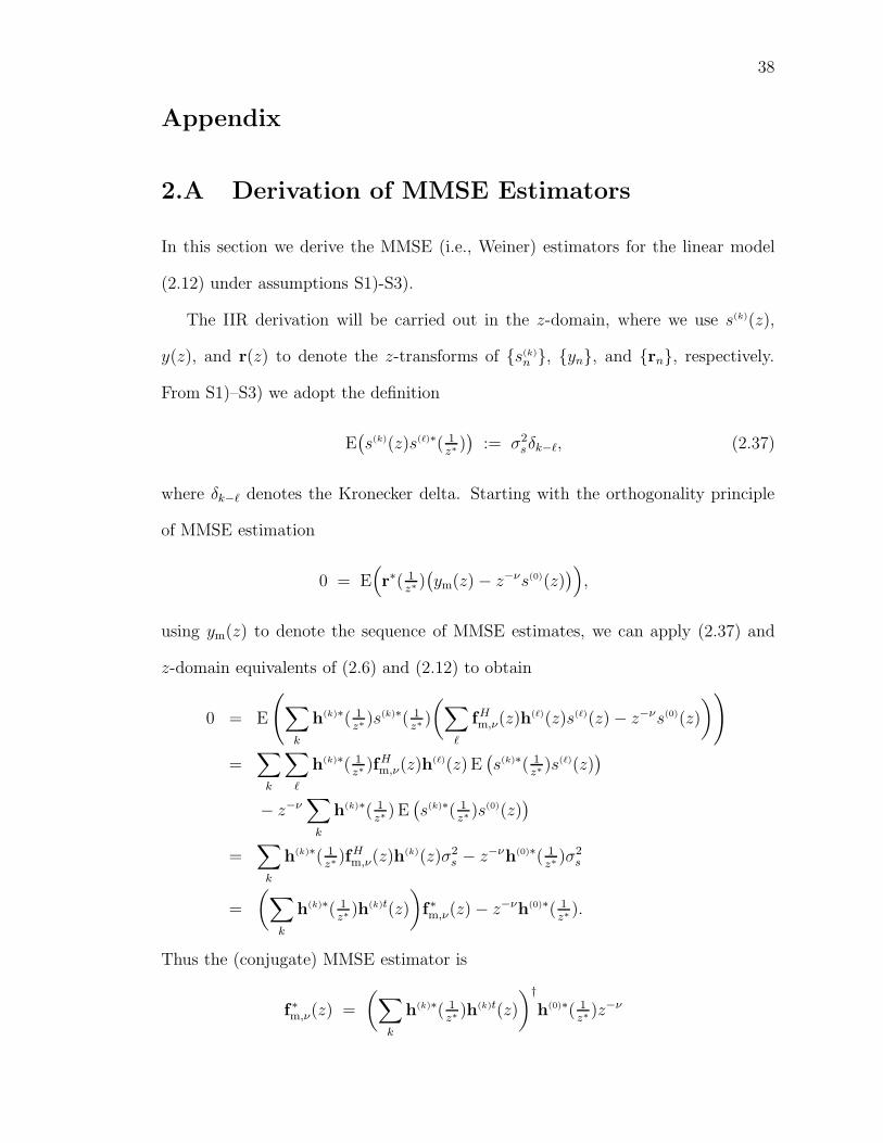
38

Appendix

2.A Derivation of MMSE Estimators

In this section we derive the MMSE (i.e., Weiner) estimators for the linear model

(2.12) under assumptions S1)-S3).

The IIR derivation will be carried out in the z-domain, where we use s(k)(z),

y(z), and r(z) to denote the z-transforms of {s(k)n }, {yn}, and {rn}, respectively.

From S1)–S3) we adopt the definition

E(s(k)(z)s(`)∗( 1

z∗))

:= σ2sδk−`, (2.37)

where δk−` denotes the Kronecker delta. Starting with the orthogonality principle

of MMSE estimation

0 = E(

r∗( 1z∗

)(ym(z) − z−νs(0)(z)

))

,

using ym(z) to denote the sequence of MMSE estimates, we can apply (2.37) and

z-domain equivalents of (2.6) and (2.12) to obtain

0 = E

(∑

k

h(k)∗( 1z∗

)s(k)∗( 1z∗

)

(∑

`

fHm,ν(z)h

(`)(z)s(`)(z) − z−νs(0)(z)

))

=∑

k

∑

`

h(k)∗( 1z∗

)fHm,ν(z)h

(`)(z) E(s(k)∗( 1

z∗)s(`)(z)

)

− z−ν∑

k

h(k)∗( 1z∗

) E(s(k)∗( 1

z∗)s(0)(z)

)

=∑

k

h(k)∗( 1z∗

)fHm,ν(z)h

(k)(z)σ2s − z−νh(0)∗( 1

z∗)σ2

s

=

(∑

k

h(k)∗( 1z∗

)h(k)t(z)

)

f∗m,ν(z) − z−νh(0)∗( 1z∗

).

Thus the (conjugate) MMSE estimator is

f∗m,ν(z) =

(∑

k

h(k)∗( 1z∗

)h(k)t(z)

)†h(0)∗( 1

z∗)z−ν

39

which may be plugged into the z-domain equivalent of (2.11) to yield

q(`)

m,ν(z) = z−νh(0)H( 1z∗

)

(∑

k

h(k)(z)h(k)H( 1z∗

)

)†h(`)(z).

The FIR derivation is analogous, though performed in the time domain. Using

ym(n) to denote the MMSE estimates, the orthogonality principle can be stated as

0 = E(

r∗(n)(ym(n) − e(0)t

ν s(n)))

, (2.38)

then using (2.7), (2.11), (2.38), source assumptions S1)–S3), and the fact that r(n) =

Hs(n), we have

0 = E(

H∗s∗(n)

(fH

m,νHs(n) − e(0)tν s(n)

))

= H∗ E(s∗(n)st(n)

)H

tf∗m,ν − H

∗ E(s∗(n)st(n)

)e(0)

ν

= H∗H

tf ∗m,νσ

2s − H

∗e(0)

ν σ2s

= H∗H

tf ∗m,ν − H

∗e(0)

ν .

Thus the (conjugate) MMSE estimator is

f ∗m,ν =

(H

∗H

t)†

H∗e(0)

ν

which yields

qm,ν = Htf ∗

m,ν = Ht(H

∗H

t)†

H∗e(0)

ν .

Chapter 3

Bounds for the MSE performance

of SW Estimators1

3.1 Introduction

It was proven independently in [Donoho Chap 81] and [Shalvi TIT 90] that uncon-

strained linear estimators locally maximizing the SW criterion yield perfect blind

estimates of a single non-Gaussian i.i.d. source transmitted through a noiseless in-

vertible linear channel. In practical situations, however, we expect constrained

estimators, noise and/or interference of a potentially non-Gaussian nature, and pos-

sibly non-invertible channels. Are Shalvi-Weinstein (SW) estimators useful in these

cases? How do SW estimators compare to optimal (linear) estimators, say, in a

mean square sense?

For a finite impulse response (FIR), but otherwise unconstrained, estimator and

a noiseless FIR channel, Regalia and Mboup studied various properties of SW min-

imizers [Regalia TSP 99]. Though they provided evidence that the SW and MMSE

1The main results of this chapter also appear in the manuscript [Schniter TSP tbd2].

40

41

estimators are closely related in most cases, their approach did not lead to upper

bounds on the performance of the SW estimator.

Recently, Feng and Chi studied the properties of unconstrained infinite-dimen-

sional SW estimators of a non-Gaussian source in the presence of Gaussian noise

[Feng TSP 99], [Feng TSP 00]. Using a frequency-domain approach, they observed

relationships between the Weiner and SW estimators that bear similarity2 to the

time-domain relationships derived previously by Regalia and Mboup. The complex-

ity of the analytical relationships derived by Feng and Chi prevents their translation

into meaningful statements about the MSE performance of SW estimators, however.

In this chapter we study the performance of constrained ARMA SW estimators

under the assumptions of the model in Section 2.2: desired source with arbitrary

non-Gaussian distribution, interference with arbitrary distribution, and vector IIR

(or FIR) channels. The main contributions of this chapter are (i) a simple test for

the existence of a SW estimator for the desired source (defined more rigorously in

Section 3.2.1), and (ii) bounding expressions for the MSE of SW estimators that

are a function of the minimum MSE attainable under the same conditions. These

bounds, derived under the multi-source linear model of Section 2.2, provide a formal

link between the SW and Wiener estimators in a very general context.

The organization of the chapter is as follows. Section 3.2 derives bounds for the

MSE performance of SW estimators, Section 3.3 presents the results of numerical

simulations demonstrating the efficacy of our bounding techniques, and Section 3.4

concludes the chapter.

2Keep in mind that Regalia and Mboup studied constrained estimators in noiseless settingswhile Feng and Chi studied unconstrained estimators in noisy settings.

42

3.2 SW Performance under General Additive In-

terference

In this section we derive tight bounds for the UMSE of SW symbol estimators that

• have a closed-form expression,

• support arbitrary additive interference,

• support complex-valued channels and estimators, and

• support IIR (as well as FIR) channels and estimators.

Section 3.2.1 outlines our approach, Section 3.2.2 presents the main results, and

Section 3.2.3 comments on these results. Proof details appear in Appendix 3.A.

3.2.1 The SW-UMSE Bounding Strategy

Since yn = qts(n) for q∈Qa, source assumptions S1)-S5) imply that [Porat Book 94]

K(yn) =∑

k

‖q(k)‖44 K(k)

s (3.1)

σ2y = ‖q(k)‖2

2σ2s . (3.2)

This allows us to rewrite the SW criterion (2.33) as

maxq∈Qa∩Qs

∣∣∣∣

∑

k

‖q(k)‖44 K(k)

s

∣∣∣∣

where Qs denotes the set of unit-norm global responses: Qs := {q s.t. ‖q‖2 = 1}.

Though the SW criterion admits multiple solutions, we are only interested in

those that correspond to the estimation of the 0th user’s symbols at delay ν. We

43

define the set of global responses associated3 with the {user, delay} pair {0, ν} as

follows:

Q(0)

ν :=

{

q s.t. |q(0)

ν | > max(k,δ)6=(0,ν)

|q(k)

δ |}

.

The set4 of SW global responses associated with the {0, ν} pair is then defined by

the following local maxima:

{qsw,ν} :=

{

arg maxq∈Qa∩Qs

∣∣∣

∑

k

‖q(k)‖44 K(k)

s

∣∣∣

}

∩Q(0)

ν .

It is not possible to write general closed-form expressions for {qsw,ν}, making it

difficult to characterize their performance. In fact, Appendix 3.A.1 shows that

{qsw,ν} may be empty, though for the discussion below we assume that this is not

the case.

Consider a reference global response qr,ν ∈ Qa ∩ Qs ∩ Q(0)ν . In other words, qr,ν

is an attainable unit-norm response associated with user/delay {0, ν}. When qr,ν is

in the vicinity of a qsw,ν (the meaning of which will be made more precise later), we

know that

∣∣∣∣

∑

k

‖q(k)

sw,ν‖4

4K(k)

s

∣∣∣∣≥∣∣∣∣

∑

k

‖q(k)

r,ν‖4

4K(k)

s

∣∣∣∣

=∣∣K(yr)

∣∣.

Thus this qsw,ν lies in the following set of global responses:

Qsw(qr,ν) :={

q s.t.∣∣∣

∑

k

‖q(k)‖44 K(k)

s

∣∣∣ ≥

∣∣K(yr)

∣∣

}

∩ Q(0)

ν ∩Qs. (3.3)

from which an SW-UMSE upper bound may be computed:

Ju,ν(qsw,ν) ≤ maxq∈Qsw(qr,ν)

Ju,ν(q). (3.4)

3Note that under S1)–S3), a particular user/delay combination is “associated” with an estimateif and only if that user/delay contributes more energy to the estimate than any other user/delay.

4We refer to the SW responses as a set to avoid establishing existence or uniqueness of localmaxima within Q(0)

νat this time.

44

Note that (3.4) avoids explicit consideration of the admissibility constraints of

Qa; they are implicitly incorporated via reference qr,ν ∈ Qa. Also note that the

tightness of the upper bound (3.4) will depend on the size and shape of Qsw(qr,ν),

motivating careful choice of qr,ν. In the sequel we choose the scaled MMSE reference

qr,ν = qm,ν/‖qm,ν‖2(when qm,ν ∈ Q(0)

ν ) since it is an established benchmark with a

closed-form expression.

Two simplifications will ease the evaluation of bound (3.4). The first is the re-

moval of absolute value signs in the definition (3.3). Recognize that for q sufficiently

close to e(0)ν , sgn

(∑

k ‖q(k)‖44 K(k)

s

)= sgn

(K(k)

s

), in which case

∣∣∣∣

∑

k

‖q(k)‖44 K(k)

s

∣∣∣∣

= sgn(K(k)

s

)∑

k

‖q(k)‖44 K(k)

s . (3.5)

Our bounds will impose conditions that ensure this behavior.

Next, since both the SW and UMSE criteria are invariant to phase rotation of q

(i.e., scalar multiplication of q by ejφ for φ ∈ R), we can restrict the our attention to

the set of “de-rotated” global responses {q s.t. q(0)ν ∈ R+}. For de-rotated responses

q ∈ Qs ∩Q(0)ν , we know q(0)

ν =√

1 − ‖q‖22, which implies that such q are completely

described by their interference response q (as described in Section 2.3.2). Moreover,

these interference responses lie within Q(0)ν , the projection of Q(0)

ν ∩Qs onto {q}:

Q(0)

ν :={

q s.t.

√

1 − ‖q‖22 > max

(k,δ)6=(0,ν)|q(k)

δ |}

.

(See Fig. 3.1 for the construction of Q(0)ν , whose boundary is illustrated by the thick

shaded curves.) Using this parameterization, (2.31) and (3.2) imply

Ju,ν(qsw,ν)

σ2s

∣∣∣∣q∈Qs∩Q(0)

ν

=‖q‖2

2

1 − ‖q‖22

∑

k

‖q(k)‖44 K(k)

s

∣∣∣∣q∈Qs∩Q(0)

ν

=(1 − ‖q‖2

2

)2 K(0)

s +∑

k

‖q(k)‖44 K(k)

s . (3.6)

45

−1

−0.5

0

0.5

1−1 −0.5 0 0.5 1

−1

−0.8

−0.6

−0.4

−0.2

0

0.2

0.4

0.6

0.8

1

q2

q1

q 0

Figure 3.1: Q(0)ν , created by projecting Q(0)

ν ∩ Qs onto the interference space, is

illustrated here for the three-dimensional case. The boundary of Q(0)ν is demarcated

by the thick shaded curves.

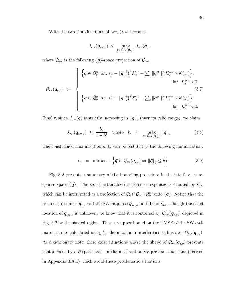
46

With the two simplifications above, (3.4) becomes

Ju,ν(qsw,ν) ≤ maxq∈Qsw(qr,ν)

Ju,ν(q).

where Qsw is the following {q}-space projection of Qsw:

Qsw(qr,ν) :=

{

q ∈ Q(0)ν s.t.

(1 − ‖q‖2

2

)2 K(0)

s +∑

k ‖q(k)‖44 K(k)

s ≥ K(yr)}

,

for K(0)

s > 0,

{

q ∈ Q(0)ν s.t.

(1 − ‖q‖2

2

)2 K(0)

s +∑

k ‖q(k)‖44 K(k)

s ≤ K(yr)}

,

for K(0)

s < 0.

(3.7)

Finally, since Ju,ν(q) is strictly increasing in ‖q‖2 (over its valid range), we claim

Ju,ν(qsw,ν) ≤ b2∗1 − b2∗

where b∗ := maxq∈Qsw(qr,ν)

‖q‖2. (3.8)

The constrained maximization of b∗ can be restated as the following minimization.

b∗ = min b s.t.{

q ∈ Qsw(qr,ν) ⇒ ‖q‖2 ≤ b}

(3.9)

Fig. 3.2 presents a summary of the bounding procedure in the interference re-

sponse space {q}. The set of attainable interference responses is denoted by Qa,

which can be interpreted as a projection of Qa ∩Qs ∩Q(0)ν onto {q}. Notice that the

reference response qr,ν and the SW response qsw,ν both lie in Qa. Though the exact

location of qsw,ν is unknown, we know that it is contained by Qsw(qr,ν), depicted in

Fig. 3.2 by the shaded region. Thus, an upper bound on the UMSE of the SW esti-

mator can be calculated using b∗, the maximum interference radius over Qsw(qr,ν).

As a cautionary note, there exist situations where the shape of Qsw(qr,ν) prevents

containment by a q-space ball. In the next section we present conditions (derived

in Appendix 3.A.1) which avoid these problematic situations.

47

Qsw(qr,ν)

Qa

qsw,ν

qr,ν

b∗

{q ∈ Q(0)ν }

Figure 3.2: Illustration of SW-UMSE bounding technique in the interference re-

sponse space {q}.

3.2.2 The SW-UMSE Bounds

In this section we present SW-UMSE bounds based on the method described in

Section 3.2.1. Proofs appear in Appendix 3.A.

Theorem 3.1. When K(ym), the kurtosis of estimates generated by the Wiener

estimator associated with the desired user at delay ν, obeys

K(0)

s ≥ K(ym) >(K(0)

s +Kmaxs

)/4, for K(0)

s > 0,

K(0)

s ≤ K(ym) <(K(0)

s +Kmins

)/4, for K(0)

s < 0,

(3.10)

the UMSE of SW estimators associated with the same user/delay can be upper

48

bounded by Ju,ν

∣∣max,K(ym)

sw,ν, where

Ju,ν

∣∣max,K(ym)

sw,ν:=

1−r

(ρmax+1)K(ym)

K(0)s

−ρmax

ρmax+r

(ρmax+1)K(ym)

K(0)s

−ρmax

σ2s , for K(0)

s > 0,

1−r

(ρmin+1)K(ym)

K(0)s

−ρmin

ρmin+r

(ρmin+1)K(ym)

K(0)s

−ρmin

σ2s , for K(0)

s < 0.

(3.11)

Furthermore, (3.10) guarantees the existence of a SW estimator associated with this

user/delay when q is FIR.

While Theorem 3.1 presents a closed-form SW-UMSE bounding expression in

terms of the kurtosis of the MMSE estimates, it is also possible to derive lower and

upper bounds in terms of the UMSE of the MMSE estimator.

Theorem 3.2. If Ju,ν(qm,ν) < Joσ2s , where

Jo :=

2√

(1 + ρmax)−1 − 1 K(0)

s > 0, Kmins ≥ 0

1−√

1−(3−ρmax)(1+ρmin)/4

ρmin+√

1−(3−ρmax)(1+ρmin)/4, K(0)

s > 0, Kmins < 0, Kmin

s 6= −K(0)

s

3−ρmax

5+ρmaxK(0)

s > 0, Kmins < 0, Kmin

s = −K(0)

s

2√

(1 + ρmin)−1 − 1 K(0)

s < 0, Kmaxs ≤ 0

1−√

1−(3−ρmin)(1+ρmax)/4

ρmax+√

1−(3−ρmin)(1+ρmax)/4, K(0)

s < 0, Kmaxs > 0, Kmax

s 6= −K(0)

s

3−ρmin

5+ρminK(0)

s < 0, Kmaxs > 0, Kmax

s = −K(0)

s

(3.12)

the UMSE of SW estimators associated with the same user/delay can be bounded as

follows:

Ju,ν(qm,ν) ≤ Ju,ν(qsw,ν) ≤ Ju,ν

∣∣max,K(ym)

sw,ν≤ Ju,ν

∣∣max,Ju,ν(qm,ν)

sw,ν,

49

where

Ju,ν

∣∣max,Ju,ν(qm,ν)

sw,ν:=

1−s

(1+ρmax)

„

1+Ju,ν(qm,ν)

σ2s

«−2

−ρmax

ρmax+

s

(1+ρmax)

„

1+Ju,ν(qm,ν)

σ2s

«−2

−ρmax

σ2s K(0)

s > 0, Kmins ≥ 0

1−s

(1+ρmax)

„

1+Ju,ν(qm,ν)

σ2s

«−2„

1+ρminJ2u,ν(qm,ν)

σ4s

«

−ρmax

ρmax+

s

(1+ρmax)

„

1+Ju,ν(qm,ν)

σ2s

«−2„

1+ρminJ2u,ν(qm,ν )

σ4s

«

−ρmax

σ2s K(0)

s > 0, Kmins < 0

1−s

(1+ρmin)

„

1+Ju,ν(qm,ν)

σ2s

«−2

−ρmin

ρmin+

s

(1+ρmin)

„

1+Ju,ν(qm,ν)

σ2s

«−2

−ρmin

σ2s K(0)

s < 0, Kmaxs ≤ 0

1−s

(1+ρmin)

„

1+Ju,ν(qm,ν)

σ2s

«−2„

1+ρmaxJ2u,ν(qm,ν)

σ4s

«

−ρmin

ρmin+

s

(1+ρmin)

„

1+Ju,ν(qm,ν)

σ2s

«−2„

1+ρmaxJ2u,ν(qm,ν)

σ4s

«

−ρmin

σ2s K(0)

s < 0, Kmaxs > 0.

(3.13)

Furthermore, (3.12) guarantees the existence of a SW estimator associated with this

user/delay when q is FIR.

Equation (3.13) leads to an elegant approximation of the extra UMSE of SW

estimators:

Eu,ν(qsw,ν) := Ju,ν(qsw,ν) − Ju,ν(qm,ν).

Theorem 3.3. If Ju,ν(qm,ν) < Joσ2s , then the extra UMSE of SW estimators can be

50

bounded as Eu,ν(qsw,ν) ≤ Eu,ν

∣∣max,Ju,ν(qm,ν)

c,ν, where

Eu,ν

∣∣max,Ju,ν(qm,ν)

c,ν

:= Ju,ν

∣∣max,Ju,ν(qm,ν)

sw,ν− Ju,ν(qm,ν)

=

12σ2

sρmaxJ

2u,ν(qm,ν) + O

(J3

u,ν(qm,ν))

K(0)

s > 0, Kmaxs ≥ 0

12σ2

s(ρmax − ρmin)J

2u,ν(qm,ν) + O

(J3

u,ν(qm,ν))

K(0)

s > 0, Kmaxs < 0

12σ2

sρminJ

2u,ν(qm,ν) + O

(J3

u,ν(qm,ν))

K(0)

s < 0, Kmaxs ≤ 0

12σ2

s(ρmin − ρmax)J

2u,ν(qm,ν) + O

(J3

u,ν(qm,ν))

K(0)

s < 0, Kmaxs > 0

(3.14)

Equation (3.14) implies that the extra UMSE of SW estimators is upper bounded

by approximately the square of the minimum UMSE. Fig. 3.3 plots the upper bound

on SW-UMSE and extra SW-UMSE from (3.13) as a function of Ju,ν(qm,ν)/σ2s for

various values of ρmin and ρmax. The second-order approximation based on (3.14)

appears very good for all but the largest values of UMSE.

3.2.3 Comments on the SW-UMSE Bounds

Implicit Incorporation of Qa

First, recall that the SW-UMSE bounding procedure incorporated Qa, the set of

attainable global responses, only in the requirement that qr,ν ∈ Qa ∩ Qs ∩ Q(0)ν .

Thus Theorems 3.1–3.3, written under the reference choice qr,ν = qm,ν/‖qm,ν‖2∈

Qa ∩Qs ∩Q(0)ν , implicitly incorporate the channel and/or estimator constraints that

define Qa. For example, if qm,ν is the MMSE response constrained to the set of

causal IIR estimators, then SW-UMSE bounds based on this qm,ν will implicitly

incorporate the causality constraint. The implicit incorporation of the attainable

set Qa makes these bounding theorems quite general and easy to use.

51

−80 −60 −40 −20 0−80

−70

−60

−50

−40

−30

−20

−10

0

UMSE(qm

) [dB]

UM

SE

[dB

]

(a)

−80 −60 −40 −20 0−160

−140

−120

−100

−80

−60

−40

−20

0

UMSE(qm

) [dB]

extr

a U

MS

E [d

B]

(b)

Ju(q

m)−based bound

Second−order approx

Ju(q

m)

Figure 3.3: Upper bound on (a) SW-UMSE and (b) extra SW-UMSE versus

Ju,ν(qm,ν) (when σ2s = 1) from (3.13) with second-order approximation from (3.14).

From left to right, {ρmin, ρmax} = {1000, 0}, {1,−2}, and {1, 0}.

52

Effect of ρmin and ρmax

When ρmin = 1 (as a result of K(0)

s < 0, Kmaxs ≤ 0, and Kmin

s = K(0)

s ) or when

ρmax = 1 (as a result of K(0)

s > 0, Kmins ≥ 0, and Kmax

s = K(0)

s ) the expressions in

Theorems 3.1–3.3 simplify:

Ju,ν(qsw,ν) ≤1 −

√

2K(ym)

K(0)s

− 1

1 +√

2K(ym)

K(0)s

− 1σ2

s when1

2<

K(ym)

K(0)

s

≤ 1,

≤1 −

√

2(

1 +Ju,ν(qm,ν)

σ2s

)−2

− 1

1 +

√

2(

1 +Ju,ν(qm,ν)

σ2s

)−2

− 1

σ2s when

Ju,ν(qm,ν)

σ2s

<√

2 − 1,

= Ju,ν(qm,ν) +1

2σ2s

J2u,ν(qm,ν) + O

(J3

u,ν(qm,ν)).

Note that in these cases, the SW-UMSE upper bound is independent of the specific

distribution of the desired and interfering sources, respectively.

In data communication applications, the case ρmin = 1 is typical as it results

from, e.g.,

a) sub-Gaussian desired source in the presence of Gaussian noise, or

b) constant-modulus desired source in the presence of non-super-Gaussian inter-

ference.

The case ρmin > 1, on the other hand, might arise from a non-CM (and possibly

shaped) desired source constellations in the presence of interference that is “more

sub-Gaussian.” In fact, source assumption S4) allows for arbitrarily large ρmin, which

could result from a nearly-Gaussian desired source in the presence of non-Gaussian

interference. Though Theorems 3.1–3.3 remain valid for arbitrarily high ρmin, the

requirements placed on Wiener performance (via Jo) become more stringent (recall

Fig. 3.3).

53

Generalization of Perfect SW-Estimation Property

Finally, we note that the Ju,ν(qm,ν)-based SW-UMSE bound in Theorem 3.2 implies

that the perfect SW-estimation property, proven under more restrictive conditions

in [Shalvi TIT 90], extends to the general multi-source linear model of Fig. 2.3:

Corollary 3.1. SW estimators are perfect (up to scaling) when Wiener estimators

are perfect.

Proof. From Theorem 3.2, Ju,ν(qm,ν) = 0 ⇒ Ju,ν(qsw,ν) = 0. Hence, the estimators

are perfect up to a (fixed) scale factor.

3.3 Numerical Examples

Here we present the results of experiments which compare the UMSE bounds of

Theorem 3.1 and Theorem 3.2 with the UMSE characterizing SW estimators found

by gradient descent5 under various source/interference environments. In all exper-

iments, ten non-Gaussian sources are mixed using a matrix H whose entries are

generated randomly from a real-valued zero-mean Gaussian distribution. The es-

timator f observes the mixture in the presence of AWGN (at SNR of 40dB) and

generates estimates of a particular source using Nf = 8 adjustable parameters.

Note that the number of sensors is less than the number of sources and that noise

is present, implying that H is not full column rank and perfect estimation is not

possible.

Figs. 3.4(a)–3.7(a) plot the UMSE upper bounds Ju,ν

∣∣max,K(ym)

sw,νand

Ju,ν

∣∣max,Ju,ν(qm,ν)

sw,νfor comparison with Ju,ν(qsw,ν). As a means of “zooming in” on the

5Gradient descent results were obtained by the Matlab routine “fmincon,” which was initial-

ized randomly in a small ball around the MMSE estimator.

54

small differences in UMSE, Figs. 3.4(b)–3.7(b) plot the extra-UMSE upper bounds

Eu,ν

∣∣max,K(qm,ν)

c,νand Eu,ν

∣∣max,Ju,ν(qm,ν)

c,ν. In all plots, the Ju,ν(qm,ν)-based bounds are de-

noted by solid lines, the K(qm,ν)-based bounds are denoted by •’s, and the gradient-

descent values are denoted by ×’s.

In Fig. 3.4 ten BPSK sources (i.e., K(k)

s = −2) mix with Gaussian noise. Note,

from Fig. 3.4(a), the tightness of the bounds for all but the largest values of

Ju,ν(qm,ν).

−30 −20 −10 0−30

−25

−20

−15

−10

−5

0

5

10

UMSE(qm

) [dB]

UM

SE

[dB

]

(a)

Ju(q

m)−based bound

K(ym

)−based bound

SW (grad descent)

−30 −20 −10 0−100

−90

−80

−70

−60

−50

−40

−30

−20

−10

0

UMSE(qm

) [dB]

extr

a U

MS

E [d

B]

(b)

Figure 3.4: Bounds on SW-UMSE for Nf = 8, 10 BPSK sources, AWGN at -40dB,

and random H.

Fig. 3.5 considers ten super-Gaussian sources, with K(k)

s = 2, in the presence

of Gaussian noise. From (3.13) we do not expect SW performance to differ from

55

the BPSK case (where K(k)

s = −2), and this notion is confirmed by comparison of

Fig. 3.4 and Fig. 3.5.

−30 −20 −10 0−30

−25

−20

−15

−10

−5

0

5

10

UMSE(qm

) [dB]

UM

SE

[dB

](a)

Ju(q

m)−based bound

K(ym

)−based bound

SW (grad descent)

−30 −20 −10 0−100

−90

−80

−70

−60

−50

−40

−30

−20

−10

0

UMSE(qm

) [dB]

extr

a U

MS

E [d

B]

(b)

Figure 3.5: Bounds on SW-UMSE for Nf = 8, 10 sources with K(k)

s = 2, AWGN at

-40dB, and random H.

Fig. 3.6 examines the estimation of a near-Gaussian signal (K(0)

s = 0.1) in the

presence of BPSK and AWGN interference. Comparing this experiment to the pre-

vious two, notice that here Ju,ν

∣∣max,K(ym)

sw,νis appreciably tighter than Ju,ν

∣∣max,Ju,ν(qm,ν)

sw,ν

for larger values of Ju,ν(qm,ν).

Finally, Fig. 3.7 examines the performance of a super-Gaussian signal (K(0)

s = 1)

in the presence of impulsive-type noise (K(k)

s = 100). When ρmax � 1, (3.10) and

(3.12) imply that we can only guarantee the existence of SW estimators in situations

56

−30 −20 −10 0−30

−25

−20

−15

−10

−5

0

5

10

UMSE(qm

) [dB]

UM

SE

[dB

]

(a)

Ju(q

m)−based bound

K(ym

)−based bound

SW (grad descent)

−30 −25 −20 −15 −10 −5−70

−60

−50

−40

−30

−20

−10

0

UMSE(qm

) [dB]

extr

a U

MS

E [d

B]

(b)

Figure 3.6: Bounds on SW-UMSE for Nf = 8, 5 BPSK sources, 5 sources with

K(k)

s = 0.1 (one of which is desired), AWGN at -40dB, and random H.

57

where MMSE estimates are relatively good. As the interference environment in this

experiment corresponds to ρmax = 100, UMSE bounds exist only when Ju,ν(qm,ν) <

−23 dB.

−35 −30 −25 −20−34

−32

−30

−28

−26

−24

−22

−20

−18

−16

UMSE(qm

) [dB]

UM

SE

[dB

]

(a)

Ju(q

m)−based bound

K(ym

)−based bound

SW (grad descent)

−35 −30 −25 −20−90

−80

−70

−60

−50

−40

−30

−20

UMSE(qm

) [dB]

extr

a U

MS

E [d

B]

(b)

Figure 3.7: Bounds on SW-UMSE for Nf = 8, 5 sources with K(k)

s = 100, 5 sources

with K(k)

s = 1 (one of which is desired), AWGN at -40dB, and random H.

3.4 Conclusions

In this chapter we have derived conditions under which SW estimators exist and

derived bounds for the UMSE of SW estimators. The existence conditions are simple

tests which guarantee a SW estimator for the desired user at a particular delay,

58

and these existence arguments have been proven for vector-valued FIR channels

and constrained vector-valued FIR estimators. The UMSE bounds hold for vector-

valued FIR/IIR channels, constrained FIR/IIR estimators, and nearly arbitrary

source and interference distributions. The first bound is a function of the kurtosis

of the MMSE estimates, while the second bound is a function of the minimum UMSE

of MMSE estimators. Analysis of the second bound shows that the extra UMSE

of SW estimators is upper bounded by approximately the square of the minimum

UMSE. Thus, SW estimators are very close (in a MSE sense) to optimum linear

estimators when the minimum MSE is small. Numerical simulations suggest that

the bounds are reasonably tight.

59

Appendix

3.A Derivation Details for SW-UMSE Bounds

This appendix contains the proofs of the theorems and lemmas found in Section 3.2.

3.A.1 Proof of Theorem 3.1

In this section, we are interested in deriving an expression for the interference radius

b∗ defined in (3.9) and establishing conditions under which this radius is well defined.

Rather than working with (3.9) directly, we find it easier to use the equivalent

definition

b∗ = min b s.t.{

‖q‖2 > b⇒ q /∈ Qsw(qr,ν)}

(3.15)

= min b s.t.

{

‖q‖2 > b ⇒(1 − ‖q‖2

2

)2 K(0)

s +∑

k ‖q(k)‖44 K(k)

s < K(yr)}

,

when K(0)

s > 0,{

‖q‖2 > b ⇒(1 − ‖q‖2

2

)2 K(0)

s +∑

k ‖q(k)‖44 K(k)

s > K(yr)}

,

when K(0)

s < 0.

We handle the super-Gaussian case (i.e., K(0)

s > 0) first. The following statements

are equivalent.

K(yr) >(1 − ‖q‖2

2

)2 K(0)

s +∑

k

‖q(k)‖44 K(k)

s

0 >

(

1 − K(yr)

K(0)

s

)

︸ ︷︷ ︸

Cr

−2‖q‖22 + ‖q‖4

2 +∑

k

‖q(k)‖44

K(k)

s

K(0)

s

(3.16)

Now using the fact that

∑

k

‖q(k)‖44 K(k)

s ≤∑

k

‖q(k)‖44 Kmax

s ≤∑

k

‖q(k)‖42 Kmax

s = ‖q‖42 Kmax

s , (3.17)

60

and the definition of ρmax, the following is a sufficient condition for (3.16):

0 > (1 + ρmax)‖q‖42 − 2‖q‖2

2 + Cr. (3.18)

Since 1 + ρmax > 0, the set of {‖q‖22} satisfying (3.18) is equivalent to the set of

points {x} that lie between the roots {x1, x2} of the quadratic

P2(x) = (1 + ρmax)x2 − 2x+ Cr.

Because q is an interference response, we need not consider all values of ‖q‖2. As

explained below, we only need to concern ourselves about 0 ≤ ‖q‖2 <√

2−1

. This

implies that a valid upper bound on b2∗ is given by the smaller root of P2(x) when

(i) this smaller root is non-negative real and (ii) the larger root of P2(x) is ≥ 0.5.

When both roots of P2(x) lie in the interval [0, 0.5), there exist two valid regions

in the interference space with absolute kurtosis larger than at the reference, i.e.,

Qsw(qr,ν) becomes disjoint. The “inner” part of Qsw(qr,ν) allows UMSE bounding

since it can be contained by {q : ‖q‖2 ≤ b1} for a positive interference radius b1, but

the “outer” part of Qsw(qr,ν) does not permit UMSE bounding in this manner. As

an example of this behavior, Fig. 3.8(a) plots the quadratic P2(x) and Fig. 3.8(b) the

region Qsw(qr,ν) in two-dimensional interference space. As in Fig. 3.2, the attainable

set Qa is denoted by the curved line, the boundary of valid interference region Q(0)ν

by the dotted lines, the SW response by the dot, and the reference response by the

diamond. Q(0)ν is the projection of Q(0)

ν ∩ Qs onto {q}.

Disjointness of Qsw(qr,ν) arises from an interfering source k 6= 0 such that

| K(k)

s | > | K(0)

s |. In these scenarios, the point of highest kurtosis in the “outer”

regions of Qsw(qr,ν) occurs at points near the boundary of Q(0)ν of the form q =

(. . . , 0, 0, ejθ√

2−1, 0, 0, . . . )t. Thus, when x2 ≥ 0.5, we can be assured that all valid

interference responses (i.e., q ∈ Q(0)ν ) with kurtosis greater than the reference can

61

0 0.1 0.2 0.3 0.4 0.5−0.1

0

0.1

0.2

0.3

0.4

0.5

0.6

0.7

x=||qbar||22

P2(x

)

(a)

−0.5 0 0.5−0.8

−0.6

−0.4

−0.2

0

0.2

0.4

0.6

0.8

qbar1

qbar

2

(b)

Figure 3.8: Example of P2(x) and disjoint Qsw(qr,ν) when larger root of P2(x) is

< 0.5.

be bounded by some radius b1. In contrast to Fig. 3.8, Fig. 3.9 demonstrates a

situation where both root requirements are satisfied.

The roots of P2(x) are given by

{x1, x2} =1 ±

√

1 − (1 + ρmax)Cr

1 + ρmax

, assuming x1 ≤ x2,

which are both non-negative real when 0 ≤ Cr ≤ (1+ρmax)−1. It can be shown that

x2 ≥ 0.5 when Cr ≤ (3−ρmax)/4. Since ρmax ≥ 1 implies (3−ρmax)/4 ≤ (1+ρmax)−1,

both root requirements are satisfied when 0 ≤ Cr ≤ (3 − ρmax)/4, or equivalently

when

K(0)

s ≥ K(yr) ≥(K(0)

s +Kmaxs

)/4. (3.19)

Notice that when (3.19) is satisfied, the facts K(0)

s > 0 and (K(0)

s +Kmaxs ) > 0 imply

sgn(K(0)

s ) = sgn(K(yr)), thus confirming the validity of (3.5).

Under satisfaction of (3.19), equation (3.8) implies the following bound for the

62

0 0.1 0.2 0.3 0.4 0.5−0.1

−0.05

0

0.05

0.1

0.15

0.2

0.25

x=||qbar||22

P2(x

)

(a)

−0.5 0 0.5−0.8

−0.6

−0.4

−0.2

0

0.2

0.4

0.6

0.8

qbar1

qbar

2

(b)

Figure 3.9: Example of P2(x), Qsw(qr,ν), and bounding radius when larger root of

P2(x) is > 0.5.

super-Gaussian case:

Ju,ν(qsw,ν) ≤ b2∗1 − b2∗

≤ x21

1 − x21

=1 −

√

(1 + ρmax)K(yr)

K(0)s

− ρmax

ρmax +√

(1 + ρmax)K(yr)

K(0)s

− ρmax

when K(0)

s > 0. (3.20)

The difference between b∗ and x1 accounts for the space between Qsw(qr,ν) and the

bounding radius in Fig. 3.9.

As for the existence of an attainable SW global response associated with the

desired user at delay ν, i.e., qsw,ν ∈ Qa ∩ Qs ∩ Q(0)ν , we work in the q space and

establish the existence of a kurtosis local maximum qsw,ν in the set Qa ∩ Q(0)ν . For

simplicity, we assume that the space q is finite dimensional. We will exploit the

Weierstrass theorem [Luenberger Book 69, p. 40], which says that a continuous cost

functional must have a local maximum on a compact set if there exist points in the

63

interior of the set which give cost strictly higher than anywhere on the boundary.

The approach is illustrated in Fig. 3.10.

By definition, all points in Qsw(qr,ν) give kurtosis ≥ K(yr), the kurtosis ev-

erywhere on the boundary of Qsw(qr,ν). To make this inequality strict, we ex-

pand Qsw(qr,ν) to form the new set Q′sw(qr,ν) defined in terms of boundary kurtosis

K(yr)− ε (for arbitrarily small ε > 0). Thus, all points on the boundary of Q′sw(qr,ν)

will give kurtosis strictly less than K(yr). But how do we know that such a set

Q′sw(qr,ν) exists? We simply need to reformulate (3.16) with ε-smaller K(yr), result-

ing in ε-larger Cr and a modified quadratic P2(x) in sufficient condition (3.18). As

long as the new roots (call them x′1 and x′2) satisfy x′1 ∈ [0, 0.5) and x′2 > 0.5, the

set Q′sw(qr,ν) is well defined. This property can be guaranteed, for arbitrarily small

ε, by replacing (3.19) with the stricter condition

K(0)

s ≥ K(yr) >(K(0)

s +Kmaxs

)/4. (3.21)

To summarize, (3.21) guarantees the existence of a closed and bounded set

Q′sw(qr,ν) ⊂ Q(0)

ν containing an interior point qr,ν with kurtosis strictly greater than

all points on the set boundary.

Due to attainability requirements, our local maximum search must be con-

strained to the relative interior of the Qa manifold (which has been embedded in

a possibly higher-dimensional q-space; see Fig. 3.10 for an illustration of a one-

dimensional Qa embedded in R2). Can we apply the Weierstrass theorem on this

manifold? First, we know the Qa manifold intersects Q′sw(qr,ν), namely at the point

qr,ν. Second, we know that the relative boundary of the Qa manifold occurs out-

side Q′sw(qr,ν), namely at infinity. These two observations imply that the boundary

of Qa ∩ Q′sw(qr,ν) relative to Qa must be a subset of the boundary of Q′

sw(qr,ν).

Hence, the interior of Qa ∩ Q′sw(qr,ν) relative to Qa contains points which give kur-

64

tosis strictly higher than those on the boundary of Qa ∩ Q′sw(qr,ν) relative to Qa.

(See Fig. 3.10 for an illustration of these relationships.) Finally, the domain (i.e.,

Qa∩Q′sw(qr,ν) relative to Qa) is closed and bounded, hence compact. Thus the Weier-

strass theorem ensures the existence of a local kurtosis maximum in the interior of

Qa ∩Q′sw(qr,ν) relative to Qa under (3.21). Recalling the one-to-one correspondence

between points in Qa ∩ Q′sw(qr,ν) and points in Qa ∩Qs ∩Q′

sw(qr,ν), there exists an

attainable SW response for the desired user/delay: qsw,ν ∈ Qa ∩ Qs ∩ Q(0)ν .

x′1

Qa

bndr Q′sw(qr,ν)

bndr Qsw(qr,ν)

bndr Qa relative to Qa

bndr(Qa ∩ Q′

sw(qr,ν))

relative to Qa

qr,ν

Figure 3.10: Illustration of local minima existence arguments.

Using a similar development for the sub-Gaussian case, we find that when

K(0)

s ≤ K(yr) <(K(0)

s +Kmins

)/4, (3.22)

the UMSE of SW estimators can be bounded as follows:

Ju,ν(qsw,ν) ≤1 −

√

(1 + ρmin)K(yr)

K(0)s

− ρmin

ρmin +√

(1 + ρmin)K(yr)

K(0)s

− ρmin

when K(0)

s < 0. (3.23)

Furthermore, (3.22) implies that a SW estimator exists within Qa ∩ Qs ∩ Q(0)ν .

Choosing the scaled Weiner reference qr,ν = qm,ν/‖qm,ν‖2in equations (3.20)–

(3.23) gives Theorem 3.1. Note that we only consider the case qm,ν ∈ Q(0)ν .

65

3.A.2 Proof of Theorem 3.2

From Appendix 3.A.1, we know that the expressions in Theorem 3.1 hold for any

reference estimates associated with the desired source at delay ν. We consider the

case of a super-Gaussian source (i.e., K(0)

s > 0) first. Noting that Ju,ν

∣∣max,K(yr)

sw,νin

(3.11) is a strictly decreasing function of K(yr)/K(0)

s (over its valid range), an upper

bound for Ju,ν

∣∣max,K(yr)

sw,νfollows from a lower bound of K(yr)/K(0)

s . From (3.6),

K(yr)

K(0)

s

=(1 − ‖qr,ν‖2

2

)2+∑

k

‖q(k)

r,ν‖4

4

K(k)

s

K(0)

s

≥(1 − ‖qr,ν‖2

2

)2+

Kmins

K(0)

s

‖qr,ν‖4

4

≥

1 − 2‖qr,ν‖2

2+ ‖qr,ν‖4

2, Kmin

s ≥ 0,

1 − 2‖qr,ν‖2

2+ (1 + ρmin)‖qr,ν‖4

2, Kmin

s < 0.

When K(0)

s > 0 and Kmins ≥ 0, we see that

1 − 2‖qr,ν‖2

2+ ‖qr,ν‖4

2=

(1 − ‖qr,ν‖2

2

)2

=

(

1 +‖qr,ν‖2

2

1 − ‖qr,ν‖2

2

)−2

=

(

1 +Ju,ν(qr,ν)

σ2s

)−2

which implies the bound

Ju,ν

∣∣max,K(yr)

sw,ν≤

1 −√

(1 + ρmax)(

1 +Ju,ν(qr,ν)

σ2s

)−2

− ρmax

ρmax +

√

(1 + ρmax)(

1 +Ju,ν(qr,ν)

σ2s

)−2

− ρmax

(3.24)

as long as

1 ≥ K(yr)

K(0)

s

>1 + ρmax

4. (3.25)

Having just shown that K(yr)/K(0)

s ≥ (1+Ju,ν(qr,ν)/σ2s)

−2, a sufficient condition for

the right inequality of (3.25) is (1 + Ju,ν(qr,ν)/σ2s)

−2 > (1 + ρmax)/4 which can be

66

restated as

Ju,ν(qr,ν)

σ2s

< − 1 + 2√

(1 + ρmax)−1. (3.26)

For the left inequality in (3.25), we use (3.6) and (3.17) to bound

K(yr)

K(0)

s

≤ 1 − 2‖qr,ν‖2

2+ (1 + ρmax)‖qr,ν‖4

2

=(1 − ‖qr,ν‖2

2

)2(

1 + ρmax

‖qr,ν‖4

2(1 − ‖qr,ν‖2

2

)2

)

=

(

1 +Ju,ν(qr,ν)

σ2s

)−2(

1 + ρmax

J2u,ν(qr,ν)

σ4s

)

.

Thus 1 ≥ (1 + Ju,ν(qr,ν)/σ2s)

−2(1 + ρmaxJ2u,ν(qr,ν)/σ

4s) is sufficient for the left side of

(3.25), which can be restated simply as Ju,ν(qr,ν)/σ2s ≤ 2(ρmax − 1)−1. But, using

the fact that ρmax ≥ 1, it can be shown that −1 + 2√

(1 + ρmax)−1 ≤ 2(ρmax − 1)−1,

and thus (3.26) remains as a sufficient condition for bound (3.24).

For the case when K(0)

s > 0 and Kmins < 0, we have just shown that

K(yr)

K(0)

s

≥ 1 − 2‖qr,ν‖2

2+ (1 + ρmin)‖qr,ν‖4

2

=

(

1 +Ju,ν(qr,ν)

σ2s

)−2(

1 + ρmin

J2u,ν(qr,ν)

σ4s

)

,

which implies the bound

Ju,ν

∣∣max,K(yr)

sw,ν≤

1 −√

(1 + ρmax)(

1 +Ju,ν(qr,ν)

σ2s

)−2 (

1 + ρminJ2u,ν(qr,ν)

σ4s

)

− ρmax

ρmax +

√

(1 + ρmax)(

1 +Ju,ν(qr,ν)

σ2s

)−2 (

1 + ρminJ2u,ν(qr,ν)

σ4s

)

− ρmax

(3.27)

as long as (3.25) holds. A sufficient condition for the right inequality in (3.25) would

then be 1 − 2‖qr,ν‖2

2+ (1 + ρmin)‖qr,ν‖4

2> (1 + ρmax)/4, or equivalently

(1 + ρmin)‖qr,ν‖4

2− 2‖qr,ν‖2

2+ (3 − ρmax)/4 > 0.

67

It can be shown that the quadratic inequality above is satisfied by

‖qr,ν‖2

2<

1−√

1−(3−ρmax)(1+ρmin)/4

1+ρmin, ρmin 6= −1,

(3 − ρmax)/8 ρmin = −1,

and since Ju,ν(q) = ‖q‖22/(1−‖q‖2

2) is strictly increasing in ‖q‖22, the following must

be sufficient for the right inequality of (3.25).

Ju,ν(qr,ν)

σ2s

<

1−√

1−(3−ρmax)(1+ρmin)/4

ρmin+√

1−(3−ρmax)(1+ρmin)/4, ρmin 6= −1,

3−ρmax

5+ρmaxρmin = −1.

(3.28)

For the left inequality in (3.25) we have the same sufficient condition as when K(0)

s >

0 and Kmins ≥ 0, namely, Ju,ν(qr,ν)/σ

2s ≤ 2(ρmax − 1)−1. Again, this latter condition

is less stringent than (3.28), implying that (3.28) is sufficient for bound (3.27).

The case of a sub-Gaussian source can be treated in a similar manner, and

the results are the same as (3.24), (3.26), (3.27), and (3.28), modulo a swapping

of ρmin and ρmax. The final results are collected in Theorem 3.2 under the choice

qr,ν = qm,ν/‖qm,ν‖2. The UMSE conditions above guarantee that qm,ν ∈ Q(0)

ν .

3.A.3 Proof of Theorem 3.3

Here, we reformulate the upper bound (3.13). To simplify the presentation of the

proof, the shorthand notation J := Ju,ν(qm,ν)/σ2s will be used.

Starting with the case that K(0)

s > 0 and Kmins ≥ 0, (3.13) says

Ju,ν

∣∣max,Ju,ν(qm,ν)

sw,ν

σ2s

=1 −

√

(1 + ρmin)(1 + J)−2 − ρmin

ρmin +√

(1 + ρmin)(1 + J)−2 − ρmin

,

from which routine manipulations yield

Ju,ν

∣∣max,Ju,ν(qm,ν)

sw,ν

σ2s

=1 −

√

1 −((ρmin − 1) + ρmin(2J + J2)

)(2J + J2)

(ρmin − 1) + ρmin(2J + J2).

68

For x ∈ R such that |x| < 1, the binomial series [Rudin Book 76] may be used to

claim

√1 − x = 1 − x

2− x2

8−O(x3).

Applying the previous expression with x =((ρmin − 1) + ρmin(2J + J2)

)(2J + J2),

we find that

Ju,ν

∣∣max,Ju,ν(qm,ν)

sw,ν

σ2s

=1

2

((ρmin − 1) + ρmin(2J + J2)

)(2J + J2)

(ρmin − 1) + ρmin(2J + J2)

+1

8

((ρmin − 1) + ρmin(2J + J2)

)2(2J + J2)2

(ρmin − 1) + ρmin(2J + J2)+ O(J3)

= J +ρmin

2J2 + O(J3).

Finally, subtraction of J gives the first case in (3.14).

For the case of K(0)

s > 0 and Kmins < 0, (3.13) says

Ju,ν

∣∣max,Ju,ν(qm,ν)

sw,ν

σ2s

=1 −

√

(1 + ρmin)(1 + J)−2(1 + ρmaxJ2) − ρmin

ρmin +√

(1 + ρmin)(1 + J)−2(1 + ρmaxJ2) − ρmin

,

from which routine manipulations yield

Ju,ν

∣∣max,Ju,ν(qm,ν)

sw,ν

σ2s

=

ρmaxJ2 + 1 −

√

1 + (2 − 2ρmax)J + (1 + ρmax + ρminρmax − 5ρmin)J2 + O(J3)

(ρmin − 1) + 2ρminJ + (ρmin − ρmax)J2.

As before, we use the binomial series expansion for√

1 − x, but now with x =

(2ρmax −2)J +(5ρmin−1−ρmax −ρminρmax)J2 +O(J3). After some algebra, we find

Ju,ν

∣∣max,Ju,ν(qm,ν)

sw,ν

σ2s

= J +1

2

(ρmin − ρmax)(ρmin − 1)J2 + O(J3)

(ρmin − 1) + 2ρminJ + (ρmin − ρmax)J2

Finally we apply the series approximation

1

1 − y= 1 + y + O(y2)

69

with y = −(2ρminJ + (ρmin − ρmax)J2)/(ρmin − 1) for ρmin 6= 1. Straightforward

algebra yields

Ju,ν

∣∣max,Ju,ν(qm,ν)

sw,ν

σ2s

= J +1

2(ρmin − ρmax)J

2 + O(J3).

Taking the limit ρmin → 1, it is evident that no problems arise at the point ρmin = 1.

Subtraction of J from the last statement gives the second case in (3.14).

Chapter 4

Bounds for the MSE performance

of CM Estimators1

4.1 Introduction

Under “ideal” conditions, CM-minimizing estimators are perfect modulo unavoid-

able gain and delay ambiguities. In other words, CM-minimizing {yn} = {αs(0)

n−ν}

for some α and ν. More specifically, for a single source satisfying S1), S4) and S5),

the perfect CM-estimation property has been proven for

• unconstrained doubly-infinite estimators with BIBO channels:

[Foschini ATT 85], and

• causal FIR estimators with full-column rank (FCR) H: [Tong CISS 92],

[Li TSP 96a].

(As we show in Section 4.2.3, the perfect CM-estimation property can also be ex-

tended to the multi-source linear model described in Section 2.2.) But how good

1The main results of this chapter also appear in the manuscript [Schniter TIT 00].

70

71

are CM-minimizing estimators under non-ideal conditions?

The last decade has seen a plethora of papers giving evidence for the “robustness”

of CM performance in situations where the CM-minimizing (and MMSE) estimators

are not perfect. Most of these studies, however, focus on particular features of the

system model that prevent perfect estimation, such as

1. the presence of additive white Gaussian noise (AWGN) corrupting the obser-

vation (e.g., [Fijalkow TSP 97], [Zeng TIT 98], [Liu SP 99]),

2. channels that do not provide adequate diversity (e.g., [Fijalkow TSP 97],

[Li TSP 96b]), or

3. estimators with an insufficient number of adjustable parameters (e.g.,

[Endres TSP 99], [Regalia TSP 99]).

A notable exception is the work of Zeng et al. [Zeng TSP 99], in which an algorithm

is given to bound the MSE of CM-minimizing estimators for the case of a single

source transmitted through a finite-duration impulse response (FIR) linear channel

in the presence of AWGN. The channel model assumed by [Zeng TSP 99] is general

enough to incorporate most combinations of the three conditions above, though

not as general as the multi-source model of Fig. 2.3. The bounding algorithm in

[Zeng TSP 99] is rather involved, however, preventing a direct link between the MSE

performance of CM and Wiener estimators. (See Table 4.1.)

The main contribution of this chapter is a (closed-form) bound on the MSE

performance of CM-minimizing estimators that is a simple function of the MSE

performance of Weiner estimators. This bound, derived under the multi-source

linear model in Section 2.2, provides the most formal link (established to date)

between the CM and Wiener estimators, and as such, the most general testament

72

to the MSE-robustness of the CM criterion.

The organization of the chapter is as follows. Section 4.2 derives the bound

for the MSE performance of the CM criterion, Section 4.3 presents the results of

numerical simulations demonstrating the efficacy of our bounding technique, and

Section 4.4 concludes the chapter.

4.2 CM Performance under General Additive In-

terference

An algorithm for bounding the MSE performance of CM minimizers has been derived

by Zeng et al. for the case of a real-valued i.i.d. source, a FIR channel, AWGN, and

a finite-length estimator. The development for FCR and non-FCR H appear in

[Zeng TIT 98] and [Zeng TSP 99], respectively. Using the notation established in

Section 2.2, the algorithm of [Zeng TSP 99] is summarized in Table 4.1. Though the

relatively complicated Zeng algorithm generates reasonably tight CM-UMSE upper

bounds (as we shall see in Section 4.3), we have found that it is possible to derive

tight bounds for the UMSE of CM-minimizing symbol estimators that

• have a closed-form expression,

• support arbitrary additive interference,

• support complex-valued channels and estimators, and

• support IIR (as well as FIR) channels and estimators.

We will now derive such bounds. Section 4.2.1 outlines our approach, Sec-

tion 4.2.2 presents the main results, and Section 4.2.3 comments on these results.

Proof details appear in Appendix 4.A.

73

Table 4.1: Zeng et al.s’ CM-UMSE bounding algorithm [Zeng TSP 99].

Assumptions:

The desired (k = 0) channel is FIR with coefficients {h(0)

i } ∈ RP .AWGN of variance σ2

w is present at each of P sensors, so that

rn =∑Nh−1

i=0

(

h(0)

i s(0)

n−i + σw

σs

∑Pk=1 eks

(k)

n−i

)

.

The sources are real-valued and satisfy (S1)-(S5).The dispersion constant is γ = E{|s(0)

n |4}/σ2s .

The estimator f = (f t0, . . . , f

tNf−1)

t has Nf coefficients of size P × 1.

Definitions:

H :=

(h

(0)0 h

(0)1 ... h

(0)Nh−1...

...h

(0)0 h

(0)1 ... h

(0)Nh−1

)

∈ RPNf×(Nf +Nh−1).

R := HHt + (σw

σs)2I.

Φ := I + (σw

σs)2 (HtH)

†=

(C11 b1 C12

bt1 a b

t2

C12 b2 C22

)

,

set a := [Φ]ν,ν , b :=(

b1b2

)and C :=

(C11 C12C12 C22

).

Calculations:

q(0)m,ν = HtR−1Heν .

q(0)

mI = q(0)m,ν(0 : ν−1, ν+1 : Nq−1)/q(0)

m,ν(ν), using Matlab notation.

αr,ν =

√√√√ γ‖q(0)

m,ν‖2

Φ

3‖q(0)m,ν‖4

Φ− (3 − γ)‖q(0)

m,ν‖4

4

.

q(0)r,ν = αr,νq

(0)m,ν .

Jc,ν(q(0)r,ν) = 3‖q(0)

r,ν‖4

Φ− 2γ‖q(0)

r,ν‖2

Φ− (3 − γ)‖q(0)

r,ν‖4

4+ γ2.

q(0)

oI = −C−1b.θo = (a− btC−1b)−1.δo = ‖q(0)

mI − q(0)

oI ‖C.

UMSE Bound:

For the quartic polynomial D(δ) = c21(δ) − 4c2(δ)c0, wherec0 = γ2 − Jc,ν(q

(0)r,ν),

c1(δ) = −2γ(δ2 + θ−1o ),

c2(δ) = 3(δ2 + θ−1o )2 − (3 − γ)

(1 + (δ + ‖q(0)

oI ‖4)4),

find {δ1 < · · · < δm} = real-valued roots of D(δ), andset δ? = min{δi | δi > δo}.If δ? 6= ∅, D(δo) ≥ 0, and c2(δ) > 0 for all δ ∈ [δo, δ?], then

UMSE(q(0)c,ν) ≤ δ2

? + θ−1o − 1,

else unable to compute bound.

74

4.2.1 The CM-UMSE Bounding Strategy

Say that qr,ν is an attainable global reference response for the desired user (k = 0)

at some fixed delay ν. Formally, qr,ν ∈ Qa ∩ Q(0)ν , where

Q(0)

ν :=

{

q s.t. |q(0)

ν | > max(k,δ)6=(0,ν)

|q(k)

δ |}

.

Q(0)ν defines the set of global responses associated2 with user 0 at delay ν. The set3

of (attainable) locally CM-minimizing global responses for the desired user at delay

ν will be denoted by {qc,ν} and defined as:

{qc,ν} :=

{

arg minq∈Qa

Jc(q)

}

∩ Q(0)

ν .

In general, it is not possible to determine closed-form expressions for {qc,ν}, making

it difficult to evaluate the UMSE of CM-minimizing estimators.

When qr,ν is in the vicinity of a qc,ν (the meaning of which will be made more

precise later) then, by definition, this qc,ν must have CM cost less than or equal to

the cost at qr,ν. In this case, ∃qc,ν ∈ Qc(qr,ν), where

Qc(qr,ν) :={q s.t. Jc(q) ≤ Jc(qr,ν)

}∩ Q(0)

ν . (4.1)

This approach implies the following CM-UMSE upper bound:

Ju,ν(qc,ν) ≤ maxq∈Qc(qr,ν)

Ju,ν(q). (4.2)

Note that the maximization on the right of (4.2) does not explicitly involve the

admissibility constraint Qa; the constraint is implicitly incorporated through qr,ν.

The tightness of the upper bound (4.2) will depend on the size and shape of

Qc(qr,ν), motivating careful selection of the reference qr,ν. Notice that the size of

2Note that under S1)–S3), a particular {user, delay} combination is “associated” with an es-timate if and only if that {user, delay} contributes more energy to the estimate than any other{user, delay}.

3We refer to the CM-minimizing responses as a set to avoid establishing existence or uniquenessof local minima within Qa ∩ Q(0)

νat this time.

75

Qc(qr,ν) can usually be reduced via replacement of qr,ν with βrqr,ν , where βr :=

arg minβ Jc(βqr,ν). This implies that the direction (rather than the size) of qr,ν is

important; the tightness of the CM-UMSE bound (4.2) will depend on collinearity

of qr,ν and qc,ν . Fig. 4.1 presents an illustration of this idea.

Zeng has shown that in the case of an i.i.d. source, a FIR channel and AWGN

noise, qc,ν is nearly collinear to the MMSE response qm,ν [Zeng TSP 99]. These

findings, together with the abundant interpretations of the MMSE estimator and

the existence of closed-form expressions for qm,ν (e.g., (2.27) and (2.28)), suggest

the reference choice qr,ν = qm,ν .

Determining a CM-UMSE upper bound from (4.2) can be accomplished as fol-

lows. Since both Jc(q) and Ju,ν(q) are invariant to phase rotation of q (i.e., scalar

multiplication of q by ejφ for φ ∈ R), we can restrict our attention to the set of “de-

rotated” responses {q s.t. q(0)ν ∈ R+}. Such q allow parameterization in terms of gain

a = ‖q‖2 and interference response q (defined in Section 2.3.2), where ‖q‖2 ≤ a. In

terms of the pair (a, q), the upper bound in (4.2) may then be rewritten

maxq∈Qc(βrqr,ν)

Ju,ν(q) = maxa

(

maxq: (a,q)∈Qc(βrqr,ν)

Ju,ν(a, q)

)

.

Under particular conditions on the gain a and the reference qr,ν (made explicit in

Section 4.2.2), there exists a minimum interference gain

b∗(a) := min b(a) s.t.{

(a, q) ∈ Qc(βrqr,ν) ⇒ ‖q‖2 ≤ b(a)}

, (4.3)

which can be used in the containment:

{

(a, q) ∈ Qc(βrqr,ν)}

⊂{

(a, q) s.t. ‖q‖2 ≤ b∗(a)}

,

implying

maxq: (a,q)∈Qc(βrqr,ν)

Ju,ν(a, q) ≤ maxq: ‖q‖2≤b∗(a)

Ju,ν(a, q).

76

q0

q1

q2

Qa

Qc(βrqr,ν)qr,ν

a

b∗(a)

βrqr,ν

θa

Figure 4.1: Illustration of CM-UMSE upper-bounding technique using reference qr,ν.

77

Applying (2.31) to the previous statement yields

maxq: ‖q‖2≤b∗(a)

Ju,ν(a, q) = maxq: ‖q‖2≤b∗(a)

(

‖q‖22

a2 − ‖q‖22

)

σ2s

=

(b2∗(a)

a2 − b2∗(a)

)

σ2s ,

and putting these arguments together, we arrive at the CM-UMSE bound

Ju,ν(qc,ν) ≤ maxa

(b2∗(a)

a2 − b2∗(a)

)

σ2s . (4.4)

The roles of various quantities can be summarized using Fig. 4.1. Starting with

the (attainable) global reference response qr,ν, the scalar βr minimizes the CM cost

that characterizes all scaled versions of qr,ν. Since the CM minimum qc,ν is known

to lie within the set Qc(βrqr,ν), delineated in Fig. 4.1 by long-dashed lines, the

maximum UMSE within Qc(βrqr,ν) forms a valid upper bound for CM-UMSE.4

Determining the maximum UMSE within Qc(βrqr,ν) is accomplished by first deriving

b∗(a), the smallest upper bound on interference gain for all q ∈ Qc(βrqr,ν) that have

a total gain of a, and then finding the particular combination of {a, b∗(a)} that

maximizes UMSE. The angle θa shown in Fig. 4.1 gives a simple trigonometric

interpretation of the UMSE bound (4.4): Ju,ν(qc,ν) ≤ maxa tan2(θa). Also apparent

from Fig. 4.1 is the notion that the valid range for a will depend on the choice of

qr,ν.

4.2.2 Derivation of the CM-UMSE Bounds

In this section we derive CM-UMSE bounds based on the method described in

Section 4.2.1. The main steps in the derivation are presented as lemmas, with

proofs appearing in Appendix 4.A.

4Though a tighter CM-UMSE bound would follow from use of the fact that ∃ qc,ν∈ Qc(βrqr,ν)∩

Qa (denoted by the shaded area in Fig. 4.1), the set Qc(βrqr,ν) ∩ Qa is too difficult to describe

analytically.

78

The first step is to express the CM cost (2.35) in terms of the global response q

(defined in Section 2.2).

Lemma 4.1. The CM cost may be written in terms of global response q as

Jc(q)

σ4s

=∑

k

(κ(k)

s − κg)‖q(k)‖44 + κg‖q‖4

2 − 2(γ/σ2s)‖q‖2

2 + (γ/σ2s)

2. (4.5)

Similar expressions for the CM cost have been generated for the case of a desired

user in AWGN (see, e.g., [Johnson PROC 98]).

The CM cost expression (4.5) can now be used to compute the CM cost at scaled

versions of a reference qr,ν.

Lemma 4.2. For any qr,ν,

βr = arg minβJc(βqr,ν) =

1

‖qr,ν‖2

√(γ

σ2s

)1

κyr

,

and

Jc(βrqr,ν) = γ2(1 − κ−1

yr

), (4.6)

where κyr is the normalized kurtosis of the estimates generated by the reference qr,ν.

The expression for Jc(βrqr,ν) in (4.6) leads directly to an expression for

Qc(βrqr,ν), from which the minimum interference gain b∗(a) of (4.3) can be derived.

Lemma 4.3. The non-negative gain b∗(a) satisfying definition (4.3) can be upper

bounded as

b∗(a) ≤ a

√√√√1 −

√

1 − (ρmin + 1)C(a,qr,ν)

a4

ρmin + 1when 0 ≤ C(a, qr,ν)

a4≤ 3 − ρmin

4, (4.7)

where C(a, qr,ν) is defined in (4.22).

Equations (4.4) and (4.7) lead to an upper bound for the UMSE of CM-mini-

mizing estimators.

79

Theorem 4.1. When there exists a Wiener estimator associated with the desired

user at delay ν generating estimates with kurtosis κym obeying

1 + ρmin

4<

κg − κym

κg − κ(0)s

≤ 1, (4.8)

the UMSE of CM-minimizing estimators associated with the same user/delay can be

upper bounded by Ju,ν

∣∣max,κym

c,ν, where

Ju,ν

∣∣max,κym

c,ν:=

1 −√

(ρmin + 1) κg−κym

κg−κ(0)s

− ρmin

ρmin +√

(ρmin + 1) κg−κym

κg−κ(0)s

− ρmin

σ2s . (4.9)

Furthermore, (4.8) guarantees the existence of a CM-minimizing estimator associ-

ated with this user/delay when q is FIR.

While Theorem 4.1 presents a closed-form CM-UMSE bounding expression in

terms of the kurtosis of the MMSE estimates, it is also possible to derive lower and

upper bounds in terms of the UMSE of MMSE estimators.

Theorem 4.2. If Wiener UMSE Ju,ν(qm,ν) < Joσ2s , where

Jo :=

2√

(1 + ρmin)−1 − 1 κmaxs ≤ κg

1−√

1−(3−ρmin)(1+ρmax)/4

ρmax+√

1−(3−ρmin)(1+ρmax)/4, κmax

s > κg, ρmax 6= −1,

3−ρmin

5+ρminκmax

s > κg, ρmax = −1.

(4.10)

the UMSE of CM-minimizing estimators associated with the same user/delay can be

upper bounded as follows:

Ju,ν(qm,ν) ≤ Ju,ν(qc,ν) ≤ Ju,ν

∣∣max,κym

c,ν≤ Ju,ν

∣∣max,Ju,ν(qm,ν)

c,ν,

80

where

Ju,ν

∣∣max,Ju,ν(qm,ν)

c,ν:=

1−s

(1+ρmin)

„

1+Ju,ν(qm,ν)

σ2s

«−2

−ρmin

ρmin+

s

(1+ρmin)

„

1+Ju,ν(qm,ν)

σ2s

«−2

−ρmin

σ2s κmax

s ≤ κg

1−s

(1+ρmin)

„

1+Ju,ν(qm,ν)

σ2s

«−2„

1+ρmaxJ2u,ν(qm,ν)

σ4s

«

−ρmin

ρmin+

s

(1+ρmin)

„

1+Ju,ν(qm,ν)

σ2s

«−2„

1+ρmaxJ2u,ν(qm,ν)

σ4s

«

−ρmin

σ2s κmax

s > κg.

(4.11)

Furthermore, (4.10) guarantees the existence of a CM-minimizing estimator associ-

ated with this user/delay when q is FIR.

Note that the two cases of Jo in (4.10) and of Ju,ν

∣∣max,Ju,ν(qm,ν)

c,νin (4.11) coincide

as κmaxs → κg.

Equation (4.11) leads to an elegant approximation of the extra UMSE of CM-

minimizing estimators:

Eu,ν(qc,ν) := Ju,ν(qc,ν) − Ju,ν(qm,ν).

Theorem 4.3. If Ju,ν(qm,ν) < Joσ2s , then the extra UMSE of CM-minimizing esti-

mators can be bounded as Eu,ν(qc,ν) ≤ Eu,ν

∣∣max,Ju,ν(qm,ν)

c,ν, where

Eu,ν

∣∣max,Ju,ν(qm,ν)

c,ν

:= Ju,ν

∣∣max,Ju,ν(qm,ν)

c,ν− Ju,ν(qm,ν)

=

12σ2

sρminJ

2u,ν(qm,ν) + O

(J3

u,ν(qm,ν))

κmaxs ≤ κg

12σ2

s(ρmin − ρmax)J

2u,ν(qm,ν) + O

(J3

u,ν(qm,ν))

κmaxs > κg

(4.12)

Equation (4.12) implies that the extra UMSE of CM-minimizing estimators is

upper bounded by approximately the square of the minimum UMSE. Fig. 4.2 plots

the upper bound on CM-UMSE and extra CM-UMSE from (4.11) as a function of

81

Ju,ν(qm,ν)/σ2s for various values of ρmin and ρmax. The second-order approximation

based on (4.12) appears very good for all but the largest values of UMSE.

−80 −60 −40 −20 0−80

−70

−60

−50

−40

−30

−20

−10

0

UMSE(qm

) [dB]

UM

SE

[dB

](a)

−80 −60 −40 −20 0−160

−140

−120

−100

−80

−60

−40

−20

0

UMSE(qm

) [dB]

extr

a U

MS

E [d

B]

(b)

Ju(q

m)−based bound

Second−order approx

Ju(q

m)

Figure 4.2: Upper bound on (a) CM-UMSE and (b) extra CM-UMSE versus

Ju,ν(qm,ν) (when σ2s = 1) from (4.11) with second-order approximation from (4.12).

From left to right, {ρmin, ρmax} = {1000, 0}, {1,−2}, and {1, 0}.

4.2.3 Comments on the CM-UMSE Bounds

Implicit Incorporation of Qa

First, recall that the CM-UMSE bounding procedure incorporated Qa, the set of

attainable global responses, only in the requirement that qr,ν ∈ Qa. Thus Theo-

82

rems 4.1–4.3, written under the reference choice qr,ν = qm,ν ∈ Qa ∩ Q(0)ν , implicitly

incorporate the channel and/or estimator constraints that define Qa. For example,

if qm,ν is the MMSE response constrained to a set of finitely-parameterized ARMA

estimators, then CM-UMSE bounds based on this qm,ν will implicitly incorporate

the causality constraint. The implicit incorporation of the attainable set Qa makes

these bounding theorems quite general and easy to use.

Effect of ρmin

When κmaxs ≤ κg and ρmin = κg−κmin

s

κg−κ(0)s

= 1, the expressions in Theorems 4.1–4.3

simplify:

Ju,ν(qc,ν) ≤1 −

√

2κg−κym

κg−κ(0)s

− 1

1 +√

2κg−κym

κg−κ(0)s

− 1σ2

s when1

2<κg − κym

κg − κ(0)s

≤ 1,

≤1 −

√

2(

1 +Ju,ν(qm,ν)

σ2s

)−2

− 1

1 +

√

2(

1 +Ju,ν(qm,ν)

σ2s

)−2

− 1

σ2s when

Ju,ν(qm,ν)

σ2s

<√

2−1,

= Ju,ν(qm,ν) +1

2σ2s

J2u,ν(qm,ν) + O

(J3

u,ν(qm,ν)).

Typical scenarios leading to ρmin = 1 include

a) sub-Gaussian desired source in the presence of AWGN, or

b) constant-modulus desired source in the presence of non-super-Gaussian inter-

ference.

Note that in the two cases above, the CM-UMSE upper bound is independent of

the specific distribution of the desired and interfering sources, respectively.

The case ρmin > 1, on the other hand, might arise from the use of dense (and/or

shaped) source constellations in the presence of interfering sources that are “more

83

sub-Gaussian.” In fact, source assumption S4) allows for arbitrarily large ρmin, which

could result from a nearly-Gaussian desired source in the presence of non-Gaussian

interference. Though Theorems 4.1–4.3 remain valid for arbitrarily high ρmin, the

requirements placed on qm,ν via Jo become more stringent (recall Fig. 4.2).

Generalization of Perfect CM-Estimation Property

Finally, we note that the Ju,ν(qm,ν)-based CM-UMSE bound in Theorem 4.2 implies

that the perfect CM-estimation property, proven under more restrictive conditions

in [Foschini ATT 85]-[Li TSP 96a], extends to the general multi-source linear model

of Fig. 2.3:

Corollary 4.1. CM-minimizing estimators are perfect (up to a scaling) when

Wiener estimators are perfect.

Proof. From Theorem 4.2, Ju,ν(qm,ν) = 0 ⇒ Ju,ν(qc,ν) = 0. Hence, the estimators

are perfect up to a (fixed) scale factor.

4.3 Numerical Examples

In Sections 4.3.1–4.3.3, we compare the UMSE bounds in (4.9) and (4.11) to the

UMSE bound of the Zeng et al. method of Table 4.1, to the UMSE of the CM-

minimizing estimators found by gradient descent,5 and to the minimum UMSE

(i.e., that obtained by the MMSE solution). The results suggest that, over a wide

range of conditions, (i) the CM-UMSE bounds are close to the CM-UMSE found

by gradient descent, and (ii) the CM-UMSE performance is close to the optimal

5Gradient descent results were obtained via the Matlab routine “fminu,” which was initializedrandomly in a small ball around the MMSE estimator.

84

UMSE performance. In other words, the CM-UMSE bounds are tight, and the

CM-minimizing estimator is robust in a MSE sense.

4.3.1 Performance versus Estimator Length for Fixed Chan-

nel

In practical equalization applications, CM-minimizing estimators will not be perfect

due to violation of the FCR H requirement discussed in Section 2.5. For instance,

even in the absence of noise and interferers, insufficient estimator length can lead to

a matrix H that is wider than tall, thus preventing FCR. For FIR channels with ade-

quate “diversity,” it is well known that there exists a finite estimator length sufficient

for the achievement of FCR H. When diversity is not adequate, however, as with

a baud-spaced scalar channel (i.e., P = 1) or with multiple channels sharing com-

mon zeros,6 there exists no finite sufficient length. Consequently, the performance

of the CM criterion under so-called “channel undermodelling” and “lack of dispar-

ity” has been a topic of recent interest (see, e.g., [Fijalkow TSP 97], [Li TSP 96b],

[Endres TSP 99], [Regalia TSP 99]).

Using the T/2-spaced microwave channel impulse response model #5 from the

Signal Processing Information Base (SPIB) database, CM-minimizing estimator per-

formance was calculated versus estimator length. Fig. 4.3(a) plots the UMSE of

CM-minimizing estimators as predicted by various bounds and by gradient descent.

Note that all methods yield CM-UMSE bounds nearly indistinguishable from the

minimum UMSE. Fig. 4.3(b) plots the same information in the form of extra CM-

UMSE (i.e., CM-UMSE minus minimum UMSE), and once again we see that the

bounds are tight and give nearly identical performance. For the higher equalizer

6See, e.g., [Johnson PROC 98] or [Johnson Chap 99] for more information on length and diver-sity requirements.

85

lengths, it is apparent that numerical inaccuracies prevented the CM gradient de-

scent procedure from finding the true minimum (resulting in ×’s above the upper

bound line).

0 20 40 60 80 100−60

−55

−50

−45

−40

−35

−30

−25

−20

−15

Nf

UM

SE

[dB

]

(a)

0 20 40 60 80 100−120

−110

−100

−90

−80

−70

−60

−50

Nf

extr

a U

MS

E [d

B]

(b)

Ju(q

m)−based bound

κ(ym

)−based bound

Zeng bound

Jc(f) grad descent

Ju(q

m)

Figure 4.3: Bounds on CM-UMSE versus estimator length Nf for SPIB microwave

channel #5 and 8-PAM.

4.3.2 Performance versus AWGN for Fixed Channel

Using the same microwave channel model, we conducted a different experiment in

which AWGN was introduced at various power levels (for fixed equalizer length

Nf = 20). Fig. 4.4(a) shows that the UMSE predicted by the CM bounds is very

close to that predicted by gradient descent for all but the highest levels of AWGN,

86

and as before, the CM-UMSE performance is quite close to the minimum UMSE

performance. Fig. 4.4(b) reveals slight differences in bound performance: Zeng et

al.’s algorithmic bound appears slightly tighter than our closed-form bounds at lower

SNR.

0 20 40 60 80−30

−25

−20

−15

−10

−5

0

SNR−AWGN [dB]

UM

SE

[dB

]

(a)

0 20 40 60 80−100

−90

−80

−70

−60

−50

−40

−30

−20

−10

0

SNR−AWGN [dB]

extr

a U

MS

E [d

B]

(b)

Ju(q

m)−based bound

κ(ym

)−based bound

Zeng bound

Jc(f) grad descent

Ju(q

m)

Figure 4.4: Bounds on CM-UMSE versus SNR of AWGN for SPIB microwave chan-

nel 5, Nf = 20, and 8-PAM.

4.3.3 Performance with Random Channels

While the convolutive nature of the channel in equalization applications gives H

a block-Toeplitz structure, other applications (e.g., beamforming) may lead to H

87

with a more general, non-Toeplitz, structure. When the number of sources is greater

than the estimator length (which, in our model, is always the case when noise is

present), the channel matrix H will be non-FCR and different estimation techniques

will yield different levels of performance.

Here we present the results of experiments where H was generated with zero-

mean Gaussian entries. Fig. 4.5 corresponds to a desired source having constant

modulus (i.e., κ(0)s = 1) in the presence of AWGN and constant modulus interference,

Fig. 4.6 corresponds to a nearly-Gaussian desired source in the same interference

environment, and Fig. 4.7 corresponds to a desired source with constant modulus in

the presence of AWGN and super-Gaussian interference. As with our previous ex-

periments, Fig.s 4.5–4.7 demonstrate that (i) the closed-form CM-UMSE bounds are

tight and (ii) that the CM-minimizing estimators generate nearly-MMSE estimates

under arbitrary forms of additive interference.

4.4 Conclusions

In this chapter we have derived, for the general multi-source linear model of Fig. 2.3,

two closed-form bounding expressions for the UMSE of CM-minimizing estimators.

The first bound is based on the kurtosis of the MMSE estimates, while the second

is based on the UMSE of the MMSE estimators. Analysis of the second bound

shows that the extra UMSE of CM-minimizing estimators is upper bounded by ap-

proximately the square of the minimum UMSE. Thus, the CM-minimizing estimator

generates nearly-MMSE estimates when the minimum MSE is small. Numerical sim-

ulations suggest that the bounds are tight (w.r.t. the performance of CM-minimizing

estimators designed by gradient descent).

This work confirms the longstanding conjecture (see, e.g., [Godard TCOM 80]

88

−30 −20 −10 0−30

−25

−20

−15

−10

−5

0

5

10

UMSE(qm

) [dB]

UM

SE

[dB

]

(a)

−30 −20 −10 0−100

−90

−80

−70

−60

−50

−40

−30

−20

−10

0

UMSE(qm

) [dB]

extr

a U

MS

E [d

B]

(b)

Ju(q

m)−based bound

κ(ym

)−based bound

Zeng bound

Jc(f) grad descent

Ju(q

m)

Figure 4.5: Bounds on CM-UMSE for Nf = 8, 10 BPSK sources, AWGN at -40dB,

and random H.

89

−40 −35 −30 −25 −20 −15−40

−35

−30

−25

−20

−15

−10

−5

0

UMSE(qm

) [dB]

UM

SE

[dB

]

(a)

−40 −35 −30 −25 −20 −15−100

−90

−80

−70

−60

−50

−40

−30

−20

−10

UMSE(qm

) [dB]

extr

a U

MS

E [d

B]

(b)

Ju(q

m)−based bound

κ(ym

)−based bound

Jc(f) grad descent

Ju(q

m)

Figure 4.6: Bounds on CM-UMSE for Nf = 8, 5 BPSK sources, 5 sources with

κ(k)s = 2.9 (one of which is desired), AWGN at -40dB, and random H.

90

−30 −20 −10 0−30

−25

−20

−15

−10

−5

0

5

10

UMSE(qm

) [dB]

UM

SE

[dB

]

(a)

−30 −20 −10 0−90

−80

−70

−60

−50

−40

−30

−20

−10

0

UMSE(qm

) [dB]

extr

a U

MS

E [d

B]

(b)

Ju(q

m)−based bound

κ(ym

)−based bound

Jc(f) grad descent

Ju(q

m)

Figure 4.7: Bounds on CM-UMSE for Nf = 8, 5 BPSK sources (one of which is

desired), 5 sources with κ(k)s = 4, AWGN at -40dB, and random H.

91

and [Treichler TASSP 83]) that the MSE performance of the CM-minimizing esti-

mator is robust to general linear channels and general (multi-source) additive in-

terference. As such, our results supersede previous work demonstrating the MSE-

robustness of CM-minimizing estimators in special cases (e.g., when only AWGN is

present, when the channel does not provide adequate diversity, or when the estima-

tor has an insufficient number of adjustable parameters).

92

Appendix

4.A Derivation Details for CM-UMSE Bounds

This appendix contains the proofs of the theorems and lemmas found in Section 4.2.

4.A.1 Proof of Lemma 4.1

In this section we derive an expression for the CM cost Jc in terms of the global

response q. From (2.14) and (2.35),

Jc(yn) = E{|yn|4

}− 2γ E

{|yn|2

}+ γ2

= K(yn) + 2 E2{|yn|2

}+∣∣E{y2

n

}∣∣2 − 2γ E

{|yn|2

}+ γ2. (4.13)

Source assumptions S1)–S2) imply [Porat Book 94]

K(yn) =∑

k

‖q(k)‖44 K(s(k)

n ). (4.14)

From S3), S5), and the definitions of κ(k)s and κg in (2.19) and (2.20),

K(s(k)

n ) =

E{|s(k)n |4} − 3σ4

s , real-valued {s(k)n }

E{|s(k)n |4} − 2σ4

s , E{s(k)n

2} = 0

= E{|s(k)

n |4} − κgσ4s

= (κ(k)

s − κg)σ4s . (4.15)

Similarly, S1)–S3) and S5) imply

E{|yn|2

}=

∑

k

‖q(k)‖22σ

2s = ‖q‖2

2σ2s (4.16)

E{y2

n

}=

‖q‖22σ

2s , real-valued {s(k)

n },

0, E{s(k)n

2} = 0 ∀k.(4.17)

Plugging (4.14)–(4.17) into (4.13), we arrive at (4.5).

93

4.A.2 Proof of Lemma 4.2

In this section, we are interested in computing βr = arg minβ Jc(βqr,ν). For any qr,ν,

(4.5) implies

Jc(βqr,ν)

σ4s

= (4.18)

β4∑

k

(κ(k)

s − κg)‖q(k)

r,ν‖4

4+ β4κg‖qr,ν‖4

2− 2β2(γ/σ2

s)‖qr,ν‖2

2+ (γ/σ2

s)2.

Taking the partial derivative of (4.18) w.r.t. β,

∂

∂β

{Jc(βqr,ν)

σ4s

}

=

4β

(

β2(∑

k

(κ(k)

s − κg)‖q(k)

r,ν‖4

4+ κg‖qr,ν‖4

2

)

− (γ/σ2s)‖qr,ν‖2

2

)

.

If we use (4.14)–(4.17) and definitions (2.19) and (2.20) to write the previous ex-

pression in terms of the normalized kurtosis of the reference estimates

κyr :=E{|yn|4}

σ4y

∣∣∣∣qr,ν

=∑

k

(κ(k)

s − κg)‖q(k)

r,ν‖4

4

‖qr,ν‖4

2

+ κg, (4.19)

we obtain

∂

∂β

{Jc(βqr,ν)

σ4s

}

= 4β(β2κyr‖qr,ν‖4

2− (γ/σ2

s)‖qr,ν‖2

2

).

Setting the partial derivative equal to zero,

βr =1

‖qr,ν‖2

√(γ

σ2s

)

κ−1yr.

Finally, plugging the expression for βr into (4.18), we arrive at the expression for

Jc(βrqr,ν) given in (4.6).

4.A.3 Proof of Lemma 4.3

In this section, we are interested in deriving an expression for the interference ra-

dius b∗(a) defined in (4.3) and establishing conditions under which this radius is

94

well defined. Rather than working with (4.3) directly, we find it easier to use the

equivalent definition

b∗(a) = min b(a) s.t.{

‖q‖2 > b(a) ⇒ Jc(a, q) > Jc(βrqr,ν)}

. (4.20)

First we rewrite the CM cost expression (4.5) in terms of gain a = ‖q‖2 and

interference response q (defined in Section 2.3.2). Using the fact that |q(0)ν |2 =

a2 − ‖q‖22,

∑

k

(κ(k)

s − κg)‖q(k)‖44 = (κ(0)

s − κg)|q(0)

ν |4 +∑

k

(κ(k)

s − κg)‖q(k)‖44

= (κ(0)

s − κg)(a4 − 2a2‖q‖2

2 + ‖q‖42

)+∑

k

(κ(k)

s − κg)‖q(k)‖44.

Plugging the previous expression into (4.5), we find that

Jc(a, q)

σ4s

=∑

k

(κ(k)

s − κg)‖q(k)‖44 + κ(0)

s a4 − 2(κ(0)

s − κg)a2‖q‖2

2 + (κ(0)

s − κg)‖q‖42

− 2(γ/σ2s)a

2 + (γ/σ2s)

2. (4.21)

From (4.6) and (4.21), the following statements are equivalent:

Jc(βrqr,ν) < Jc(a, q)

0 <∑

k

(κ(k)

s − κg)‖q(k)‖44 + (κ(0)

s − κg)(

−2a2‖q‖22 + ‖q‖4

2

)

+ κ(0)

s a4 − 2

(γ

σ2s

)

a2 +

(γ

σ2s

)2

κ−1yr

0 >1

κ(0)s − κg

∑

k

(κ(k)

s − κg)‖q(k)‖44 − 2a2‖q‖2

2 + ‖q‖42

+1

κ(0)s − κg

(

κ(0)

s a4 − 2

(γ

σ2s

)

a2 +

(γ

σ2s

)2

κ−1yr

)

︸ ︷︷ ︸

C(a,qr,ν)

. (4.22)

The reversal of inequality in (4.22) occurs because κ(0)s −κg < 0 (as implied by S4)).

Since (2.21) defined κmins = min0≤k≤K κ

(k)s , we know that κmin

s − κg < 0. Combining

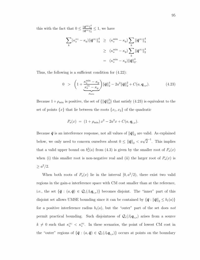
95

this with the fact that 0 ≤ ‖q(k)‖44

‖q(k)‖42

≤ 1, we have

∑

k

(κ(k)

s − κg)‖q(k)‖44 ≥ (κmin

s − κg)∑

k

‖q(k)‖44

≥ (κmins − κg)

∑

k

‖q(k)‖42

= (κmins − κg)‖q‖4

2.

Thus, the following is a sufficient condition for (4.22):

0 >

(

1 +κmin

s − κg

κ(0)s − κg

︸ ︷︷ ︸

ρmin

)

‖q‖42 − 2a2‖q‖2

2 + C(a, qr,ν). (4.23)

Because 1+ρmin is positive, the set of {‖q‖22} that satisfy (4.23) is equivalent to the

set of points {x} that lie between the roots {x1, x2} of the quadratic

Pa(x) = (1 + ρmin) x2 − 2a2x+ C(a, qr,ν).

Because q is an interference response, not all values of ‖q‖2 are valid. As explained

below, we only need to concern ourselves about 0 ≤ ‖q‖2 < a√

2−1

. This implies

that a valid upper bound on b2∗(a) from (4.3) is given by the smaller root of Pa(x)

when (i) this smaller root is non-negative real and (ii) the larger root of Pa(x) is

≥ a2/2.

When both roots of Pa(x) lie in the interval [0, a2/2), there exist two valid

regions in the gain-a interference space with CM cost smaller than at the reference,

i.e., the set {q : (a, q) ∈ Qc(βrqr,ν)} becomes disjoint. The “inner” part of this

disjoint set allows UMSE bounding since it can be contained by {q : ‖q‖2 ≤ b1(a)}

for a positive interference radius b1(a), but the “outer” part of the set does not

permit practical bounding. Such disjointness of Qc(βrqr,ν) arises from a source

k 6= 0 such that κ(k)s < κ(0)

s . In these scenarios, the point of lowest CM cost in

the “outer” regions of {q : (a, q) ∈ Qc(βrqr,ν)} occurs at points on the boundary

96

of Q(0)ν of the form q = (. . . , 0, 0, aejθ

√2−1, 0, 0, . . . )t and hence with ‖q‖2

2 = a2/2.

Thus, when x2 ≥ a2/2, we can be assured that all valid interference responses (i.e.,

{q : (a, q) ∈ Q(0)ν }) with CM cost less than the reference can be bounded by some

radius b1.

Solving for the roots of Pa(x) yields (with the convention x1 ≤ x2)

{x1, x2} =a2 ±

√

a4 − (ρmin + 1)C(a, qr,ν)

ρmin + 1

= a2

1 ±

√

1 − (ρmin + 1)C(a,qr,ν)

a4

ρmin + 1

,

and both roots are non-negative real when 0 ≤ C(a, qr,ν)/a4 ≤ (ρmin + 1)−1. It can

be shown that x2 > a2/2 occurs when C(a, qr,ν)/a4 ≤ (3 − ρmin)/4. Since ρmin ≥ 1

implies (3 − ρmin)/4 ≤ (ρmin + 1)−1, both root requirements are satisfied when

0 ≤ C(a, qr,ν)

a4≤ 3 − ρmin

4. (4.24)

4.A.4 Proof of Theorem 4.1

In this section we use the expression for b∗(a) from (4.7) and a suitably chosen

reference response qr,ν ∈ Qa ∩ Q(0)ν to upper bound Ju,ν(qc,ν). Plugging (4.7) in

(4.4),

Ju,ν(qc,ν)

σ2s

≤ maxa

1 −√

1 − (ρmin + 1)C(a,qr,ν)

a4

ρmin +

√

1 − (ρmin + 1)C(a,qr,ν)

a4

(4.25)

when 0 ≤ C(a, qr,ν)

a4≤ 3 − ρmin

4.

Note that the fraction on the right of (4.25) is non-negative and strictly increasing in

C(a, qr,ν)/a4 over the valid range of C(a, qr,ν)/a

4. Hence, finding a that maximizes

this expression can be accomplished by finding a that maximizes C(a, qr,ν)/a4. To

97

find these maxima, we first rewrite C(a, qr,ν)/a4 from (4.22):

C(a, qr,ν)

a4= C1

(

1

2(a2)−2 − κyr

(γ

σ2s

)−1

(a2)−1 + C2

)

,

where C1 and C2 are independent of a. Computing the partial derivative with

respect to the quantity a2,

∂

∂(a2)

{C(a, qr,ν)

a4

}

= C1 (a2)−3

(

κyr

(γ

σ2s

)−1

a2 − 1

)

.

Setting the partial derivative to zero yields the unique finite maximum

a2max =

(γ

σ2s

)

κyr .

Plugging a2max into (4.22) gives the simple result

C(amax, qr,ν)

a4max

=κ(0)

s − κyr

κ(0)s − κg

= 1 − κg − κyr

κg − κ(0)s,

and the C(a, qr,ν)/a4 requirement (4.24) translates into

1 + ρmin

4≤ κg − κyr

κg − κ(0)s

≤ 1. (4.26)

Finally, plugging C(amax, qr,ν)/a4max into (4.25) gives

Ju,ν(qc,ν)

σ2s

≤1 −

√

(1 + ρmin)κg−κyr

κg−κ(0)s

− ρmin

ρmin +√

(1 + ρmin)κg−κyr

κg−κ(0)s

− ρmin

. (4.27)

We now establish the existence of an attainable CM-minimizing global response

associated with the desired user at delay ν, i.e., qc,ν ∈ Qa ∩ Q(0)ν . For simplicity,

we assume that the space q is finite dimensional. We will exploit the Weierstrass

theorem [Luenberger Book 69, p. 40], which says that a continuous cost functional

has a local minimum in a compact set if there exist points in the interior of the set

which give cost lower than anywhere on the boundary.

98

By definition, all points in Qc(βrqr,ν) have CM cost less than or equal to Jc(yr),

the CM cost everywhere on the boundary of Qc(βrqr,ν). To make this inequality

strict, we expand Qc(βrqr,ν) to form the new set Q′c(βrqr,ν), defined in terms of

boundary cost Jc(yr) + ε (for arbitrarily small ε > 0). Thus, all points on the

boundary of Q′c(βrqr,ν) will have CM cost strictly greater than Jc(yr). But how do

we know that such a set Q′c(βrqr,ν) exists? We simply need to reformulate (4.22)

with ε-larger Jc(yr), resulting in ε-larger C(a, qr,ν) and a modified quadratic Pa(x)

in sufficient condition (4.23). As long as the new roots (call them x′1 and x′2) satisfy

x′1 ∈ [0, a2/2) and x′2 > a2/2, the set {q : (a, q) ∈ Q′c(βrqr,ν)} is well defined, and

as long as this holds for the worst-case a (i.e., amax), Q′c(βrqr,ν) will itself be well

defined. This behavior can be guaranteed, for arbitrarily small ε, by replacing (4.26)

with the stricter condition

1 + ρmin

4<

κg − κyr

κg − κ(0)s

≤ 1. (4.28)

To summarize, (4.28) guarantees the existence of a closed and bounded set Q′c(βrqr,ν)

containing an interior point βrqr,ν with CM cost strictly smaller than all points on

the set boundary.

Due to attainibility requirements, our local minimum search must be constrained

to the relative interior of the Qa manifold (which has been embedded in a possibly

higher-dimensional q-space). Can we apply the Weierstrass theorem on this man-

ifold? First, we know the Qa manifold intersects Q′c(βrqr,ν), namely at the point

βrqr,ν . Second, we know that the relative boundary of the Qa manifold occurs out-

side Q′c(βrqr,ν), namely at infinity. These two observations imply that the boundary

of Qa ∩ Q′c(βrqr,ν) relative to Qa must be a subset of the boundary of Q′

c(βrqr,ν).

Hence, the interior of Qa ∩Q′c(βrqr,ν) relative to Qa contains points which give kur-

tosis strictly higher than those on the boundary of Qa ∩ Q′c(βrqr,ν) relative to Qa.

99

Finally, the domain (i.e., Qa ∩ Q′c(βrqr,ν) relative to Qa) is closed and bounded,

hence compact. Thus the Weierstrass theorem ensures the existence of a local CM

minimum in the interior of Qa ∩ Q′c(βrqr,ν) relative to Qa under (4.28). Recalling

that Q′c(βrqr,ν) ⊂ Q(0)

ν , we see that there exists an attainable locally CM-minimizing

response associated with the desired user at delay ν.

Theorem 4.1 follows directly from (4.27) with reference choice qr,ν = qm,ν ∈

Qa ∩ Q(0)ν . Note that we restrict ourselves to qm,ν ∈ Q(0)

ν , which may not always be

the case.

4.A.5 Proof of Theorem 4.2

In this section we find an upper bound for Ju,ν(qc,ν) that involves the UMSE of

reference estimators, Ju,ν(qr,ν), rather than the kurtosis of reference estimates, κyr.

The choosing the reference to be the MMSE estimator can be considered a special

case. The conditions we establish below will guarantee that qm,ν ∈ Q(0)ν .

We will take advantage of the fact that Ju,ν

∣∣max,κyr

c,νin (4.27) is a strictly decreasing

function of κg−κyr

κg−κ(0)s

over its valid range. From (4.19),

κg − κy

κg − κ(0)s

=

∑

k(κg − κ(k)s )‖q(k)‖4

4

(κg − κ(0)s )‖q‖4

2

=(κg − κ(0)

s )|q(0)ν |4 +

∑

k(κg − κ(k)s )‖q(k)‖4

4

(κg − κ(0)s )‖q‖4

2

.

Examining the previous equation, 0 ≤ ‖q‖44

‖q‖42

≤ 1 implies that

∑

k

(κg − κ(k)

s )‖q(k)‖44 ≥ (κg − κmax

s )‖q‖44 ≥

0, κmaxs ≤ κg

(κg − κmaxs )‖q‖4

2, κmaxs > κg

(4.29)

and

∑

k

(κg − κ(k)

s )‖q(k)‖44 ≤ (κg − κmin

s )‖q‖44 ≤ (κg − κmin

s )‖q‖42. (4.30)

100

Note that in (4.30) and the super-Gaussian case of (4.29), equality is reached by

global responses of the form q = αe(k)

i , where k corresponds to the source with

minimum and maximum kurtosis, respectively.

Considering first the sub-Gaussian interference case (κmaxs ≤ κg), we claim

κg − κy

κg − κ(0)s

≥ |q(0)ν |4

‖q‖42

=

(

1 +Ju,ν(q)

σ2s

)−2

(4.31)

since the definition of Ju,ν(q) in (2.31) implies

‖q‖42 =

(|q(0)

ν |2 + ‖q‖22

)2= |q(0)

ν |4(

1 +‖q‖2

2

|q(0)ν |2

)2

= |q(0)

ν |4(

1 +Ju,ν(q)

σ2s

)2

.

Applying (4.31) to (4.27), we obtain

Ju,ν

∣∣max,κyr

c,ν

σ2s

≤1 −

√

(1 + ρmin)(

1 +Ju,ν(qr,ν)

σ2s

)−2

− ρmin

ρmin +

√

(1 + ρmin)(

1 +Ju,ν(qr,ν)

σ2s

)−2

− ρmin

when (4.28) is satisfied. Inequality (4.31) implies that

1 + ρmin

4<

(

1 +Ju,ν(qr,ν)

σ2s

)−2

⇔ Ju,ν(qr,ν)

σ2s

< −1 +2√

ρmin + 1

is sufficient for the left inequality of (4.28). Turning our attention to the right

inequality of (4.28), we can use (4.30) to say

κg − κy

κg − κ(0)s

≤ |q(0)ν |4

‖q‖42

+ ρmin‖q‖4

2

‖q‖42

=

(

1 +Ju,ν(q)

σ2s

)−2(

1 + ρmin

J2u,ν(q)

σ4s

)

(4.32)

since (2.31) implies

‖q‖42

‖q‖42

=

(

‖q‖22 + |q(0)

ν |2‖q‖2

2

)−2

=

(

1 +σ2

s

Ju,ν(q)

)−2

=J2

u,ν(q)

σ4s

(

1 +Ju,ν(q)

σ2s

)−2

.

Then, inequality (4.32) implies that a sufficient condition for the right side of equa-

tion (4.28) is

(

1 +Ju,ν(qr,ν)

σ2s

)−2(

1 + ρmin

J2u,ν(qr,ν)

σ4s

)

≤ 1 ⇔ Ju,ν(qr,ν)

σ2s

≤ 2

ρmin − 1.

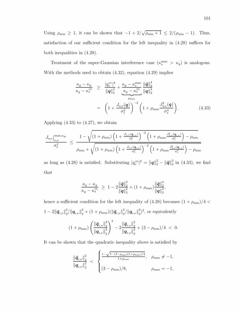
101

Using ρmin ≥ 1, it can be shown that −1 + 2/√ρmin + 1 ≤ 2/(ρmin − 1). Thus,

satisfaction of our sufficient condition for the left inequality in (4.28) suffices for

both inequalities in (4.28).

Treatment of the super-Gaussian interference case (κmaxs > κg) is analogous.

With the methods used to obtain (4.32), equation (4.29) implies

κg − κy

κg − κ(0)s

≥ |q(0)ν |4

‖q‖42

+κg − κmax

s

κg − κ(0)s

︸ ︷︷ ︸

ρmax

‖q‖42

‖q‖42

=

(

1 +Ju,ν(q)

σ2s

)−2(

1 + ρmax

J2u,ν(q)

σ4s

)

. (4.33)

Applying (4.33) to (4.27), we obtain

Ju,ν

∣∣max,κyr

c,ν

σ2s

≤1 −

√

(1 + ρmin)(

1 +Ju,ν(qr,ν)

σ2s

)−2 (

1 + ρmaxJ2u,ν(qr,ν)

σ4s

)

− ρmin

ρmin +

√

(1 + ρmin)(

1 +Ju,ν(qr,ν)

σ2s

)−2 (

1 + ρmaxJ2u,ν(qr,ν)

σ4s

)

− ρmin

as long as (4.28) is satisfied. Substituting |q(0)ν |2 = ‖q‖2

2 − ‖q‖22 in (4.33), we find

that

κg − κy

κg − κ(0)s

≥ 1 − 2‖q‖2

2

‖q‖22

+ (1 + ρmax)‖q‖4

2

‖q‖42

,

hence a sufficient condition for the left inequality of (4.28) becomes (1 + ρmin)/4 <

1 − 2‖qr,ν‖2

2/‖qr,ν‖2

2+ (1 + ρmax)(‖qr,ν‖2

2/‖qr,ν‖2

2)2, or equivalently

(1 + ρmax)

(

‖qr,ν‖2

2

‖qr,ν‖2

2

)2

− 2‖qr,ν‖2

2

‖qr,ν‖2

2

+ (3 − ρmin)/4 < 0.

It can be shown that the quadratic inequality above is satisfied by

‖qr,ν‖2

2

‖qr,ν‖2

2

<

1−√

1−(3−ρmin)(1+ρmax)/4

1+ρmax, ρmax 6= −1,

(3 − ρmin)/8, ρmax = −1,

102

and since Ju,ν(q) =(‖q‖2

2/‖q‖22

)/(1−‖q‖2

2/‖q‖22

)is strictly increasing in ‖q‖2

2‖q‖22,

the following must be sufficient for the left inequality of (4.28).

Ju,ν(qr,ν)

σ2s

<

1−√

1−(3−ρmin)(1+ρmax)/4

ρmax+√

1−(3−ρmin)(1+ρmax)/4, ρmax 6= −1,

3−ρmin

5+ρmin, ρmax = −1.

(4.34)

As for the right inequality of (4.28), it can be shown that the quantities in (4.34) are

smaller than 2/(ρmin − 1). Thus, satisfaction of (4.34) suffices for both inequalities

in (4.28).

4.A.6 Proof of Theorem 4.3

Here, we reformulate the upper bound (4.11). To simplify the presentation of the

proof, the shorthand notation J := Ju,ν(qm,ν)/σ2s will be used.

Starting with the non-super-Gaussian case (i.e., κmaxs ≤ κg), (4.11) says

Ju,ν

∣∣max,Ju,ν(qm,ν)

c,ν

σ2s

=1 −

√

(1 + ρmin)(1 + J)−2 − ρmin

ρmin +√

(1 + ρmin)(1 + J)−2 − ρmin

,

from which routine manipulations yield

Ju,ν

∣∣max,Ju,ν(qm,ν)

c,ν

σ2s

=1 −

√

1 −((ρmin − 1) + ρmin(2J + J2)

)(2J + J2)

(ρmin − 1) + ρmin(2J + J2).

For x ∈ R such that |x| < 1, the binomial series [Rudin Book 76] may be used to

claim

√1 − x = 1 − x

2− x2

8−O(x3).

Applying the previous expression with x =((ρmin − 1) + ρmin(2J + J2)

)(2J + J2),

103

we find that

Ju,ν

∣∣max,Ju,ν(qm,ν)

c,ν

σ2s

=1

2

((ρmin − 1) + ρmin(2J + J2)

)(2J + J2)

(ρmin − 1) + ρmin(2J + J2)

+1

8

((ρmin − 1) + ρmin(2J + J2)

)2(2J + J2)2

(ρmin − 1) + ρmin(2J + J2)+ O(J3)

= J +ρmin

2J2 + O(J3).

Finally, subtraction of J gives the first case in (4.12).

For the super-Gaussian case (i.e., κmaxs > κg), (4.11) says

Ju,ν

∣∣max,Ju,ν(qm,ν)

c,ν

σ2s

=1 −

√

(1 + ρmin)(1 + J)−2(1 + ρmaxJ2) − ρmin

ρmin +√

(1 + ρmin)(1 + J)−2(1 + ρmaxJ2) − ρmin

,

from which routine manipulations yield

Ju,ν

∣∣max,Ju,ν(qm,ν)

c,ν

σ2s

=

ρmaxJ2 + 1 −

√

1 + (2−2ρmax)J + (1+ρmax+ρminρmax−5ρmin)J2 + O(J3)

(ρmin − 1) + 2ρminJ + (ρmin − ρmax)J2.

As before, we use the binomial series expansion for√

1 − x, but now with x =

(2ρmax −2)J +(5ρmin−1−ρmax −ρminρmax)J2 +O(J3). After some algebra, we find

Ju,ν

∣∣max,Ju,ν(qm,ν)

c,ν

σ2s

= J +1

2

(ρmin − ρmax)(ρmin − 1)J2 + O(J3)

(ρmin − 1) + 2ρminJ + (ρmin − ρmax)J2

Finally we apply the series approximation

1

1 − y= 1 + y + O(y2)

with y = −(2ρminJ + (ρmin − ρmax)J2)/(ρmin − 1) for ρmin 6= 1. Straightforward

algebra yields

Ju,ν

∣∣max,Ju,ν(qm,ν)

c,ν

σ2s

= J +1

2(ρmin − ρmax)J

2 + O(J3).

Taking the limit ρmin → 1, it is evident that no problems arise at the point ρmin = 1.

Subtraction of J from the last statement gives the second case in (4.12).

Chapter 5

Sufficient Conditions for the Local

Convergence of CM Algorithms1

5.1 Introduction

Perhaps the greatest challenge facing successful application of the CM criterion in

arbitrary interference environments results from the difficulty in determining CM-

minimizing estimates of the desired source (as opposed to mistakenly estimating an

interferer). The potential for “interference capture” is a direct consequence of the

fact that the CM criterion exhibits multiple local minima in the estimator parameter

space, each corresponding to a CM estimator of a particular source at a particular

delay. Such multi-modality might be suspected from (2.35); the CM criterion is

based on a particular property of the estimates {yn}, and one can imagine a case

in which this property is satisfied to a similar extent by, e.g., {yn} ≈ {s(0)n } and

{yn} ≈ {s(1)n } when {s(0)

n } and {s(1)n } have the same statistics.

Various “multiuser” modifications of the CM criterion have been proposed to

1The main results of this chapter also appear in the manuscript [Schniter TSP 00].

104

105

jointly estimate all sub-Gaussian sources present in a multi-source environment.

Some of these techniques add a non-negative term to the CM criterion which penal-

izes correlation between any pair of L parallel estimator outputs, forcing the L esti-

mators to generate estimates of distinct sources [Batra GLOBE 95],

[Papadias SPL 96], [Touzni ICASSP 98]. Other techniques use the CM criterion in

a successive interference cancellation scheme, whereby estimates of the n strongest

sub-Gaussian sources are used to remove their respective contributions to the re-

ceived signal before estimation of the n+1th source [Treichler TASSP 85b]. Both

of these approaches, however, require knowledge of the number of (non-Gaussian)

sources, result in significant increase in computational complexity when the number

of sources is large, and generate estimates with questionable MSE performance. In-

stead, we focus on the well-known standard CM (or “Godard” [Godard TCOM 80])

criterion and consider desired-source convergence as an outcome of proper initial-

ization.

Closed-form expressions for CM estimators do not generally exist, and thus gradi-

ent descent (GD) methods provide the typical means of solving for these estimators.

Because exact gradient descent requires statistical knowledge of the received process

that is not usually available in practical situations, stochastic GD algorithms such

as CMA are used to estimate and track the (possibly time-varying) CM estimator.

It is widely accepted, however, that small step-size stochastic GD algorithms exhibit

mean transient and steady-state behaviors very close to those of exact GD under

typical operating conditions [Benveniste Book 90], [Ljung Book 99]. Hence, we cir-

cumvent the details of stochastic adaptation by restricting our attention to (exact)

GD minimization of the CM cost. An important property of GD minimization is

that the location of algorithm initialization completely determines the stationary

106

point to which the GD trajectory will eventually converge. The description of the

CM-GD regions-of-convergence (ROC) in terms of estimator parameters appears to

be a very difficult problem, however, and attempts at finding closed-form expres-

sions for the ROC boundaries have thus far been unsuccessful [Chung Thesis 99],

[Gu TSP 99].

In this chapter, we derive three sufficient conditions under which CM-GD min-

imization will generate an estimator for the desired source. The conditions are

expressed in terms of statistical properties of the initial estimates, specifically, CM

cost, kurtosis, and signal to interference-plus-noise ratio (SINR). Earlier attempts

at describing the interference capture or “local convergence” properties of CMA

have been made by Treichler and Larimore in [Treichler TASSP 85a] and Li and

Ding in [Li TSP 95]. Treichler and Larimore constructed a simplifying approxima-

tion to the mean behavior of CMA for the case of a constant envelope signal in

tonal interference and inferred the roles of initial signal-to-interference ratio and

initial estimator parameterization on desired convergence. Li and Ding derived a

sufficient kurtosis condition for the local convergence of the Shalvi-Weinstein (SW)

algorithm [Shalvi TIT 90] and suggested that the condition applies to small-stepsize

CMA as well. Our analysis and simulations suggest that the local convergence be-

havior of CMA differs from that of the SW algorithm, contrasting certain claims of

[Li TSP 95].

The organization of the chapter is as follows. Section 5.2 derives initialization

conditions sufficient for CM-GD convergence to desired source estimates, Section 5.3

discusses the implications of these conditions on choice of CM-GD initialization

scheme, Section 5.4 presents numerical simulations verifying our analyses, and Sec-

tion 5.5 concludes the chapter.

107

5.2 Sufficient Conditions for Local Convergence

of CM-GD

5.2.1 The Main Idea

The set of global responses associated with the desired source (k = 0) at estimation

delay ν will be denoted Q(0)ν and defined as follows.

Q(0)

ν :=

{

q s.t. |q(0)

ν | > max(k,δ)6=(0,ν)

|q(k)

δ |}

. (5.1)

Note that under S1)–S3), the previous definition associates an estimator with a

particular {source, delay} combination if and only if that {source, delay} contributes

more energy to the estimate than any other {source, delay}. Choosing, as a reference

set, the global responses on the boundary of Q(0)ν with minimum CM cost,

{qr} := arg minq∈bndr(Q(0)

ν )

Jc(q), (5.2)

we will denote the set of all global responses in Q(0)ν with CM cost no higher than

Jc(qr) by

Qc(qr) :={q s.t. Jc(q) ≤ Jc(qr)

}∩Q(0)

ν .

The main idea is this. Since all points in a CM gradient descent (CM-GD) trajectory

have CM cost less than or equal to the cost at initialization, a CM-GD trajectory

initialized within Qc(qr) must be entirely contained in Qc(qr) and thus in Q(0)ν . In

other words, when a particular response q yields sufficiently small CM cost, CM-

GD initialized from q will preserve the {source, delay} combination associated with

q. Note that initializing within Qc(qr) is sufficient, but not necessary, for eventual

CM-GD convergence to a stationary point in Q(0)ν .

108

Since the size and shape of Qc(qr) are not easily characterizable, we find it more

useful to derive sufficient CM-GD initialization conditions in terms of well-known

statistical quantities such as kurtosis and SINR. It was shown in Section 2.5 that

CM cost and kurtosis are closely related, and we shall see that translation between

these two quantities is relatively straightforward. Translation of the initial CM-cost

condition into an initial SINR condition is more difficult but can be accomplished

through definition of SINRmin,ν , the SINR above which all q have scaled versions in

Qc(qr):

SINRmin,ν := min x s.t.

{

∀q : SINRν(q) ≥ x, ∃ a∗ s.t.a∗q

‖q‖2

∈ Qc(qr)

}

. (5.3)

If initializations in the set {q : SINRν(q) ≥ SINRmin,ν} are scaled so that they

lie within Qc(qr), the resulting CM-GD trajectories will remain within Qc(qr) and

hence within Q(0)ν . In other words, when a particular response q yields sufficiently

high SINR, CM-GD initialized from a properly scaled version of q will preserve

the source/delay combination associated with q. This sufficient SINR property is

formalized below.

Since Qc(qr) and SINRν(q) are all invariant to phase rotation (i.e., scalar mul-

tiplication by ejφ for φ ∈ R) of qr and q, respectively, we can (w.l.o.g.) restrict our

attention to the “de-rotated” set of global responses {q s.t. q(0)ν ∈ R+}. Such q allow

parameterization in terms of gain a = ‖q‖2 and interference response q (defined in

Section 2.3.3) where ‖q‖2 ≤ a. In terms of the pair (a, q), the SINR (2.32) can be

written

SINRν(a, q) =a2 − ‖q‖2

2

‖q‖22

,

109

so that (5.3) becomes

SINRmin,ν := min x

s.t.

{

∀(a, q) :a2 − ‖q‖2

2

‖q‖22

≥ x, ∃ a∗ s.t. (a∗,a∗

aq) ∈ Qc(qr)

}

. (5.4)

Under particular conditions on a and qr (made explicit in Section 5.2.2), there

exists a maximum interference gain b, specified as a function of system gain a, below

which all q are contained in Qc(qr):

bmax(a) := max b(a) s.t.{

∀ q : ‖q‖2 ≤ b(a), (a, q) ∈ Qc(qr)}

. (5.5)

For an illustration of a, bmax(a), and Qc(qr), see Fig. 5.1. Now, consider the quantity

SINRν(a, bmax) :=a2 − b2max(a)

b2max(a).

Note that SINR(a, bmax) = cot2(θ) for the θ in Fig. 5.1. Since SINRν(a, bmax) is a

decreasing function of bmax(a) (over its valid domain), definition (5.5) implies that

a2 − ‖q‖22

‖q‖22

≥ SINRν(a, bmax) ⇒ (a, q) ∈ Qc(qr).

Using the previous expression to minimize SINR in accordance with (5.4) yields the

key quantities defined in (5.3):

SINRmin,ν = mina

SINRν(a, bmax) (5.6)

a∗ = arg mina

SINRν(a, bmax). (5.7)

To summarize, when SINRν(q) ≥ SINRmin,ν and ‖q‖2 = a∗, CM-GD initialized from

q will preserve the {source, delay} combination associated with q.

5.2.2 Derivation of Sufficient Conditions

In this section we formalize the previously-described initialization conditions for CM-

GD local convergence. The main steps in the derivation are presented as theorems

and lemmas, with proofs appearing in Appendix 5.A.

110

q(0)ν

q

bmax(a)

a

θ

Qc(qr)

Figure 5.1: Illustration of maximum interference gain bmax(a) below which all global

responses with gain a are contained in the CM cost region Qc(qr).

Before presentation of the results, we introduce the following notation that is

specific to this chapter.

κimins :=

min0≤k≤K κ(k)s , dim(q(0)) > 1

min1≤k≤K κ(k)s , dim(q(0)) = 1

(5.8)

ρimin :=κg − κimin

s

κg − κ(0)s, (5.9)

σ2y

∣∣crit

:= γ

(4

κ(0)s + κimin

s + 2κg

)

. (5.10)

Above, “dim” denotes the dimension of a vector. Note that the second case in (5.8)

applies only when the desired source contributes zero intersymbol interference (ISI).

Thus, κimins equals κmin

s in most cases.

Lemma 5.1. The minimum CM cost on the boundary of Q(0)ν is

Jc(qr) = minq∈bndr(Q(0)

ν )

Jc(q) = γ2

(

1 − 4

κ(0)s + κimin

s + 2κg

)

. (5.11)

111

Theorem 5.1. If {yn} are initial estimates of the desired source at delay ν (i.e.,

yn = qtinits(n) for qinit ∈ Q(0)

ν ∩Qa) with CM cost

Jc(yn) < γ2

(

1 − 4

κ(0)s + κimin

s + 2κg

)

, (5.12)

then estimators resulting from subsequent CM-minimizing gradient descent will also

yield estimates of the desired source at delay ν.

Theorem 5.2. If {yn} are initial estimates of the desired source at delay ν (i.e.,

yn = qtinits(n) for qinit ∈ Q(0)

ν ∩ Qa) with variance σ2y = σ2

y

∣∣crit

and normalized

kurtosis

κy < κcrity :=

1

4

(κ(0)

s + κimins + 2κg

), (5.13)

then estimators resulting from subsequent CM-minimizing gradient descent will also

yield estimates of the desired source at delay ν.

Theorem 5.3. If κ(0)s ≤ (κimin

s + 2κg)/3, and if {yn} are initial estimates with

variance σ2y = σ2

y

∣∣crit

and SINRν(yn) > SINRmin,ν, where

SINRmin,ν =

√1+ρimin

2−√1+ρimin

, κmaxs ≤ κg,

ρmax+√

1−(1+ρmax)(3−ρimin)/4

1−√

1−(1+ρmax)(3−ρimin)/4, ρmax 6= −1

5+ρimin

3−ρimin, ρmax = −1

, κmaxs > κg,

(5.14)

then estimators resulting from subsequent CM-minimizing gradient descent will also

yield estimates of the desired source at delay ν.

We now make a few comments on the theorems. First, notice the presence of gain

condition σ2y = σ2

y

∣∣crit

in Theorems 5.2 and 5.3. One might wonder how necessary this

gain condition is, and our answer is twofold. As we have derived sufficient conditions

112

for convergence, none are strictly necessary. But it is possible to construct scenarios

where satisfaction of all except the gain condition results in misconvergence. The

existence of such scenarios implies that initial kurtosis cannot be the sole indicator

of CM-GD convergence, as suggested in [Li TSP 95]. Fortunately, it appears that

such scenarios are quite rare unless σ2y is far from σ2

y

∣∣crit

or unless the SINR and/or

kurtosis conditions are themselves near violation. Thus, in practice, successful CM-

GD convergence should be quite robust to small violations of σ2y = σ2

y

∣∣crit

.

Finally, it should be pointed out that the relatively complicated expressions in

Theorem 5.3 simplify under the operating conditions commonly encountered in, e.g.,

data communication. When the sources of interference are non-super-Gaussian (i.e.,

κmaxs ≤ κg) and none have kurtosis less than the desired source (i.e., κ(0)

s ≤ κ(k)s ), we

find that ρmin = 1, and thus SINRmin,ν = 1 +√

2 or 3.8 dB.

5.3 Implications for CM Initialization Schemes

In the previous section we have shown that there exist statistical properties of initial

estimates which guarantee that subsequent CM gradient descent will produce an

estimator of the same source at the same delay. In this section we suggest how one

might satisfy these initialization conditions.

We consider CM initialization procedures capable of being described by the fol-

lowing two-step procedure: 1) design of one or more initialization hypotheses, 2)

choice among hypotheses. Note that most popular CM initialization procedures,

such as the single-spike scheme discussed below, fall within this general framework.

In evaluating a CM-GD initialization scheme, we must then consider the diffi-

culty in both the design and evaluation of initialization hypotheses. The theorems

in the previous section suggest that when a particular source or delay is desired,

113

initialization hypotheses should be designed to either (i) maximize SINR, or (ii)

minimize CM cost or kurtosis when the initial estimates are known to correspond to

a desired source/delay combination.

5.3.1 The “Single-Spike” Initialization

The so-called single-spike initialization, first proposed in [Godard TCOM 80], is

quite popular in single-user environments. Single-spike initializations for single-

sensor baud-spaced equalizers (i.e., P = 1) are characterized by impulse responses

with a single nonzero coefficient, i.e., f(z) = z−δ. There exists a straightforward

extension to multi-rate/multi-channel (i.e., P > 1) estimators: f(z) = 1z−δ for

1 := (√

1/P , . . . ,√

1/P )t ∈ RP . For P = 2, this has been called the “double-spike”

initialization [Johnson Chap 99]. The spike position is often an important design

parameter, as we explain below.

Since the spike method yields an initial global response equaling (a delayed

version of) the channel response, the kurtosis of the initial estimates can be expressed

directly in terms of the channel coefficients {h(k)

i }:

κy =∑

k

(κ(k)

s − κg)‖q(k)‖4

4

‖q‖42

+ κg =

∑

k,i |1th(k)

i |4(κ(k)s − κg)

(∑

k,i |1th(k)

i |2)2 + κg.

If we assume a single sub-Gaussian user in the presence of additive white Gaussian

noise (AWGN) of variance σ2w at each sensor, the previous expression simplifies to

κy = (κ(0)

s − κg)

∑

i |1th(0)

i |4(∑

i |1th(0)

i |2 + σ2w/σ

2s

)2 + κg. (5.15)

Table 5.1 shows initial kurtoses κy from (5.15) for Signal Processing Information

Base (SPIB) microwave channel models in AWGN (resulting in 20dB SNR at channel

output), along with the critical kurtosis κcrity from (5.13). From Table 5.1 we see

that the single-spike initialization procedure generates estimates with kurtosis less

114

Table 5.1: Single-spike kurtoses for SPIB microwave channel models and 20 dB

SNR.

Channel # 1 2 3 4 5 6 7 8 9 κcrity

BPSK 1.17 1.17 1.41 1.98 1.94 1.76 1.16 1.69 1.70 2

8-PAM 1.87 1.86 2.02 2.37 2.34 2.23 1.86 2.19 2.19 2.38

QPSK 1.09 1.15 1.26 1.49 1.47 1.38 1.24 1.35 1.35 1.5

64-QAM 1.43 1.48 1.53 1.68 1.67 1.62 1.53 1.60 1.60 1.69

than the critical value for all SPIB channels. The implication is that CM gradient

descent from a single-spike initialization with magnitude chosen in accordance with

Theorem 5.2 typically preserves the estimation delay of the initial estimates. Similar

conjectures have been made in [Li TSP 95] and [Johnson Chap 99].

Since MMSE performance is known to vary (significantly) with estimation delay,

the connection between Wiener and CM performance established in Chapter 4 im-

plies that the MSE performance of CM-minimizing estimates should also vary with

estimation delay. Thus, from our observations on the local convergence of single-

spike initializations, we conclude that the asymptotic MSE performance CM-GD

estimates can be directly linked to the choice of initial spike delay.

5.3.2 Initialization Using Partial Information

Though the single-spike scheme has desirable properties in (noisy) single-user ap-

plications, one would not expect it to yield reliable estimates of the desired source

when in the presence of significant sub-Gaussian interference since single-spike ini-

tialized CM-GD might lock onto a sub-Gaussian interferer instead of the desired

115

source. With partial knowledge of the desired user’s channel, however, it may be

possible to construct rough guesses of the desired estimator that are good enough

for use as CM-GD initializations. Then, if the initialization satisfies the sufficient

conditions in the previous section, we know that CM-GD can be used to design an

an estimator with nearly optimal MSE performance (as discussed in Section 2.5).

The “partial knowledge” may come in various forms, for example, short training

records in semi-blind equalization applications, rough direction-of-arrival knowledge

in array applications, spreading sequences in code-division multiple access (CDMA)

applications, or desired polarization angle in cross-pole interference cancellation.

We have seen that various criteria could be used to design and evaluate initializa-

tion hypotheses. Since reliable evaluation of higher-order statistics typically require

a larger sample size than second-order statistics, the design and/or evaluation of

SINR-based initializations might be advantageous when sample size is an issue. For

this reason, SINR-based methods will be considered for the remainder of this sec-

tion. Still, good results have been reported for kurtosis-based CM-GD initialization

schemes for CDMA applications when sample size is not an issue [Schniter ALL 98].

The SINR-maximizing linear estimator is given by Wiener estimator fm,ν(z). It

was shown in Appendix 2.A that

fm,ν(z) = z−νσ2s

(

E{r(z)rH( 1

z∗)})†

h(0)( 1z∗

) (5.16)

where (·)† denotes pseudo-inverse. As evident from (5.16), design of fm,ν(z) re-

quires knowledge of the desired channel h(0)(z) in addition to the auto-correlation

of the received signal. Though various methods exist for the design of blind SINR-

maximizing (i.e., MSE-minimizing) estimators based on partial knowledge of h(0)(z),

the Wiener expression (5.16) suggests the following CM initialization when given

116

only a channel estimate h(0)(z) and knowledge of E{r(z)rH(1/z∗)

}.

finit(z) = z−ν(

E{r(z)rH( 1

z∗)})†

h(0)( 1z∗

). (5.17)

Note that (5.17) may require additional scaling to satisfy the σ2y-requirements of

Theorems 5.2 and 5.3.

5.4 Numerical Examples

In Fig. 5.2, CM-GD minimization trajectories conducted in estimator space are

plotted in global (i.e. channel-plus-estimator) space (q ∈ R2) to demonstrate the

key results of this chapter. CM-GD can be described by the update equation f (n+

1) = f (n) − µ∇fJc, where f = (. . . , f t−1, f

t0, f

t1, . . . )

t is a vector containing the

estimator parameter coefficients, µ is a vanishingly small positive stepsize, and ∇f

denotes the gradient with respect to f . When the estimator is FIR we can write

q = (fHH)t, implying the global-response CM-GD update equation q(n+1) =

q(n) − µHt(∇fJc

)∗. In all experiments, we use a two-parameter estimator and a

FIR channel that corresponds to the following arbitrarily-chosen channel matrix H

(having condition number 3):

H =

0.2940 −0.0596

0.1987 0.9801

.

Fig. 5.2(a)-(c) depict the Q(0)ν boundaries as dash-dotted lines, the SINRmin,ν

boundaries as dashed lines, and the κcrity boundaries as dotted lines. Note that in

Fig. 5.2(a), the dash-dotted and dotted lines are coincident, while in Fig. 5.2(c),

the dash-dotted, dashed, and dotted lines are coincident. The three sub-plots in

Fig. 5.2 differ only in the kurtosis of the desired source: in Fig. 5.2(a) the sources

117

have κ(0)s = 1 and κ(1)

s = 1, in Fig. 5.2(b) κ(0)s = 2 and κ(1)

s = 1, while in Fig. 5.2(c)

κ(0)s = 2 and κ(1)

s = 4.

The following three behaviors can be observed in every sub-plot of Fig. 5.2.

First, all trajectories entering into Qc(qr) (denoted by the shaded region between

the dash-dotted lines) converge to an estimator for the desired source, confirming

Theorem 5.1. Next, all trajectories initialized with small enough kurtosis (indicated

by the region between the dotted lines) and proper gain (indicated by the fat shaded

arc) converge to an estimator for the desired source, thus confirming Theorem 5.2.

Finally, all trajectories initialized with high enough SINR (indicated by the region

between the dashed lines) and proper gain (again indicated by the fat shaded arc)

converge to estimators for the desired source, confirming Theorem 5.3.

Fig. 5.2 suggests that the sufficient-SINR condition of Theorem 5.3 is more re-

strictive than the sufficient-kurtosis condition of Theorem 5.2, which in turn is more

restrictive than the Jc-based condition of Theorem 5.1: the sufficient-SINR region

(between the dashed lines) is contained by the sufficient-kurtosis region (between

the dotted lines), which is contained by the sufficient-Jc region (between the dash-

dotted lines). The relative ordering of these three conditions is, in fact, formally

implied by the proofs in Appendix 5.A.

We stress again that initial kurtosis or SINR is not sufficient for desired local

convergence; initial estimator gain plays an important role. This is demonstrated

by Fig. 5.2(a)-(b) wherein some trajectories initialized within the SINRν(q) >

SINRmin,ν region (between the dashed lines), but with insufficient initial gain, con-

verge to the undesired equilibria q = (0,±1)t. Though recognized in

[Treichler TASSP 85a], this fact was overlooked in [Li TSP 95], resulting in some

overly strong claims about the convergence behavior of CMA.

118

−1.5 −1 −0.5 0 0.5 1 1.5

0

0.5

1

1.5

q1 (interference)

q 0 (de

sire

d)

(c)

−1.5 −1 −0.5 0 0.5 1 1.5

0

0.5

1

1.5

q1 (interference)

q 0 (de

sire

d)

(a)

−1.5 −1 −0.5 0 0.5 1 1.5

0

0.5

1

1.5

q1 (interference)

q 0 (de

sire

d)

(b)

Figure 5.2: CM-GD trajectories in channel-plus-estimator space (q ∈ R2) for (a)

κ(0)s = 1 and κ(1)

s = 1, (b) κ(0)s = 2 and κ(1)

s = 1, and (c) κ(0)s = 2 and κ(1)

s = 4.

Also shown are Q(0)ν boundaries (dash-dotted), SINRmin,ν boundaries (dashed), κcrit

y

boundaries (dotted), and Jc(q) < Jc(qr) regions (shaded). Fat shaded arcs denote

global responses giving σ2y = σ2

y

∣∣crit

. Notice that dotted and dash-dotted lines are

coincident in (a), while dotted, dash-dotted, and dashed lines are coincident in (c).

119

In Fig. 5.3 we examine probability of CM-GD convergence to desired {source,

delay} versus SINR for higher-dimensional estimators. CM gradient descents ran-

domly initialized in a ball around fm,ν (and subsequently normalized according to

Theorem 5.3) were conducted using random channel matrices {H} ∈ R10×11 with

zero-mean Gaussian elements. Every data point in Fig. 5.3 represents an average

of 500 CM-GD simulations. Fig. 5.3(a) demonstrates κ(0)s = 1 and ten interfering

sources with κ(k)s = 1; Fig. 5.3(b) demonstrates κ(0)

s = 2, five interfering sources with

κ(k)s = 1, and five interfering sources with κ(k)

s = 2; while Fig. 5.3(c) demonstrates

κ(0)s = 2, five interfering sources with κ(k)

s = 2, and five interfering sources with

κ(k)s = 4.

Fig. 5.3 also confirms the claim of Theorem 5.3: all properly-scaled CM-GD

initializations with SINRν greater than SINRmin,ν converge to the desired source.

Recalling that the SINR condition is sufficient, but not necessary, for desired con-

vergence, it is interesting to note that both Fig. 5.2 and Fig. 5.3 suggest that the

sufficiency of our SINR condition becomes “looser” as the kurtosis of the desired

source rises above the minimum interference kurtosis (i.e., as ρimin increases).

5.5 Conclusions

In this chapter we have derived, under the general linear model of Fig. 2.3, three

sufficient conditions for the convergence of CM-minimizing gradient descent to an

estimator for a particular source at a particular delay. The sufficient conditions are

expressed in terms of statistical properties of initial estimates, i.e., estimates gener-

ated by an estimator parameterization from which the gradient descent procedure

is initialized. More specifically, we have proven that when initial estimates result

in sufficiently low CM cost, or in sufficiently low kurtosis and a particular variance,

120

−20 −15 −10 −5 0 5 100

0.2

0.4

0.6

0.8

1

initial SINR

prob

abili

ty

(c)

−20 −15 −10 −5 0 5 100

0.2

0.4

0.6

0.8

1

initial SINR

prob

abili

ty

(b)

−20 −15 −10 −5 0 5 100

0.2

0.4

0.6

0.8

1

initial SINR

prob

abili

ty

(a)

Figure 5.3: Estimated probability of convergence to desired source/delay for random

channels and random initializations scaled according to Theorem 5.3 and plotted as

a function of initialization SINR. In (a) κ(0)s = 1 with interfering κ(k)

s ∈ {1, 3}, in

(b) κ(0)s = 2 with interfering κ(k)

s ∈ {1, 2}, and in (c) κ(0)s = 2 with interfering

κ(k)s ∈ {2, 4}. SINRmin,ν from (5.14) shown by dashed lines.

121

CM-GD will preserve the source/delay combination associated with the initial esti-

mator. In addition, we have proven that when the SINR of the initial estimates (with

respect to a particular source/delay combination) is above a prescribed threshold

and the estimates have a particular variance, CM-GD will converge to an estimator

of the same source/delay. These results suggest ways in which a priori channel

knowledge may be used to predict and control the convergence behavior of CMA

and are of particular importance in multi-user applications.

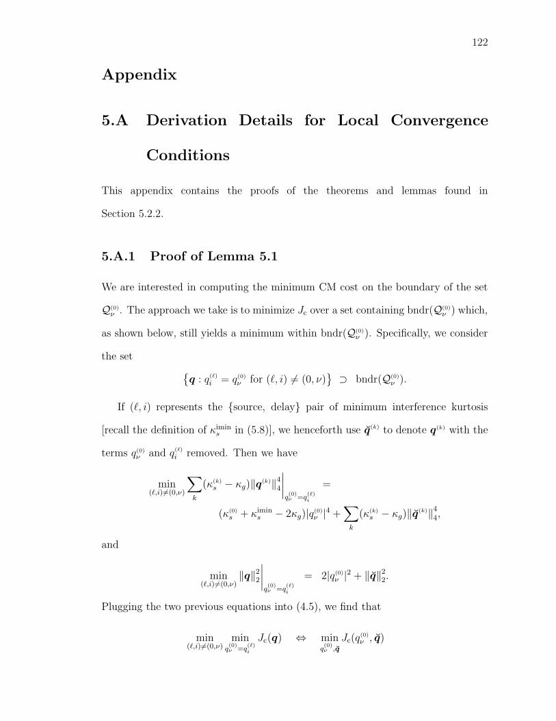
122

Appendix

5.A Derivation Details for Local Convergence

Conditions

This appendix contains the proofs of the theorems and lemmas found in

Section 5.2.2.

5.A.1 Proof of Lemma 5.1

We are interested in computing the minimum CM cost on the boundary of the set

Q(0)ν . The approach we take is to minimize Jc over a set containing bndr(Q(0)

ν ) which,

as shown below, still yields a minimum within bndr(Q(0)ν ). Specifically, we consider

the set

{q : q(`)

i = q(0)

ν for (`, i) 6= (0, ν)}

⊃ bndr(Q(0)

ν ).

If (`, i) represents the {source, delay} pair of minimum interference kurtosis

[recall the definition of κimins in (5.8)], we henceforth use q(k) to denote q(k) with the

terms q(0)ν and q(`)

i removed. Then we have

min(`,i)6=(0,ν)

∑

k

(κ(k)

s − κg)‖q(k)‖44

∣∣∣∣q(0)ν =q

(`)i

=

(κ(0)

s + κimins − 2κg)|q(0)

ν |4 +∑

k

(κ(k)

s − κg)‖q(k)‖44,

and

min(`,i)6=(0,ν)

‖q‖22

∣∣∣∣q(0)ν =q

(`)i

= 2|q(0)

ν |2 + ‖q‖22.

Plugging the two previous equations into (4.5), we find that

min(`,i)6=(0,ν)

minq(0)ν =q

(`)i

Jc(q) ⇔ minq(0)ν ,q

Jc(q(0)

ν , q)

123

where

Jc (q(0)ν , q)

σ4s

:= (κ(0)

s + κimins − 2κg)|q(0)

ν |4 +∑

k(κ(k)s − κg)‖q(k)‖4

4

+ κg

(2|q(0)

ν |2 + ‖q‖22

)2 − 2(γ/σ2s)(2|q(0)

ν |2 + ‖q‖22

)+ (γ/σ2

s)2

= (κ(0)

s + κimins + 2κg)|q(0)

ν |4 − 4((γ/σ2

s) − κg‖q‖22))|q(0)

ν |2 + Jc(q)/σ4s .

(5.18)

Zeroing the partial derivative of Jc (q(0)ν , q) w.r.t. |q(0)

ν |2 yields

arg min|q(0)

ν |2Jc (q(0)

ν , q) = 2(γ/σ2

s) − κg‖q‖22

κ(0)s + κimin

s + 2κg

, (5.19)

thus

Jc

(q(0)ν

∣∣min, q)

σ4s

=Jc(q)

σ4s

− 4κ2

g‖q‖42 − 2κg(γ/σ

2s)‖q‖2

2 + (γ/σ2s)

2

κ(0)s + κimin

s + 2κg

=∑

k

(κ(k)

s − κg)‖q(k)‖44 + κgd‖q‖4

2 − 2(γ/σ2s)d‖q‖2

2

+ (γ/σ2s )

2(1 − 4(κ(0)

s + κimins + 2κg)

−1)

(5.20)

using the abbreviation

d :=κ(0)

s + κimins − 2κg

κ(0)s + κimin

s + 2κg

. (5.21)

The gradient and Hessian analysis below reveals that, when κimins ≤ 2κg − κ(0)

s , the

(unique) global minimum of Jc

(q(0)ν

∣∣min, q)

occurs at q = 0, implying [via (5.20)]

that

minq∈bndr(Q(0)

ν )

Jc(q)

σ4s

= minq

Jc

(q(0)ν

∣∣min, q)

σ4s

=

(γ

σ2s

)2(

1 − 4

κ(0)s + κimin

s + 2κg

)

. (5.22)

Now for the gradient and Hessian analysis. For simplicity, we assume real-valued

quantities, though a similar technique may be used to establish the same result in the

124

complex-valued case. Using standard techniques (see, e.g., [Johnson IJACSP 95]),

it can be shown that the component of the gradient ∇qJc

(q(0)ν

∣∣min, q)

corresponding

to the direction of q(k)

i is

[

∇qJc

(q(0)

ν

∣∣min, q)](k)

i=((κ(k)

s − κg)|q(k)

i |2 + d(κg‖q‖2

2 − (γ/σ2s)))q(k)

i

and the component of the Hessian HqJc

(q(0)ν

∣∣min, q)

corresponding to the directions

of q(k)

i and q(`)

j is

[

HqJc

(q(0)

ν

∣∣min, q)](k,`)

i,j=

(3(κ(k)s − κg) + 2κgd) |q(k)

i |2 + d(κg‖q‖2

2 − (γ/σ2s )), k=` and i=j

2κgd · q(k)

i q(`)

j , else.

All q setting the gradient to zero are stationary points, but only those stationary

points with positive semi-definite (PSD) Hessians qualify as local minima.

From the previous expression, the stationary points are described by q with the

elements

q(k)

i =

0, or

±√

d((γ/σ2s )−κg‖q‖2

2)κ(k)s −κg

, when κ(k)s < κg and ‖q‖2

2 ≤ (γ/σ2s)/κg.

(5.23)

In stating the two conditions in (5.23), we have assumed κimins ≤ 2κg − κ(0)

s which

implies d ≤ 0. Noting that q(k)

i is independent of i, we can write ‖q‖22 =

∑

k Mk|q(k)

i |2

using the integer Mk to denote the number of nonzero q(k)

i in the candidate response.

Solving for ‖q‖22 and plugging it into (5.23) gives

q(k)

i = α(k)

i

√√√√d

(γ

σ2s

)(

1 + κgd∑

`

M`

κ(`)s − κg

)−11

κ(k)s − κg

for α(k)

i ∈ {−1, 0, 1},

when κ(k)s < κg and

∑

`M`

κ(`)s −κg

< 1κgd

(and where∑

i |α(k)

i | = Mk).

125

The Hessian will be PSD if and only if all of its principle minors are PSD. The

principle minors of HqJc

(q(0)ν

∣∣min, q)

take the form

d · γσ2

s

(

1 + κgd∑

`

M`

κ(`)s − κg

)−1

× · · ·

(

3+ 2κgd

κ(k)s −κg

)

α(k)2i − 1

2κg |d|α(k)i α

(`)j√

(κ(k)s −κg)(κ

(`)s −κg)

2κg|d|α(k)i α

(`)j√

(κ(k)s −κg)(κ

(`)s −κg)

(

3+ 2κgd

κ(`)s −κg

)

α(`)2j − 1

. (5.24)

We now consider the three relevant combinations of {α(k)2i , α(`)2

j }.

i) When {α(k)2i , α(`)2

j } = {0, 0}, (5.24) implies that the principle minors take the

form

−d · γσ2

s

(

1 + κgd∑

`

M`

κ(`)s − κg

)−1

I.

Then the requirements d ≤ 0 (since κimins ≤ 2κg − κ(0)

s ) and∑

`M`

κ(`)s −κg

< 1κgd

imply that principle minors of this form must be PSD.

ii) Now when {α(k)2i , α(`)2

j } = {1, 0}, we have principle minors of the form

d · γσ2

s

(

1 + κgd∑

`

M`

κ(`)s − κg

)−1

2+ 2κgd

κ(k)s −κg

0

0 −1

.

Using the definition of d from (5.21) it can be shown that the top left term in

the bracketed quantity will be positive when

κ(k)

s <4κ2

g

κ(k)s + κimin

s + 2κg

.

Then, since κimins ≤ 2κg −κ(0)

s implies that κ(k)s +κimin

s +2κg ≤ 4κg, a sufficient

condition for the previous inequality becomes κ(k)s < κg. Since this is required

any time that α(k)

i 6= 0 (recalling (5.23)), the diagonal matrix will have elements

of different sign. Hence, principle minors of this form can never be PSD.

126

iii) Finally, when {α(k)2i , α(`)2

j } = {1, 1}, the principle minors become

d · γσ2

s

(

1 + κgd∑

`

M`

κ(`)s − κg

)−1

× · · ·

2+ 2κgd

κ(k)s −κg

2κg|d|√(κ

(k)s −κg)(κ

(`)s −κg)

2κg|d|√(κ

(k)s −κg)(κ

(`)s −κg)

2+ 2κgd

κ(`)s −κg

.

We have just seen that the diagonal terms of the bracketed expression will be

positive when κimins ≤ 2κg − κ(0)

s , and it is evident that the off-diagonal terms

are always positive. But since the term multiplying the bracketed expression

will be negative, the principle minor is purely negative, hence cannot be PSD.

Summing up the three points above, the Hessian will be PSD only when α(k)

i = 0

for all k and i. In other words, the unique local minimum of Jc

(q(0)ν

∣∣min, q)

occurs

at q = 0.

5.A.2 Proof of Theorem 5.1

If qinit ∈ Q(0)ν satisfies Jc(qinit) ≤ Jc(qr), then by definition, qinit ∈ Qc(qr). (Note

that, for qinit to be meaningful, we also require that it be an attainable global

response, i.e., qinit ∈ Qa.) Combining Qc(qr) ⊂ Q(0)ν with the fact that a CM-GD

trajectory initialized within Qc(qr) remains entirely within Qc(qr), we conclude that

a CM-GD trajectory initialized at qinit remains entirely within Q(0)ν . Using the Jc(qr)

expression (5.11) appearing in Lemma 4.2, we arrive at (5.12).

127

5.A.3 Proof of Theorem 5.2

Continuing the arguments used in the proof of Lemma 4.1, the CM cost expression

(4.5) can be restated as follows.

Jc(q)

σ4s

= κy‖q‖42 − 2(γ/σ2

s)‖q‖22 + (γ/σ2

s )2.

From Theorem 5.1, a CM cost satisfying (5.12) suffices to guarantee the desired CM-

GD property. Normalizing (5.12) by σ4s and plugging in the previous expression, we

obtain the equivalent sufficient conditions

0 >Jc(q)

σ4s

− (γ/σ2s)

2

(

1 − 4

κ(0)s + κimin

s + 2κg

)

0 > κy‖q‖42 − 2(γ/σ2

s)‖q‖22 + (γ/σ2

s)2

(4

κ(0)s + κimin

s + 2κg

)

κy < 2(γ/σ2s)‖q‖−2

2 − (γ/σ2s)

2

(4

κ(0)s + κimin

s + 2κg

)

‖q‖−42 .

It is now apparent that the critical value of κy depends on the gain ‖q‖2. Maximizing

the critical kurtosis w.r.t. ‖q‖2 can be accomplished by finding a which zeros the

partial derivative of

2(γ/σ2s)(a

2)−1 − (γ/σ2s)

2

(4

κ(0)s + κimin

s + 2κg

)

(a2)−2

w.r.t. a2. Straightforward calculus reveals that the maximizing value of ‖q‖22 is

‖q‖22

∣∣max

=

(γ

σ2s

)(4

κ(0)s + κimin

s + 2κg

)

which implies that the maximum critical kurtosis is

κy =(κ(0)

s + κimins + 2κg

)/4.

Since S1)-S3) imply that σ2y = ‖q‖2

2σ2s , the expression for ‖q‖2

2

∣∣max

above is easily

rewritten in terms of estimate variance σ2y .

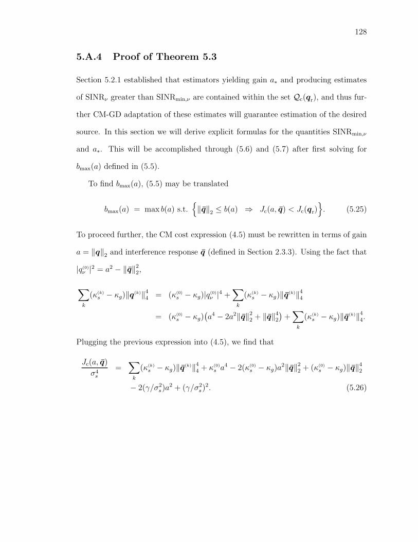
128

5.A.4 Proof of Theorem 5.3

Section 5.2.1 established that estimators yielding gain a∗ and producing estimates

of SINRν greater than SINRmin,ν are contained within the set Qc(qr), and thus fur-

ther CM-GD adaptation of these estimates will guarantee estimation of the desired

source. In this section we will derive explicit formulas for the quantities SINRmin,ν

and a∗. This will be accomplished through (5.6) and (5.7) after first solving for

bmax(a) defined in (5.5).

To find bmax(a), (5.5) may be translated

bmax(a) = max b(a) s.t.{

‖q‖2 ≤ b(a) ⇒ Jc(a, q) < Jc(qr)}

. (5.25)

To proceed further, the CM cost expression (4.5) must be rewritten in terms of gain

a = ‖q‖2 and interference response q (defined in Section 2.3.3). Using the fact that

|q(0)ν |2 = a2 − ‖q‖2

2,

∑

k

(κ(k)

s − κg)‖q(k)‖44 = (κ(0)

s − κg)|q(0)

ν |4 +∑

k

(κ(k)

s − κg)‖q(k)‖44

= (κ(0)

s − κg)(a4 − 2a2‖q‖2

2 + ‖q‖42

)+∑

k

(κ(k)

s − κg)‖q(k)‖44.

Plugging the previous expression into (4.5), we find that

Jc(a, q)

σ4s

=∑

k

(κ(k)

s − κg)‖q(k)‖44 + κ(0)

s a4 − 2(κ(0)

s − κg)a2‖q‖2

2 + (κ(0)

s − κg)‖q‖42

− 2(γ/σ2s)a

2 + (γ/σ2s)

2. (5.26)

129

From (5.11) and (5.26), the following statements are equivalent:

Jc(qr) > Jc(a, q)

0 >∑

k

(κ(k)

s − κg)‖q(k)‖44 + (κ(0)

s − κg)(

−2a2‖q‖22 + ‖q‖4

2

)

+ κ(0)

s a4 − 2

(γ

σ2s

)

a2 +

(γ

σ2s

)2(4

κ(0)s + κimin

s + 2κg

)

0 <1

κ(0)s − κg

∑

k

(κ(k)

s − κg)‖q(k)‖44 − 2a2‖q‖2

2 + ‖q‖42

+1

κ(0)s − κg

(

κ(0)

s a4 − 2

(γ

σ2s

)

a2 +

(γ

σ2s

)2(4

κ(0)s + κimin

s + 2κg

))

︸ ︷︷ ︸

C(a,qr)

.(5.27)

The reversal of inequality in (5.27) occurs because κ(0)s −κg < 0 (as implied by S4)).

Using the definition of κmaxs in (2.22), 0 ≤ ‖q(k)‖4

4

‖q(k)‖42

≤ 1 implies that

∑

k

(κ(k)

s − κg)‖q(k)‖44 ≤ (κmax

s − κg)‖q‖44 ≤

0, κmaxs ≤ κg

(κmaxs − κg)‖q‖4

2, κmaxs > κg.

(5.28)

Thus, with ρmax defined in (2.24), the following becomes a sufficient condition for

(5.27).

0 >

‖q‖42 − 2a2‖q‖2

2 + C(a, qr), κmaxs ≤ κg

(1 + ρmax)‖q‖42 − 2a2‖q‖2

2 + C(a, qr), κmaxs > κg.

(5.29)

Focusing first on the super-Gaussian case (κmaxs > κg), we see from (5.29) that

valid b2max(a) satisfying (5.25) can be determined by solving for the roots of

P1(x) = (1 + ρmax) x2 − 2a2x+ C(a, qr).

Specifically, we are interested in the smaller root when 1 + ρmax > 0 and the larger

root when 1 + ρmax < 0. In either of these two cases, the appropriate root has the

130

form

b2max(a) = a2

1 −

√

1 − (ρmax + 1)C(a,qr)a4

ρmax + 1

. (5.30)

When 1 + ρmax = 0 instead, P1(x) becomes linear and

b2max(a) =C(a, qr)

2a2. (5.31)

As a valid interference power, we require that b2max(a) ∈ [0, a2]. Straightforward

manipulations show that, for all valid super-Gaussian values of ρmax (i.e., ρmax < 0),

b2max(a) ∈ [0, a2] ⇔ 0 ≤ C(a, qr)

a4≤ 1 − ρmax. (5.32)

From (5.29) it can be seen that the same arguments may be applied to the

non-super-Gaussian case (κmaxs ≤ κg) by setting ρmax to zero. This yields

b2max(a) = a2

(

1 −√

1 − C(a, qr)

a4

)

(5.33)

with the requirement that 0 ≤ C(a, qr)/a4 ≤ 1.

The expressions for b2max(a) in (5.30), (5.31), and (5.33) can now be used to

calculate SINRmin,ν and a∗ given in (5.6) and (5.7). First we tackle the super-

Gaussian case (κmaxs > κg). Assuming for the moment that ρmax 6= −1, we plug

(5.30) into (5.6) to obtain

SINRmin,ν = mina

ρmax +√

1 − (ρmax + 1)C(a,qr)a4

1 −√

1 − (ρmax + 1)C(a,qr)a4

. (5.34)

Since the fraction on the right of (5.34) is non-negative and strictly decreasing in

C(a, qr)/a4 over the valid range C(a, qr)/a

4 ∈ [0, 1 − ρmax] identified by (5.32), find-

ing a that minimizes this expression [in accordance with (5.7)] can be accomplished

by finding a that maximizes C(a, qr)/a4. To find these maxima, we first write

C(a, qr)/a4 using (5.27):

C(a, qr)

a4= C0 + C1 · (a2)−1 + C2 · (a2)−2,

131

where C0, C1, and C2 are independent of a. Computing the partial derivative with

respect to the quantity a2 and setting it equal to zero, we find that

a2∗ = −2

C2

C1=

(γ

σ2s

)(4

κ(0)s + κimin

s + 2κg

)

. (5.35)

Plugging a2∗ into (5.27) and using the definition of ρimin in (5.9) gives the simple result

C(a∗, qr)/a4∗ = (3 − ρimin)/4. With this value of a∗, requirement (5.32) translates

into

κ(0)

s ≤ min

{κimin

s + 2κg

3, 4κmax

s − κimins − 2κg

}

. (5.36)

In the super-Gaussian case, we know that κ(0)s < 4κmax

s − κimins − 2κg, hence (5.36)

simplifies to

κ(0)

s ≤ κimins + 2κg

3.

Finally, plugging a∗ into (5.34) gives

SINRmin,ν =ρmax +

√

1 − (1 + ρmax)(3 − ρimin)/4

1 −√

1 − (1 + ρmax)(3 − ρimin)/4. (5.37)

Revisiting the super-Gaussian case with ρmax = −1, we plug (5.31) into (5.6)

and get

SINRmin,ν = mina

2

(C(a, qr)

a4

)−1

− 1.

Again, the quantity to be minimized is strictly decreasing in C(a, qr)/a4 over [0, 1−

ρmax]. As above, maximization of C(a, qr)/a4 yields the a∗ of (5.35) and the same

condition on κ(0)s . Applying these to the previous equation,

SINRmin,ν =5 + ρimin

3 − ρimin. (5.38)

For the non-super-Gaussian case (κmaxs ≤ κg), we plug (5.33) into (5.6) and

obtain

SINRmin,ν = mina

√

1 − C(a,qr)a4

1 −√

1 − C(a,qr)a4

. (5.39)

132

Since (5.39) equals (5.34) with ρmax = 0 (i.e., when κmaxs = κg), the non-super-

Gaussian will have the same a∗ as (5.35) and the same translation of (5.32) given by

(5.36). After substituting κmaxs = κg into (5.36), the non-super-Gaussian property

implies that condition (5.36) simplifies again to

κ(0)

s ≤ κimins + 2κg

3.

Plugging a∗ from (5.35) into (5.39), the non-super-Gaussian SINRmin,ν becomes

SINRmin,ν =

√1 + ρimin

2 −√1 + ρimin

. (5.40)

Finally, S1)-S3) imply that a = ‖q‖22 = σ2

y/σ2s , linking the critical gain a∗ in

(5.35) to the critical estimate variance σ2y

∣∣crit

in (5.10), yielding Theorem 5.3.

Chapter 6

Performance Bounds for

CM-Based Channel Identification1

6.1 Introduction

Consider Fig. 6.1 (or the left half of Fig. 2.3) where a desired source sequence {s(0)n }

combines linearly with K interferers through vector channels {h(0)(z), . . . ,h(K)(z)}.

We now consider the problem of estimating the impulse response coefficients of

channel {h(0)(z)}, rather than the symbol sequence {s(0)n }, knowing only the statistics

of the received signal {rn}. The literature refers to this problem as blind channel

identification [Tong PROC 98].

In Chapter 6 we analyze the performance of the blind channel identification

scheme of Fig. 6.2, whereby M-delayed versions of the CM-minimizing symbol

estimates {yn} ≈ {s(0)

n−ν} are cross-correlated with the vector received samples

{rn−Q, . . . , rn}, yielding the Q + 1 vector channel parameter estimates

{h(0)

ν+M−Q, . . . , h(0)

ν+M}. The δth parameter estimate h(0)

ν+M−δ can be expressed as

1The main results of this chapter also appear in the manuscript [Schniter TSP tbd].

133

134

h(0)(z)

h(1)(z)

...

h(K)(z)

desired{

s(0)n

noise &

interference

s(1)n

...

s(K)n

rn+

Figure 6.1: Linear system model with K sources of interference.

a biased version of the true parameter corrupted by an error term:

h(0)

ν+M−δ = E{rn−δy

∗n−M

}

= E

{∑

k,j

h(k)

j s(k)

n−δ−j

∑

`,i

q(`)∗i s(`)∗

n−M−i

}

= σ2s

∑

k,i

h(k)

i+M−δ q(k)∗i (6.1)

= σ2s q

(0)∗ν

︸ ︷︷ ︸

bias

(

h(0)

ν+M−δ +∑

(k,i)6=(0,ν)

h(k)

i+M−δ q(k)∗i /q(0)∗

ν

︸ ︷︷ ︸

error

)

.

rn

fc,ν(z)

h(0)

ν+M h(0)

ν+M−1 h(0)

ν+M−Q

yn yn−M

z−1z−1 z−1

z−M

E{·}E{·} E{·}

∗∗∗× × ×

· · ·

· · ·

Figure 6.2: Blind channel identification using CM estimates {yn} ≈ {s(0)

n−ν}.

We note that the identification scheme in Fig. 6.2 bears similarity to the Gooch-

135

Harp method of channel identification [Gooch ICC 88] in Fig. 6.3, whereby the CM

estimates {yn} are processed by a hard decision device D before cross-correlation.

Due to the nonlinear operation D, however, performance analysis of the Gooch-Harp

scheme is difficult unless perfect decision-making (i.e., dn = sn−ν) is assumed. In

addition, forming reliable decisions requires carrier phase synchronization (an issue

with passband data transmission [Proakis Book 95]) which is not required in the

identification scheme of Fig. 6.2.

rn

fc,ν(z)

h(0)

ν+M h(0)

ν+M−1 h(0)

ν+M−Q

Dyn dn dn−M

z−1z−1 z−1

z−M

E{·}E{·} E{·}

∗∗∗× × ×

· · ·

· · ·

Figure 6.3: Gooch-Harp method of blind channel identification.

Many other methods of blind channel identification have been proposed (see, e.g.,

the citations in [Tong PROC 98]), most of which estimate channel coefficients from

the observed data directly, i.e., without first forming blind symbol estimates. When

P > 1 and the channel satisfies certain conditions, it is possible to accomplish blind

identification using only the second-order statistics (SOS) of the observed process

(see, e.g., the references in [Liu SP 96]). Most SOS-based techniques, however,

are known to fail catastrophically when the channel order is overestimated (see,

e.g., the discussion in [Abed-Meraim TSP 97]). An exception is the approach in

[Abed-Meraim TSP 97] where, similar to Figs. 6.2 and 6.3, the channel coefficients

are estimated using cross-correlations with blind symbol estimates based on linear

prediction. The CM-based schemes in Figs. 6.2 and 6.3, however, do not rely on the

136

satisfaction of any channel-identifiability conditions.

In this chapter, we derive upper bounds for the average squared parameter error

(ASPE) of blind channel parameter estimates generated by the method of Fig. 6.2.

The bounds are a function of the channel coefficients, the source kurtoses, and the

symbol estimation delay. Next, we derive the expected ASPE that results when the

correlations in Fig. 6.2 are estimated from N -length data blocks. Finally, we discuss

the effect of stochastic-gradient symbol-estimator design (i.e., the use of CMA versus

exact gradient descent), as well as the effect of residual carrier offset in rn, on ASPE.

All results are derived in the multi-user vector-channel context of Section 2.2.

The organization of the chapter is as follows. Section 6.2 derives ASPE perfor-

mance bounds and Section 6.3 covers implementational issues such as finite data

effects, the use of CMA, and the presence of residual carrier offset. Section 6.4

presents the results of numerical simulations verifying our performance analyses,

and Section 6.5 concludes the chapter. Proofs and technical details have been rele-

gated to Appendix 6.A.

6.2 Blind Identification – Performance Bounds

We are interested in quantifying the sum-squared error of the Q+1 parameter esti-

mates {h(0)

ν+M−Q, . . . , h(0)

ν+M} relative to the true parameter subset

{h(0)

ν+M−Q, . . . ,h(0)

ν+M}. We tolerate arbitrary scaling of the total estimated chan-

nel response and define our average squared parameter error (ASPE) criterion as

137

follows.

Eh := minθ∈C

1

Q+1

Q∑

δ=0

∥∥∥θ h(0)

ν+M−δ − h(0)

ν+M−δ

∥∥∥

2

2(6.2)

= minθ∈C

1

Q+1

∥∥∥∥∥θ

(h

(0)ν+M

...h

(0)ν+M−Q

)

︸ ︷︷ ︸

h(0)ν+M

−(

h(0)ν+M

...h

(0)ν+M−Q

)

︸ ︷︷ ︸

h(0)ν+M

∥∥∥∥∥

2

2

. (6.3)

Note that by choosing M and Q large enough, an arbitrarily large subset of the

total channel response {h(0)n } may be estimated regardless of the symbol estimation

delay ν.

Theorem 6.1. For symbol estimation delay ν, the ASPE generated by the blind

channel identification scheme in Fig. 6.2 can be upper bounded as

Eh ≤‖HM ‖2 Ju,ν

∣∣max,Ju,ν(qm,ν)

c,ν

(Q+1)σ2s

(6.4)

≤E{‖rn‖2

2

}Ju,ν

∣∣max,Ju,ν(qm,ν)

c,ν

σ4s

(6.5)

when the Wiener symbol estimates satisfy the UMSE condition Ju,ν(qm,ν) ≤ Joσ2s

in Theorem 4.2.

When the channels and estimator are FIR, the quantity HM is a block Toeplitz

matrix closely related to H defined in (2.13). Specifically, HM has P (Q+1) rows

and Nq columns, where Nq denotes the length of q, with the following structure:

HM := (6.6)

h(0)

M · · · h(K)

M h(0)

M+1 · · · h(K)

M+1 · · · h(0)

M+Nq−1 · · · h(K)

M+Nq−1

h(0)

M−1 · · · h(K)

M−1 h(0)

M · · · h(K)

M · · · h(0)

M+Nq−2 · · · h(K)

M+Nq−2

......

......

......

h(0)

M−Q · · · h(K)

M−Q h(0)

M−Q+1 · · · h(K)

M−Q+1 · · · h(0)

M−Q+Nq−1 · · · h(K)

M−Q+Nq−1

.

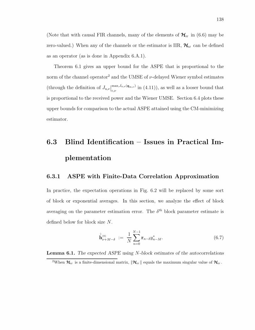
138

(Note that with causal FIR channels, many of the elements of HM in (6.6) may be

zero-valued.) When any of the channels or the estimator is IIR, HM can be defined

as an operator (as is done in Appendix 6.A.1).

Theorem 6.1 gives an upper bound for the ASPE that is proportional to the

norm of the channel operator2 and the UMSE of ν-delayed Wiener symbol estimates

(through the definition of Ju,ν

∣∣max,Ju,ν(qm,ν)

c,νin (4.11)), as well as a looser bound that

is proportional to the received power and the Wiener UMSE. Section 6.4 plots these

upper bounds for comparison to the actual ASPE attained using the CM-minimizing

estimator.

6.3 Blind Identification – Issues in Practical Im-

plementation

6.3.1 ASPE with Finite-Data Correlation Approximation

In practice, the expectation operations in Fig. 6.2 will be replaced by some sort

of block or exponential averages. In this section, we analyze the effect of block

averaging on the parameter estimation error. The δth block parameter estimate is

defined below for block size N .

ˆh(0)

ν+M−δ :=1

N

N−1∑

n=0

rn−δy∗n−M . (6.7)

Lemma 6.1. The expected ASPE using N -block estimates of the autocorrelations

2When HM is a finite-dimensional matrix, ‖HM ‖ equals the maximum singular value of HM .

139

can be written

E{Eˆ

h

}= Eh +

σ4s

N(Q+ 1)

|h(0)H

ν+Mh(0)

ν+M |2∥∥h

(0)

ν+M

∥∥

4

2

Q∑

δ=0

(∥∥∥∥

∑

k,i

√κ(k)s −1h(k)

i+M−δq(k)∗i

∥∥∥∥

2

2

+∑

p,k,j

h(k)Hj h(k)

j+p

∑

(`,i)6=(k,j+M−δ)

q(`)

i q(`)∗i+p

)

. (6.8)

Simulations suggest that, for CM-minimizing estimators fc,ν(z) and typical values

ofN , the second term in (6.8) dominates the first. This implies that the performance

of the proposed channel estimation scheme is in practice limited by the finite-data

correlations rather than by the performance of the blind symbol estimates. The

plots in Section 6.4 agree with this notion: improvement in symbol estimates gained

through quantization of {yn} gives the Gooch-Harp scheme [Gooch ICC 88] only

minor advantage in ASPE.

6.3.2 Stochastic Gradient Estimation of CM Equalizer

Practical implementations of the identification scheme in Fig. 6.2 will not have

knowledge of the exact CM-minimizing symbol estimator fc,ν(z). Typically, fc,ν(z)

will be replaced by an iteratively updated approximation to fc,ν(z) generated by

the constant modulus algorithm (CMA), an algorithm which attempts stochastic

gradient minimization of CM cost [Godard TCOM 80, Treichler TASSP 83]. For

finite-length f(z), CMA updates the equalizer parameters {f0, . . . , fNf−1} using the

following rule (where n denotes the time step).

fi(n+ 1) = fi(n) + µrn−iy∗n

(γ − |yn|2

), 0 ≤ i ≤ Nf − 1. (6.9)

Similar update rules can be derived for equalizer structures that employ feedback

(resulting in an IIR equalizer) [Endres SPAWC 99]. In (6.9), µ is a small positive

stepsize.

140

The operation of CMA can be considered as a two-stage process. Starting from

an initialization fi(z), the CMA-updated estimator f(z) first converges to a neigh-

borhood of the exact CM-minimizing estimator fc,ν(z) associated with some combi-

nation of source k and symbol estimation delay ν. The particular {source, delay},

as well as the time to convergence, depend on the initialization fi(z). Though

various initialization procedures have been proposed (see, e.g., the references in

[Johnson PROC 98]), none are known to work “perfectly” in all situations. In

Chapter 5 of this thesis, however, we have shown that if the signal to interference-

plus-noise (SINR) ratio of the estimates generated by fi(z) is above a prescribed

threshold, then small stepsize CMA will converge to a neighborhood of the CM-

minimum fc,ν(z) associated with the same {source, delay} as fi(z). Furthermore,

for i.i.d. sub-Gaussian sources in the presence of AWGN, we have shown that this

SINR threshold equals 3.8 dB.

Once the CMA-updated equalizer parameters have converged to a neighborhood

of the local CM minimum fc,ν(z), averaging theory predicts that the CMA-updated

equalizer trajectory converges almost surely and in mean to fc,ν(z) [Ljung Book 99].

In practical situations, however, the CMA-updated equalizer will “jitter” around

this local minimum, where the amount of jitter is proportional to the stepsize µ

and to the average size of the error term(γ − |yn|2

)in (6.9). It is possible to

derive expressions for the excess MSE due to CMA, i.e., the difference between the

expected MSE of CMA-generated symbol estimates and the MSE of CM-minimizing

estimates. For example, CMA’s excess MSE resulting from the use of source symbols

drawn from a non-constant-modulus alphabet is characterized in [Fijalkow TSP 98].

The simulations in Section 6.4, however, seem to indicate that for typical block

sizes N , the effects of finite-data correlation approximation overwhelm the effects

141

of CMA-induced excess symbol estimation error. For this reason, we do not further

investigate CMA-induced error.

Throughout our discussion of blind channel estimation we have been assuming

that the CMA-derived symbol estimates are reasonably accurate, which would seem

to require use of a data record long enough to support the convergence time of

CMA. Even with very short data records, however, it may be possible to adapt

CMA using a repeatedly concatenated version of the same data record (similar to

“looped” LMS [Qureshi PROC 85]). Since source independence assumptions S1)–

S2) become less valid as record length decreases, however, it is difficult to make

solid claims about the convergence of such data-reusing CMA schemes. Though of

practical importance, CMA data-reuse lies outside the scope of this thesis.

6.3.3 Effect of Residual Carrier Offset

In passband communication systems, it is typically the case that the receiver’s

down-conversion frequency is not exactly equal to the transmitter’s up-conversion

frequency, so that the quasi-baseband received signal {rn} contains residual carrier

frequency offset [Proakis Book 95]. This phenomenon changes the received signal

model (2.6), shown in Fig. 6.1, to (6.10), shown in Fig. 6.4, for an offset frequency

of ω radians per symbol-period.

rn =

K∑

k=0

∞∑

i=0

h(k)

i s(k)

n−iejωn. (6.10)

Throughout this subsection, we assume that the channel, equalizer, and source

quantities are all complex-valued and use j to denote√−1.

142

h(0)(z)

h(1)(z)

...

h(K)(z)

desired{

s(0)n

noise &

interference

s(1)n

...

s(K)n

rn+ ×

∼ ejωn

Figure 6.4: Linear system model with residual carrier offset

From (6.10), the symbol estimates become

yn =

∞∑

m=−∞fHm rn−m

=∑

m,i,k

fHm h(k)

i s(k)

n−m−iejω(n−m)

= ejωn∑

k,i

(∑

m

fHm e

−jωmh(k)

i−m

︸ ︷︷ ︸

q(k)

i

)

s(k)

n−i, (6.11)

which implies that the identification scheme in Fig. 6.2 returns the following channel

parameter estimates.

h(0)

ν+M−δ = E{rn−δy

∗n−M

}

= E

{∑

k,p

h(k)

p s(k)

n−δ−pejω(n−δ) · e−jωn

∑

`,i

q(`)∗i s(`)∗

n−M−i

}

= σ2se

−jωδ∑

k,i

h(k)

i+M−δ q(k)∗i . (6.12)

From (2.35) it is apparent that the CM criterion is insensitive to symbol estimate

phase. Equation (6.11) then implies that qc,ν in the presence of carrier offset should

equal qc,ν in the absence of offset (via fc,ν(z) in the presence of offset equaling fc,ν(z)

in the absence of offset after rotation of themth impulse response coefficient by ejωm).

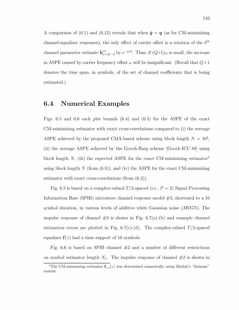
143

A comparison of (6.1) and (6.12) reveals that when q = q (as for CM-minimizing

channel-equalizer responses), the only effect of carrier offset is a rotation of the δth

channel parameter estimate h(0)

ν+M−δ by e−jωδ. Thus, if (Q+1)ω is small, the increase

in ASPE caused by carrier frequency offset ω will be insignificant. (Recall that Q+1

denotes the time span, in symbols, of the set of channel coefficients that is being

estimated.)

6.4 Numerical Examples

Figs. 6.5 and 6.6 each plot bounds (6.4) and (6.5) for the ASPE of the exact

CM-minimizing estimator with exact cross-correlations compared to (i) the average

ASPE achieved by the proposed CMA-based scheme using block length N = 104,

(ii) the average ASPE achieved by the Gooch-Harp scheme [Gooch ICC 88] using

block length N , (iii) the expected ASPE for the exact CM-minimizing estimator3

using block length N (from (6.8)), and (iv) the ASPE for the exact CM-minimizing

estimator with exact cross-correlations (from (6.2)).

Fig. 6.5 is based on a complex-valued T/2-spaced (i.e., P = 2) Signal Processing

Information Base (SPIB) microwave channel response model #3, shortened to a 16

symbol duration, in various levels of additive white Gaussian noise (AWGN). The

impulse response of channel #3 is shown in Fig. 6.7(a)-(b) and example channel

estimation errors are plotted in Fig. 6.7(c)-(d). The complex-valued T/2-spaced

equalizer f(z) had a time support of 10 symbols.

Fig. 6.6 is based on SPIB channel #2 and a number of different restrictions

on symbol estimator length Nf . The impulse response of channel #2 is shown in

3The CM-minimizing estimator fc,ν(z) was determined numerically using Matlab’s “fminunc”routine.

144

Fig. 6.8(a)-(b) and example channel estimation errors are plotted in Fig. 6.8(c)-(d).

The SNR of AWGN was 40 dB.

The following were common to all experiments: the desired source was i.i.d. and

drawn from a 64-QAM alphabet; ν was the MSE-minimizing symbol delay for the

particular combination of channel, noise, and equalizer constraints; Q and M were

adjusted so that all 32 T/2-spaced coefficients of the SPIB channel were estimated;

and CMA was initialized at fc,ν(z) and adapted with stepsize µ = 10−3.

The fact that the upper-bound-(6.4) trace crosses the N -block traces in Figs. 6.5

and 6.6 should not cause alarm: (6.4) bounds the ASPE assuming exact cross-

correlations, while the CMA, Gooch-Harp, and CM-N traces assume length-N block

approximations of the cross-correlations.

6.5 Conclusions

We have analyzed the performance of a blind channel identification scheme based

on the cross-correlation of CM-minimizing blind symbol estimates with the received

signal. Leveraging recent results on the unbiased MSE of CM-minimizing symbol

estimates, upper bounds on the average squared channel parameter estimation error

(ASPE) were derived. Various implementational aspects were also considered, such

as ASPE increase due to finite-data correlator approximations, stochastic gradient

estimates of the CM-minimizing equalizer, and residual carrier frequency offset.

Finally, experiments using SPIB microwave channel models were presented to verify

the results of our analyses.

145

10 15 20 25 30 35 40 45 50−80

−70

−60

−50

−40

−30

−20

−10

0

SNR−AWGN [dB]

MS

PE

[dB

]

bound (6.5) bound (6.4) CMA:N CM:N CM:N→ infGooch:N

Figure 6.5: Mean-squared parameter error for 32-tap T/2-spaced SPIB microwave

channel #3 versus SNR of AWGN.

146

2 3 4 5 6 7 8 9 10−50

−45

−40

−35

−30

−25

−20

Nf

MS

PE

[dB

]

bound (6.5) bound (6.4) CMA:N CM:N CM:N→ infGooch:N

Figure 6.6: Mean-squared parameter error for 32-tap T/2-spaced SPIB microwave

channel #3 versus symbol estimator length Nf .

147

0 5 10 15 20 25 30 35−0.2

0

0.2

0.4

0.6

0.8

real

cha

nnel

(a)

0 5 10 15 20 25 30 35−0.1

−0.05

0

0.05

0.1

imag

cha

nnel

(b)

0 5 10 15 20 25 30 35−2

−1

0

1

2x 10

−3

real

err

or

(c)

CMA:N Gooch:N CM:N→ inf

0 5 10 15 20 25 30 35−1.5

−1

−0.5

0

0.5

1x 10

−3

imag

err

or

(d)

CMA:N Gooch:N CM:N→ inf

Figure 6.7: (a) Real and (b) imaginary components of 32-tap T/2-spaced SPIB

microwave channel #3 impulse response. (c) Real and (d) imaginary components

of estimation errors for SNR = 50 dB and Nf = 10.

148

0 5 10 15 20 25 30 35−0.2

0

0.2

0.4

0.6

0.8

real

cha

nnel

(a)

0 5 10 15 20 25 30 35−0.1

−0.05

0

0.05

0.1

0.15

imag

cha

nnel

(b)

0 5 10 15 20 25 30 35−15

−10

−5

0

5x 10

−3

real

err

or

CMA:N Gooch:N CM:N→ inf

0 5 10 15 20 25 30 35−4

−3

−2

−1

0

1

2x 10

−3

imag

err

or

(d)

CMA:N Gooch:N CM:N→ inf

Figure 6.8: (a) Real and (b) imaginary components of 32-tap T/2-spaced SPIB

microwave channel #2 impulse response. (c) Real and (d) imaginary components

of estimation errors for SNR = 40 dB and Nf = 10.

149

Appendix

6.A Derivation Details for Channel Identification

Bounds

This appendix contains proofs of the theorem and lemma found in Section 6.2 and

Section 6.3, respectively.

6.A.1 Proof of Theorem 6.1

To ensure that our bound applies to both finite and infinite-dimensional channels and

estimators, we formalize the definition of the operator H (whose finite-dimensional

definition appeared in (6.6)).

HM : `1(CP ) → CP (Q+1) s.t. HM q =

∑

k,i h(k)

i+Mq(k)

i

∑

k,i h(k)

i+M−1q(k)

i

...

∑

k,i h(k)

i+M−Qq(k)

i

. (6.13)

Recall that q and `1(CP ) were defined in Section 2.2. When h(k)(z) are FIR, HM

reduces to a block Toeplitz matrix. The operator HM will also prove useful:

HM : `1(CP ) → CP (Q+1) s.t. HM q =

∑

(k,i)6=(0,ν) h(k)

i+Mq(k)

i

∑

(k,i)6=(0,ν) h(k)

i+M−1q(k)

i

...

∑

(k,i)6=(0,ν) h(k)

i+M−Qq(k)

i

. (6.14)

HM is a version of HM with the components for the 0th source at delay ν removed,

and q is a version of q with the q(0)ν element extracted.

150

Using (6.1) and the definitions of h(0)

ν+M and h(0)

ν+M in (6.3), the operators HM

and HM allow us to write

h(0)

ν+M = HM q∗σ2s

= HM q∗σ2s + h

(0)

ν+Mq(0)∗ν σ2

s . (6.15)

Choosing θ = (q(0)∗ν σ2

s)−1 in (6.3),

Eh ≤ 1

Q+1

∥∥∥∥∥

h(0)

ν+M

q(0)∗ν σ2

s

− h(0)

ν+M

∥∥∥∥∥

2

2

=1

Q+1

∥∥HM q∗∥∥2

2

|q(0)ν |2 . (6.16)

Definition of the induced norm

‖HM ‖ := supq6=0

‖HM q∗‖2

‖q‖2

(6.17)

(which, for finite-dimensional HM , equals the largest singular value) allows further

bounding of (6.16):

Eh ≤ 1

Q+1

‖HM ‖2‖q‖22

|q(0)ν |2 . (6.18)

Recalling the definition of UMSE in (2.31), equation (6.18) becomes

Eh ≤ Ju,ν(qc,ν)‖HM ‖2

(Q+1)σ2s

. (6.19)

When {h(k)(z)}, Qa, and ν are such that Ju,ν(qm,ν) ≤ Joσ2s for Jo in (4.10), Theo-

rem 4.2 allows upper bounding of Ju,ν(qc,ν) and (6.19) becomes

Eh ≤ Ju,ν

∣∣max,Ju,ν(qm,ν)

c,ν

‖HM ‖2

(Q+1)σ2s

. (6.20)

Since

‖HM ‖2 = sup‖q‖2=1

qtH

HM

HM q∗

≥ sup‖q‖2=1, q

(0)ν =0

qtH

HM

HM q∗

= sup‖q‖2=1

qtH

HM

HM q∗

= ‖HM ‖2,

151

(6.20) yields

Eh ≤ Ju,ν

∣∣max,Ju,ν(qm,ν)

c,ν

‖HM ‖2

(Q+1)σ2s

. (6.21)

Simplification of (6.21) is possible using the fact that

‖HM q∗‖22 =

Q∑

δ=0

∥∥∥∥

∑

k,i

h(k)

i+M−δ q(k)∗i

∥∥∥∥

2

2

≤Q∑

δ=0

(∑

k,i

‖h(k)

i+M−δ q(k)∗i ‖2

2

)

=

Q∑

δ=0

∑

k,i

‖h(k)

i+M−δ‖2

2|q(k)

i |2

≤ (Q+1)∑

k,i

‖h(k)

i ‖2

2 ‖q‖22

which implies

‖HM ‖2 ≤ (Q+1)∑

k,i

‖h(k)

i ‖2

2. (6.22)

Rewriting (6.22) using

∑

k,i

‖h(k)

i ‖2

2 =1

σ2s

E

{∥∥∥

∑

k,i

h(k)

i s(k)

n−i

∥∥∥

2

2

}

=1

σ2s

E{‖rn‖2

2

}

gives

‖HM ‖22 ≤ Q+ 1

σ4s

E{‖rn‖2

2

}, (6.23)

which, combined with (6.21), leads to (6.5).

6.A.2 Proof of Lemma 6.1

The mean of the block parameter estimate is

E{

ˆh(0)

ν+M−δ

}

= E{rn−δy∗n−M} = h(0)

ν+M−δ, (6.24)

152

implying a variance of the form

var(

ˆh(0)

ν+M−δ

)

= E

{∥∥∥ˆh(0)

ν+M−δ − h(0)

ν+M−δ

∥∥∥

2

2

}

.

Rewriting (6.7) using expressions from Section 2.2

ˆh(0)

ν+M−δ =1

N

N−1∑

n=0

∑

k,j

h(k)

j s(k)

n−δ−j

∑

`,i

q(`)∗i s(`)∗

n−M−i

=∑

k,j,`,i

h(k)

j q(`)∗i

1

N

N−1∑

n=0

s(k)

n−δ−js(`)∗n−M−i

=∑

k,i

h(k)

i+M−δq(k)∗i

1

N

N−1∑

n=0

|s(k)

n−M−i|2

+∑

k,j

∑

(`,i)6=(k,j+M−δ)

h(k)

j q(`)∗i

1

N

N−1∑

n=0

s(k)

n−δ−js(`)∗n−M−i (6.25)

and recalling (6.1), the variance can be rewritten as

var(

ˆh(0)

ν+M−δ

)

= E

{∥∥∥∥

∑

k,i

h(k)

i+M−δq(k)∗i

(1

N

N−1∑

n=0

|s(k)

n−M−i|2 − σ2s

)

+∑

k,j

∑

(`,i)6=(k,j+M−δ)

h(k)

j q(`)∗i

1

N

N−1∑

n=0

s(k)

n−δ−js(`)∗n−M−i

∥∥∥∥

2

2

. (6.26)

It can be shown that

E

{(1

N

N−1∑

n=0

|s(k)

n |2 − σ2s

)2}

=(κ(k)

s − 1)

Nσ4

s , (6.27)

E

{(1

N

N−1∑

n=0

|s(k)

n−a|2 − σ2s

)1

N

N−1∑

m=0

s(k)∗m−js

(`)

m−i

}

=

nonzero (k, j) = (`, i)

0 else,

(6.28)

153

and

E

{(1

N

N−1∑

n=0

s(a)

n−bs(c)∗n−d

)(1

N

N−1∑

m=0

s(k)∗m−js

(`)

m−i

)}

=

nonzero (a, b) = (c, d) and (k, j) = (`, i)

σ4s

N∃ p s.t. (a, b) = (k, j+p) 6= (c, d) = (`, i+p)

0 else.

(6.29)

Plugging (6.27)-(6.29) into (6.26), we see that the terms labeled “nonzero” in (6.27)-

(6.29) do not enter into the variance expression. Collected, the remaining terms yield

(6.30).

var(

ˆh(0)

ν+M−δ

)

=σ4

s

N

(∥∥∥∥

∑

k,i

√

κ(k)s −1h(k)

i+M−δq(k)∗i

∥∥∥∥

2

2

+∑

p

∑

k,j

h(k)Hj h(k)

j+p

∑

(`,i)6=(k,j+M−δ)

q(`)

i q(`)∗i+p

. (6.30)

In terms of the N -block variance (6.30), the expected block-MSPE can be written

E{Eˆ

h

}= E

{

1

Q+ 1

Q∑

δ=0

∥∥∥θh

ˆh(0)

ν+M−δ − h(0)

ν+M−δ

∥∥∥

2

2

}

= E

{

1

Q+ 1

Q∑

δ=0

(∥∥∥θh

ˆh(0)

ν+M−δ − θh E{

ˆh(0)

ν+M−δ

}∥∥∥

2

2

+∥∥∥θh E

{ˆh(0)

ν+M−δ

}

− h(0)

ν+M−δ

∥∥∥

2

2

)}

=1

Q+ 1

Q∑

δ=0

(

|θh|2 E

{∥∥∥ˆh(0)

ν+M−δ − h(0)

ν+M−δ

∥∥∥

2

2

}

+∥∥∥θhh

(0)

ν+M−δ − h(0)

ν+M−δ

∥∥∥

2

2

)

= Eh +|θh|2Q+ 1

Q∑

δ=0

var(

ˆh(0)

ν+M−δ

)

where θh is the value of θ minimizing Eh in (6.2). It is straightforward to show that

θh =h

(0)H

ν+Mh(0)

ν+M∥∥h

(0)

ν+M

∥∥

2

2

.

Chapter 7

Dithered Signed-Error CMA1

7.1 Introduction

The constant modulus algorithm (CMA), conceived independently in

[Godard TCOM 80] and [Treichler TASSP 83], is a stochastic gradient algorithm

minimizing the CM criterion: Jc = E{(|yn|2 − γ)2

}. The positive constant γ is re-

ferred to as the dispersion constant and can be chosen in accordance with the source

statistics when they are known. As an iterative update algorithm of FIR estimator

f , CMA takes the form

f (n+ 1) = f (n) + µr∗(n) yn

(γ − |yn|2

)

︸ ︷︷ ︸

:= ψ(yn)

, (7.1)

where µ is a (small) positive step-size. The function ψ(·) identified in (7.1) is referred

to as the CMA error function and will appear many times throughout this chapter.

Low-cost consumer applications (e.g., HDTV) motivate blind equalization tech-

1Based on “Dithered Signed-Error CMA: Robust, Computationally Efficient Blind Adaptive

Equalization” by P. Schniter and C.R. Johnson, Jr., which appeared in IEEE Transactions on

Signal Processing; vol. 47, no. 6, pp. 1592-1603; June 1999. c©1999 IEEE. (With permission.)

154

155

niques requiring minimum implementation cost. Although noted for its LMS-like

complexity, CMA may be further simplified by transforming the bulk of its update

multiplications into sign operations [Treichler TASSP 83]. A recent study suggests,

however, that straightforward implementations of signed-error CMA (SE-CMA) do

not inherit the desirable robustness properties of CMA [Brown ALL 97]. In this

chapter we present a simple modification of SE-CMA, based on the judicious in-

corporation of controlled noise (sometimes referred to as “dither”), that results in

an algorithm with robustness properties closely resembling the standard (unsigned)

CMA. In fact, we show that the mean behavior of dithered signed-error CMA (DSE-

CMA) is identical to CMA under realistically achievable conditions. The anticipated

drawback to this dithering is a degradation in steady-state mean-square error (MSE)

performance. Hence, we derive an expression for the excess MSE (EMSE) of DSE-

CMA and discuss implications on step-size and equalizer-length selection. We note

in advance that the EMSE expression for DSE-CMA bears close resemblance to an

analogous expression derived for CMA in [Fijalkow TSP 98].

The chapter is partitioned as follows: Section 7.2 reviews CMA, discusses compu-

tationally-efficient versions of CMA, and introduces the new algorithm. The tran-

sient and steady-state properties of DSE-CMA are studied in Section 7.3 and result

in the design guidelines of Section 7.4. Simulation results based on SPIB microwave

channel models are presented in Section 7.5. Section 7.5 also includes a comparison

study with a different robust and computationally-constrained implementation of

CMA.

For simplicity, this chapter assumes the case of real-valued quantities2 and FIR

estimators. Recall from Section 4.1 that under these assumptions, the satisfaction of

2Extension to the complex-valued case is straightforward—see Section 7.6.

156

S1)–S4) and the presence of full column rank (FCR) H (in the model of Section 2.2)

are sufficient to guarantee that CM minimization yields perfect blind estimates, i.e.,

perfect estimates modulo unavoidable gain and delay ambiguities. In addition, we

assume that the source statistic ratio E{|s(0)n |4}/E{|s(0)

n |2} is known since this allows

removal of the gain ambiguity via the choice γ = γ? for

γ? =E{|s(0)

n |4}E{|s(0)

n |2} . (7.2)

7.2 Computationally Efficient CMA

Straightforward implementations of LMS-like adaptive algorithms (such as CMA)

require a multiplication between the error function and every regressor element (see

update equation (7.1)). Many practical applications benefit from eliminating these

Nf regressor multiplies. Signed-error (SE) algorithms present one method for doing

so, whereby only the sign of the error function is retained [Macchi Book 95]. When

a SE algorithm is combined with a power-of-two step-size, it is possible to construct

a multiply-free fixed-point implementation of the equalizer update algorithm. The

subsections below discuss two versions of SE-CMA. (For the remainder of the chap-

ter, we restrict our focus to the case where all quantities are real-valued. Extensions

to the complex-valued case are briefly discussed in Section 7.6.)

7.2.1 Signed-Error CMA

The real-valued SE-CMA algorithm [Treichler TASSP 83] is specified as

f(n + 1) = f (n) + µr(n) sgn(yn(γ − y2

n))

︸ ︷︷ ︸

:= ξ(yn)

, (7.3)

157

where sgn(·) denotes the standard signum function. Equation (7.3) defines the SE-

CMA error function ξ(·), depicted in Fig. 7.1.

−2 −1.5 −1 −0.5 0 0.5 1 1.5 2−2

−1.5

−1

−0.5

0

0.5

1

1.5

2

CMA SE−CMA DSE−CMA, α=1.5

Figure 7.1: CMA, SE-CMA, and DSE-CMA error functions.

A recent investigation into SE-CMA has shown that, while satisfaction of FCR

H and the selection γ = γ? ensure mean convergence to perfectly scaled blind

estimates, the presence of non-FCR H can severely hinder SE-CMA convergence

behavior [Brown ALL 97]. Specifically, there may exist vast yet highly suboptimal

regions in equalizer space in which the expected update in (7.3) is zero. Fig. 7.2

presents an example3 of such behavior, in which the trajectory labelled “B” appears

not to converge. (See Fig. 7.6 for examples of CMA trajectories under identical

3In Fig. 7.2, BPSK was transmitted over the following noiseless FIR vector channel: {hn} ={(

0.10.3

),(

1−0.1

),(

0.50.2

)}.

158

conditions.) Thus, while computationally efficient, SE-CMA does not inherit the

−1.5 −1 −0.5 0 0.5 1 1.5 2 2.5−0.2

0

0.2

0.4

0.6

0.8

1

f0

f1

CM Error Surface

A

B

Figure 7.2: SE-CMA trajectories superimposed on Jc cost contours. Dotted lines

delineate SE-CMA constant-gradient facets.

desirable robustness properties of CMA. This fact motivates the search for com-

putationally efficient blind algorithms which do inherit these robustness properties.

The following section describes one such algorithm.

7.2.2 Dithered Signed-Error CMA

“Gimme noise, noise, noise, noise . . . ”

—The Replacements, Stink, 1982.

Viewing the SE-CMA error function as a one bit quantizer, one might wonder

159

whether a suitable dithering technique [Gray TIT 93] would help to remove the

unwanted behavioral artifacts caused by the sign operator4. Dithering refers to

the addition of a random signal before quantization in an attempt to preserve the

information lost in the quantization process. From an additive noise perspective,

dithering is an attempt to make the so-called quantization noise (see Fig. 7.3) white,

zero-mean, and independent of the signal being quantized. One might expect that

such quantization noise could be “averaged out” by a small step-size adaptive algo-

rithm, yielding mean behavior identical to that of its unsigned counterpart. These

ideas are made precise in Section 7.3.2.

The real-valued dithered signed-error constant modulus algorithm (DSE-CMA)

is defined by the update

f(n + 1) = f (n) + µ r(n)α sgn(yn(γ − y2

n) + αdn

)

︸ ︷︷ ︸

:= ϕα(yn, dn)

, (7.4)

where {dn} is an i.i.d. “dithering” process uniformly distributed on (-1,1], both γ

and α are positive constants, and ϕα(yn, dn) is the DSE-CMA error function. The

practical selection of the dispersion constant γ and the “dither amplitude” α are

discussed in Section 7.4. It should become clear in the next section why α appears

twice in (7.4).

In the sequel we shall see that the mean behavior of DSE-CMA closely matches

that of standard (unsigned) CMA.

4The authors acknowledge a previous application of controlled noise to SE-LMS in the contextof echo cancellation [Holte TCOM 81], [Bonnet ICASSP 84]. However, both the analyses and goalswere substantially different than those in this chapter.

160

7.3 The Fundamental Properties of DSE-CMA

Sections 7.3.2–7.3.4 utilize an additive noise model of the dithered sign operation

to characterize the transient and steady-state behaviors of DSE-CMA. Before pro-

ceeding, we present the details of this quantization noise model.

7.3.1 Quantization Noise Model of DSE-CMA

At first glance, the nonlinear sign operator in (7.4) appears to complicate the behav-

ioral analysis of DSE-CMA. Fortunately, the theory of dithered quantizers allows

us to subsume the sign operator by adopting a quantization-noise model of the

DSE-CMA error function (see Fig. 7.3). Appendix 7.A collects the key results from

classical quantization theory that allow us to formulate this model.

+ +xnxn

dn εn

Q

Figure 7.3: Quantization noise model (right) of the dithered quantizer (left).

DSE-CMA can be connected to the quantization literature with the observa-

tion that the operator α sgn(·) is identical to the two-level uniform quantizer Q(·),

specified by

Q(x) =

∆/2 x ≥ 0,

−∆/2 x < 0,

(7.5)

for quantizer spacing ∆ = 2α. Furthermore, the specification that {dn} be uniformly

distributed on (−1, 1] ensures that {αdn} satisfies the requirements for a valid dither

161

process outlined in Appendix 7.A, so long as α is selected large enough to satisfy

α ≥∣∣ψ(yn)

∣∣ (7.6)

for relevant values of the equalizer output yn. Recall that ψ(·) denotes the CMA

error function, defined in (7.1).

Employing the model of Fig. 7.3, we write the DSE-CMA error function in terms

of the quantization noise εn,

ϕα(yn, dn) = ψ(yn) + εn, (7.7)

which leads to the following DSE-CMA update expression:

f (n+ 1) = f(n) + µr(n)(ψ(yn) + εn

). (7.8)

When α and yn satisfy (7.6), the properties of εn follow from equations (7.29), (7.30),

and (7.32) in Appendix 7.A. Specifically, we have that εn is an uncorrelated random

process whose first moment obeys

E{εn∣∣ψ(yn)

}= E{εn} = 0, (7.9)

and whose conditional second moment is given by

E{ε2n∣∣ψ(yn)

}= α2 − ψ2(yn). (7.10)

In (7.9) and (7.10), the expectation is taken over the dither process, thus leaving a

dependence on yn.

7.3.2 DSE-CMA Transient Behavior

The average transient behavior of DSE-CMA is completely determined by the ex-

pected DSE-CMA error function, ϕα(yn) := E{ϕα(yn, dn)

∣∣yn

}. Equations (7.6)–

(7.9) indicate that ϕα(·) is a “hard-limited” version of the CMA error function,

162

ψ(·), i.e.,

ϕα(y) =

α y : ψ(y) > α,

ψ(y) y : |ψ(y)| ≤ α,

−α y : ψ(y) < −α.

(7.11)

Fig. 7.1 plots the various error functions ϕα(·), ψ(·), and ξ(·) for comparison. In

the theorems below, the implications of (7.11) are formalized in terms of DSE-CMA

behavior over specific ranges of α.

Lemma 7.1. Define

αC := 2(γ/3)3/2. (7.12)

The choice of dither amplitude α > αC ensures that ϕα(y) = ψ(y) for all equalizer

outputs y satisfying the output amplitude constraint: |y| ≤ ψ−1(α).

Proof. By evaluating ψ at the locations where ψ′ = 0, it can be seen that the

“humps” of the cubic CMA error function (see Fig. 7.1) occur at heights ±2(γ/3)3/2.

Thus, ψ−1(α) is unique and well-defined for α > 2(γ/3)3/2 = αC. Since (7.11)

implies that such values of α prevent these humps from being clipped in forming

the expected DSE-CMA error function, ϕα and ψ are identical over the interval

[−ψ−1(α), ψ−1(α)] when α > 2(γ/3)3/2.

For values α > αC, ψ−1(α) is determined by the unique real-valued root of the

cubic polynomial −y3 + γy + α and can be expressed as

ψ−1(α) = (7.13)

1

6

(

12√

81α2 − 12γ3 − 108α)1

3+ 2γ

(

12√

81α2 − 12γ3 − 108α)− 1

3.

From Equation (7.13), it can be shown that limα→α+Cψ−1(α) = 2

√

γ/3.

163

Writing the system output as y = rtf for a (fixed) received vector r and arbitrary

equalizer f allows the following equalizer-space interpretation of Lemma 7.1:

Theorem 7.1. Denote the set of possible received vectors by R, and define Fα to be

the convex hull formed by the set of hyperplanes Bα := {f : |rtf | = ψ−1(α) for r ∈

R}. Then choice of dither amplitude α > αC ensures that the expected DSE-CMA

update is identical to the CMA update for equalizers within Fα.

Proof. Choose any two equalizers f1 and f2 that satisfy the output constraint

|rtf | ≤ ψ−1(α) for all r ∈ R. (Recall ψ−1(α) is well defined for α > αC.) The

triangle inequality implies that any convex combination of f 1 and f2 also satisfies

this output constraint. Lemma 7.1 ensures that, for y = rtf that satisfy the output

amplitude constraint, ϕα(y) = ψ(y). Hence, the two updates are identical within

Fα.

For an M-ary source, the set S of possible source vectors s is of size MNq . Then,

in the absence of channel noise, we expect at most MNq equalizer input vectors

r = Hts. Hence, in this noiseless case, Fα is the convex hull formed by the finite

set of MNq hyperplanes Bα = {f : |stHf | = ψ−1(α) for s ∈ S}. In other words, Fα

is a polytope formed by the boundary set Bα. An illustrative example of Fα and Bα

is provided by Fig. 7.5.

Next, we concern ourselves with neighborhoods of the zero-forcing (ZF) equaliz-

ers {f δ : 0 ≤ δ < Nq} which have the property f tδH = et

δ. The ZF equalizers exist

when H is FCR.

Theorem 7.2. Define

αZF := maxs∈S

|ψ(s)|. (7.14)

164

Under FCR H, choice of dither amplitude α > αZF ensures the existence of a neigh-

borhood around every ZF solution f δ within which the expected DSE-CMA update

is identical to the CMA update.

Proof. When f = f δ, we know yn = sn−δ for all sn. In this case, (7.11) and the

definition of αZF imply that ψ(yn) = ϕα(yn) for α ≥ αZF. In other words, α ≥ αZF

guarantees that the expected DSE-CMA update is identical to the CMA update at

the zero-forcing solutions.

Now, consider an open ball B of radius ρ centered at f δ. Equalizers within B can

be parameterized as f = f δ + f for ‖f‖ < ρ. Then there exists a finite constant K

for which |yn−sn−δ| ≤ maxs∈S |stHf | < Kρ. From the continuity of the polynomial

function ψ(·), we claim the following: for any ε := α − αZF > 0 and any r ∈ R,

there exists a ρ > 0 such that ‖f‖ < ρ implies |ψ(rtf) − ψ(rtfδ)| < ε. Applying

(7.11), we conclude that ψ = ϕα for any equalizer within the ball B.

Note that the constant αZF may be less than αC, in which case there would exist

isolated “CMA-like” neighborhoods around the ZF solutions—i.e., neighborhoods

not contained in any “CMA-like” convex hull.

Theorem 7.2 is of limited practical use since it requires FCR H. Fortunately,

the concept is easily extended to the set of “open-eye” equalizers, FOE. Denoting

the minimum distance between any pair of adjacent symbols in S by ∆s, we define

the set FOE as5

FOE :={f : min

δmaxr∈R

rt(f − f δ) < ∆s/2}.

5We acknowledge that the definition of FOE is overly strict in that it bounds the outermostdecision region from both sides. In addition, the definition of FOE only makes sense in the contextof bounded inputs r. Although the AWGN channel model does not ensure bounded r, all practicalimplementations do.

165

The corresponding set of open-eye equalizer outputs is defined by

YOE :={y : min

s∈S|y − s| < ∆s/2

}.

For M-PAM, YOE becomes the open interval (−smax−smin, smax+smin) minus the set

of points halfway between adjacent elements of S. Here, smin and smax are used to

denote the minimum and maximum positive-valued elements of S, respectively.

Theorem 7.3. Define

αOE := maxy∈YOE

|ψ(y)|. (7.15)

Choice of dither amplitude α > αOE ensures the existence of a neighborhood around

every open-eye equalizer, f ∈ FOE, within which the expected DSE-CMA update is

identical to the CMA update.

Proof. The proof is identical to that of Theorem 7.2 after replacing s ∈ S by y ∈

YOE.

In summary, αC is the lower limit of α for which the convex set Fα exists, while

αZF and αOE are the lower limits of α for which “CMA-like” local neighborhoods

around the zero-forcing and open-eye equalizers exist, respectively. Table 7.1 quan-

tifies the values of {αC, αZF, αOE} for M-PAM alphabets, and Fig. 7.4 illustrates their

relationship to the CMA error function. Note that the difference between αZF and

αOE narrows as the alphabet size increases. This can be attributed to the fact that

the open-eye neighborhoods shrink as the constellation becomes more dense.

7.3.3 DSE-CMA Cost Surface

Studies of the multi-modal Jc cost surface give substantial insight into the transient

behavior of CMA (see, e.g., [Johnson PROC 98]). Thus, we expect that an exam-

ination of Jdse, the cost stochastically minimized by DSE-CMA, should also prove

166

−1 0 1

−3

−2

−1

0

1

2

3

4−PAM

ψ(yn)

ψ(sn)

αZF

αC

αOE

−1 0 1

−2.5

−2

−1.5

−1

−0.5

0

0.5

1

1.5

2

2.5

16−PAM

ψ(yn)

ψ(sn)

αZF

αC

αOE

Figure 7.4: CMA error function and critical values of α for 4-PAM and 16-PAM

sources.

Table 7.1: Critical values of α for M-PAM.

M 2 4 8 16 32

αC 0.38 0.81 0.90 0.92 0.93

αZF 0 0.64 0.87 1.39 1.71

αOE 6 2.79 2.24 2.12 2.09

167

worthwhile. First, however, we need to construct Jdse. Since we know that a gradient

descent algorithm minimizing J has the general form f (n+ 1) = f (n) − µ∇fJ , we

conclude from (7.4) that ∇fJdse = −E{ϕα(yn, dn) r(n)}. It is then possible to find

Jdse(f ) (to within a constant) by integrating ∇fJdse over Nf -dimensional equalizer

space.

Fig. 7.5 shows an illustrative example of Jdse(f ) contours superimposed on Jc(f)

contours in equalizer space for Nf = 2. Note that the two sets of cost contours are

identical within the convex polytope Fα formed by the hyperplanes Bα. Outside

Fα, the CMA cost contours rise much quicker than the DSE-CMA contours. This

observation can be attributed to the fact that, for large ‖f‖, Jc(f) is proportional

to ‖f‖4 while the hard limiting on ϕα makes Jdse(f ) proportional to ‖f‖. As a

result, we expect that CMA exhibits much faster convergence for initializations far

outside of Fα. Unlike standard SE algorithms [Macchi Book 95], though, DSE-CMA

converges as rapidly as its unsigned version within Fα. Fortunately, there is no need

to initialize the adaptive algorithm with large ‖f‖: the “power constraint property”

of CMA [Zeng TIT 98] ensures that the CMA minima lie in a hyper-annulus that

includes6 ‖f‖ ≈ 1 (see, e.g., Fig. 7.8). Initialization of DSE-CMA is discussed in

Section 7.4.

Fig. 7.6 shows two low-dimensional examples of a DSE-CMA trajectory over-

laid on a CMA trajectory. Note that the DSE-CMA trajectories closely follow the

CMA trajectories, but exhibit more parameter “jitter”. The effect of this parameter

variation on steady-state MSE performance is quantified in the next section.

Figures 7.5 and 7.6 both assume a BPSK source transmitted over noiseless FIR

vector channel {hn} ={(

0.10.3

),(

1−0.1

),(

0.50.2

)}and α = 1.

6Assuming that the equalizer input is power-normalized, as occurs in practice.

168

−3 −2 −1 0 1 2 3

−1

−0.5

0

0.5

1

f0

f1

Figure 7.5: Superimposed DSE-CMA (solid) and CMA (dotted) cost contours in

equalizer space. Dashed lines show the set of hyperplanes Bα whose convex hull Fα

ensures expected DSE-CMA behavior identical to that of CMA.

169

−1 −0.5 0 0.5 1 1.5 2

−0.2

0

0.2

0.4

0.6

0.8

1

f0

f1

CM Error Surface

Figure 7.6: Trajectories of DSE-CMA (rough) overlaid on those of CMA (smooth)

for µ = 5 × 10−4. Solid lines are Jc contours, and dashed lines form the boundary

set Bα.

170

7.3.4 DSE-CMA Steady-State Behavior

The principle disadvantage of DSE-CMA concerns its steady-state behavior: the

addition of dither leads to an increase in excess mean-squared error (EMSE). EMSE

is typically defined as the steady-state MSE above the level attained by the fixed

locally minimum MSE solution. The subsections below quantify the EMSE of DSE-

CMA assuming γ = γ? and FCR H.

Small-Error Approximation of the CMA Update

By writing the equalizer output yn in terms of the delayed source sn−δ and defining

the output error en := yn − sn−δ, the CMA error function can be written as

ψ(yn) =(γ − |en + sn−δ|2

)(en + sn−δ),

= −e3n − 3sn−δe2n − (3s2

n−δ − γ)en + ψ(sn−δ).

For small output error (i.e., |en| � 1), the error function can be approximated by

ψ(yn) ≈ (γ − 3s2n−δ)en + ψ(sn−δ). (7.16)

In the absence of channel noise, we can write en = rt(n)f (n), using the parameter

error vector f (n) := f (n) − f δ defined relative to the zero-forcing equalizer f δ.

For adequately small f (n), (7.16) implies that the CMA error function has the

approximate form

ψ(yn) ≈ (γ − 3s2n−δ)r

t(n)f (n) + ψ(sn−δ). (7.17)

With FCR H and a reasonably small step-size, we expect asymptotically small en.

Thus, the small-error approximation (7.17) can be used to characterize the steady-

state behavior of DSE-CMA.

171

The Excess MSE of DSE-CMA

We define EMSE at time index n as the expected squared error above that achieved

by the (local) zero-forcing solution f δ. Since f δ achieves zero error when H is FCR,

Jex(n) := E{|rt(n)f(n)|2

}. (7.18)

We are interested in quantifying the steady-state EMSE: Jex := limn→∞ Jex(n). Our

derivation of steady-state EMSE assumes the following:

(B1) The equalizer parameter error vector f(n) is statistically independent of the

equalizer input r(n).

(B2) The dither amplitude α is chosen sufficiently greater than αZF so that α >

|ψ(yn)| for all yn under consideration.

(B3) H is FCR so that the zero-forcing solution attains zero error, i.e., E{|sn−δ −

rt(n)f δ|2}

= 0.

(B4) The step-size is chosen small enough for the small-error approximation (7.16)

to hold asymptotically.

The classical assumption (B1) implies that f (n) is independent of the source process

{sn}. Assumption (B2) is needed for the results of the quantization noise model in

Section 7.3.1 to hold.

Using the facts that tr(A) = A for any scalar A, and that tr(ftAf ) = tr(f f

tA)

and E{tr(A)

}= tr

(E{A}

)for any matrix A, the EMSE at time index n can be

written

Jex(n) = tr(

E{f (n)f

t(n)r(n)rt(n)

})

= tr(

E{f (n)f

t(n)}

E{r(n)rt(n)

})

, (7.19)

172

where the second step follows from (B1). Defining the expected equalizer outer

product matrix F (n) := E{f (n)f

t(n)}

and the source-power-normalized regressor

autocorrelation matrix R := 1σ2

sE{r(n)rt(n)

}we can write the EMSE as

Jex(n) = σ2s tr(RF (n)

). (7.20)

Note that, since {sn} is i.i.d. and r(n) = Hs(n), we have R = HHt.

Appendix 7.B uses the quantization noise model from Section 7.3.1 and the error

function approximation from Section 7.3.4 to derive the following recursion for F (n),

valid for equalizer lengths Nf � 1:

F (n+ 1) = F (n) − µ(3 − κs)σ4s

(F (n)R + RF (n)

)+ µ2α2σ2

sR. (7.21)

Using (7.20)–(7.21), Appendix 7.C derives the following approximation to the

steady-state EMSE of DSE-CMA:

Jex ≈ µα2Nf σ2r

2(3 − κs)σ2s

, (7.22)

where σ2r := E{|rk|2}. The approximation in (7.22) closely matches the outcomes

of experiments conducted using microwave channel models obtained from the SPIB

database. The simulation results are presented in Section 7.5.

Equation (7.22) can be compared to an analogous expression for the EMSE of

CMA [Fijalkow TSP 98]:

Jex|cma ≈ µNf σ2r

2(3−κs)

(E{s6

n}σ6

s

− κ2s

)

σ4s . (7.23)

It is apparent that the EMSE of CMA and DSE-CMA differ by the multiplicative

factor

Kα,S :=α2

E{s6n} − κ2

sσ6s

, (7.24)

173

via Jex = Kα,SJex|cma. Note the dependence on both the dither amplitude α and the

source distribution. Table 7.2 presents values of Kα,S for various M-PAM sources

and particular choices of α (to be discussed in Section 7.4.2).

7.4 DSE-CMA Design Guidelines

7.4.1 Selection of Dispersion Constant γ

We take the “Bussgang” approach used in [Godard TCOM 80], whereby γ is se-

lected to ensure that the mean equalizer update is zero when perfect equaliza-

tion been achieved. From (7.4), (7.11), and the system model in Section 2.2, we

can write the mean update term of DSE-CMA at f δ (in the absence of noise) as

µH E{s(n)ϕα(sn−δ)

}. For an i.i.d. source, ϕα(sn−δ) is independent of all but one

element in s(n), namely sn−δ. Hence, we require that the value of γ in ϕα be chosen

so that

E{sn−δ ϕα(sn−δ)

}= 0. (7.25)

When α > αZF, Theorem 7.2 ensures the existence of a neighborhood around f δ

within which ϕα(yn) = ψ(yn). For such α, (7.25) implies that γ should be chosen

as for CMA: γ = E{|s|4}/σ2s [Godard TCOM 80]. When α < αZF, closed form

expressions for γ in the case of M-PAM DSE-CMA are difficult to derive. However,

γ satisfying (7.25) for these cases can be determined numerically.

7.4.2 Selection of Dither Amplitude α

While Section 7.3.4 demonstrated that EMSE is proportional to α2, Section 7.3.2

showed that larger values of α increase the region within which DSE-CMA behaves

174

like CMA. The selection of dither amplitude α is therefore a design tradeoff between

CMA-like robustness and steady-state MSE performance.

Theorems 7.1 and 7.2 imply that the choice α > max{αC, αZF} ensures that

the zero-forcing equalizers are contained in the convex polytope Fα. Thus, under

FCR H, α = max{αC, αZF} could be considered a useful design guideline, since the

CMA minima are expected to be in close proximity to the zero-forcing solutions

[Johnson PROC 98]. In fact, since Fα is convex and contains the origin, we expect

that a small-norm initialization (see Section 7.4.4) will lead to equalizer trajectories

completely contained within Fα. Such a strategy is advantageous from the point of

robustness.

In situations where the FCR H condition is severely violated and CMA can do

no better than “open the eye”, selection of dither amplitude in the range

max{αC, αZF} < α < max{αC, αOE}

is recommended to retain CMA-like robustness.

Table 7.1 presents these critical values of α for various M-PAM constellations.

Note that the value of αOE for BPSK appears unusually large because near-closed-eye

operating conditions for BPSK are quite severe.

7.4.3 Selection of Step-Size µ

As in “classical” LMS theory, the selection of step-size becomes a tradeoff between

convergence rate and EMSE. If convergence rate is non-critical, α could be selected

with robustness in mind and µ selected to meet steady-state MSE requirements.

Say that the goal was to attain the same steady-state MSE performance as CMA.

Then when H is FCR, µ should be chosen K−1α,S times that of CMA, where Kα,S was

defined in (7.24). Table 7.2 presents values of Kα,S over the recommended range of

175

Table 7.2: Steady-state MSE relative performance factor.

M-PAM 2 4 8 16 32

Kα,S|α=max{αC,αZF} - 2.9 1.6 3.3 4.8

Kα,S|α=max{αC,αOE} - 34 9.8 7.6 7.2

α and can be used to predict the typical range of CMA convergence speed relative

to DSE-CMA (for equal steady-state performance).

When neither convergence rate nor steady-state MSE performance can be sacri-

ficed, Table 7.2 suggests choosing α closer to max{αC, αZF}. In this case, CMA-like

robustness is sacrificed instead. For such α, however, it becomes hard to predict the

effects that non-FCR H have on the transient and steady-state performance of DSE-

CMA. Loosely speaking, as α is decreased below max{αC, αZF}, the performance of

DSE-CMA becomes more like that of SE-CMA.

7.4.4 Initialization of DSE-CMA

The single-spike initialization [Godard TCOM 80] has become a popular initializa-

tion strategy for baud-spaced CMA, as has double-spike initialization

[Johnson PROC 98], its T/2-spaced counterpart. The similarities between DSE-

CMA and CMA suggest that these initialization strategies should work well for

DSE-CMA as well.

In the interest of preserving CMA-like robustness, however, it is suggested the

norm of the DSE-CMA initialization be kept small7. Under proper selection of α

(i.e., α > αC), this strategy ensures that the parameter trajectories begin within

7This is consistent with various recommendations on the initialization of CMA: those given forsingle-user applications in [Chung ASIL 98], as well as those given for multi-user applications inChapter 5 of this thesis.

176

Table 7.3: Jex Deviation from predicted level for various SPIB channels andM-PAM.

M-PAM 2 4 8 16 32

SPIB #2 1.3% -0.5% -0.5% -0.7% -0.5%

SPIB #3 1.2% -0.2% -0.6% -1.0% -1.0%

SPIB #4 1.4% -0.6% -0.6% -0.7% -0.7%

the convex region Fα (see Fig. 7.8). Extending this idea, Section 7.3.2 implies that

large enough choices of α (e.g., α ≈ αOE) ensure that the entire mean trajectory

will stay within Fα (and for adequately small step-sizes, the actual trajectories

should closely approximate the mean trajectory). To conclude, proper choices of

initialization norm and dither amplitude α guarantee that the mean behavior of

DSE-CMA never differs from that of CMA.

7.5 Simulation Results

7.5.1 Excess MSE for FCR H

Table 7.3 presents simulation results verifying the approximation of the excess MSE

of DSE-CMA given in (7.22). The simulations were conducted using length-64

MMSE approximations of three (noiseless) SPIB microwave channels, length-62 T/2-

spaced FSEs, and various i.i.d. M-PAM sources. The resulting H was FCR. The

step-sizes were chosen so that (B4) was satisfied, and the dither amplitude of α = 2

satisfied (B2). Table 7.3 gives percentage deviations from the EMSE levels pre-

dicted by (7.22) which were obtained by averaging the results of 2.5×108 iterations.

Overall, the simulation results closely match our approximation (7.22).

177

7.5.2 Average Transient Behavior

Throughout the chapter, we have emphasized the importance of performance evalua-

tion in realistic (non-ideal) environments. It is only proper to present a comparison

of DSE-CMA to CMA in this context as well. Fig. 7.7 shows ensemble-averaged

MSE trajectories of the two algorithms operated under identical conditions and ini-

tialized at the same locations using various SPIB microwave channels. Noise levels

(SNR = 40dB) and equalizer lengths (Nf = 32) were selected to represent typ-

ical applications while providing open-eye performance (for an 8-PAM source) at

convergence. The following “double-spike” equalizer initialization was used in all

simulations: taps 10 and 11 were set to 0.5 and all others were set to zero. Al-

though (purposely) sub-optimal, this initialization represents a reasonable choice

given the microwave channel profiles and the discussion in Section 7.4.4. As evident

in Fig. 7.7, the DSE-CMA trajectories track the CMA trajectories closely until the

effects of EMSE take over. Fig. 7.7 also suggests that the EMSE approximation in

(7.22) remains a useful guideline even under practical noisy non-FCR channels.

Although parameter trajectory comparisons are impractical with length-32

equalizers, it is easy to visualize two-tap examples. Fig. 7.8 shows ensemble-averaged

DSE-CMA trajectories overlaid on ensemble-averaged CMA trajectories for a noisy

undermodelled channel and 4-PAM. The two trajectories in each pair correspond

so closely that they are nearly indistinguishable from one another. The trajectories

were initialized from various locations on the inner CMA power constraint bound-

ary, and remain, for the most part, in Fα. Note that for trajectories that cross a

single boundary plane in the set Bα, the expected DSE-CMA update differs from

CMA for only one element in the set of possible received vectors R. In other words,

loss of CMA-like behavior outside Fα occurs gradually.

178

0 0.5 1 1.5 2 2.5 3

x 105

−40

−35

−30

−25

−20

−15

−10

−5

0

dB

iterations

8

13

1

6

2

DSE−CMA CMA EMSE bound

Figure 7.7: Averaged MSE trajectories for DSE-CMA and CMA initialized at the

same locations using 8-PAM and (normalized) SPIB channels 1, 2, 6, 8, and 13. For

all simulations: SNR = 40dB, Nf = 32, µ = 2 × 10−5, and α = αOE = 2.25.

179

−1 −0.5 0 0.5 1−2.5

−2

−1.5

−1

−0.5

0

0.5

1

1.5

2

2.5

f0

f1

CMA Error Surface

Figure 7.8: Averaged DSE-CMA and CMA tap trajectories initialized at the

same locations and superimposed on CMA cost contours for channel {hk} =

(0.1, 1, 0.5,−0.1, 0.2, 0.1)t, SNR = 30dB, 4-PAM, and α = 2. Dotted lines indi-

cate CMA power constraint boundaries and dashed lines indicate Bα.

180

7.5.3 Comparison with Update-Decimated CMA

One popular technique used to reduce the computation requirements of CMA in-

volves updating the equalizer every D baud samples (rather than every sample as

(7.1) suggests). This is possible in situations where the channel time variations are

slow with respect to the equalizer adaptation speed. As an example, fixed-site mi-

crowave applications can often tolerate update decimations of D = 16 and higher

[Treichler PROC 98]. The fundamental drawback to these decimated algorithms is

that their convergence rates decrease in proportion to D.

Since DSE-CMA and update-decimated CMA (UD-CMA) both present strate-

gies for computationally-efficient CMA-like blind adaptation, a comparison is in

order. In Section 7.4.3 we discussed how DSE-CMA step-size may be selected to

achieve steady-state MSE levels on par with CMA and argued that the penalty is

DSE-CMA convergence rate Kα,S times slower than CMA. Although, for a given

step-size, UD-CMA should achieve the same steady-state performance as CMA, we

expect a convergence rate that is D times slower. Taken together, we anticipate

advantages in using DSE-CMA in situations where the implementation budget de-

mands a UD-CMA decimation factor D > Kα,S. (Recall that typical values of Kα,S

appear in Table 7.2.)

As verification of our claim, Fig. 7.9 presents ensemble-averaged MSE trajecto-

ries comparing DSE-CMA to UD-CMA for α = αOE and D = 16. The operating

environment and design quantities used were the same as those of Fig. 7.7 with the

exception that µ = 2 × 10−4 for UD-CMA. This UD-CMA step-size was adjusted

to equate steady-state performance, thus the advantage of DSE-CMA appears in

the form of increased convergence rate. Checking Table 7.2, we find that, for dither

amplitude αOE and an 8-PAM source, DSE-CMA is expected to “beat” UD-CMA

181

whenever D must be selected ≥ 10.

0 0.5 1 1.5 2 2.5 3 3.5 4 4.5 5

x 105

−35

−30

−25

−20

−15

−10

−5

dB

iterations

DSE−CMA UD−CMA EMSE bound

Figure 7.9: Averaged MSE trajectories for DSE-CMA and update-decimated CMA

initialized at the same locations using 8-PAM and SPIB channel 8. Relevant pa-

rameters: SNR = 40dB, Nf = 32, α = αOE = 2.25, and update-decimation factor

D = 16.

7.6 Conclusions

This chapter has derived the fundamental properties of the dithered signed-error

constant modulus algorithm. In summary, we have found that, under proper selec-

tion of algorithmic design quantities, the expected transient behavior of DSE-CMA

is identical to that of CMA. Although the steady-state MSE of DSE-CMA is larger

182

than that of CMA, its value is well characterized and can be accounted for in the

design procedure.

With the exception of computational complexity, the new algorithm has been

designed to mimic CMA, rather than “improve” on its performance. Our primary

motivation for this is twofold. First, CMA is well-regarded by practitioners. It has

established itself over the last 20 years as the most popular practical blind equaliza-

tion algorithm, due in large part to its robustness properties [Johnson PROC 98].

It is precisely these robustness properties which we have attempted to preserve.

Secondly, CMA has been extensively analyzed by theoreticians. The bulk of these

analyses apply directly to DSE-CMA. As it is often the case that modifications of

classic algorithms have disadvantages that outweigh the proposed advantages, the

spirit of DSE-CMA is a computationally efficient algorithm that “leaves well enough

alone.”

Although we have restricted our focus to the real-valued case, a straightforward

complex-valued extension of DSE-CMA is obtained by replacing the real-valued

sgn(·) in (7.4) with the complex-valued operator csgn(x) := sgn(Rex) + j sgn(Im x)

and by replacing the real-valued dither process {dn} with the complex-valued {d(r)n }+

j{d(i)n }. Here j :=

√−1, and the processes {d(r)

n } and {d(i)n } are real-valued, inde-

pendent, and distributed identically to {dn}. It can be shown that, with minor

modifications, the properties of real-valued DSE-CMA apply to its complex-valued

counterpart [Schniter ASIL 98]. Hence, the design guidelines of Section 7.4 apply

to both the real- and complex-valued cases.

Finally, we mention a potentially useful modification to DSE-CMA. In the case

of SE-LMS, the extension of the sign operator to a multi-level quantizer has been

shown to yield significant performance improvements at the expense of a modest

183

increase in computational complexity [Duttweiler TASSP 82]. Perhaps multi-level

quantization would yield similar advantages for DSE-CMA, most importantly a

reduction in EMSE.

184

Appendix

7.A Properties of Non-Subtractively Dithered

Quantizers

In this appendix we review the key results from the theory of dithered quantizers that

allow us to formulate a quantization-noise model for the DSE-CMA error function.

Figure 7.3 illustrates the model described below.

We define the quantization noise arising from the non-subtractively dithered

quantization of information signal xn as

εn = Q(xn + dn) − xn (7.26)

for a dither process {dn} and for Q(·) defined in (7.5). When the quantizer spacing

∆ is large enough to satisfy

∣∣xn + dn

∣∣ ≤ ∆ (7.27)

and the dither is the sum of L i.i.d. random variables uniformly distributed on

(−∆

2, ∆

2

](and statistically independent of xn), the quantization noise has the fol-

lowing properties [Gray TIT 93]:

E{εLn |xn} = E{εLn}, (7.28)

E{εnεm} = E{ε2n}δn−m. (7.29)

In words, equations (7.28) and (7.29) state that the quantization noise εn is an

uncorrelated random process whose Lth moment is uncorrelated with the information

signal xn. Note that, for all values of L, we have the important property that

quantization noise εn is uncorrelated with the information signal xn:

E{εn|xn} = E{εn} = 0. (7.30)

185

For L = 1, however, we have the property that the quantization noise power is

correlated with the information signal:

E{ε2n|xn} 6= E{ε2n}. (7.31)

Although dither processes characterized by higher values of L make the quan-

tization noise “more independent” of the information signal xn, it is not without

penalty. For one, the average noise power E{ε2n} increases [Gray TIT 93]. But more

importantly, the class of information signals satisfying (7.27) for a fixed ∆ shrinks.

Take, for example, the case where L = 2, so that {dn} has a triangular distribution

on (−∆,∆]. In this case, (7.27) is only guaranteed when |xn| = 0. Worse yet,

choices of L ≥ 3 fail to meet (7.27) for any xn. In other words, {dn} uniformly

distributed on(−∆

2, ∆

2

]is the only dither process that yields a useful quantization

noise model for the two-level quantizer of (7.5).

We will now quantify E{ε2n|xn} for uniformly distributed dither. Note that the

quantization noise takes on the values: εn ∈{−∆

2− xn,

∆2− xn

}with conditional

probabilities{

12− xn

∆, 1

2+ xn

∆

}, respectively. The conditional expectation then be-

comes

E{ε2n|xn} =

(1

2− xn

∆

)(∆

2+ xn

)2

+

(1

2+xn

∆

)(∆

2− xn

)2

=∆2

4− x2

n. (7.32)

7.B Derivation of F (n+1)

This appendix derives a recursion for the DSE-CMA expected parameter-error-

vector outer-product, F (n) := E{f (n)ft(n)}. We assume that (B1)-(B4), stated in

Section 7.3.4, hold. In the sequel, the notation [ai,j ] will be used to denote a matrix

whose (i, j)th entry is specified by ai,j .

186

Under (B2), subtracting f δ from both sides of equation (7.8) yields f(n + 1) =

f (n)+µr(n)(ψ(yn)+ εn

). Thus, the expectation of the outer product of f (n+1) is

F (n + 1) = F (n) + µE{(ψ(yn) + εn)f(n)rt(n)

}+ µE

{(ψ(yn) + εn)r(n)f

t(n)}

+ µ2 E{r(n)rt(n)ψ2(yn)

}+2µ2 E

{r(n)rt(n)ψ(yn)εn

}

+ µ2 E{r(n)rt(n)ε2n

}.

The quantization noise properties (7.9) and (7.10) can be applied to simplify the

previous expression.

F (n+ 1) = F (n) + µE{ψ(yn)f(n)rt(n)

}+ µE

{ψ(yn)r(n)f

t(n)}

+ µ2α2 E{r(n)rt(n)

}.

Applying the small-error approximation ψ(yn) ≈ (γ − 3s2n−δ)r

t(n)f (n) + ψ(sn−δ)

from Section 7.3.4, the outer product recursion is well described, for small f (n), by

F (n+ 1) = F (n) + µE{(γ − 3s2

n−δ)f (n)ft(n)r(n)rt(n)

}

+ µE{(γ − 3s2

n−δ)r(n)rt(n)f (n)ft(n)}

+ µE{ψ(sn−δ)f(n)rt(n)

}

+ µE{ψ(sn−δ)r(n)f

t(n)}

+ µ2α2 E{r(n)rt(n)

}. (7.33)

The individual terms in (7.33) are successively analyzed below.

The second and third terms in (7.33) are transposes of one another. For now

we concentrate on the first of the pair, for which we can use (B1) and the fact that

E{r(n)rt(n)} = σ2sHH

t = σ2sR to write

E{(γ − 3s2

n−δ)f (n)ft(n)r(n)rt(n)

}= F (n)

(

σ2sγR − 3 E

{s2

n−δr(n)rt(n)})

.

Since E{s2

n−δr(n)rt(n)}

= H E{s2

n−δs(n)st(n)}H

t, we define the matrix [ai,j ] =

187

E{s2

n−δs(n)st(n)}

with elements

ai,j = E{s2n−δsn−isn−j} =

0 i 6= j,

σ4s i = j 6= δ,

E{s4n−δ} i = j = δ.

Then in matrix notation, [ai,j ] = σ4sI +

(E{s4

n−δ} − σ4s

)eδe

tδ (where eδ is a vector

with a one in the δth position and zeros elsewhere). Incorporating the definition of

κs from (A3), we conclude that

E{s2

n−δr(n)rt(n)}

= σ4sHH

t + σ4s(κs − 1)Heδe

tδH

t.

For long equalizers (i.e., Nf � 1), the second term in the preceding equation is

dominated by the first, so that we can approximate

E{s2

n−δr(n)rt(n)}

≈ σ4sHH

t = σ4sR.

Finally, since γ = σ2sκs, these approximations yield

µE{(γ − 3s2

n−δ)f (n)ft(n)r(n)rt(n)

}+ µE

{(γ − 3s2

n−δ)r(n)rt(n)f (n)ft(n)}

= −µ(3 − κs)σ4s

(F (n)R + RF (n)

).

As for the fourth and fifth terms of (7.33), notice that (B1) implies

E{ψ(sn−δ)f (n)rt(n)

}= E

{f (n)

}E{ψ(sn−δ)s

t(n)}H

t.

As we know from Section 7.4.1, the dispersion constant is selected to force

E{ψ(sn−δ)s

t(n)}

= 0.

Thus, the fourth and fifth terms of (7.33) vanish.

Re-writing the final term of (7.33), the approximated outer product recursion

(valid for small f (n) and Nf � 1) becomes

F (n+ 1) = F (n) − µ(3 − κs)σ4s

(F (n)R + RF (n)

)+ µ2α2σ2

sR.

188

7.C Derivation of Jex

In this appendix, we use (7.21) to determine an expression for the steady-state EMSE

achieved by DSE-CMA. A similarity transformation of the symmetric Toeplitz ma-

trix R is employed to simplify the derivation: R = QΛQt, where the matrix Λ

is diagonal and the matrix Q is orthogonal. Applying this transformation to F (n)

yields F (n) = QX(n)Qt, where X(n) is, in general, not diagonal. Using the prop-

erties of the trace operator and the fact that QtQ = I, we can express the EMSE

from (7.20) in terms of the transformed variables:

Jex(n) = σ2s tr(ΛX(n)

).

The diagonal nature of Λ implies Jex(n) = σ2s

∑

i λixi(n) , where λi and xi(n)

represent the ith diagonal elements of Λ and X(n), respectively.

The similarity transformation can be applied to (7.21) to obtain a recursion in

terms of X(n).

X(n+ 1) = X(n) − µ(3 − κs)σ4s

(X(n)Λ + ΛX(n)

)+ µ2α2σ2

sΛ.

For the characterization of Jex, we are interested in only the steady-state values of

the diagonal elements xi(n). In terms of the ith element,

xi(n+ 1) = xi(n) − 2µ(3 − κs)σ4sxi(n)λi + µ2α2σ2

sλi.

Because |xi(n + 1) − xi(n)| → 0 as n → ∞, the limit of the previous equation

becomes

2µ(3 − κs)σ4sxiλi = µ2α2σ2

sλi,

where we have introduced the shorthand notation xi = limn→∞ xi(n). We can now

sum over i to obtain

Jex =µα2

2(3 − κs)

∑

i

λi.

189

Using the fact that∑

i λi = tr(R) = E{rt(n)r(n)} = Nfσ2r/σ

2s , we finalize our

approximation for Jex, the asymptotic EMSE of DSE-CMA:

Jex =µα2Nfσ

2r

2(3 − κs)σ2s

.

Chapter 8

Concluding Remarks

This dissertation considers blind estimation without priors (BEWP): the estima-

tion of an i.i.d. signal distorted by a multichannel linear system and corrupted by

additive noise, wherein the distribution of the signal, the distribution of the noise,

and the structure of the linear system are all unknown. As shown in Chapter 2,

the independence of the signal and the linearity of the distortion lead to broad class

of admissible estimation criteria for which perfect blind linear estimation (PBLE)

is possible under ideal conditions. By PBLE, we mean perfect signal estimation

modulo unknown (but fixed) delay and scaling—ambiguities that were shown to be

inherent to the BEWP problem definition. It was shown that the admissible crite-

ria are those rewarding something akin to “distance of estimate distribution from

Gaussian” and include, as perhaps the simplest example, kurtosis maximization. It

was also shown that kurtosis maximization is equivalent to dispersion minimization

when the desired signal is sub-Gaussian, providing a link between the popular-in-

practice constant modulus (CM) criterion and more formal elements of estimation

theory.

190

191

8.1 Summary of Original Work

Chapters 3 and 4 investigated the performance of kurtosis-maximizing and disper-

sion-minimizing criteria, respectively, under a very general set of non-ideal condi-

tions. (Recall from Section 2.2 that our model allowed vector-valued IIR channels,

constrained vector-valued ARMA estimators, and near-arbitrary signal and inter-

ference distribution.) In this general setting, we derived (i) simple conditions for

the existence of blind linear estimators and (ii) tight bounding expressions for the

conditionally-unbiased mean squared estimation error (UMSE) of these estimators.

The bounds are a function of (a) signal and interference kurtoses and (b) the UMSE

of the optimal linear estimator under the same conditions. It is important to note

that the bounds are not a direct function of the channel structure nor the interfer-

ence spectrum; such features affect blind estimation performance indirectly through

their effect on optimal performance. Perhaps the most important feature of these

bounds is that they prove that there exist many situations in which blind linear

performance is nearly identical to optimal linear performance. In other words, the

absence of distributional or structural knowledge in the formulation of the linear

estimation problem does not significantly hinder the resulting mean-squared error

performance.

Notwithstanding the good performance of CM-minimizing (i.e., dispersion min-

imizing) estimates, there remains the question of how to obtain these estimates.

When using gradient descent (GD) methods, as is typical in practice, there exists

the possibility that the GD algorithm will converge to an estimator for a source of

interference rather than for the desired signal. Should this happen, the resulting

estimates will be useless. In response to this problem, Chapter 5 derived conditions

on the GD initialization sufficient for desired user convergence. These conditions

192

are a function of principally the signal to interference-plus-noise (SINR) ratio of the

initial estimates. It should be noted that there exists a broad class of problems

(including, e.g., the typical data communication application) for which the critical

SINR is 3.8 dB. The implication of these initialization conditions is that estimation

schemes capable of guaranteeing only modest desired-user estimates can be used to

initialize CM-GD, thereby inheriting the near-optimal asymptotic performance of

CM-minimizing estimates.

In Chapter 6 the focus shifted from blind estimation of symbol sequences to

blind identification of channel impulse responses. There we analyzed the perfor-

mance of a classical blind identification method in which blind symbol estimates

are cross-correlated with delayed copies of the received signal. By considering linear

symbol estimates that minimize the CM cost, we were able to leverage the results

of Chapter 4 in the derivation of average squared parameter error (ASPE) bounds

for blind channel estimates.

Chapter 7 studied the efficient implementation of CM-GD algorithms, motivated

by the practical application of CM methods in low cost or otherwise computationally

demanding scenarios. Specifically, we presented a novel CM-GD algorithm that

eliminates the estimator update multiplications required by standard CM-GD (i.e.,

CMA) while retaining identical transient and steady-state mean behaviors. Our

algorithm, referred to as the dithered signed-error CM algorithm (DSE-CMA), is

a modification of the standard signed-error approach to stochastic gradient descent

in which a judicious incorporation of dither results in mean behavior identical to

that of unsigned CMA. Though the cost of dithering manifests as increased excess

MSE, Chapter 7 characterizes the excess MSE performance of DSE-CMA so that

implementers can choose algorithm parameters accordingly.

193

Table 8.1: Correspondence between dissertation chapters and journal submis-

sions/publications.

Chapter Journal Submission/Publication

3 “Existence and performance of Shalvi-Weinstein estimators,” byP. Schniter and L. Tong, to be submitted to IEEE Trans. on Signal Pro-

cessing, Apr. 2000.

4 “Bounds for the MSE performance of constant modulus estimators,” byP. Schniter and C.R. Johnson, Jr., to appear in IEEE Trans. on Informa-

tion Theory, 2000.

5 “Sufficient conditions for the local convergence of constant modulus algo-rithms,” by P. Schniter and C.R. Johnson, Jr., to appear in IEEE Trans.

on Signal Processing, 2000.

6 “Performance analysis of Godard-based blind channel identification,” byP. Schniter, R. Casas, A. Touzni, and C.R. Johnson, Jr., submitted toIEEE Trans. on Signal Processing, Sep. 2000.

7 “Dithered signed-error CMA: Robust, computationally efficient, blindadaptive equalization,” by P. Schniter and C.R. Johnson, Jr., IEEE Trans.

on Signal Processing, vol. 47, no. 6, pp. 1592-1603, June 1999.

Table 8.1 lists the correspondence between the chapters of this dissertation and

submissions/publications in IEEE journals.

8.2 Possible Future Work

Multiuser Extensions

With regard to the performance bounds and convergence conditions of Chapters 3–

6, there exist natural extensions from the single-estimator model of Fig. 2.3 to a

multi-estimator (or “joint” estimator) model. As a starting point, one might con-

sider kurtosis maximizing or dispersion minimizing schemes with additional intra-

user-correlation penalties similar to those discussed in [Papadias Chap 00]. Perhaps

194

user-averaged or worst-user UMSE bounds could be calculated for such criteria.

Generalizing further, one might wonder: Does penalizing each user’s own adjacent-

symbol correlations (i.e., even in the single-user case) yield increased robustness?

BEWP using General Criteria

The analyses in this dissertation target the kurtosis and dispersion criteria, both

functions of only the second- and fourth-order moments of the linear estimates.

Since it seems likely that incorporating additional information into an estimation

criterion will lead to improved estimates, can we say anything about the performance

of criteria that utilize the entire distribution of the estimate? (Examples of such

criteria can be found in [Wu NNSP 99].) Going further, what is the optimal linear

estimator for the BEWP problem? Though the intuition developed in Section 2.1

holds, it is not clear that the analytical techniques of Chapters 3 and 4 are applicable.

Finally, we might wonder: What is the optimal (perhaps non-linear) estimator

for BEWP? Unfortunately, the intuition developed in Section 2.1 does not hold

because the estimates are no longer linear combinations of i.i.d. random variables.

Though the limiting performance of BEWP problem is of fundamental importance

to the theory of blind estimation, we have unfortunately little to say about it at this

time.

Bibliography

[Abed-Meraim TSP 97] K. Abed-Meraim, E. Moulines and P. Loubaton, “Predic-tion Error Method for Second-Order Blind Identification,” IEEE Trans. onSignal Processing, vol. 45, no. 3, pp. 694-705, Mar. 1997.

[Akay Book 96] M. Akay, Detection and Estimation Methods for Biomedical Signals,New York, NY: Academic, 1996.

[Alberi SPAWC 99] M.L. Aliberi, R.A. Casas, I. Fijalkow, and C.R. Johnson, Jr.,“Looping LMS versus fast least squares algorithms: Who gets there first?,” inProc. IEEE Workshop on Signal Processing Advances in Wireless Communica-tion (Annapolis, MD), pp. 296-9, May 1999.

[Anderson Book 89] B.D.O. Anderson and J.B. Moore, Optimal Control: LinearQuadratic Methods, Englewood Cliffs, NJ: Prentice-Hall, 1989.

[Batra GLOBE 95] A. Batra and J.R. Barry, “Blind cancellation of co-channel in-terference,” in Proc. IEEE Global Telecommunications Conf. (Singapore), pp.157-62, 13-17 Nov. 1995.

[Bell Chap 96] A.J. Bell and T.J. Segnowski, “Edges are the ‘independent compo-nents’ of natural scenes,” in Advances in Neural Information Processing Sys-tems, ed. M. Mozer, et al., Cambridge, MA: MIT Press, 1996, pp. 145-151.

[Benveniste Book 90] A. Benveniste, M. M’etivier, and P. Priouret, Adaptive Algo-rithms and Stochastic Approximations, Paris, France: Springer-Verlag, 1990.

[Bonnet ICASSP 84] M. Bonnet and O. Macchi, “An echo canceller having reducedsize word taps and using the sign algorithm with extra controlled noise,” inProc. IEEE Internat. Conf. on Acoustics, Speech, and Signal Processing (SanDiego, CA), pp. 30.2.1-4, Mar. 1984.

[Brown ALL 97] D.R. Brown, P. Schniter, and C.R. Johnson, Jr., “Computation-ally efficient blind equalization,” in Proc. Allerton Conf. on Communication,Control, and Computing (Monticello, IL), pp. 54-63, Sep. 1997.

[Cadzow SPM 96] J.A. Cadzow, “Blind deconvolution via cumulant extrema,”IEEE Signal Processing Magazine, vol. 13, no. 3, pp. 24-42, May 1996.

195

196

[Cardoso PROC 98] J.F. Cardoso, “Blind signal separation: Statistical principles,”Proceedings of the IEEE—Special Issue on Blind System Identification and Es-timation, vol. 86, no. 10, pp. Oct. 1998, 2009-2025.

[Casas Chap 00] R.A. Casas, T.J. Endres, A. Touzni, C.R. Johnson Jr., and J.R.Treichler, “Current approaches to blind decision-feedback equalization,” to ap-pear in Signal Processing Advances in Communications, vol. 1, (eds. G.B. Gi-annakis, P. Stoica, Y. Hua, and L. Tong), Wiley, 2000.

[Chen OE 92] Y. Chen, C.L. Nikias, J.G. Proakis, “Blind equalization with criterionwith memory nonlinearity,” Optical Engineering, vol. 31 no. 6, pp. 1200-1210,June 1992.

[Chung ASIL 98] W. Chung and C.R. Johnson, Jr., “Characterization of the regionsof convergence of CMA adapted blind fractionally spaced equalizer,” in Proc.Asilomar Conf. on Signals, Systems and Computers (Pacific Grove, CA), pp.493-7, Nov. 1998.

[Chung Thesis 99] W. Chung, “Geometrical Understanding of the Constant Modu-lus Algorithm: Adaptive Blind Equalization and Cross-Polarized Source Sepa-ration,” M.S. Thesis, Cornell University, Ithaca, NY, 1999.

[Claerbout SEP 78] J.F. Claerbout, “Minimum information deconvolution,” Stan-ford Exploration Project, Report 15, pp. 109-22, 1978.

[Compton Book 88] R.T. Compton, Adaptive Antennas: Concepts and Perfor-mance, Englewood Cliffs, NJ: Prentice-Hall, 1988.

[Cover Book 91] T.M. Cover and J.A. Thomas, Elements of Information Theory,New York, NY: Wiley, 1991.

[Deller Book 93] J. Deller, J.G. Proakis, and J.H.L. Hansen, Discrete Time Pro-cessing of Speech Signals, Englewood Cliffs, NJ: Prentice-Hall, 1993.

[Donoho Chap 81] D.L. Donoho, “On minimum entropy deconvolution,” in AppliedTime Series Analysis II, ed. D. Findley, New York, NY: Academic, 1981, pp.565-608.

[Doyle Book 91] J.C. Doyle, B. Francis, and A. Tannenbaum, Feedback Control The-ory, New York, NY: Macmillan, 1991.

[Duttweiler TASSP 82] D.L. Duttweiler, “Adaptive filter performance with nonlin-earities in the correlation multiplier,” IEEE Trans. on Acoustics, Speech, andSignal Processing, vol. 30, no. 4, pp. 578-86, Aug. 1982.

[Endres TSP 99] T.J. Endres, B.D.O. Anderson, C.R. Johnson, Jr., and M. Green,“Robustness to fractionally-spaced equalizer length using the constant moduluscriterion,” IEEE Trans. on Signal Processing, vol. 47, no. 2, pp. 544-9, Feb.1999.

197

[Endres SPAWC 99] T.J. Endres, C.H. Strolle, S.N. Hulyalkar, T.A. Schaffer, A.Shah, M. Gittings, C. Hollowell, A. Bhaskaran, J. Roletter, B. Paratore, “Car-rier independent blind initialization of a DFE using CMA,” in Proc. IEEEWorkshop on Signal Processing Advances in Wireless Communication (Annapo-lis, MD), pp. 239-42, May 1999.

[Feng TSP 99] C.C. Feng and C.Y. Chi, “Performance of cumulant based inversefilters for blind deconvolution,” IEEE Trans. on Signal Processing, vol. 47, no.7, pp. 1922-35, July 1999.

[Feng TSP 00] C.C. Feng and C.Y. Chi, “Performance of Shalvi and Weinstein’sdeconvolution criteria for channels with/without zeros on the unit circle,” IEEETrans. on Signal Processing, vol. 48, no. 2, pp. 571-5, Feb. 2000.

[Ferguson PSY 54] G.A. Ferguson, “The concept of parsimony in factor analysis,”Psychometrika, vol. 19, no. 4, pp. 281-90, Dec. 1954.

[Fijalkow TSP 97] I. Fijalkow, A. Touzni, and J.R. Treichler, “Fractionally spacedequalization using CMA: Robustness to channel noise and lack of disparity,”IEEE Trans. on Signal Processing, vol. 45, no. 1, pp. 56-66, Jan. 1997.

[Fijalkow TSP 98] I. Fijalkow, C. Manlove, and C.R. Johnson, Jr., “Adaptive frac-tionally spaced blind CMA adaptation: Excess MSE,” IEEE Trans. on SignalProcessing, vol. 46, no. 1, pp. 227-31, Jan. 1998.

[Foschini ATT 85] G.J. Foschini, “Equalizing without altering or detecting data(digital radio systems),” AT&T Technical Journal, vol. 64, no. 8, pp. 1885-911, Oct. 1985.

[Gitlin Book 92] R.D. Gitlin, J.F. Hayes, and S.B. Weinstein, Data CommunicationsPrinciples, New York, NY: Plenum Press, 1992.

[Godard TCOM 80] D.N. Godard, “Self-recovering equalization and carrier trackingin two-dimensional data communication systems,” IEEE Trans. on Communi-cations, vol. 28, no. 11, pp. 1867-75, Nov. 1980.

[Godfrey SEP 78] R.J. Godfrey, “An information-theoretic approach to deconvolu-tion,” Stanford Exploration Project, Report 14, pp. 157-182, 1978.

[Gooch ICC 88] R.P. Gooch and J.C. Harp, “Blind channel identification using theconstant modulus adaptive algorithm,” in Proc. IEEE Intern. Conf. on Com-munication (Philadelphia, PA), pp. 75-9, June 1988.

[Gray TIT 93] R.M. Gray and T.G. Stockham, Jr., “Dithered quantizers,” IEEETrans. on Information Theory, vol. 39, no. 3, pp. 805-12, May 1993.

[Gray Thesis 79] W.C. Gray, “Variable norm deconvolution,” Ph.D. dissertation,Stanford University, Palo Alto, CA, 1979.

198

[Gu TSP 99] M. Gu and L. Tong, “Geometrical characterizations of constant modu-lus receivers,” IEEE Trans. on Signal Processing, vol. 47, no. 10, pp. 2745-2756,Oct. 1999.

[Haykin Book 92] S. Haykin, Ed., and A. Steinhardt, Contributor, Adaptive RadarDetection and Estimation, New York, NY: Wiley, 1992.

[Haykin Book 94] S. Haykin, Ed., Blind Deconvolution, Englewood Cliffs, NJ:Prentice-Hall, 1994.

[Haykin Book 96] S. Haykin, Adaptive Filter Theory, 3rd ed., Englewood Cliffs, NJ:Prentice-Hall, 1996.

[Holte TCOM 81] N. Holte and S. Stueflotten, “A new digital echo canceller fortwo-wire subscriber lines,” IEEE Trans. on Communications, vol. 29, no. 11,pp. 1573-80, Nov. 1981.

[Jain Book 89] A.K. Jain, Fundamentals of Digital Image Processing, EnglewoodCliffs, NJ: Prentice Hall, Inc., 1989.

[Johnson IJACSP 95] C.R. Johnson, Jr. and B.D.O. Anderson, “Godard blindequalizer error surface characteristics: White, zero-mean, binary case,” In-ternat. Journal of Adaptive Control & Signal Processing, vol. 9, pp. 301-324,July-Aug. 1995.

[Johnson PROC 98] C.R. Johnson, Jr., P. Schniter, T.J. Endres, J.D. Behm, D.R.Brown, and R.A. Casas, “Blind equalization using the constant modulus cri-terion: A review,” Proceedings of the IEEE—Special Issue on Blind SystemIdentification and Estimation, vol. 86, no. 10, pp. 1927-50, Oct. 98.

[Johnson Chap 99] C.R. Johnson, Jr., P. Schniter, I. Fijalkow, L. Tong, J.D. Behm,M.G. Larimore, D.R. Brown, R.A. Casas, T.J. Endres, S. Lambotharan, A.Touzni, H.H. Zeng, M. Green, and J.R. Treichler, “The core of FSE-CMA be-havior theory,” to appear in Unsupervised Adaptive Filtering, Volume 2: BlindDeconvolution, ed. Simon Haykin, New York, NY: Wiley, 2000.

[Kagan Book 73] A.M. Kagan, Y.U. Linnik, and C.R. Rao, Characterization Prob-lems in Mathematical Statistics, New York, NY: Wiley, 1973.

[Kaiser PSY 58] H.F. Kaiser, “The varimax criterion for analytic rotation in factoranalysis,” Psychometrika, vol. 23, no. 3, pp. 187-200, Sep. 1958.

[Kay Book 93] S.M. Kay, Fundamentals of Statistical Signal Processing: EstimationTheory, Englewood Cliffs, NJ: Prentice-Hall, 1993.

[Knuth WICASS 99] K.H. Knuth, “A Bayesian approach to source separation,” inProc. Internat. Workshop on Independent Component Analysis and Signal Sep-aration (Aussios, France), pp. 283-8, 1999.

199

[Kundur SPM 96a] D. Kundur and D. Hatzinakos, “Blind Image Deconvolution,”IEEE Signal Processing Magazine, vol. 13, no. 3, pp. 43-64, May 1996.

[Kundur SPM 96b] D. Kundur and D. Hatzinakos, “Blind Image Deconvolution Re-visited,” IEEE Signal Processing Magazine, vol. 13, no. 3, pp. 61-63, Nov. 1996.

[Lee Book 94] E.A. Lee and D.G. Messerschmitt, Digital Communication, 2nd ed.,Boston, MA: Kluwer Academic Publishers, 1994.

[Li TSP 95] Y. Li and Z. Ding, “Convergence analysis of finite length blind adaptiveequalizers,” IEEE Trans. on Signal Processing, vol. 43, no. 9, pp. 2120-9, Sep.1995.

[Li TSP 96a] Y. Li and Z. Ding, “Global convergence of fractionally spaced Godard(CMA) adaptive equalizers,” IEEE Trans. on Signal Processing, vol. 44, no.4,pp. 818-26, Apr. 1996.

[Li TSP 96b] Y. Li, K.J.R. Liu, and Z. Ding, “Length and cost dependent localminima of unconstrained blind channel equalizers,” IEEE Trans. on SignalProcessing, vol. 44, no. 11, pp. 2726-35, Nov. 1996.

[Liu SP 96] H. Liu, G. Xu, L. Tong, and T. Kailath, “Recent developments in blindchannel equalization: From cyclostationarity to subspaces,” Signal Processing,vol. 50, pp. 83-9, 1996.

[Liu PROC 98] R. Liu and L. Tong, “Scanning the issue,” Proceedings of theIEEE—Special Issue on Blind System Identification and Estimation, vol. 86,no. 10, pp. 1903-6, 0ct. 1998.

[Liu SP 99] D. Liu and L. Tong, “An analysis of constant modulus algorithm forarray signal processing,” Signal Processing, vol. 73, pp. 81-104, 1999.

[Ljung Book 99] L. Ljung, System Identification: Theory for the User, 2nd Ed.,Englewood Cliffs, NJ: Prentice Hall, 1999.

[Luenberger Book 69] D.G. Luenberger, Optimization by Vector Space Methods,New York, NY: Wiley, 1968.

[Macchi Book 95] O. Macchi, Adaptive Processing, New York, NY: Wiley, 1995.

[Mendel Book 83] J. Mendel, Optimal Seismic Deconvolution: An Estimation BasedApproach, New York, NY: Academic, 1983.

[Naylor Book 82] A.W. Naylor and G.R. Sell, Linear Operator Theory in Engineer-ing and Science, New York, NY: Springer-Verlag, 1982.

[Nunnally Book 78] J.C. Nunnally, Psychometric Theory, New York, NY: McGraw-Hill, 1978.

200

[Ooe GP 79] M. Ooe and T.J. Ulrych, “Minimum entropy deconvolution with ex-ponential transformation,” Geophysical Prospecting, vol. 27, pp. 458-73, 1979.

[Oppenheim Book 89] A.V. Oppenheim and R.W. Schafer, Discrete-Time SignalProcessing, Englewood Cliffs, NJ: Prentice-Hall, 1989.

[Papadias SPL 96] C.B. Papadias and A.J. Paulraj, “A constant modulus algorithmfor multiuser signal separation in presence of delay spread using antenna ar-rays,” IEEE Signal Processing Letters, vol. 4, no. 6, pp. 178-81, June 1997.

[Papadias Chap 00] C.B. Papadias, “Blind separation of independent sources basedon multiuser kurtosis optimization criteria,” to appear in Unsupervised AdaptiveFiltering, Volume 2: Blind Deconvolution, ed. Simon Haykin, New York, NY:Wiley, 2000.

[Papoulis Book 91] A. Papoulis, Probability, random variables, and stochastic pro-cesses, New York, NY: McGraw-Hill, 1991.

[Paulraj Chap 98] A.J. Paulraj, C.B. Papadias, V.U. Reddy, A.J. van der Veen,“Blind space-time processing,” in Wireless Communications: Signal Process-ing Perspectives, eds. H.V. Poor and G.W. Wornell, Upper Saddle River, NJ:Prentice Hall, 1998, pp. 179-210.

[Poor Book 94] H.V. Poor, An Introduction to Signal Detection and Estimation,New York, NY: Springer-Verlag, 1994.

[Porat Book 94] B. Porat, Digital Processing of Random Signals, Englewood Cliffs,NJ: Prentice-Hall, 1994.

[Proakis SPIE 91] J.G. Proakis and C.L. Nikias, “Blind equalization,” The Internat.Society for Optical Engineering, vol. 1565, pp. 76-87, 1991.

[Proakis Book 95] J.G. Proakis, Digital Communications, 3rd ed., New York, NY:McGraw-Hill, 1995.

[Qureshi PROC 85] S.U.H. Qureshi, “Adaptive Equalization,” Proceedings of theIEEE, vol. 73, no. 9, pp. 1349-87, Sep. 1985.

[Regalia SP 99] P. Regalia, “On the equivalence between the Godard and Shalvi-Weinstein schemes of blind equalization,” Signal Processing, vol. 73, nos. 1-2,pp. 185-90, Feb. 1999.

[Regalia TSP 99] P. Regalia and M. Mboup, “Undermodeled equalization: A char-acterization of stationary points for a family of blind criteria,” IEEE Trans. onSignal Processing, vol. 47, no. 3, pp. 760-70, Mar. 1999.

[Robinson Book 86] E.A. Robinson and T. Durrani, Geophysical Signal Processing,Engelwood Cliffs, NJ: Prentice Hall, Inc., 1986.

201

[Rudin Book 76] W. Rudin, Principles of Mathematical Analysis, 3rd Ed., NewYork, NY: McGraw-Hill, 1976.

[Saunders ETS 53] D.R. Saunders, “An analytic method for rotation to orthogonalsimple structure,” Educational Testing Service Research Bulletin, vol. 53, no.10, pp. ??, 1953.

[Schniter ALL 98] P. Schniter and C.R. Johnson, Jr., “Minimum-entropy blind ac-quisition/equalization for uplink DS-CDMA,” in Proc. Allerton Conf. on Com-munication, Control, and Computing (Monticello, IL), pp. 401-10, Oct. 1998.

[Schniter ASIL 98] P. Schniter and C.R. Johnson, Jr., “Dithered signed-error CMA:The complex-valued case,” in Proc. Asilomar Conf. on Signals, Systems andComputers (Pacific Grove, CA), pp. 1143-7, Nov. 1998.

[Schniter TSP 99] P. Schniter and C.R. Johnson, Jr., “Dithered signed-error CMA:Robust, computationally efficient, blind adaptive equalization,” IEEE Trans.on Signal Processing, vol. 47, no. 6, pp. 1592-1603, June 1999.

[Schniter TIT 00] P. Schniter and C.R. Johnson, Jr., “Bounds for the MSE perfor-mance of constant modulus estimators,” to appear in IEEE Trans. on Infor-mation Theory, 2000.

[Schniter TSP 00] P. Schniter and C.R. Johnson, Jr., “Sufficient conditions for thelocal convergence of constant modulus algorithms,” to appear in IEEE Trans.on Signal Processing, 2000.

[Schniter TSP tbd] P. Schniter, R. Casas, A. Touzni, and C.R. Johnson, Jr., “Per-formance analysis of Godard-based blind channel identification,” submitted toIEEE Trans. on Signal Processing, Sep. 1999.

[Schniter TSP tbd2] P. Schniter and L. Tong, “Existence and performance of Shalvi-Weinstein estimators,” In preparation.

[Sethares TSP 92] W. A. Sethares, “Adaptive Algorithms with Nonlinear Data andError Functions,” IEEE Trans. on Signal Processing, vol. 40, no. 9, pp. 2199-206, Sept. 1992.

[Shalvi TIT 90] O. Shalvi and E. Weinstein, “New criteria for blind deconvolution ofnonminimum phase systems (channels),” IEEE Trans. on Information Theory,vol. 36, no. 2, pp. 312-21, Mar. 1990.

[Shannon BSTJ 48] C.E. Shannon, “A mathematical theory of communication,”Bell System Technical Journal, vol. 27, pp. 379-423, 623-56, 1948.

[Shynk TSP 96] J.J. Shynk and R.P. Gooch, “The constant modulus array forcochannel signal copy and direction finding,” IEEE Trans. on Signal Processing,vol. 44, no. 3, pp. 652-60, Mar. 1996.

202

[Stockham PROC 75] T. Stockham, T. Cannon, and R. Ingebretsen, “Blind decon-volution through digital signal processing,” Proceedings of the IEEE, vol. 63,pp. 678-92, Apr. 1975.

[Tong CISS 92] L. Tong, “A fractionally spaced adaptive blind equalizer,” in Proc.Conf. on Information Science and Systems (Princeton, NJ), pp. 711-16, Mar.1992.

[Tong PROC 98] L. Tong and S. Perreau, “Blind channel estimation: From sub-space to maximum likelihood methods,” Proceedings of the IEEE special issueon Blind System Identification and Estimation, vol. 86, no. 10, pp. 1951-68,Oct. 1998.

[Torkkola WICASS 99] K. Torkkola, “Blind separation for audio signals—Are wethere yet?,” in Proc. Internat. Workshop on Independent Component Analysisand Signal Separation (Aussois, France), pp. 239-44, Jan. 1999.

[Touzni SPL 00] A. Touzni, L. Tong, R.A. Casas, and C.R. Johnson, Jr., “Vector-CM stable equilibrium analysis,” IEEE Signal Processing Letters, vol. 7, no. 2,pp. 31-3, Feb. 2000.

[Touzni ICASSP 98] A. Touzni, I. Fijalkow, M. Larimore, and J.R. Treichler, “Aglobally convergent approach for blind MIMO adaptive deconvolution,” in Proc.IEEE Internat. Conf. on Acoustics, Speech, and Signal Processing (Seattle,WA), pp. 2385-8, May 1998.

[Treichler TASSP 83] J.R. Treichler and B.G. Agee, “A new approach to multipathcorrection of constant modulus signals,” IEEE Trans. on Acoustics, Speech,and Signal Processing, vol. ASSP-31, no.2, pp. 459-72, Apr. 1983.

[Treichler TASSP 85b] J.R. Treichler and M.G. Larimore, “New processing tech-niques based on the constant modulus adaptive algorithm,” IEEE Trans. onAcoustics, Speech, and Signal Processing, vol. ASSP-33, no.2, pp. 420-31, Apr.1985.

[Treichler TASSP 85a] J.R. Treichler and M.G. Larimore, “The tone capture prop-erties of CMA-based interference suppressors,” IEEE Trans. on Acoustics,Speech, and Signal Processing, vol. ASSP-33, no.4, pp. 946-58, Aug. 1985.

[Treichler SPM 96] J.R. Treichler, I. Fijalkow, and C.R. Johnson, Jr., “Fractionally-spaced equalizers: How long should they really be?,” IEEE Signal ProcessingMagazine, vol. 13, No. 3, pp. 65-81, May 1996.

[Treichler PROC 98] J.R. Treichler, M.G. Larimore, and J.C. Harp, “Practical blinddemodulators for high-order QAM signals,” Proceedings of the IEEE—SpecialIssue on Blind System Identification and Estimation, vol. 86, no. 10, pp. 1907-26, Oct. 1998.

203

[vanderVeen PROC 98] A.J. van der Veen, “Algebraic methods for deterministicblind beamforming,” Proceedings of the IEEE—Special Issue on Blind SystemIdentification and Estimation, vol. 86, no. 10, pp. 1987-2008, Oct. 1998.

[VanTrees Book 68] H.L. Van Trees, Detection, Estimation, and Modulation The-ory, vol. 1, New York, NY: Wiley, 1968.

[VanVeen ASSPM 88] B.D. Van Veen and K.M. Buckley, “Beamforming: a versatileapproach to spatial filtering,” IEEE Acoustics Speech and Signal ProcessingMagazine, vol. 5, pp. 4-24, 1988.

[Wiggins GEO 77] R.A. Wiggins, “Minimum entropy deconvolution,” Geoexplo-ration, vol. 16, pp. 21-35, 1978.

[Wu NNSP 99] H.C. Wu and J.C. Principe, “A Gaussianity measure for blind sourceseparation insensitive to the sign of kurtosis,” in Proc. IEEE Workshop onNeural Networks for Signal Processing (Madison, WI), pp. 58-66, Aug. 1999.

[Yang SPL 98] V.Y. Yang and D.L. Jones, “A vector constant modulus algorithmfor shaped constellation equalization,” IEEE Signal Processing Letters, vol. 5,no. 4, pp. 89-91, Apr. 1998.

[Zeng TIT 98] H.H. Zeng, L. Tong and C.R. Johnson, Jr., “Relationships betweenthe constant modulus and Wiener receivers,” IEEE Trans. on Information The-ory, vol. 44, no. 4, pp. 1523-38, July 1998.

[Zeng TSP 99] H.H. Zeng, L. Tong, and C.R. Johnson, Jr., “An analysis of constantmodulus receivers,” IEEE Trans. on Signal Processing, vol. 47, no. 11, pp. 2990-9, Nov. 1999.