Embed Size (px)
Citation preview

BLENDING APPROACH FOR SOIL MOISTURE RETRIEVAL USING
MICROWAVE REMOTE SENSING
Thesis submitted to the Andhra University, Visakhapatnam
in partial fulfillment of the requirement for the award of
Master of Technology in Remote Sensing and GIS
ANDHRA UNIVERSITY
Submitted By:
S. Anudeep
Supervised By:
Dr. Bhaskar R. Nikam Dr. Praveen K. Thakur
Scientist/Engineer ‗SD‘, Scientist/Engineer ‗SE‘,
Water Resources Department, Water Resources Department,
Indian Institute of Remote Sensing,
Dehradun
Indian Institute of Remote Sensing,
Dehradun
Indian Institute of Remote Sensing, ISRO,
Dept. of Space, Govt. of India Dehradun – 248001
Uttarakhand, India
August, 2013

CERTIFICATE This is to certify that this thesis work entitled ―Blending Approach for Soil Moisture
Retrieval Using Microwave Remote Sensing‖ is submitted by Mr. S. Anudeep in partial
fulfillment of the requirement for the award of Master of Technology in Remote
Sensing and GIS by the Andhra University. The research work presented here in this
thesis is an original work of the candidate and has been carried out in Water Resources
Department under the guidance of Dr. Bhaskar R. Nikam, Scientist/Engineer ‗SD‘ and
Dr. Praveen Kumar Thakur, Scientist/Engineer ‗SE‘ at Indian Institute of Remote
Sensing, ISRO, Dehradun, India.
Dr. Praveen Kumar Thakur
Scientist/Engineer ‗SE‘,
Water Resources Department,
Indian Institute of Remote Sensing,
Dehradun
Dr. Bhaskar R. Nikam
Scientist/Engineer ‗SD‘,
Water Resources Department,
Indian Institute of Remote Sensing,
Dehradun
Dr. Shiv Prasad Aggarwal
Head,
Water Resources Department,
Indian Institute of Remote Sensing,
Dehradun
Dr. Y.V.N. Krishna Murthy
Director,
Indian Institute of Remote Sensing,
Dehradun
Dr. S.K. Saha
Dean (Academic),
Indian Institute of Remote Sensing,
Dehradun

Dedicated to the most lovable and dearest parents.
To my dad and maa.

I
Acknowledgement
First and foremost I would like to extend my full thanks to Dr. Bhaskar R. Nikam for
being an excellent supervisor throughout since the time of synopsis till the end. His
expertise knowledge in this field and his vast experience has led me to complete my
research project with a great success. His comments, updates and his constant support
was by far the best to successfully take my project to completion and helped me to
bygone all the hurdles during the path way.
I would also like to extend my sincere thanks to Dr. Praveen K. Thakur for being a
supportive co-supervisor who helped me in undertaking this respective project work.
I extend my thanks to Dr.Vaibhav Garg, Course Coordinator, too for providing and
accessing with any help and support during my course work and project work in IIRS.
I would like to thank and express my gratitude to my head of department Dr.
S.P.Aggarwal for staying throughout the time as a motivation and helped us complete
the project without any trouble. His comments, suggestions are always treasured for
the constant development of the project work.
I would also like to express my gratitude to Mr. Kamal Pandey for his help in
understanding the IDL code for extracting the soil moisture data from the gridded
ASCAT data.
I thank Dr. Y.V.N.Krishna Murthy, Director, IIRS and extend my sincere gratitude
towards him for his support and encouragement throughout my research period at IIRS
with timely suggestions about the improvement of the research work and about the
innovation which can be added further for a better end product. His constant support
has led me to a very encouraging and optimistic mindset to complete the project with
high user end applications.
I would like to extend my thanks to Andhra University for providing the Masters of
Technology degree.
I would like to extend my farthest thanks to Stefan Kern from Integrated Climate Data
Centre (ICDC), CliSAP/Klima Campus, and University of Hamburg, Hamburg, Germany
for providing me the necessary dataset with my request. I also extend me greatest
thanks to Dr. Wolfgang Wagner, Head, Institute of Photogrammetry and Remote
Sensing (I.P.F.) Vienna University of Technology (TU Wien) for providing me the ASCAT
data globally and have been a very important part for my success of the project.

II
I also extend my heartiest thanks to Dr.Yi Liu, Wouter Dorigo, Richard Kidd, and
Matthew McCabe for their constant replies for various queries and have provided
solutions to various problems, without which the task of completion would have been a
tough task.
I would like to extend a whole hearted thanks to my very dear friend and roommate
Suman Kumar Padhee for his immense help in programming. His knowledge and skills
on programming has provided me a great help and the realization of code and its
simulation was successfully performed. I would also like to thank Mr. Arpit Chouksey
for his friendly support and optimistic view of the problems.
I would like to thank all my dearest friends Raju, Suman, Gaurav, Vineet, Tarul, Bikram,
Akarsh, Dinesh, Prateek dada, Kirthiga, Surya IFS, Priyanka and Suruchi for their
continuous support and encouragement throughout the time in IIRS. I would like to
thank M.Sc friends Deepak sir, Shankar, Pavan Kolluru, Ravi Maurya too. I would also
like to thank my junior friends, Shishant Gupta and Kirtika Kothari and Ponraj. They
have been a solid pillar for me at every moment and their encouragement had led me
to a success. Every rough time and happy moments with them will be remembered
forever and will be nourished for a long time.
I extend my biggest and whole hearted thanks to my most loving and dearest parents
and my brother Anurag, without whom I would have not accomplished any success and
triumph. Their belief and trust had made me establish new endeavors. Dad’s
continuous encouragement and maa’s constant love and concern are always over
whelming and led me to a great accomplishment.
Date: 19th
August 2013 S. Anudeep

III
ABSTRACT
Soil moisture is an important element in hydrology having wide impact on all other elements of
hydrological cycle. It also plays a very major role in the development of weather patterns. Soil
moisture is highly dynamic in both temporal and spatial domains. Measuring or mapping soil
moisture using field based techniques is not only laborious and time extensive but also has
disadvantage of spatial and temporal coverage. To overcome these limitations remote sensing
techniques along with modeling techniques are being utilized in recent times.
Soil moisture mapping using remote sensing techniques is mainly classified in two main
categories based on type of data used, i.e., active and passive remote sensing based techniques.
There are number of operational missions available globally for mapping soil moisture using
passive microwave remote sensing, but this techniques lacks in spatial resolution of soil
moisture product. Active microwave remote sensing data has additional advantage of high
spatial resolution and all weather capability but it lacks in spatial coverage and temporal
resolution. Hence the technique of blending the data from various passive and active microwave
remote sensing sensors becomes essential to achieve high resolution (temporally and spatially)
soil moisture product at regional, national or global levels. An attempt of blending of the soil
moisture products derived from various sources of data (active and passive microwave) has
been done in present study. The blended soil moisture product has higher spatial and temporal
resolution.
In present study, the AMSR-E brightness temperature data is used for the year 2009, to map the
soil moisture over India by parameterizing the various surface variables (soil and vegetation) in
AMSR-E soil moisture retrieval algorithm. The parameters of AMSR-E algorithm were
obtained from various sources as AIRS, USGS and other data sources. The roughness
coefficients, height parameter (h) and polarization mixing parameter (Q) are calibrated as per
the local vegetation and surface conditions which mainly depend on soil type, soil texture and
plant type. The formula proposed by Dobson et al., (1984), correlating the emissivity,
volumetric water content to sand and clay fraction is used to estimate the brightness
temperature. Levenberg-Marquardt algorithm is applied to estimate the value of volumetric
water content. The errors pertaining in the estimated soil moisture map from the brightness
temperature map of AMSR-E due to RFI and unavailability of the ground soil moisture data for
the validation has forced to use the original satellite soil moisture product.
Soil moisture data product derived from Advanced Scatterometer (ASCAT), onboard MetOP
(Meteorological operation satellite), is aptly used for year 2009 for blending process using the
cumulative distribution function (CDF) matching technique. The soil moisture data derived
from passive and active microwave are rescaled to the scale of GLDAS-Noah model by CDF
matching, to derive the high spatial and temporal blended soil moisture product. Rescaling the
soil moisture product keeping GLDAS-Noah data as the reference is performed by segmenting
the cumulative distribution frequency (CDF) curve at definite intervals. Slope and intercept for

IV
each segment is estimated to derive a linear equation. All the original soil moisture values
present in a specific segment are rescaled to the reference data with the use of the linear
equations developed. The blended soil moisture data is obtained by merging i.e. by taking the
average of the two dataset. Blending process is performed initially pixel wise for various
locations and then for the complete study area.
The blended soil moisture dataset has a good correlation of 0.6 with that of the in-situ soil
moisture data. The blended soil moisture data follows a similar trend as per the rainfall, whereas
AMSR-E or ASCAT lacks this trend. The spatial gaps available in the soil moisture dataset,
where there is unavailability of data is eliminated by the blended product. The main benefit of
this blending approach is the improvement in temporal resolution and good spatial coverage.

V
Table of Contents
ACKNOWLEDGMENTS……………………………………………………………………..…I
ABSTRACT…………………………………………………………………………………….III
TABLE OF CONTENTS………………………………………………………………………..V
LIST OF FIGURES....................................................................................................................VII
LIST OF TABLES……………………………………………………………………………...IX
CHAPTER-1 ........................................................................................................................... 1
INTRODUCTION ............................................................................................................... 1
1.1 SOIL CHARACTERISTICS ...................................................................................... 1
1.2 APPLICATION OF SOIL MOISTURE ...................................................................... 1
1.3 REMOTE SENSING FOR SOIL MOISTURE MEASUREMENTS ........................... 3
1.4 CLASSIFICATION OF MICROWAVE REMOTE SENSING: .................................. 4
1. 5 BLENDING OF PASSIVE AND ACTIVE MICROWAVE DATA ........................... 5
1.6 PROBLEM STATEMENT: ........................................................................................ 5
1.7 RESEARCH OBJECTIVE AND RESEARCH QUESTION: ...................................... 6
CHAPTER -2........................................................................................................................... 7
REVIEW LITERATURE ..................................................................................................... 7
2.1 INTRODUCTION: ..................................................................................................... 7
2.2 SOIL MOISTURE ESTIMATION FROM INDICES:................................................. 7
2.3 GROUND BASED SOIL MOISTURE ESTIMATION METHODS ........................... 8
2.4 MICROWAVE REMOTE SENSING ......................................................................... 9
2.5 FACTORS INFLUENTIAL IN MICROWAVE REMOTE SENSING .......................10
2.6 PASSIVE MICROWAVE REMOTE SENSING .......................................................11
2.7 RELATIONSHIP BETWEEN DIELECTRIC CONSTANT AND VOLUMETRIC
WATER CONTENT .......................................................................................................12
2.8 ACTIVE MICROWAVE REMOTE SENSING .........................................................12
2.9 COMBINED ACTIVE AND PASSIVE MICROWAVE REMOTE SENSING ..........14
2.10 LEVENBERG-MARQUARDT ALGORITHM: ......................................................14
2.11 RADIATIVE TRANSFER (RT) METHOD: ............................................................15
2.12 PRESENT STUDY: ................................................................................................16
CHAPTER 3 ...........................................................................................................................17
STUDY AREA AND DATA USED ...................................................................................17
3.1 STUDY AREA..........................................................................................................17
3.2 DATA USED AND DATA PROPERTIES ................................................................20
CHAPTER 4 ...........................................................................................................................28
METHODOLOGY..............................................................................................................28

VI
4.1 INTRODUCTION .....................................................................................................28
4. 2 DATA ACQUISITION AND SOFTWARE USED ...................................................29
4.3 PREPARATION AND PREPROCESSING OF THE DATASETS ............................31
4.4 RETRIEVAL OF SOIL MOISTURE FROM THE PASSIVE MICROWAVE DATA32
4.5 CDF MATCHING APPROACH ...............................................................................37
4.6 BLENDING OF MICROWAVE DATASET: ............................................................39
4.7 VALIDATION ..........................................................................................................40
CHAPTER 5 ...........................................................................................................................41
RESULTS AND DISCUSSION ..........................................................................................41
5.1 PRE-PROCESSING ..................................................................................................41
5.2 RETRIEVAL OF SOIL MOISTURE FROM AMSR-E BRIGHTNESS
TEMPERATURE DATA ................................................................................................43
5.3 CDF MATCHING .....................................................................................................44
5.4 BLENDED TIME SERIES PLOTS ...........................................................................55
5.5 SOIL MOISTURE ANALYSIS WITH RESPECT TO RAINFALL IN THE
MONSOON PERIOD .....................................................................................................70
5.6 APPLICATION PERSPECTIVE OF BLENDING.....................................................72
5.7 VALIDATION OF SOIL MOISTURE MERGED DATA PRODUCT .......................73
CHAPTER - 6.........................................................................................................................75
CONCLUSIONS AND RECOMMENDATIONS ...............................................................75
6.1 SUMMARY AND CONCLUSION ...........................................................................75
6.2 RECOMMENDATIONS ...........................................................................................76
REFERENCES .......................................................................................................................77
APPENDIX I.…………….……………………………………..................................................82
APPENDIX II...…………………………………………………................................................83

VII
List of Figures
Fig. 3.1: Study Area ................................................................................................................17
Fig 3.2: Spatial Coverage of AMSR-E (Source: NSIDC) .........................................................23
Fig 3.3: ASCAT Soil Moisture Index (Ascending Pass) (Source: ASCAT Factsheet,
EUMETSAT) .........................................................................................................................24
Fig 3.4: ASCAT Soil Moisture Index (Descending Pass) (Source: ASCAT Factsheet,
EUMETSAT) .........................................................................................................................25
Fig 4.1: Flow Chart Depicting the Overall Methodology. ........................................................28
Fig 4.2: Cell Structure of Discrete Global Grid (DGG) (Source: TU Wein University, ASCAT
soil moisture product). ............................................................................................................30
Fig 4.3: Flow Chart Depicting Soil Moisture Retrieval Using Passive Microwave Data ...........32
Fig 4.4: Model Representation of a Space-Borne Radiometer, viewing a heterogeneous earth
surface (Njoku, 1999). ............................................................................................................33
Fig 4.5: Flow Chart Depicting Cumulative Distribution Matching (CDF) approach. ................37
Fig 4.6: Regression line of AMSR-E against Noah depicting 11 segments. ..............................39
Fig 5.1: Global Map of AMSR-E Brightness Temperature (K) ................................................41
Fig 5.2: Global Map of AMSR-E Soil moisture (m3m
-3) ..........................................................41
Fig 5.3: ASCAT Soil moisture Map for India region (%) .........................................................42
Fig 5.4: Global Map of NOAH Soil moisture (m3m
-3) ..............................................................42
Fig 5.5: Three different soil moisture dataset for the study area. ..............................................43
Fig 5.6: Soil Moisture map derived from AMSR-E (Tb) and original AMSR-E ......................44
Fig 5.7: Comparison of maximum and minimum temperature for the year 2009. .....................46
Fig 5.8: AMSR-E time series map ...........................................................................................48
Fig 5.9: ASCAT time series map .............................................................................................49
Fig 5.10: Noah time series map ...............................................................................................49
Fig 5.11: CDF curve of AMSR-E soil moisture estimate .........................................................50
Fig 5.12: CDF curve of ASCAT soil moisture estimate ...........................................................51
Fig 5.13: CDF curve of Noah soil moisture estimate ................................................................51
Fig 5.14: CDF curve of Noah plotted against CDF curve of AMSR-E for 11 segments ............52
Fig 5.15: CDF curve of Noah plotted against CDF curve of ASCAT for 11 segments ..............52
Fig 5.16: CDF curve of Noah plotted against AMSR-E and ASCAT Soil moisture product. ....54
Fig 5.17: Plot of time series between Blended soil moisture product and AMSR-E product .....55
Fig 5.18: plot of time series between Blended soil moisture product and ASCAT product........56
Fig 5.19: Plot of time series between Blended soil moisture product and rainfall. ....................56
Fig 5.20: Plot of time series between Blended soil moisture product and AMSR-E product .....58
Fig 5.21: Plot of time series between Blended soil moisture product and ASCAT product .......58
Fig 5.22: Plot of time series between Blended soil moisture product and rainfall .....................59
Fig 5.23: Plot of time series between Blended soil moisture product and AMSR-E product .....61
Fig 5.24: Plot of time series between Blended soil moisture product and ASCAT product .......61
Fig 5.25: Plot of time series between Blended soil moisture product and rainfall .....................62

VIII
Fig 5.26: Plot of time series between Blended soil moisture product and AMSR-E product .....64
Fig 5.27: Plot of time series between Blended soil moisture product and ASCAT product .......64
Fig 5.28: Plot of time series between Blended soil moisture product and rainfall .....................65
Fig 5.29: Plot of time series between Blended soil moisture product and AMSR-E product .....67
Fig 5.30: Plot of time series between Blended soil moisture product and ASCAT product .......67
Fig 5.31: plot of time series between Blended soil moisture product and rainfall ......................68
Fig 5.32: Blended Soil Moisture product for the year 2009. .....................................................69
Fig 5.33: Blended Soil Moisture product in comparison with 15 day rainfall for the month
August and September in 2009. ...............................................................................................70
Fig 3.34 Soil Moisture dataset of AMSR-E, ASCAT, Noah and Blended data. ........................72
Fig 5.35: Scatterplot of ground soil moisture dataset and blended soil moisture data. ...............73
Fig 5.36: Plot of comparison of blended soil moisture data and ground soil moisture. ..............74

IX
List of Tables
Table 3.1: AMSR-E Main Characteristics ...............................................................................21
Table 3.2: Observation Targets and Purpose of AMSR-E ........................................................22
Table 3.3: GLDAS Forcing and Output Field Information. ......................................................26
Table 4.1: Parameters of the Microwave Model .......................................................................36
Table 5.1: Temperature profile of Sova for the year 2009. .......................................................45
Table 5.2: Temperature profile for the year 2009 in Haripur ....................................................47
Table 5.3: District wise rainfall data for the year 2009 .............................................................47
Table 5.4 Linear equations for the segments between the graph Noah and AMSR-E ................53
Table 5.5 Linear equations for the segments between the graph Noah and ASCAT ..................53
Table 5.6: Comparison chart of the correlation coefficient(R) value.........................................74

Blending approach for soil moisture retrieval using microwave remote sensing. 2013
1
CHAPTER -1
INTRODUCTION
The soil moisture is defined as the volume fraction of water held in the soil and is an important
part of the hydrological cycle. A soil can be visualized as the structured skeleton of solid
particles enclosing continuous voids. All soils are permeable materials which mean that water is
freely allowed to flow through the interconnected network of pores between the solid particles.
The relatively thin layer of soil on the surface of the earth is a porous material of extensively
varying properties.
1.1 SOIL CHARACTERISTICS
The earth surface that is marked by the zone of aeration is the region in which pore spaces are
filled with both air and water. The water present in that zone, pertaining the pores of rocks and
soil is known as suspended or vadose zone or commonly it is also known as the soil moisture.
The moisture present in the zone of aeration is present as gravity water in larger pore spaces and
capillary water in subsequently smaller pores, as hygroscopic moisture holding to the soil grains
as a water vapor. After a rainfall, the water may move downward in the larger pores, which
disperses into capillary pores or pass through the zone of aeration to the groundwater or to the
stream channel. The hygroscopic water is held by molecular attraction and it is not removed
normally from the soil under usual climatic conditions. The soil moisture thus is highly variable
in space and time depending upon various conditions prevailing.
The soil characteristics depends on the kinds and sizes of individual particles it beholds
and importantly also on the arrangement and the bonding pattern of these particles. Generally
they occur as the collection of the individual grains as that of sand, but they are linked into
clusters or aggregates of varying stability. The properties of the consisting materials or particles
are masked by the clustering which has a profound effect on the soil behavior. In between the
particles, there exists an intricate system of pore spaces which is the main factor for the storage
and movement of water and air.
1.2 APPLICATION OF SOIL MOISTURE
Soil moisture is highly variable both spatially and temporally in the environment, due to the
heterogeneity of soil properties, topography, land cover, rainfall and evapotranspiration. Soil
moisture has a wide range of applications and uses in hydrology, agriculture and meteorology. It
influences all the major hydrological, meteorological and agricultural processes. Soil moisture
is a prime source of water for evapotranspiration over the continents, and is involved in both the
water and the energy cycles. Soil moisture affects the transfer of water vapor into the
atmosphere. Dry soil can contribute very little to no moisture to atmosphere through the process
of evaporation/evapotranspiration whereas, saturated soils can contribute hugely to atmosphere,
as land surfaces that become flooded can create their own closed-loop as the evaporated

Blending approach for soil moisture retrieval using microwave remote sensing. 2013
2
moisture forms local clouds that continue to add to the system through continuing precipitation.
Thus soil moisture is a key component in the land surface schemes in global climate models
because it is linked to evaporation and to the distribution of heat fluxes from the land to the
atmosphere. Though, soil moisture has no direct significance in surface energy balance equation
but strongly influences several terms such as evapotranspiration and specific heat capacity. Soil
moisture has a huge role in estimating water budgets (Wagner, 2008). Soil moisture value is
also important as to quantify the amount and variability of regional water resources in water
limited regions on seasonal and annual time scale. The water conservation and management
strategies need the information on the use and flow of water. The soil moisture patterns aid in
the delineation of hydronomic zones (Molden et al., 2001). Some of the major application areas
of soil moisture are discussed below;
1.2.1 Numerical Weather Prediction
In Numerical Weather Predication (NWP) models it has been reported by researches that near
surface parameters get influenced by soil moisture and they affect the heat and water between
the soil layer and the lower atmosphere. Prior knowledge of soil moisture distribution is
mandatory to raise the quality of forecast for numerical weather predictions. Taking
precipitation into consideration, the feedback process between increase of evapotranspiration
and precipitation is the main interest field (Ferranti and Viterbo, 2006, Dharssi et al., 2011).
1.2.2 Runoff Forecasting
Precise food forecasts mainly depend on estimated current hydrological conditions during the
time of forecast. Soil moisture acts as one of the key variables in flood forecasting models, as
these models provides the information of rainfall portioning into infiltration and runoff when
reaching the ground surface. The space borne remote sensing sensors provide an integral value
of soil water content over an area for forecasting other hydrological parameters rather than a
point values observed traditionally and the remote sensing derived data is generally available at
global scale. Another subsequent use of remote sensed soil moisture data to support runoff
predictions is by estimation of antecedent soil moisture (Brocca et al., 2009, Matgen et al.,
2012).
1.2.3 Vegetation and Crop Growth Monitoring
The moisture content in the soil profile is one of the most essential parameters for monitoring
and predicting the growth of natural vegetation and also non-irrigated agricultural crops. The
root zone soil moisture is the main factor limiting plant growth, especially in arid, semi-arid and
temperate climatic zones. The most significant use of soil moisture data is for improving the
spatial crop yield modeling, the utilization of the information on spatial variability of top soil
moisture as crop input model improves the crop yield simulations spatially as compared to the
use of point information by single weather station (Verstraeten et al., 2010).
Blending approach for soil moisture retrieval using microwave remote sensing. 2013
3
1.2.4 Epidemic Risk Assessment
Mosquito borne diseases have constantly been a serious public health issue for all the people
and also the livestock in tropical, subtropical and semi arid countries like India. The soil
moisture data can be used for modeling of the infectious diseases forced due to weather and
environmental parameters, mainly mosquito-borne diseases (Montosi et al., 2012).
Soil moisture has an immense application in various fields like environment, atmospheres, and
land surface process and in various societal risk assessments too.
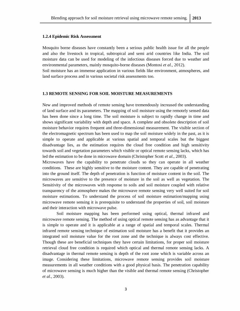
1.3 REMOTE SENSING FOR SOIL MOISTURE MEASUREMENTS
New and improved methods of remote sensing have tremendously increased the understanding
of land surface and its parameters. The mapping of soil moisture using the remotely sensed data
has been done since a long time. The soil moisture is subject to rapidly change in time and
shows significant variability with depth and space. A complete and obsolete description of soil
moisture behavior requires frequent and three-dimensional measurement. The visible section of
the electromagnetic spectrum has been used to map the soil moisture widely in the past, as it is
simple to operate and applicable at various spatial and temporal scales but the biggest
disadvantage lies, as the estimation requires the cloud free condition and high sensitivity
towards soil and vegetation parameters which visible or optical remote sensing lacks, which has
led the estimation to be done in microwave domain (Christopher Scott et al., 2003).
Microwaves have the capability to penetrate clouds so they can operate in all weather
conditions. These are highly sensitive to the moisture content. They are capable of penetrating
into the ground itself. The depth of penetration is function of moisture content in the soil. The
microwaves are sensitive to the presence of moisture in the soil as well as vegetation. The
Sensitivity of the microwaves with response to soils and soil moisture coupled with relative
transparency of the atmosphere makes the microwave remote sensing very well suited for soil
moisture estimations. To understand the process of soil moisture estimation/mapping using
microwave remote sensing it is prerequisite to understand the properties of soil, soil moisture
and their interaction with microwave pulse.
Soil moisture mapping has been performed using optical, thermal infrared and
microwave remote sensing. The method of using optical remote sensing has as advantage that it
is simple to operate and it is applicable at a range of spatial and temporal scales. Thermal
infrared remote sensing technique of estimation soil moisture has a benefit that it provides an
integrated soil moisture value for the root zone and the technique is always cost effective.
Though these are beneficial techniques they have certain limitations, for proper soil moisture
retrieval cloud free condition is required which optical and thermal remote sensing lacks. A
disadvantage in thermal remote sensing is depth of the root zone which is variable across an
image. Considering these limitations, microwave remote sensing provides soil moisture
measurements in all weather conditions with a good physical basis. The penetration capability
of microwave sensing is much higher than the visible and thermal remote sensing (Christopher
et al., 2003).

Blending approach for soil moisture retrieval using microwave remote sensing. 2013
4
As in the study, wet soil medium is in general a mixture of soil particles, air voids, and
liquid water. The water contained in the soil usually is divided into two fractions, bound water
and free water. Bound water refers to the water molecules contained in the first few molecular
layers surrounding the soil particles. The amount of water contained in the first molecular layer
attached to the soil particles is directly proportional to the total surface area of the soil particles
in a unit volume. Electromagnetically, a soil medium is a four component dielectric mixture
consisting of air, bulk soil, bound water, and free water. The complex dielectric constants of
bound and free water are each functions of the electromagnetic frequency, the physical
temperature, and the salinity. The dielectric constant is also a function of the bulk soil density,
the shape of the soil particles, and the shape of the water inclusions (Hallikainen et al., 1985).
The variation of dielectric constant of dry material and that of water is considerably
observable. The dielectric constant of dry soil varies between 2-3 depending upon the texture
whereas the dielectric constant of pure water is around 80 at room temperature and at around 1
GHz. Thus the difference is vividly seen clearly in the case of wet and dry soil. The dielectric
constant is one of the important factors in measuring the soil moisture. The dielectric constant is
an electrical property of matter and is a measure of the response of a medium to an applied
electric field. The dielectric constant is a complex number which contains a real value (ε‘) and
an imaginary (ε‘‘) part. The real part determines the propagation characteristics of the energy as
it passes upward through the soil, while the imaginary part of the constant determines the
energy losses.
1.4 CLASSIFICATION OF MICROWAVE REMOTE SENSING
Measurements in microwave remote sensing of soil moisture broadly follow two distinct
approaches,
1. Employing passive radiometric measurement.
2. Using active backscattering measurement.
Both the approaches have shown a very acceptable and excellent correlation with the soil
moisture content.
However there are significant observable differences in both the approaches of active
and passive microwave remote sensing resulting in differing recommended operating
frequencies for the measurement of the soil moisture parameter. The frequency difference in
microwave remote sensing produces quite a significant difference in the penetration capability.
The commonality in the use of both active and passive microwave remote sensing system in soil
moisture measurement lies in the large disparity between the dielectric constant of water and
dry soil.
1.4.1 Passive Microwave Remote Sensing
The passive microwave remote sensing has shown to be superior for the measurement of soil
moisture at lower frequencies. They are limited to coarser spatial resolution of around 10-30 km
at L-band and C-band respectively. The added advantage is that they have higher sensitivity

Blending approach for soil moisture retrieval using microwave remote sensing. 2013
5
towards soil moisture and less towards the surface geometry. Passive data provide global
monitoring of the earth with a daily temporal sampling which is well suited for various numbers
of applications like NWP models. There are many passive microwave remote sensors for the
measurement of soil moisture as, Advanced Microwave Scanning Radiometer for the Earth
Observation (AMSR-E), Soil moisture and ocean salinity satellite (SMOS),Special Sensor
Microwave Imager (SSM/I), Tropical Rainfall measuring Mission (TRMM), which are
presently operational and providing the satellite data for the globe daily.
1.4.2 Active Microwave Remote Sensing
The active microwave remote sensing system has the capability to provide high spatial
resolution imagery that is in the order to meters to some kilometers, but they lack in higher
temporal resolution. The data is not retrieved daily as in the case of passive sensors. They are in
comparison with passive system, more sensitive to surface roughness, topographic features and
vegetation. Over the vegetation cover, the active microwave data have shown a very good
capability for the discrimination of vegetation type and forest biomass retrieval. Currently, the
active microwave remote sensing through the sensor, Advanced Scatterometer (ASCAT)
onboard MetOp provides soil moisture with higher spatial resolution.
1. 5 BLENDING OF PASSIVE AND ACTIVE MICROWAVE DATA
With varied advantages of active and passive microwave remote sensing individually, soil
moisture is estimated time to time with higher accuracy and improved dataset. Due to higher
needs we combine information derived from both passive and active satellite based microwave
sensors which has the potential to offer improved estimates of surface soil moisture at global
scale (Liu et al., 2011) with higher spatial and temporal resolutions. The enhancement of
information by combining both passive and active microwave products helps in understanding
land surface atmosphere interactions these regions (Liu et al., 2012a). One of the approach used
practically for combining soil moisture derive from active and passive microwave datasets is the
blending approach. Blending is the process of combining two different dataset providing similar
information with different units, scale and resolution, after performing the recalling for the
satellite derived products. It is a method to merge soil moisture estimates from two different
sensors that is from passive and active microwave soil moisture dataset into a single dataset. It
has been done previously by Dr.Yi.Liu from University of New South Wales, Sydney,
Australia, using six sensors. This technique has an added advantage of improved spatial and
temporal soil moisture dataset as compared individually with passive or active soil moisture
product.
1.6 PROBLEM STATEMENT
Various techniques and methods/algorithms have been applied to estimate soil moisture using
the passive and active microwave remote sensing since a very long time with timely
modification of the algorithms for the betterment of the soil moisture values by considering the

Blending approach for soil moisture retrieval using microwave remote sensing. 2013
6
ground parameters and other land and atmospheric parameters which are necessary for precise
soil moisture measurement at defined spatial and temporal resolution.
Active and passive sensors have their own advantages but they have caveats too due to which
the method to estimate soil moisture using only by active or passive is unacceptable. The
present hydrological and climatic modeling techniques demands soil moisture information at
higher spatial as well as temporal scale. The non-availability of higher spatial and temporal
resolution soil moisture data force the researches to relay on model derived soil moisture values
which cannot be validated on global scale due to non-availability of observed data. This gap
area in soil moisture mapping can be bridged through combining the active and passive soil
moisture data products derived using data of various sources (sensors) to enhance the temporal
and spatial resolution.
1.7 RESEARCH OBJECTIVE AND RESEARCH QUESTION
Considering the various above said limitations the major aim of the research is to develop a
technique or an algorithm to estimate soil moisture which has higher spatial and temporal
resolution with acceptable soil moisture values for the particular region. The subsequent
objective is to estimate soil moisture from passive microwave remote sensor, by acquiring the
brightness temperature value from the passive sensor. This is performed to estimate the
quantitative value of soil moisture as per the local conditions prevailing.
1.7.1 Research Objectives
To parameterize the different medium and sensor parameters used in the soil moisture
estimation from passive microwave remote sensing data.
To develop an algorithm for blending the soil moisture products derived from active
and passive remote sensing to obtain higher spatial and temporal resolution.
1.7.2 Research Questions:
How to estimate soil moisture using passive microwave remote sensing and how to
reduce the impediment factors which attenuates the soil moisture estimation?
How to implement blending of soil moisture products derived using microwave that is
active and passive remote sensing data?
Blending approach for soil moisture retrieval using microwave remote sensing. 2013
7
CHAPTER - 2
REVIEW LITERATURE
2.1 INTRODUCTION
Soil moisture defined as, a level of saturation in the upper soil layer relative to the soil field
capacity, and is functioned by rainfall and evapotranspiration. The two parameters have an
important role in the evolution of the soil moisture state and considered significant in the soil
water balance equation too. The soil moisture value is generally expressed in volumetric units
or in percentage. There are various conventional and remote sensing techniques to estimate soil
moisture over the land surface. The microwave remote sensing techniques give large scale
spatially distributed and frequent coverage of the phenomenon and combining that information
with the in-situ measurements provides a quality study of soil moisture.
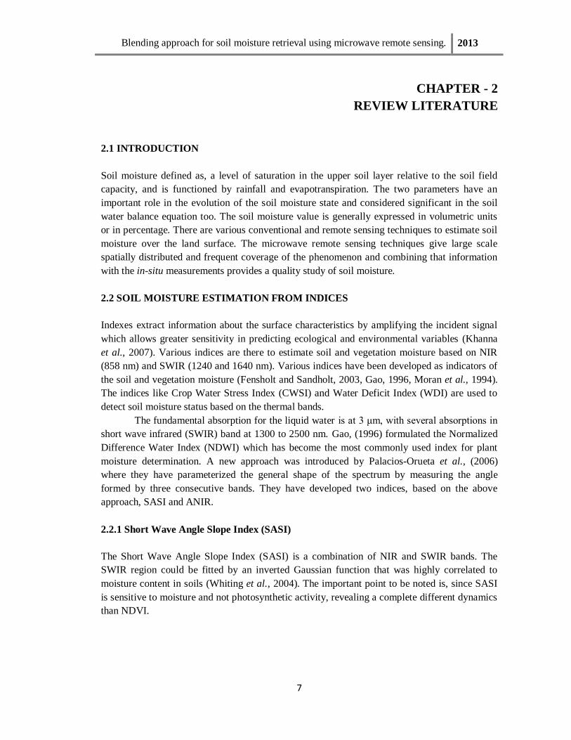
2.2 SOIL MOISTURE ESTIMATION FROM INDICES
Indexes extract information about the surface characteristics by amplifying the incident signal
which allows greater sensitivity in predicting ecological and environmental variables (Khanna
et al., 2007). Various indices are there to estimate soil and vegetation moisture based on NIR
(858 nm) and SWIR (1240 and 1640 nm). Various indices have been developed as indicators of
the soil and vegetation moisture (Fensholt and Sandholt, 2003, Gao, 1996, Moran et al., 1994).
The indices like Crop Water Stress Index (CWSI) and Water Deficit Index (WDI) are used to
detect soil moisture status based on the thermal bands.
The fundamental absorption for the liquid water is at 3 μm, with several absorptions in
short wave infrared (SWIR) band at 1300 to 2500 nm. Gao, (1996) formulated the Normalized
Difference Water Index (NDWI) which has become the most commonly used index for plant
moisture determination. A new approach was introduced by Palacios-Orueta et al., (2006)
where they have parameterized the general shape of the spectrum by measuring the angle
formed by three consecutive bands. They have developed two indices, based on the above
approach, SASI and ANIR.
2.2.1 Short Wave Angle Slope Index (SASI)
The Short Wave Angle Slope Index (SASI) is a combination of NIR and SWIR bands. The
SWIR region could be fitted by an inverted Gaussian function that was highly correlated to
moisture content in soils (Whiting et al., 2004). The important point to be noted is, since SASI
is sensitive to moisture and not photosynthetic activity, revealing a complete different dynamics
than NDVI.

Blending approach for soil moisture retrieval using microwave remote sensing. 2013
8
2.2.2 Angle at NIR (ANIR)
The ANIR is combination of reflectance values in red, NIR, and SWIR bands. The soil
reflectance increases monotonically from visible through SWIR when the soil is dry. The ANIR
has a disadvantage that it is less sensitive to soil moisture level and it is also less a potential tool
for discriminating dry plant matter from soil with multiple-band data. In a greener zone, ANIR
values are smaller than those in dry plant matter or soils and as dry matter content increases
ANIR also decreases. Its range of ANIR is from 0 to 2π radians.
2.2.3 Soil Wetness Variation Index (SWVI)
On the basis of change detection methodology from multi temporal satellite data analysis, a
normalized SWI index called as Soil Wetness Variation Index (SWVI) is formulated, which
decimates the variation related to the different soil water contents and variations determined by
vegetation and roughness effect (Lacava et al., 2005). SWVI is only sensitive to SWI variations,
mainly depending on the soil moisture and not to its absolute values related to the surface
roughness and vegetation cover. The SWI and SWVI are used for an intensive inter-comparison
analysis.
The indices have been a very efficient technique to measure soil moisture and
vegetation effect on that respectively. The indices like NDVI, NDWI, SASI, ANIR, SWVI and
WDI have been widely used to estimate various measures as the amount of vegetation, soil
moisture, and surface conditions. They provide data that is ground dependent and can be used
for calibration and validation purposes.
2.3 GROUND BASED SOIL MOISTURE ESTIMATION METHODS
The ground based techniques involve the soil moisture estimation where the instrument is in
direct contact with soil particles and provides more precise data (Dobriyal et al., 2012). The
point measurements are taken at any time scale by these instruments which can be accurately
calibrated and give depth wise measurements of soil moisture.
2.3.1 Gravimetric Method or Thermostat-Weight Technique
Soil moisture content estimation is done widely by this technique (Schmugge et al., 1980).This
technique involves oven drying a soil sample of known volume at 105οC for 24h. The resultant
water content is calculated by subtracting the oven dry weight from initial field soil weight. The
main advantage of the technique is that it is cost efficient, easy and accurate too. Although the
disadvantage is, it is laborious, time intensive and difficult when soil is rocky (Stafford, 1988).
2.3.2 Neutron Probe Technology
In this instrument, it consists of a probe and an electron counting scalar connected by an
electronic cable. A very high energy, fast moving neutrons are ejected into the soil by a

Blending approach for soil moisture retrieval using microwave remote sensing. 2013
9
radioactive source. The released neutrons are slowed down by the collision with the nuclei of
the hydrogen atoms present in the molecules of water in the soil (Chanasyk and Naeth, 1996).
They are accurate and irrespective of the state of the water. The output from this instrument is
directly linked to the soil moisture. The only limitation is that it is expensive equipment and
requires extensive soil specific calibrations. The depth of the resolution is inadequate, which
eventually makes soil moisture measurement a difficult task.
2.3.3 Tensiometers
It measures the capillary or moisture potential on the basis of suction force exerted on water by
soil (Schmugge et al., 1980). This instrument is cost effective and technique is non-destructive.
It is well capable of measuring the water content in both saturated and unsaturated conditions. It
produces continuous measurement without disturbing the soil. The only limitation is that it is
unsuitable in dry soils and this instrument requires high maintenance because of which it is not
extensively used in the research.
The others ground based soil moisture measuring methods are, time domain
reflectometry, capacitance and frequency domain reflectometry, gypsum block measurements,
pressure plate method, ground penetrating radar method. They all have their own advantages
and disadvantages for measuring soil moisture for different soil type and with different
penetration with varying accuracy.
2.4 MICROWAVE REMOTE SENSING
Microwave remote sensing provides a unique capability for direct observation of soil moisture.
Remote measurements from space provide us the possibility of obtaining frequent, global
sampling of soil moisture over a large fraction of the Earth's land surface. As known,
microwave measurements have the benefit of being largely unaffected by cloud cover and
variable surface solar illumination.
The principle of microwave remote sensing of soil moisture is basically based on the
sensitivity of soil permittivity to the amount of liquid water. The permittivity of a medium, like
moist soil, characterizes electromagnetic wave propagation and attenuation in the medium. The
soil brightness temperature is dependent on the soil permittivity value (Wardlow et al., 2012).
The difference between the dielectric constant of water (about 80 at frequencies below 5 GHz)
and that of dry soil (about 3.5) is very large and significant, due to which the emissivity of soils
varies from approximately 0.6 for wet (saturated) soils to greater than 0.9 for dry soils. These
variations are observed both by passive and active microwave sensors. For a soil at a
temperature of 300 K this variation in emissivity corresponds to a soil brightness temperature
variation of 90 K (Njoku and Entekhabi, 1996). This arises from the tendency of electric dipole
of the water molecule to align itself with the electric field at microwave frequencies (Schmugge
et al., 1993). Various empirical models have been developed in order to provide a relation
between volumetric water content for different soil types to that of dielectric constant at
microwave frequencies (Hallikainen et al., 1985, Dobson et al., 1985).

Blending approach for soil moisture retrieval using microwave remote sensing. 2013
10
2.5 FACTORS INFLUENTIAL IN MICROWAVE REMOTE SENSING
The factors affecting the soil brightness temperature are mainly, soil surface roughness,
attenuation and emission by vegetation cover, surface heterogeneity, some lesser degree to soil
texture and variability in temperature of the soil and vegetation.
The low frequency microwave range of 1-3 GHz that is less than 5 GHz is considered the most
suitable for soil moisture sensing (Jackson et al., 2002). This wavelength is preferred owing to
reduce the atmospheric attenuations and greater vegetation penetration, though it increases the
errors due to radio frequency interferences.
2.5.1 Dielectric Constant
The measurements of dielectric constants as a function of soil moisture have been carried out
over a wide microwave frequency range. The measurements were made for soils with different
texture structures. Two distinct features associated with the relation between the soil dielectric
constant and moisture content has emerged from the study (Spans, 1978).
1) The dielectric constant increases slowly with moisture content and after reaching a
transition moisture value, the dielectric constant increases steeply with moisture content
for all soils.
2) The transition moisture is found to vary with soil type or texture.
2.5.2 Surface Roughness
The surface roughness has a profound effect on the soil moisture. Surface roughness is an
important variable and its knowledge is important for many models too. Roughness parameters
are also very variable in space. For instance, in the agricultural fields where the crops are
grown, the soil surface remain untilled from sowing till the harvest and during this period of
time the surface roughness is assumed to be constant and soil moisture estimation technique is
simplified that is soil moisture variation is a consequence of its dynamics. During the
agriculture inactive period the assumption of constant roughness condition simplifies the soil
moisture estimation. It is important to evaluate the variations of surface roughness occurring
over the growing season and to assess their influence on the estimation of soil moisture from
satellite data (Álvarez-Mozos et al., 2009).
2.5.3 Bulk Density
Soil, bulk density and microwave have a distinct relationship. The microwave emission from
the soil surface reduces as bulk density of soil increases. The increasing bulk density of soil
affects the dielectric properties of dry and moist soil. It has been seen that, dielectric parameters
of soil at microwave frequencies are mainly the function of various properties of soil such as
texture, moisture, bulk density, temperature, and soil type (Gupta and Jangid, 2011).

Blending approach for soil moisture retrieval using microwave remote sensing. 2013
11
2.6 PASSIVE MICROWAVE REMOTE SENSING
Wigneron et al., (2003) have shown a very broad way to retrieve soil moisture considering the
factor of vegetation canopy. The effect of vegetation has to be considered as vegetation absorbs
and reflects part of microwave emission from the soil surface. The three main retrieval
approaches are, statistical techniques, forward model inversion and use of neural networks.
In the statistical approach the land surface information is retrieved by directly manipulating the
measured signals through the empirical relationship as:
Xj = Fj(TB,1,TB,2,….TB,n).
where TB,i corresponds to the sensor configuration and xj is the respective land surface variable.
Statistical method is done based on the classification on dual or multi configuration
observations or the surface soil moisture is statistically related to combination of microwave
emissivity and vegetation indices. The important aspect to be considered here is that, it is a site
specific method which adds to its limitations.
The forward model inversion is used to simulate the microwave radiometric
measurements as a function of land surface characteristics. Here the limitation observed is that,
a prior knowledge of functional form of the process that is to be modeled is needed and multi-
scattering effects are taken into account which further requires large number of inputs.
One of the forward model approach mentioned in the Wigneron et al., (2003) is
statistical inversion approach where the principle is to search for input parameters, consisting of
geophysical parameters that minimizes the squared error between the brightness temperature
measured from satellite data and actual output of the model.
The neural network (NN) method of estimation of soil moisture another widely used
way in remote sensing for the soil moisture estimation. Here, an appropriate set of input-output
data is generated, using the forward model. Then the copy of forward model is made by training
the NN on the set of data. The advantage in this method is that, once the neural network is
trained, parameter inversion can be accomplished quickly.
In Hui Lu et al., (2009) the algorithm developed to retrieve the moisture content is
based on a modified radiative transfer (RT) model, in which the volume scattering measurement
inside the soil layer is calculated through dense media radiative transfer theory (DMRT) (Wen
et al., 1990) and the surface roughness effect is simulated by Advanced Integration Equation
Model (AIEM) (Chen et al., 2003). Using the optimized parameter value, The forward model is
executed to generate the lookup table, which relates the soil moisture content to the brightness
temperature. Then, the soil moisture content is estimated by linearly interpolating the brightness
temperature into inversed lookup table. In this, it has presented the structure of the soil moisture
retrieval algorithm for the space borne passive microwave remote sensing.
Microwave remote sensing offers great possibility of quantifying the surface soil
moisture condition over spatial extent (Champagne et al., 2011). This research examines the use
of surface soil moisture to derive the soil moisture anomaly. Four methods were used to
spatially aggregate information to develop an anomaly. Two methods used soil survey and
climatologically zones to define the region of homogeneity, while the other two methods used
zones defined by data driven segmentation of satellite soil moisture data. This method is used to

Blending approach for soil moisture retrieval using microwave remote sensing. 2013
12
assess the condition of the soil moisture at large spatial scale which can have further
implications like drought assessment etc.
2.7 RELATIONSHIP BETWEEN DIELECTRIC CONSTANT AND VOLUMETRIC
WATER CONTENT
It is very important to understand the relationship between the effective dielectric constant of
the soils and the volumetric water content as it used to determine the soil moisture content.
Various empirical relations have been suggested for the relationship between the dielectric
constant and the vol. water content. The most common one is that of Topp et al., (1980) –
εeff = 3.03 + 9.3θ + 146θ2 – 76.7θ
3
It was suggested that another constant that is, bound water be added with lower dielectric
constant than that of free water as in Dobson et al., (1985).
While the function proposed by Dobson et al., (1984) also takes into account the soil texture by
allowing its coefficients to be dependent on the clay and sand percentages:
εeff = 2.37 + ( - 5.24 + 0.55 x %sand + 0.15 x %clay)θ
+ (146.04 – 0.75 x %sand – 0.85 x %clay) θ2
The models relating the volumetric soil moisture and the dielectric constant are needed in the
study (Peplinski et al., 1995).
The review of all the literature and journals had given the conclusion that passive
microwave remote sensing has the pronounced ability to detect and map the surface soil
moisture due to its penetrating ability and due to its ability to detect the vegetation canopy,
surface roughness and other surface parameters at all weather conditions. The added advantage
of the passive microwave remote sensing for the soil moisture retrieval is that, it provides the
data with good temporal resolution. The data is available on the daily basis and the only demerit
is that of the spatial resolution. The spatial resolution is not so fine; the soil moisture is available
at a coarser resolution and from the top layer only (Christopher Scott et al., 2003)
2.8 ACTIVE MICROWAVE REMOTE SENSING
Several algorithms have been developed to infer the soil moisture using active microwave
remote sensing. The information on multiple radar channels, usually multiple polarization, are
required to separate the effect of surface roughness and surface dielectric constant to extract the
soil moisture information (van Zyl and Kim, 2001). The high sensitivity of active microwave
sensors with respect to soil moisture is the key element in the active microwave remote sensing
(Ulaby and Batlivala, 1976, Ulaby et al., 1978, Dobson and Ulaby, 1986), The backscattering
coefficient (ζο) describes the amount of average backscattered energy compared to the energy of
the incident field. The intensity of ζο is a function of electrical and physical properties of the
target, wavelength, polarization and incidence angle of the radar. Vegetation and surface
roughness are another prominent factors affecting the incident microwave radiation (Barrett et
al., 2009).

Blending approach for soil moisture retrieval using microwave remote sensing. 2013
13
The first-order small perturbation model used to estimate the soil moisture is used to
describe scattering from slightly rough surfaces. Using this model, it is seen that the ratio of the
two co-polarized radar cross section in the linear basis is independent of the surface roughness.
The model has the disadvantage that it is only applicable to smooth surfaces. The first-order
small perturbation inversion will tend to underestimate the surface dielectric constant in the
presence of significant roughness (van Zyl and Kim, 2001).
Based on the algorithm proposed by Oh et al., (1992), they have developed an empirical
model in terms of the RMS surface height, the wave number and the relative dielectric constant.
Here the roughness and the soil dielectric constant are explicitly given in terms of co-
polarization ratio (p) and cross-polarization ratio (q). Expression is developed in terms of
surface dielectric constant from the above said parameters.
Dubois et al., (1995) have developed an empirical model that requires only the
measurement of co-polarized radar cross section, between the frequency 1.5 and 11 GHz to
retrieve mainly surface RMS height and soil dielectric constant from the bare soil. This
algorithm is only applicable to the surfaces with roughness coefficient value less that 3.0 and
angle of incidence to be in between 30ο to 70
ο.
The above said models do not take into consideration the shape of the surface power spectrum
which is related to the surface roughness correlation function and correlation length.
Although, In the algorithm proposed by Shi et al., (1997) the backscattering coefficients
are sensitive to soil moisture, surface RMS height and the shape of the surface roughness
power spectrum.
All the empirical models developed from a limited number of observations might give site
specific results because of the nonlinear response of backscattering to the soil moisture and
surface roughness parameters.
The integrated equation model (IEM) (Fung et al., 1992) which is a physically based
radiative transfer model provides an alternate approach for the retrieval of soil moisture from
the radar data. It is applicable for a wide range of surface roughness conditions; however the
complexity of this model makes it difficult to infer soil moisture and roughness parameter. This
model essentially quantifies the backscattering coefficient as a function of unknown soil
moisture content and surface roughness and known radar configuration.
In the IEM, it is only applicable for single scattering terms where second order scattering is not
considered. Thus for the consideration of multiple scattering terms improved IEM model (Fung
et al., 1996) is applied.
The various complexity and difficulty encountered in the application of theoretical
models has led to the development of the empirical and semi-empirical models (Neusch and
Sties, 1999). The backscattering models have been employed through simple retrieval
algorithms. These types of models have the disadvantage that they are generally derived from
specific data sets, valid only to that area which is under the investigation (Chen et al., 1995).
Here, large databases of study sites are important to ensure that developed models are quite
robust and transferable to other datasets, irrespective of the sensor and surface conditions
(Baghdadi et al., 2008).
The semi empirical models provide a link between the complexity of the theoretical
models and simplicity of the empirical models which may be applied with little information

Blending approach for soil moisture retrieval using microwave remote sensing. 2013
14
about the surface roughness (D‘Urso and Minacapilli, 2006,). The main advantage of these
types of models is that they are site independent – a problem associated generally with
empirical backscattering models.
The most recent technique of soil moisture retrieval is by using polarimetric parameters.
The parameters are coherence, entropy and alpha angle (α). The polarimetric measurements
(Raney, 2007, Dubois-Fernandez et al., 2008) are used to study the dependence of polarimetric
signature on surface parameters such as soil moisture and surface roughness.
The main characteristics of the polarimetric data are that, it allows the discrimination of various
types of scattering mechanisms within an imaged cell. The major advantage is its ability to
measure all the polarization characteristics of the surface.
The study of various literatures on the active microwave remote sensing had provided a
conclusion that the estimation of soil moisture from active microwave remote sensing is a very
profound way of measurement. The added advantage of high spatial resolution is the main
reason to use the active remote sensing. Active microwave remote sensing can be done at any
time irrespective of the atmosphere that is it can be done even if there is no cloud free condition
also (Christopher Scott et al., 2003). The added advantage of this is high sensitivity towards soil
moisture content (Barrett et al., 2009). The only demerit in active microwave remote sensing is
the lower temporal resolution. The data is not available at the daily basis which is a big setback
in the active microwave remote sensor.
2.9 COMBINED ACTIVE AND PASSIVE MICROWAVE REMOTE SENSING
Scatterometer, radar and radiometric responses have often been modeled by separate techniques
individually with satisfactory results. However, a discrete scatter microwave model (Chauhan et
al., 1994) using both active and passive microwave data is used to retrieve the soil moisture
(Chauhan, 1997). The model is according to the established sensor sensitivities to the soil and
vegetation characteristics coupled with emission model to estimate soil moisture. The technique
has been used to determine the optical thickness and RMS height by active remote sensing and
this information is used as ancillary data for inferring soil moisture by passive technique. Here
the determination of the parameters is based on the physically based discrete scatter model and
thereof this technique holds good for all kinds of vegetation and surface conditions. In this
model, the surface roughness inversion algorithm does not require a large database. The main
caveat in this model is that it takes various assumptions into the consideration. The various
assumptions lead to some quantifying error in the estimated value from the parameter which can
only be rectified through ground measurements.
2.10 LEVENBERG-MARQUARDT ALGORITHM
The Levenberg-Marquardt (LM) algorithm is an iterative system that locates the minimum of a
multivariate function that is expressed as the sum of squares of nonlinear real valued functions.
It is one of the standard techniques for nonlinear least-squares problems. The algorithm is
applied to nonlinear least squares minimization.
The function to be minimized is of the form,

Blending approach for soil moisture retrieval using microwave remote sensing. 2013
15
f(x) =
where x = (x1,x2,…,xn) is a vector and rj is the function and it is assumed that m ≥ n.
R can also be defined as:
r(x) = (r1(x), r2(x), …. ,rm(x))
and similarly f can be written as, f(x) =
.
Solving the above equation for the minimum value derives the required parameter estimation.
Nonlinear least squares methods Levenberg-Marquardt (LM) algorithm involves an iterative
improvement to parameter values in order to minimize the sum of the squares of the errors
between the function and the measured data points(Lourakis, 2005, Ranganathan, 2004,
McLauchlan, 2001, Henry, 2011).
This minimization function is used to estimate the soil moisture from brightness
temperature as input and various other parameters required to estimate the value.
2.11 RADIATIVE TRANSFER (RT) METHOD
The important aspect in the radiative transfer method is the interaction between the
radiation from the surface and matter which is explained using two processes, extinction and
emission. The distinction between the two is, if the radiation traversing a medium is reduced in
its intensity it is called extinction, and if medium adds energy of it owns it is defined as
emission. Both the processes occur simultaneously (Ulaby et al., 1981a).
The fundamental quantity in the formulation of the radiative transfer equation is the
specific intensity Iv(r). It is defined in terms of amount of power dP along the direction r within
a solid angle dΩ through an area dA in a frequency interval (v, v + dv) as,
dP = Iv(r) cosθdAdΩ dv
The dimension of Iv is same as that of the spectral brightness. In the remote sensing domain the
radiation at a single frequency is considered. In terms of intensity, the amount of power at a
single frequency is written as,
dP = I(r) cosθdAdΩ.
I(r) is replaced by B for brightness temperature, and the equation governs the variation of
intensities in a medium that absorbs, emits and simultaneously scatters the incident radiation
(Ulaby et al., 1981b).
This algorithm is used to retrieve the land parameters from microwave remote sensing
and specifically used in soil moisture retrievals due to the consideration of various factors and
the preciseness of the value.

Blending approach for soil moisture retrieval using microwave remote sensing. 2013
16
2.12 PRESENT STUDY
Considering the various advantages and disadvantages of the passive and active microwave
remote sensing, where each of which have different sensitivities to soil moisture and vegetation
cover, we have induced a technique to blend the passive and active soil moisture data for a
higher spatial and temporal resolution in the present study. This process preserves the relative
dynamics of the original satellite derived dataset and also establishes a new line of soil moisture
data which has a better resolution for the Indian conditions. It provides the opportunity to
generate a combined product that incorporates the advantages of both microwave techniques
(Liu et al., 2012b, Liu et al., 2011, Wagner et al., 2013a). It moreover enhances the basic
understanding of soil moisture in the water and energy cycle respectively.

Blending approach for soil moisture retrieval using microwave remote sensing. 2013
17
CHAPTER - 3
STUDY AREA AND DATA USED
3.1 STUDY AREA
As discussed in earlier chapters the spatial resolution for which the soil moisture mapping is
done in case of passive microwave remote sensing is of the order 10 to 30 km, hence to analysis
the applicability of any algorithm developed for mapping/estimation of soil moisture using
microwave remote sensing the study area should be of order thousands of square kilometers,
which is a catchment or basin scale in terms of hydrology. Keeping this in mind Ganga River
Basin, the largest river basin in India has been chosen as study area for present study. The
location map of Ganga River Basin is shown in Fig. 3.1
Fig. 3.1: Study Area

Blending approach for soil moisture retrieval using microwave remote sensing. 2013
18
The Ganga basin extends its vast stretch over an area of 9,26,080.3734 sq. km, ranks among the
largest in the world in drainage basin area and length and it primarily lies in India with Tibet,
Nepal and Bangladesh as the other parts where Ganga basin touches, and the extent from
22.625ο to 31.375
ο North and 73.375
ο to 88.8750
ο East. The basin is bounded on the north by
the Himalayas, on the west by the Aravallis and the ridge separating it from Indus basin, on the
southern part by the Vindhyas and Chhota nagpur plateaus and on the east by the Brahmaputra
ridge. The outlet of the Ganges basin is considered at the Farakka barrage (24.80ο N and 87.93
ο
E).
The river has two main headwaters in the Himalayas - the Bhagirathi and the Alaknanda
and others for each of its other tributaries. The Bhagirathi flows from the Gangotri glacier at
Gomukh and the latter from a glacier near Alkapuri. Farther downstream, the river is joined by a
number of other Himalayan rivers, the Yamuna, Ghaghara, Gomti, Gandak and Kosi. However,
the Ganga and its major tributaries, the Yamuna, Ram Ganga, and Ghaghara are the only
Himalayan rivers that have significant base and flood flows.
The basin engulfs semi-arid valleys in the rain shadow north of the Himalaya, densely
forested mountains south of the highest ranges, the scrubby Shiwalik foothills and the fertile
Gangetic Plains. Central highlands south of the Gangetic Plain have cloud touching plateaus,
hills and mountains intersected by valleys and river plains. The annual surface water potential
of the basin has been assessed as 525 km³ in India, out of which 250 km³ is utilizable water.
There is about 5,80,000 km² of arable land, 29.5% of the cultivable area of India (Source:
Ganga basin, Wikipedia).
The basin lies in the States of Uttar Pradesh, Madhya Pradesh, Bihar, Rajasthan, West
Bengal, Haryana, Himachal Pradesh and the Union Territory of Delhi.
3.1.1 PHYSIOGRAPHY
The main physical sub-divisions are the Northern Mountains, the Gangetic Plains and the
Central Highlands. Northern Mountains includes the Himalayan ranges comprising their foot
hills. The Gangetic plains, situated between the Himalayas and the Deccan plateau, constitute
the most fertile plains of the basin which is perfectly suited for intensive cultivation. The
Central highlands lying to the south of the Great Plains consists of mountains, hills and plateaus
intersected by valleys and river plains. They are largely covered by forests. Aravali uplands,
Bundelkhand upland, Malwa plateau, Vindhyan ranges and Narmada valley lie in this region.
3.1.2 SOIL TYPE
Predominant soil types found in the basin are sandy, loamy, clay and their combinations such as
sandy loam, loam, silty clay loam and loamy sand soils. The cultivable area of Ganga basin is
about 57.96 M.ha which is 29.5% of the total cultivable area of the country (Source: Central
Water Commission (CWC), India).

Blending approach for soil moisture retrieval using microwave remote sensing. 2013
19
3.1.3 River System
The Ganga originates as Bhagirathi from the Gangotri glaciers in the Himalayas at an elevation
of about 7010 m in Uttarkashi district of Uttarakhand and flows for a total length of about 2525
km up to its outfall into the Bay of Bengal through the former main course of Bhagirathi-
Hooghly (Source: Central Water Commission (CWC), India). The principal tributaries joining
the river are the Yamuna, the Ramganga, the Ghaghra, the Gandak, the Kosi, the Mahananda
and the Sone. Chambal and Betwa are the two important sub-tributaries. Click for basin map of
the sub-basin showing the river system and other features.
3.1.4 Climate and Hydrology
The water supply in the Ganga basin depends partly on the rains brought by the south westerly
monsoon winds from July to October, and on the flow from melting Himalayan snows in the hot
season from April to June. Precipitation in the river basin accompanies the southwest monsoon
winds, but it also comes with tropical cyclones that originate in the Bay of Bengal between June
and October. Only a small amount of rainfall occurs in December and January. The average
annual rainfall varies from 762 mm at the western corner of the basin to more than 2,290 mm at
the eastern. In the upper Gangetic Plain in Uttar Pradesh, rainfall averages about 760-2290 mm
whereas in the Middle Ganges Plain of Bihar, from 1016 to 1524 mm and in the delta region,
between 1524 and 2540 mm. The delta region experiences strong cyclonic storms both before
the commencement of the monsoon season, from March to May, and at the end of it, from
September to October.
3.1.5 Important Projects
The Ganga and Yamuna canal systems irrigate vast areas utilizing the perennial flow of the
river. Important storages constructed in the basin include Matatila, Sarda Sagar, Ramganga,
Mayurakshi reservoirs. Some other important projects are Rajghat on Betwa, Bansagar on Sone
and Tehri on Bhagirathi. The hydropower potential of the basin is 10,715 MW at 60% load
factor.
3.1.6 Mythological Scenario
The Ganga basin is the cradle of Hindu and Buddhist pilgrimage culture. Some of the most
important centers of spiritual learning and healing have thrived for centuries along the Ganges
banks. At the headwaters of the Ganga in the Himalayas, sacred shrines at Tapavan, Gomukh,
Bhojbasa, and Gangotri mark the sources of illumination. The shrines of Kedarnath and
Badrinath also celebrate their position in the upper reaches of the watershed and considered the
important shrines of India and Indian culture preserving the deepest heritage of India. Farther
downstream in the Himalayas are Uttarkashi and Rishikesh and along the plains lie Haridwar,
Allahabad (Prayag), Banaras, Vindhyachal, Nadia and Kalighat. Along the river Yamuna, there
are sacred places of Mathura and Vrindavan are located and inland within the Ganga basin, the

Blending approach for soil moisture retrieval using microwave remote sensing. 2013
20
Hindu center of Vindyachal and the Buddhist sites of Gaya, Rajgir and Nalanda. In these
pilgrimage centers and in countless other smaller sacred spots along her great traverse, pilgrims
worship the Ganga and carry away her pure water for worship and purification.
3.2 DATA USED AND DATA PROPERTIES
The various satellite products used in the study are AMSR-E and ASCAT soil moisture product,
GLDAS-Noah modeled soil moisture product. The data is chosen for the year 2009 as the
AMSR-E has discontinued providing the soil moisture data after October 2010 and
simultaneously ASCAT and Noah data is retrieved for the year 2009 only. AMSR-E soil
moisture product is preferred for the present research work due to the following reasons:
1. AMSR-E sensor works at the frequency of 6.9 GHz and the Soil Moisture Ocean
Salinity mission (SMOS), providing the soil moisture data too operates at the frequency
of 1.4 GHz at which radio frequency interference (RFI), Faraday rotation and galactic
noise become increasingly significant and is the main sources of error (Njoku and
Entekhabi, 1996). Thus AMSR-E is preferred in this study.
2. The algorithm to retrieve soil moisture by using brightness temperature (Tb) of AMSR-
E is less complex and in the algorithm it considers all the parameters related and
required to estimate soil moisture and surface roughness, whereas SMOS algorithm is
more complex and needs much understanding.
3. ASCAT sensor is chosen as the active sensor for the soil moisture which operates at the
frequency of 5.3GHz (C-band) and this is closer to the frequency in which AMSR-E
operates too, whereas SMOS operates at 1.4 GHz that is in L-band due to which it is not
chosen for the present research.
4. A model data is needed for the rescaling purpose in the blending process and from
various GLDAS models, mosaic, Community Land Model (CLM), VIC and Noah,
Noah is considered best because of its similar spatial resolution as that of ASCAT, as
accordingly AMSR-E is chosen having same spatial resolution as that of Noah land
surface model.
Noah model is preferred as this model and VUA-NASA algorithm in AMSR-E uses a common
soil property dataset (soil map by FAO). Indian Meteorological department (IMD) district wise
rainfall data has also been taken from India Water Portal, to establish a correlation and analysis
with the soil moisture. Temperature data have been taken from, National Oceanic and
Atmospheric Administration - National Climatic Data Center (NOAA – NCDC) which is used
in the analysis and comparison with the soil moisture. Ganga basin has been delineated from the
DEM derived from GTOPO with spatial resolution of 1 km.

Blending approach for soil moisture retrieval using microwave remote sensing. 2013
21
3.2.1 Advanced Microwave Scattering Radiometer – Earth Observation (AMSR-E)
Advanced Microwave Scattering Radiometer on-board Aqua is a twelve channel, six frequency
total power passive microwave radiometer system. The data has been retrieved globally from
National Snow and Ice Data center (NSIDC). It measures brightness temperatures at 6.925,
10.65, 18.7, 23.8, 36.5, and 89.0 GHz as in Table 3.1. Vertically and horizontally polarized
measurements are taken at all channels. Aqua is one of a series of space based platforms that are
central to NASA's Earth Science Enterprise (ESE), a long-term study of the scope, dynamics
and implications of global change. The primary focus for the Aqua Project is the multi-
disciplinary study of the Earth's Interrelated Processes (atmosphere, oceans, and land surface)
and their relationship to earth system changes. It allows long-term change detection, identify its
human and natural causes and advance the development of models for long-term forecasting
(Source: AMSR-E Data Users Handbook, 4th Edition, March 2006,)
AMSR-E scans the Earth‘s surface by mechanically rotating the antenna and acquires
radiance data of the Earth‘s surface. The aperture diameter of AMSR-E antenna is 1.6 m, and its
spatial resolution is about 5 km in the 89 GHz band and about 60 km in the 6.9 GHz band of the
largest wavelength. It conically scans and keeps an angle of incidence on the earth surface (55
degrees) to be constant and minimizes the effect of sea surface wind on the sea surface
temperature and accomplishes a swath width of about 1450 km. Further, AMSR-E has a
function to acquire radiance temperatures of deep space (about 2.7 °K) for calibrating
observation data and high temperature calibration source.
Table 3.1: AMSR-E Main Characteristics
(Source: AMSR-E Data Users Handbook, 4th Edition, March 2006).

Blending approach for soil moisture retrieval using microwave remote sensing. 2013
22
AMSR-E measures geophysical parameters supporting several global change sciences and
monitoring efforts as shown in Table 3.2.
Table 3.2: Observation Targets and Purpose of AMSR-E
(Source: AMSR-E Data Users Handbook, 4th Edition, March 2006).
a) Temporal Coverage
Temporal coverage is from 19th June 2002 to 3
rd October 2010.
Each swath spans approximately 50 minutes. The data sampling interval is 2.6 m sec per sample
for the 6.9 GHz to 36.5 GHz channels, and 1.3 m sec for the 89.0 GHz channel. A full scan
takes approximately 1.5 seconds. AMSR-E collects 243 data points per scan for the 6.9 GHz to
36.5 GHz channels, and 486 data points for the 89.0 GHz channel. The number of satellite
passes per day is a function of latitude as shown in AMSR-E Observation Times.
b) Spatial Coverage
Spatial Coverage Map of AMSR-E is shown in Fig. 3.2.This map shows a typical day of
coverage with 28 half-orbits.

Blending approach for soil moisture retrieval using microwave remote sensing. 2013
23
Fig. 3.2: Spatial Coverage of AMSR-E (Source: NSIDC)
Coverage is global between 89.24°N and 89.24°S, except for snow-covered and densely-
vegetated areas. The swath width is 1445 km.
b.1) Spatial Resolution
Input brightness temperature data at 10.7 GHz, corresponding to a 38 km mean spatial
resolution, are re-sampled to a global cylindrical 25 km EASE-Grid cell spacing. The effective
spatial resolution is thus slightly higher than the inbuilt 38 km resolution (Source: NSIDC).
b.2) Grid Description
Level-2A brightness temperatures are re-sampled to a global cylindrical EASE-Grid (1383
columns by 586 rows) with a nominal grid spacing of 25 km (true at 30°S). In the case of the
Level-2B soil data, each geophysical variable value has a corresponding EASE-Grid row and
column index (Source: NSIDC).
3.2.2 Advanced Scatterometer (ASCAT)
The Advanced Scatterometer (ASCAT) onboard MetOp is an active microwave remote sensing
instrument that was designed EUMETSAT, with high radiometric accuracy, and its multiple-
viewing capabilities to make it an attractive sensor for measuring soil moisture (Wagner et al.,
2013b). The data have been provided by Integrated Climate Data center (ICDC). In ASCAT the
incidence angle range is extended to 25°–65°. ASCAT covers two 550 km swaths separated by
approximately 360 km from the satellite ground track. It uses two sets of three antennae, one on
each side of the satellite ground track.
The ASCAT Level 2 soil moisture products are generated and distributed in near real
time. The main geophysical parameter derived from ASCAT data is soil moisture index, which
represents the degree of saturation of the topmost soil layer (< 5 cm) and is given in percent,

Blending approach for soil moisture retrieval using microwave remote sensing. 2013
24
ranging from 0 (dry) to 100 (wet). Level 2 soil moisture products are generated by European
Organization for the exploitation of Meteorological Satellites (EUMETSAT) using the so-called
Water retrieval package (WARP-NRT) software, originally developed by the Institute of
Photogrammetry and Remote Sensing of the Vienna University of Technology, based on the
L1b averaged products on 12.5 and 25 km swath grids, as well as on a long term historical
database of geo-located scatterometer soil moisture values around the globe.
ASCAT is indeed a suitable sensor for soil moisture retrieval for various reasons, its
operation frequencies of 5.3 GHz is in the range of microwave frequencies (< 10 GHz) where
the inclusion of liquid water to soil content strongly increases the soil dielectric constant.
Therefore, when the soil moisture content increases, so does the dielectric constant at the air-
soil boundary and therefore the backscatter value. This dependence of the backscattering
intensity on the soil moisture content implies that ASCAT backscatter (ζο) measurements
provide a relatively direct measurement of the soil moisture content over bare soils. In the
presence of vegetation, the value of ζο changes, making it vital to correct the model or
algorithm considering the effect of vegetation on the overall backscatter. Even, the roughness
factor has an important effect on the backscatter measurements (Wagner et al., 2013b). Fig 3.3
shows the ascending and descending pass of ASCAT sensor.
Fig. 3.3: ASCAT Soil Moisture Index (Ascending Pass) (Source: ASCAT Factsheet,
EUMETSAT)

Blending approach for soil moisture retrieval using microwave remote sensing. 2013
25
Fig. 3.4: ASCAT Soil Moisture Index (Descending Pass) (Source: ASCAT Factsheet,
EUMETSAT)
The Fig 3.3 & 3.4 shows soil moisture index values derived from ASCAT on MeTop during
October 10th
, 2010 for ascending and descending passes respectively. The operational
generation and dissemination of these products has started in December 2008 by Vienna
University of Technology. The grid spacing of this ASCAT soil moisture product is 25 km,
covering the two ASCAT swaths, which are each 550 km wide and are located at a distance of
approximately 350 km on either side of the sub-satellite ground track (Source: ASCAT
Factsheet, EUMETSAT).
3.2.3 Global Land Data Assimilation System – Noah (GLDAS-Noah)
Land surface temperature and wetness conditions affect and also get affected by numerous
climatological, meteorological, ecological and geophysical phenomena. It is important to derive
accurate, high-resolution estimates of terrestrial water and energy storages as these variables are
very vital for predicting climate change and for executing wide array of studies in ecological
and environmental studies. Furthermore, since soil moisture, temperature, and other necessary
parameters are location based induces errors in the representation of these in different climate
models and thus it leads to incorrect predictions. The discrepancies are also generated due to
biases in the land surface forcing data and parameterization.
Thus, a Global Land Data Assimilation System (GLDAS) has been developed jointly by
scientists at NASA, GSFC, NOAA to make use of new generation of ground based and space-
based observation systems. The data is taken from Goddard Earth Science Data and Information
Services center (GES DISC). In the GLDAS model, the constraints are applied in two ways that
is, by forcing the land surface models (LSMs) with observation based meteorological fields and
by employing data assimilation techniques.

Blending approach for soil moisture retrieval using microwave remote sensing. 2013
26
Table 3.3: GLDAS Forcing and Output Field Information.
(Source: Rodell et al., 2004)
GLDAS comprises of land surface model that is, National centers for Environmental
Prediction/Oregon State University/ Air Force/ Hydrologic Research Lab Model (Noah) which
provides a temporally and spatially consistent characterization of the hydrological cycle.
GLDAS model derived estimates are mainly 3-hourly products with 0.25ο spatial resolution,
while satellite based observations offer twice-daily instantaneous retrievals at similar spatial
scales (Liu.Y.Y et al., 2009). The GLDAS forcing and output field information is provided in
Table 3.3.
The fine scale variability of the observation based precipitation is reflected in the fines
scale patterns of soil moisture in the derived forcing run because soil moisture shows a high
degree of variability at all scales (Famiglietti et al., 1999). The fine scale soil moisture
variability is evident in the derived forcing run results. This may be preferable from a weather
forecasting perspective. However, the broader patterns of soil moisture are not necessarily
more accurate in the derived forcing run.
While, deriving the soil moisture content map, porosity and the percentages of sand, silt
and clay were horizontally re-sampled to the 0.25ο GLDAS grid and interpolated to 0-2, 2-150,
150-350 cm depths from the original depths. These depths were chosen as to facilitate future
assimilation of surface soil moisture fields derived from AMSR-E satellite measurements.
GLDAS is a global, high resolution terrestrial modeling system that incorporates both satellite
and even ground based observations to generate optimal fields of land surface states and fluxes
in real time (Rodell et al., 2004).

Blending approach for soil moisture retrieval using microwave remote sensing. 2013
27
3.2.4 Ground Soil Moisture Data
The ground (in-situ) soil moisture data is taken from International Soil Moisture Network
(ISMN) for the China location, as the ground data for the Indian region was unavailable for the
present time period chosen. The MAQU network in China consisting of 20 ground stations
located at the eastern edge of the Tibetan plateau in central China at an average altitude of
3000m MSL. Out of the 20 stations in the network, the most suitable was CST-02 located at
latitude 33 40‘N and longitude 102 09‘E at 3449m MSL with dominant land class as grass. The
soil moisture is measured at the depth of 5 cm using ECH20 EC-TM (Tenshiometer). The
ground soil moisture measured at 5:00 am is taken for the validation purpose.

Blending approach for soil moisture retrieval using microwave remote sensing. 2013
28
CHAPTER - 4
METHODOLOGY
4.1 INTRODUCTION
The methodology implied in this research work mainly focuses on the blending of soil moisture
data acquired from the passive and active microwave dataset, using a reference dataset having
same spatial and temporal resolution as that of the microwave data. The methodology also
involves the retrieval of soil moisture from the brightness temperature (Tb) data observed
through passive microwave remote sensing. Fig 4.1 represents the overall flowchart of the
methodology.
Fig. 4.1: Flow Chart Depicting the Overall Methodology

Blending approach for soil moisture retrieval using microwave remote sensing. 2013
29
The methodology is mainly divided into following sections:
1. Acquiring the required datasets for the study time period.
2. Preparation and preprocessing of the datasets for the study area.
3. Retrieval of soil moisture from the passive microwave data.
4. Cumulative distribution function matching approach for rescaling.
5. Blending the microwave dataset all together.
4. 2 DATA ACQUISITION AND SOFTWARE USED
The primary data acquired is the soil moisture data for the time period 01st January 2009 to 31
st
December 2009 i.e., for a complete one year time span, from various sensors and sources for the
purpose of blending. The dataset is classified according to the type of microwave sensor and the
selected reference data.
4.2.1 Satellite Data Acquired
a) AMSR-E data
The passive microwave data is acquired from Advanced Microwave Scanning Radiometer -
Earth Observing System Sensor on the NASA‘s Aqua Satellite for the year of 2009. The Level-
2B land surface product (AE_Land) of AMSR-E includes daily measurements of surface soil
moisture, vegetation/roughness water content interpretive information, and quality control
variables. Ancillary data includes time, geolocation, and quality assessment. Input brightness
temperature data at 10.7 GHz, corresponding to a 38 km mean spatial resolution, are re-sampled
to a global cylindrical 25 km Equal-Area Scalable Earth Grid (EASE-Grid) cell spacing. The
data is acquired from National Snow and Ice data Centre (http://nsidc.org/data/amsre/). The data
is in the units of m3 / m
3.
b) ASCAT data
The Advanced Scatterometer onboard MetOp provides the active microwave data from its
scatterometer sensor. The data is acquired in two forms, image form and the non-image form.
I. Image form: The image form of the ASCAT data for the Indian region is received
from Integrated Climate Data Centre (ICDC), CliSAP/Klima Campus, University of
Hamburg, Hamburg, Germany on request basis. The soil moisture data is available
as 5-Day composites for the year 2009 at 25 km spatial resolution.
II. Non-Image form: The non-image form of data is acquired from Institute of
Photogrammetry and Remote Sensing (IPF), Vienna Institute of Technology (TU
Wien), Vienna, Austria from Dr. Wolfgang Wagner, for the time duration 01
January 2007 to 31 May 2012. The data is in the form of discrete global grid
(DGG). The grid is defined such that the spacing is approximately 12.5 km. The
total grid consists of 32,64,391 points, where 8,39,826 points are defined over the
land. The grid is sub-divided globally into 2,592 cells which cover 5ο X 5
ο each.

Blending approach for soil moisture retrieval using microwave remote sensing. 2013
30
The data is in the units of percentage that is from 0-100%. Fig 4.2 gives the basic
idea of the cells with their index and number of grid points contained in it (Product
Sheet: ASCAT Surface Soil Moisture 25 km Time Series).
Fig. 4.2: Cell Structure of Discrete Global Grid (DGG) (Source: TU Wein University, ASCAT
soil moisture product).
c) GLDAS-Noah Data
The Global Land Data Assimilation System (GLDAS) - Noah land surface model data product,
version 1 with 3-h time interval and 0.25ο spatial resolution. The data is acquired for the entire
year 2009. Noah model uses a four-layered soil description with a 10-cm thick top layer and
takes into account the fractions of sand and clay. Out of the four layered soil moisture value
provision, the value of the top layer that if for 0-10 cm soil moisture value is taken into
consideration in the research. The data is in the units Kg / m2. The data is acquired from the
open portal, Goddard Earth Sciences Data and Information Service Center (GES DISC),
(http://disc.gsfc.nasa.gov/hydrology/data-holdings).

Blending approach for soil moisture retrieval using microwave remote sensing. 2013
31
4.2.2 Software Used
The software packages and programming languages used to complete this study are listed
below,
ERDAS Imagine 9.3
Arc GIS 10.0
ILWIS 3.3
ENVI 4.3
IDL 6.3
Panoply 3.1.8
4.3 PREPARATION AND PREPROCESSING OF THE DATASETS
The dataset acquired from passive microwave remote sensor that is AMSR-E is first extracted
for the study area and then multiplied with the scale factor 0.001 (National Snow and Ice Data
Center, Detailed data description) to acquire the true value of soil moisture. The soil moisture
data and brightness temperature is available at 6.9 GHz for horizontal and vertical polarization
in ascending and descending mode. The data at both modes are averaged to finally get the
required soil moisture and brightness temperature value at 6.9GHz frequency.
The image form of ASCAT data was available in Network Common Data Form
(NetCDF) i.e. .nc format which has to be converted to compatible image format specifically
either in .img (Image format) or .tiff (tagged information file format) format which has to be
further processed. The conversion was done with the aid of customized code developed in
Python 2.7 programming language (Annexture-1). The data is then extracted for the study area
by masking it with the vector layer (shape file) of the Ganga basin.
The GLDAS-Noah data is a combination of various parameters providing information
of various land variables. There are total 22 geophysical parameters subsisted in the GLDAS
data set. The Noah data too was in .nc (NetCDF) format which is again converted to the image
format by specifically extracting only the soil moisture data out of total parameters available.
The soil moisture data is available for four different depths, out of which the extraction is
performed for the top most layer (0-10 cm) only as the AMSR-E soil moisture data also
represents the top 0-5 cm layer only. The soil moisture dataset is again extracted by mask to
retrieve data for the study area.
The original unit of Noah soil moisture data is kg/m2 which has to be converted to
m3/m
3, so that it would be similar with the AMSR-E data units. The conversion is done by
considering the top soil layer depth as 10 cm.
During the preprocessing, it is important to make sure that all the data set has same
spatial extent, similar row and column number that mean same cell size and similar projection
system. Due to the voluminous data, the extraction and conversion from .nc to image format has
been done using programming in Python language. Coding was performed in Python 2.7.3 and
2.6.5 programming language using Arcpy and GDAL modules.

Blending approach for soil moisture retrieval using microwave remote sensing. 2013
32
All the above mentioned dataset have snow covered area in the upper reaches of Ganga basin,
the snow cover have to removed by masking it with the snow extent provided by the MODIS
data for the year 2009, as presence of soil moisture over the snow area is not acceptable.
4.4 RETRIEVAL OF SOIL MOISTURE FROM THE PASSIVE MICROWAVE DATA
The retrieval of soil moisture from passive microwave sensor using the brightness temperature
is the main task and the algorithm flow chart depicting the same is given in Fig. 4.3,
Fig. 4.3: Flow Chart Depicting Soil Moisture Retrieval Using Passive Microwave Data
The retrieval algorithm for soil moisture (me) uses a physically-based radiative transfer model
(Njoku, 1999) and for the estimation of soil moisture the Te and We values needs to be
calculated. The baseline algorithm (AMSR Land Surface Parameters, Algorithm Theoretical
basis document version 3.0, Eni G. Njoku) used in present study uses the two lowest AMSR
frequencies (6.9 and 10.7 GHz) as the Surface roughness and vegetation scattering effects
increasing complexity above ~10 GHz, and the uncertainty in derived products is greater above
~10 GHz. These frequencies also have better vegetation penetration and soil moisture sensitivity
though with the decreased spatial resolution.

Blending approach for soil moisture retrieval using microwave remote sensing. 2013
33
In general parameter retrieval algorithms the land surface is modeled as absorbing vegetation
layer above soil in Fig 4.4.
Fig 4.4: Model Representation of a Space-Borne Radiometer, viewing a heterogeneous earth
surface (Njoku, 1999)
The brightness temperature TBp observed at the top of the atmosphere at a given incidence
angle and at a given frequency can be expressed by the radiative transfer equation (Njoku,
1999).
TBp = Tu + exp (-ηa) [{Td rsp exp (-2ηc)} + {esp Ts exp (-ηc) +
Tc (1 - ηp) [1 – exp (-ηc)] [1 + rsp exp (-ηc)]}] - [1]
where,
Tu - Upwelling atmospheric radiation (watt/m2).
Td - Downwelling atmospheric radiation (watt/m2).
Ta - Atmospheric Opacity.
Tc - Vegetation temperature (K).
ηc - Vegetation opacity.
rsp - Soil reflectivity.
Ts – Effective soil temperature (k).
ωp – vegetation single scattering albedo.
The assumption in the above equation is that, a specular soil surface with no reflection at air-
vegetation boundary.
Another simplifying approximation is that the vegetation and underlying soil are at
close to the same physical temperature Te. This approximation does not degrade the moisture
retrieval accuracy, but will result in the retrieval of a mean or effective radiating temperature of
the composite soil/vegetation medium.

Blending approach for soil moisture retrieval using microwave remote sensing. 2013
34
Substituting Ts ≈ Tc = Te in Equation (1) we obtain:
TBp = Tu + exp (-ηa) [{Td rsp exp (-2ηc)} + Te {(1 - rsp) exp (-ηc) + (1 - ωp)
[1 - exp (-ηc)] [1 + rsp exp (-ηc)]}] - [2]
Atmosphere as the parameter -
The expressions for Tu and Td are obtained from the literature (Hofer and Njoku, 1981).
Tu and Td can be expressed using the effective radiating temperature approximation as;
Tu ≈ Td ≈ Tae [1 - exp (-ηa)] - [3]
where, Tae is the mean temperature of the microwave-emitting region of the atmosphere. This
expression is valid for most atmospheric water vapor and cloud conditions. Tae is frequency
dependent and also depends on the distributions of temperature, humidity, and liquid water. Tae
may be expressed simply as a function of the surface air temperature Tas and a frequency
dependent offset δTa:
Tae ≈ Tas - δTa - [4]
The effect of uncertainty in Tae on the observed TBp is sufficiently small. The opacity ηa along
the atmospheric path is dependent on the viewing angle q and the precipitable water qv and
vertical-column cloud liquid water ql. It can be expressed as:
ηa = (to + av qv + al ql ) / cosθ - [5]
where, ηo is the oxygen opacity at nadir, and av and al are frequency-dependent coefficients.
Values for these coefficients are derived for water vapor and droplet absorption in the
atmosphere (Rayleigh absorption is assumed for the cloud droplets) from various literatures and
journals (Njoku and Li, 1999).
Surface as the parameter -
The dependence of ηc on vegetation columnar water content follows an approximately linear
relationship, written as (Njoku, 1999):
ηc = b we / cosθ - [6]
where, cosθ accounts for the slant path through the vegetation. The coefficient b depends on
canopy structure and frequency. Theory and experimental data suggest that for given vegetation
type (b,) is approximately proportional to frequencies below ~10 GHz (Jackson and Schmugge,
1991, Le Vine and Karam, 1996).
This indicates that at higher frequencies the frequency dependence of b decreases and
its dependence on canopy structure eventually increase. This provides rationale for restricting
the physically-based retrieval algorithm to be in between 6.9 and 10.7 GHz.
The reflectivity of rough soil, rsp, is related to that of smooth soil rop, by the semi-empirical
formulation (Njoku and Li, 1999),

Blending approach for soil moisture retrieval using microwave remote sensing. 2013
35
rsv = [(1 - Q) rov + Q roh ] exp (-h) - [7]
rsh = [(1 - Q) roh + Q rov ] exp (-h) - [8]
Expression for h and Q are:
Q = 0.35[1 – exp (-0.6.ζ2.λ)] - [9]
h =
- [10]
where, λ is frequency of radiometer and ζ is the surface rms height.
The Fresnel expressions relate the reflectivities rov and roh of a smooth, homogeneous soil to the
complex dielectric constant of the soil er:
rov =
- [11]
roh =
- [12]
From the above equation, θ is the incidence angle relative to the surface normal. For a given
frequency, the dielectric constant depends on the volumetric soil moisture content me and to a
lesser extent on soil type.
This relationship can be expressed as:
εr = f (me ; ρb, s, c) - [13]
The most common one is that of Topp et al., (1980) providing the relationship between the
effective dielectric constant and soil moisture is –
εeff = 3.03 + 9.3θ + 146θ2 – 76.7θ
3 - [14]
While the function proposed by (Dobson et al., 1984) takes into account the soil texture by
allowing its coefficients to be dependent on the clay and sand percentages:
εeff = 2.37 + ( - 5.24 + 0.55 x %sand + 0.15 x %clay)θ
+ (146.04 – 0.75 x %sand – 0.85 x %clay) θ3 - [15]
The high sensitivity of brightness temperature to soil moisture is the principal advantage of
using microwave radiometry for soil moisture sensing (Njoku, 1999).
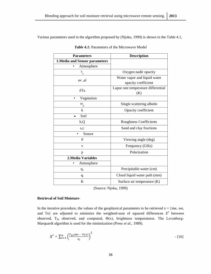
Blending approach for soil moisture retrieval using microwave remote sensing. 2013
36
Various parameters used in the algorithm proposed by (Njoku, 1999) is shown in the Table 4.1,
Table 4.1: Parameters of the Microwave Model
(Source: Njoku, 1999)
Retrieval of Soil Moisture-
In the iterative procedure, the values of the geophysical parameters to be retrieved x = {me, we,
and Te} are adjusted to minimize the weighted-sum of squared differences X2 between
observed, TBi observed, and computed, Ф(x), brightness temperatures. The Levenberg-
Marquardt algorithm is used for the minimization (Press et al., 1989).
X2 =
–
- [16]
Parameters Description
1.Media and Sensor parameters
• Atmosphere
ηo Oxygen nadir opacity
av ,al Water vapor and liquid water
opacity coefficient
δTa Lapse rate temperature differential
(K)
• Vegetation
ωp Single scattering albedo
b Opacity coefficient
Soil
h,Q Roughness Coefficients
s,c Sand and clay fractions
• Sensor
θ Viewing angle (deg)
v Frequency (GHz)
p Polarization
2.Media Variables
• Atmosphere
qv Precipitable water (cm)
ql Cloud liquid water path (mm)
K Surface air temperature (K)

Blending approach for soil moisture retrieval using microwave remote sensing. 2013
37
At each retrieval point, the algorithm starts with a-priori values of the geophysical variables xo
and adjusts these iteratively until X2 convergence to the minimum value of less than 1. ζi
represents the measurement noise in channel i. The model Ф(x) is mathematically sound and
hence convergence is normally fast, except where the model cannot adequately represent the
surface emission, or where the sensitivity to the parameters is too low. The atmospheric
variables of the model qv, ql, Tas, and δTa are given an initial values derived from climatology.
The atmospheric parameters to, av, and aw, are known constants. The parameters b, h, Q, ωp, ρb,
s, and c are given fixed values based on the model.
This algorithm is applied in present study to estimate the soil moisture from the
brightness temperature considering various surface and atmospheric parameters and basic
The soil moisture retrieved from the passive microwave sensor (AMSR-E) lacks the spatial
resolution i.e. coverage of many areas is lacking due to the sensor orbit and the swath width. To
overcome this limitation it is combined with the active sensor (ASCAT) keeping the GLDAS-
Noah as the reference. Rescaling is performed for both AMSR-E and ASCAT as the spatial
extent, scale and units are not common and rescaling is done to get the data in a similar format
as that of the refereed data chosen.
4.5 CDF MATCHING APPROACH
This section describes the process of rescaling the microwave dataset using piece wise linear
cumulative distribution function matching technique. Fig 4.5 shows the flow chart of the
process.
Fig. 4.5: Flow Chart Depicting Cumulative Distribution Matching (CDF) approach

Blending approach for soil moisture retrieval using microwave remote sensing. 2013
38
The important task in the blending approach is to determine an appropriate threshold of
correlation coefficient above which an improved soil moisture product can be produced by
combining both products. Thus, to determine the threshold value, both microwave products
(having units of m3/m
3 and % respectively) were adjusted to a common range and then
compared the results with the initial input data.
Combining AMSR-E and Tu-Wien ASCAT soil moisture products requires adjustment
against reference dataset. The reference data set chosen in present study is GLDAS-Noah soil
moisture data which has a spatial and temporal resolution similar to AMSR-E and ASCAT
products (25 km resolution and daily interval) with a year long time record and appropriate for
all land cover types. The Noah model and the NASA algorithm use a common soil property
dataset, based on Food and Agriculture Organization (FAO) soil map of the world. This added
property provided another reason for choosing the GLDAS-Noah as the reference dataset (Liu
et al., 2011).
The cumulative distribution function (CDF) matching approach is used to rescale microwave
satellite observed against the Noah simulated soil moisture. Various studies in the past have
followed the similar technique to establish a relative relationship for the calibration of radar or
satellite data (Reichle, 2004, Lee, 2004).
A piece-wise linear CDF matching was applied to each grid cell individually. Time
series is plotted for each pixel of soil moisture estimates from Noah, AMSR-E and ASCAT.
The points at which all the three data are available are noted. The cumulative distribution
frequencies are plotted for all the dataset individually. The CDF matching process mainly
involves, initially dividing the CDF into several segments and then performing linear regression
analysis for the each segment and finally using the linear equation to rescale the data falling into
the different segments.
In the present study, twelve segments are defined by breaking at 0, 5, 10, 20, 30, 40, 50,
60, 70, 80, 90, 95 and 100 percentiles of the cumulative distribution frequency plots. The
division of the CDF curve is done into 10-12 segments as this number turned out the most
robust while it is still able to resolve well the tails of the CDF (as suggested by Yi.Liu, email
conversation). The thirteen percentile values are noted from all three dataset for AMSR-E,
ASCAT and Noah. Once the values are noted for each break point, the cumulative distribution
frequency curves are plotted against Noah, AMSR-E curve is plotted against Noah and similarly
ASCAT is plotted against Noah. The linear equations for the each segment are established
between the two data plotted against each other as suggested by Liu et al., (2011).

Blending approach for soil moisture retrieval using microwave remote sensing. 2013
39
Fig. 4.6: Regression line of AMSR-E against Noah depicting 11 segments.
The data in different segments visible in Fig. 4.6 have different adjusting equations. The
equations provide the information of slope and intercept. The rescaling is done using the linear
equations which have the slope and intercept information along with it. The rescaling is done
for AMSR-E and ASCAT against that of Noah.
In detail, the rescaling is done as, in the above plot, P5 and P10 of AMSR-E is 0.084
and 0.109, and P5 and P10 of Noah is 8.842 and 9.349, so the slope and intercept is Noah
=19.75*AMSRE+7.188. For all AMSR-E soil moisture between 0.084 and 0.109, we use this
linear equation. As an example, if AMSR-E is 0.09, then after rescaling it will be (19.75*0.09)
+7.188 = 8.9655. Similarly we will calculate all the values for AMSR-E and ASCAT according
to the Noah using this approach (Liu et al., 2009).
4.6 BLENDING OF MICROWAVE DATASET
Once, the rescaling of the original soil moisture dataset is done the final blended soil moisture
product is retrieved from the rescaled passive and active microwave data by the process of
averaging, when both the rescaled AMSR-E and Noah dataset have coincident values available,
otherwise only one appropriate rescaled product is chosen (Liu et al., 2012a). This process is
merging the two dataset into one.
0.0884 0.0935 0.1036
0.1138 0.1310
0.1514
0.1848
0.2282
0.2846
0.3176
0.3357
0.3998
0
0.05
0.1
0.15
0.2
0.25
0.3
0.35
0.4
0.45
No
ah s
oil
mo
istu
re (m
3 m-3
)
AMSR-E soil moisture (m3m-3)

Blending approach for soil moisture retrieval using microwave remote sensing. 2013
40
The above mentioned complete process is performed cell by cell wise and to derive the
complete blended product for the entire image, a customized computer program is developed in
python 2.6.5 using gdal, arcpy, os ad glob libraries.
Thus the final blended product is available with finer spatial and temporal resolution which can
be further used for various applications.
4.7 VALIDATION
Validation is performed either directly on parameters derived from AMSR observations or in
conjunction with the ground data (in-situ). Validation should include inter- comparisons of
similar data products developed by different instruments and models. Validation will be
performed in collaboration with end users of the AMSR land products.
4.7.1 Validation and Calibration of Soil Moisture Value Retrieved
The soil moisture retrieved from the brightness temperature of the AMSR-E follows an
algorithm and the soil moisture obtained needs to be validated. The validation is performed by
comparing it with the soil moisture product (AE_Land.2) of the AMSR-E sensor. This
technique will allows checking the closeness and the correlation of the derived soil moisture and
the soil moisture product of AMSR-E.
The calibration of various parameters involved in estimating the soil moisture is done
using the parameters obtained from the SMEX 02 soil climate analysis network (SCAN) station,
IOWA (Source: http://nsidc.org/data/amsr_validation/soil_moisture/smex02/). The dataset
include hourly and daily recordings of precipitation, air temperature, solar radiation, wind
speed, relative humidity, soil moisture, and soil temperature. The station has numerous sensors
that automatically record data. Sensors include global precipitation sensor, thermistor, thin film
capacitance-type sensor, anemometer, pyranometer, pressure sensor, and a frequency-shift
dielectric measuring device.
Various parameters are obtained from this experiment that includes ground soil
moisture parameters, vegetation parameters, and meteorological parameters, land surface
information which are all mandatory for calculating the soil moisture and for validating the
value by calibrating the algorithm from these parametric data.
The validation and calibration is performed using the python programming language to estimate
the soil moisture with higher precision and accuracy.
4.7.2 Validation of Merged Soil Moisture product
The merged soil moisture product is validated with the ground soil moisture data available for
the China location at MAQU network as mentioned in chapter 3. The ground soil moisture data
is provided by International Soil Moisture Network (ISMN).

Blending approach for soil moisture retrieval using microwave remote sensing. 2013
41
CHAPTER - 5
RESULTS AND DISCUSSION
Using the framework designed for soil moisture estimation and blending, the following results
were obtained. All the results are presented and discussed below:
5.1 PRE-PROCESSING
The global data providing the soil moisture and brightness temperature available from various
sources (i.e. AMSR-E, ASCAT and Noah) as shown in the Fig 5.1, 5.2, 5.3 and 5.4 are initially
preprocessed for spatial extend of the study area (Fig 5.5) to obtain common spatial and
temporal resolution.
The input global data acquired are –
Fig. 5.1: Global Map of AMSR-E Brightness Temperature (K)
Fig. 5.2: Global Map of AMSR-E Soil moisture (m
3m-
3)

Blending approach for soil moisture retrieval using microwave remote sensing. 2013
42
Fig. 5.3: ASCAT Soil moisture Map for India region (%)
Fig. 5.4: Global Map of Noah Soil moisture (m
3m
-3)

Blending approach for soil moisture retrieval using microwave remote sensing. 2013
43
The preprocessed dataset for the study area are shown in Figs 5.5 where ‗-2‘ value represents
the snow cover value and ‗-1‘ value represents ‗no-data‘.
Fig. 5.5: Three different soil moisture dataset for the study area.
5.2 RETRIEVAL OF SOIL MOISTURE FROM AMSR-E BRIGHTNESS
TEMPERATURE DATA
Brightness temperature (Tb) data is used to retrieve the soil moisture using reference values of
various parameters from standard literatures. This is executed using the python coding for the
whole 365 images for the year 2009 as the data was voluminous and the Fig 5.6 shows the soil
moisture image for May 6th 2009.

Blending approach for soil moisture retrieval using microwave remote sensing. 2013
44
The soil moisture map derived from the Tb image is as follows in Fig 5.6 –
Fig. 5.6: Soil Moisture map derived from AMSR-E brightness temperature (Tb) and original
AMSR-E soil moisture
Soil moisture derived from the algorithm is not used for further blending process as, the errors
created due to radio frequency interference (RFI) is not removed. The errors due to
heterogeneity are also not eliminated since it requires a complex processes and further ground
data which was unavailable for the respective study area and thus could not be processed in the
present study.
The derived soil moisture is not recommended too because the validation of the derived
soil moisture could not be done, due to the ground soil moisture data unavailability. Thus the
soil moisture product by AMSR-E is only used for the blending process.
Soil moisture is now merged with ASCAT soil moisture product keeping the GLDAS Noah data
as the reference and CDF matching is performed for rescaling the microwave data.
5.3 CDF MATCHING
CDF matching approach for the rescaling of AMSR-E and ASCAT data as per Noah reference
dataset is performed initially by pixel wise, choosing various pixels having different
characteristics at varied locations of India with different rainfall and different climatic
conditions prevailing. The final blending technique is processed for the whole Ganga basin
chosen as the study area.

Blending approach for soil moisture retrieval using microwave remote sensing. 2013
45
Those points were at location:
i. Mahendargarh in Haryana.
ii. Sova, Bikaner in Rajasthan.
iii. Hoshangabad in Madhya Pradesh.
iv. Bargarh in Orissa.
v. Haripur in Uttarakhand.
Mahendargarh in Haryana (28.22οN and 76.20°E) is chosen as this place in rich in Wheat
production. The area has abundance of Wheat patches during the Rabi season starting in
October till the next year April. The crop growing period for the wheat in Haryana is December
end till April mid and harvesting is done during the mid April to April end.
Sova in Bikaner district in Rajasthan having coordinates 27.78οN and 73.47
οE is located
in the middle of the Thar Desert and has a hot desert climate with very little rainfall and
extreme temperatures as can be seen in the Table 5.1 and Fig. 5.7 for the year 2009:
Table 5.1: Temperature profile of Sova for the year 2009.
Month/Temp. Max Temp Min temp Mean temp
January 24.59 9.63 17.11
February 29.19 13.62 21.41
March 34.62 18.33 26.47
April 38.14 22.15 30.15
May 44.25 29.07 36.66
June 42.44 29.35 35.89
July 40.1 28.17 34.13
August 38.65 28.26 33.45
September 39.69 25.38 32.54
October 37.34 22.03 29.68
November 30.74 14.42 22.58
December 26.63 11.02 18.83
(Source: NOAA-NCDC)

Blending approach for soil moisture retrieval using microwave remote sensing. 2013
46
Fig. 5.7: Comparison of maximum and minimum temperature for the year 2009.
Hoshangabad located in-between the the Indrasagar reservoir and Tawa reservoir in
Madhya Pradesh with coordinates 22.76οN and 77.70
οE respectively. It is located on the
south bank of the Narmada River. The average maximum and minimum temperatures
are 32οC and 19
οC. In broader perspective, the climate of the area is neither hotter nor
cooler. This area experiences all seasons.
Bargarh located in the Bolangir district of western Orissa located at 21.50οN and
83.48οE lying along the Deccan plateau is rich in Rice production during the kharif
season. Kharif season starts in June and goes until December. The transplanting of
Rice/Paddy is done in the beginning of June till the start of August and eventually
harvesting is done in beginning of December month.
Haripur located in Haridwar district of Uttarakhand at 30.08οN and 77.91
οE at an
elevation of 330m MSL. This location is characterized by terrace farming at upland area
and crop production according to the climatic condition on the plains. The maximum
temperature goes upto 37οC and minimum to 7
οC minimum in the winter period. The
temperature profile is given in Table 5.2:
0
5
10
15
20
25
30
35
40
45
Jan Feb Mar Apr May Jun Jul Aug Sep Oct Nov Dec
Tem
per
atu
re
οC
Max Temp
Min Temp
Date

Blending approach for soil moisture retrieval using microwave remote sensing. 2013
47
Table. 5.2: Temperature profile for the year 2009 in Haripur
Month/Temp Max Temp Min Temp Mean Temp
January 23.00 7.92 15.46
February 25.34 9.45 17.40
March 29.38 13.29 21.33
April 35.27 17.42 26.35
May 36.18 21.00 28.59
June 37.97 23.31 30.64
July 32.67 23.46 28.06
August 31.68 22.90 27.29
September 31.48 21.74 26.61
October 30.03 13.56 21.79
November 26.34 10.54 18.44
December 22.69 7.00 14.85
(Source: NOAA-NCDC)
The rainfall variation for these locations can be viewed in Table 5.3,
Table 5.3: District wise rainfall data for the year 2009
State Haryana Rajasthan Madhya Pradesh Orissa Uttarakhand
District Mahendargarh Bikaner Hoshangabad Bolangir Hardwar
Location Mahendargarh Sova Hoshangabad Bargarh Haripur
January 2 2 16.2 0 N.A.
February 0 7.9 0 0 N.A.
March 9 15.5 0 0 0.3
April 0 0 2.2 0 0
May 14 16.2 29.4 28.2 17.2
June 47.6 21.8 68.7 88.7 67.3
July 51.1 108.5 608.3 943.7 315
August 68.4 23.2 291.5 370.1 257.2
September 84.8 8.5 377.5 129.9 222.7

Blending approach for soil moisture retrieval using microwave remote sensing. 2013
48
October 0 0.1 73.3 52.1 13.1
November 0 0 70.1 33.6 0
December 0 0.8 37.5 0 0
Annual Total 276.9 204.5 1574.7 1646.3 892.8
(Source: Indian Meteorological Department (IMD), India)
As mentioned in the methodology the CDF matching is done initially by deriving the time series
for the each pixel for all the three datasets for the complete year 2009.
Keeping the Mahendargarh location as an example, the time series of soil moisture
estimates for the AMSR-E, ASCAT and Noah are plotted in Figs 5.8, 5.9 and 5.10
Fig. 5.8: AMSR-E time series map
0
0.02
0.04
0.06
0.08
0.1
0.12
0.14
0.16
0.18
AM
SR-E
So
il M
ois
ture
(m3m
-3)
Date
AMSR-E time series

Blending approach for soil moisture retrieval using microwave remote sensing. 2013
49
Fig. 5.9: ASCAT time series map
Fig. 5.10: Noah time series map
0
10
20
30
40
50
60
70
80
90
100
AS
CA
T S
oil
Mo
istu
re (
%)
Date
ASCAT time series
0
0.05
0.1
0.15
0.2
0.25
0.3
0.35
So
il M
ois
ture
(m
3m
-3)
Date
Noah Time series

Blending approach for soil moisture retrieval using microwave remote sensing. 2013
50
The cumulative distribution frequency (CDF) curves for these datasets are plotted, Figs 5.11,
5.12 and 5.13 for the respective time series data considering the same location.
The process of plotting the CDF curves for the yearly time series for each pixel requires
programming and Python program is developed to estimate the cumulative values at various
intervals and are plotted respectively. A text file is created for each pixel in the study area
estimating the frequency of soil moisture value at defined interval.
Fig. 5.11: CDF curve of AMSR-E soil moisture estimate
0
0.2
0.4
0.6
0.8
1
CD
F
AMSR-E Soil Moisture (m3m-3)

Blending approach for soil moisture retrieval using microwave remote sensing. 2013
51
Fig. 5.12: CDF curve of ASCAT soil moisture estimate
Fig. 5.13: CDF curve of Noah soil moisture estimate
0
0.2
0.4
0.6
0.8
1
CD
F
ASCAT Soil Moisture (%)
0
0.2
0.4
0.6
0.8
1
CD
F
Noah Soil Moisture (m3m-3)

Blending approach for soil moisture retrieval using microwave remote sensing. 2013
52
Once the CDF curves are plotted each plot is divided into various segments and linear
regression line of AMSR-E against Noah is plotted (Fig 5.14). The process is repeated similarly
for ASCAT and Noah (Fig 5.15)
Fig. 5.14: CDF curve of Noah plotted against CDF curve of AMSR-E for 11 segments
Fig. 5.15: CDF curve of Noah plotted against CDF curve of ASCAT for 11 segments
0
0.05
0.1
0.15
0.2
0.25
0.3
0.35 N
oah
So
il M
ois
ture
m3 m
-3
AMSR-E Soil Moisture m3m-3
0
0.05
0.1
0.15
0.2
0.25
0.3
0.35
No
ah
So
il M
ois
ture
(m
3m
-3)
ASCAT Soil Moisture (%)

Blending approach for soil moisture retrieval using microwave remote sensing. 2013
53
Rescaling of AMSR-E and ASCAT soil moisture data is carried out. The Slope (m) and
intercept (c) values are estimated for each segment using the programming. For every pixel, a
linear equation is deduced which is used for the rescaling purpose.
The equations for the various segments for the Mahendargarh location are derived from the
slope and intercept and the linear equations for each segment are in Table 5.4 and 5.5.
Table 5.4: Linear equations for the segments between the graph Noah and AMSR-E
Segment No. Noah and AMSR-E slope (m) Intercept (C) Linear Equation
1 6.863 6.37 Y=3.863X+6.367
2 178.826 -4.81 Y=178.826-4.812
3 177.429 -4.72 Y=177.429X-4.717
4 167.253 -3.96 Y=167.253X-3.957
5 232.72 -9.04 Y=232.72X-9.044
6 232.72 -9.22 Y=232.72X-9.222
7 456.816 -28.44 Y=456.816X-28.438
8 744.446 -53.93 Y=744.446X-53.929
9 422.473 -24.13 Y=422.473X-24.131
10 317.275 -13.82 Y=317.275X-13.816
11 232.448 -4.48 Y=232.448X-4.482
Table 5.5: Linear equations for the segments between the graph Noah and ASCAT
Segment No. Noah and ASCAT Slope (m) Intercept (C) Linear Equation
1 0 6.37 Y=6.367
2 0 6.81 Y=6.812
3 1.279 7.70 Y=1.279X+7.703
4 0.1 8.52 Y=0.1X-8.5179
5 0.093 8.58 Y=0.093X+8.577
6 0.065 9.04 Y=0.065X+9.036

Blending approach for soil moisture retrieval using microwave remote sensing. 2013
54
7 0.146 6.78 Y=0.146X+6.783
8 0.234 3.44 Y=0.234X+3.436
9 0.483 -8.59 Y=0.483X-8.589
10 0.176 8.46 Y=0.176X+8.455
11 0.422 -8.55 Y=0.422X-8.547
Using the above mentioned linear equations, rescaling process is performed for each value of
AMSR-E and ASCAT for the year 2009 and since this task requires the need for programming.
CDF matching and rescalling is performed with the help of Python programming. The rescaled
Soil moisture value of AMSR-E has 0.902 correlation with that of original soil moisture value
and similarly Noah rescaled value has the correlation of 0.92 with the original ASCAT soil
moisture value.
Rescaling soil moisture values of AMSR-E and ASCAT is followed by CDF matching.
CDF matching is performed by overlapping CDF curves of Noah, rescaled AMSR-E and
rescaled ASCAT product (Fig 5.16).
Fig. 5.16: CDF curve of Noah plotted against AMSR-E and ASCAT Soil moisture product.
0
0.2
0.4
0.6
0.8
1
CD
F
NOAH Soil Moisture (m3m-3)

Blending approach for soil moisture retrieval using microwave remote sensing. 2013
55
5.4 BLENDED TIME SERIES PLOTS
Time series plot of blended soil moisture product is compared with that of AMSR-E and
ASCAT soil moisture product for the respective locations as mentioned above for the year
2009.
5.4.1 Mahendargarh
Fig. 5.17: Plot of time series between Blended soil moisture product and AMSR-E product
0
0.05
0.1
0.15
0.2
0.25
0.3
0.35
Soil
Mo
istu
re m
3m
-3
Date
Merged Soil Moisture
AMSR-E time series

Blending approach for soil moisture retrieval using microwave remote sensing. 2013
56
Fig. 5.18: Plot of time series between Blended soil moisture product and ASCAT product
Fig 5.19: Plot of time series between Blended soil moisture product and rainfall
0
0.05
0.1
0.15
0.2
0.25
0.3
0.35
0
10
20
30
40
50
60
70
80
90
100
Date
Soil
Mo
istu
re m
3 m-3
ASCAT time series
merged soil moisture
Soil
mo
istu
re %
1-1 1-29 2-26 3-26 4-23 5-21 6-18 7-16 8-13 9-10 10-8 11-5 12-3 12-31
0
0.05
0.1
0.15
0.2
0.25
0.3
0
10
20
30
40
50
60
Rain
fall
(m
m)
Date
Rainfall Merged Soil Moisture
Soil
Mois
ture
(m
3m
-3)
Soil
Mois
ture
(m
3m
-3)
Date

Blending approach for soil moisture retrieval using microwave remote sensing. 2013
57
The plots depicting the soil moisture time series trends for AMSR-E, ASCAT and the merged
soil moisture data clearly indicates that during the four month time period of June, July, August
and September there is a high amount of soil moisture, which is typically the monsoon season in
the area.
In India, southwest monsoon dominates the rainfall period and in also in the region of
Mahendargarh, Haryana, 80% of rainfall occurs between July to September that is the monsoon
period. With the progress of monsoon from June to September the soil moisture value is always
high and reaches upto value 0.32 m3m
-3. The minimum soil moisture during the monsoon period
is 0.079 and goes upto 0.32 m3m
-3. It is also clearly visible that just before the onset of rainfall
that is in the month of May the soil moisture value is low, which could be the effect of harsh
summer in the area.
By observing the plot of merged soil moisture data with that of the rainfall pattern, it is
indicates that during the period of high rainfall, the soil moisture value is also touching high the
theoretical saturation limit. Rainfall has a direct impact on the soil moisture value and this is
clearly shown in the above graph (Fig. 5.19).
This Mahendargarh area is Wheat producing place where the sowing takes place in Oct-
Dec months and harvesting takes place in April month. During the irrigation period of January
to March extending until mid of April, the soil moisture is relatively high. Irrigation leads to
relative higher soil moisture as compared to normal bare conditions.
The hottest months in this area are May and June and soil moisture values decline during this
period. In between mid of April to the end of May, the soil moisture value declines in a linear
trend reaching minimum value of 0.066 m3m
-3 as during these period two important
phenomenon to observe are, harvesting of Wheat and simultaneously the increasing
temperature.
Observing the Fig 5.17, the values are almost same and they follow a similar pattern
due to the availability of data at the daily scale having the correlation value 0.7942, but in the
Fig 5.18, it is clearly showing that ASCAT data is unavailable at various times of the year, as it
is the active microwave data and it lacks temporal resolution. The non-availability of ASCAT
data for many time steps itself justifies the attempt done in this study, the blended product
generated at point scale using ASCAT, AMSR-E and Noah combines advantages of all three
sources (i.e. temporal consistency, spatial resolution, value/unit standardization).

Blending approach for soil moisture retrieval using microwave remote sensing. 2013
58
5.4.2 Sova
Fig 5.20: Plot of time series between Blended soil moisture product and AMSR-E product
Fig. 5.21: Plot of time series between Blended soil moisture product and ASCAT product
0
0.05
0.1
0.15
0.2
0.25
0.3
0
0.02
0.04
0.06
0.08
0.1
0.12
0.14
Date
Soil
Mo
istu
re m
3m
-3
Amsr-e soil moisture
merged soil moisture
Soil
Mo
istu
re m
3 m-3
0
10
20
30
40
50
60
70
80
0
0.05
0.1
0.15
0.2
0.25
0.3
Soil
Mo
istu
re m
3 m-3
Date
Merged Soil Moisture
ASCAT time series
Soil
Mo
istu
re %

Blending approach for soil moisture retrieval using microwave remote sensing. 2013
59
Fig. 5.22: Plot of time series between Blended soil moisture product and rainfall
The soil moisture obtained from the merged soil moisture product is distributed and the values
are generally lying in the range of 0.05 to 0.125 m3m
-3.
The monsoon period in the Sova region is between June to August with scanty rainfall
in May too. It can be seen in Fig. 5.22 that soil moisture value reaches its peak in that duration
only with value of 0.27 m3m
-3. Since the rainfall is an uncommon event here and with the scanty
of rainfall, the soil moisture is also not very high in this region.
Observing the rainfall trends, the peak rainfall is 46 mm in the month of July. The
period of June to the start of August, there is a significant amount of rainfall. Even though the
soil moisture is not constantly high during that period, this may be due to the low water holding
capacity of sandy soil in the area; the soil moisture is relatively high in monsoon because of the
rainfall events.
Other than rainfall, temperature plays a very vital role especially in an area like Sova in
Bikaner. With temperature going high upto 44οC in the month of June and constantly maintains
a very high temperature during the period of April end to September, the soil moisture values do
not goes to a very high figures. The minimum temperature is in the range of 28-30οC during
those four hot months. The maximum soil moisture during that period is 0.2716 m3m
-3.
Although there is a considerable rainfall in those months, the soil moisture values stays below
the maximum due to the high temperature. The temperature has a very significant role in soil
moisture.
The Sova region is in the desert area of Rajasthan with major soil type as sandy soil and
brown loamy soil (Source: Agriculture Contingency Plan for District: Bikaner, ICAR), and this
is the main reason for the high temperature and scanty rainfall leading to a very moderate value
0
5
10
15
20
25
30
35
40
45
50
0
0.05
0.1
0.15
0.2
0.25
0.3
Soil
Mois
ture
m3m
-3
Date
Merged Soil Moisture
Rainfall
Rain
fall
mm

Blending approach for soil moisture retrieval using microwave remote sensing. 2013
60
of soil moisture over the entire year. The land use land cover as this region leads to the soil
moisture value as optimal as 0.1 to 0.2 m3m
-3 and that is due to the cooler temperature in the
nights.
The major filed crops cultivated in this region are Gram in Rabi and Groundnut and
Beans in Kharif season. The sowing period for the Kharif crop is in the months of June and
July and the harvesting is done in October and November and in between these months the soil
moisture is comparatively a bit higher due to the irrigation upto the value 0.23 m3m
-3.

Blending approach for soil moisture retrieval using microwave remote sensing. 2013
61
5.4.3 Hoshangabad
Fig. 5.23: Plot of time series between Blended soil moisture product and AMSR-E product
Fig. 5.24: Plot of time series between Blended soil moisture product and ASCAT product
1-1 1-29 2-26 3-26 4-23 5-21 6-18 7-16 8-13 9-10 10-8 11-5 12-3 12-31
0
0.05
0.1
0.15
0.2
0.25
0.3
0.35
0.4
0.45
0
0.05
0.1
0.15
0.2
0.25
0.3
0.35
0.4
0.45 S
oil
Mo
istu
re m
3m
-3
Date
AMSR-E Soil Moisture Merged Soil Moisture
So
il M
ois
ture
m3m
-3
Date
0
20
40
60
80
100
120
0
0.05
0.1
0.15
0.2
0.25
0.3
0.35
0.4
0.45
Soil
Mo
istu
re m
3 m-3
Date
Merged Soil Moisture
SCAT soil moisture
Soil
Mo
istu
re %

Blending approach for soil moisture retrieval using microwave remote sensing. 2013
62
Fig. 5.25: Plot of time series between Blended soil moisture product and rainfall
The dominated climate in Hoshangabad is hot summer and dryness, except during the time of
south west monsoon. From March to the middle of the June is characterized by summer season
followed by southwest monsoon from middle of June till September. About 92.8% of the annual
rainfall is received during monsoon season (source: hoshangabad). The maximum rainfall
during the duration of May till November in 2009 is seen in July, with 608.3 mm rainfall in that
month. Similarly the soil moisture is highest in the month of July, even though the soil moisture
is constantly high after the end of May till the November-December time. The soil moisture
during the period of May till December has raised upto value 0.4234m3m
-3 and lowest to 0.1
m3m
-3.
The monsoon trend is an overall scenario, and by observing the rainfall trend in 2009
over the area it is depicting that at the mid of May that is from 14th May the monsoon season has
initiated in this year (2009) and has goes upto first week of October with maximum rainfall of
189 mm on 21st September and similarly the soil moisture is high during that period. The
information from the blended soil moisture data clearly signifies that during the three month
duration of June, July and August the soil moisture is at its peak and very high especially in the
month of July.
0
20
40
60
80
100
120
140
160
180
200
0
0.05
0.1
0.15
0.2
0.25
0.3
0.35
0.4
0.45
So
il M
ois
ture
m3m
-3
Date
Merged Soil Moisture Rainfall
Rain
fall
mm

Blending approach for soil moisture retrieval using microwave remote sensing. 2013
63
This region is experienced by a very hot summer with maximum temperature reaching high
upto 42οC in May and the driest month of the year is explicitly April (Source: District Ground
Water Information Booklet, Hoshangabad District, Madhya Pradesh, Central ground Water
Board). During the period of end of February till the mid off May, the soil moisture value is
comparatively low as due to effect of high temperature in summer season. During the summer
period the soil moisture value goes low to 0.08 m3m
-3. In the winter season of December to
February the soil moisture value is in the range 0.15 to 0.255 m3m
-3, relatively lower than seen
in the rainfall period.
This region is rich in production of Green Gram which is cultivated due to the presence
of good source of irrigation and fertile alluvial soil, the Green Gram is sowed and harvested
during the period of June-Aug to Oct-Dec. In between the period there is a surplus amount of
water supply for the irrigation keeping the soil moisture value constantly high in the second half
period of the year.
Thus, temperature, rainfall, and crop cycle all constantly affect the soil moisture value
and this can be clearly visualized in the above mentioned plots.
In the Fig 5.24, there is un-availability of the data at various dates in the initial time of the year
and the available values are showing comparatively lower values than expected. Thus providing
ambiguous data for the time period and this caveat is nullified by deriving the blended product.

Blending approach for soil moisture retrieval using microwave remote sensing. 2013
64
5.4.4 Bargarh
Fig 5.26: Plot of time series between Blended soil moisture product and AMSR-E product
Fig. 5.27: Plot of time series between Blended soil moisture product and ASCAT product
0
0.05
0.1
0.15
0.2
0.25
0.3
0.35
0.4
0.45
0.5
0
0.05
0.1
0.15
0.2
0.25
0.3
0.35
Soil
Mo
istu
re m
3 m-3
AMSR-E Soil moisture
Merged Soil Moisture
Date
Soil
mo
isu
re m
3 m-3
0
20
40
60
80
100
120
0
0.05
0.1
0.15
0.2
0.25
0.3
0.35
0.4
0.45
0.5
Soil
Mo
istu
re m
3m
-3
Date
Merged Soil Moisture
ASCAT Soil Moisture
Soil
Mo
istu
re %

Blending approach for soil moisture retrieval using microwave remote sensing. 2013
65
Fig. 5.28: Plot of time series between Blended soil moisture product and rainfall
Bargarh in Orissa is predominantly characterized for Paddy/Rice production. Climate wise
Bargarh district experiences extreme type with hot and dry summer followed by humid
monsoon and severe cold.
The monsoon is primarily by the south west monsoon setting up in start of July till end
of October pouring showers with maximum rainfall of 943.7 mm in the month of July. The soil
moisture eventually is quite high during the respective period. With the onset of monsoon the
soil moisture value linearly increases to reach above 0.4 m3m
-3 and then decrease in the end of
year, in the month of December.
The rainfall trend as seen in Fig 5.28 shows that, there is a heavy rainfall during the
July till October, with maximum rainfall observed on 12th July of 103.432 mm and
corresponding soil moisture value is 0.406 m3m
-3. The soil moisture value after blending gives
us the value range 0.3 to 0.5 m3m
-3 for the time period of Jul-Oct, which corresponds well with
the rainfall statistics. In the complete series of soil moisture the maximum soil moisture goes to
0.465 m3m
-3 and minimum value as 0.1553 m
3m
-3.
The temperature effect is vividly shown in the above comparison, in the summer season
of March till the end of June the rainfall is scantly and accordingly the soil moisture value is
very low and it constantly stays low depicting a very clear relationship with that of rainfall and
temperature. From the end of February till the second week of May there is no rainfall and
temperature is also high reaching upto maximum of 46οC in the month of June. There is a
0
20
40
60
80
100
120
0
0.05
0.1
0.15
0.2
0.25
0.3
0.35
0.4
0.45
0.5
So
il M
ois
ture
m3m
-3
Date
Merged Soil Moisture Rainfall
rain
fall
mm

Blending approach for soil moisture retrieval using microwave remote sensing. 2013
66
decreasing trend in the soil moisture value in March month and constantly stays low until the
first rainfall in the third week of May.
With Rice and Paddy cultivation dominating in the region, all the lands are occupied for
this crop production where more area is kept for the rainfed rice production than for the
irrigation. June and July is the sowing window for Paddy crop in the Kharif season and are
harvested in the duration of December and January. Since the Kharif season requires plentiful
rainfall which is there in the monsoon period the soil moisture value is always very high.
Irrigation predominates if the rainfall water is not sufficient and this summarizes for the higher
value of soil moisture in the blended product.
Deciphering information from the Fig 5.26, the AMSR-E soil moisture is showing
peaks for a very short duration that is in the mid of June to start of August, but that is inaccurate
as the rainfall period extends till October. In the Fig 5.27, it shows very low soil moisture from
the start of year till June, with values in the range 0 to 16 % and there is large amount of
unavailability of data due to the sensor characteristics. The blended soil moisture product
relatively matches with that of rainfall pattern and shows significant values accordingly.

Blending approach for soil moisture retrieval using microwave remote sensing. 2013
67
5.4.5 Haripur
Fig. 5.29: Plot of time series between Blended soil moisture product and AMSR-E product
Fig. 5.30: Plot of time series between Blended soil moisture product and ASCAT product
0
0.05
0.1
0.15
0.2
0.25
0.3
0.35
0.4
0.45
Soil
Mo
istu
re m
3 m-3
Date
AMSR-E sol moisture
Merged Soil Moisture
0
0.05
0.1
0.15
0.2
0.25
0.3
0.35
0.4
0.45
0
20
40
60
80
100
120
Soi l
Mo
istu
re %
Date
ASCAT Soil Moisture
Merged Soil Moisture
Soil
Mo
istu
re m
3m-3

Blending approach for soil moisture retrieval using microwave remote sensing. 2013
68
Fig. 5.31: Plot of time series between Blended soil moisture product and rainfall
The soil moisture pattern observed here is that there is a high value in the period of March and
start of April and then very low value in the months of April to June. Prior to this there is a very
low value in the initial two months of the year due to very low temperature in that time. During
the monsoon period of July to October the soil moisture value is also varying with very high
value in July and August and lowers in the coming months but it do not reaches the minimum
value. The soil moisture value fluctuates in the monsoon period due to its terrain characteristics.
Since the location is on the upper terrain the soil moisture values dips low and then again raises
high. The upland phenomenon characteristics are shown in the soil moisture trend.
In mountainous or hilly terrains soil water distribution is controlled by vertical and
horizontal water divergence and convergence, infiltration recharge and evapotranspiration
which affects the soil moisture value especially in the place like Haripur in Uttarakhand. Soil
moisture decreases with increasing hill slope, although there is a significant amount of rainfall.
In this entire section it must be take in to consideration that validating grid based soil
moisture product with point based ground observations will not give any clear picture about the
accuracy of derived soil moisture product (blended soil moisture product). As reported by many
researchers the highest correlation coefficient achievable between points based ground
observations and grid based soil moisture product is in the range of 0.4 to 0.7. So the attempt is
made in above section to validate general nature/trend of blended soil moisture product with
respect to agro-climatic information available of all the test sites. It is noteworthy that the
0
10
20
30
40
50
60
70
80
0
0.05
0.1
0.15
0.2
0.25
0.3
0.35
0.4
0.45
So
il M
ois
ture
m3m
-3
Merged Soil Moisture
Rainfall
Rain
fall
mm
Date

Blending approach for soil moisture retrieval using microwave remote sensing. 2013
69
blended product follows the general soil moisture trend of all the test sites. Having proven the
worthiness of blending of soil moisture, the methodology is extended on regional scale and the
results are discussed in next section
5.4.6 Blended soil moisture dataset for the Ganga basin
The study area, Ganga basin has larger extent of snow covered area in the upper reaches of
Himalaya. The soil moisture retrieval and molding algorithms cannot generally work for the
snow and glacier covers, so a permanent snow mask for the basin is generated using MODIS
snow cover product (Source: GLOVIS, MOD 10 Snow Cover product), the snow cover area is
masked out of the further processing.
The CDF matching and blending approach as discussed in sections 5.3 and 5.4 are applied in the
regional scale and the daily blended soil moisture product is generated.
The representative blended soil moisture products of each month are shown in Fig 5.32
Fig. 5.32: Blended Soil Moisture product for the year 2009.

Blending approach for soil moisture retrieval using microwave remote sensing. 2013
70
5.5 SOIL MOISTURE ANALYSIS WITH RESPECT TO RAINFALL IN THE
MONSOON PERIOD
To analyze the blended soil moisture product with that of the rainfall pattern, first 15 days of the
rainfall is added to get the 15 day rainfall amount for the two month period August and
September, and the soil moisture is then compared with the rainfall (Fig 5.33).
Fig. 5.33: Blended Soil Moisture product in comparison with 15 day rainfall for the month
August and September in 2009.

Blending approach for soil moisture retrieval using microwave remote sensing. 2013
71
The upper part of Ganga basin experiences heavy rainfall in the August, specifically in the area
of Nepal and eastern part of Bihar with moderate rainfall in various parts of Uttar Pradesh,
entire Bihar and some parts of Madhya Pradesh too. Similarly there is a high soil moisture
value of a 0.24 m3m
-3 in the northern regions and central India. The Parts of Nepal in the upper
Ganga basin also have relatively high soil moisture value as compared to the rest of the basin.
Whereas in the month of September the monsoon shifts towards North West, there is a heavy
rainfall in Uttarakhand, central Uttar Pradesh, and central Madhya Pradesh covering almost all
of MP. It is also providing the information that the southern part of Himachal Pradesh, touching
Uttarakhand has experienced heavy rainfall too. There is very low rainfall in the western part
that is the region of Rajasthan and upper part of Ganga basin that is in the Nepal. Following the
rainfall trends there is a clear visibility of high soil moisture in the parts of Uttar Pradesh and
Madhya Pradesh. The southern part of Bihar has also observed very high soil moisture due to
the preceding 15 days rainfall.
Although the year 2009 has deficient rainfall almost all over the country (Source: IMD,
Government of India) including the regions coming under Ganga basin, the soil moisture value
is showing considerable value, corresponding to the amount of rainfall occurred in the
respective area.

Blending approach for soil moisture retrieval using microwave remote sensing. 2013
72
5.6 APPLICATION PERSPECTIVE OF BLENDING
The main motive in performing the blending of soil moisture is to improve the spatial and
temporal resolution of the soil moisture dataset. The soil moisture data retrieved from passive
remote sensor that is AMSR-E has various locations where there is lack of data or unavailability
of data as seen as white portion in the AMSR-E map in the Fig 5.34, where there is either ―no-
data‖ and active sensor lacks the daily coverage for the retrieval of soil moisture.
Fig. 3.34: Soil Moisture dataset of AMSR-E, ASCAT, Noah and Blended data.

Blending approach for soil moisture retrieval using microwave remote sensing. 2013
73
The blended soil moisture data in Fig 5.34 overcomes this limitation by providing the soil
moisture value at the location where the data was initially unavailable and ASCAT soil moisture
data is not available on the daily basis. This limitation prevails if this kind of approach is not
followed. The enhancement of the information by combining both products helps in
understanding various aspects of the land and atmosphere and the interaction between both. For
most application the reproduction of relative dynamics of soil moisture are important than the
absolute values making this product more practically feasible in various end user applications.
In the legend of Fig 5.34, ‗-2‘ value indicates snow covered area and ‗-1‘ value
represents ―no-data‖ or unavailability of data.
5.7 VALIDATION OF SOIL MOISTURE MERGED DATA PRODUCT
The merged soil moisture product is correlated with the ground data as mentioned in the
methodology for the chosen station location in China. The correlation value is 0.58 that is
approximately equal to 0.6. The Scatterplot of the ground data and the blended soil moisture
dataset is shown in Fig 5.35 and the plot showing the trend of blended soil moisture product and
the ground soil moisture product is shown in the Fig 5.36.
The correlation is estimated between the merged soil moisture dataset from AMSR-E
and ASCAT and the ground soil moisture data. The correlation between the satellite and the in-
situ data are usually not very high and the value range between 0.5 - 0.8 and a complete lack of
correlation does not necessarily mean that the satellite data is wrong (Wagner et al., 2013b).
Fig. 5.35: Scatterplot of ground soil moisture dataset and blended soil moisture data.
0
0.1
0.2
0.3
0.4
0.5
0.6
0.7
0 0.05 0.1 0.15 0.2 0.25 0.3 0.35
Gro
un
d S
oi m
ois
ture
(m3m
-3)
Merged Soil Moisture (m3m-3) SM ground

Blending approach for soil moisture retrieval using microwave remote sensing. 2013
74
Fig. 5.36: Plot of comparison of blended soil moisture data and ground soil moisture.
The correlation coefficient values are different for the input data, rescaled AMSR-E, ASCAT
soil moisture data and the blended data. The ground data have good correlation with the
ASCAT data, initially with 0.8564 and reduces to value 0.792 after the rescaling procedure as in
the Table 5.6. The higher correlation coefficient of ASCAT has provided an advantage that is,
after the merging with lower correlated value of AMSR-E; the blended product has acceptable
R value. Due to the spatial extent and sensor attributes, ASCAT has acquired a higher
correlation value for the respective study area (Wagner et al., 2013b).
Table 5.6: Comparison chart of the correlation coefficient(R) value.
Jan 2009 to Dec 2009
Ground
Point AMSR-E ASCAT Noah Model Blended product
AMSR-E Rescaled
ASCAT Rescaled
MAQU -
CST 02 0.3985 0.8564 0.112 0.5812(~0.6) 0.4534 0.7920
0
0.1
0.2
0.3
0.4
0.5
0.6
0
0.05
0.1
0.15
0.2
0.25
0.3
0.35
1-1 1-29 2-26 3-26 4-23 5-21 6-18 7-16 8-13 9-10 10-8 11-5 12-3 12-31
So
il M
ois
ture
m3m
-3
Date
Merged Soil Moisture
Ground Soil moisture
So
il M
ois
ture
m3m
-3

Blending approach for soil moisture retrieval using microwave remote sensing. 2013
75
CHAPTER - 6
CONCLUSIONS AND RECOMMENDATIONS
6.1 SUMMARY AND CONCLUSION
Soil moisture, an essential hydrological parameter, varies with space and time. This parameter
has influence on both hydrological and energy balance of our environment. Soil moisture is the
key to comprehend the spatial variability and scale problems that are paramount in hydrology,
meteorology and climatology. A time series soil moisture dataset for a region provides valuable
information as climate change, crop water requirement and water resource management studies.
Microwave remote sensing is recognized as a potential method for estimating soil moisture due
to its low frequency observations at 5-7 GHz and high penetration capability. Soil moisture
mapping using the passive microwave sensors have a limitation of spatial gaps, primarily
existing due to the swath widths and the satellite orbits, whereas the active sensor have temporal
voids, i.e. low temporal resolution. The process of blending is the technique to merge two or
more different soil moisture dataset to improve the resolution, with higher spatial coverage over
the entire study area. An attempt has been made in present study to improve the temporal and
spatial quality of soil moisture product (RS derived) using three different soil moisture products.
The broad conclusions drawn from this research are mentioned in this chapter.
Soil moisture has been derived using Radiative Transfer (RT) method from the AMSR-
E brightness temperature (Tb) for the year 2009 respectively considering various sensor as well
as soil and vegetation parameters. The parameters have been derived from the literature,
whereas vegetation water content as a parameter is retrieved from the AMSR-E sensor. The soil
moisture derived through an algorithm using Tb has a values nearer to the satellite soil moisture
product, although it lacks the accuracy and closeness to the satellite product as Radio Frequency
Interference (RFI) factor, vertical and horizontal heterogeneity factor is not considered while
retrieval. Hence, the standard satellite derived soil moisture product available on global scale is
utilized for the purpose of blending to derive an improved soil moisture dataset.
Varying microwave frequencies in the soil moisture retrieval are related with the
different soil sampling depths and vegetation optical depths resulting in spatial and temporal
errors and heterogeneities during retrieval from satellite sensors and different instruments and
that propagates in the soil moisture product. Cumulative distribution frequency (CDF) matching
approach considers the means of retrievals from sensors and resulting trend of the merged
product is analyzed accordingly. Cumulative distribution frequency (CDF) matching technique
has been applied for rescaling VUA-NASA AMSR-E and TU-Wein ASCAT C-band soil
moisture dataset. The AMSR-E and ASCAT products are rescaled against GLDAS-Noah
simulated soil moisture product. This method does not change the temporal pattern of the
original soil moisture dataset. The time series trend of the original dataset is restored in the
scaled dataset.
The blending is performed initially at the point scale basis for various locations. Each
location selected has different land use land cover (LULC), meteorological and agricultural

Blending approach for soil moisture retrieval using microwave remote sensing. 2013
76
characteristics, which have a profound effect on the soil moisture behavior. A yearly soil
moisture trend is observed at these locations. Every location has a dominant characteristic and
accordingly the soil moisture trend follows. In the location Mahendargarh, soil moisture value
varies from 0.079 to 0.32 m3m
-3 during the monsoon period. In Sova the soil moisture for the
year 2009 varies from 0.05 to not a very value of 0.125 m3m
-3. In Hoshangabad soil moisture
reaches maximum upto 0.4234 m3m
-3 and similarly in Bargarh the value reaches to 0.465 m
3m
-3
in the period of monsoon.
The process of blending applied on a larger region (Ganga Basin) depicts the soil
moisture variation on the daily as well as monthly scale. Soil moisture variation for a region
depends on the monsoon period, crop cycle, and crop type. Soil moisture derived from AMSR-
E and ASCAT lacks the spatial coverage and temporal resolution. There are many areas in the
study area where unavailability of soil moisture is there; similarly the soil moisture value is not
obtainable on the daily basis due to poor temporal resolution for the active sensor. The blended
soil moisture dataset has covered the entire study area (Ganga Basin) with daily soil moisture
estimations. The soil moisture observed at a specific location gives a yearly trend, while
considering the region as a whole, soil moisture variation is observed in a larger domain.
In comparison with in-situ measurements, satellite products are well correlated with
correlation coefficient (R) ≈ 0.6. The enhancement of information by the process of blending
the passive and active microwave products help in understanding land surface atmospheric
interactions and additionally improving the weather and climate prediction skills over the study
area. Development of a dataset along these criteria enables better estimation of various
hydrological parameters increases understanding of terrestrial hydrology and vegetation
dynamics.
6.2 RECOMMENDATIONS
The following are the recommendations for the future scope and work,
1. The approach and the algorithm would be applicable to both past and current records,
and also for the future missions that are expected to bring higher accuracy and
improved merged product of the soil moisture, ,e.g. Soil Moisture and Ocean Salinity
Mission (SMOS) and Soil Moisture Active Passive (SMAP), Radar Imaging Satellite
(RISAT).
2. The scope of improvement is to reduce the effect of radio frequency interference (RFI)
on the AMSR-E C-band retrievals observed in Indian subcontinent.
3. Fulfilling the gaps in the satellite based soil moisture products in a considerate manner
is one of the highlight for the future analysis.
4. A higher need of ground soil moisture data for the Indian location is recommended vol
validation and improvements.

Blending approach for soil moisture retrieval using microwave remote sensing. 2013
77
References
Álvarez-Mozos, J., Verhoest, N.E.C., Larrañaga, A., Casalí, J., González-Audícana, M., 2009.
Influence of Surface Roughness Spatial Variability and Temporal Dynamics on the
Retrieval of Soil Moisture from SAR Observations. Sensors 9, 463–489.
Baghdadi, N., Zribi, M., Loumagne, C., Ansart, P., Anguela, T., 2008. Analysis of TerraSAR-X
data and their sensitivity to soil surface parameters over bare agricultural fields. Remote
Sens. Environ. 112, 4370–4379.
Barrett, B.W., Dwyer, E., Whelan, P., 2009. Soil Moisture Retrieval from Active Spaceborne
Microwave Observations: An Evaluation of Current Techniques. Remote Sens. 1, 210–
242.
Brocca, L., Melone, F., Moramarco, T., Morbidelli, R., 2009. Antecedent wetness conditions
based on ERS scatterometer data. J. Hydrol. 364, 73–87.
Champagne, C., McNairn, H., Berg, A.A., 2011. Monitoring agricultural soil moisture extremes
in Canada using passive microwave remote sensing. Remote Sens. Environ. 115, 2434–
2444.
Chanasyk, D.S., Naeth, M.A., 1996. Field measurement of soil moisture using neutron probes.
Can. J. Soil Sci. 76, 317–323.
Chauhan, N.S., 1997. Soil moisture estimation under a vegetation cover: Combined active
passive microwave remote sensing approach. Int. J. Remote Sens. 18, 1079–1097.
Chauhan, N.S., Le Vine, D.M., Lang, R.H., 1994. Discrete scatter model for microwave radar
and radiometer response to corn: comparison of theory and data. Geosci. Remote Sens.
Ieee Trans. 32, 416–426.
Chen, K.S., Tzong-Dar Wu, Leung Tsang, Qin Li, Jiancheng Shi, Fung, A.K., 2003. Emission
of rough surfaces calculated by the integral equation method with comparison to three-
dimensional moment method simulations. Ieee Trans. Geosci. Remote Sens. 41, 90–
101.
Chen, K.S., Yen, S.K., Huang, W.P., 1995. A simple model for retrieving bare soil moisture
from radar-scattering coefficients. Remote Sens. Environ. 54, 121–126.
D‘Urso, G., Minacapilli, M., 2006. A semi-empirical approach for surface soil water content
estimation from radar data without a-priori information on surface roughness. J. Hydrol.
321, 297–310.
Dharssi, I., Bovis, K.J., Macpherson, B., Jones, C.P., 2011. Operational assimilation of ASCAT
surface soil wetness at the Met Office. Hydrol. Earth Syst. Sci. 15, 2729–2746.
Dobriyal, P., Qureshi, A., Badola, R., Hussain, S.A., 2012. A review of the methods available
for estimating soil moisture and its implications for water resource management. J.
Hydrol. 458-459, 110–117.
Dobson, M.C., Ulaby, F.T., 1986. Active microwave soil moisture research. Geosci. Remote
Sens. Ieee Trans. 23–36.
Dobson, M.C., Ulaby, F.T., Hallikainen, M.T., El-Rayes, M.A., 1985. Microwave dielectric
behavior of wet soil-Part II: Dielectric mixing models. Geosci. Remote Sens. Ieee
Trans. 35–46.

Blending approach for soil moisture retrieval using microwave remote sensing. 2013
78
Dobson, M.C., Kouyate Fatou, Ulaby, F.T., 1984. A Reexamination of Soil Textural Effects on
Microwave Emission and Backscattering, Geosci. Remote Sens. Ieee Trans. Vol. GE-
22, No.6
Dubois, P.C., Van Zyl, J., Engman, T., 1995. Measuring soil moisture with imaging radars.
Geosci. Remote Sens. Ieee Trans. 33, 915–926.
Dubois-Fernandez, P.C., Souyris, J.-C., Angelliaume, Sé., Garestier, F., 2008. The Compact
Polarimetry Alternative for Spaceborne SAR at Low Frequency. Ieee Trans. Geosci.
Remote Sens. 46, 3208–3222.
Famiglietti, J.S., Devereaux, J.A., Laymon, C.A., Tsegaye, T., Houser, P.R., Jackson, T.J.,
Graham, S.T., Rodell, M., Oevelen, P. van, 1999. Ground-based investigation of soil
moisture variability within remote sensing footprints during the Southern Great Plains
1997 (SGP97) Hydrology Experiment. Water Resour. Res. 35, 1839–1851.
Fensholt, R., Sandholt, I., 2003. Derivation of a shortwave infrared water stress index from
MODIS near- and shortwave infrared data in a semiarid environment. Remote Sens.
Environ. 87, 111–121.
Ferranti, L., Viterbo, P., 2006. The European summer of 2003: Sensitivity to soil water initial
conditions. J. Clim. 19, 3659–3680.
Fung, A.K., Dawson, M.S., Chen, K.S., Hsu, A.Y., Engman, E.T., O‘Neill, P.O., Wang, J.,
1996. A modified IEM model for: scattering from soil surfaces with application to soil
moisture sensing, in: Geoscience and Remote Sensing Symposium, 1996.
IGARSS‘96.‘Remote Sensing for a Sustainable Future.‘, International. pp. 1297–1299.
Fung, A.K., Li, Z., Chen, K.S., 1992. Backscattering from a randomly rough dielectric surface.
Geosci. Remote Sens. Ieee Trans. 30, 356–369.
Gao, B.-C., 1996. NDWI—a normalized difference water index for remote sensing of
vegetation liquid water from space. Remote Sens. Environ. 58, 257–266.
Gavin, H ., 2011, The Levenberg-Marquardt method for nonlinear least squares
curve-fitting problems, Department of Civil and Environmental Engineering
Duke University
Gupta, V.K., Jangid, R.A., 2011. The Effect of Bulk Density on Emission Behavior of Soil at
Microwave Frequencies. Int. J. Microw. Sci. Technol. 2011, 1–6.
Hallikainen, M.T., Ulaby, F.T., Dobson, M.C., El-Rayes, M.A., Wu, L.-K., 1985. Microwave
dielectric behavior of wet soil-part 1: empirical models and experimental observations.
Geosci. Remote Sens. Ieee Trans. 25–34.
Hofer, R., Njoku, E.G., 1981. Regression techniques for oceanographic parameter retrieval
using space-borne microwave radiometry. Geosci. Remote Sens. Ieee Trans. 178–189.
Hui Lu, Toshio Koike, Tetsu Ohta, David Ndegwa Kuria, Kun Yang, Hideyuki Fujii, Hiroyuki
Tsutsui, Katsunori Tamagawa, 2009. Monitoring Soil Moisture from Spaceborne
Passive Microwave Radiometers: Algorithm Developments and Applications to AMSR-
E and SSM/I.
Jackson, T.J., Hsu, A.Y., O‘Neill, P.E., 2002. Surface soil moisture retrieval and mapping using
high-frequency microwave satellite observations in the Southern Great Plains. J.
Hydrometeorol. 3, 688–699.

Blending approach for soil moisture retrieval using microwave remote sensing. 2013
79
Jackson, T.J., Schmugge, T.J., 1991. Vegetation effects on the microwave emission of soils.
Remote Sens. Environ. 36, 203–212.
Khanna, S., Palacios-Orueta, A., Whiting, M.L., Ustin, S.L., Riaño, D., Litago, J., 2007.
Development of angle indexes for soil moisture estimation, dry matter detection and
land-cover discrimination. Remote Sens. Environ. 109, 154–165.
Lacava, T., Cuomo, V., Di Leo, E.V., Pergola, N., Romano, F., Tramutoli, V., 2005. Improving
soil wetness variations monitoring from passive microwave satellite data: The case of
April 2000 Hungary flood. Remote Sens. Environ. 96, 135–148.
Le Vine, D.M., Karam, M.A., 1996. Dependence of attenuation in a vegetation canopy on
frequency and plant water content. Geosci. Remote Sens. Ieee Trans. 34, 1090–1096.
Lee, K., 2004. A combined passive/active microwave remote sensing approach for surface
variable retrieval using Tropical Rainfall Measuring Mission observations. Remote
Sens. Environ. 92, 112–125.
Liu, Y.Y., Dorigo, W.A., Parinussa, R.M., de Jeu, R.A.M., Wagner, W., McCabe, M.F., Evans,
J.P., van Dijk, A.I.J.M., 2012. Trend-preserving blending of passive and active
microwave soil moisture retrievals. Remote Sens. Environ. 123, 280–297.
Liu, Y.Y., Parinussa, R.M., Dorigo, W.A., De Jeu, R.A.M., Wagner, W., van Dijk, A.I.J.M.,
McCabe, M.F., Evans, J.P., 2011. Developing an improved soil moisture dataset by
blending passive and active microwave satellite-based retrievals. Hydrol. Earth Syst.
Sci. 15, 425–436.
Liu, Y.Y., van Dijk, A.I.J.M., de Jeu, R.A.M., Holmes, T.R.H., 2009. An analysis of
spatiotemporal variations of soil and vegetation moisture from a 29-year satellite-
derived data set over mainland Australia. Water Resour. Res. 45.
Liu, Y.Y., McCabe, M.F., Evans, J.P., van Dijk, A.I.J.M., De Jeu, R.A.M., Su H., Comparison
of Soil Moisture in GLDAS model Simulations and Satellite Observations over Murray
Darling Basin.
Lourakis, M.I., 2005. A brief description of the Levenberg-Marquardt algorithm implemented
by levmar. Inst. Comput. Sci. Found. Res. Technol. 11.
Martti, T., Hallikainen, Fawwaz ,T., Ulaby, Myron, C.,Ddobson, Mohamed, A., El-Rayes, Lin-
Kun Wu, 1985. Microwave Dielectric Behavior of Wet Soil- art 1:Empirical Models
and Experimental Observations, ieee Transactions on Geoscience and Remote Sensing,
Vol. GE-23, NO. 1
Matgen, P., Fenicia, F., Heitz, S., Plaza, D., de Keyser, R., Pauwels, V.R.N., Wagner, W.,
Savenije, H., 2012. Can ASCAT-derived soil wetness indices reduce predictive
uncertainty in well-gauged areas? A comparison with in situ observed soil moisture in
an assimilation application. Adv. Water Resour. 44, 49–65.
McLauchlan, P.F., 2001. Levenberg-Marquardt minimisation. Univ. Surrey.
Molden, D.J., Sakthivadivel, R., Keller, J., International Irrigation Management Institute, 2001.
Hydronomic zones for developing basin water conservation strategies. International
Irrigation Management Institute, Colombo, Sri Lanka.
Montosi, E., Manzoni, S., Porporato, A., Montanari, A., 2012. An ecohydrological model of
malaria outbreaks. Hydrol. Earth Syst. Sci. 16, 2759–2769.

Blending approach for soil moisture retrieval using microwave remote sensing. 2013
80
Moran, M.S., Clarke, T.R., Inoue, Y., Vidal, A., 1994. Estimating crop water deficit using the
relation between surface-air temperature and spectral vegetation index. Remote Sens.
Environ. 49, 246–263.
Neusch, T., Sties, M., 1999. Application of the Dubois-model using experimental synthetic
aperture radar data for the determination of soil moisture and surface roughness. Isprs J.
Photogramm. Remote Sens. 54, 273–278.
Njoku, E.G., 1999. AMSR Land Surface Parameters.
Njoku, E.G., Entekhabi, D., 1996. Passive microwave remote sensing of soil moisture. J.
Hydrol. 184, 101–129.
Njoku, E.G., Li, L., 1999. Retrieval of land surface parameters using passive microwave
measurements at 6-18 GHz. Geosci. Remote Sens. Ieee Trans. 37, 79–93.
Oh, Y., Sarabandi, K., Ulaby, F.T., 1992. An empirical model and an inversion technique for
radar scattering from bare soil surfaces. Geosci. Remote Sens. Ieee Trans. 30, 370–381.
Palacios-Orueta, A., Khanna, S., Litago, J., Whiting, M.L., Ustin, S.L., 2006. Assessment of
NDVI and NDWI spectral indices using MODIS time series analysis and development
of a new spectral index based on MODIS shortwave infrared bands. pp. 207–209.
Peplinski, N.R., Ulaby, F.T., Dobson, M.C., 1995. Dielectric properties of soils in the 0.3-1.3-
GHz range. Geosci. Remote Sens. Ieee Trans. 33, 803–807.
Raney, R.K., 2007. Hybrid-Polarity SAR Architecture. Ieee Trans. Geosci. Remote Sens. 45,
3397–3404.
Ranganathan, A., 2004. The levenberg-marquardt algorithm. Tutoral Lm Algorithm.
Reichle, R.H., 2004. Bias reduction in short records of satellite soil moisture. Geophys. Res.
Lett. 31.
Rodell, M., Houser, P.R., Jambor, U., Gottschalck, J., Mitchell, K., Meng, C.-J., Arsenault, K.,
Cosgrove, B., Radakovich, J., Bosilovich, M., Entin*, J.K., Walker, J.P., Lohmann, D.,
Toll, D., 2004. The Global Land Data Assimilation System. Bull. Am. Meteorol. Soc.
85, 381–394.
Schmugge, T., and Jackson T.J., 1993, Passive Microwave Remote Sensing of Soil Moisture,
EARSeL Advances in remote Sensing, Vol.2, No.2 - VI.
Schmugge, T., Jackson T.J and McKIM H. L., 1980. Survey of Methods for Soil Moisture
Determination, Water Resources Research, Vol. 16, No. 6, Pg- 961-979
Scott, A., Christopher., Bastiaanssen, G.M., Wimn., Ahmed, Mobin-ud-Din., 2003. Mapping
root Zone Soil MOisture using remotely Sensed Optical Imagery, Journal of Irrigation
and Drainage Engineering, ASCE.
Shi, J., Wang, J., Hsu, A.Y., O‘Neill, P.E., Engman, E.T., 1997. Estimation of bare surface soil
moisture and surface roughness parameter using L-band SAR image data. Geosci.
Remote Sens. Ieee Trans. 35, 1254–1266.
Spans, G., 1978. An empirical model for the complex dielectric permittivity of soils as a
function of water content.
Stafford, J.V., 1988. Remote, non-contact and< i> in-situ</i> measurement of soil moisture
content: a review. J. Agric. Eng. Res. 41, 151–172.
Ulaby, F.T., Batlivala, P.P., 1976. Optimum radar parameters for mapping soil moisture.
Geosci. Electron. Ieee Trans. 14, 81–93.

Blending approach for soil moisture retrieval using microwave remote sensing. 2013
81
Ulaby, F.T., Batlivala, P.P., Dobson, M.C., 1978. Microwave backscatter dependence on
surface roughness, soil moisture, and soil texture: Part I-bare soil. Geosci. Electron.
Ieee Trans. 16, 286–295.
Ulaby, F.T., Moore, R.K., Fung, A.K., 1981a. Microwave Remote Sensing: Active and Passive.
Microwave remote sensing fundamentals and radiometry. 1. Addison-Wesley
Publishing Company, Advanced Book Program/World Science Division.
Ulaby, F.T., Moore, R.K., Fung, A.K., 1981b. Microwave Remote Sensing: From theory to
applications. Addison-Wesley Publishing Company, Advanced Book Program/World
Science Division.
Van Zyl, J.J., Kim, Y., 2001. A quantitative comparison of soil moisture inversion algorithms,
in: Geoscience and Remote Sensing Symposium, 2001. IGARSS‘01. IEEE 2001
International. pp. 37–39.
Verstraeten, W.W., Veroustraete, F., Wagner, W., Roey, T., Heyns, W., Verbeiren, S., Feyen,
J., 2010. Remotely sensed soil moisture integration in an ecosystem carbon flux model.
The spatial implication. Clim. Change 103, 117–136.
Wagner, W., Hahn, S., Kidd, R., Melzer, T., Bartalis, Z., Hasenauer, S., Figa-Saldaña, J., de
Rosnay, P., Jann, A., Schneider, S., Komma, J., Kubu, G., Brugger, K., Aubrecht, C.,
Züger, J., Gangkofner, U., Kienberger, S., Brocca, L., Wang, Y., Blöschl, G., Eitzinger,
J., Steinnocher, K., Zeil, P., Rubel, F., 2013. The ASCAT Soil Moisture Product: A
Review of its Specifications, Validation Results, and Emerging Applications. Meteorol.
Z. 22, 5–33.
Wagner, W., 2008. Remote Sensing of Soil Moisture in Support to Hydrological and
Meteorological Modelling, METIER Training Course "Remote Sensing of the
Hydrosphere" Finish Environment Institute, Helsinki, Finland.
Wardlow, B.D., Anderson, M.C., Verdin, J.P., 2012. Remote Sensing of Drought: Innovative
Monitoring Approaches. CRC Press.
Wen, B., Tsang, L., Winebrenner, D.P., Ishimaru, A., 1990. Dense medium radiative transfer
theory: comparison with experiment and application to microwave remote sensing and
polarimetry. Geosci. Remote Sens. Ieee Trans. 28, 46–59.
Whiting, M.L., Li, L., Ustin, S.L., 2004. Predicting water content using Gaussian model on soil
spectra. Remote Sens. Environ. 89, 535–552.
Wigneron, J.-P., Calvet, J.-C., Pellarin, T., Van de Griend, A.., Berger, M., Ferrazzoli, P., 2003.
Retrieving near-surface soil moisture from microwave radiometric observations: current
status and future plans. Remote Sens. Environ. 85, 489–506.

Blending approach for soil moisture retrieval using microwave remote sensing. 2013
82
APPENDIX - I
PROGRAM STEP 1 OUTPUT
Notepad files are created for all the three dataset (AMSR-E, ASCAT and Noah), having
cumulative distribution frequency (CDF) values at the defined interval with the help of python
programming language. (Python 2.6.5)

Blending approach for soil moisture retrieval using microwave remote sensing. 2013
83
APPENDIX - II
PROGRAM STEP 2 OUTPUT
Slope (m) and intercept (c) values are calculated for all 11 segments for each pixel in the step II
between the CDF plot of AMSR-E – Noah and ASCAT – Noah with the aid of coding.