Embed Size (px)
Citation preview

Black HolesMSc in Quantum Fields and Fundamental Forces
Imperial College London
Fay Dowker
Blackett Laboratory,
Imperial College,
London, SW7 2AZ,
U.K.
Contents
1 The Schwarzschild Black Hole 3
1.1 Eddington-Finkelstein Coordinates 7
1.2 Kruskal-Szekeres Coordinates 10
1.3 Penrose Diagrams 14
2 Charged & Rotating Black Holes 23
2.1 The Reissner-Nordstrom Solution 24
2.2 Rotating Black Holes 27
3 Killing Vectors & Killing Horizons 30
3.1 Symmetries & Killing Vectors 30
3.2 Conservation Laws 33
3.3 Hypersurfaces 37
3.4 Killing Horizons 38
3.5 Black Hole Uniqueness 40
3.6 Komar Integrals 42
4 Black Hole Thermodynamics 45
4.1 Overview 45
4.2 The First Law of Black Hole Mechanics 47
4.3 Working up to Hawking’s Area Theorem 48
4.4 The Raychaudhouri Equation 51
4.5 Causal Structure 53
4.6 Hawking’s Area Theorem 55
5 Hawking Radiation 56
5.1 Quantum Field Theory in Curved Spacetime 58
5.2 QFT in Rindler Space in 1 + 1 dimensions 62
5.3 QFT in the spacetime of a spherical collapsing star: Hawking Radiation 70

Recommended Reading:
Popular/Historical:
• K.S. Thorne, Black Holes and Time Warps, Picador, 1994.
• W. Israel, Dark Stars: The Evolution of an Idea, in Three Hundred Years of
Gravitation (S.W. Hawking & W. Israel, eds.), Cambridge University Press,
1987.
Textbooks:
• S.W. Hawking & G. F. R. Ellis, The Large Scale Structure of Space-Time,
Cambridge University Press, 1973.
• R.M. Wald, General Relativity, Chicago University Press, 1984.
• S. M. Carroll, Spacetime and Geometry: An Introduction to General Relativity,
Addison-Wesley, 2004.
Lecture Notes:
• P. Townsend, Black Holes. Available online at arXiv:gr-qc/9707012.
General:
• S. W. Hawking & R. Penrose, The Nature of Space and Time, Princeton Uni-
versity Press, 1996.
This is a series of lectures by Hawking and Penrose concluded by a final debate.
Hawking’s part of the lectures is available online at arXiv:hep-th/9409195.
– 2 –

1 The Schwarzschild Black Hole
The Schwarzschild metric (1916) is a solution to the vacuum Einstein equations
Rµν = 0. It is given by
ds2 = gµνdxµdxν = −
(1− 2M
r
)dt2 +
(1− 2M
r
)−1
dr2 + r2dΩ22, (1.1)
where 0 < r < ∞ is a radial coordinate and dΩ22 = dθ2 + sin2 θdφ2 is the round
metric on the two-sphere.
The line-element (1.1) is the unique spherically symmetric solution to the vac-
uum Einstein equations. This result is known as Birkhoff’s theorem and it has strong
implications. For example, since (1.1) is independent of t, Birkhoff’s theorem implies
that any spherically symmetric vacuum solution must be time-independent (static).
To study the physics of black holes, we will start with a simple model of spheri-
cally symmetric gravitational collapse: a ball of pressure-free dust that collapses un-
der its own gravity. Since the dust ball is spherically symmetric, Birkhoff’s theorem
tells us that outside of it (where the energy-momentum tensor vanishes), the metric
must be Schwarzschild. Since the metric is continuous, it must be Schwarzschild
on the surface, too. Let us follow the path of a massive particle on the surface of
the dust ball. Assume it follows a radial geodesic, dθ = dφ = 0. Since the pull of
gravity in the r-direction is the same for all particles at a given radius, the particle
will remain at the surface throughout its trajectory.
The action of a massive relativistic particle moving in a spacetime (M, g) along
a trajectory xµ(τ) parametrised by τ is given by
S =
∫L dτ =
1
2m
∫ (gµν
dxµ
dτ
dxν
dτ−m2
)dτ. (1.2)
An implicit assumption in this form of the action is that the parameter τ is equal to
the proper time measured along the particle’s worldline (more on this in section 3.2).
For the radial trajectory of the surface particle we have xµ(τ) = (t(τ), r(τ), θ0, φ0).
Define
R(t) ≡ r(τ(t)), (1.3)
the radius of the particle’s position as a function of coordinate-time t. We want to
find the equation of motion for R(t). A simple way to get the first equation is from
dτ 2 = −ds2, which implies
1 =
[(1− 2M
R
)−(
1− 2M
R
)−1(dR
dt
)2](
dt
dτ
)2
. (1.4)
– 3 –

The factor dt/dτ can be found from the Euler-Lagrange equations of the action:
∂L∂xµ− d
dτ
(∂L
∂(dxµ/dτ)
)= 0. (1.5)
The action of the dust particle in the Schwarzschild background takes the form
S =1
2m
∫ (−(
1− 2M
R
)(dt
dτ
)2
+
(1− 2M
R
)−1(dR
dτ
)2
−m2
)dτ. (1.6)
Since it has no explicit dependence on the t-coordinate (it only depends on dt/dτ),
the Euler-Lagrange equation for the t-coordinate
d
dτ
(∂L
∂(dt/dτ)
)=
d
dτ
[−2
(1− 2M
R
)dt
dτ
]= 0 (1.7)
reveals a constant of motion along the geodesic xµ(τ):
ε =
(1− 2M
R
)dt
dτ= const. (1.8)
The constant ε is equal to the energy per unit rest mass of the particle, as mea-
sured by an inertial observer at r = ∞. To see this, recall that the energy of
a relativistic particle is given by the t-component of the momentum (co-)vector
pµ = (−E,p) = mgµν dxµ/dτ . Then
E/m = −p0/m = g00dt
dτ=
(1− 2M
R
)dt
dτ= ε > 0. (1.9)
A particle starting at rest at infinity has ε = 1 at R = ∞ and therefore ε = 1 ev-
erywhere along its geodesic. Consequently, a particle starting at rest at some finite
radius R = Rmax must have ε < 1. We will therefore assume 0 < ε < 1 from now on.
Plugging (1.8) into (1.4) we obtain
1 =
[1− 2M
R−(
1− 2M
R
)−1
R2
](1− 2M
R
)−2
ε2, (1.10)
where we have defined R ≡ dR/dt. This gives the following equation for R:
R2 = ε−2
(1− 2M
R
)2(2M
R− 1 + ε2
). (1.11)
We immediately see that R vanishes at
R = Rmax ≡ 2M/(1− ε2) > 2M (1.12)
– 4 –

Figure 1. R2 as a function of R for the massive surface particle.
and at R = 2M , as illustrated in Figure 1. The zero at Rmax simply corresponds
to the initial condition that the particle starts off at rest at Rmax. However, R ap-
proaches zero again as R→ 2M+: the particle appears to slow down as it approaches
the Schwarzschild radius.
How much time t2M does it take the particle to reach R = 2M from R = Rmax?
Integrating (1.11), we find
t2M =
∫ t2M
0
dt = −ε∫ 2M
Rmax
dR
(1− 2M
R
)−1(2M
R− 1 + ε2
)− 12
=∞ ! (1.13)
To convince yourself that this integral is infinite, look at the contribution to the
integral from the region near R = 2M . Let R = 2M + ρ with 0 < ρ 2M and
Taylor expand in ρ:
t2M = finite number− ε∫ 0
ρ
dρ
(1− 2M
2M + ρ
)−1(2M
2M + ρ− 1 + ε2
)− 12
= finite number− ε∫ 0
ρ
dρ
[2M
ρ+O(ρ0)
].
(1.14)
This is infinite since the 1/ρ term in the integral diverges logarithmically at 0.
Hence, as far as the coordinate time t is concerned, the particle never reaches the
Schwarzschid radius.
This result seems physically rather strange. The surface of a collapsing ball of
dust mysteriously slows down as it approaches R = 2M and never actually reaches
R = 2M . However, notice that while t may be a meaningful measure of time for
– 5 –

Figure 2. (dR/dτ)2 as a function of R for the massive surface particle.
inertial observers at r = ∞ (t is proportional to their proper time since the metric
is flat at infinity), it has no physical meaning to the infalling particle itself (or to
an observer falling along with it). This should not be surprising. After all, t is just
a coordinate, and coordinates in general relativity have no physical meaning.
So let us instead work with the proper time τ of the infalling particle. How does
R change as a function of τ? Using (1.8) and (1.4) we find(dR
dτ
)2
= (1− ε2)
(Rmax
R− 1
). (1.15)
We see that nothing curious at all happens as R→ 2M+. The particle (and therefore
the surface of the dust ball) passes smoothly through R = 2M . This is confirmed by
the plot of (dR/dτ)2 against R in Figure 2.
Let us calculate the proper time τ2M that elapses for the particle betweenR = Rmax
and R = 2M . Using (1.15), we find (exercise)
τ2M =
∫ τ2M
0
dτ =
∫ 2M
Rmax
(dτ
dR
)dR =
2M
(1− ε2)32
(ε√
1− ε2 + arcsin ε), (1.16)
which is indeed finite. The strange behaviour near R = 2M has disappeared — a
first indication that the singularity in the metric at R = 2M is due to a pathology
in the time coordinate t.
– 6 –

The proper time taken to reach r = 0 is also finite:
τ0 =
∫ 0
Rmax
(dτ
dR
)dτ =
πM
(1− ε2)32
. (1.17)
This means that the entire dust star collapses to the single point r = 0 in a finite
proper time, a first sign that there is a true singularity at r = 0 — a curvature singu-
larity — at which physical (coordinate-independent) quantities such as RµνρσRµνρσ
diverge.
While the calculations above have given us some useful insights, we have been
a bit careless. We worked out the geodesics using the Schwarzschild metric, and
traced them through r = 2M , even though the metric (1.1) breaks down at r = 2M .
Furthermore, for r < 2M , the factor(1− 2M
r
)becomes negative, which makes t
appear like a space-coordinate and r like a time-coordinate. Statements such as “the
star collapses to r = 0 in finite time” then become somewhat suspect. To make our
calculations sound, let us replace the coordinate system (t, r, θ, φ) by a more suitable
set of coordinates.
1.1 Eddington-Finkelstein Coordinates
If we want to overcome the problems encountered in the Schwarzschild coordinate
system, an obvious place to start is the time-coordinate t. We will replace t by a
coordinate that is “adapted to null geodesics”. For a null geodesic we have ds2 = 0,
which implies
dt2 =
(1− 2M
r
)−2
dr2. (1.18)
First, we define the radial (Regge-Wheeler) coordinate r∗ via
dr2∗ ≡
(1− 2M
r
)−2
dr2, (1.19)
so that null geodesics obey the simple equation dt2 = dr2∗. Solving (1.19) and requir-
ing r∗ to be real and increasing with r, we obtain
r∗ = r + 2M ln
(r − 2M
2M
). (1.20)
The range 2M < r < ∞ corresponds to −∞ < r∗ < ∞, since r∗ → −∞ as
r → 2M+. For this reason, r∗ is also known as a tortoise coordinate: as we approach
the Schwarzschild radius, r changes more and more slowly with r∗ since dr/dr∗ → 0.
– 7 –

The solutions t± r∗ = const. correspond to ingoing and outgoing null geodesics.
Let us define a new pair of lightcone coordinates :
u = t− r∗v = t+ r∗,
(1.21)
such that lines of constant v correspond to ingoing null geodesics and lines of con-
stant u to outgoing null geodesics.
1.1.1 Ingoing Eddington-Finkelstein coordinates
We now make a coordinate transformation from (t, r, θ, φ) to (v, r, θ, φ), i.e. we
replace t by the coordinate v that labels ingoing radial null lines. The coordinates
(v, r, θ, φ) are called ingoing Eddington-Finkelstein (IEF) coordinates and the line-
element in IEF coordinates reads (exercise)
ds2 = −(
1− 2M
r
)dv2 + 2dvdr + r2dΩ2
2. (1.22)
This metric is perfectly regular at r = 2M (i.e. it is non-degenerate: det gµν 6= 0).
In fact, it is fine everywhere except at r = 0. We may therefore extend the range of
r across r = 2M to all r > 0 (you can easily check that (1.22) is a solution to the
vacuum Einstein equations Rµν = 0 for all r > 0). We can see clearly now that there
is nothing peculiar about r = 2M ; there is nothing going on in the local physics
that would tell you that you are approaching or passing through the surface r = 2M .
The original coordinates (t, r, θ, φ) were simply not suitable to describe the spacetime
region beyond r = 2M due to their bad behaviour there.
Figure 3 shows radial ingoing (v = const.) and outgoing (u = const.) null
geodesics in the IEF metric. Notice how the lightcones tip over as we cross the
Schwarzschild radius: while “outgoing” photons that start off oustide the horizon
eventually escape to infinity, “outgoing” photons emitted at r = 2M remain at
r = 2M forever.1 “Outgoing” photons emitted at r < 2M stay within r < 2M and
fall towards r = 0. As they reach r = 2M , their geodesics become parallel to ingoing
null geodesics.
We call the surface r = 2M (a two-sphere in 3 + 1 dimensions) the event horizon
and the region r < 2M the black hole. The surface dust particle is massive, so its
worldline must lie between ingoing and outgoing null geodesics (inside the lightcone).
1This reveals one at first perhaps counter-intuitive aspect of the horizon, which we will see in
more detail in later sections: the surface r = 2M is a null surface (null geodesics travel along it),
even though it is a surface of constant r.
– 8 –
-
-
*=-
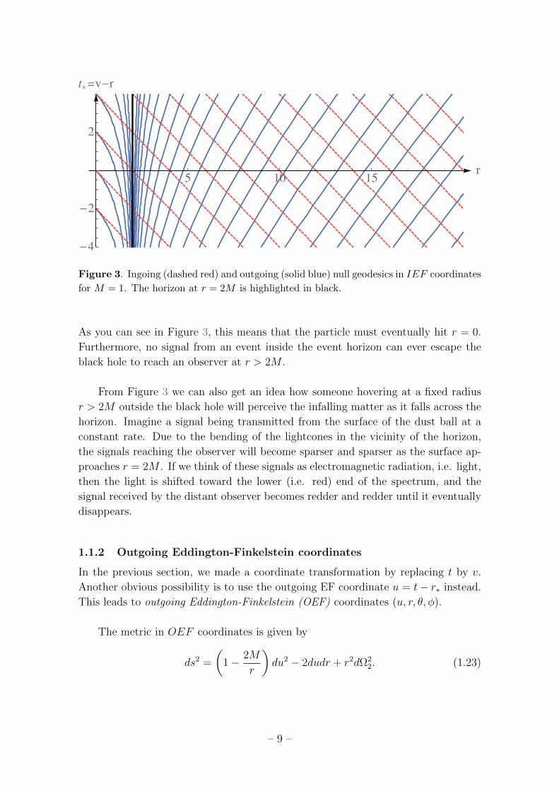
Figure 3. Ingoing (dashed red) and outgoing (solid blue) null geodesics in IEF coordinates
for M = 1. The horizon at r = 2M is highlighted in black.
As you can see in Figure 3, this means that the particle must eventually hit r = 0.
Furthermore, no signal from an event inside the event horizon can ever escape the
black hole to reach an observer at r > 2M .
From Figure 3 we can also get an idea how someone hovering at a fixed radius
r > 2M outside the black hole will perceive the infalling matter as it falls across the
horizon. Imagine a signal being transmitted from the surface of the dust ball at a
constant rate. Due to the bending of the lightcones in the vicinity of the horizon,
the signals reaching the observer will become sparser and sparser as the surface ap-
proaches r = 2M . If we think of these signals as electromagnetic radiation, i.e. light,
then the light is shifted toward the lower (i.e. red) end of the spectrum, and the
signal received by the distant observer becomes redder and redder until it eventually
disappears.
1.1.2 Outgoing Eddington-Finkelstein coordinates
In the previous section, we made a coordinate transformation by replacing t by v.
Another obvious possibility is to use the outgoing EF coordinate u = t− r∗ instead.
This leads to outgoing Eddington-Finkelstein (OEF) coordinates (u, r, θ, φ).
The metric in OEF coordinates is given by
ds2 =
(1− 2M
r
)du2 − 2dudr + r2dΩ2
2. (1.23)
– 9 –
-
-
*=+
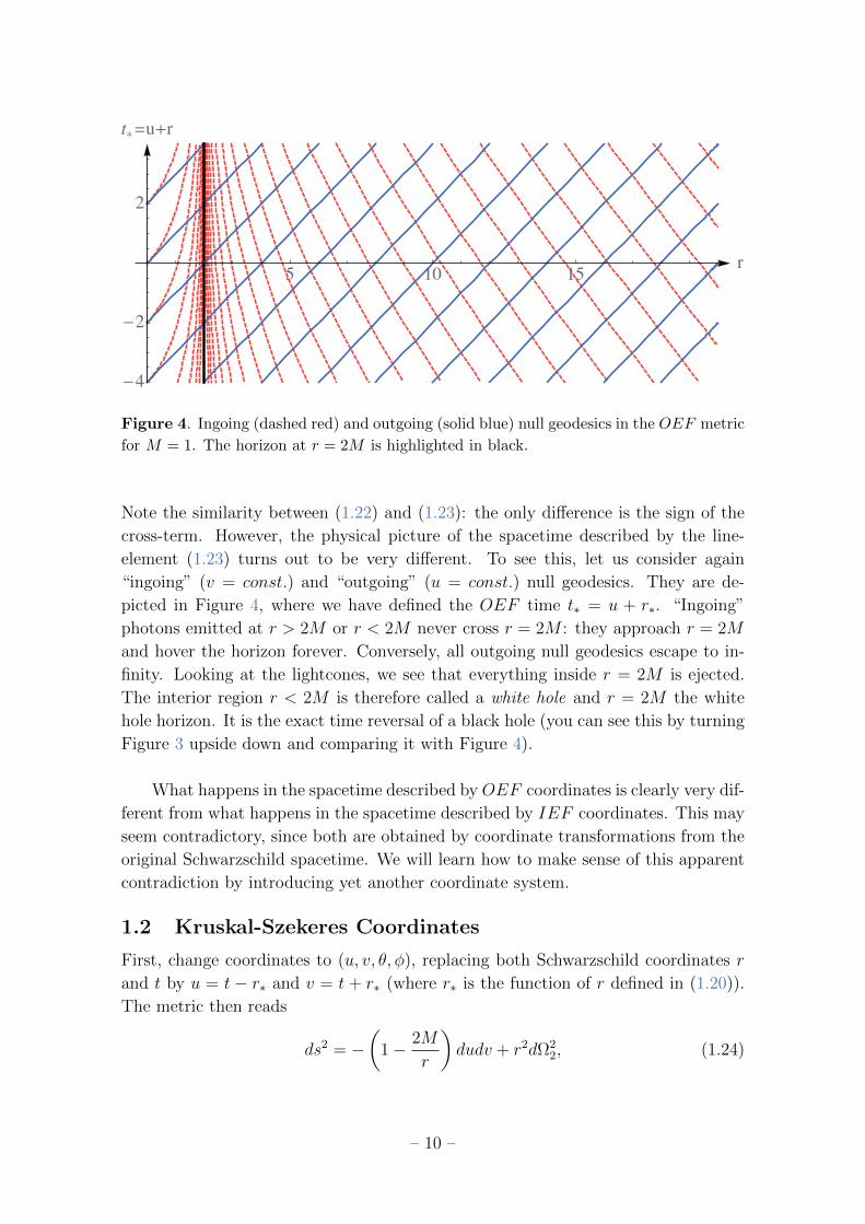
Figure 4. Ingoing (dashed red) and outgoing (solid blue) null geodesics in the OEF metric
for M = 1. The horizon at r = 2M is highlighted in black.
Note the similarity between (1.22) and (1.23): the only difference is the sign of the
cross-term. However, the physical picture of the spacetime described by the line-
element (1.23) turns out to be very different. To see this, let us consider again
“ingoing” (v = const.) and “outgoing” (u = const.) null geodesics. They are de-
picted in Figure 4, where we have defined the OEF time t∗ = u + r∗. “Ingoing”
photons emitted at r > 2M or r < 2M never cross r = 2M : they approach r = 2M
and hover the horizon forever. Conversely, all outgoing null geodesics escape to in-
finity. Looking at the lightcones, we see that everything inside r = 2M is ejected.
The interior region r < 2M is therefore called a white hole and r = 2M the white
hole horizon. It is the exact time reversal of a black hole (you can see this by turning
Figure 3 upside down and comparing it with Figure 4).
What happens in the spacetime described by OEF coordinates is clearly very dif-
ferent from what happens in the spacetime described by IEF coordinates. This may
seem contradictory, since both are obtained by coordinate transformations from the
original Schwarzschild spacetime. We will learn how to make sense of this apparent
contradiction by introducing yet another coordinate system.
1.2 Kruskal-Szekeres Coordinates
First, change coordinates to (u, v, θ, φ), replacing both Schwarzschild coordinates r
and t by u = t− r∗ and v = t + r∗ (where r∗ is the function of r defined in (1.20)).
The metric then reads
ds2 = −(
1− 2M
r
)dudv + r2dΩ2
2, (1.24)
– 10 –

where r = r(u, v) can be given in terms of u and v via (1.20) and r∗ = (v − u)/2.
This metric has a coordinate singularity at r = 2M , so it is only defined for r 6= 2M .
To remove the singularity, we define a new pair of coordinates U and V in the region
r > 2M by
U = − exp(− u
4M
)and V = exp
( v
4M
). (1.25)
Note that U < 0 and V > 0 for all values of r. The coordinates (U, V, θ, φ) are called
Kruskal-Szekeres (KS) coordinates. The Schwarzschild metric in KS coordinates is
(exercise):
ds2 = −32M3
rexp
(− r
2M
)dUdV + r2dΩ2
2, (1.26)
where r = r(U, V ) is defined in terms of U and V by the implicit equation
UV = −(r−2M
2M
)exp
(r
2M
).2
This metric is well-defined for r = 2M and indeed for all r > 0. Notice that
for r < 2M , we have UV > 0, which is incompatible with (1.25). Let us there-
fore forget the initial definitions of U and V in terms of the Schwarzschild coordi-
nates for now (much like we did for u and v when we went from Schwarzschild to
Eddington-Finkelstein coordinates), and instead investigate the new spacetime with
metric (1.26) an extended coordinate ranges −∞ < U, V <∞.
Figure 5 is a picture of the spacetime described by the KS metric. Since null lines
are conventionally plotted at 45, we define time and space coordinates T = U + V
and X = T − V , which label the vertical and horizontal axes in the figure. The
U and V axes are then at 45 to the T and X axes. At the horizon r = 2M , we
have UV = 0, which means either U = 0 or V = 0. This corresponds to the solid
diagonals. The singularity r = 0 corresponds to the (two branches of the) hyper-
bola described by UV = 1, which is represented by a wavy line (singularities will
always be represented by wavy lines). In general, surfaces of r = const. correspond
to hyperbolae UV = const. with UV < 1, as shown in blue on the diagram. Spatial
sections with t = const. have U/V = const. and |U/V | < 1, which corresponds to
straight lines through the origin with gradient between −1 and 1. Finally, ingoing
and outgoing null geodesics are respectively given by U = const. and V = const.
We can now see the relation between the different coordinate systems. The
original Schwarzschild coordinates (t, r, θ, φ) only cover region I. When we changed
to IEF and OEF coordinates, we extended our spacetime to regions II and III,
respectively. There is a new region that we only see in KS coordinates, region IV .
2We can write r explicitly as r(U, V ) = 2M [1 +W (−UV/e)] where e is Euler’s constant and W
stands for the Lambert W -function.
– 11 –
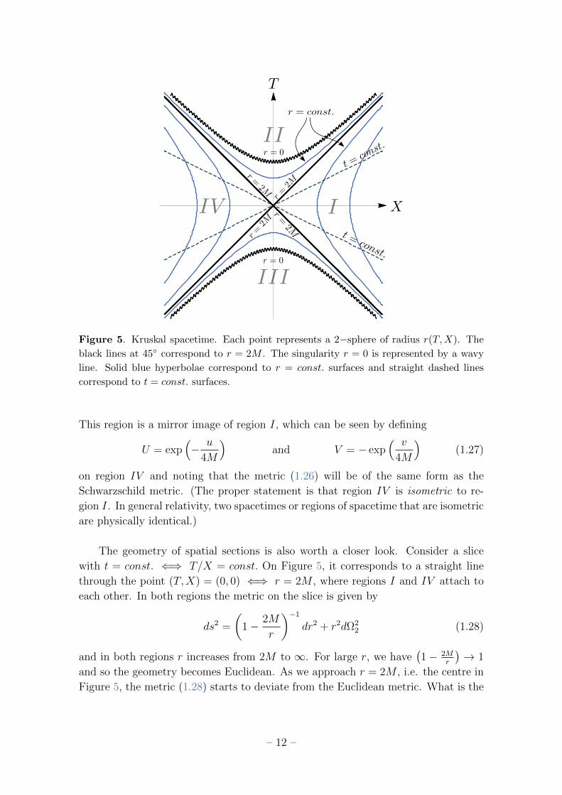
Figure 5. Kruskal spacetime. Each point represents a 2−sphere of radius r(T,X). The
black lines at 45 correspond to r = 2M . The singularity r = 0 is represented by a wavy
line. Solid blue hyperbolae correspond to r = const. surfaces and straight dashed lines
correspond to t = const. surfaces.
This region is a mirror image of region I, which can be seen by defining
U = exp(− u
4M
)and V = − exp
( v
4M
)(1.27)
on region IV and noting that the metric (1.26) will be of the same form as the
Schwarzschild metric. (The proper statement is that region IV is isometric to re-
gion I. In general relativity, two spacetimes or regions of spacetime that are isometric
are physically identical.)
The geometry of spatial sections is also worth a closer look. Consider a slice
with t = const. ⇐⇒ T/X = const. On Figure 5, it corresponds to a straight line
through the point (T,X) = (0, 0) ⇐⇒ r = 2M , where regions I and IV attach to
each other. In both regions the metric on the slice is given by
ds2 =
(1− 2M
r
)−1
dr2 + r2dΩ22 (1.28)
and in both regions r increases from 2M to ∞. For large r, we have(1− 2M
r
)→ 1
and so the geometry becomes Euclidean. As we approach r = 2M , i.e. the centre in
Figure 5, the metric (1.28) starts to deviate from the Euclidean metric. What is the
– 12 –

Figure 6. The Einstein-Rosen bridge with one spatial dimension suppressed. Each circle
represents a two-sphere in the three-dimensional analogue.
geometry near r = 2M? Since we cannot draw a three-dimensional surface, let us
suppress one angular coordinate by setting θ to its equatorial value θ = π2. Then the
metric is ds2 =(1− 2M
r
)−1dr2 + r2dφ2. It is not hard to show (exercise) that this
is just the metric on a so-called quartic surface x2 + y2 = (z2/8M + 2M)2 embed-
ded in three-dimensional Euclidean space E3 with cartesian coordinates x, y, z.3 The
geometry is shown in Figure 6, where two identical copies of the surface have been
attached to each other at the circle r = 2M . One side corresponds to region I and
the other side to region IV . This is known as the Einstein-Rosen bridge, which is
one example of a wormhole. Note that no observer can ever cross the wormhole, as
you can see clearly in the Kruskal diagram (and, further along in the lectures, in the
Penrose diagram for Kruskal space): in order to cross the wormhole from region I to
IV or vice-versa, the trajectory of the observer would have to be spacelike somewhere.
We can also get an intuitive sense for the strange sign change that appears in
the original Schwarzschild metric (1.1) between r > 2M and r < 2M , which makes r
appear like a time coordinate when r < 2M . Indeed, if r = 0 were just a “position in
space”, as one might naively think of it, it would seem that one could simply avoid
it by navigating around it. In Figure 5, we see that for anyone who has fallen across
the horizon, the singularity r = 0 is not a position in space — it becomes a moment
of time, as unavoidable as 9am tomorrow morning.
3Hint: Recall that the metric on E3 is ds2 = dx2 +dy2 +dz2. Consider the surface parametrised
by x = r cosφ, y = r sinφ and z =√
8M(r − 2M), show that it satisfies the quartic equation above
and find the metric induced on it. For an illustration see http://wolfr.am/WIRjK3.
– 13 –

Finally, we can justify in retrospect some of the coordinate extensions (analytic
continuations) that we performed rather ad-hoc in the last sections. For example,
consider the extension from region I covered by Schwarzschild coordinates to regions
I + II covered by IEF coordinates. The original coordinate system with time co-
ordinate −∞ < t < ∞ covers region I only. If we think of region I as a physical
spacetime in its own right, then a particle will hit a “boundary” (r = 2M) in fi-
nite proper time τ2M . In light of this, it seems physically quite reasonable to work
instead with the spacetime I + II obtained by extending the original coordinate
system, where this artificial boundary disappears.
1.3 Penrose Diagrams
In this section we introduce a useful way of representing the causal structure of an
infinite spacetime on a finite piece of paper. This involves performing a conformal
transformation on the metric:
Definition. A conformal transformation is a map from a spacetime (M, g) to a
spacetime (M, g) such that
gµν(x) = Λ(x)2gµν(x)
where Λ(x) is a smooth function of the spacetime coordinates and Λ(x) 6= 0 ∀ x.
Conformal transformations preserve the causal structure of a spacetime. To see
this, consider a vector V µ on M . Then it follows from Λ(x)2 > 0 that
gµνVµV ν > 0 ⇐⇒ gµνV
µV ν > 0
gµνVµV ν = 0 ⇐⇒ gµνV
µV ν = 0
gµνVµV ν < 0 ⇐⇒ gµνV
µV ν < 0.
(1.29)
Hence, curves that are timelike/null/spacelike with respect to g are timelike/null/
spacelike with respect to g. Furthermore, by consequence of the second line, null
geodesics for g correspond to null geodesics for g (whereas timelike/spacelike geodesics
for g are not necessarily geodesics for g).
The idea of a Penrose diagram is this. First, we use a coordinate transformation
on the spacetime (M, g) to bring “infinity” to a finite coordinate distance, so that
we can draw the entire spacetime on a sheet of paper. The metric will typically
diverge as we approach the “points at infinity”, i.e. the edges of the finite diagram.
To remedy this, we perform a conformal transformation on g to obtain a new metric
g that is regular on the edges. Then (M, g) is a good representation of the original
– 14 –
spacetime (M, g) insofar that it has exactly the same causal structure. It is custom-
ary to add the points at infinity to M to form a new manifold M . The resulting
spacetime (M, g) is what is called the conformal compactification of (M, g).
Note that the curvature tensors are in general not preserved under conformal
transformations, e.g. Rµνρσ 6= Rµ
νρσ, R 6= R etc. In that sense, the conformally com-
pactified spacetime (M, g) is unphysical: it provides a good representation of the
causal structure of the physical spacetime (M, g), but it should otherwise not be
viewed as a picture of what is going on (for example, as noted above, the geodesics
of massive test particles in (M, g) do not correspond to geodesics of massive test
particles in (M, g)).
1.3.1 Example 1: Minkowski space in 1 + 1 dimensions
The two-dimensional Minkowski metric is given by
ds2 = −dt2 + dx2 (1.30)
where −∞ < t, x <∞. We introduce light-cone coordinates u = t−x and v = t+x,
in which the metric gµν takes the simple form
ds2 = −dudv. (1.31)
Now, to shrink “infinity” down to a finite coordinate distance, we define a new set
of coordinates viau = tan u
v = tan v.(1.32)
These coordinates indeed have a finite range −π2< u, v < π
2(the range is open since
points with u, v = tan(±π2) = ±∞ are not points in spacetime). The line-element in
terms of u and v is
ds2 = − 1
(cos u cos v)2dudv. (1.33)
It diverges as u, v → ±∞ ⇐⇒ u, v → ±π2. Define a new metric gµν through a
conformal transformation on gµν :
ds2 = (cos u cos v)2 ds2 = −dudv. (1.34)
This metric is regular at the points at infinity where either u or v are equal to ±π2
and we can now add those points to the spacetime. The resulting spacetime (M, g)
is the conformal compactification of (M, g). Both spacetimes are shown in (u, v)
coordinates in Figure 7.
– 15 –

Figure 7. Left: Minkowski space (M, g) in (u, v) coordinates. The boundaries u, v = ±π2
are not part ofM and g diverges there. Some timelike and spacelike geodesics of g have been
included: lines with r = const. are represented by dashed curves and lines with t = const.
are represented by solid curves. Right: The Penrose diagram of conformally compactified
Minkowski space (M, g), with future/past timelike infinity i±, future/past null infinity J ±
and spacelike infinity i0. The timelike and spacelike geodesics of Minkowski space are
clearly not all geodesics for (M, g), since g is flat in (u, v) coordinates.
The two points (u, v) = (π2, π
2) and (−π
2,−π
2) are denoted by i±. All future (past)
directed timelike curves end up at i+ (i−), so we refer to i+ (i−) as future (past) time-
like infinity. Future directed null geodesics either end up at v = π2
with constant
|u| < π2
or at u = π2
with constant |v| < π2. This set of points is denoted by J +
(“scri-plus”) and referred to as future null infinity. An analogous definition holds
for past null infinity J − (“scri-minus”). Finally, spacelike infinity i0 denotes the set
of endpoints of spacelike geodesics, which corresponds here to (u, v) = (π2,−π
2) and
(u, v) = (−π2, π
2).
1.3.2 Example 2: Minkowski space in 3 + 1 dimensions
The four-dimensional Minkowski metric
ds2 = −dt2 + dx2 + dy2 + dz2 (1.35)
can be written in terms of spherical polar coordinates (t, r, θ, φ) by choosing an
arbitrary point as the origin, say x = y = z = 0. We then have
ds2 = −dt2 + dr2 + r2dΩ22 (1.36)
where dΩ22 is the round metric on the 2-sphere. Define light-cone coordinates u = t−r
and v = t+ r and perform the same transformation (1.32) as above to bring infinity
– 16 –

Figure 8. Left: The Penrose diagram of 3 + 1 dimensional Minkowski space with some
lines of constant r and t. Each point represents a 2−sphere. As the null geodesic shown
passes through r = 0, it emerges on another copy of the Penrose diagram whose points
represent the antipodes on the two-spheres. Right: The conformal compactification drawn
as a portion of the Einstein static universe with the same null geodesic.
to finite coordinate distance. The only difference to the previous analysis is that
since r ≥ 0, we have the additional constraint u ≤ v ⇐⇒ u ≤ v. The metric in
(u, v, φ, θ) coordinates reads
ds2 = − 1
(2 cos u cos v)2
[−4dudv + sin2 (v − u) dΩ2
2
](1.37)
and its conformal compactification corresponds to the spacetime (M, g) with metric
ds2 = (cos u cos v)2 ds2 = −4dudv + sin2 (v − u) dΩ22. (1.38)
and extended coordinate ranges −π/2 ≤ u, v ≤ π/2. On the Penrose diagram of
1 + 1 dimensional Minkowski space in Figure 7, u ≤ v implies that we only include
the part that lies to the right of the vertical line x = 0. The resulting diagram for the
3+1 space is shown in Figure 8. Every point on the diagram represents a two-sphere
of radius sin(v − u).
There exists a somewhat more illustrative way to picture the conformal com-
pactification. Define T = v + u and χ = v − u. The coordinate ranges are then
(exercise) −π < T < π and 0 < χ < π and the metric reads
ds2 = −dT 2 + dχ2 + sin2 χdΩ22. (1.39)
– 17 –

Figure 9. Eternally accelerating observers in Minkowski space. Their worldlines are shown
in blue and labelled by ξ. Events in the shaded region such as the black dot are hidden
to them. The Rindler horizon is the boundary between the shaded and unshaded regions.
Rindler space corresponds to the right wedge outlined by the dashed black null lines. The
straight dotted lines are lines of constant Rindler time η.
The spatial part dχ2 + sin2 χdΩ22 of this metric is just the round metric of a three-
sphere S3 parametrised by polar coordinates (χ, θ, φ). The spacetime (1.39) therefore
represents a static universe with spherical spatial slices, which corresponds to a fi-
nite portion of the Einstein static universe (ESU) whose topology is R×S3. This is
shown in Figure 8, and the Penrose diagram corresponds to that part of the region
wrapped around the cylinder facing out of the page.
1.3.3 Example 3: Rindler space in 1 + 1 dimensions
Rindler space is a subregion of Minkowski space associated with observers eternally
accelerated at a constant rate. The worldlines of these “Rindler observers” (acceler-
ating in the positive x-direction) is given by the hyperbolae xµxµ = −t2 + x2 = ξ2.
You can check (exercise) that the 4-acceleration aµ = d2xµ/dτ 2 along this worldline
is indeed constant: aµaµ = 1/ξ2.
Consider the one-parameter family of Rindler observers depicted in Figure 9.
The region x ≤ t is forever hidden to them, which makes the line x = t a horizon to
these observers.4Rindler space corresponds to the right wedge x > |t| foliated by the
4This horizon is different from the event horizon in the Schwarzschild black hole spacetime, since
the Schwarzschild horizon is observer/frame-independent, while the horizon here is associated with
– 18 –

Figure 10. The Penrose diagram for 1 + 1 dimensional Rindler space, seen as a portion of
Minkowski space. Some accelerated worldlines (curves of constant ξ) have been drawn for
ξ = 29 ,
25 ,
23 , 1,
32 ,
52 ,
92 . Note that all of the worldlines represent observers accelerating in the
postitive x−direction, even though they appear to bend toward the right for ξ > 1. This
distortion is a side effect of the coordinate transformation (u, v)→ (u, v).
worldlines of the accelerated observers in Figure 9. To obtain the Rindler metric, we
introduce a new set of space and time coordinates ξ and η in the subregion x > |t|of Minkowski space. As space coordinate we use ξ, which labels the hyperbolic
worldlines x2 − t2 = ξ2. As time coordinate we use the proper time η = tanh−1(t/x)
measured by a Rindler observer, synchronised such that η = 0 when the observer
passes the x-axis. The relation to Cartesian coordinates is
x = ξ cosh η and t = ξ sinh η (1.40)
and the coordinate ranges are 0 < ξ <∞ and −∞ < η <∞. The Minkowski metric
in (η, ξ) coordinates is
ds2 = −ξ2dη2 + dξ2. (1.41)
The proper time measured by an accelerated observer — i.e. a stationary (ξ = const.)
observer in Rindler coordinates — is τ = ξη. Since Rindler space is a subregion of
Minkowski space, the Penrose diagram is just a piece of Figure 7, as shown in Fig-
ure 10.
1.3.4 Example 4: Kruskal space in 3 + 1 dimensions
Recall the Kruskal metric (1.26):
ds2 = −32M3
rexp
(− r
2M
)dUdV + r2dΩ2
2.
a family of special observers/frames.
– 19 –

Define a new set of null coordinates via U = tan U and V = tan V , such that
−π2< U, V < π
2. Then the line-element becomes
ds2 = (2 cos U cos V )−2
[−4
32M3
rexp
(− r
2M
)dUdV + r2 cos2 U cos2 V dΩ2
2
](1.42)
We perform the usual conformal transformation, which leaves us with
ds2 = (2 cos U cos V )2ds2
= −432M3
rexp
(− r
2M
)dUdV + r2 cos2 U cos2 V dΩ2
2,(1.43)
and we add the points at infinity. The curvature singularity UV = 1 now corresponds
to
tan U tan V = 1 ⇐⇒ sin U sin V = cos U cos V ⇐⇒ cos(U + V ) = 0 (1.44)
which implies U + V = ±π2, or T = ±π
4if we define T and X through U = T − X
and V = T + X in analogy to section 1.2. The Penrose diagram including the points
at infinity and the singularity is shown in Figure 11. Also shown is the curve corre-
sponding to the surface of a collapsing star. If we only keep the region exterior to
the surface, we obtain the Penrose diagram for the collapsing star on the right. The
interior of the star is excluded since the stress-energy tensor is non-zero there and
spacetime is not described by the Schwarzschild metric. Therefore, regions I and
III are the only regions of Kruskal spacetime relevant to the description of a black
hole formed through stellar collapse.
1.3.5 Example 5: de Sitter space in 3 + 1 dimensions
The de Sitter metric is a solution of the Einstein equations in the presence of a
positive cosmological constant Λ > 0:
Rµν −1
2Rgµν + Λgµν = 0. (1.45)
It corresponds to a universe with uniform positive energy density and negative pres-
sure. To see this, note that (1.45) can be interpreted as the Einstein equations in
the presence of an energy momentum tensor
Rµν −1
2Rgµν = Tµν (1.46)
with Tµν = −Λgµν , which implies positive energy density T00 = Λ and negative uni-
form pressure Tii = −Λ for i = 1, 2, 3.
– 20 –

Figure 11. Left: The Penrose diagram for Kruskal space. The possible trajectory of the
surface of a collapsing star is shown — the region to the left of the curve corresponds to
the interior of the star, where spacetime is not described by the Kruskal metric. Right:
The Penrose diagram for a collapsing star. The curved line represents the surface and
the shaded region corresponds to the interior of the star. The horizon corresponds to the
dashed line.
de Sitter space admits a number of different coordinate systems, some of which
cover the whole space and some of which cover only part of it. The geometry of spatial
sections in these coordinates can also vary (closed, open, flat). One convenient set of
coordinates are closed global coordinates (t, χ, θ, φ) in which the line-element reads
ds2 = −dt2 + a2 cosh2(t/a)dΩ23, (1.47)
corresponding to a spacetime whose spatial sections are three-spheres with a time-
dependent radius a cosh(t/a).
The best way to picture de Sitter space is as a hyperboloid embdedded in
Minkowski space of one dimension higher (so 3 + 1 dimensional de Sitter space
is a hyperboloid in 4 + 1 dimensional Minkowski space). Since our illustrations
are restricted to three dimensions, let us suppress two of the angular coordinates
by setting χ = θ = π2. In that case, spatial cross sections are circles instead of
three-spheres and dΩ23 → dφ2. To see that this two-dimensional de Sitter space is
a hyperboloid embedded in three-dimensional Minkowski space, consider the surface
parametrised by T = a sinh(t/a), X = a cosh(t/a) cosφ and Y = a cosh(t/a) sinφ,
where T,X, Y are Cartesian coordinates in Minkowski space. Then it is easy to check
that the embedding 2 + 1 dimensional Minkowski metric ds2 = −dT 2 + dX2 + dY 2
reproduces (1.47) and furthermore that de Sitter space satisfies the equation of a
hyperboloid: −T 2 +X2 + Y 2 = a2. This is shown in Figure 12.
– 21 –
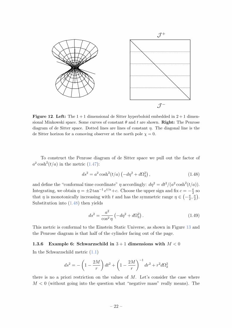
Figure 12. Left: The 1 + 1 dimensional de Sitter hyperboloid embedded in 2 + 1 dimen-
sional Minkowski space. Some curves of constant θ and t are shown. Right: The Penrose
diagram of de Sitter space. Dotted lines are lines of constant η. The diagonal line is the
de Sitter horizon for a comoving observer at the north pole χ = 0.
To construct the Penrose diagram of de Sitter space we pull out the factor of
a2 cosh2(t/a) in the metric (1.47):
ds2 = a2 cosh2(t/a)(−dη2 + dΩ2
3
), (1.48)
and define the “conformal time coordinate” η accordingly: dη2 = dt2/(a2 cosh2(t/a)).
Integrating, we obtain η = ±2 tan−1 et/a+c. Choose the upper sign and fix c = −π2
so
that η is monotonically increasing with t and has the symmetric range η ∈(−π
2, π
2
).
Substitution into (1.48) then yields
ds2 =a2
cos2 η
(−dη2 + dΩ2
3
). (1.49)
This metric is conformal to the Einstein Static Universe, as shown in Figure 13 and
the Penrose diagram is that half of the cylinder facing out of the page.
1.3.6 Example 6: Schwarzschild in 3 + 1 dimensions with M < 0
In the Schwarzschild metric (1.1)
ds2 = −(
1− 2M
r
)dt2 +
(1− 2M
r
)−1
dr2 + r2dΩ22
there is no a priori restriction on the values of M . Let’s consider the case where
M < 0 (without going into the question what “negative mass” really means). The
– 22 –

Figure 13. Left: The conformal compactifiction of de Sitter space viewed as a finite slab
of the Einstein static universe. Right: The Penrose diagram for the negative mass black
hole. The singularity at r = 0 can be seen from J +.
term(1− 2M
r
)= (1 + 2|M |
r) is then always positive and there are no singularities in
the metric except the curvature singularity at r = 0.
We can construct the Penrose diagram in the same manner as in the positive
mass case, by writing the metric in terms of u = t − r∗ and v = t + r∗ coordinates
(with the restriction r ≥ 0 ⇐⇒ v ≥ u) and proceeding with the conformal com-
pactification as usual. The Penrose diagram is shown in Figure 13.
Notice that this singularity is different from the black hole singularity: it can
be seen from J +. Conversely, the singularity inside the black hole is hidden behind
the horizon r = 2M . A singularity that can be seen from J + is known as a naked
singularity. The white hole has a naked singularity too, as it can be seen in Figure 11.
While naked singularities occur quite frequently in solutions to Einsteins equations,
their physical status is debated. Roger Penrose has formulated the cosmic censorship
hypothesis: “Nature abhors a naked singularity”, which encapsulates the expectation
that naked singularities (except for the Big Bang) are unphysical and do not occur
in the real world.
2 Charged & Rotating Black Holes
The Schwarzschild black hole is only the simplest among a number of black hole
solutions to the Einstein equations. In fact, the astrophysical black holes for which
– 23 –

we have observational evidence all appear to be rotating, while the Schwarzschild
solution has zero angular momentum. In this section we review two further, more
general, black hole solutions.
2.1 The Reissner-Nordstrom Solution
Gravity coupled to the electromagnetic field is described by the Einstein-Maxwell
action
S =1
16πG
∫ √−g (R− FµνF µν) d4x (2.1)
where Fµν = ∇µAν − ∇νAµ and Aµ is the electromagnetic (four-)potential. The
normalisation of the Maxwell term in (2.1) is such that the Coulomb force between
two charges Q1 and Q2 separated by a (large enough) distance r is G|Q1Q2|/r2. This
corresponds to geometrised units of charge.
The equations of motion derived from the variation of the Einstein-Maxwell
action are
Rµν −1
2Rgµν = 2
(FµλF
λν −
1
4gµνFρσF
ρσ
)∇µF
µν = 0.
(2.2)
They admit the spherically symmetric solution
ds2 = −(
1− 2M
r+Q2
r2
)dt2 +
(1− 2M
r+Q2
r2
)−1
dr2 + r2dΩ22, (2.3)
which is known as the Reissner-Nordstrom solution. The electric potential is A0 = Qr
and the other components of Aµ vanish. We therefore interpret Q as the charge of
the black hole (by analogy with the electric potential of a point charge) and M as its
mass. Without loss of generality we will assume that Q > 0. By a theorem analo-
gous to Birkhoff’s theorem, the Reissner-Nordstrom solution is the unique spherically
symmetric solution to the Einstein-Maxwell equations.
It is convenient to introduce the function
∆ = Q2 − 2Mr + r2 = (r − r+)(r − r−) (2.4)
where r± = M ±√M2 −Q2. The metric then reads
ds2 = −∆
r2dt2 +
r2
∆dr2 + r2dΩ2
2. (2.5)
There are three separate cases to look at: Q > M , Q < M and Q = M . Let’s
consider them in turn.
– 24 –

2.1.1 Super-Extremal RN: Q > M
If Q > M then ∆ has no real roots and the metric is regular for all r > 0. There is
a curvature singularity at r = 0. This is the same situation as for the negative mass
black hole, and the Penrose diagram looks exactly the same (Figure 13).
Note that an electron has charge e = 1.6×10⁻¹⁹ C and mass me = 9.1×10⁻³¹ kg.
In geometrised units this means Q = e/√
4πε0G = 1.4× 10⁻²⁹ kg, so QM . Could
it be that an electron is just a charged black hole? No. The electron is a quantum
mechanical object, whose Compton wavelength λ = h/mc = 2.4 × 10⁻¹² m is much
larger than its Schwarzschild radius rs = 2Gme/c2 = 1.4× 10−57m.
2.1.2 Sub-Extremal RN: Q < M
Now ∆ has two real roots r+ > r− and there are two coordinate singularities. As
always, we can remove them if we find a suitable coordinate system. Recalling our
strategy with the Schwarzschild metric, let us define a tortoise coordinate r∗via
∆
r2dr2∗ =
r2
∆dr2, (2.6)
in terms of which the metric takes the form
ds2 = −∆
r2(dt2 − dr2
∗) + r2dΩ22. (2.7)
Radial null geodesics are then given by the simple equation t ± r∗ = const. (and
θ = φ = const.). A solution of (2.6) with a convenient choice of sign and integration
constant is
r∗ = r +1
2κ+
ln
(r − r+
r
)+
1
2κ−ln
(r − r−r
), (2.8)
where
κ+ =r+ − r−
2r2+
> 0 and κ− =r− − r+
2r2−
< 0. (2.9)
Define the null coordinates u = t − r∗ and v = t + r∗ and ingoing Eddington-
Finkelstein coordinates (v, r, θ, φ). In terms of the latter, the metric becomes
ds2 = −∆
r2dr2 + drdv + r2dΩ2
2, (2.10)
which is regular for all r > 0, including r = r+ and r = r−. To understand the
spacetime structure close to r = r± we can use two different sets of Kruskal-type
coordinates at each of the two radii:
U± = − exp (−κ±u) and V ± = exp (κ±u) . (2.11)
This gives rise to the Penrose diagram shown in Figure 14. Notice that a timelike
trajectory can avoid r = 0, since the r = 0 singularity is timelike itself. In fact, to
hit r = 0, one must accelerate toward it (this time it is like a position in space).
– 25 –

Figure 14. The Penrose diagram for the sub-extremal Reissner-Nordstrom solution.
2.1.3 Extremal RN: Q = M
The metric of the extremal Reissner-Nordstrom solution is
ds2 = −(
1− M
r
)2
dt2 +
(1− M
r
)−2
dr2 + r2dΩ22, (2.12)
which has one coordinate singularity at r = r+ = r− = M . To get rid of it, define
the tortoise coordinate dr∗ = (1− Mr
)−2dr such that
ds2 = −(
1− M
r
)2
(dt2 − dr2∗) + r2dΩ2
2, (2.13)
and change to ingoing Eddington-Finkelstein coordinates (v, r, θ, φ), where v = t+r∗labels ingoing null geodesics, which should be clear from a look at (2.13). This leaves
us with the improved line-element
ds2 = −(
1− M
r
)dv2 + 2dvdr + r2dΩ2
2 (2.14)
which is regular at r = M . The inner and outer horizons have now coalesced. The
result is the Penrose diagram shown in figure (to come).
– 26 –

2.2 Rotating Black Holes
So far we have only discussed solutions with spherical symmetry. We now introduce
the Kerr-Newman solution (1965) to the Einstein-Maxwell equations, which describes
a rotating charged black hole of mass M , charge Q and angular momentum J ≡Ma
(so a is the angular momentum per unit mass). In Boyer-Lindquist coordinates
(t, r, θ, φ), in which the black hole rotates about the polar axis, the metric part of
the solution is given by
ds2 =−(
∆− a2 sin2 θ
Σ
)dt2 +
Σ
∆dr2 − 2
a sin2 θ
Σ
(r2 + a2 −∆
)dtdφ
+ Σdθ2 +
((r2 + a2)2 −∆a2 sin2 θ
Σ
)sin2 θdφ2
(2.15)
where where Σ = r2 + a2 cos2 θ and ∆ = r2 − 2Mr + Q2 + a2. The components of
the electromagnetic potential are
At =Qr
Σ, Aφ = −Qar sin θ
Σ, Ar = Aθ = 0. (2.16)
For a = Q = 0, we recover the Schwarzschild solution (1.1). For a = 0, we
recover the Reissner-Nordstrom solution (2.3). Finally, the solution is symmetric
under the simultaneous replacements φ → −φ and a → −a, so we can set a ≥ 0
without loss of generality.
When a black hole is rotating, there is no analogue of Birkhoff’s theorem. This
means that, during gravitational collapse with rotating matter, we cannot use the
same reasoning as in the spherically symmetric case to argue that, on the surface of
the collapsing matter, the metric should be of the form given above. All we can say
is that, after enough time has passed and matter and spacetime have “settled down”
to equilibrium, they will be described by the Kerr-Newman solution.
We will investigate the structure of the simple but illustrative special case of a
rotating black hole with zero charge Q = 0. The metric (2.15) then reduces to the
Kerr solution (1963):
ds2 = Σ
(dr2
∆+ dθ2
)+ (r2 + a2) sin2 θdφ2 +
2Mr
Σ
(a sin2 θdφ− dt
)2 − dt2 (2.17)
where ∆ = r2 − 2Mr + a2 and Σ = r2 + a2 cos2 θ. This metric is a solution to the
vacuum Einstein equations. It has coordinate singularities at
∆ = 0 ⇐⇒ r = r± = M ±√M2 − a2. (2.18)
– 27 –

Below we will show a coordinate transformation that removes them. It also has a
curvature singularity at
Σ = 0 ⇐⇒ r = 0 and cos θ = 0. (2.19)
The latter condition implies that the curvature singularity is only there when θ = π2,
i.e. when r = 0 is approached along the equator. When approached from any other
angle, there is no singularity at r = 0.
There are again three cases to consider: M < a, M = a and M > a. We will
concentrate on the M > a solution, for which there are two coordinate singularities at
r+ (the “outer” horizon) and r− < r+ (the “inner” horizon). To remove them, we do
a coordinate transformation to ingoing Kerr coordinates (v, r, θ, χ), where v = t+ r∗and r∗ and χ are defined by
dr∗ =r2 + a2
∆dr and dχ = dφ+
a
∆dr. (2.20)
The definition of χ implies that φ = const. does not correspond to χ = const. For
example, in order to stay at χ = const. as you fall in (dr < 0), you need to rotate
too: dφ = −a/∆dr. In terms of ingoing Kerr coordinates the metric becomes
ds2 =−(
∆− a2 sin2 θ
Σ
)dv2 + 2dvdr − 2
a sin2 θ
Σ(r2 + a2 −∆)dvdχ
− 2a sin2 θdχdr +
[(r2 + a2)
2 −∆a2 sin2 θ
Σ
]sin2 θdχ2 + Σdθ2.
(2.21)
There are no more factors of ∆ in the numerators and the metric is regular at r+
and r−. The only remaining singularity is the curvature singularity at Σ = 0.
To draw the Penrose diagram is more difficult because the metric is not spheri-
cally symmetric. Since the curvature singularity at r = 0 only appears when θ = π2,
the Penrose diagram should look very different for θ 6= π2
and θ = π2. In order to
represent both cases, it is customary to draw a Penrose diagram that is an amalgam
of the Penrose diagram for an observer falling in from the north pole (θ = 0) and of
that for an observer falling in in the equatorial plane (θ = π2) at fixed χ. Notice that
χ = const. means that φ is not constant, so the observer falling in at θ = π2
rotates
about the polar axis.
The procedure is very similar to that for the sub-extremal Reissner-Nordstrom
solution in section 2.1.2. First, perform a coordinate transformation to coordinates
(u, v, θ, φ) where u = t+ r∗ and v = t− r∗ with r∗ as defined in (2.20). Then, define
Kruskal-type coordinates U± and V ± close to r = r±, respectively, and draw the
– 28 –
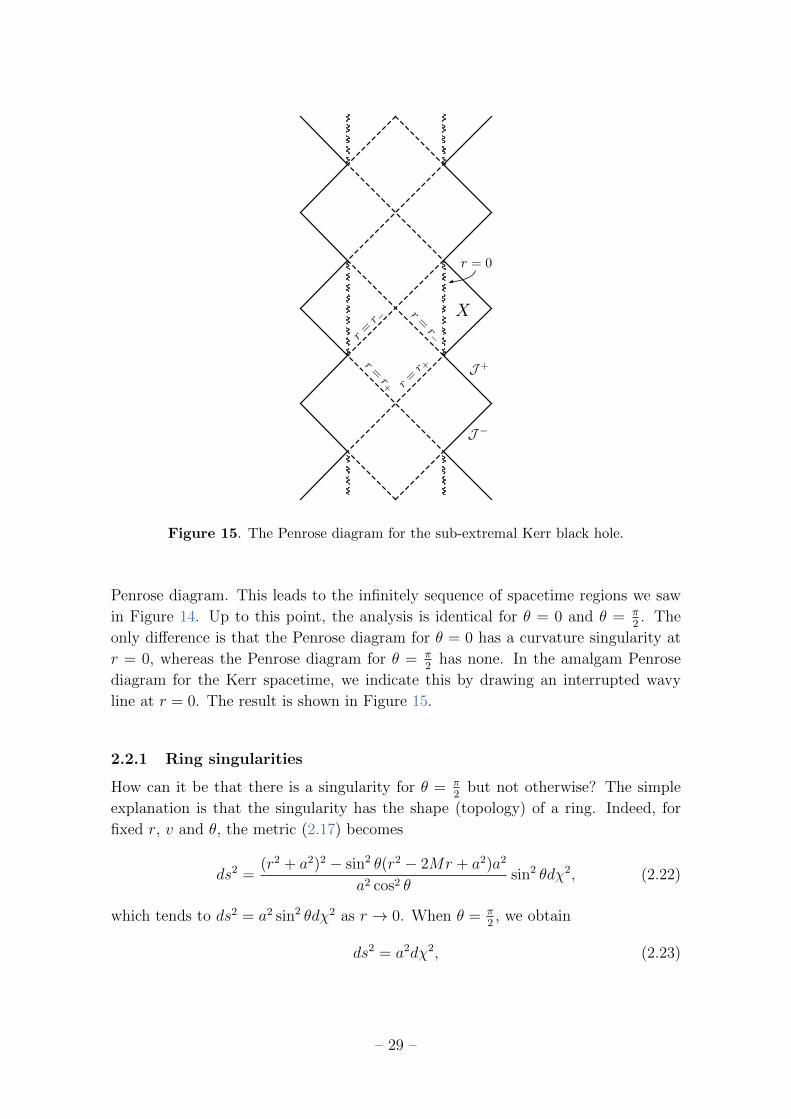
Figure 15. The Penrose diagram for the sub-extremal Kerr black hole.
Penrose diagram. This leads to the infinitely sequence of spacetime regions we saw
in Figure 14. Up to this point, the analysis is identical for θ = 0 and θ = π2. The
only difference is that the Penrose diagram for θ = 0 has a curvature singularity at
r = 0, whereas the Penrose diagram for θ = π2
has none. In the amalgam Penrose
diagram for the Kerr spacetime, we indicate this by drawing an interrupted wavy
line at r = 0. The result is shown in Figure 15.
2.2.1 Ring singularities
How can it be that there is a singularity for θ = π2
but not otherwise? The simple
explanation is that the singularity has the shape (topology) of a ring. Indeed, for
fixed r, v and θ, the metric (2.17) becomes
ds2 =(r2 + a2)2 − sin2 θ(r2 − 2Mr + a2)a2
a2 cos2 θsin2 θdχ2, (2.22)
which tends to ds2 = a2 sin2 θdχ2 as r → 0. When θ = π2, we obtain
ds2 = a2dχ2, (2.23)
– 29 –

the metric of a ring with radius a. If you travel toward r = 0 from any other angle
than θ = π2, you will not encounter the singularity. Instead, you will fall through the
interior of the “ring” and emerge in a new region of spacetime.
2.2.2 Closed Timelike Curves
A closed timelike curve (CTC), also called a time machine, is a curve that is every-
where timelike and that eventually returns to where it started from in spacetime.
CTCs have been extensively explored in the context of general relativity. In fact,
they are ubiquitous and appear in a number of spacetimes that are solutions to the
Einstein equations.
Kerr spacetime is one such example: region X in Figure 15 contains CTCs. To
see this, consider a curve in region X at fixed t, θ = π2
and r < 0. Then
ds2 =
(r2 + a2 +
2Ma
r
)dχ2. (2.24)
Close enough to the singularity, where r is small and negative, r < 0 and
|r| < 2Ma/(r2 + a2), (2.24) is negative and the curve is timelike. Since χ is a
periodic coordinate with χ ≡ χ+ 2π, the curve is also closed: it is a CTC.
However, it turns out that region X is unphysical. Much like in the case of
the sub-extremal RN solution of section 2.1.2, the inner horizon at r = r− becomes
a curvature singularity in the presence of the smallest perturbations to the Kerr
metric: at the inner horizon, perturbations are infinitely blueshifted, which leads to
divergences in the curvature scalars.
3 Killing Vectors & Killing Horizons
So far we have produced a number of different black hole solutions and looked at
some of their features. In this section we introduce the concepts and machinery that
we will need to really understand the structure of black hole spacetimes.
Notation: to denote partial derivatives we use shorthand notations such as ∂t = ∂∂t
and ∂µ = ∂∂xµ
as well as X,µ = ∂µX when applied to a tensor X.
3.1 Symmetries & Killing Vectors
Let (M, g) be a Lorentzian manifold. Given a smooth vector field ξ on M , an integral
curve of ξ is a curve γ : R → M whose tangent vector is equal to ξ at every point
– 30 –

p ∈ γ. This can be expressed as the demand that
ξp(f) =d
dλ(f γ(λ))
∣∣∣∣p
(3.1)
for all smooth functions f : M → R. Equivalently, given a coordinate system xµ on
M , the components of ξ in that coordinate system must satisfy
ξµp =d
dλxµ(γ(λ))
∣∣∣∣p
, (3.2)
where λ parametrises γ.
When ξ is smooth and everywhere non-zero, the set of integral curves form a
congruence: every point p ∈M lies on a unique integral curve. Given any congruence
there is an associated one-parameter family of diffeomorphisms from M onto itself,
defined as follows: for each s ∈ R, define hs : M → M , where hs(p) is the point
parameter distance s from p along ξ, i.e. if p = γ(λ0) then hs(p) = γ(λ0 + s). These
transformations form an abelian group: the composition law is hs ht = hs+t, the
identity is h0 and the inverse is (hs)−1 = h−s.
This leads to the concept of the Lie derivative Lξ along the vector field ξ. When
applied to a vector V at point p it is defined as
(LξV )p = limδλ→0
Vp − (hδλ)∗Vh−δλ(p)
δλ. (3.3)
Here (hs)∗ denotes the push-forward associated with the group element hs, which
maps a vector defined at p to a vector defined at hs(p). It can be shown (exercise)
that the Lie derivative of a vector is equal to the bracket
(LξV )p = [ξ, V ]p
where [X, Y ]µ = XνY µ,ν − Y νXµ
,ν .
The Lie derivative can be applied to any tensor on M , with appropriate defini-
tions analogous to (3.3). In particular, given a metric tensor g on M , we can take
its Lie derivative. Since the components of g transform covariantly (whereas vector
fields transform contravariantly), the Lie derivative of g involves the pull-back h∗s,
which maps a covector at hs(p) to a covector at p:
(Lξg)p = limδλ→0
gp − (hδλ)∗ghδλ(p)
δλ. (3.4)
It can then be shown that
(Lξg)µν = ∇µξν +∇νξµ. (3.5)
– 31 –

If the metric does not change under the transformation hs we say that the transfor-
mation is an isometry and that the metric has a symmetry. In this case Lξg = 0,
which implies
∇µξν +∇νξµ = 0. (3.6)
This is known as Killing’s equation and a vector ξ that satisfies (3.6) is a Killing
vector. Note that this equation implicitly involves the metric, which is hidden in
∇. Finding the symmetries of a spacetime amounts to finding the vectors that sat-
isfy the Killing equation; this can be done either by inspection or by integrating (3.6).
A useful fact to know when looking for Killing vectors is the following. Given
any vector field ξ we can (locally) find a coordinate system (x1, x2, x3, x4) in which
ξ takes the form
ξ =∂
∂x1, (3.7)
i.e. ξµ = (1, 0, 0, 0). This implies that
(Lξg)µν =∂gµν∂x1
. (3.8)
Hence, if we find a coordinate system in which gµν is independent of one of the
coordinates, say y, then we know that ∂∂y
must be a Killing vector since
(L ∂∂yg)µν =
∂gµν∂y
= 0. (3.9)
The converse statement is not true: if gµν depends on all the coordinates, that does
not mean that that g has no Killing vectors.
3.1.1 Example 1: Schwarzschild
Using the fact above, a quick look at the Schwarzschild metric
ds2 = −(
1− 2M
r
)dt2 +
(1− 2M
r
)−1
dr2 + r2dΩ22
reveals the two Killing vectors k = ∂t and m = ∂φ. This means that Schwarzschild
spacetime is static and axisymmetric:
Definition. An asymptotically flat spacetime is stationary if it admits a Killing
vector k such that k2 → −1 asymptotically. If in addition the metric is invariant
under t↔ −t, the spacetime is static.
Definition. An asymptotically flat spacetime is axisymmetric if it admits a Killing
vector ` that is spacelike asymptotically and whose integral curves are closed.
– 32 –

Schwarzschild spacetime is not just axisymmetric but spherically symmetric: it
has two more spacelike Killing vectors, which together with ∂φ generate the symme-
tries of a sphere — the SO(3) transformations. The other two Killing vectors cannot
be “read off” from the metric but they can be found by solving Killing’s equation.
3.1.2 Example 2: Kerr-Newman
The Kerr-Newman solution (2.15)
ds2 =−(
∆− a2 sin2 θ
Σ
)dt2 +
Σ
∆dr2 − 2
a sin2 θ
Σ
(r2 + a2 −∆
)dtdφ
+ Σdθ2 +
((r2 + a2)2 −∆a2 sin2 θ
Σ
)sin2 θdφ2
is axisymmetric and stationary: since gµν is independent of t and φ, it has Killing
vectors k = ∂t and ` = ∂φ. However, the metric is not invariant under t ↔ −t due
to the dtdφ term, so it is not static.
A number of uniqueness theorems, proved between 1967 and 1975, have estab-
lished the remarkable fact that the two-parameter Kerr family (parameters M and
J) is the unique stationary asymptotically flat solution of the vacuum Einstein equa-
tions and that the three-parameter Kerr-Newman family (parameters M , J and Q)
is the unique stationary asymptotically flat black hole solution of the electrovacuum
Einstein-Maxwell equations.
3.2 Conservation Laws
In classical physics, the presence of symmetries is very closely tied to the existence
of conservation laws. As we shall see in this section, this is also the case in general
relativity. We first take a look at the geodesic motion of test particles.
Consider the action of a particle in a spacetime (M, g) moving on a curve γ with
parameter λ and endpoints A and B. Pick a coordinate system xµ and denote the
coordinates of the curve by xµ(λ). Then the action for γ is given by
I (xµ) = m
∫dτ = m
∫ λB
λA
√−gµν
dxµ
dλ
dxν
dλ. (3.10)
If we deform the curve by a small amount δxµ(λ) and require the action to be
stationary with respect to this variation, we obtain the Euler-Lagrange equations:
δI
δxµ= 0 =⇒ ∇(λ)x
µ ≡ d
dλxµ + Γµρσx
ρxσ ∝ xµ. (3.11)
– 33 –

The dot denotes differentiation with respect to λ. The solutions to (3.11) are the
geodesics in (M, g). If the right hand side vanishes, ∇(λ)xµ = 0, the geodesic is said
to be affinely parametrised and λ is an affine parameter. If we set λ = τ then (3.11)
reduces tod2xµ
dτ 2+ Γµρσ
dxρ
dτ
dxσ
dτ= 0. (3.12)
For the purpose of finding geodesics we can cast (3.10) into a more useful form by
introducing an independent function e(λ) (called the auxiliary field or einbein):
I (xµ, e) =1
2
∫ λB
λA
dλ[e−1(λ)gµν x
µxν −m2e(λ)]. (3.13)
To see that this is equivalent to (3.10), notice that from δI/δe = 0 we get
− e−2gµν xµxν −m2 = 0 =⇒ e =
1
m
√−gµν xµxν =
1
m
dτ
dλ(3.14)
and from δI/δxµ we get
d
dλxµ + Γµρσx
ρxσ = (e−1e)xµ. (3.15)
This equation is already the geodesic equation ∇(λ)xµ = (e−1e)xµ and (3.14) re-
lates e to the choice of parameter λ. To turn this into the equation for an affinely
parametrised geodesic, we need to set e = 0. Then dτ/dλ = const., which implies
that λ = aτ + b.
Consider now an infinitesimal translation of the curve γ along a Killing vector
field k (leaving e unchanged). In the coordinate chart xµ this corresponds to
xµ → xµ + αkµ (3.16)
where α is an infinitesimal constant. Then the action will be changed by an amount
δI = I(xµ + αkµ, e)− I(xµ, e)
=α
2
∫dλ[e−1(gµν k
µxν + gµν xµkν + gµν,σx
µxνkσ)]
=α
2
∫dλ[e−1 (gµν x
σxνkµ,σ + gµν xµxσkν,σ + gµν,σx
µxνkσ)]
=α
2
∫dλ[e−1xµxν (gσνk
σ,µ + gµσk
σ,ν + gµν,σk
σ)]
=α
2
∫dλ[e−1xµxν (∇µkν +∇νkµ)
]= 0
(3.17)
where the last line follows from the fact that k satisfies Killing’s equation. To get
from the second to the third line we used the fact that kµ = ddτkµ = dxν
dτ∂νk
µ = xνkµ,ν .
– 34 –

We see that k being Killing leads to a symmetry of the particle action. Associated
with this symmetry is a quantity (charge) that is conserved along geodesics:
Claim. Let k be a Killing vector. Then
Q = kµpµ (3.18)
is conserved along geodesics, where pµ is the momentum of the particle defined by
pµ =∂L∂xµ
= e−1gµν xν = mgµν
dxν
dτ. (3.19)
The last equality follows from equation (3.14) for e.
Proof. Consider a small variation δxµ = αkµ generated by the Killing vector k.
Set λ = τ for simplicity (the proof for general λ is similar). As shown above, such
variations leave the action invariant: δI = 0. Defining the Lagrangian density L as
I =∫Ldλ, we then have
∂L∂xµ
δxµ +∂L∂xµ
δxµ = 0. (3.20)
Using the Euler-Lagrange equations
∂L∂xµ
=d
dτ
∂L∂xµ
= pµ, (3.21)
the previous equation can be written as
0 = pµαkµ + pµαk
µ = αd
dτ(kµpµ) = α
d
dτQ. (3.22)
Therefore Q is constant along geodesics.
3.2.1 Example 1: Schwarzschild
Recall the Killing vector k = ∂t in Schwarzschild spacetime. Then kµ = (1, 0, 0, 0)
and we have
Q = kµpµ = kµmgµν xν = mg00x
0 = −m(
1− 2M
r
)dt
dτ≡ −E, (3.23)
where we have identified Q with minus the energy of the particle in the rest frame
of the black hole. This agrees with the the definition of the constant ε = E/m in
equation (1.9) of section 1.
The conserved quantity associated with ` = ∂φ is
Q = mg33x3 = mr2 sin2 θφ ≡ J, (3.24)
the angular momentum of the particle along the axis of symmetry as measured by
an observer at rest at infinity.
– 35 –

3.2.2 Example 2: Kerr
The vectors k and ` are also Killing vectors for the Kerr metric (2.15,2.17):
ds2 = Σ
(dr2
∆+ dθ2
)+ (r2 + a2) sin2 θdφ2 +
2Mr
Σ
(a sin2 θdφ− dt
)2 − dt2.
In Schwarzschild spacetime, you (or a test particle) can travel along integral curves of
k = ∂t anywhere outside the horizon — you will then appear stationary5 to observers
at infinity, since your position in space is not changing. This is possible because g00 is
negative everywhere for r > 2M , so that k2 = g00 is negative and the integral curves
of k are timelike. It turns out that this is not the case in Kerr spacetime: there
is a region around the outer horizon, called the ergosphere or ergoregion, in which
it is impossible for you (and any test particle) to remain stationary with respect to
observers at infinity — everything rotates. This happens because
g00 = −(
1− 2Mr
Σ
)(3.25)
becomes positive in the region
2Mr
Σ> 1 =⇒ ξ(r) ≡ Σ− 2Mr = r2 + a2 cos2 θ − 2Mr < 0, (3.26)
part of which lies outside the outer horizon r = r+ when a 6= 0. This is easy to
see by noting that the equation for ξ(r) is a parabola with roots at r± = M ±√M2 − a2 cos2 θ and r+ is bigger than r+ = M +
√M2 − a2 for θ 6= 0, π. Hence g00
is positive in the ellipsoidal region r+ < r < r+, which has a maximum extent on the
equator θ = π2
where r+ = M +√M2 + a2.
In the ergoregion, orbits of ∂t are not timelike, so you cannot travel along them
and remain stationary with respect to observers at infinity. In order for a curve
xµ = (t, r, θ, φ) to be timelike, its tangent vector uµ = dxµ/dτ must satisfy u2 = −1.
But in the ergoregion, every term in u2 = gµνuµuν is positive except for gtφu
tuφ,
which means that uφ = dφ/dτ must be non-zero. Moreover, since ut > 0 for a
future-directed worldline and gtφ < 0, uφ must be positive. Any timelike worldline is
therefore dragged around in the direction of rotation of the black hole. This effect is
an example of frame dragging.
3.2.3 Example 3: The Penrose Process
The Penrose process is a process that allows you to extract energy from a rotating
black hole. Imagine sending a particle into the ergoregion. Prepare it carefully such
5The word “stationary” here has nothing to do with the definition of a stationary spacetime.
When used to describe the relative motion of one observer or test particle with respect to another
observer, stationary just means “not moving in space” from the point of view of the latter.
– 36 –

that, once in the ergoregion, it decays into two particles, one of which falls into the
black hole and one of which escapes the ergoregion again. Denote the energy of the
initial particle by E = −kµpµ and that of the final particles by E1 = −kµpµ1 and
E2 = −kµpµ2 , where k is the asymptotically timelike Killing vector. Conservation of
four-momentum pµ = pµ1 + pµ2 implies that E = E1 +E2. The fact that k is spacelike
in the ergoregion allows you to arrange the decay such that the energy of the particle
that falls into the black hole is negative with respect to you: E1 = kµpµ1 < 0. To see
this, choose a coordinate system in which kµ = (0, x, 0, 0). Prepare your decay such
that pµ1 = (1, y, 0, 0), where y is small enough for p1 to be timelike and adjusted such
that xy > 0. Then E1 is negative and E2 > E: the particle that reemerges from the
ergoregion has more energy than the particle you sent in.
3.3 Hypersurfaces
Let S(x) be a smooth function of the spacetime coordinates. Consider the family of
hypersurfaces S(x) = const. The normal vector to S(x) = const. is given by
nµ = f(x)gµν∂νS, (3.27)
where f(x) is an arbitrary (smooth) normalisation function. A hypersurface is space-
like (timelike) when n is timelike (spacelike) everywhere on it. When the hypersurface
is timelike (spacelike) we can always find an f(x) such that n2 = −1 (n2 = +1). A
hypersurface is null when n is null, n2 = 0.
3.3.1 The induced metric
Consider a spacelike (timelike) hypersurface Σ in a spacetime (M, g). Normalise the
normal n to Σ such that n2 = −1 (n2 = +1). Then the induced metric h on Σ is
given by
hµν = gµν + nµnν . (3.28)
The metric h is the restriction of g onto Σ: while h is degenerate on the full tangent
space at any point p ∈ Σ, it is positive definite for spacelike Σ (Lorentzian for time-
like Σ) on the subspace of the tangent space spanned by vectors tangent to curves
in Σ (i.e. vectors v that satisfy v.n = 0).
To give an example, consider a spatial slice Σ defined by S(x) = t = const. in 3+1
dimensional Minkowski space with Cartesian coordinates (t,x). Then nµ = (1, 0, 0, 0)
and
hµν = gµν + nµnν = diag(−1, 1, 1, 1) + diag(1, 0, 0, 0) = diag(0, 1, 1, 1). (3.29)
On the spatial slice Σ, h is just the positive definite three-dimensional flat Euclidean
metric. Next, consider a timelike hypersurface Σ defined by S(x) = x1 = const. with
– 37 –

normal nµ = (0, 1, 0, 0). The induced metric on it is hµν = diag(−1, 0, 1, 1), which
carries Lorentzian signature on the subspace of the tangent space spanned by vectors
tangent to Σ.
3.3.2 Null hypersurfaces
For a null hypersurface Σ, the normal n to Σ is also tangent to Σ, since, by defini-
tion, a vector t is tangent to Σ if t.n = 0. This is satisfied by n itself when it is null:
n.n = 0. When the normal is null we will henceforth use the symbol ` instead. The
normal ` is tangent to curves xµ(λ) in Σ: `µ = dxµ
dλ. In fact, the integral curves of `
are null geodesics :
Claim: For a null hypersurface Σ, the integral curves in Σ of the normal ` are null
geodesics.
Proof: For `µ = fgµν∂νS we have
`.∇`ν = `µ∇µ(fgνρ∂ρS)
= `µ(∇µf)gνρ∂ρS + f`µgνρ∇µ∂ρS
= (`.∇f)f−1`ν + f`µgνρ∇µ∂ρS.
(3.30)
The second term reduces as follows:
`µfgνρ∇µ∂ρS = f`µgνρ∇ρ∂µS
= f`µgνρ∇ρ(f−1`µ)
= fgνρ(∇ρf−1)`2 + `µgνρ∇ρ`µ
=1
2gνρ∇ρ(`
2)
∝ `ν
(3.31)
using the fact that `2 = 0 on Σ in the third line. In the last line, note that `2 = 0
on Σ does not necessarily imply ∇ρ(`2) = 0, because `2 can be non-zero outside of
Σ and hence its derivative can be non-zero. However, any non-zero contribution to
∇ρ(`2) must be proportional to the normal to Σ: ∇ρ(`
2) ∝ `ρ. Together with (3.30)
this implies that `.∇`ν ∝ `ν and therefore the integral curves of `µ are geodesics.
If the integral curves of `µ are not affinely parametrised, then we can always
find some function h(x) such that ˜µ = h(x)`µ has affinely parametrised integral
curves, i.e. ˜.∇˜µ = 0. These curves are called the null geodesic generators of the
null hypersurface.
3.4 Killing Horizons
A null hypersurface Σ is a Killing horizon of a Killing vector ξ if ξ is normal to Σ
on Σ. Let ` be normal to Σ and affinely parametrised such that `.∇` = 0. Then, for
– 38 –

some function f , ξ = f` on Σ. It follows that ξ satisfies
ξµ∇µξν = f`µ∇µ(f`ν)
= f`µ`ν∇µf + f 2`µ∇µ`ν
= f`ν`µ∇µf
≡ κξν
(3.32)
on Σ. In the last line we have defined κ, the surface gravity : ξµ∇µξν = κξν . It takes
its name from the fact that κ is constant over the horizon and equals the force that
an observer at infinity would have to exert in order to keep a unit mass at the horizon.
3.4.1 Example 1: Schwarzschild
In Schwarzschild spacetime, the surfaces of constant r are the “cylinders”of con-
stant S(r) = r and the black hole horizon corresponds to the particular surface
S(r) = 2M . To find the normal vector `µ = fgµν∂νS to the horizon, let us work in
IEF coordinates. We need the inverse of the IEF metric (1.22), which is given by
gµν =
0 1 0 0
1(1− 2M
r
)0 0
0 0 1/r2 0
0 0 0 1/r2 sin2 θ
. (3.33)
The normal vector to the surface S(r) = 2M is then
`µ = f(gvr∂rS, grr∂rS, 0, 0) = f
(1,(1− 2M
r
), 0, 0
)= f(1, 0, 0, 0) = f∂v. (3.34)
This vector is null at r = 2M since `2 = f 2grr = f 2(1− 2M
r
)= 0 at r = 2M . Hence
r = 2M is a null hypersurface. ` = f∂v is a Killing vector (since gµν is independent
of v) and it is timelike everywhere outside the horizon.
Remember that we already encountered a timelike Killing vector in Schwarzschild
spacetime: ∂t in Schwarzschild coordinates. In fact ∂t and ∂v are the same vector field.
To check this, denote Schwarzschild coordinates by (t, r, θ, φ) and IEF coordinates
by (v, r, θ, φ). Then
dv = dt+(1− 2M
r
)−1dr
dr = dr
dθ = dθ
dφ = dφ
(3.35)
and therefore
∂t =∂v
∂t∂v +
∂r
∂t∂r +
∂θ
∂t∂θ +
∂φ
∂t∂φ = ∂v. (3.36)
– 39 –

The surface gravity κ is evaluated most easily in IEF coordinates. The equa-
tion (3.32) defining κ is a vector equation so we only need to evaluate one of its
components. For ξ = ∂v, the µ = v component of ξσ∇σξµ is
ξσ∇σξv = ξσξv,σ + ξσΓvσρξ
ρ = Γvvv. (3.37)
Now
Γvvv =1
2gvσ (gvσ,v + gσv,v − gvv,σ) =
1
2gvr(−gvv,r) =
M
r2, (3.38)
which, on the horizon, reduces to Γvvv = 1/4M . Substitution into (3.37) then gives
κ = 1/4M .
Note that the particular normalisation of ξ is important. Had we used a vec-
tor with a different normalisation ξ = cξ we would have obtained ξ.∇ξν = (cκ)ξν ,
leading to a different value κ = cκ for the surface gravity. In Schwarzschild space-
time, the normalisation that leads to κ = 1/4M is fixed by requiring that ξ2 = −1
asymptotically.
3.4.2 Example 2: Kerr
The Killing horizon of a Kerr black hole is slightly more complicated in an interesting
way. Recall the Killing vectors k = ∂t and m = ∂φ of the Kerr-Newman black hole in
Boyer-Lindquist coordinates (t, r, θ, φ) of section 3.1.2. Let’s consider the zero charge
case of the Kerr black hole. In Kerr coordinates (v, r, θ, χ) — defined above (2.20)
— the Killing vectors correspond to k = ∂v = ∂t and m = ∂χ = ∂φ. The frame
dragging effect translates to the fact that k is not normal to the horizon. Instead,
for the rotating Kerr black hole, the normal to the horizon is a combination of k and
m (exercise) :
ξ = k + ΩHm, (3.39)
where ΩH = a/(r2+ + a2) is interpreted as the angular velocity of the black hole.
The intuition here is that as you move forward in time along a null generator of the
horizon, you also have to rotate by a certain amount. Given ξ we can evaluate the
surface gravity κ+ on the outer horizon r = r+ using ξ.∇ξν = κξν , which evaluates
to (exercise)
κ+ =r+ − r−
2(r2+ + a2)
. (3.40)
3.5 Black Hole Uniqueness
As already mentioned in section 3.1.2, the Kerr-Newman three-parameter family
is the unique stationary black hole solution of the Einstein-Maxwell theory. An
– 40 –
equilibrium black hole in the presence of the electromagnetic field is therefore fully
characterised by the three numbers M , J and Q.
However, the electromagnetic field is only one among many matter fields in
Nature. Through a series of theorems known as “no hair” theorems it has been es-
tablished that, in general, black holes have no other properties besides mass, angular
momentum and charge (of whichever fields are present). To illustrate the general
spirit of these proofs, we look at a simple example here.
Claim: A static black hole cannot be the source of a real (minimally coupled) scalar
field.
Proof: Let φ be a real scalar field that satisfies the Klein-Gordon equation
∇2φ−m2φ = 0. (3.41)
By the word “static” in the claim we mean that scalar field and spacetime (i.e. the
metric field) have settled down to equilibrium, which implies that the scalar field
does not vary in time anymore: “φ = 0”. In covariant language the statement is that
there exists a timelike Killing vector k (= ∂t) of the metric such that kµ∇µφ = 0.
Given k we can foliate the spacetime by t = const. hypersurfaces whose unit normals
n are proportional to k, n ∝ k. The black hole horizon is a Killing horizon of k.
Consider the integral
I =
∫R
φ(∇2φ−m2φ)√−gd4x, (3.42)
where V ⊂M is the spacetime region outside of the horizon. From the Klein-Gordon
equation (3.41) it follows immediately that I = 0. On the other hand, using Stokes’
theorem to integrate by parts the first term, we get
I =
∫V
(−gµν∇µφ∇νφ−m2φ2)√−gd4x+
∫∂V
φ∇µφdSµ (3.43)
where ∂V is the boundary of the region V and dSµ is the normal surface element on
∂V .
We now show that the surface integral in (3.43) vanishes identically. There
are four contributions to ∂V : the horizon r = 2M , the surfaces t = ±∞ and the
surface r → ∞ (the “sphere at infinity”). On the horizon and on the t = ±∞surfaces, the normal surface element is proportional to k, so the integrand vanishes:
∇µφdSµ ∝ kµ∇µφ = 0. We are left with the boundary term at r →∞. To see that
– 41 –

this vanishes too, note that since the spacetime is static and asymptotically flat, the
metric takes the form
ds2 = f(r)dt2 + g(r)dr2 + r2dΩ22 (3.44)
where f(r) = −1 + f1r−1 + O(r−2) and g(r) = 1 + g1r
−1 + O(r−2). Using
∇2 = 1√−g∂µ(
√−ggµν∂ν), a quick expansion shows that the leading terms in the
Klein-Gordon equation in the limit r →∞ are
∂2rφ+ 2r−1∂rφ−m2φ = 0, (3.45)
which implies that the field must fall off like φ ∼ 1/r or faster. For a sphere of radius
r the normal surface element takes the form dS ∝ rdr∂r, so the leading contribution
in the integrand is φ∇µφdSµ ∝ rdrφ∂rφ ∼ dr/r2. The integral of this vanishes in
the limit r →∞.
Hence, the first integral in (3.43) must vanish identically. In terms of the induced
metric hµν = gµν − nµnν on hypersurfaces of t = const. the integrand reads
gµν∇µφ∇νφ = hµν∇µφ∇νφ+ (n.∇φ)2 = hµν∇µφ∇νφ ≥ 0 (3.46)
having dropped the second term due to the fact that n ∝ k and k.∇φ = 0. The
last inequality follows from the fact that h is positive definite (see section 3.3.1).
Therefore, the integrand is always negative or zero and the integral is zero only if
the integrand vanishes everywhere. For m > 0 this implies that φ = 0 everywhere.
For m = 0 it implies that ∇µφ = 0 =⇒ φ = const. everywhere, which is physically
indistinguishable from φ = 0 everywhere.
3.6 Komar Integrals
For a Killing vector k, the Killing equation∇µkν+∇νkµ = 0 is the statement that the
symmetric part of ∇µkν vanishes: ∇(µkν) = 0. It follows that ∇µkν is antisymmetric:
∇µkν = ∇[µkν] =1
2(∇µkν −∇νkµ) ≡ Kµν . (3.47)
The tensor Kµν looks similar to the electromagnetic tensor Fµν = ∇µAν − ∇νAµand, indeed, just as Maxwell’s equations lead to a conserved electric charge, Ein-
stein’s equations lead to a conserved quantity when the spacetime has a Killing
vector. This is expressed most conveniently in the language of differential forms.
Lightening Review of Differential Forms
– 42 –
Given a d-dimensional spacetime (M, g), a differential form of order k (or k-form) on
M is a totally antisymmetric covariant k-index tensor. By definition, zero-forms are
functions and one-forms are covectors. Given a (local) coordinate chart xµ on M , the
coordinate differentials dx1, dx2, . . . , dxd are examples of 1-forms and together they
form a complete basis. A general one-form can therefore be written as F = Fµdxµ,
where Fµ are the components of F . A k-form F can be written as
F =1
k!Fµ1µ2...µk dx
µ1 ∧ dxµ2 . . . ∧ dxµk , (3.48)
where ∧ is the antisymmetric wedge product : dxα ∧ dxβ = −dxβ ∧ dxα. The exterior
derivative of a k-form F is defined as the (k + 1)-form dF whose components are
(dF )µ1µ2...µk+1= (k + 1)∂ [µ1ωµ2µ3...µk+1]. (3.49)
A consequence of the antisymmetrisation in the definition is that d(dF ) = 0 always.
The Hodge star ? is a linear map that sends k-forms to (d − k)-forms. If F is a
k-form, then ?F is defined as the (d− k)-form whose components are
(?F )µ1µ2...µd−k =√−g εµ1µ2...µd−kσ1σ2...σkFσ1σ2...σk , (3.50)
where ε denotes is the Levi-Civita symbol. Stokes’ theorem states that for any form
F the integral of the exterior derivative dF over a region R ⊆ M is equal to the
integral of F over the boundary ∂R of R:∫R
dF =
∫∂B
F. (3.51)
The electromagnetic tensor defines the two-form F = 12Fµν dx
µ∧dxν . In terms of
the four-potential A = Aµdxµ it is given by F = dA, which implies that
dF = d(dA) = 0. Maxwell’s equations are completely encapsulated in the two
equationsd ? F = 4π ? j
d ? j = 0(3.52)
where j = jµdxµ. The second equation is the continuity equation. The Hodge star ?
exchanges magnetic and electric fields, i.e. the magnetic and electric components of
F are interchanged in ?F . Consider the electric charge in some spacelike region B,
which we define as
Q(B) =
∫B
?j =1
4π
∫B
d ? F =1
4π
∫∂B
?F. (3.53)
– 43 –

Figure 16. Two spacelike slices with subregions B1 and B2. V is the spacetime volume
traced out between B1 and B2. The regions are chosen in such a way that there are no
sources outside of V.
The last equality follows from Stoke’s theorem. This charge is conserved, which
can be shown as follows. Take any two spacelike surfaces B1 and B2. Consider the
cylindrical region V , which is bounded by B1 and B2 and chosen to be large enough
that all the sources (i.e. the support of j) lie inside V . In other words j = 0 on
the cylindrical boundaries and outside of V . An illustrative example is shown in
Figure 16, where V corresponds to the solid cylinder-like region between B1 and B2.
By virtue of the continuity equation we have:
0 =
∫V
d ? j
=
∫∂V
?j
=
∫B1
?j −∫B2
?j
=1
4π
∫∂B1
?F − 1
4π
∫∂B2
?F
= Q(B1)−Q(B2),
(3.54)
which proves that Q is conserved.
– 44 –
Let’s turn to the analogous situation for Kµν . The associated two-form is defined
as K = 12Kµν dx
µ ∧ dxν . How does K show up in Einstein’s equations? First note
that (∇µ∇ν −∇ν∇µ)kσ = R σρµνk
ρ. For σ = µ we get ∇µ∇νkµ = Rρνk
ρ or
∇µKµν = Rρνk
ρ, (3.55)
which looks just like ∇µFµν = 4πjν . Einstein’s equations Rµν − 1
2Rgµν = 8πGTµν
can be written as
Rρν = 8πG
(Tρν −
1
2gρνT
). (3.56)
Let
ζν ≡1
8πGRρνk
ρ (3.57)
and ζ = ζνdxν . Then Einstein’s equations take the form
d ? K = 8πG ? ζ
d ? ζ = 0.(3.58)
In analogy to (3.53) we can then define a Komar integral
Qk(B) ≡ c
8πG
∫∂B
?K (3.59)
for any Killing vector k. It can be shown that, for B large enough such that all
matter is inside of it and spacetime is vacuum outside of it, Qk(B) is conserved.
The physical interpretation of Qk depends on the Killing vector k. Some exam-
ples (whose proof is left as an exercise) for appropriate choices of constants c and
regions B are:
• In Schwarzschild spacetime, Qk(B) = M where k = ∂t.
• In Kerr spacetime, Qm(B) = J where m = ∂φ.
• In Kerr-Newman spacetime, Qk(B) = M and Qm(B) = J .
4 Black Hole Thermodynamics
4.1 Overview
In 1973, Bardeen, Carter and Hawking (BCH) wrote a paper titled “The Laws of
Black Hole Thermodynamics”, which summarises work on black holes as a series of
laws analogous to the laws of thermodynamics. The main points of this analogy are
shown in table 1. BCH emphasised that black holes have zero temperature (nothing
can escape black holes, so they cannot radiate) and cannot therefore have a physical
– 45 –

Law Thermodynamics Black Holes
0thThe temperature T is constant
throughout a system in thermal
equilibrium
The surface gravity κ is constant
over the event horizon of a station-
ary black hole
1st dE = TdS +∑
i µidNi dM = 18πκdA+ ΩHdJ + ΨHdQ
2nd dS ≥ 0 dA ≥ 0
3rdT cannot be reduced to zero by a
finite number of operations
κ cannot be reduced to zero by a
finite number of operations
Table 1. Analogy between the laws of thermodynamics and black holes.
entropy — in their mind, the analogy between the laws of black hole mechanics and
the laws of thermodynamics was purely formal.
A young graduate student named Jacob Bekenstein disagreed. He noted that the
second law of thermodynamics would be violated if black holes had no entropy, since
one could throw arbitrarily entropic objects into the black hole, thereby lowering
the total entropy of the exterior universe. He claimed that black holes must have an
entropy SBH ∝ A to save the second law of thermodynamics. Bekenstein’s generalised
second law states that
dStotal ≥ 0 (4.1)
where Stotal = Sexternal + SBH . In 1974, it was Hawking who announced that black
holes are hot and radiate just like any hot body with a temperature
TH =~κ
2πkB, (4.2)
from which it follows that a black hole has an entropy given by
SBH =A
4G~(4.3)
the Bekenstein-Hawking entropy. Since G~ has units of length squared, we may
define the Planck length lP =√G~ so that the Bekenstein-Hawking entropy
SBH =1
4
A
l2P(4.4)
can be interpreted as a quarter of the area of the black hole, counted in units of l2P .
So, after all, the analogy of table 1 between black hole mechancis and thermody-
namics seems to be more than a formal peculiarity: if one identifies the temperature
with ~κ/2πkB it becomes a physical unification. In the next sections we will discover
the origin of the results discussed here.
– 46 –

4.2 The First Law of Black Hole Mechanics
The first law encapsulates conservation of energy: if a stationary black hole with
parameters M,Q and J is perturbed to a new stationary state then the changes in
M,Q and J satisfy
dM =1
8πκdA+ ΩHdJ + ΦHdQ, (4.5)
where ΩH is the angular velocity of the black hole and ΦH is the “electric surface
potential”. We will use the uniqueness theorem that the only stationary, asymp-
totically flat black hole solutions of the Einstein-Maxwell equations are give by the
Kerr-Newman family (2.15)
ds2 =−(
∆− a2 sin2 θ
Σ
)dt2 +
Σ
∆dr2 − 2
a sin2 θ
Σ
(r2 + a2 −∆
)dtdφ
+ Σdθ2 +
((r2 + a2)2 −∆a2 sin2 θ
Σ
)sin2 θdφ2.
In order to verify (4.5), let us express κ,ΩH ,ΦH and A in terms of M,Q and J (or
a = J/M , equivalently):
• The surface gravity κ on the outer horizon is given by (3.40) κ = (r+ −r−)/2(r2
+ + a2).
• The surface area A of the horizon is defined at time t0 as the area of the
intersection of the hypersurface Σ of constant t = t0 with the horizon H defined
by r = r+. For the Kerr-Newman metric, the induced line-element on the
intersection of the two hypersurfaces t = const. and r = const. is
ds2 = hµνdxµdxν = Σdθ2 +
((r2 + a2)2 −∆a2 sin2 θ
Σ
)sin2 θdφ2. (4.6)
On H ∩ Σ we have ∆ = 0 and therefore√h = (r2
+ + a2) sin θ, so that
A =
∫H∩Σ
√hdθdφ =
∫ 2π
0
dφ
∫ π
0
dθ(r2+ + a2) sin θ = 4π(r2
+ + a2). (4.7)
• The angular velocity ΩH = a/(r2+ + a2) was derived in (3.39) above: it is the
non-zero constant in χ = ∂t + ΩH∂φ that makes χ a Killing vector tangent to
the generators of the horizon.
• The electric potential ΦH is defined as the potential difference between infinity
and the horizon, i.e. the work done in bringing a unit charge from r = ∞ to
r = r+:
ΦH = (χµAµ)|r=r+ − (χµAµ)|r=∞ = (At + ΩHAφ)|r=r+ =Qr+
r2+ + a2
. (4.8)
The second term in the first line was dropped because Aµ vanishes as r →∞.
– 47 –
Putting these together, we obtain
A = A(M,Q, J) = 4π(
2M2 −Q2 + 2M√M2 −Q2 − a2
). (4.9)
Since M,Q and J are independent parameters, this implies that
dA =∂A
∂MdM +
∂A
∂QdQ+
∂A
∂JdJ, (4.10)
which can be rearranged to (exercise)
dM =1
8πκdA+ ΩHdJ + ΦHdQ. (4.11)
The proof is deceptively simple. All the hard work goes into proving the unique-
ness theorems: you need to know that the black hole settles down to another Kerr-
Newman black hole and not some other spacetime. It is worth noting that there
exist proofs of the first law, known as “physical process proofs”, that do not assume
this.
4.3 Working up to Hawking’s Area Theorem
Recall that the integral curves of a smooth non-zero vector field form a congruence: a
collection of curves through a region of spacetime such that every point in the region
lies on exactly one of the curves. Every congruence naturally defines an associated
coordinate system (λ, ya) with a = 1, 2, 3, where λ is the parameter such that the
vector ∂λ = t is tangent to the curve of the congruence at the point (λ, ya). In other
words, the indices ya label the curves and λ is a parameter along the curves. The
vectors ηa = ∂ya are called connecting vectors (they connect neighbouring integral
curves).
We shall assume that the curves are geodesics and that λ is an affine parameter
so that t.∇tµ = 0. The congruence is then called an (affinely parametrised) geodesic
congruence. For a null congruence we have t2 = 0 and for a timelike congruences
we can set t2 = −1. The vectors t and ηa commute because they form a coordinate
basis:
[t, ηa] = 0 =⇒ tµ∇µηνa − ηµa∇µt
ν = 0 (4.12)
for a = 1, 2, 3. Since tµ∇µ = ddλ
is the directional derivative along the congruence,
this just says that the rate of change of the connecting vectors along a curve of the
congruence is given by
d
dληνa = tµ∇µη
νa = ηµa∇µt
ν ≡ Bνµη
µa . (4.13)
The tensor Bνµ measures the geodesic deviation, i.e. the extent to which the connect-
ing vector fails to be parallelly transported along curves of the congruence. When
– 48 –
ηa is parallelly transported, Bνµ is zero.
Note that there is an ambiguity in the definition of the connecting vectors: if ηais a connecting vector from a curve γ to a curve γ, then ηa + ζt with ζ ∈ R is also
a connecting vector from γ to γ. We may use this freedom to choose a convenient
set of connecting vectors. For example, when the congruence is timelike, it is always
possible to choose all three connecting vectors ηa to be orthogonal to t everywhere:
t.ηa = 0 for a = 1, 2, 3. This condition will be preserved along the congruence since
d
dλ(t.ηa) = tµ∇µ(tνη
νa) = (tµ∇µt
ν)ηνa + tµtν∇µηνa
= tνηµa∇µt
ν =1
2ηµa∇µ(t2) = 0.
(4.14)
When the geodesic congruence is null, we denote the null tangent vector by
`. In that case, the orthogonality condition ηa.` = 0 cannot be satisfied for three
connecting vectors ηa that are all orthogonal to ` because the three-dimensional
subspace of the tangent space orthogonal to ` includes ` itself: `.` = 0. We may
still choose two spacelike connecting vectors η1 and η2 that are orthogonal to `, i.e.
`.ηi = 0 for i = 1, 2. We then need one more connecting vector, which we can choose
such that it has the following properties: (i) n is null: n2 = 0, (ii) n is parallelly
transported along the congruence: (`.∇)nν = 0, (iii) and n satisfies `.n = −1. These
requirements are consistent since the conditions (i) and (iii) are conserved along the
congruence when n is parallelly transported: `.∇(n.n) = 0 and `.∇(n.`). Choosing
three such η1, η2, n is just a particular (and convenient) choice of basis for the space
of connecting vectors and it has no particular physical consequence. Once a choice
has been made for n, it fixes the two-dimensional subspace of the tangent space
orthogonal to both ` and n. We require the spacelike connecting vectors ηi to be
spacelike to both ` and n: ηi.n = ηi.` = 0 for i = 1, 2. The projector onto the two-
dimensional spacelike subspace of the tangent space spanned by η1 and η2 is given
by
P µν = δµν + nµ`ν + `µnν . (4.15)
It is a quick exercise to check that P has the right properties: P 2 = P ,
P µν n
ν = P µν `
ν = 0 and P µν η
νi = ηνi .
We are interested in the geodesic deviation of the spacelike connecting vectors
ηi, which is given byd
dληµi = Bµ
ν ηνi . (4.16)
The tensor Bµν , however, is a map on the whole tangent space. It can be turned into
a map on the subspace spanned by the connecting vectors ηi, by noting that
d
dληµi = `.∇ηµi = `.∇(P µ
ν ηνi ) = P µ
ν `.∇ηνi = P µν B
νρη
ρi = P µ
ν BνρP
ρση
σi ≡ Bµ
σησi , (4.17)
– 49 –
where Bµν ≡ P µ
ρ BρσP
σν is the projection of Bµ
ν into the two-dimensional subspace. In
the third manipulation we used the fact that `.∇P µν = 0, which follows from the
definition (4.15) and the fact that n and ` are parallelly transported.
Any linear transformation on a vector space can be decomposed into three com-
ponents representing stretch, rotation and shear. For Bµν this can be done by setting
Bµν =
1
2θP µ
ν + σµν + ωµν (4.18)
where
θ = TrB represents stretch
σµν = B(µν) −1
2PµνTrB is the symmetric, trace-free part that represents shear
ωµν = B[µν] is the antisymmetric part that represents rotations
and TrB ≡ Bµµ is the trace of Bµ
ν . The three components of Bµν contain information
about the geometry of the congruence. For example, it can be shown that ω = 0
implies that the tangent vector field ` is normal to a family of null hypersurfaces (the
converse statement holds too). We will prove this below, but in order to do so, we
need two results first.
Theorem (Frobenius): A vector field χ is hypersurface orthogonal if and only if
χ[µ∇νχω] = 0. (4.19)
We omit the proof — for more detail and references containing proofs see section B.3
in Wald.
Lemma: `[ρBµν] = `[ρBµν].
Proof: Schematically,
Bµν = P ρµBρσP
σν = Bµν + `µ(. . .) + (. . .)`ν (4.20)
using the definition of P µν in (4.15). The result then follows immediately due to the
total antisymmetrisation on the indices.
Using these results the proposition above can be proven.
Claim: The tangent field ` is normal to a family of null hypersurfaces if and only if
ω = 0.
Proof: First, assume that ω = 0. Then B[µν] = 0, which together with the previous
lemma implies
0 = `[µBνρ] = `[µBνρ] = `[µ∇ν`ρ] (4.21)
– 50 –

and by Frobenius’ theorem ` is hypersurface orthogonal. Conversely, assume that ` is
hypersurface orthogonal. Then it follows from Frobenius’ theorem that
`[µBνρ] = `[µBνρ] = 0 and therefore
`µωρσ + `ρωσµ + `σωµρ = 0. (4.22)
Contracting with nµ and using nµ`µ = 1 and nµωµρ = nµωσµ = 0 (since ω contains
the projection operator), we conclude that ωρσ = 0.
4.4 The Raychaudhouri Equation
The Raychaudhuri equation tells us how the area of the two-dimensional surface ele-
ments spanned by η1 and η2 changes along the congruence. Formally, the magnitude
a of the area element spanned by η1 and η2 is defined by
a = εµνρσnµ`νηρ1η
σ2 . (4.23)
Then it can be shown that (see e.g. Townsend section 6.1.1)
da
dλ= θa (4.24)
where θ is the “stretch” term in Bµν defined in (4.18). From (4.24) we see that θ
indeed measures the expansion of the geodesics in the congruence: when θ > 0 the
geodesics diverge, and when θ < 0 the geodesics converge. Raychoudhuri’s equation
is a statement about the rate of change of θ:
dθ
dλ= `.∇θ = `.∇Bµ
µ = `.∇(P µρ B
ρσP
σµ ) = `.∇(Bρ
σPµρ P
σµ )
= `.(BρσP
σρ ) (using P 2 = P )
= P σρ `
µ∇µBρσ (using `.∇P = 0 from (4.15))
= P σρ `
µ∇µ(∇σ`ρ)
= P σρ `
µ (∇µ∇σ`ρ −∇σ∇µ`
ρ +∇σ∇µ`ρ)
= P σρ [`µRρ
νµσ`ν +∇σ(`µ∇µ`
ρ)− (∇σ`µ)∇µ`
ρ]
= (δσρ + `σnρ + nσ`ρ)`µR[ρ
νµσ]`ν − P σ
ρ (∇σ`µ)∇µ`
ρ (using `.∇`ρ = 0)
= −Rµν`µ`ν − P σ
ρ BµσB
ρµ
= −Rµν`µ`ν − P σ
ρ Bραδ
αµB
µσ
= −Rµν`µ`ν − P σ
ρ Bρα(Pα
µ − `αnµ − nα`µ)Bµσ
= −Rµν`µ`ν − P σ
ρ BραP
αµB
µσ (using `µB
µσ = Bρ
α`α = 0)
= −Rµν`µ`ν − P σ
γ PγρB
ραP
αβ P
βµB
µσ (using P = P 2 twice)
= −Rµν`µ`ν − Bµ
ν Bνµ
= −Rµν`µ`ν −
(12θP µ
ν + σµν + ωµν) (
12θP ν
µ + σνµ + ωνµ)
= −Rµν`µ`ν − 1
2θ2 + ω2 − σ2.
(4.25)
– 51 –
We also made use of the symmetries of the Riemann tensor. To summarise, the
Raychaudhuri equation for null geodesic congruences is:
dθ
dλ= −Rµν`
µ`ν − 1
2θ2 − σ2 + ω2. (4.26)
So far, this is a purely geometrical statement about null geodesic congruences in a
Lorentzian manifold — it contains no physics. The physics comes from Einstein’s
equations
Rµν −1
2Rgµν = 8πGTµν =⇒ Rµν`
µ`ν = 8πGTµν`µ`ν , (4.27)
from which we obtain
dθ
dλ= −8πGTµν`
µ`ν − 1
2θ2 + ω2 − σ2. (4.28)
The first term in this equation is constrained when matter satisfies the Weak Energy
Condition (WEC):
Tµνtµtν ≥ 0 for all timelike t, (4.29)
which says that the energy density in the frame of any timelike observer is non-
negative. It then follows by continuity that Tµν`µ`ν ≥ 0 for the null vector `. This
has an important consequence for the expansion parameter θ:
Claim: The expansion θ of the congruence of null geodesic generators of a null
surface obeys the differential inequality
dθ
dλ≤ −θ
2
2(4.30)
when matter satisfies the WEC.
Proof: In the Raychaudhuri equation (4.26)
dθ
dλ= −Rµν`
µ`ν − 1
2θ2 − σ2 + ω2,
the third term satisfies σ2 = hρσhµν σσµσνρ ≥ 0 because the induced metric on the
subspace of the tangent space spanned by η1 and η2 is positive-definite. The last term
vanishes, ω = 0, because ` is hypersurface orthogonal. When the WEC is satisfied,
the first term in (4.26) is smaller than or equal to zero and therefore
dθ
dλ≤ −θ
2
2, (4.31)
which proves the claim.
– 52 –

Claim: If θ = θ0 < 0 at a point p along a null geodesic generator γ, then θ → −∞at a point q along γ with finite affine parameter-distance ≤ 2/|θ0| from p.
Proof: By rearranging (4.30) we obtain
dθ−1
dλ= − 1
θ2
dθ
dλ≥ 1
2. (4.32)
Choose λ = 0 at p on γ. Integrating (4.32) and setting θ(λ = 0) = θ0, we find that
θ−1 ≥ λ/2+θ−10 . Hence θ−1 = 0 at some point q along γ at affine parameter-distance
λ ≤ −2/|θ0| from p.
Hence, if the geodesics are converging at any point on the congruence, they must
continue to converge and the expansion goes to −∞. This signals a breakdown of the
congruence and neighbouring geodesics then meet at some point q, called a caustic
or focus.
In the special case of a Killing horizon, the null geodesic generators are integral
curves of the Killing vector, which generates a symmetry of the spacetime. In that
case θ = 0 everywhere (this can be proven by studying Bµν directly when the surface
is a Killing horizon).
4.5 Causal Structure
Given a spacetime (M, g), a timelike curve in M is a curve γ ∈M with an everywhere
timelike tangent vector. A causal curve is a curve with a nowhere spacelike tangent
vector. Clearly, a timelike curve is also causal. If there exists a future directedcausal
timelike
curve γ from p to q we say that p is to the
causal
chronological
past of q and
we writep ≺ qp q
. Given a subset U ⊂M we define the
chronological past of U: I−(U) = x ∈M |∃u ∈ U s.t. x ucausal past of U: J−(U) = x ∈M |∃u ∈ U s.t. x ≺ u .
(4.33)
Analogous definitions can be given for the chronological future I+(U) and the causal
future J+(U). For any set S, we denote the (topological) closure of S (i.e. S together
with its limit points) by S, the interior of S (i.e. the largest open set contained in
S) by S and the boundary of S by ∂S = S \ S.
The chronological past I−(U) (and future) of a set U is always open. To see
this, notice that timelike curves are defined by the property that the norm of their
tangent vector at every point is bounded away from 0. This means that, for any
point p in I−(U) that lies on some timelike curve γ from p to some u ∈ U , we can
– 53 –
always find a small neighbourhood N around p such that every point in N can be
connected to u by a timelike curve γ obtained by a small deformation of γ. This
is the defining property of an open set: every point in the set has a neighbourhood
contained in the set. On the other hand, the causal past J−(U) may or may not be
closed. For example, consider a point p in Minkowski space. Then J−(p) is closed (it
contains all its limit points). However, if we remove a point r from Minkowski space
that lies on the past light-cone of p, J−(p) will not be closed since the points on the
null geodesic beyond r, which extends that from p to r, are not in J−(p) whereas
they are in ∂J−(p).
The following relations between the chronological and causal past are always
true:I−(U) = J−(U)
I−(U) = J−(U)
∂I−(U) = ∂J−(U)
J−(U) ⊂ I−(U).
(4.34)
By consequence of the equivalence principle, every spacetime looks locally like Minkowski
space: for any point p ∈M , there exists a so-called convex normal neighbourhood in
which the local causal structure is that of Minkowski space.
Some facts about the causal and chronological relations:
x y and y z =⇒ x z
x ≺ y and y ≺ z =⇒ x ≺ z
x y and y ≺ z =⇒ x z
(4.35)
Furthermore, when x, y, z do not lie on the same geodesic, then x ≺ y and y ≺ z
together imply x z.
The boundary of the causal past ∂J−(U) \ U is always a null hypersurface. In-
deed, if it were timelike somewhere, one could find points p ≺ q with q ∈ J−(U) and
p /∈ J−(U), which is a contradiction. If it were spacelike somewhere, one could find a
point p ∈ J−(U) such that all timelike future directed curves γ through p would leave
J−(U) — a contradiction, too. The surface ∂J−(U) is generated by null geodesics.
A null geodesic generator cannot leave ∂J−(U), although it can join ∂J−(U). This
is a consequence of the following theorem:
Theorem (Penrose): A null geodesic generator of ∂J−(U) cannot have a future
endpoint on ∂J−(U).
– 54 –

Proof: The typical arguments in such proofs go as follows. Let γ be a null geodesic,
p a point in the causal past p ∈ J−(U) and r ≺ p, which implies that r ∈ J−(U).
Consider a CNN of p and a sequence of points pi → p with p as accumulation point
such that pi ∈ I−(U). Then there exist timelike curces µi from pi to U . Denote
the point where µi leaves the CNN of p by qi. Since the boundary of the CNN is
compact, the points qi have an accumulation point q. The curves µi corresponding
to the convergent subsequences of the points qi also converge to a limit curve µ from
p to q. Since the curves µi are timelike, µ cannot be spacelike by continuity (but it
could be null). Now q ∈ ∂J−(U) because q ∈ I−(U), and therefore p ≺ q and q U ,
which implies p U . This contradicts the assumption that q ∈ ∂J−(U).
4.6 Hawking’s Area Theorem
The area theorem is a fully dynamical result about black hole spacetimes, which
means that it cannot make use of such concepts as Killing horizons, which rely on
particular spacetime symmetries. Hence we need another way to define the event
horizon of a black hole. A natural definition can be made in terms of the spacetime’s
causal structure: for an asymptotically flat spacetime (M, g), the future horizon H+
is defined as the boundary of the causal past of future null infinity, ∂J−(J +). To
give an example, the horizon in the the Penrose diagram of the collapsing star in
Figure 11 corresponds to the dashed black line.
Note that, strictly speaking, J + is a set of points that is not part of the original
spacetime manifold (M, g). However, J + is contained in the conformal compactifi-
cation (M, g), and since the causal structure is invariant under conformal transfor-
mations, the set of points H+ obtained by taking the boundary of the causal past of
J + will be contained in the original spacetime manifold (M, g).
Since the horizon H+ is the boundary of the causal past of a set, it is a null
hypersurface and its null geodesic generators cannot leave H+ by the theorems in
the previous section. We are now in a position to prove Hawking’s area theorem.
Theorem (Hawking): The area of H+ cannot decrease if the weak energy condition
holds and cosmic censorship holds (no singularities on or outside the horizon).
Proof: By the area of H+ we mean the area of the intersection of H+ with a space-
like hypersurface. Now H+ is a null geodesic congruence and if we can show that the
expansion θ satisfies θ ≥ 0 everywhere on H+ then the result follows immediately.
Suppose that θ = θ0 < 0 at some p ∈ H+. If the WEC holds, there is a conjugate
point q at finite affine parameter-distance along the geodesic γ through p and all the
points r ∈ γ beyond q are timelike related to p by theorem 9.3.10 in Wald. So γ must
– 55 –

have left H+ at q. But that contradicts the Penrose theorem that null generators of
∂J−(J +) can have no future endpoints on ∂J−(J +). Hence θ ≥ 0 everywhere on
H+ and the theorem follows.
This theorem is fully dynamical: it holds whatever far-from-equilibrium processes
are taking place. However, it is purely classical and does not hold when quantum
effects are important.
What does the area theorem imply for the black hole spacetimes we have come
across already? For a Schwarzschild black hole, the area is proportional to the mass:
A = 4π(2M)2 = 16πM2. Hence, if a physical process starts with a Schwarzschild
black hole and ends with another, the mass cannot decrease. That this relies on the
WEC is clear: the situation would be different if you were able to throw negative
energy into the black hole. For a Kerr black hole, A = 4π(r2+ + a2) where r+ = M +√
M2 + a2. Hence, the mass of a Kerr black hole could in principle decrease in the
course of a physical process, but it would have to be compensated by an increase in
the angular momentum.
5 Hawking Radiation
In this section, we will study the physics of black holes taking into account quantum
mechanical effects. In order to do so, we will need to become acquainted with the
methods of quantum field theory (QFT) in curved spacetime. First, a quick review of
(free, scalar) QFT in flat space. Remember that four-vectors are denoted by standard
letters and (spatial) three-vectors are denoted by bold-face letters, e.g. p stands for
the four-momentum and p stands for the three-momentum.
Lightening Review of Free Scalar QFT in Flat Space
The equation of motion for a real scalar field φ is the Klein-Gordon equation
φ−m2φ = 0 (5.1)
where = ηµν∂µ∂ν . A special set of solutions to (5.1) are the “positive-frequency”
plane waves
ψp = Npeipµxµ (5.2)
where p2 +m2 = 0. The positive-frequency condition is the requirement that the p0-
component of p be positive: p0 = +√
p2 +m2 > 0.6 The set of all positive-frequency
6Note that due to the signature of the metric p0 > 0 ⇐⇒ p0 < 0.
– 56 –

plane wave solutions together with their complex conjugates, which we will denote
byψp, ψ
∗p
, is a complete set of functions (a basis). Hence any field configuration
can be expanded as
φ(x) =
∫d3p(apψp(x) + a∗pψ
∗p(x)
), (5.3)
where ap and a∗p are the expansion coefficents (the coefficients of ψp and ψ∗p must
be complex conjugates of each other in order for φ(x) to be real). Upon second
quantisation, the coefficients in (5.3) become operators ap and a†p (we denote the
Hermitian conjugate by a dagger and we will omit the hats on operators in most cases
for notational convenience, but from now on the field and its coefficients should be
thought of as operators). In order that the standard canonical commutation relations
for the field [φ(t,x), φ(t,y)] = iδ(x − y) and [φ(t,x), φ(t,y)] = 0 translate to the
simple relations [ap, a†q] = δ(p − q) and [ap, aq] = 0 on the operator coefficients, we
normalise the mode functions using the Klein-Gordon inner product
(f, g) = i
∫d3xf ∗
←→∂t g (5.4)
where f ∗←→∂t g = f ∗(∂tg) − (∂tf
∗)g. The required normalisation conditions are then
(ψp, ψq) = δ(p − q) and (ψp, ψ∗q ) = 0, fixing Np = 1/
√2p0(2π)
32 up to an arbitrary
complex phase. The vacuum state is defined by ap|0〉 = 0 ∀ p.
At first sight it seems that this definition of the vacuum state depends on a
particular choice of frame: we chose an inertial frame with coordinates xµ in which
we imposed the positive-frequency condition p0 > 0. This condition will look dif-
ferent in a new coordinate system xµ. However, it turns out that for all inertial
reference frames, i.e. those related to xµ by a Lorentz transformation xµ = Λµνx
ν ,
the positive-frequency condition leads to the same vacuum. To see this, consider
positive-frequency mode functions in a new frame xµ:
ψp = Npeipµxµ . (5.5)
The field then has an expansion
φ(x) =
∫d3p(apψp + a†pψ
∗p
)(5.6)
in terms of these modes and the new vacuum state will be defined by ap|0〉 = 0 ∀ p.To prove that the two vacua are the same, |0〉 = |0〉, we just need to show that
ap|0〉 = 0 ∀ p =⇒ ap|0〉 = 0 ∀ p. (5.7)
– 57 –

(The converse implication then follows by symmetry.) It follows from pµ = pνΛνµ
that ψp ∝ ψp:
ψp =1√
2p0(2π)32
eipµxµ
=
(p0
p0
) 12 1√
2p0(2π)32
eipµxµ
=
(p0
p0
) 12
ψp. (5.8)
Furthermore, the mode ψp is a positive-frequency mode because p0 > 0 =⇒ p0 > 0.7
Hence, the coefficient in front of the positive-frequency mode ψp with momentum p
in frame xµ will be the same as the coefficient in front of the positive-frequency mode
ψp with momentum p in frame xµ: ap = ap. By consequence, we have
ap|0〉 = 0 ∀ p =⇒ ap|0〉 = 0 ∀ p =⇒ ap|0〉 = 0 ∀ p, (5.9)
which proves that |0〉 = |0〉. Hence, the vacuum state in Minkowski spacetime is
independent of which inertial frame you use to define it. If the vacuum appears
empty of particles to observers in one inertial frame, it will appear empty of particles
to observers in all inertial frames. This is a direct consequence of the fact that
positive-frequency modes in one inertial frame are linear combinations (in this case
particularly simple ones) of positive-frequency modes in another inertial frame.
5.1 Quantum Field Theory in Curved Spacetime
Fix some background spacetime (M, g). We will assume that the spacetime satisfies
the strongest of all global causality conditions: global hyperbolicity. A spacetime
is globally hyperbolic if it admits a Cauchy surface, which is a three-dimensional
submanifold of M such that every past and future inextendible causal curve intersects
the hypersurface exactly once. When a manifold admits a Cauchy surface, it can be
foliated entirely by a family Cauchy surfaces. In the context of field theory, the
presence of a Cauchy surface is relevant because once a Cauchy surface has been
picked and initial data has been specified on it, the corresponding solution to the
equations of motion is completely determined on the whole of the spacetime: much
like in the case of flat spacetime, everything is predictable from a set of initial data.
Some examples of spacetimes that are globally hyperbolic:
• Minkowski space (any spacelike hypersurface extending out to infinity in all
directions is a Cauchy surface).
7This is true because by Lorentz transformations we really mean (proper) orthochronous Lorentz
transformations — orthochronous meaning that they preserve the direction of time. To see more
explicitly why this implies that the sign of the time-component of the four-momentum is pre-
served, recall that for a (proper orthochronous) Lorentz transformation, Λ00 = γ = 1/
√1− |v|2/c2
and Λ0i = −γvi/c, where v is the relative speed between the two reference frames. Then
p0 = Λ0µpµ = γ(
√m2 + |p|2 − v.p/c) ≥ γ|p|(1− |v| cos θ/c) > 0 as required. We used the fact that
γ is positive, |v| < c and cos θ ≤ 1.
– 58 –

• FLRW spacetimes.
• The collapsing star spacetime.
Some examples of spacetimes that are not globally hyperbolic:
• Minkowski space with a point removed. For any infinite spacelike hypersurface,
the removed point will either be to the future or past of it. But then there
will exist past/future inextendible causal curves that end at the removed point
and therefore fail to intersect the surface. This reflects the fact that specifying
initial conditions on the surface is not enough to fix a consistent solution to
the equation of motion on the whole spacetime: anything can happen at the
removed point (it could be a source or a sink to the field) and so additional
boundary conditions need to be specified there.
• Spacetimes with a naked singularity (such as the M < 0 Schwarzschild black
hole). In that case, there will be timelike curves that start and/or end on the
singularity and avoid crossing any candidate Cauchy surface we might think of.
Again this reflects the fact that we don’t know what happens at the singularity
— we would have to specify additional boundary conditions on it in order to
have a well-posed problem.
Assuming that (M, g) admits a Cauchy surface we study a free, real scalar field
on it which satisfies the Klein-Gordon equation
φ−m2φ = 0 (5.10)
where = ∇µ∇µ is now in general more complicated due to the coordinate-
dependence of the metric. The Klein-Gordon inner product generalises to
(f, g) = i
∫Σ
dSµf ∗←→∂µ g (5.11)
where Σ is a Cauchy surface and dSµ = nµdS, nµ is the unit normal to Σ and dS
is the induced volume element on Σ. It can be shown that the Klein-Gordon inner
product between two solutions of the Klein-Gordon equation will be the same no
matter which Cauchy surface you choose to evaluate it on. Hence, specifying a con-
dition like “ψ must have unit norm (ψ, ψ) = +1” with respect to one Cauchy surface
ensures that the condition will hold for all Cauchy surfaces, and hence that it will
hold consistently throughout the whole spacetime.
Deep and difficult theorems in the theory of differential equations say that, when
there is a Cauchy surface, we can always find some (highly non-unique) orthonormal
– 59 –

basis of solutions ψi, ψ∗i such that
(ψi, ψj) = +δij
(ψ∗i , ψ∗j ) = −δij
(ψi, ψ∗j ) = 0.
(5.12)
Since there exists a plethora of such orthonormal bases, the “vacuum” state obtained
by doing standard second quantisation with one such basis in general has no physical
meaning.
However, if there exists a timelike Killing vector k = ∂t, i.e. we are dealing with
a stationary spacetime, then k commutes with the Klein-Gordon operator − m2
and one can find simultaneous eigenmodes of the two operators. The second quan-
tisation procedure can then be used to define a vacuum with a meaningful physical
interpretation, by designating a special subset of these modes as “positive-frequency
modes”. This special set is found as follows. First, note that k is antihermi-
tian: (f, kg) = −(kf, g). Hence it has imaginary eigenvalues kui = −iωiui with
ωi ∈ R, and eigenfunctions with distinct values are orthogonal.8 We can therefore
find a basis ψi satisfying (5.12) such that kψi = −iωiψi with ωi > 0 and use
this condition as the generalised “positive-frequency” condition with respect to k
(this of course reduces to the original condition in Minkowski spacetime, since there
kψp = ∂tψp = ip0ψp = −ip0ψp with p0 > 0). If we second quantise with these modes,
then the state defined by ai|0〉 = 0 ∀ i, where ai are the operator coefficients of the
positive-frequency modes in the expansion of the field operator φ(x), is the ground
state of a physically meaningful Hamiltonian
H =
∫t=const.
dSµTµνkν , (5.13)
which can be interpreted as the operator corresponding to the total energy on the
surface t = const. So the state |0〉 is the minimum-energy state on the surface
t = const. in the sense that it is the minimum-eigenvalue eigenstate of H. In flat
spacetime this just reduces to
H =
∫d3xT00. (5.14)
The Hamiltonian H dictates the time-evolution of all operators through the Heisen-
berg equation of motion:dOdt
= i[H, O
], (5.15)
i.e. it is the operator that generates time-translations.
8As is customary, we discard the pathological “zero mode” ω = 0.
– 60 –
We now apply this formalism to a simple curved spacetime. Consider a “sandwich
spacetime” (M, g), which is made up of three regions, region B (for bottom), region
C (for centre) and region T (for top). The Klein-Gordon equation holds throughout
the whole spacetime. Region B is stationary and it admits a timelike Killing vector
kB. Region C is not stationary and all sorts of dynamical processes might take place
in it (as long as the whole of M remains globally hyperbolic). In region T the metric
is again stationary, with a new timelike Killing vector kT . If we want to quantise the
field in region B, we choose a set of modes fi, f ∗i that satisfy kBfi = −iωifi with
ωi > 0. On the other hand, in region T , we choose another set of modes gi, g∗i that
satisfy kTgi = −iωigi with ωi > 0. Note that even though the positive-frequency
conditions are imposed using the Killing vectors in the two separate regions B and
T , the modes fi and gi all extend throughout the whole of spacetime. In the two
cases, the respective expansions of the field are then
φ(x) =∑i
(aifi + a†if
∗i
)=∑i
(bigi + b†ig
∗i
)(5.16)
where the modes have been normalised with respect to the Klein-Gordon inner prod-
uct in each case such that [ai, a†j] = δij and [bi, b
†j] = δij. Now, since fi is a basis
we can also expand any function gi in terms of it:
gi =∑i
Aijfj +Bijf∗j . (5.17)
The coefficients Aij and Bij are called Bogoliubov coefficients and the transformation
between different bases is called a Bogoliubov transformation. Using the normalisa-
tion conditions (5.12) it can then be shown that the Bogoliubov coefficients satisfy
the following relations: ∑k
AikA∗jk −BikB
∗jk = δij∑
k
AikBjk −BikAjk = 0.(5.18)
In matrix notation this can be written as AA† − BB† = 1 and ABT − BAT = 0.
We can also relate the different operator coefficients to each other, e.g.
bi = (gi, φ) =∑
j A∗ijaj −B∗ija
†j.
The procedure above defines a vacuum associated with the modes fi, f ∗i —
call it the “in-vacuum” — as the state that satisfies ai|0〉in = 0 ∀ i. In a stationary
reference frame in region B, i.e. a frame that follows an integral curve of kT , this
vacuum will appear empty. What about region T? More precisely, what is the
expected number 〈Ni〉 of particles of species (or momentum) i in the state |0〉in, if
evaluated in a stationary reference frame in region T? It is given by the expectation
– 61 –
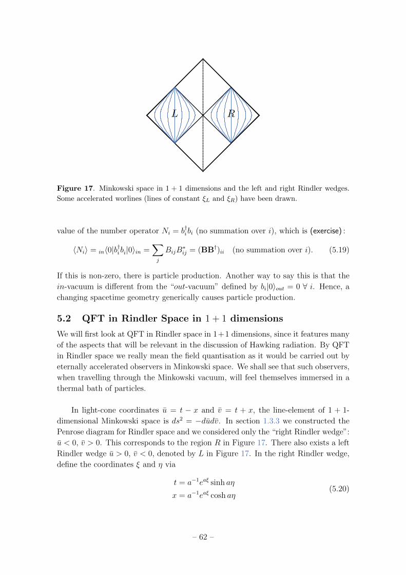
Figure 17. Minkowski space in 1 + 1 dimensions and the left and right Rindler wedges.
Some accelerated worlines (lines of constant ξL and ξR) have been drawn.
value of the number operator Ni = b†ibi (no summation over i), which is (exercise) :
〈Ni〉 = in〈0|b†ibi|0〉in =∑j
BijB∗ij = (BB†)ii (no summation over i). (5.19)
If this is non-zero, there is particle production. Another way to say this is that the
in-vacuum is different from the “out-vacuum” defined by bi|0〉out = 0 ∀ i. Hence, a
changing spacetime geometry generically causes particle production.
5.2 QFT in Rindler Space in 1 + 1 dimensions
We will first look at QFT in Rindler space in 1+1 dimensions, since it features many
of the aspects that will be relevant in the discussion of Hawking radiation. By QFT
in Rindler space we really mean the field quantisation as it would be carried out by
eternally accelerated observers in Minkowski space. We shall see that such observers,
when travelling through the Minkowski vacuum, will feel themselves immersed in a
thermal bath of particles.
In light-cone coordinates u = t − x and v = t + x, the line-element of 1 + 1-
dimensional Minkowski space is ds2 = −dudv. In section 1.3.3 we constructed the
Penrose diagram for Rindler space and we considered only the “right Rindler wedge”:
u < 0, v > 0. This corresponds to the region R in Figure 17. There also exists a left
Rindler wedge u > 0, v < 0, denoted by L in Figure 17. In the right Rindler wedge,
define the coordinates ξ and η via
t = a−1eaξ sinh aη
x = a−1eaξ cosh aη(5.20)
– 62 –

such that −∞ < ξ, η <∞ and
ds2 = e2aξ(−dη2 + dξ2). (5.21)
The proper time measured by a Rindler observer (i.e. along a ξ = const. line) is
τ = e2aξη if we synchronise it to τ = 0 as the observer passes the x-axis. Hence,
the coordinate η is a physical time-coordinate for the Rindler observer travelling at
constant ξ: it ticks at a rate proportional to the observer’s watch. Now define the
null coordinates u = η− ξ and v = η+ ξ, in terms of which the Rindler metric reads
ds2 = −e2aξdudv. (5.22)
The relation between the Minkowski and Rindler null coordinates is
u = −a−1e−au
v = a−1eav,(5.23)
which implies thatu→ 0 ⇐⇒ u→ +∞v → 0 ⇐⇒ v → −∞,
(5.24)
as shown in Figure 17. Notice the analogy to the relationship between the null
Eddington-Finkelstein coordinates (denoted above as u, v) and the Kruskal coordi-
nates U, V (1.25): U = −e−u/4M and V = ev/4M .
Analogous definitions can be made for coordinates that cover the left Rindler
wedge. The coordinates and line elements for the left and right Rindler wedge are
shown in table 2, where we’ve used subscripts to distinguish between the two wedges.
In this section, Rindler coordinates without subscript always refer to the right wedge.
In fact, the time coordinates ηL = ηR = tanh−1(t/x) are exactly the same func-
tion of Minkowski coordinates — they just take different ranges in L and R. We can
therefore drop the subscripts on η completely, as long as we remember that η < 0
corresponds to L and η > 0 to R. Lines of η = const. then correspond to lines
through the origin that extend over both L and R. These lines are Cauchy surfaces
for Minkowski spacetime. The vector ∂η is a timelike Killing vector (exercise) in both
L and R, but it is future-pointing in R and past-pointing in L. We now have three
globally hyperbolic manifolds with global future-pointing timelike Killing vectors:
Minkowski space with ∂t, the left Rindler wedge with −∂η, and the right Rindler
wedge with ∂η. In each of these the canonical quantisation procedure outlined in the
preceding section can be applied.
– 63 –
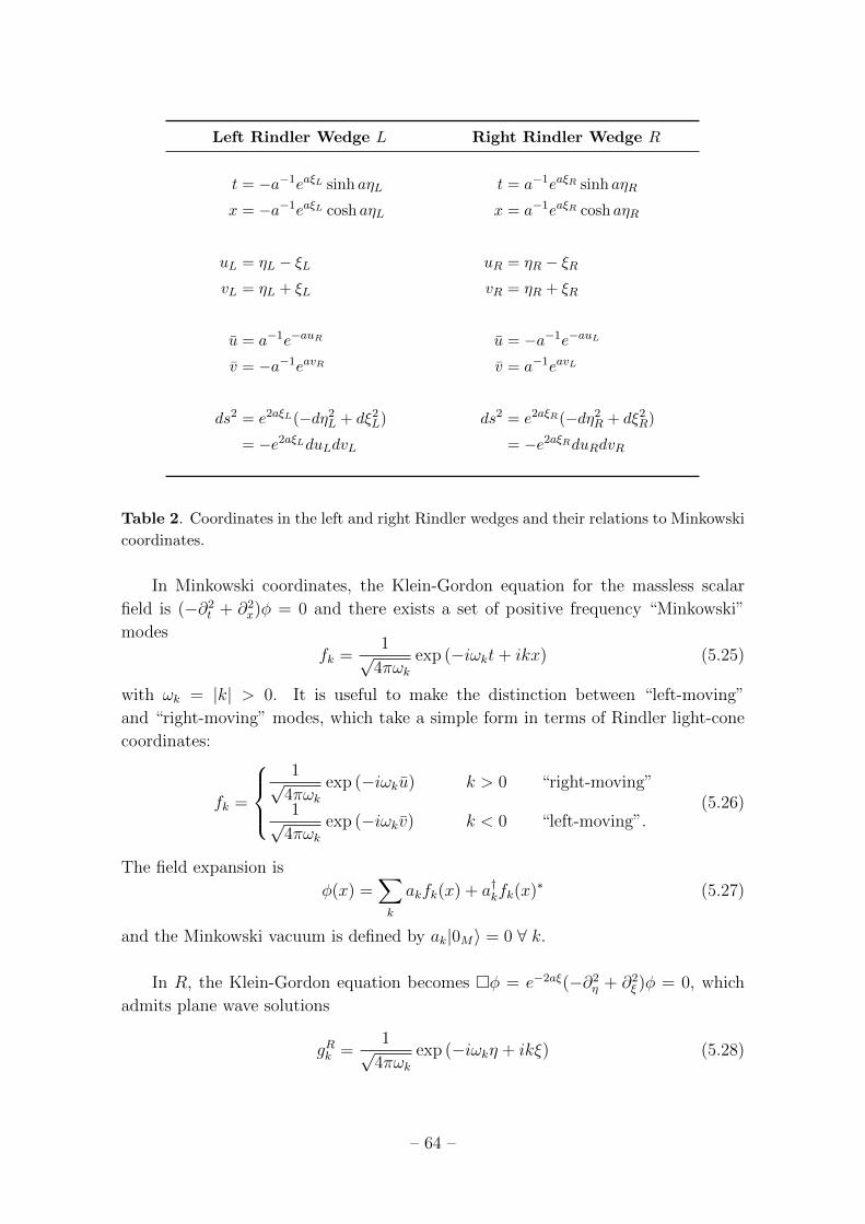
Left Rindler Wedge L Right Rindler Wedge R
t = −a−1eaξL sinh aηL
x = −a−1eaξL cosh aηL
uL = ηL − ξLvL = ηL + ξL
u = a−1e−auR
v = −a−1eavR
ds2 = e2aξL(−dη2L + dξ2
L)
= −e2aξLduLdvL
t = a−1eaξR sinh aηR
x = a−1eaξR cosh aηR
uR = ηR − ξRvR = ηR + ξR
u = −a−1e−auL
v = a−1eavL
ds2 = e2aξR(−dη2R + dξ2
R)
= −e2aξRduRdvR
Table 2. Coordinates in the left and right Rindler wedges and their relations to Minkowski
coordinates.
In Minkowski coordinates, the Klein-Gordon equation for the massless scalar
field is (−∂2t + ∂2
x)φ = 0 and there exists a set of positive frequency “Minkowski”
modes
fk =1√
4πωkexp (−iωkt+ ikx) (5.25)
with ωk = |k| > 0. It is useful to make the distinction between “left-moving”
and “right-moving” modes, which take a simple form in terms of Rindler light-cone
coordinates:
fk =
1√
4πωkexp (−iωku) k > 0 “right-moving”
1√4πωk
exp (−iωkv) k < 0 “left-moving”.(5.26)
The field expansion is
φ(x) =∑k
akfk(x) + a†kfk(x)∗ (5.27)
and the Minkowski vacuum is defined by ak|0M〉 = 0 ∀ k.
In R, the Klein-Gordon equation becomes φ = e−2aξ(−∂2η + ∂2
ξ )φ = 0, which
admits plane wave solutions
gRk =1√
4πωkexp (−iωkη + ikξ) (5.28)
– 64 –
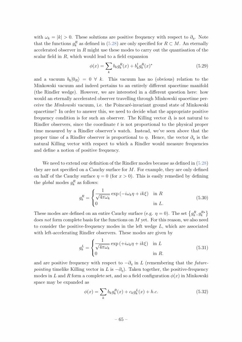
with ωk = |k| > 0. These solutions are positive frequency with respect to ∂η. Note
that the functions gRk as defined in (5.28) are only specified for R ⊂M . An eternally
accelerated observer in R might use these modes to carry out the quantisation of the
scalar field in R, which would lead to a field expansion
φ(x) =∑k
bkgRk (x) + b†kg
Rk (x)∗ (5.29)
and a vacuum bk|0R〉 = 0 ∀ k. This vacuum has no (obvious) relation to the
Minkowski vacuum and indeed pertains to an entirely different spacetime manifold
(the Rindler wedge). However, we are interested in a different question here: how
would an eternally accelerated observer travelling through Minkowski spacetime per-
ceive the Minkowski vacuum, i.e. the Poincare-invariant ground state of Minkowski
spacetime? In order to answer this, we need to decide what the appropriate positive
frequency condition is for such an observer. The Killing vector ∂t is not natural to
Rindler observers, since the coordinate t is not proportional to the physical proper
time measured by a Rindler observer’s watch. Instead, we’ve seen above that the
proper time of a Rindler observer is proportional to η. Hence, the vector ∂η is the
natural Killing vector with respect to which a Rindler would measure frequencies
and define a notion of positive frequency.
We need to extend our definition of the Rindler modes because as defined in (5.28)
they are not specified on a Cauchy surface for M . For example, they are only defined
on half of the Cauchy surface η = 0 (for x > 0). This is easily remedied by defining
the global modes gRk as follows:
gRk =
1√
4πωkexp (−iωkη + ikξ) in R
0 in L.(5.30)
These modes are defined on an entire Cauchy surface (e.g. η = 0). The setgRk , g
R∗k
does not form complete basis for the functions onM yet. For this reason, we also need
to consider the positive-frequency modes in the left wedge L, which are associated
with left-accelerating Rindler observers. These modes are given by
gLk =
1√
4πωkexp (+iωkη + ikξ) in L
0 in R.(5.31)
and are positive frequency with respect to −∂η in L (remembering that the future-
pointing timelike Killing vector in L is −∂η). Taken together, the positive-frequency
modes in L and R form a complete set, and so a field configuration φ(x) in Minkowski
space may be expanded as
φ(x) =∑k
bkgRk (x) + ckg
Lk (x) + h.c. (5.32)
– 65 –
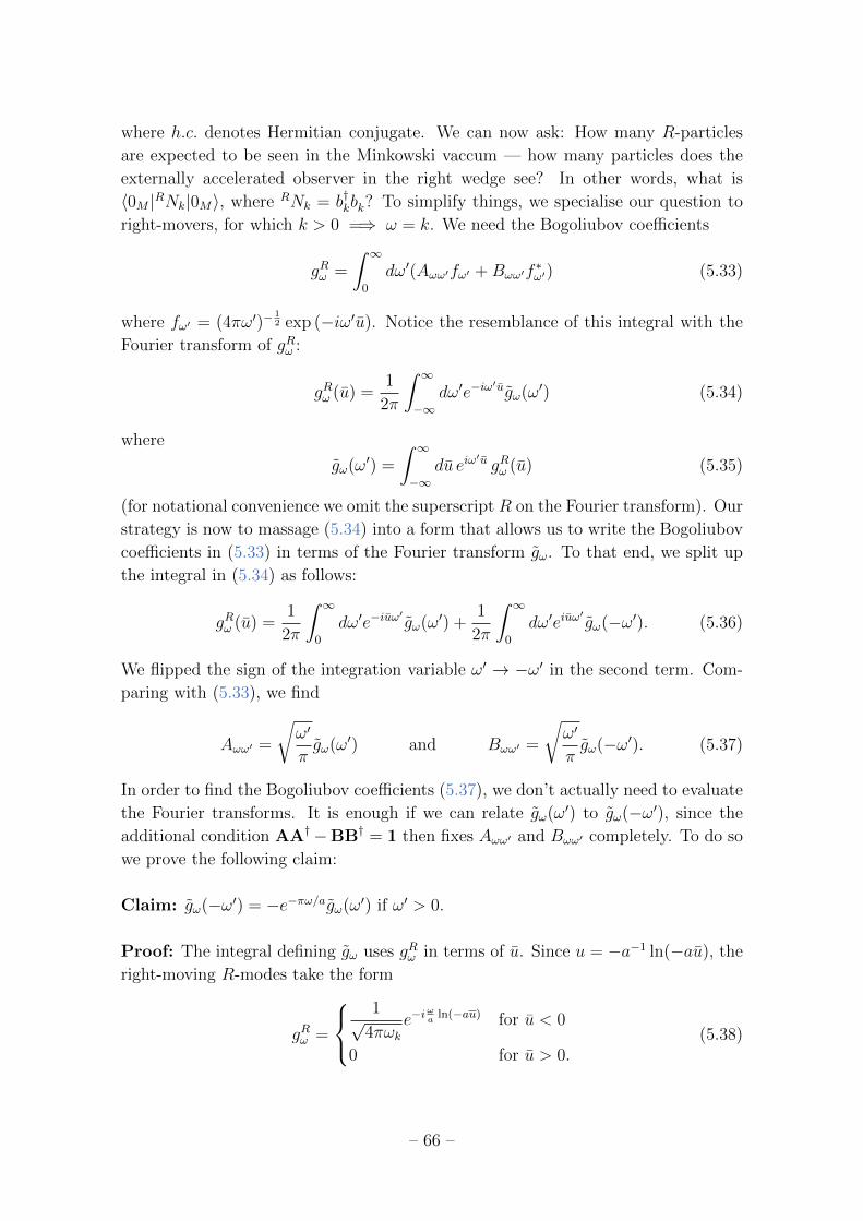
where h.c. denotes Hermitian conjugate. We can now ask: How many R-particles
are expected to be seen in the Minkowski vaccum — how many particles does the
externally accelerated observer in the right wedge see? In other words, what is
〈0M |RNk|0M〉, where RNk = b†kbk? To simplify things, we specialise our question to
right-movers, for which k > 0 =⇒ ω = k. We need the Bogoliubov coefficients
gRω =
∫ ∞0
dω′(Aωω′fω′ +Bωω′f∗ω′) (5.33)
where fω′ = (4πω′)−12 exp (−iω′u). Notice the resemblance of this integral with the
Fourier transform of gRω :
gRω (u) =1
2π
∫ ∞−∞
dω′e−iω′ugω(ω′) (5.34)
where
gω(ω′) =
∫ ∞−∞
du eiω′u gRω (u) (5.35)
(for notational convenience we omit the superscript R on the Fourier transform). Our
strategy is now to massage (5.34) into a form that allows us to write the Bogoliubov
coefficients in (5.33) in terms of the Fourier transform gω. To that end, we split up
the integral in (5.34) as follows:
gRω (u) =1
2π
∫ ∞0
dω′e−iuω′gω(ω′) +
1
2π
∫ ∞0
dω′eiuω′gω(−ω′). (5.36)
We flipped the sign of the integration variable ω′ → −ω′ in the second term. Com-
paring with (5.33), we find
Aωω′ =
√ω′
πgω(ω′) and Bωω′ =
√ω′
πgω(−ω′). (5.37)
In order to find the Bogoliubov coefficients (5.37), we don’t actually need to evaluate
the Fourier transforms. It is enough if we can relate gω(ω′) to gω(−ω′), since the
additional condition AA†−BB† = 1 then fixes Aωω′ and Bωω′ completely. To do so
we prove the following claim:
Claim: gω(−ω′) = −e−πω/agω(ω′) if ω′ > 0.
Proof: The integral defining gω uses gRω in terms of u. Since u = −a−1 ln(−au), the
right-moving R-modes take the form
gRω =
1√
4πωke−i
ωa
ln(−au) for u < 0
0 for u > 0.(5.38)
– 66 –

Figure 18. The contour integral used in the evaluation of gRω (−ω′) with a branch cut of
ln(−z) on the positive real axis.
The function ln(−z) is multi-valued on the complex plane so we will give it a branch
cut on the positive real axis. Then
gω(−ω′) =
∫ ∞−∞
du e−iω′ugω(u)
=1√4πω
∫ 0
−∞du e−iω
′ue−iωa
ln(−au).
(5.39)
Now we deform the path of integration, using the contour shown in Figure 18. The
contour is closed in the upper complex half-plane because the integral over the arc
segment C then vanishes for ω′ > 0 in the limit as the radius of the arc goes to infinity.
In order to avoid the branch cut we choose γ2 to lie just above the real axis by an
infinitesimal amount iε (which we send to zero at the end). Since the integrand has
no poles inside the closed contour (i.e. it is holomorphic there), Cauchy’s integral
theorem implies
0 =
∮du e−iω
′ue−iωa
ln(−au) =
∫γ1
+
∫γ2
+
∫C
du e−iω
′ue−iωa
ln(−au). (5.40)
Strictly speaking, there is another contribution on the right hand side for the integral
from iε to 0 (see Figure 18), but this will vanish when we send ε to zero at the end
so we can forget about it here. Since the integral over the arc C vanishes, it follows
– 67 –

from (5.40) that∫γ1
= −∫γ2
, which implies
gω(−ω′) = − 1√4πω
∫ ∞+iε
iε
du e−iω′ue−i
ωa
ln(−au)
= − 1√4πω
∫ −iε−∞−iε
du eiω′ue−i
ωa
ln(au) (u↔ −u)
= − 1√4πω
∫ 0
−∞du eiω
′ue−iωa
[ln(−au)−iπ] (ε→ 0)
= −e−πω/agω(ω′)
(5.41)
as claimed.
Hence we have Aωω′ = −e−πω/aBωω′ , which together with |Aωω|2 − |Bωω|2 = 1
implies
〈0M |RNω|0M〉 = (BB†)ωω = |Bωω|2 =1
e2πω/a − 1. (5.42)
This corresponds to a Planck spectrum with temperature T = ~a2πkB
.
In fact, we can show more: the state |0M〉 is the thermal state with respect to
the Rindler Hamiltonian HR, i.e. the Hamiltonian associated with a hypersurface
η = const. in the right Rindler wedge (in other words, HR generates time-translations
along ∂η). Mathematically this statement is
TrL (|0M〉〈0M |) =e−βHR
〈e−βHR〉(5.43)
where β = (kbT )−1 = 2πkb/~a. To show this, it is convenient to introduce so-called
Unruh modes, which are positive frequency with respect to ∂t, i.e. they are linear
combinations of fk-modes. The Unruh mode of frequency k is defined as
zk =1√
2 sinhωπ/a
(eπω/2a gRk + e−πω/2a gL−k
). (5.44)
In order to form a complete set, they must be complemented by the modes
z′k =1√
2 sinhωπ/a
(e−πω/2a gR−k + eπω/2a gLk
). (5.45)
The modes zk and z′k together with their complex conjugates form a complete basis
for functions on Minkowski space. Hence, the field can be equally well expanded in
terms of them:
φ(x) =∑k
dkzk(x) + d ′kz′k(x) + h.c. (5.46)
– 68 –

Comparing this with (5.32) we can read off
bk =1√
2 sinhωπ/a
(eπω/2adk + e−πω/2ad ′ †−k
)ck =
1√2 sinhωπ/a
(eπω/2ad ′k + e−πω/2ad †−k
) (5.47)
Since the Unruh modes are positive frequency with respect to ∂t, the Minkowski
vacuum satisfies dk|0M〉 = d ′k|0M〉 = 0 ∀ k. Now define the Rindler vacuum |0Rd〉by ck|0Rd〉 = bk|0Rd〉 = 0 ∀ k and further the (unnormalised) left- and right-wedge
n-particle states∣∣Rn, k⟩ = (b†k)n |0Rd〉 and
∣∣Ln, k⟩ = (c†k)n |0Rd〉 . (5.48)
Then it can be shown that
|0M〉 =∏k
(coshφk)−1
∞∑n=0
e−nπω/a∣∣Rn, k⟩ ∣∣Ln, k⟩ (5.49)
where φk is defined by tanhφk = e−πω/a. This state is perfectly entangled between
the left and right Rindler wedges: if a measurement is done in R in which n right-
wedge particles are found, then we know with certainty that the post-measurement
state has n left-wedge particles. To find the state ρR in R, we need to trace over the
states in L via the “partial trace” TrL. Defining En = nω, we obtain
ρR = TrL |0M〉 〈0M | =∞∑n=0
∏k
e−βEn∑∞m=0 e
−βEm
∣∣Rn, k⟩ ⟨Rn, k∣∣ =e−βHR
〈e−βHR〉(5.50)
as claimed above. This reveals something perhaps surprising about the Minkowski
vacuum: it is not a local quantity at all, i.e. it is not a state of the form
(vacuum at x1)⊗ (vacuum at x2)⊗ (vacuum at x3)⊗ . . .
Instead, it is a highly entangled state whose fluctuations are correlated throughout
spacetime.
The actual physical meaning of the results above may perhaps seem a bit ob-
scure. We considered the quantisation of a quantum field “appropriate to a Rindler
observer” in Minkowski space, which led us to conclude that a Rindler observer is
immersed in a thermal bath of radiation. How convincing were our arguments for
choosing some appropriate quantisation scheme? How would an eternally accelerated
observer actually measure the radiation? To put the results derived above on more
solid grounds, Bill Unruh constructed a simple model of a detector (nowadays known
as an Unruh-deWitt detector) and showed that an accelerated detector in Minkowski
space behaves as if it were in a thermal bath of particles. This effect is known as the
Unruh effect. Hawking radiation, which we discuss next, is a phenomenon closely
related to this effect.
– 69 –

5.3 QFT in the spacetime of a spherical collapsing star:
Hawking Radiation
Consider the spacetime that corresponds to a spherically symmetric collapsing star,
heavy enough to form a black hole. The Penrose diagram is shown in Figure 19.
This is a curved spacetime that is globally hyperbolic (for instance J − is a Cauchy
surface). Even though the Schwarzschild black hole solution is a static spacetime, the
collapsing star spacetime is not : the formation of the black hole involves complicated
dynamics. However, the spacetime is approximately stationary in the far asymptotic
past (i.e. near J −) and in the far asymptotic future (i.e. near J +). Therefore
we can perform a second quantisation associated with stationary observers near J −(which leads to the so-called in-vacuum), and a second quantisation associated with
stationary observers near J +. We can then ask the question we asked in the example
of the “sandwich spacetime” above: will observers in the far future see particles in
the in-vacuum?
The field expansion defining the in-vacuum can be constructed by specifying
a complete set of positive-frequency modes on J −. For the quantisation in the far
future, it is not sufficient to define a complete set on J +, because J + is not a Cauchy
surface for the spacetime (for example, causal curves that end on the singularity
never register on J +). However, the surface H+∪J + is a Cauchy surface, so we can
quantise the field in the far future by specifying a complete set on it. Hence there
will be three sets of modes:
fi : positive frequency on J −
gi : positive frequency on J + and zero on H+
hi : positive frequency on H+ and zero on J +.
(5.51)
(Strictly speaking, there is no timelike Killing vector on H+ — recall that ∂t is null
on the horizon — so the term “positive frequency” is somewhat misleading there.
However, the outcome of the calculation does not actually depend on the choice of
modes hi, so we can just choose an arbitrary set of modes on H+ and declare those
as the “positive frequency” modes, i.e. attach them to annihilation operators in the
field expansion, as long as together with gi they form a complete set. For more detail,
see Wald §14.3.) The set fi, f ∗i is complete. The sets gi, g∗i and hi, h∗i are not
complete by themselves but together they form a complete set. We can expand the
field in two ways:
φ(x) =∑i
aifi(x) + h.c. =∑i
bigi(x) + cihi(x) + h.c. (5.52)
As before, to find out what observers at late times on J + see in the state |0in〉defined by ai |0in〉 = 0 ∀ i, we will evaluate 〈Ni〉 = (BB†)ii, for which we need the
– 70 –

Figure 19. Penrose diagram of the spherically symmetric collapsing star.
Bogoliubov coefficients in the expansion
gi =∑j
Aijfj +Bijf∗j . (5.53)
If we could find the exact solutions to the Klein-Gordon equation, this would
be a fairly straight-forward task: once the positive-frequency solutions gi on J + are
specified, we can do the analog of a Fourier transform to find their expansion in terms
of fi and f ∗i on J − (such an expansion always exists since fi, f ∗i is a complete set
of functions) and read off the Bogoliubov coefficients. However, we will see in a
moment that the Klein-Gordon equation is complicated in Schwarzschild spacetime,
which prevents us from finding analytic solutions. Instead, we will ask: if a given
solution to the Klein-Gordon equation is asymptotically positive-frequency at J +,
then what is its form at J −? In other words, we will impose a boundary condition
to the solution at J + and investigate what its corresponding form must be on J −.
This amounts to “tracing back in time” the solution from J + to J −.
The metric of the Schwarschild black hole spacetime with coordinates (t, r∗, θ, φ)
reads
ds2 =
(1− 2M
r
)(−dt2 + dr2
∗) + r2dΩ22. (5.54)
We will also use the light-cone coordinates u = t − r∗ and v = t + r∗ below. Using
the handy formula
= ∇µ∇µ =1√−g
∂µ(√−ggµν∂ν
)(5.55)
we can find the Klein-Gordon equation for the field φ(t, r∗, θ, φ). Expanding the
solution in spherical harmonics φ(t, r∗, θ, φ) = χl(r∗, t)Ylm(θ, φ) we find[∂2t − ∂2
r∗ + Vl(r∗)]χl = 0 (5.56)
– 71 –

Figure 20. The potential Vl as a function of r∗ (shown here for l = 1).
where
Vl(r∗) =
(1− 2M
r
)[l(l + 1)
r2+
2M
r3
]. (5.57)
Set χl(r∗, t) = e−iωtRlω(r∗) so that
(∂2r∗ + ω2)Rωl = VlRωl. (5.58)
This equation can be cast into a form known as the confluent Heun equation, whose
solutions have been studied to some extent but are complicated. We can gain some
insight into the solutions by looking more closely at the potential Vl(r∗). Both near
the horizon H+ (r → 2M ⇐⇒ r∗ → −∞) and near J ± (r → ∞ ⇐⇒ r∗ → ∞),
the potential tends to zero — it takes the form of a potential barrier, as shown in
Figure 20. Hence, if we consider how any particular solution to (5.58) evolves in
time, it will be partly transmitted and partly reflected as it comes in from r∗ =∞.
Near J ±, the solutions to (5.56) are just plane waves. The equivalent of right-
moving and left-moving for a radial coordinate is outgoing and ingoing (correspond-
ing, respectively, to r∗ increasing or decreasing with time) so we define “early modes”
flmω+ =1√2πω
e−iωuYlmr
(outgoing)
flmω− =1√2πω
e−iωvYlmr
(ingoing)
(5.59)
at J −, and “late modes”
glmω+ =1√2πω
e−iωuYlmr
(outgoing)
glmω− =1√2πω
e−iωvYlmr
(ingoing)
(5.60)
– 72 –

at J +. We will be interested mainly in ingoing early modes and outgoing late modes,
so we will use the shorthand notation
fω ∼ flmω−
gω ∼ glmω+.(5.61)
We need to express gω in terms of fω′ and f ∗ω′ on J −. First, note that plane waves
such as gω are in fact completely delocalised, i.e. they have support everywhere on
J +. However, using a superposition of such positive frequency plane waves, we can
always construct a localised “wave packet” on J + (for example a Gaussian packet)
and we can choose it to be peaked around some momentum ω0 and around some
coordinate value u0. Hence, when we speak of the “outgoing mode at late times” we
really mean a linear combination of outgoing modes on J +. Keeping this in mind,
we phrase our argument below in terms gω for simplicity.
In order to find the expansion of the late mode in terms of early modes, we can
trace the solution back in time. As the wave travels inwards from J + (toward de-
creasing values of r∗), it will encounter the potential barrier. One part of the wave,
call it g(r)ω , will be reflected and end up on J − with the same frequency ω. This
will correspond to a term of the form Aωω′ ∝ δ(ω − ω′) in (5.53). The remaining
part g(t)ω of gω will be transmitted through the barrier and will enter the collapsing
matter. In that region, the precise geometry of spacetime is unknown. However,
since we are interested in a packet peaked at late times (i.e. large u0) and at some
finite frequency ω0, we know that the packet will be peaked at a very high frequency
as it enters the collapsing matter due to the gravitational blueshift. This leads to an
important simplification: the packet will obey the geometric optics approximation,
which means that gω takes the form A(x)eiS(x) where A(x) is slowly varying com-
pared to S. Substituting this into the Klein-Gordon equation gives ∇µS∇µS = 0,
which means that surfaces of constant phase are null. Given a wave, we can therefore
trace its surfaces of constant phase back in time by following null geodesics.
Consider tracing back the wave along a particular null geodesic γ which starts
off at some u = u0 at J + and hits J − at v = v0. as in Figure 21. We denote
by γH a null generator of the horizon H+, which has been extended into the past
until it hits J − at some value of v. We may set this value to v = 0 without loss
of generality, since the spacetime is invariant under shifts v → v + c. In that case
we have v0 < 0 for the geodesic γ. Let n be a connecting vector between the two
curves as shown in Figure 21. Fix its normalisation by requiring n.` = −1, where `
is a generator of the Killing horizon H+. Near the horizon, the Kruskal coordinate
U = −e−κu is an affine distance along n and we can use it to measure the distance
between γ and γH (1.25). In order to find the form of the wave at J −, we need to
understand how the affine distance along the connecting vector n will change by the
– 73 –

Figure 21. The BLA.
time γ reaches J −. At J −, the coordinate v is an affine parameter along the null
geodesic integral curves of n. If U0 = 0 (corresponding to u0 = ∞) then the affine
distance is zero at J −. Hence we can expand the affine distance between γ and γHat J − in powers of U0: v = cU0 + O(U2
0 ) for some constant c > 0 (since U, v < 0).
Using u = −κ−1 ln(−U) = −κ−1 ln(−cv), we can conclude that if a mode takes the
form gω ∼ e−iωu on J +, the transmitted part g(t)ω on J − will take the form
g(t)ω ∼
eiωκ
ln(−v) for v < 0
0 for v > 0(5.62)
up to a constant phase. This is exactly analogous to the Rindler modes in the
previous section, with κ↔ a. We have Aωω′ = e−πω/κBωω′ and therefore
〈Nω〉 ∝1
e~ω/kBT − 1(5.63)
where the Hawking temperature is given by T = ~κ2πkB
. Since this temperature is
inversely proportional to the mass, the black hole heats up as it evaporates.
– 74 –