Biscayne Bay Water Quality Monitoring Networka definition of “hot spots” be developed to guide future optimal monitoring program designs for these regions. 2. Laboratory Inter-Comparison

_____________________________________________________________________________________ February 2006 1

Biscayne Bay Water Quality Monitoring Network

Optimization Leader: Carlton D. Hunt, Battelle Statistician: Fred Todt, Battelle

Project Code: BISC Mandate/Permit:

• Biscayne Bay Minimum Flows and Levels (MFL) • CERP Implementation (Biscayne Bay Coastal Wetlands Project, C-111 Spreader Project, Wastewater

Reuse Project, RECOVER Monitoring and Assessment Plan) • Water Reservations (under Acceler8 and CERP) • Clean Water Act (TMDL development) and Florida Statues (373.4595), mandates for protecting

Outstanding Florida Waters (non-degradation standard) and tracking trends. • Biscayne Bay SWIM Plan

Project Start Date: 1978 began, was updated in 1995 Division Manager: Coastal Division: Sean Sculley (Acting) Program Manager: Dave Rudnick Points of Contact: Dave Rudnick, Trisha Stone, Teresa Coley, Braham Charkian Field Point of Contact: Braham Charkian Spatial Description: The monitoring program includes all of Biscayne Bay from the Broward County line to U.S. Highway 1 at Key Largo and tributaries to Biscayne Bay. Several District canals empty into Biscayne Bay. Monitoring sites are fixed and are denser in the northern area of the bay than the southern area. The program covers roughly 1400 square miles. Two water quality monitoring contracts support the District’s management of the Biscayne Bay region, one with Miami-Dade DERM and one with FIU. The FIU Biscayne Bay project was optimized during a previous effort. District staff suggested that the FIU information be evaluated with the DERM data for this BISC optimization. In addition to spatial redundancies, frequency of sampling and the parameters that are sampled by both organizations should be compared to determine if redundancies or data gaps exist. Project Purpose, Goals and Objectives: Project BISC serves the mandates listed above. The District and DERM initiated and maintained this monitoring program to identify areas of ecological concern and provide a clear understanding of baseline conditions using both systematic and investigative monitoring. The main purpose has been to characterize water quality spatially and seasonally, and to detect long term trends. Additionally, the program has also been used to identify specific hotspots, develop and monitor comprehensive stormwater improvement programs, develop non-degradation criteria, and develop freshwater response relationships. An objective of the program is to maintain the long term dataset for characterization of water quality through various climatic cycles, events and watershed changes. DERM data is used to address Dade County water quality permitting issues and support various non degradation and TMDL planning activities for Biscayne Bay. As such the focus of DERM’s sampling is in canals; DERM’s Bay sampling

_____________________________________________________________________________________ February 2006 2

program is on receiving waters with a focus on channels. Several DERM stations are named in RECOVER’s Monitoring and Assessment Plan (MAP) as key stations for assessment of environmental response to the CERP. FIU data is used to support long term water quality assessments and planning. The FIU stations purposely avoid sampling in channels in Northern Biscayne Bay. Funding for the DERM program comes from the State of Florida through the District, while funding for FIU originates with the District. Sampling Frequency and Parameters Sampled: Samples are collected via grab from numerous stations at varying frequencies (see parameters measured tables). The metals cadmium, copper, lead and zinc as well as total suspended solids are sampled quarterly by DERM. DERM also samples for Chlorophyll a, color, turbidity, total Kjeldahl nitrogen and orthophosphorus bimonthly while coliforms (total and fecal) and the remaining nutrients (ammonia, nitrite+nitrate [NOx], and total phosphorus) are sampled monthly. DERM only samples for hardness and TKN at stations upstream of salinity control structures. In situ measurements are taken at all sampling locations monthly. These measurements include dissolved oxygen, pH, water temperature, specific conductance, salinity and photosynthetically active radiation (PAR). The sample depth and total depth of the water column is also recorded at all sampling stations. The optimization review process ascertained that the acronym TP used in the original monitoring plan summary table was misnamed and should be called TPO4 (DBHydro code 25) and is the accurate parameter describing total phosphorous. TP is listed in DBHyro as code 101 and refers to particulate phosphorus. This should be clarified in the District’s monitoring plan. FIU samples the marine portion of the study area for all parameters listed in its monitoring program monthly. The optimization identified that TOTN is monitored monthly by FIU; this parameter has been added to the FIU parameter table. Current and Future Data Uses: The primary uses of the program data by SFWMD are to develop minimum flows and levels (MFL) technical criteria using the salinity values, evaluate targets and performance measures for CERP using salinity and nutrients, setting permit criteria for District projects, and reporting trends in the Biscayne Bay section of the annual South Florida Environmental Report (SFER). Thirty-two of the DERM stations are identified as key stations for monitoring Biscayne Bay by RECOVER (RECOVER, 204). All but two of the RECOVER samples are listed as Type II stations. Stations BB50 and PR01 are listed as Type III stations. Miami Dade DERM uses the data in ways that indirectly benefit the SFWMD’s mission. For example, the data are used to calibrate and verify stormwater management models, prioritize basins for non-point source control and identify and investigate pollution sources to Biscayne Bay. This project also supports District funded stormwater improvement projects throughout the watershed. In addition, research projects funded by SFWMD use some of the data in comparative analysis. In the future, results from this program are expected to support assessment of MFL, permit criteria, and the effectiveness of specific CERP projects including general water quality trends that may be attributed to implementation of CERP (including C-111 Spreader Canal, Biscayne Bay Coastal Wetlands and the Wastewater Re-use Study). One example is monitoring the water quality discharged from the Biscayne Bay Coastal Wetlands Project (includes an Acceler8 component) to test expected load reduction targets. The RECOVER Monitoring and Assessment plan will use many of the sites for long-term monitoring. Data from the project will also support development of TMDLs, PLRGs and will be necessary for the Southern Coastal Biscayne Bay MFL. Examples of other organizations that will use the data in ways that benefit the SFWMD include FDEP’s TMDL program to identify impaired waters, and DERM’s development of a water quality model for Biscayne Bay (Biscayne Bay Feasibility Study II B).

_____________________________________________________________________________________ February 2006 3

Identified Optimization Opportunities: Discussions with District staff identified several potential opportunities for optimization. District staff felt it is necessary to evaluate both the FIU and DERM Biscayne Bay data together to better determine redundancies/data gaps in the spatial and temporal, and in the parameters sampled. District staff also indicated that because a single laboratory did not conduct laboratory analysis the optimization effort should evaluate the data from the two programs for potential analytical differences. District staff also voiced concern regarding the quality of the trace metals data from the estuarine environment and indicated the optimization effort should consider this. There was also concern regarding the extent of the DERM’s sampling upstream of the structures in the canals emptying into Biscayne Bay. District staff questioned whether there may be overlap with other District monitoring projects at these more interior locations. Some of the stations suggested for closer examination correspond to the following structures: S196, S194, S338, S333, S32, and G72. Comparative information was not developed under this project due to a reduction in the effort expended on evaluating the canals. District staff also suggested using a gradient-type optimization approach to evaluate whether there differences exist between the two programs at nearshore stations, mid-bay stations, or offshore stations. SFWMD personnel indicated the District may suggest improvements to the program that could be mutually beneficial to Miami-Dade County as a result of the optimization. In the past, most of these suggestions have included improvements to the quality assurance program, data management, adding stations and parameters. The largest gap identified has been the paucity of monitoring stations in nearshore southern Biscayne Bay. This was rectified to some extent previously when the County added stations to the network in the area. Other programs such as FIU’s regional monitoring program and Biscayne National Park’s monitoring have filled this gap to a great extent. In addition the Florida Bay monitoring program maintains several stations in this region under the FLAB program. A primary opportunity for improvement within the project is data availability. DERM maintains and updates its database regularly and makes data available on request. They also submit data to the District for inclusion in DBHydro. It is unclear how changes to the data necessitated by ongoing review and data evaluations by DERM and other users are transmitted to the District for corrective action. This can create issues relative to assessments as most current data may not be available to the users. For example, data verification efforts during the current optimization found several data updates made by DERM and carried in their database that had not been made in DBHydro. This raises questions regarding the most effective means of data storage, updates, and retrieval. Optimization analysis: The optimization analyses consisted of series of activities defined in the BISC optimization plan of June 2005 with subsequent modifications. These include 1) characterization of data uses by the program, 2) inter-laboratory data comparison to determine the comparability of the two laboratories conducting water quality monitoring in Biscayne Bay, 3) statistical evaluations to determine geographic domains in the Bay, 4) an evaluation of the spatial and temporal adequacy of the BISC Project with respect to trend detection in key water quality parameters by geographic domain within the Bay, 5) assessment of potential redundancies among stations, and 6) compilation of summary statistics for key parameters for each station in the 11 canals included in the Project.

_____________________________________________________________________________________ February 2006 4

1. Characterization of data uses The evaluation of the mandates and monitoring objectives for the two monitoring program deployed in Biscayne Bay identified twelve primary data uses (Appendix 1). However, optimization for each data use became problematic due to resource limitations. Therefore, the BISC optimization was restricted in scope to address the highest priorities. These were the inter-laboratory comparability of Bay data and the ability to detect trends as defined in the 10 year data record. The primary data uses addressed were:

A. Estimate baseline (e.g., conditions before a management action is implemented or data that defines the current conditions to include trends and spatial variability over the past several years) coastal water quality parameter concentrations for stations with common physical associations (e.g., definable geographic domains)

B. Detect changes in coastal water quality parameter concentrations that result from climatic

cycles, events, watershed changes (i.e. comprehensive storm water improvement programs) for stations with common physical associations

C. Detect changes resulting in the project area from alterations in freshwater source strengths and

hydrological changes. The identified data use “Enable documentation of changes in temporal and spatial trends of known “hotspots” in the system” was dropped from the optimization since the data investigation did not find any “hot spots” of substantial spatial or temporal scale that would allow optimization. It is recommended that a definition of “hot spots” be developed to guide future optimal monitoring program designs for these regions. 2. Laboratory Inter-Comparison The inter-laboratory comparison analysis was completed using stations from the two monitoring programs that were either co-located (four stations) or in close proximity (within a few hundred meters) of each other (six stations). Six parameters (Dissolved Oxygen (DO), salinity, nitrate plus nitrite (NOx), ammonia (NH4), total phosphorus (TPO4), and Chlorophyll a) appeared to have a sufficient amount of data for these comparisons over the period of record. Data from the two programs were compared using box plots, regression analysis, and temporal plots (See Appendix 2). The results of these analyses are summarized below:

A. Of the six parameters compared (salinity, dissolved oxygen, NOx, NH4, TPO4, and Chlorophyll a) only salinity and dissolved oxygen are reported for depths greater than 1m. Uncertainty in the comparisons was high because only four stations are co-located and temporal congruity in sampling times was limited.

B. Salinity, dissolved oxygen, NOx, and Chlorophyll a measured by the two programs had similar statistical characteristics for the period of record.

C. Ammonia did not display similar statistical characteristics due to differences in the analytical methods (total ammonia {unfiltered} [DERM] versus dissolved ammonia [FIU]).

D. Small differences in the TPO4 data were noted but the cause(s) were not identified. E. Regression analysis of co-located stations found reasonable correlation for salinity,

temperature, and dissolved oxygen between the two programs in spite of the large uncertainty in pairing the sample collection dates and time (e.g. only data collected within a 24h window could be compared).

_____________________________________________________________________________________ February 2006 5

F. Time series visualizations also suggest the two programs are reporting comparable salinity, chlorophyll, and dissolved oxygen data ranges.

Recommendations The comparison of the monitoring data from the two laboratories revealed several issues that go towards optimization of the monitoring program.

A. Four co-located stations are sampled for the same parameters (BB17 and BISC131; BB37 and BISC108; BB38 and BISC111; BB44 and BISC116). Depending on the objectives of each program, sampling of these stations by both programs can be considered redundant.

B. Sample collection depths are inconsistent between and within the two programs, particularly

samples obtained near the surface (0.1 or 1.0 m depth) and 1m and deeper. Both programs sample in situ parameters within a few centimeters of the water surface (<0.1m). Depending on the station, the FIU data below the surface were reported for a constant depth but that depth could be 2, 3, or 4.5 m below the water surface. DERM data from depth included samples from a fixed depth (1m) and from variable depths below 1m. The latter data were obtained from 1.5 to 5m.

C. The rationale for the selection of the depths was not evident in the available documentation.

For future monitoring, it is recommended that the rationale for collecting samples from depth be articulated and a consistent sample collection protocol be defined for the two monitoring programs to follow. This will ensure both the representativeness of the data and its comparability, resulting in a more consistent ability to assess system response.

D. The rationale for close spaced depth intervals (surface ~1m, 2m, etc.) is not clear. Depending

on Data Quality Objectives, the samples at intermediate depths could be eliminated from the experimental design.

E. Only 1 to 5 percent of the data collected from the co-located and close proximity stations was

sufficiently congruent in space and time to enable data comparison, thus regression analysis was of limited value. Most DERM and FIU sampling dates are separated by days, often weeks. Temporal plots indicate the data fall within the same range on long time scales.

F. The parameters measured and reported by the two programs in Biscayne Bay vary. For

example, both programs measure TPO4 in Biscayne Bay. However, TP was erroneously indicated as a DERM parameter (the measured parameter is TPO4). According to the database rules, TP conveys the concentration of phosphorous in particulate matter on a mass of phosphorous per unit of particulate mass basis (not a volume basis). Conversion of mass/mass units to mass/volume units requires TSS data (mass/volume). Also, DERM does not include a measure of total nitrogen in its coastal program, thus a comparison with FIU TOTN data was not possible. Moreover, color is not measured by FIU but is reported in the Bay by DERM. The value of color in the salt water domain, especially from offshore stations that are typically deep, is unclear.

G. The parameters measured at various stations also differ between the two programs. For

example, ammonia, NOx, and TPO4 are not measured at each DERM station in Biscayne Bay; rather a subset of stations is sampled and analyzed for these parameters. The rationale for

_____________________________________________________________________________________ February 2006 6

including each parameter in the programs should be clarified against mandate requirements and scientific rationale for both programs and reconciled where appropriate.

H. FIU has not included BISC105, 106, 107, 114, 115, 117, 118, 119, 120, and 125 in the

monitoring program since 1996. The reasons why were not evident in the documentation provided, although it is clear that Stations BISC105, 106, 107 represent ocean conditions (useful as boundary stations for water quality models) for central Biscayne Bay. This was confirmed through conversations with DERM and FIU Principal Investigators. The other stations were located in the southern Biscayne Bay and some such as BISC118 are in passages connecting the southern Bay to the open ocean. Reasons to add these stations back into the program were not evident at this stage of the optimization.

I. This comparison found that some parameters measured by the two programs could be included

in the optimization statistical analysis. These include salinity, dissolved oxygen, NOx, and chlorophyll, and TPO4. TPO4 data was included in the optimization even through methodological issues may cause small differences where low levels of TPO4 are encountered. Ammonia data could not be included in the optimization because the programs use fundamentally different ammonia measurements (i.e., DERM measures total ammonia [Zhang et al. 1997] versus FIU’s dissolved ammonia measurements [Caccia and Boyer 2005]).

3. Geographic Domain Identification The geographic domains were selected based on a cluster analysis (SAS PROC CLUSTER, Ward method which uses a Euclidean distance function to compute distances) of Biscayne Bay data from both programs. The cluster analyses used quarterly means of salinity and temperature data restricted to samples collected from the surface (<0.5m) and information included in recently published peer review papers (Caccia and Boyer 2005). Inclusion of other parameters and larger depth ranges were evaluated but not reported here. Several parameters were eliminated due to low sample numbers or poor comparability between the programs. Temperature, salinity, and dissolved oxygen provided the most robust data set over the longest period of record (12 quarters from spring 2000 through winter 2003). Depths were restricted to less than 0.5 m due unbalanced sampling depths in the two programs. An evaluation of redundancy between stations was also attempted using a Spearmans rank correlation analysis. However, the time interval between the sampling dates was too great to pair the station data, thus this analysis did not provide useful information and was not further pursued. Five geographic domains were identified within Biscayne Bay through the cluster analyses (Figure 1). See Appendix 3 for the dendogram and station assignment. The station sets associated with these geographic domains are shown in Table 1. Stations that have been identified in the MAP (Recover 2004) as key stations for RECOVER are highlighted. Because Caccia and Boyer (2005) did not find substantial seasonal effects in the same FIU ten-year data set, the combined DERM/FIU data were not subjected to seasonal cluster analysis. Discussions with DERM indicated that their stations are primarily located in navigation channels and that the seaward most canal stations are located seaward of any canal structure. These stations are designated with the canal’s acronym [e.g., SK-] and -01. Because these stations are heavily influenced by the ocean, they were included with the along shore and northern Biscayne Bay geographic domains for statistical trend testing. Most of the DERM central and southern Biscayne Bay are located along and near the shore in regions most heavily influenced by canal discharges.

_____________________________________________________________________________________ February 2006 7

Figure 1. Geographic domains in Biscayne Bay based on the 12 quarter, two parameter (salinity and temperature), <0.5m cluster analysis that explain 81 percent of variability in the data.

_____________________________________________________________________________________ February 2006 8

Table 1. Geographic domains and associated stations based on the 12 quarter, two parameter (salinity and temperature), <0.5m cluster analysis. Stations in Biscayne Bay identified in the MAP as key to this program are highlighted.

Geographic Domain

DERM Stations FIU Stations Description Comments

Northern Biscayne Bay

BB03, BB04, BB05A, BB06, BB07; BB09, BB10, BB11, BB14, BB15; BB16, BB17, BB18, BB19, BB22, BB23, BB24, BB25, BB26, BB27, BB28, BB54, SK01, AC01, BS01, LR01, MR01

BISC129, BISC130, BISC131, BISC132, BISC133, BISC134

SK area to Bear Cut

DERM = 26 FIU = 6 Total = 32

West Central Biscayne Bay (along shore)

BB39A; BB52, BB53; MW01; MI01, GL02, BL01, CD01A, PR01

BISC101, BISC102, BISC103

Along shore in proximity with major fresh water discharge locations


Intermediate Biscayne Bay

BB29, BB31, BB32, BB34, BB41, BB36, CG01, SP01

BISC110, BISC123, BISC122, BISC126, BISC127, BISC128

Near shore area extending from north to south through out central and southern central Biscayne Bay,


Offshore Central Biscayne Bay

BB38, BB44, BB35, BB37

BISC104, BISC108, BISC109, BISC111, BISC112, BISC113, BISC116, BISC124

Region in central and south central Biscayne Bay seaward of the Intermediate domain.


Southern Biscayne Bay

BB45, BB47, BB48, BB50, BB51;AR01,

BISC121, BISC135

Manatee Bay, Card Sound and Barnes Sound; Four FLAB stations are called for in the MAP

DERM = 6 FIU = 2 Total = 8 Some may associate with intermediate

_____________________________________________________________________________________ February 2006 9

4. Trend Detection in Water Quality Parameters The parameters identified for statistical optimization of the Biscayne Bay sampling program were: salinity (98), dissolved oxygen (8), TOTN (80), TPO4 (25), and Chlorophyll (61). The DBHydro method numbers are identified in the parenthesis. These parameters are measured under both programs conducting Biscayne Bay monitoring, except TOTN, which is measured only by FIU. Statistical analysis and optimization of metals, bacterial indicators, and several parameters measured to support the programs objectives were conducted. Review of the available data suggests the metals and bacterial indicator parameters may be over sampled in parts of the Bay, particularly in the offshore regions most influenced by the ocean boundary of the Bay. Comparison of the sample collection frequencies and depths for the two programs found the programs were reasonably consistent in the sampling frequency and depths (surface samples from <0.1m) but the sampling times in any given month did not match closely. Even so only 1 to 5% of the data used in the inter-laboratory regression analyses were obtained within 24 hours of each other and at the same depth. More often, the sample collection dates were separated by days, often weeks. Thus, the two programs together represent a higher frequency sampling effort than when a program is considered individually. It was also identified that the in situ data has the highest rate of data collection across the station sets. For several parameters, the DERM program selectively samples the Bay from both spatial and temporal perspectives for those parameters measure in laboratories. Based on this the two data sets were combined to determine the base case for conducting trend analysis. The optimization assessed the power to detect trends for the five water quality parameters selected for optimization. Monte Carlo simulations were performed using the seasonal Kendall Tau Test for trend. The details of this statistical approach can be found in Rust (2005). The steps and code were provided to the District as a tool for use in further optimizations. The power analyses was used to determine the smallest water quality trends that will be detectable with high probability based on water quality data collected according to current monitoring plans. The power analyses were performed by carrying out the following power analysis steps for each geographic region-parameter combination. The combined data from the two monitoring programs were regionally average into 15-day periods for the base case

• Fit a statistical model to the water quality parameter data in order to have a basis for generating simulated data to support a Monte Carlo based power analysis procedure

• Generate multiple replicate simulated water quality time series data sets; for all power analyses

reported here, each time series generated was for a 5-year monitoring period • Perform a Mann-Kendall trend analysis procedure (Reckhow et al. 1993) for each simulated time

series data set; in particular, obtain a point estimate of the slope vs. time for the log-transformed water quality parameter values

• Estimate the annual proportion change (APC) in water quality parameter values that is detectable

with 80% power using a simple two-sided test based on the Mann-Kendall slope estimate performed at a 5% significance level

Parameter values were natural log-transformed for statistical modeling because the log-transformed data was more nearly normally distributed than were the untransformed data. The fitted statistical model contains the following components:

_____________________________________________________________________________________ February 2006 10

• Fixed seasonal effects that repeat themselves in an annual cycle • A long-term linear trend in the log-transformed parameter concentrations; this corresponds to a

fixed percentage increase or decrease in the water quality parameter each year

• A random error term representing temporal variability in true water quality parameter values; these error terms are allowed to be correlated from one time point to the next in order to capture any serial autocorrelation that is present in the monitoring data

• A random error term representing sampling and chemical analysis variability; these error terms are

assumed to be stochastically independent from one time point to the next The fitted statistical model is used to perform a Monte Carlo simulation analysis in which multiple time series data sets are simulated and used to determine the anticipated statistical properties of trend detection procedures that will be used by the District. All statistical trend analyses performed on the simulated data were based on the Mann-Kendall trend analysis procedure (Reckhow et al. 1993) preferred by the District. In the course of performing the power analyses for the District, it was determined that the basic Mann-Kendall trend detection procedures do not necessarily control the true significance level of the hypothesis test for trend when there is serial autocorrelation exhibited in the data. This was found to be true even for procedures that attempt to correct for serial autocorrelation. For this reason, all power analysis results reported here are for a simple hypothesis test procedure based on the median slope estimator that accompanies the Mann-Kendall test procedure. The median slope estimator is assumed to follow a normal distribution and power results are obtained by performing a simple z-test with this estimator. In summary, the approach entailed using the simulations to provide an estimate of the slope (time series trend) that can be detected under the current spatial and temporal program design as well as alternative temporal designs. A target slope equivalent to an annual percent change (APC) of 20 in any given parameter over a five year time period was used. The APC was calculated for each monitoring scenario. For the analyses, an APC of les than means the data has the ability to detect smaller changes. Conversely a higher APC means the ability to detect the change is less. Depending on data quality objectives and end uses, desirable APC’s may need to be smaller or could be larger that the target chosen. 5. Station Redundancy and Alternative Monitoring Designs Station redundancy The results of the cluster analysis were examined for stations that paired closely (or formed triplets or more). The stations in these groupings or clusters were then examined for location to see if they were in relatively close proximity (e.g., within ~500 hundred meters). Table 2 identifies the stations this procedure suggested as potentially redundant. Underlined stations were excluded from the spatial alternatives analysis since the data from these stations was likely not independent of each other. These stations could be considered redundant, but additional analysis with the other parameters should be conducted to ensure stations are not removed inappropriately. Recommendations for station optimization are made later in this document.

_____________________________________________________________________________________ February 2006 11

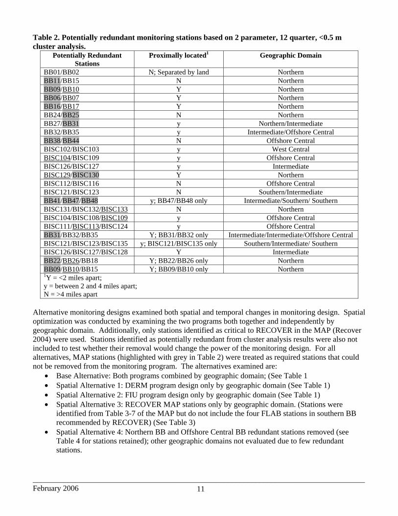
Table 2. Potentially redundant monitoring stations based on 2 parameter, 12 quarter, <0.5 m cluster analysis.

Potentially Redundant Stations

Proximally located1 Geographic Domain

BB01/BB02 N; Separated by land Northern BB11/BB15 N Northern BB09/BB10 Y Northern BB06/BB07 Y Northern BB16/BB17 Y Northern BB24/BB25 N Northern BB27/BB31 y Northern/Intermediate BB32/BB35 y Intermediate/Offshore Central BB38/BB44 N Offshore Central BISC102/BISC103 y West Central BISC104/BISC109 y Offshore Central BISC126/BISC127 y Intermediate BISC129/BISC130 Y Northern BISC112/BISC116 N Offshore Central BISC121/BISC123 N Southern/Intermediate BB41/BB47/BB48 y; BB47/BB48 only Intermediate/Southern/ Southern BISC131/BISC132/BISC133 N Northern BISC104/BISC108/BISC109 y Offshore Central BISC111/BISC113/BISC124 y Offshore Central BB31/BB32/BB35 Y; BB31/BB32 only Intermediate/Intermediate/Offshore Central BISC121/BISC123/BISC135 y; BISC121/BISC135 only Southern/Intermediate/ Southern BISC126/BISC127/BISC128 Y Intermediate BB22/BB26/BB18 Y; BB22/BB26 only Northern BB09/BB10/BB15 Y; BB09/BB10 only Northern 1Y = <2 miles apart; y = between 2 and 4 miles apart; N = >4 miles apart

Alternative monitoring designs examined both spatial and temporal changes in monitoring design. Spatial optimization was conducted by examining the two programs both together and independently by geographic domain. Additionally, only stations identified as critical to RECOVER in the MAP (Recover 2004) were used. Stations identified as potentially redundant from cluster analysis results were also not included to test whether their removal would change the power of the monitoring design. For all alternatives, MAP stations (highlighted with grey in Table 2) were treated as required stations that could not be removed from the monitoring program. The alternatives examined are:

• Base Alternative: Both programs combined by geographic domain; (See Table 1 • Spatial Alternative 1: DERM program design only by geographic domain (See Table 1) • Spatial Alternative 2: FIU program design only by geographic domain (See Table 1) • Spatial Alternative 3: RECOVER MAP stations only by geographic domain. (Stations were

identified from Table 3-7 of the MAP but do not include the four FLAB stations in southern BB recommended by RECOVER) (See Table 3)

• Spatial Alternative 4: Northern BB and Offshore Central BB redundant stations removed (see Table 4 for stations retained); other geographic domains not evaluated due to few redundant stations.

_____________________________________________________________________________________ February 2006 12

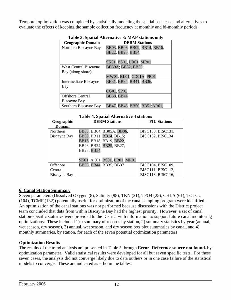
Temporal optimization was completed by statistically modeling the spatial base case and alternatives to evaluate the effects of keeping the sample collection frequency at monthly and bi-monthly periods.

Table 3. Spatial Alternative 3: MAP stations only Geographic Domain DERM Stations

Northern Biscayne Bay BB03, BB06, BB09, BB14, BB16, BB22, BB25, BB54, SK01, BS01, LR01, MR01

West Central Biscayne Bay (along shore)

BB39A; BB52, BB53; MW01, BL01, CD01A, PR01

Intermediate Biscayne Bay

BB31, BB34, BB41, BB36, CG01, SP01


BB38, BB44

Southern Biscayne Bay BB47, BB48, BB50, BB51;AR01,

Table 4. Spatial Alternative 4 stations Geographic

Domain DERM Stations FIU Stations

Northern Biscayne Bay

BB03, BB04, BB05A, BB06, BB09, BB11, BB14, BB15; BB16, BB18, BB19, BB22, BB23, BB24, BB25, BB27, BB28, BB54, SK01, AC01, BS01, LR01, MR01

BISC130, BISC131, BISC132, BISC134


BB38, BB44, BB35, BB37 BISC104, BISC109, BISC111, BISC112, BISC113, BISC116,

6. Canal Station Summary Seven parameters (Dissolved Oxygen (8), Salinity (98), TKN (21), TPO4 (25), CHLA (61), TOTCU (104), TCMF (132)) potentially useful for optimization of the canal sampling program were identified. An optimization of the canal stations was not performed because discussions with the District project team concluded that data from within Biscayne Bay had the highest priority. However, a set of canal station-specific statistics were provided to the District with information to support future canal monitoring optimizations. These included 1) a summary of records by station, 2) summary statistics by year (annual, wet season, dry season), 3) annual, wet season, and dry season box plot summaries by canal, and 4) monthly summaries, by station, for each of the seven potential optimization parameters Optimization Results The results of the trend analysis are presented in Table 5 through Error! Reference source not found. by optimization parameter. Valid statistical results were developed for all but seven specific tests. For these seven cases, the analysis did not converge likely due to data outliers or in one case failure of the statistical models to converge. These are indicated as –rho in the tables.

_____________________________________________________________________________________ February 2006 13

Several broad generalizations are evident across the five domains and five optimization parameters. The base case APC for TPO4 (Table 5) in all domains is at least 100 times lower (range 0.06 and 0.22%) than the 20% target APC (note the period of record analyzed for TPO4 did not include the 1992 and 1993 data as the data from this year appeared to be systematically high relative to the post 1994 data and was removed from the statistical analysis). Salinity had the highest APC with the base case consistently greater than 300% for the Northern and West Central Bay (Table 6). The lowest APC (48%) is associated with the Offshore Biscayne Bay. The other two geographic domains had intermediate values of 88% (Intermediate Biscayne Bay) and 234% (Southern Bay). The APC for dissolved oxygen (DO) (Table 7) and chlorophyll (Table 8) generally fall in the 12 to 15% range for the base case, slightly below the 20% target APC. DO in the West Central Bay and chlorophyll in the Northern Bay are each greater than 20% APC. The APC for TOTN (FIU data only) was typically in the three or lower percent range (Table 9). Regarding the spatial alternatives, the combined data sets generally provide a lower APC than the individual programs, but not always (e.g., salinity in Northern Biscayne Bay). Moreover, the 15 day base sampling scenario generally gave the lowest APC with the monthly and bi-monthly results increasing slightly relative to the base case. The removal of redundant stations in Northern Biscayne Bay substantially decreased the APC for salinity (from 480 to 70). Moreover the individual program and MAP only alternatives provided lower APC, where as changing the frequency of the base case sampling did not alter the base case APC substantially. The APC for the MAP only stations both increased and decreased relative to the full set of DERM stations, although several comparisons showed little change. Overall the analysis suggests that each optimization parameter is behaving independently, and those with the most variability showing the least ability to detect APCs in the slope. Specific observations for each parameter are considered below. TPO4 There is very little difference in the APC among the alternatives examined by geographic domain (Table 5). The largest changes across the alternatives appear in the West Central Bay (0.22 to 0.37% APC), well below the 20 percent level used as a target for change detection, which indicates strong ability to detect a trend in the data. Lower sampling frequencies (monthly and bi-monthly alternatives) increase the APC by only 0.01 to 0.04%. Some spatial alternatives (MAP only Intermediate Biscayne Bay) can double the APC of the base case but the APC never exceeds 0.37% (DERM only West Central Biscayne Bay) for any alternative evaluated. Thus, the sampling programs, either alone or combined or reduced, as in the MAP alternative, have substantial ability to detect small changes in the TPO4 trends. This suggests the programs are very robust relative to this parameter and that the APC is adequate to detect very low target changes in the TPO4. Moreover, reductions in the spatial and temporal monitoring for TPO4 are supported by the analyses, and would not impact the ability to detect trends in the TPO4. Dissolved Oxygen The APC for DO generally falls five percentage points below the 20 percent level used as a target for change detection (Table 6). The higher than 20 percent APC for Western Central Biscayne Bay is ascribed to the high variability in the data and the way stations were selected for inclusion in an alternative. None of the alternatives produced the ability to detect an APC that approaches the 20% target. Interestingly, use of the DERM stations only results in a higher APC than the FIU only alternative. This is likely related to inclusion of the seaward most canal stations which undergo large variability due to variable flow regimes, and a more stable sub region sampled by FIU. Comparison of the MAP Alterative, which removed two canal stations from the DERM alternative, increased the APC, reflecting the high variability in this region of the Bay. To reduce the APC in this region will require more stations and possibly higher frequency sampling. Various combinations of higher frequency sampling at more stations should also be considered. As with TPO4, the magnitude of change that is of concern should be defined.

_____________________________________________________________________________________ February 2006 14

Chlorphyll The lowest base case APC for chlorophyll (7%) was found for the Outer Bay domain; the highest is in the Northern Bay at 17 percent (Table 1). Decreasing sampling frequency of the combined program (base case) adds two to ten points to the APC, with only the Northern Bay reaching APC in the 40 percent for bi-monthly sampling. The spatial alternatives, especially the MAP alternative, results in a doubling of the APC relative to the full set of DERM stations. This may be in part due to removal of redundant stations or to incomplete capture of the spatial variability in the domain by FIU. Total Nitrogen Since the FIU program alone produces data for this parameter, only temporal sampling alternatives could be tested (Table 9). The data show decreasing the sampling interval to bi-monthly from monthly would increase the APC by ~1%, with the lowest APC (4.9 percent) observed in the West Central Bay. The analysis suggests the sampling program is moderately robust and that the agencies should evaluate what APC for this parameter is reasonable for the program. If it is less than the 2-4 percent that can be met presently, higher frequency sampling may be in order. If not, the monitoring program could be reduced to bi-monthly and possibly quarterly without great loss of information. Salinity The largest APC for the base cases were associated with the geographic domains that are subject to the greatest influence of fresh water input (Northern West Central and Southern Bay areas) (Table 6). The ability to detect smaller changes improved in the offshore directions Western Central through the outer Biscayne Bay domains, although none of the geographic regions reached the target 20% APC used in the analysis. Statistical analysis of the DERM and FIU data individually shows large disparity in the APC in the West Central (1,525 percent for DERM compared to FIUs 178 percent), Intermediate Bay (1,050 versus 219 percent), and Southern Bay (514 versus 121 percent). The disparity between the programs is less for the offshore and Northern Bay. The differences relate in part to the stations included in the analysis. The FIU program purposely locates stations outside of channels and away from the direct influence of canals and navigation channels. In contrast, the DERM stations, particularly in the Northern and West Central domains, are specifically chosen to sample the more highly variable regions and include the seaward most canal stations, which can undergo substantial shifts in salinity in response to water flow regulation. In the West Central Bay, the FIU stations, while variable, are in areas where the water has experienced more mixing which homogenizes the salinity signal to some extent. The statistical analysis indicates the sampling programs are relatively poor at detecting changes in salinity, thus the ability to document the response of the system to changes in fresh water flow regimes. Either more sampling more stations or the current stations at higher frequency or both is required to lower the APC. The programs should determine a priori what level of salinity change detection is necessary, and optimize the program around that value. Optimization Recommendations Programmatic

• The responsible agencies should continue efforts to ensure the two programs report comparable data.

• The rationale for the parameters monitored at stations in Biscayne Bay by the two programs should be reassessed and the measurement program brought into alignment. Part of this effort should be to continue to develop and refine conceptual models on how the system works (e.g., how salinity and the nutrient parameters covary) and questions that the monitoring should address.

_____________________________________________________________________________________ February 2006 15

• Better coordination between the monitoring programs (i.e., analytical methods, stations, frequency, depths sampled, and timing of surveys) should be considered as means of providing a more robust data set.

• Consider having both programs include both methods for ammonia analysis. Alternatively, evaluate which is most relevant to the data uses and have the two programs converge on one method.

• Co-located stations may not need to be sampled by both programs. • Consider relocation of several stations within each program to address spatial gaps and address

the known hydrographic gradients within the Bay and better support long-term change detection, especially West Central Biscayne Bay and possibly the Southern Bay.

• Evaluate whether stations located in Southern Biscayne Bay that are routinely monitored under the Florida Bay Monitoring Program (FLAB) should be considered in the BISC monitoring program.

• The specific rationale for each station in the monitoring plan should be revisited from the perspective of spatial sampling redundancy.

• For all parameters except salinity, lower sampling frequency could be considered and likely will not substantially affect the programs’ ability to describe the baseline conditions or detect trends.

_____________________________________________________________________________________ February 2006 16

Table 5. Comparison of Annual Percentage Change detectable with 80% power and p =0.05 for Base and alternative monitoring designs for TPO4. n = the number of periods in year, N = the number of stations in the alternative.

NBD Parameter

Base at 15 day

sampling interval

DERM stations

at 15 day sampling interval

FIU stations


MAP stations

only at 15 day

sampling interval

Base Design at 15 day sampling

interval no redundant

stations

Base Design at monthly sampling interval

Base Design at bi-

monthly sampling interval

Northern

Biscayne Bay 0.06 0.08 0.19 0.16 0.06 0.08 0.10

West Central Biscayne bay 0.22 0.37 0.14 0.18 NA 0.24 0.29

Intermediate Biscayne Bay 0.07 0.12 0.10 0.15 NA 0.09 0.11

Offshore Biscayne

Bay) 0.08 0.07 0.10 0.04 0.08 0.09 0.12

Southern Biscayne Bay 0.07 0.09 0.09 0.08 NA 0.08 0.11

Table 6. Comparison of Annual Percentage Change detectable with 80% power and p =0.05 for Base and alternative monitoring designs for salinity. n = the number of periods in year, N = the number of stations in the alternative.

NBD Parameter

Base at 15 day

sampling interval

DERM stations


FIU stations


MAP stations

only at 15 day

sampling interval



stations


Base Design at bi-


Northern

Biscayne Bay 482 143 39 140 70 519 567

West Central Biscayne bay 329 1,525 178 -rho NA 538 1184

Intermediate Biscayne Bay 118 1048 219 187 NA 144 217

Offshore Biscayne

Bay) 48 126 56 168 49 60 88

Southern Biscayne Bay 234 514 121 707 NA 255 343

_____________________________________________________________________________________ February 2006 17

Table 7. Comparison of Annual Percentage Change detectable with 80% power and p =0.05 for Base and alternative monitoring designs for dissolved oxygen. n = the number of periods in year, N = the number of stations in the alternative.

NBD Parameter

Base at 15 day

sampling interval

DERM stations


FIU stations


MAP stations

only at 15 day

sampling interval



stations


Base Design at bi-


Northern

Biscayne Bay 15 12 -rho 21 16 18 23

West Central Biscayne bay 26 41 30 47 NA 38 57


Offshore Biscayne

Bay) 12 15 16 -rho 12 17 25

Southern Biscayne Bay 12 15 -rho 19 NA 18 26

Table 8. Comparison of Annual Percentage Change detectable with 80% power and p =0.05 for Base and alternative monitoring designs for chlorophyll. n = the number of periods in year, N = the number of stations in the alternative.

NBD Parameter

Base at 15 day

sampling interval

DERM stations


FIU stations


MAP stations

only at 15 day

sampling interval



stations


Base Design at bi-


Northern

Biscayne Bay 25 -rho 32 17 24 30 42

West Central Biscayne bay 17 6.1 15.4 4.1 NA 19 22


Offshore Biscayne

Bay) 7.2 1.6 10 1.6 7.2 8.2 9.8

Southern Biscayne Bay 15 -rho 11 -rho NA 17 23

_____________________________________________________________________________________ February 2006 18

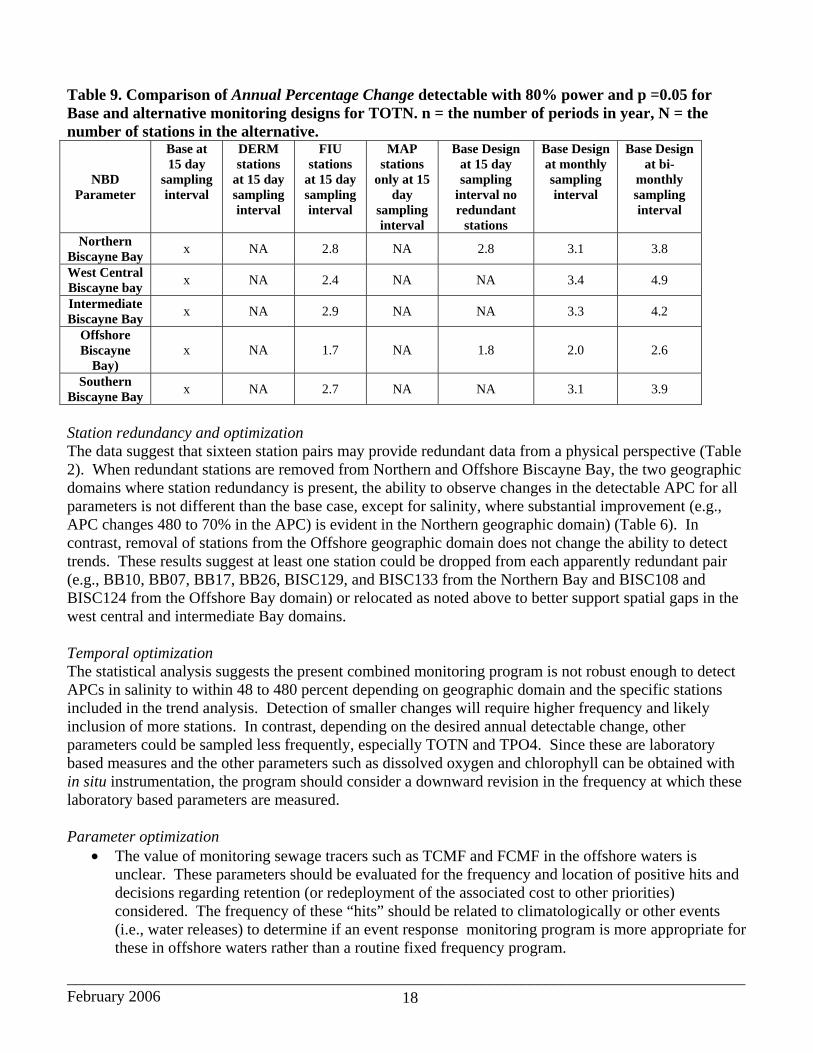
Table 9. Comparison of Annual Percentage Change detectable with 80% power and p =0.05 for Base and alternative monitoring designs for TOTN. n = the number of periods in year, N = the number of stations in the alternative.

NBD Parameter

Base at 15 day

sampling interval

DERM stations


FIU stations


MAP stations

only at 15 day

sampling interval



stations


Base Design at bi-


Northern

Biscayne Bay x NA 2.8 NA 2.8 3.1 3.8

West Central Biscayne bay x NA 2.4 NA NA 3.4 4.9

Intermediate Biscayne Bay x NA 2.9 NA NA 3.3 4.2

Offshore Biscayne

Bay) x NA 1.7 NA 1.8 2.0 2.6

Southern Biscayne Bay x NA 2.7 NA NA 3.1 3.9

Station redundancy and optimization The data suggest that sixteen station pairs may provide redundant data from a physical perspective (Table 2). When redundant stations are removed from Northern and Offshore Biscayne Bay, the two geographic domains where station redundancy is present, the ability to observe changes in the detectable APC for all parameters is not different than the base case, except for salinity, where substantial improvement (e.g., APC changes 480 to 70% in the APC) is evident in the Northern geographic domain) (Table 6). In contrast, removal of stations from the Offshore geographic domain does not change the ability to detect trends. These results suggest at least one station could be dropped from each apparently redundant pair (e.g., BB10, BB07, BB17, BB26, BISC129, and BISC133 from the Northern Bay and BISC108 and BISC124 from the Offshore Bay domain) or relocated as noted above to better support spatial gaps in the west central and intermediate Bay domains. Temporal optimization The statistical analysis suggests the present combined monitoring program is not robust enough to detect APCs in salinity to within 48 to 480 percent depending on geographic domain and the specific stations included in the trend analysis. Detection of smaller changes will require higher frequency and likely inclusion of more stations. In contrast, depending on the desired annual detectable change, other parameters could be sampled less frequently, especially TOTN and TPO4. Since these are laboratory based measures and the other parameters such as dissolved oxygen and chlorophyll can be obtained with in situ instrumentation, the program should consider a downward revision in the frequency at which these laboratory based parameters are measured. Parameter optimization

• The value of monitoring sewage tracers such as TCMF and FCMF in the offshore waters is unclear. These parameters should be evaluated for the frequency and location of positive hits and decisions regarding retention (or redeployment of the associated cost to other priorities) considered. The frequency of these “hits” should be related to climatologically or other events (i.e., water releases) to determine if an event response monitoring program is more appropriate for these in offshore waters rather than a routine fixed frequency program.

_____________________________________________________________________________________ February 2006 19

• The value of measuring color in the offshore ocean waters by DERM is not clear. These measurements are typically associated with fresh and drinking water sources or light penetration.

• The value of quarterly metals monitoring in the ocean influenced region of the bay is unclear. Unless there are clear transport mechanisms that bring contaminated water offshore, one would expect metals to be low and consistent in the offshore waters (e.g. station locations are too far from sources and dilution by seawater is likely too great (typically 100 to 1) to cause water quality violations). The available data appears to be at the MDL of the analytical methods and are well below current water quality criteria. As such, event based monitoring may be a more appropriate approach to metals monitoring. Because measurement of metals in coastal waters requires very specialized contamination control techniques for accuracy, the budget associated with these parameters could be reallocated to higher priority parameters.

• The 2004 MAP (RECOVER 2004) suggests adding silicate, TKN, reactive PO4 (aka OPO4), more metals and chlorophyll sampling to the Biscayne Bay monitoring program and that higher frequency sampling be conducted (the implication is that DERM add these to its program as a result of DERM stations being listed in the MAP as key Biscayne Bay stations). For the marine portion of these monitoring programs, adding TOTN to the DERM program may be a more appropriate than adding TKN to enable the two programs to produce more comparable total nitrogen data. However, the statistical evaluation does not appear to support more TOTN sampling. A more advanced conceptual or numeric water quality model may provide information as to which parameters are most relevant, as well as identification of the necessary sampling frequencies.

• Measurement of photosynthetically active radiation (PAR) for the purpose of calculating attenuation coefficients (K) [DBHydro code 197]) was not evaluated in this optimization. However, this measure in District programs is most often associated with seagrass recovery and trend monitoring. As such, measurement of PAR should be restricted to those areas most likely to have concerns regarding reestablishment or maintenance of seagrass.

• Several parameters measured in these programs are important for understanding ecological processes and the changes in these processes that may occur as water flow to the coast is modified under CERP. As such, these parameters are important for description, documentation, and interpretation of process changes. Retention of these types of measures is the mark of a monitoring program that strives to understand the whys and wherefores of observed changes and ensure conceptual models and monitoring questions are appropriately addressed and modified based on scientific evidence.

Monitoring redesign A gradient approach to monitoring the central Bay with more stations sampled more frequently may increase the ability to detect change especially related to the water management changes planned through the CERP. The monitoring data evaluated here and published findings clearly show substantial gradients in the hydrographic data (salinity and temperature) which influence the nutrients and contaminant concentrations and subsequent ecological responses. Moreover it is clear from the performance measures CERP is suggesting for the southern estuaries that changes in salinity in the bottom waters and nutrients in the surface waters in the very nearshore (within 500 m of shore) are key areas of focus. The ability of the two programs to provide data in these regions is currently limited. Potential modifications include:

o Relocation of the six FIU stations (BISC129 to BISC134) presently sampled in northern Biscayne Bay into the along shore regions of the west central Bay or in southern Biscayne Bay in Card or Barnes Sound

o Retention of the DERM stations in the Northern Bay but consider relocating stations that are

_____________________________________________________________________________________ February 2006 20

providing redundant data but not identified in the MAP (RECOVER 2004) as key stations for RECOVER (See Table 1).

o Relocation of offshore DERM stations BB35, BB37, BB38, and BB44 closer to shore to capture more of the near shore variability associated with C100 canal and fill in spatial gaps; DERM utilize FIU data for its offshore monitoring data needs. FIU should consider adding state required parameters to its program, particularly total NH4.

o Retain the MAP identified stations in the monitoring design to ensure program consistency References

Caccia, V.G. and Boyer, K.N. 2005. Spatial patterning of water quality in Biscayne Bay, Florida as a function of land use and water management. Mar. Poll. Bull. 50:1416-1429.

RECOVER. 2004. CERP Monitoring and Assessment Plan. Restoration Coordination and Verification Program. c/o Jacksonville District, United States Army Corps of Engineers, Jacksonville, Florida, and South Florida Water Management District, West Palm Beach, Florida.

Reckhow KH, Kepford K, and Hicks WW (1993). Methods for the Analysis of Lake Water Quality Trends. EPA 841-R-93-003Rust SW. 2005. Power Analysis Procedure for Trend Detection with Accompanying SAS Software. Battelle Report to South Florida Water Management District, November 2005.

Zhang, J., P.B. Ornter, C.J. Fisher, and L.D. Moore, Jr., 1997. Determination of Ammonia in Estuarine and Coastal Waters by Gas Segmented Continuous Flow Colorimetric Analysis. E. J. Arar, Project Officer. Method 349, Version 1. National Exposure Research Laboratory, Office of Research and Development, U.S. Environmental Protection Agency.

_____________________________________________________________________________________ February 2006

21

Parameters Measured by Grab Samples and In Situ Measurements for Project BISC by DERM; Stations identified as key to RECOVER are highlighted. Station Type DO PHa TEMP SCOND SALIN PARK HARDa TOTCD TOTCU TOTPB TOTZN TSS CHLA COLOR TURBI TKN OPO4 NH4 NOX TPb FCMC TCMC AR01 2 m m m m m m qrt qrt qrt qrt qrt bm bm bm bm bm m m m m m BB03 2 m m m m m m qrt qrt qrt qrt qrt bm bm bm bm m m m m M BB06 2 m m m m m m qrt qrt qrt qrt qrt bm bm bm bm m m m m M BB09 2 m m m m m m qrt qrt qrt qrt qrt bm bm bm bm m m m m M BB14 2 m m m m m m qrt qrt qrt qrt qrt bm bm bm bm m m m m m BB16 2 m m m m m m qrt qrt qrt qrt qrt bm bm bm bm m m m m m BB22 2 m m m m m m qrt qrt qrt qrt qrt bm bm bm bm m m m m m BB25 2 m m m m m m qrt qrt qrt qrt qrt bm bm bm bm m m m m m BB31 2 m m m m m m qrt qrt qrt qrt qrt bm bm bm bm m m m m m BB34 2 m m m m m m qrt qrt qrt qrt qrt bm bm bm bm m m m m m BB36 2 m m m m m m qrt qrt qrt qrt qrt bm bm bm bm m m m m m BB38 2 m m m m m m qrt qrt qrt qrt qrt bm bm bm bm m m m m m BB39A 2 m m m m m m qrt qrt qrt qrt qrt bm bm bm bm m m m m m BB41 2 m m m m m m qrt qrt qrt qrt qrt bm bm bm bm m m m m m BB44 2 m m m m m m qrt qrt qrt qrt qrt bm bm bm bm m m m m m BB47 2 m m m m m m qrt qrt qrt qrt qrt bm bm bm bm m m m m m BB48 2 m m m m m m qrt qrt qrt qrt qrt bm bm bm bm m m m m m BB51 2 m m m m m m qrt qrt qrt qrt qrt bm bm bm bm m m m m m BB52 2 m m m m m m qrt qrt qrt qrt qrt bm bm bm bm m m m m m BB53 2 m m m m m m qrt qrt qrt qrt qrt bm bm bm bm m m m m m BB54 2 m m m m m m qrt qrt qrt qrt qrt bm bm bm bm m m m m m BL01 2 m m m m m m qrt qrt qrt qrt qrt bm bm bm bm m m m m m BS01 2 m m m m m m qrt qrt qrt qrt qrt qrt bm bm bm bm bm m m m m m BS04 2 m m m m m m qrt qrt qrt qrt qrt qrt bm bm bm bm bm m m m m m CD01A 2 m m m m m m qrt qrt qrt qrt qrt bm bm bm bm m m m m m CD02 2 m m m m m m qrt qrt qrt qrt qrt qrt bm bm bm bm bm m m m m m CG01 2 m m m m m m qrt qrt qrt qrt qrt bm bm bm bm m m m m m CG07 2 m m m m m m qrt qrt qrt qrt qrt qrt bm bm bm bm bm m m m m m LR01 2 m m m m m m qrt qrt qrt qrt qrt bm bm bm bm m m m m m LR06 2 m m m m m m qrt qrt qrt qrt qrt qrt bm bm bm bm bm m m m m m MI02 2 m m m m m m qrt qrt qrt qrt qrt qrt bm bm bm bm bm m m m m m MR01 2 m m m m m m qrt qrt qrt qrt qrt bm bm bm bm m m m m m MR08 2 m m m m m m qrt qrt qrt qrt qrt qrt bm bm bm bm bm m m m m m MW01 2 m m m m m m qrt qrt qrt qrt qrt bm bm bm bm m m m m m MW04 2 m m m m m m qrt qrt qrt qrt qrt qrt bm bm bm bm bm m m m m m MW13 2 m m m m m m qrt qrt qrt qrt qrt qrt bm bm bm bm bm m m m m m PR03 2 m m m m m m qrt qrt qrt qrt qrt qrt bm bm bm bm bm m m m m m SK01 2 m m m m m m qrt qrt qrt qrt qrt bm bm bm bm m m m m m SK02 2 m m m m m m qrt qrt qrt qrt qrt qrt bm bm bm bm bm m m m m m SP01 2 m m m m m m qrt qrt qrt qrt qrt bm bm bm bm m m m m m TM03 2 m m m m m m qrt qrt qrt qrt qrt qrt bm bm bm bm bm m m m m m TM08 2 m m m m m m qrt qrt qrt qrt qrt qrt bm bm bm bm bm m m m m m AC01 3 m m m m m m qrt qrt qrt qrt qrt bm bm bm bm m m m m m AC02 3 m m m m m m qrt qrt qrt qrt qrt bm bm bm bm m m m m m AC03 3 m m m m m m qrt qrt qrt qrt qrt qrt bm bm bm bm bm m m m m m AR03 3 m m m m m m qrt qrt qrt qrt qrt qrt bm bm bm bm bm m m m m m BB01 3 m m m m m m qrt qrt qrt qrt qrt bm bm bm bm m m m m m BB02 3 m m m m m m qrt qrt qrt qrt qrt bm bm bm bm m m m m m BB04 3 m m m m m m qrt qrt qrt qrt qrt bm bm bm bm m m m m m BB05A 3 m m m m m m qrt qrt qrt qrt qrt bm bm bm bm m m m m m BB07 3 m m m m m m qrt qrt qrt qrt qrt bm bm bm bm m m m m m BB10 3 m m m m m m qrt qrt qrt qrt qrt bm bm bm bm m m m m m BB11 3 m m m m m m Qrt qrt qrt qrt qrt bm bm bm bm m m m m m

_____________________________________________________________________________________ February 2006

22

Station Type DO PHa TEMP SCOND SALIN PARK HARDa TOTCD TOTCU TOTPB TOTZN TSS CHLA COLOR TURBI TKN OPO4 NH4 NOX TPb FCMC TCMC BB15 3 m m m m m m qrt qrt qrt qrt qrt bm bm bm bm m m m m m BB17 3 m m m m m m qrt qrt qrt qrt qrt bm bm bm bm m m m m m BB18 3 m m m m m m qrt qrt qrt qrt qrt bm bm bm bm m m m m m BB19 3 m m m m m m qrt qrt qrt qrt qrt bm bm bm bm m m m m m BB23 3 m m m m m m qrt qrt qrt qrt qrt bm bm bm bm m m m m m BB24 3 m m m m m m qrt qrt qrt qrt qrt bm bm bm bm m m m m m BB26 3 m m m m m m qrt qrt qrt qrt qrt bm bm bm bm m m m m m BB27 3 m m m m m m qrt qrt qrt qrt qrt bm bm bm bm m m m m m BB28 3 m m m m m m qrt qrt qrt qrt qrt bm bm bm bm m m m m m BB29 3 m m m m m m qrt qrt qrt qrt qrt bm bm bm bm m m m m m BB32 3 m m m m m m qrt qrt qrt qrt qrt bm bm bm bm m m m m m BB35 3 m m m m m m qrt qrt qrt qrt qrt bm bm bm bm m m m m m BB37 3 m m m m m m qrt qrt qrt qrt qrt bm bm bm bm m m m m m BB45 3 m m m m m m qrt qrt qrt qrt qrt bm bm bm bm m m m m m BB50 3 m m m m m m qrt qrt qrt qrt qrt bm bm bm bm m m m m m BL02 3 m m m m m m qrt qrt qrt qrt qrt bm bm bm bm bm m m m m m BL03 3 m m m m m m qrt qrt qrt qrt qrt qrt bm bm bm bm bm m m m m m BL12 3 m m m m m m qrt qrt qrt qrt qrt qrt bm bm bm bm bm m m m m m BS10 3 m m m m m m qrt qrt qrt qrt qrt qrt bm bm bm bm bm m m m m m CD05 3 m m m m m m qrt qrt qrt qrt qrt qrt bm bm bm bm bm m m m m m CD09 3 m m m m m m qrt qrt qrt qrt qrt qrt bm bm bm bm bm m m m m m FC03 3 m m m m m m qrt qrt qrt qrt qrt qrt bm bm bm bm bm m m m m m FC15 3 m m m m m m qrt qrt qrt qrt qrt qrt bm bm bm bm bm m m m m m GL02 3 m m m m m m qrt qrt qrt qrt qrt bm bm bm bm m m m m m GL03 3 m m m m m m qrt qrt qrt qrt qrt qrt bm bm bm bm bm m m m m m LR03 3 m m m m m m qrt qrt qrt qrt qrt qrt bm bm bm bm bm m m m m m LR10 3 m m m m m m qrt qrt qrt qrt qrt qrt bm bm bm bm bm m m m m m MI01 3 m m m m m m qrt qrt qrt qrt qrt bm bm bm bm m m m m m MI03 3 m m m m m m qrt qrt qrt qrt qrt qrt bm bm bm bm bm m m m m m MR02 3 m m m m m m qrt qrt qrt qrt qrt bm bm bm bm m m m m m MR03 3 m m m m m m qrt qrt qrt qrt qrt bm bm bm bm m m m m m MR04 3 m m m m m m qrt qrt qrt qrt qrt bm bm bm bm m m m m m MR06 3 m m m m m m qrt qrt qrt qrt qrt bm bm bm bm m m m m m MR07 3 m m m m m m qrt qrt qrt qrt qrt bm bm bm bm m m m m m MR15 3 m m m m m m qrt qrt qrt qrt qrt qrt bm bm bm bm bm m m m m m MW05 3 m m m m m m qrt qrt qrt qrt qrt qrt bm bm bm bm bm m m m m m NO07 3 m m m m m m qrt qrt qrt qrt qrt qrt bm bm bm bm bm m m m m m OL03 3 m m m m m m qrt qrt qrt qrt qrt qrt bm bm bm bm bm m m m m m PR01 3 m m m m m m qrt qrt qrt qrt qrt bm bm bm bm m m m m m PR04A 3 m m m m m m qrt qrt qrt qrt qrt qrt bm bm bm bm bm m m m m m PR08 3 m m m m m m qrt qrt qrt qrt qrt qrt bm bm bm bm bm m m m m m SK09 3 m m m m m m qrt qrt qrt qrt qrt qrt bm bm bm bm bm m m m m m SP04 3 m m m m m m qrt qrt qrt qrt qrt qrt bm bm bm bm bm m m m m m SP08 3 m m m m m m qrt qrt qrt qrt qrt qrt bm bm bm bm bm m m m m m TM02 3 m m m m m m qrt qrt qrt qrt qrt qrt bm bm bm bm bm m m m m m TM05 3 m m m m m m qrt qrt qrt qrt qrt qrt bm bm bm bm bm m m m m m WC02 3 m m m m m m qrt qrt qrt qrt qrt bm bm bm bm m m m m m WC03 3 m m m m m m qrt qrt qrt qrt qrt qrt bm bm bm bm bm m m m m m WC04 3 m m m m m m qrt qrt qrt qrt qrt qrt bm bm bm bm bm m m m m m BB46 m m m m m m qrt qrt qrt qrt qrt bm bm bm bm m m m m m CD01 m m m m m m qrt qrt qrt qrt qrt bm bm bm bm m m m m m LR02 m m m m m m qrt qrt qrt qrt qrt bm bm bm bm m m m m m m = monthly, bm = bi-monthly, qrt = quarterly; a = questionable value as routine parameter in coastal and marine water; b= Databases carry this as TPO4 not TP

_____________________________________________________________________________________ February 2006 23

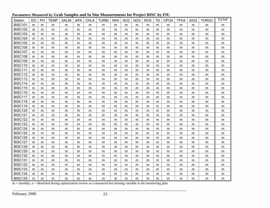
Parameters Measured by Grab Samples and In Situ Measurements for Project BISC by FIU Station DO PH TEMP SALIN APA CHLA TURBI NH4 NO2 NO3 NOX TN OPO4 TPO4 SIO2 TORGC TOTNa BISC101 m m m m m m m m m m m m m m m m m BISC102 m m m m m m m m m m m m m m m m m BISC103 m m m m m m m m m m m m m m m m m BISC104 m m m m m m m m m m m m m m m m m BISC105 m m m m m m m m m m m m m m m m m BISC106 m m m m m m m m m m m m m m m m m BISC107 m m m m m m m m m m m m m m m m m BISC108 m m m m m m m m m m m m m m m m m BISC109 m m m m m m m m m m m m m m m m m BISC110 m m m m m m m m m m m m m m m m m BISC111 m m m m m m m m m m m m m m m m m BISC112 m m m m m m m m m m m m m m m m m BISC113 m m m m m m m m m m m m m m m m m BISC114 m m m m m m m m m m m m m m m m m BISC115 m m m m m m m m m m m m m m m m m BISC116 m m m m m m m m m m m m m m m m m BISC117 m m m m m m m m m m m m m m m m m BISC118 m m m m m m m m m m m m m m m m m BISC119 m m m m m m m m m m m m m m m m m BISC120 m m m m m m m m m m m m m m m m m BISC121 m m m m m m m m m m m m m m m m m BISC122 m m m m m m m m m m m m m m m m m BISC123 m m m m m m m m m m m m m m m m m BISC124 m m m m m m m m m m m m m m m m m BISC125 m m m m m m m m m m m m m m m m m BISC126 m m m m m m m m m m m m m m m m m BISC127 m m m m m m m m m m m m m m m m m BISC128 m m m m m m m m m m m m m m m m m BISC129 m m m m m m m m m m m m m m m m m BISC130 m m m m m m m m m m m m m m m m m BISC131 m m m m m m m m m m m m m m m m m BISC132 m m m m m m m m m m m m m m m m m BISC133 m m m m m m m m m m m m m m m m m BISC134 m m m m m m m m m m m m m m m m m BISC135 m m m m m m m m m m m m m m m m m

m = monthly; a = identified during optimization review as a measured but missing variable in the monitoring plan

_____________________________________________________________________________________ February 2006 24

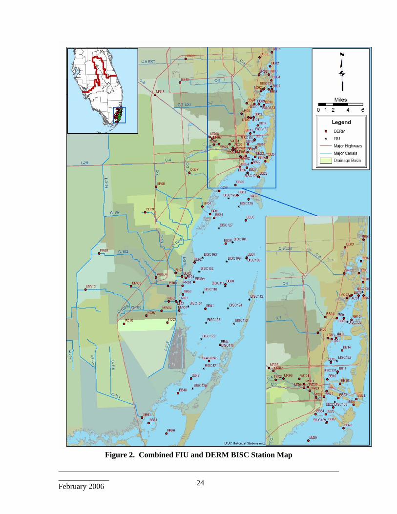
Figure 2. Combined FIU and DERM BISC Station Map

_____________________________________________________________________________________ February 2006 25

Appendix 1: Data uses within the BISC The evaluation of the mandates and monitoring objectives for the two monitoring program deployed in Biscayne Bay identified twelve primary data uses (See BISC Optimization Plan, Battelle 2005). Also identified were statistical analysis procedures and an optimization metric that could be used to assess the effect of optimization options considered. These were modified as the optimization proceeded and resource constraints came into play. 1. Estimate baseline coastal parameter concentrations for stations with common physical

associations (e.g., central region, northern Biscayne Bay, etc.) A. Statistical analysis procedure: 95% confidence interval for the true average

parameter concentration B. Optimization metric: Length or relative length of the 95% confidence interval

2. Estimate baseline parameter concentrations for stations with common physical

associations (i.e., canals, geographic domains in Biscayne bay) A. Statistical analysis procedure: 95% confidence interval for the true average


3. Estimate long-term coastal parameter concentration trends for stations with common

physical associations A. Statistical analysis procedure: 95% confidence interval for the slope of a

regression line describing true average parameter concentration versus time B. Optimization metric: Length or relative length of the 95% confidence

4. Estimate long-term parameter concentration trends for stations with common physical

associations (i.e. canals, Biscayne Bay geographic domains) A. Statistical analysis procedure: 95% confidence interval for the slope of a


5. Detect changes in coastal parameter concentrations that result from climatic cycles,

events, watershed changes A. Statistical analysis procedure: T-test of the hypothesis that the true average

parameter concentration after the event/action is equal to the true average parameter concentration before the event/action

B. Optimization metric: The minimum percentage change (after vs. before) that is detectable with 80% power

6. Detect changes in canal parameter concentrations that result from climatic cycles,

events, watershed changes

_____________________________________________________________________________________ February 2006 26

A. Statistical analysis procedure: T-test of the hypothesis that the true average parameter concentration after the event/action is equal to the true average parameter concentration before the event/action


7. Enable documentation of changes in temporal and spatial trends of known “hotspots”

in the system A. Statistical analysis procedure: Define gradient in terms of the slope of a

regression line describing parameter concentration versus time or location. T-test of hypothesis that the true current slope is equal to the true historical slope.

B. Optimization metric: The minimum percentage change in slope that is detectable with 80% power

8. Enable documentation of changes in water quality resulting from comprehensive

storm water improvement programs. A. Statistical analysis procedure: T-test of the hypothesis that the true average



9. Detect changes resulting in the project area from alterations in freshwater source

strengths and hydrological changes. A. Statistical analysis procedure: T-test of the hypothesis that the true average



10. Estimate baseline parameter concentrations to support development of non-

degradation criteria (e.g., TMDLs) for nutrients and contaminant metals A. Statistical analysis procedure: 95% confidence interval for the true average


11. Estimate trends in parameter concentrations to support assessment of progress toward

the achievement of non-degradation criteria (e.g., TMDLs) for nutrients and contaminant metals A. Statistical analysis procedure: 95% confidence interval for the slope of a


_____________________________________________________________________________________ February 2006 27

Appendix 2: Inter-laboratory Comparison For the marine portion of the study (Biscayne Bay), data from two laboratories (DERM and FIU) were available and required comparison to determine which parameters are comparable and what data and stations should be used for the optimization phase. Only one laboratory (DERM) performs the measurements on the fresh water samples (canals located throughout the project domain). To conduct the optimization process, a series of questions were asked. Those related to the laboratory inter-comparison are addressed in the following section.

Inter laboratory Comparison parameters 1. Are there co-located stations that can be used for inter-laboratory data

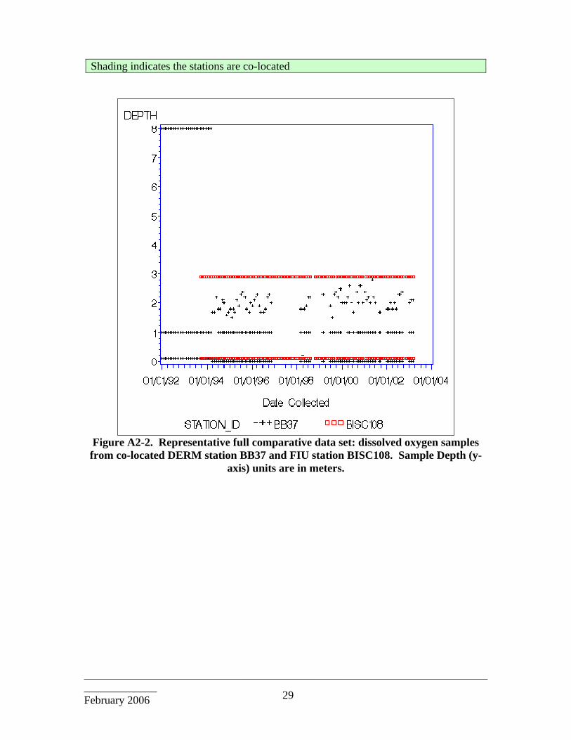
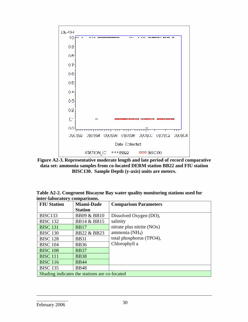
comparisons? Examination of the GIS map of the stations identified 13 congruent station pairs for potential comparison (Figure A2-1) of which four (Table A2-1) are co-located (overlay on the map). The others were within in a few hundred meters of each other. The database was examined for these thirteen stations using dissolved oxygen to determine the temporal overlap in data records. The lengths of the data records were characterized as full, moderate, or short and as early or late in the period of record by plotting the date of sample collection versus the depth of the sample collection. Representative examples of long and moderate length records are shown in Figure (BB37 vs BISC108) and Figure (BB22 vs BISC130). Several stations listed in the project summary were found to have early, short periods of record (i.e. BISC105, 106, 107, 114, 115, 117, 118, 119, 120, and 125). BISC stations 126, 127, 128, 129, 130, 131, 132, 133, 134, and 135 had moderate length data records obtained since 1996. The DERM data (DERM stations are designated with BB; FIU stations with BISC) from Biscayne Bay has generally covered the entire period since 1993. Only those stations characterized as having a moderate data set late in the period of record, or a full data set for the entire period of record were retained for the inter-laboratory comparison (Table A2-2).

_____________________________________________________________________________________ February 2006 28

Figure A2-1. GIS layer of current project sampling positions. Table A2-1. Congruent sample locations for parameter inter-comparison. The length of the data records were characterized as full (F), moderate (M), or short (S) and as early (E) or late (L) in the period of record.

FIU Station Miami-Dade Station

Preliminary Comparison Parameters

BISC134 (M,L) BB05A (S,L) BISC133 (M,L) BB09 & BB10 (F) BISC132 (M,L) BB14 & BB15 (F) BISC131 (M,L) BB17 (F) BISC130 (M,L) BB22 & BB23 (F) BISC128 (M,L) BB31 (F) BISC104 (F) BB36 (F) BISC108 (F) BB37 (F) BISC111 (F) BB38 (F) BISC116 (F) BB44 (F)

Dissolved Oxygen (DO), salinity, nitrate plus nitrite (e.g., NOx), ammonia (NH4), total nitrogen measures (i.e., TKN vs TOTN), total phosphorus (i.e. TP vs TPO4), and chlorophyll a.

BISC121 (F) BB46 (M,E) BISC135 (M,L) BB48 (F) BISC125 (S,E) BB41 (F)

_____________________________________________________________________________________ February 2006 29

Shading indicates the stations are co-located

Figure A2-2. Representative full comparative data set: dissolved oxygen samples from co-located DERM station BB37 and FIU station BISC108. Sample Depth (y-

axis) units are in meters.

_____________________________________________________________________________________ February 2006 30

Figure A2-3. Representative moderate length and late period of record comparative

data set: ammonia samples from co-located DERM station BB22 and FIU station BISC130. Sample Depth (y-axis) units are meters.

Table A2-2. Congruent Biscayne Bay water quality monitoring stations used for inter-laboratory comparisons.

FIU Station Miami-Dade Station

Comparison Parameters

BISC133 BB09 & BB10 BISC 132 BB14 & BB15 BISC 131 BB17 BISC 130 BB22 & BB23 BISC 128 BB31 BISC 104 BB36 BISC 108 BB37 BISC 111 BB38 BISC 116 BB44

Dissolved Oxygen (DO), salinity nitrate plus nitrite (NOx) ammonia (NH4) total phosphorus (TPO4), Chlorophyll a

BISC 135 BB48 Shading indicates the stations are co-located

_____________________________________________________________________________________ February 2006 31

2. What parameters can be inter-compared? Table compares the sample collection frequency for the two water types (canals and ocean) sampled under BISC based on the monitoring plan and project summary. Table A2-3 lists set of parameters initially identified for inter-comparison based on the sampling frequency reported by each monitoring program. These data were considered most the likely candidates for data similarity (e.g., TKN versus Total Nitrogen [TOTN]). The parameters listed in Table are for Biscayne Bay (ocean) only, as FIU conducts monitoring exclusively in the Bay and not in the canals. Thus, no inter-laboratory comparison was possible for the fresh water data.

The parameters in Table A2-3 were evaluated as under question 1 (i.e., time versus depth of samples) to develop the final parameter comparison set. This approach identified that TKN was not included in the DERM data for the Biscayne Bay stations, although listed in the BISC project monitoring plans and project summary. Thus, the planned inter-comparison for total nitrogen measures (TKN and TOTN) could not be made and this parameter set was eliminated from the effort. It was also found that there is no TP (Particulate Phosphate - Code 101) in the database developed for this BISC optimization. The depth versus time plots (Figure A2-4) revealed that TPO4 is measured under both programs. Therefore, TPO4 was included in the inter-laboratory comparison. Because different depths are sampled in the Bay by these programs, the data were stratified into surface water (<0.5 m depth) and subsurface samples for the inter-laboratory comparison. Exact matches in sampling depths were not available. The FIU program consistently reported data from the surface (<0.5m) and 3 meters, while the DERM data varies across several depths depending on the station (see for example Figure A2-2). Therefore, comparison data were classified and combined as follows: data from samples collected near the surface (<0.5m depth) within a single 24 hour period were considered “surface” data; data from samples collected within a depth range of 3±0.9 m within the same sampling day were considered “depth” data. This resulted in four data sets: surface and depth from FIU program and surface and depth data from the DERM program. These data were characterized as described under Question 3 below. Only those parameters that had data from each data set could be compared: These included: dissolved oxygen, salinity, NOx, NH4, orthophosphate, total phosphate, and Chlorophyll a. Turbidity was not compared as water clarity in the bay is high and this parameter was not selected as one of the parameters to use for optimization.

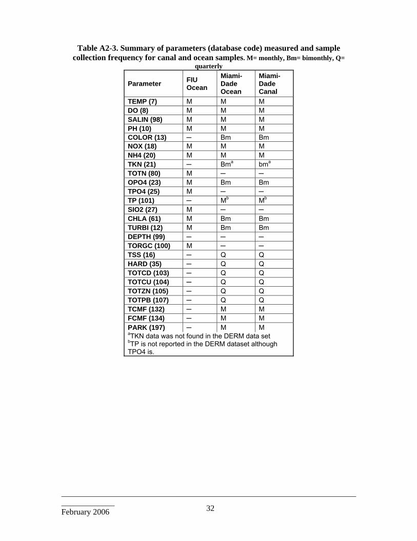
_____________________________________________________________________________________ February 2006 32

Table A2-3. Summary of parameters (database code) measured and sample collection frequency for canal and ocean samples. M= monthly, Bm= bimonthly, Q=

quarterly

Parameter FIU Ocean

Miami-Dade Ocean

Miami-Dade Canal

TEMP (7) M M M DO (8) M M M SALIN (98) M M M PH (10) M M M COLOR (13) ─ Bm Bm NOX (18) M M M NH4 (20) M M M TKN (21) ─ Bma bma TOTN (80) M ─ ─ OPO4 (23) M Bm Bm TPO4 (25) M ─ ─ TP (101) ─ Mb Mb SIO2 (27) M ─ ─ CHLA (61) M Bm Bm TURBI (12) M Bm Bm DEPTH (99) ─ ─ ─ TORGC (100) M ─ ─ TSS (16) ─ Q Q HARD (35) ─ Q Q TOTCD (103) ─ Q Q TOTCU (104) ─ Q Q TOTZN (105) ─ Q Q TOTPB (107) ─ Q Q TCMF (132) ─ M M FCMF (134) ─ M M PARK (197) ─ M M aTKN data was not found in the DERM data set bTP is not reported in the DERM dataset although TPO4 is.

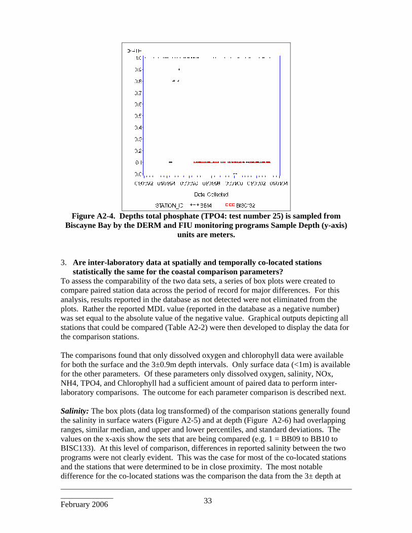
_____________________________________________________________________________________ February 2006 33

Figure A2-4. Depths total phosphate (TPO4: test number 25) is sampled from

Biscayne Bay by the DERM and FIU monitoring programs Sample Depth (y-axis) units are meters.

3. Are inter-laboratory data at spatially and temporally co-located stations

statistically the same for the coastal comparison parameters? To assess the comparability of the two data sets, a series of box plots were created to compare paired station data across the period of record for major differences. For this analysis, results reported in the database as not detected were not eliminated from the plots. Rather the reported MDL value (reported in the database as a negative number) was set equal to the absolute value of the negative value. Graphical outputs depicting all stations that could be compared (Table A2-2) were then developed to display the data for the comparison stations. The comparisons found that only dissolved oxygen and chlorophyll data were available for both the surface and the 3±0.9m depth intervals. Only surface data (<1m) is available for the other parameters. Of these parameters only dissolved oxygen, salinity, NOx, NH4, TPO4, and Chlorophyll had a sufficient amount of paired data to perform inter-laboratory comparisons. The outcome for each parameter comparison is described next. Salinity: The box plots (data log transformed) of the comparison stations generally found the salinity in surface waters (Figure A2-5) and at depth (Figure A2-6) had overlapping ranges, similar median, and upper and lower percentiles, and standard deviations. The values on the x-axis show the sets that are being compared (e.g. 1 = BB09 to BB10 to BISC133). At this level of comparison, differences in reported salinity between the two programs were not clearly evident. This was the case for most of the co-located stations and the stations that were determined to be in close proximity. The most notable difference for the co-located stations was the comparison the data from the 3± depth at

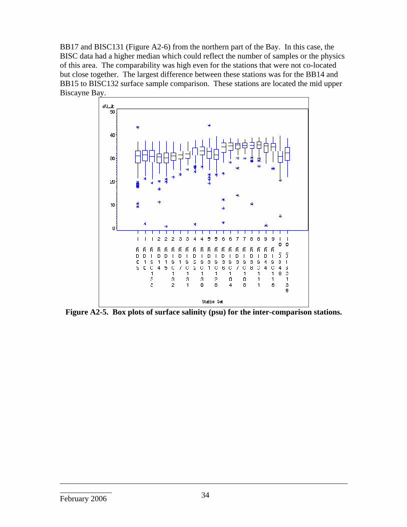
_____________________________________________________________________________________ February 2006 34

BB17 and BISC131 (Figure A2-6) from the northern part of the Bay. In this case, the BISC data had a higher median which could reflect the number of samples or the physics of this area. The comparability was high even for the stations that were not co-located but close together. The largest difference between these stations was for the BB14 and BB15 to BISC132 surface sample comparison. These stations are located the mid upper Biscayne Bay.

Figure A2-5. Box plots of surface salinity (psu) for the inter-comparison stations.

_____________________________________________________________________________________ February 2006 35

Figure A2-6. Box plots of ±3m salinity (psu) for the inter-comparison stations.

Dissolved Oxygen (DO): The paired station box plots comparison shows the DO levels in surface waters and at depth had overlapping ranges, similar median, and upper and lower percentiles, and standard deviations (See Figure A2-7 and Figure A2-8). The BB14 and BB15 to BISC132 surface and bottom waters had the most obvious differences. Thus, there were no clear differences at this level of comparison between the two monitoring programs. This was the case for both the four co-located stations and the stations that were determined to be in close proximity. The small differences noted between the co-located stations were in part due to unequal sample size (n); the differences in the close proximity stations could be due to sample collection timing (offsets in the time of day) as well as the analytical methods, and the depth of samples obtained. Thus this approach did not fully resolve whether the data sets can be compared but suggested the two programs were achieving similar results over the period of record.

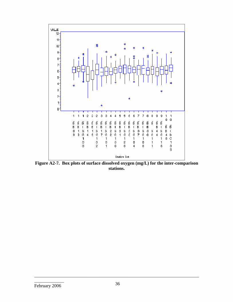
_____________________________________________________________________________________ February 2006 36

Figure A2-7. Box plots of surface dissolved oxygen (mg/L) for the inter-comparison

stations.

_____________________________________________________________________________________ February 2006 37

Figure A2-8. Box plots of ±3m dissolved oxygen (mg/L) for the inter-comparison stations.

Nitrate plus nitrite (NOx): Comparison data for NOx was only available from the surface depth. The FIU data was evaluated to see if the sum of the NO2 and NO3 equaled the reported NOx. For 93 percent of the data, NOx=NO2+NO3 (18% exactly equal, 75% agree to 9th decimal place). For the other 7% of the samples, the difference between NO2+NO3 and NOx ranges from 0.00003 to .0021 mg/L, with sample showing a larger difference of 0.010 mg/L. Some differences may be due to MDL issues or to rounding during the summing. It was determined to focus on the NOx only for the inter-laboratory comparison and optimization effort. The box plots show that while the data from the two programs had overlapping ranges, the median values were not precisely the same, had differences in the upper and lower percentiles, and in the magnitude of the standard deviations (Figure A2-9). This is in part due to differences on the number of data points available for the comparisons. Typically n>100 for FIU and <10 for the DERM data set.

_____________________________________________________________________________________ February 2006 38

Figure A2-9. Box plots of NOx (mg/L) for the inter-comparison stations - surface water.

Ammonia (NH4): Comparison data for NH4 was only available from the surface depth. The box plots show the data from the two programs were very different with no overlap at any of the comparison stations for the period of record (Figure A2-10). Discussions with FIU and DERM project leaders (Joe Boyer, FIU; Steve Blair DERM, October 10, 2005) determined the difference is due to the methods used to make the measurement. DERM uses a total ammonia method (dissolved plus particle bound) that determines ammonia in unfiltered, acidified samples. In contrast FIU uses a filtered but unacidified sample which provides an estimate of the dissolved ammonia.

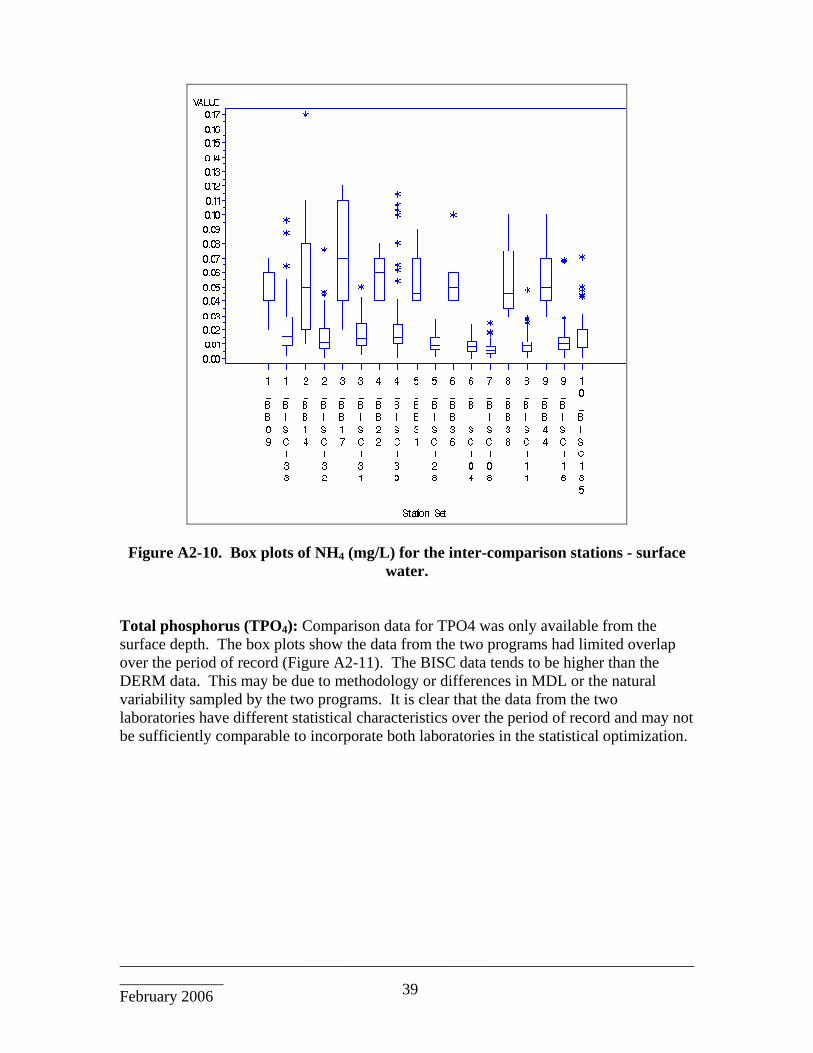
_____________________________________________________________________________________ February 2006 39

Figure A2-10. Box plots of NH4 (mg/L) for the inter-comparison stations - surface water.

Total phosphorus (TPO4): Comparison data for TPO4 was only available from the surface depth. The box plots show the data from the two programs had limited overlap over the period of record (Figure A2-11). The BISC data tends to be higher than the DERM data. This may be due to methodology or differences in MDL or the natural variability sampled by the two programs. It is clear that the data from the two laboratories have different statistical characteristics over the period of record and may not be sufficiently comparable to incorporate both laboratories in the statistical optimization.

_____________________________________________________________________________________ February 2006 40

Figure A2-11. Box plots of TPO4 (mg/L) for the inter-comparison stations - surface

water. Chlorophyll a: The only chlorophyll data available for comparison was from the surface and was limited to five sets of station pairs (BB09/BISC133, BB14/BISC132, BB17/BISC131, and BB38/BISC111) due to limited station data from the DERM program. The box plots for the set of comparison stations suggest the chlorophyll levels in the surface waters of the paired stations were similar with overlapping ranges, similar median, and upper and lower percentiles, and standard deviations (Figure A2-12). The reported chlorophyll levels generally low (<2mg/L) but ranged up to 10mg/L on occasion. At this level of comparison, differences between the two programs were not clearly evident.

_____________________________________________________________________________________ February 2006 41

Figure A2-12. Box plots of chlorophyll a (mg/L) for the inter-comparison stations -

surface water. 4. Do the inter-comparison parameters correlate sufficiently to enable application

of adjustment factors to enable use of the all data for optimization? To address the point by point comparability of the data (data and time, depth, location), paired data (collected within 24 hours and at the similar depths) for all stations in Biscayne Bay were graphed using scatter plots to ascertain the strength of the correlation and whether their was bias between the two measurement programs. The expectation was that the data would be a linear function with a slope of 1:1 if the data sets are fully comparable. Surface and depth samples were included in the plots, although identified separately via symbols. No comparisons were possible for NOx, NH4, and TPO4 due to the small number of “co-collected” samples. Co-located station data was not found for TPO4 as the two programs collect data on different dates and depths. There was some data to compare for the other parameters. For these parameters the number of points that could be compared represented 1-5 percent of the data collected (e.g., only 1-5% of the time did FIU and DERM collect data on the same date and at the same depth). Investigation of the sample collection timing found DERM and FIU sampling dates were usually separated by days, often weeks. Salinity and dissolved oxygen were the only parameters with sufficient data points between the two programs to conduct statistical calculations. While not included in the inter-laboratory comparison data evaluation, temperature data was evaluated

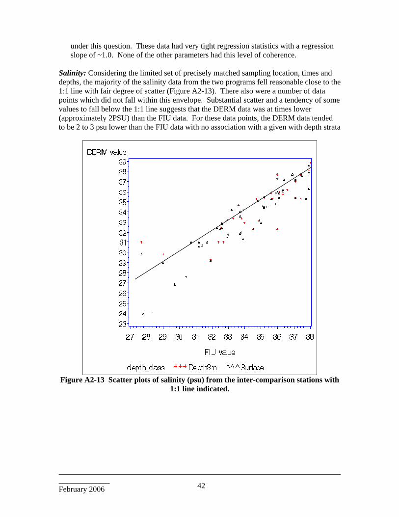
_____________________________________________________________________________________ February 2006 42

under this question. These data had very tight regression statistics with a regression slope of ~1.0. None of the other parameters had this level of coherence.

Salinity: Considering the limited set of precisely matched sampling location, times and depths, the majority of the salinity data from the two programs fell reasonable close to the 1:1 line with fair degree of scatter (Figure A2-13). There also were a number of data points which did not fall within this envelope. Substantial scatter and a tendency of some values to fall below the 1:1 line suggests that the DERM data was at times lower (approximately 2PSU) than the FIU data. For these data points, the DERM data tended to be 2 to 3 psu lower than the FIU data with no association with a given with depth strata

Figure A2-13 Scatter plots of salinity (psu) from the inter-comparison stations with

1:1 line indicated.

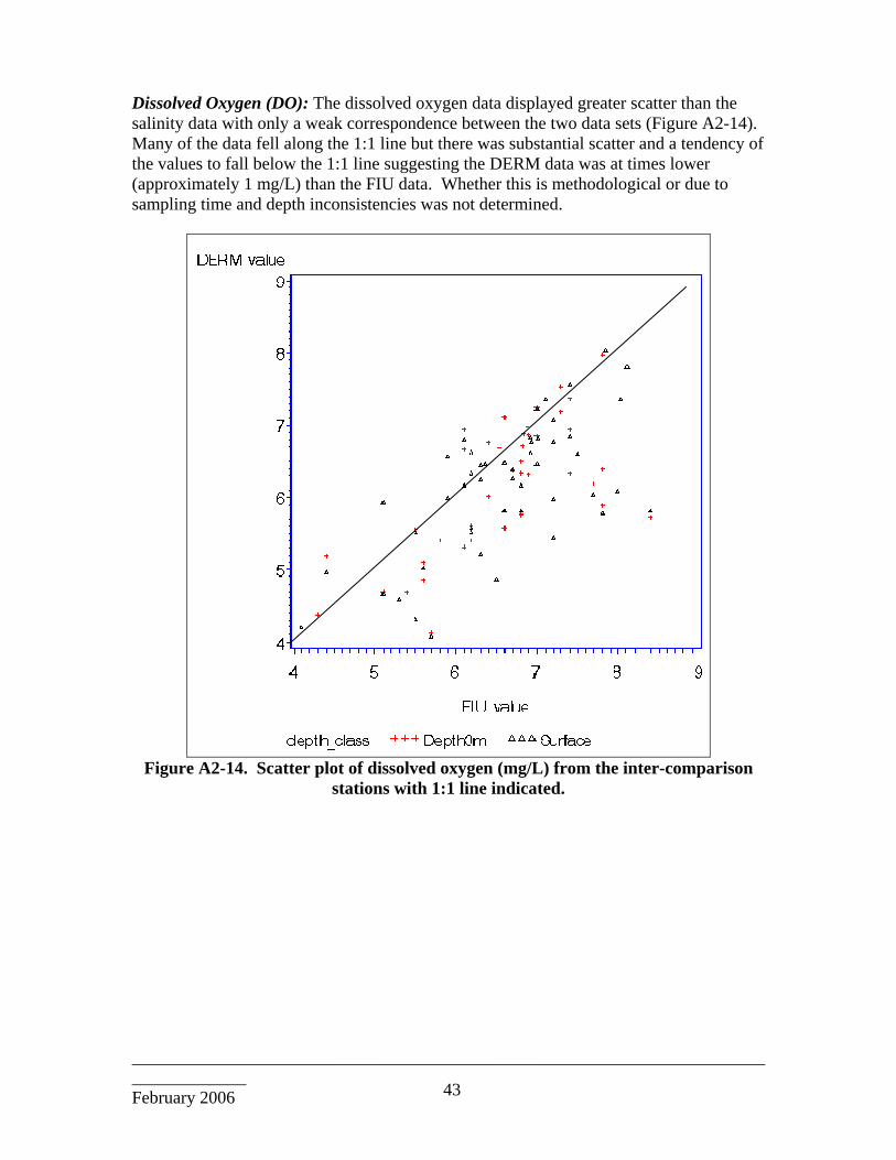
_____________________________________________________________________________________ February 2006 43

Dissolved Oxygen (DO): The dissolved oxygen data displayed greater scatter than the salinity data with only a weak correspondence between the two data sets (Figure A2-14). Many of the data fell along the 1:1 line but there was substantial scatter and a tendency of the values to fall below the 1:1 line suggesting the DERM data was at times lower (approximately 1 mg/L) than the FIU data. Whether this is methodological or due to sampling time and depth inconsistencies was not determined.

Figure A2-14. Scatter plot of dissolved oxygen (mg/L) from the inter-comparison

stations with 1:1 line indicated.

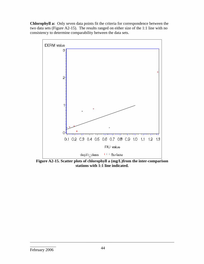
_____________________________________________________________________________________ February 2006 44

Chlorophyll a: Only seven data points fit the criteria for correspondence between the two data sets (Figure A2-15). The results ranged on either size of the 1:1 line with no consistency to determine comparability between the data sets.

Figure A2-15. Scatter plots of chlorophyll a (mg/L)from the inter-comparison

stations with 1:1 line indicated.

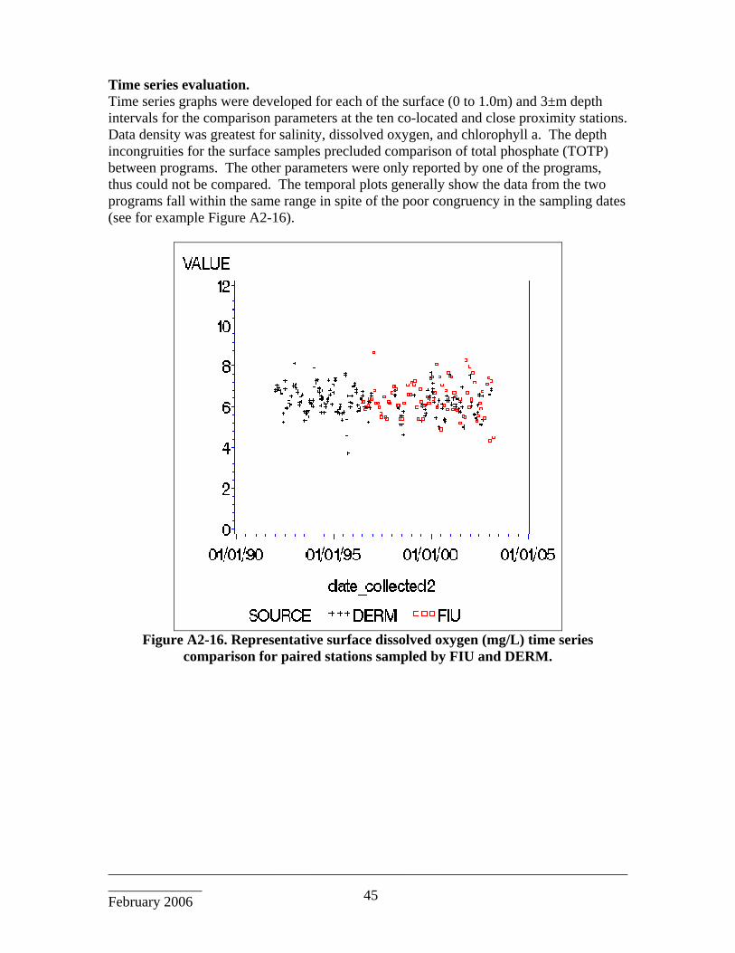
_____________________________________________________________________________________ February 2006 45

Time series evaluation. Time series graphs were developed for each of the surface (0 to 1.0m) and 3±m depth intervals for the comparison parameters at the ten co-located and close proximity stations. Data density was greatest for salinity, dissolved oxygen, and chlorophyll a. The depth incongruities for the surface samples precluded comparison of total phosphate (TOTP) between programs. The other parameters were only reported by one of the programs, thus could not be compared. The temporal plots generally show the data from the two programs fall within the same range in spite of the poor congruency in the sampling dates (see for example Figure A2-16).

Figure A2-16. Representative surface dissolved oxygen (mg/L) time series

comparison for paired stations sampled by FIU and DERM.

_____________________________________________________________________________________ February 2006 46

Appendix 3: Cluster analysis based on 12 time intervals, two parameters, and <0.5 m data. This analysis covered 46 time periods (quarterly averages, from Winter 1992 through Spring 2003) using salinity and temperature from depths less than 0.5m as the primary environmental parameters. This record was reduced to the 12 time periods which yield the most data for the most number of stations: Spring 2000 through winter 2003. The resulting 24 variables were used in cluster analysis (2 parameters times 12 time periods). Of the original 77 stations in the bay, 11 stations were eliminated due to missing data, leaving 66 for the cluster analysis. The eleven eliminated stations were BB46, BISC105, BISC106, BISC107, BISC114, BISC115, BISC117 through BISC120, BISC125. The resulting dendogram is shown in Figure A3-1. As observed in prior clustering analyses, the stations from the two programs form the two major clusters. Three major subgroups were apparent in the DERM data while the FIU data tended to fall into one major group with two major subgroups. The 15 cluster level (Table A3-1) explained 81 percent of the variation. The reanalysis did result in several stations changing their relative association and groupings from previous clustering analyses but did clarify the general geographic associations. The FIU data separated into four major subgroups. These groupings were geographically similar to the four clusters reported by Caccia and Boyer (in press 2005). The DERM data separated into 11 groups with six groups having stations in northern Biscayne Bay. Within the DERM data there are three single station groups (Station BB04 (Group 13), BB11 (Group 14), and BB53 (Group 15) and one group (7) consisting of two noncontiguous regions There is substantial geographic consistency among several of the clusters at the 15 group level. For example, Group 5 (BB) and Group 1 (BISC) are in a geographically similar location in outer central Biscayne Bay. Likewise, Group 11 (BB) and Group 10 (BISC) (in west central Biscayne Bay), and part of Group 6 (BISC) and several DERM derived data groups (Group 2, and Group 4, and Group 14) in northern Biscayne Bay geographically over lay. The geographic distribution of the clusters can be characterized into five general areas: the Southern Biscayne Bay (Manatee Bay and Barnes Sound), Northern Biscayne Bay (Bear Cut to the Oleta River), West Central Biscayne Bay (along shore), Intermediate Central Biscayne Bay (an area extending from north to south through out the central and south central Biscayne Bay, and Offshore Central Biscayne Bay. The Northern Biscayne Bay could be further subdivided based on the DERM data. The Barnes Sound area tends to group more closely with the Intermediate Central Biscayne Bay stations than with the Card sound data.

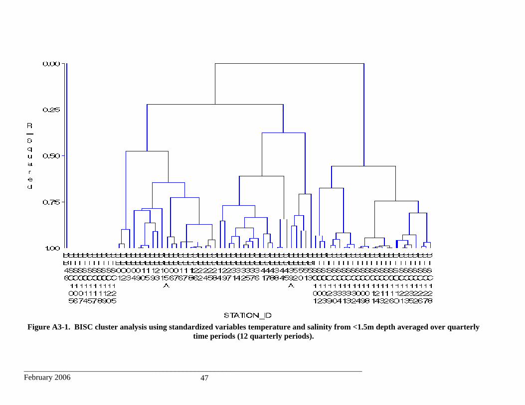
_____________________________________________________________________________________ February 2006 47

Figure A3-1. BISC cluster analysis using standardized variables temperature and salinity from <1.5m depth averaged over quarterly

time periods (12 quarterly periods).

_____________________________________________________________________________________ February 2006 48

Table A3-1. Fifteen-cluster grouping 12 time periods, two parameters, <0.5m – 81% of variation explained.

Cluster# Station

1 BISC104, BISC108, BISC109, BISC111, BISC112, BISC113, BISC116, BISC124

2 BB09, BB10, BB15, BB19, BB23

3 BISC110, BISC121, BISC122, BISC123, BISC126, BISC127, BISC128, BISC135

4 BB16, BB17, BB18, BB22, BB24, BB25, BB26, BB28 5 BB38, BB44, BB45 6 BISC129, BISC130, BISC131, BISC132, BISC133, BISC134 7 BB27, BB31, BB32, BB34, BB35, BB36, BB37, BB41, BB47, BB48 8 BB05A, BB06, BB07 9 BB01, BB02, BB03 10 BISC101, BISC102, BISC103 11 BB39A, BB50, BB51, BB52 12 BB14, BB29 13 BB04 14 BB11 15 BB53

Documents

Biscayne Bay Water Quality Monitoring Networka definition of “hot spots” be developed to guide future optimal monitoring program designs for these regions. 2. Laboratory Inter-Comparison