Embed Size (px)
Citation preview
ISSN: 2394-7772International Journal of
Biomathematics and Systems BiologyOfficial Journal of Biomathematical Society of India
Volume 1, No. 2, Year 2015
A two-prey – diseased predator ecosystem ⋆
Barbara Bonafe, Alice Conchin Gubernati, Giulia Ricci, Ezio Venturino
Dipartimento di Matematica “Giuseppe Peano”, Universita di Torino,
via Carlo Alberto 10, 10123 Torino, Italy
Abstract. In this paper we consider a disease-affected specialist predator that feeds on two re-
sources. While the ecosystem is never wiped out, interestingly, just one prey cannot thrive in it.
Transcritical bifurcations relate the simplest equilibria. Some sufficient conditions for the fea-
sibility of the coexistence equilibrium are derived. In the particular case of the disease being
unrecoverable, some additional healthy-predator-free equilibria are discovered, in which either
one or both prey thrive, together with the infected predators.
Key words: Ecoepidemiology, predator-prey, transmissible disease, two resources, stability.
1 Introduction
Ecoepidemic models investigate the relationships between populations in which diseases play a substantial role, one first paper in
this domain being [18]. An account for the developments of this research field is contained in [29] and the more recent [34]. In
ecoepidemiology, which joins demographic models with epidemic ones, [19, 20, 24, 14, 16, 26], disease can be considered a way
of controlling one, or both, interacting populations, [2], especially if one of them is considered a pest, [4, 1, 30, 27], or when one
population is not really affected by a disease, but may cause harm to the other one which is considered a resource, [10, 11]. Many
models have been formulated in the course of the years. An attempt for a comparative study has been performed in [2]. However,
not just predator-prey ecosystems have been investigated, see for instance [31] for a case involving competing populations. Further,
recently, systems have been investigated leading to more complicated behaviors, [3]. To this end, we also cite some attempts at looking
at food webs, [5, 6, 7, 13]. Note however that in the literature also a kind of symmetric case has been considered, in which two diseases
affect the ecosystem, [12, 25].
We consider here a predator-prey ecoepidemic model in which the predator is affected by a disease and can feed on two different
types of prey. In the absence of either one of them, the model reduces to well-known models in the literature, see e.g. [33, 9].
One example of such a situation in real life is described for instance as follows. Red foxes, (Vulpus vulpus), are omnivores
primarily feeding on small rodents, e.g. voles such as (Myodes glareolus), squirrels e.g. (Ratufa macroura, Glaucomys volans), [23] p.
⋆ The project was partially supported by the projects “Metodi numerici in teoria delle popolazioni” and “Metodi
numerici nelle scienze applicate” of the Dipartimento di Matematica “Giuseppe Peano” of the Universita di Torino.1 Corresponding Author E-mail: email: [email protected]
Received on 11 Oct 2015Accepted on 15 Dec 2015
2 B. Bonafe, A. Conchin Gubernati, G. Ricci, E. Venturino
513-524. but they feed also on birds, mainly passeriformes and waterfowl, as well as raccoons, opossums, reptiles, [15] p. 529, or even
or small ungulates, [22]. Clearly these various prey populations have different habitats and do not interact directly for their search of
food, so that our demographic assumptions are satisfied.
On the other hand, foxes are affected by a number of diseases, the most famous one being rabies, but they have been found to be
affected by arthritis, [21] p. 421-422, leptospirosis and tularemia, and are also vectors for brucellosis and tick-born encephalitis. They
are even infected by Yersinia pestis, [23] p. 547. Also parasites are found in the fox guts, e.g. nematodes such as Toxocara canis and
Uncinaria stenocephala, Capillaria aerophila and Crenosoma vulpis, [28, 32].
Several other similar situations could be described in nature. For a panorama of various diseases affecting populations living
on the ground or in the aquatic medium, or even avian species, see [17]. In this paper however our aim is not to discuss a specific
ecosystem, but rather focus on the general properties of a system built on and containing these features.
The model is presented in the next Section, its equilibria are analyzed in Section 3 and some of their particular cases in the
Subsection 3.2. Section 4 contains the local stability analysis, together with the one of the particular cases. Then a Section for the
numerical simulations follows. A final discussion concludes the paper.
2 The model
Let R and U denote the two prey populations that live in the same environment of a predator population. Let F be the healthy predators,
while V denote those that are disease-affected. All the parameters are assumed to be nonnegative.
R′ = R
[a
(1−
R
K
)− cF − fV
], U ′ =U
[b
(1−
U
H
)−dF −gV
], (2.1)
F ′ = F [−m+ ecR+ edU −λV ]+νV, V ′ =V [λF + e f R+ egU − (ν+m+µ)] .
The first two equations describe the dynamics of the prey. We assume that these two populations do not interfere with each other, having
different habitats, although sharing the same physical location, as stated above. They reproduce logistically, with the environment
providing respective carrying capacities at levels K and H. These populations are subject to predators’ hunting: both healthy and
diseased predators hunt, at different rates, respectively c and f on the prey R and at respective rates d and g on the population U . The
third equation describes the healthy predators dynamics. We assume that the populations R and U are their sole source of food: in their
absence, the predators experience natural mortality at rate m. They convert captured food, from either one of the prey populations, into
newborns, with conversion factor 0 < e < 1, which is assumed to be the same for both healthy and infected predators. The “successful”
contact with an infectious individual moves them into the infected class, the disease contact rate being λ. They can also recover from
the disease, so that at rate ν the infected reappear among the susceptibles. The infected predators have a similar dynamics as far as
food intake is concerned, but they have a reversed behavior as far as entering their class: they do it at rate λ upon “successful” contact
among a susceptible and an infectious, and leave it at rate ν. But in addition, they also experience a disease-related mortality at rate µ.
The fact that hunted prey is transformed into diseased newborns follows from the assumption that we make, namely that the disease is
vertically transmitted.
3 The system’s equilibria
3.1 Case of the recoverable disease
The model (2.1) admits the following equilibria E(ν)i =(R
(ν)i ,U
(ν)i ,F
(ν)i ,V
(ν)i ), where the superscript emphasizes that these are obtained
when the disease is recoverable, ν 6= 0. These equilibria exist also in the particular case of no disease recovery ν = 0, some of them
will be explicitly obtained only in this situation and are discussed in the following Subsection 3.2, omitting in that case the superscript.
Easily, we find E(ν)0 = (0,0,0,0), E
(ν)1 = (0,H,0,0), E
(ν)2 = (K,0,0,0), E
(ν)3 = (K,H,0,0). These are always feasible. We then
have E(ν)4 =
(m(ec)−1,0,a(ecK −m)(Kec2)−1,0
)which is feasible for
ecK ≥ m. (3.1)
Then, the symmetric equilibrium E(ν)5 =
(0,m(ed)−1,b(edH −m)(Hed2)−1,0
), feasible for
International Journal of Biomathematics and Systems Biology 3
edH ≥ m. (3.2)
Next, E(ν)8 is found by solving for R and U as functions of F the first two equations of (2.1); substituting into the third one, we
then find:
R(ν)8 =
(a− cF8)K
a, U
(ν)8 =
(b−dF8)H
b, F
(ν)8 =
ab(Kec+Hed −m)
e(ad2H +bc2K).
Replacing the value of F(ν)8 thus found into the expressions for R
(ν)8 and U
(ν)8 we obtain the two explicit expressions, leading to
E(ν)8 =
(K(mcb− edHcb+aed2H)
e(ad2H +bc2K),
H(mda− ecKda+bec2K)
e(ad2H +bc2K),
ab(Kec+Hed −m)
e(ad2H +bc2K),0
)
which is feasible for the following nonempty conditions, as will be seen in Section 6:
e(Kc+Hd)> m, mda+bec2K > ecKda, mcb+aed2H > edHcb. (3.3)
The study of the equilibrium E(ν)10 with U
(ν)10 = 0 is performed as an intersection of suitable curves, as follows. In fact, this is the
coexistence equilibrium of the one-prey-only subsystem. In that respect, this model has been introduced long ago, [33]. But there the
analysis of coexistence is not decisive. Here instead we discuss the existence of the equilibrium in a different way, using a method
based on graphical tools that ultimately gives some sufficient conditions for its existence.
From the fourth equilibrium equation of (2.1), we find F as function of R,
F =A− e f R
λ, A = ν+m+µ (3.4)
Using this result in the first equilibrium equation, we obtain V as function of R:
V = jR+w ≡ce f K −aλ
K f λR+
aλ− cA
f λ. (3.5)
This is a straight line, intersecting the R axis at the point with abscissa Z = K(cA− aλ)(ce f K − aλ)−1. From this consideration and
(3.4) necessary conditions for the feasibility of the equilibrium are thus
R <A
e f; and either R > Z, for: ce f K > aλ, or R < Z, for: ce f K < aλ. (3.6)
Substituting F also into the third equilibrium equation we find the equation
−e2 f cR2 + e f λRV +(e f m+ ecA)R+λ(−m−µ)V −mA = 0 (3.7)
which represents a conic section.
For a generic conic section of the form pR2 + 2qRV + rV 2 + 2sR + 2tV + u = 0, the invariants are defined as C = pr − q2,
D = pru+2tsq− pt2 − rs2 −uq2. In our case they give
D =1
4
[e2 f λ2(ν−A)( f m+ cA)+ e2 f cλ2(ν−A)2 +mAe2 f 2λ2
]=
1
4νe2 f λ2( f m− cm− cµ), C =−
1
4e2 f 2λ2
< 0.
Since C < 0, excluding the degenerate case D = 0, the conic is a hyperbola. It intersects the R axis at the positive abscissae R1 =
m(ec)−1, R2 = A(e f )−1. For simplicity, since we are looking only for sufficient conditions, and do not aim at a complete study of all
the possible cases that can arise, we will assume that R2 > R1, i.e.
c(m+µ+ν)> f m. (3.8)
The intersection with the V axis occurs at the negative abscissa V1 =−mA[λ(m+µ)]−1. Its center is located at
(x0,y0) =
(tq− rs
pr−q2,
sq− pt
pr−q2
)=
(m+µ
e f,
c(m+µ−ν)− f m
f λ
).
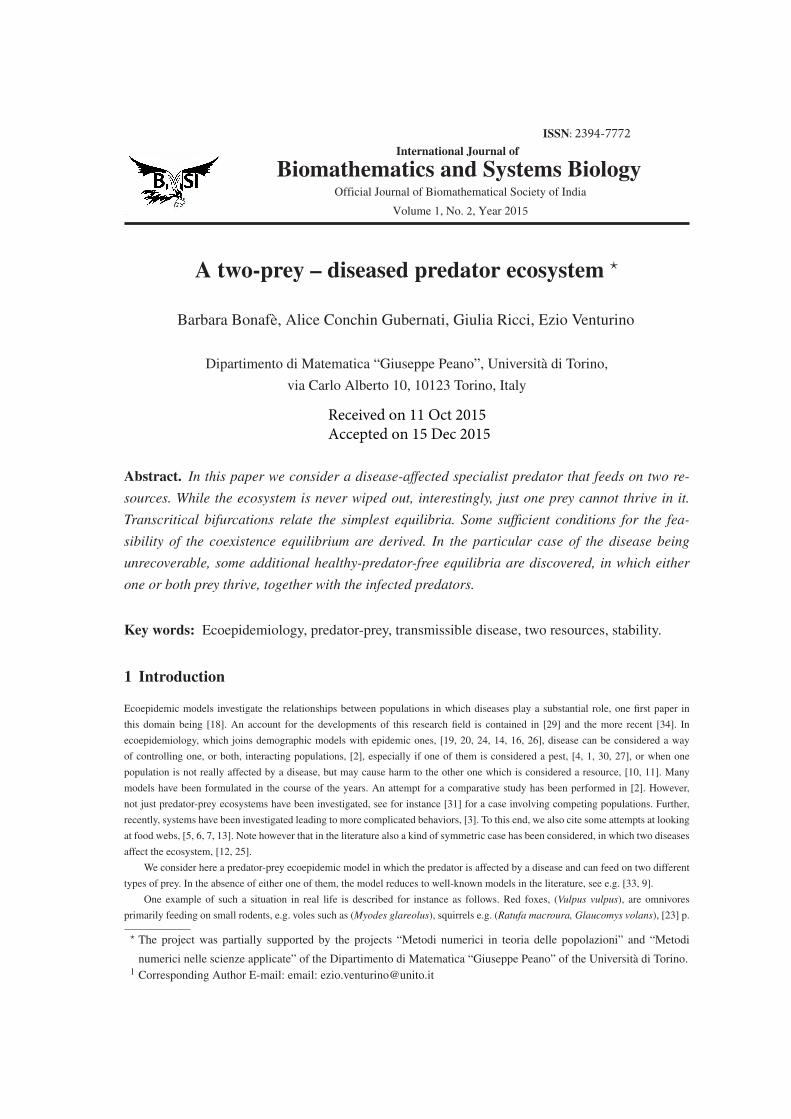
There are several possible cases that can arise, for the various positions of the hyperbola and of the straight line (3.5). However, note
that x0 > 0. Three cases are possible, reported in Figures 1-3. In each picture, note that we show the three possible positions of the
straight line (3.5). We consider in particular Figure 1. In this case observe that we are assuming D 6= 0, y0 > 0, R2 > R1, respectively
corresponding to
f m 6= c(m+µ), c(m+µ−ν)> m f , c(m+µ+ν)> f m.
There are four possible positions for the straight line (3.5), which may lead however to further subcases.
4 B. Bonafe, A. Conchin Gubernati, G. Ricci, E. Venturino
Fig. 1 An example: the hyperbola with y0 > 0. For the discussion of the possible intersections with the straight line,
see the main body of the paper.
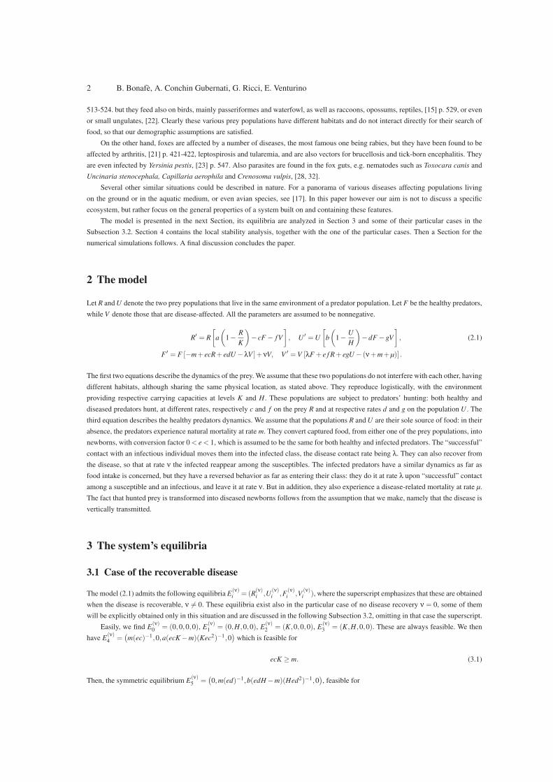
Fig. 2 A second example: another hyperbola with y0 > 0. Here for the straight line indicated by r2 in the body of the
paper, either no intersection in the first quadrant exists or exactly one is shown in the picture, but there could be two or
none if Z > R2. The straight line r4 instead is shown to have two feasible intersections if R1 < Z < R2.
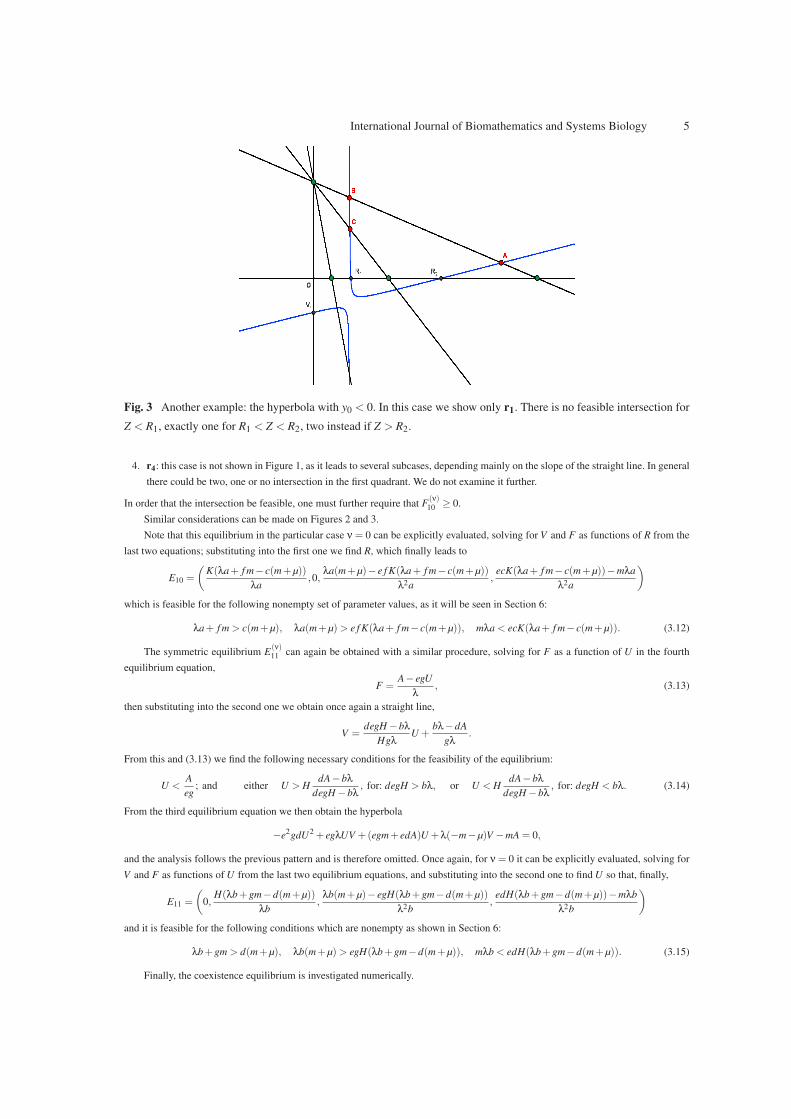
1. r1: in this case there is least one feasible intersection with the hyperbola, for j > 0, w > 0, i.e.
ce f K > aλ, aλ > cA. (3.9)
2. r2: there is exactly one intersection in the first quadrant for j < 0, w > 0 and R1 < Z < R2, i.e.
ce f K < aλ,m
ec< K
cA−aλ
ce f K −aλ<
A
e f. (3.10)
But further, for Z < R1 there is no intersection in the first quadrant, while there are two, not shown in Figure 1, for Z > R2
ce f K < aλ, KcA−aλ
ce f K −aλ>
A
e f. (3.11)
3. r3: for j < 0, w < 0, i.e. ce f K < aλ, aλ < cA, there are no feasible intersections.
International Journal of Biomathematics and Systems Biology 5
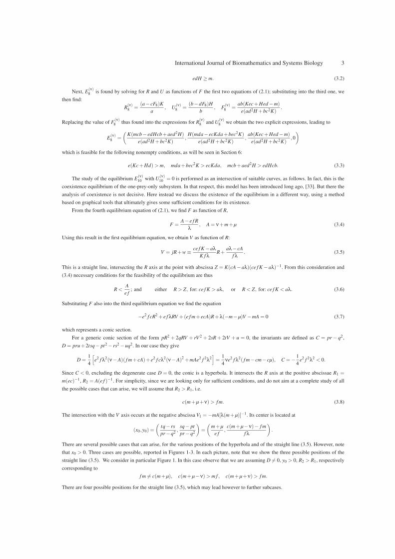
Fig. 3 Another example: the hyperbola with y0 < 0. In this case we show only r1. There is no feasible intersection for
Z < R1, exactly one for R1 < Z < R2, two instead if Z > R2.
4. r4: this case is not shown in Figure 1, as it leads to several subcases, depending mainly on the slope of the straight line. In general
there could be two, one or no intersection in the first quadrant. We do not examine it further.
In order that the intersection be feasible, one must further require that F(ν)10 ≥ 0.
Similar considerations can be made on Figures 2 and 3.
Note that this equilibrium in the particular case ν = 0 can be explicitly evaluated, solving for V and F as functions of R from the
last two equations; substituting into the first one we find R, which finally leads to
E10 =
(K(λa+ f m− c(m+µ))
λa,0,
λa(m+µ)− e f K(λa+ f m− c(m+µ))
λ2a,
ecK(λa+ f m− c(m+µ))−mλa
λ2a
)
which is feasible for the following nonempty set of parameter values, as it will be seen in Section 6:
λa+ f m > c(m+µ), λa(m+µ)> e f K(λa+ f m− c(m+µ)), mλa < ecK(λa+ f m− c(m+µ)). (3.12)
The symmetric equilibrium E(ν)11 can again be obtained with a similar procedure, solving for F as a function of U in the fourth
equilibrium equation,
F =A− egU
λ, (3.13)
then substituting into the second one we obtain once again a straight line,
V =degH −bλ
HgλU +
bλ−dA
gλ.
From this and (3.13) we find the following necessary conditions for the feasibility of the equilibrium:
U <A
eg; and either U > H
dA−bλ
degH −bλ, for: degH > bλ, or U < H
dA−bλ
degH −bλ, for: degH < bλ. (3.14)
From the third equilibrium equation we then obtain the hyperbola
−e2gdU2 + egλUV +(egm+ edA)U +λ(−m−µ)V −mA = 0,
and the analysis follows the previous pattern and is therefore omitted. Once again, for ν = 0 it can be explicitly evaluated, solving for
V and F as functions of U from the last two equilibrium equations, and substituting into the second one to find U so that, finally,
E11 =
(0,
H(λb+gm−d(m+µ))
λb,
λb(m+µ)− egH(λb+gm−d(m+µ))
λ2b,
edH(λb+gm−d(m+µ))−mλb
λ2b
)
and it is feasible for the following conditions which are nonempty as shown in Section 6:
λb+gm > d(m+µ), λb(m+µ)> egH(λb+gm−d(m+µ)), mλb < edH(λb+gm−d(m+µ)). (3.15)
Finally, the coexistence equilibrium is investigated numerically.
6 B. Bonafe, A. Conchin Gubernati, G. Ricci, E. Venturino
3.2 The particular cases
Three new equilibria arise when ν = 0. Easily, we find
E6 =
(m+µ
e f,0,0,
a(e f K − (m+µ))
Ke f 2
), E7 =
(0,
m+µ
eg,0,
b(egH − (m+µ))
Heg2
),
with respective feasibility conditions given by
e f K > m+µ, egH > m+µ. (3.16)
Further, solving for R and U as functions of F from the first two equations and substituting into the third one, we find V , which leads
to the new equilibrium
E9 =
(K(m f b− e f gHb+aeg2H +µ f b)
e(ag2H +b f 2K),
H(mga− e f gKa+be f 2K +µga)
e(ag2H +b f 2K),0,
ab(e f K + egH −m−µ)
e(ag2H +b f 2K)
),
which is feasible for
e(K f +Hg)> m+µ, mga+be f 2K +µga > e f gKa, m f b+aeg2H +µ f b > e f gHb. (3.17)
4 Stability
The Jacobian J(R,U,F,V ) of (2.1) is
J =
a(1−2 R
K
)− cF − fV 0 −cR − f R
0 b(1−2 U
H
)−dF −gV −dU −gU
ecF edF −m+ ecR+ edU −λV −λF +ν
e fV egV λV λF + e f R+ egU −ν− (m+µ)
(4.1)
It is easily established that the equilibria E(ν)0 , E
(ν)1 , E
(ν)2 , are always unstable; indeed they have respectively the following sets of
eigenvalues: γ1 = a, γ2 = b, γ3 =−m, γ4 =−(ν+m+µ); γ1 = a, γ2 =−b, γ3 = edH −m, γ4 = egH − (ν+m+µ); γ1 =−a, γ2 = b,
γ3 = ecK −m, γ4 = e f K − (ν+m+µ).
For E(ν)3 we have instead γ1 =−a, γ2 =−b, γ3 = ecK + edH −m, γ4 = e f K + egH − (ν+m+µ), giving the stability conditions
e < min
{m
cK +dH,
µ+m+ν
f K +gH
}(4.2)
For all the former equilibria, no Hopf bifurcations can arise, as the eigenvalues are all real.
For E(ν)4 , two eigenvalues are explicit,
γ1 = b−ad(ecK −m)
Kec2, γ2 =
λa(ecK −m)
Kec2+
f m
c−ν− (m+µ)
while the Routh-Hurwitz conditions for the remaining minor J are easily seen to be satisfied, in view of the feasibility condition (3.1):
−tr(J) =am
ecK> 0, det(J) =
am(ecK −m)
ecK> 0.
Stability depends only on the sign of the first two eigenvalues, giving the conditions:
b <ad(ecK −m)
Kec2,
ecK(λa+ f m)−λam
Kec2< ν+m+µ. (4.3)
At E(ν)5 we find again two explicit eigenvalues,
γ1 = a−bc(edH −m)
Hed2, γ2 =
λb(edH −m)
Hed2+
gm
d−ν− (m+µ)
International Journal of Biomathematics and Systems Biology 7
while the Routh-Hurwitz conditions for the remaining minor once again hold, bH−1U(ν)5 > 0, ed2U
(ν)5 F
(ν)5 > 0. In summary, the
stability conditions are thus:
a <bc(edH −m)
Hed2,
edH(λb+gm)−λbm
Hed2< ν+m+µ. (4.4)
Also for the equilibria E(ν)i , i= 4,5 there cannot be Hopf bifurcations, as the traces of the 2 by 2 minors are always stricly positive.
At E(ν)8 one eigenvalue is assessed immediately, γ1 = λF
(ν)8 +e f R
(ν)8 +egU
(ν)8 − (ν+m+µ). The Routh-Hurwitz criterion on the
remaining minor J of order 3 gives
−tr(J) =aR
(ν)8
K+
bU(ν)8
H> 0, −det(J) =
[ad2e
K+
bc2e
H
]R(ν)8 U
(ν)8 F
(ν)8 > 0, M2(J) =
abR(ν)8 U
(ν)8
HK+[ed2U
(ν)8 + ec2R
(ν)8
]F(ν)8 ,
where M2 represents the sum of the principal minors of order 2 of J. It follows also
−tr(J)M2(J)+det(J) =a2b(R
(ν)8 )2U
(ν)8
HK2+
ab2R(ν)8 (U
(ν)8 )2
H2K+
bd2e(U(ν)8 )2F
(ν)8
H+
ac2e(R(ν)8 )2F
(ν)8
K> 0
so that stability depends only on the first eigenvalue, giving the condition:
λF(ν)8 + e f R
(ν)8 + egU
(ν)8 < ν+m+µ. (4.5)
E(ν)10 has also an explicit eigenvalue γ1 = b− dF
(ν)10 − gV
(ν)10 , the Routh-Hurwitz conditions on the remaining minor J are rather
complicated, but some information can be gathered, for instance,
−tr(J) =aR
(ν)10
K+ν
V(ν)10
F(ν)10
> 0, −det(J) = R(ν)10 V
(ν)10
[λ2 aF
(ν)10
K−λ
aν
K+ e f ν
(c+ f
V(ν)10
F(ν)10
)],
M2(J) = c2eR(ν)10 F
(ν)10 +λ2F
(ν)10 V
(ν)10 + e f 2R
(ν)10 V
(ν)10 −λνV
(ν)10 +
aν
KF(ν)10
R(ν)10 V
(ν)10 ,
but for the last Routh-Hurwitz condition the expression is somewhat more involved and therefore omitted. Note that the sign of det(J)
must be negative, which gives an additional necessary stability condition on top of the one provided by the first eigenvalue,
λ2 aF(ν)10
K+ e f ν
(c+ f
V(ν)10
F(ν)10
)< λ
aν
K, b < dF
(ν)10 +gV
(ν)10 . (4.6)
For the specular equilibrium E(ν)11 similar considerations hold, which are omitted.
Remark. Note that equilibria E(ν)4 and E
(ν)5 are mutually exclusive, as their first stability conditions can be rewritten as
ecK(bc−ad)+adm < 0, edH(ad −bc)+bcm < 0,
so that no matter what the sign of the term ad − bc is, either one of the two must be positive, making the corresponding stability
condition impossible. For similar reasons, also E(ν)3 is incompatible with both E
(ν)4 and E
(ν)5 ; if E
(ν)3 is stable, neither E
(ν)4 nor E
(ν)5 can
be feasible, compare the first of (4.2) with (3.1) and (3.2).
4.1 The particular cases
For the additional equilibria arising for ν = 0 examined in Subsection 3.2, the stability can be assessed as follows.
E6 has the two explicit eigenvalues, γ1 =−m+ ecR6 −λV6, γ2 = b−gV6, while the remaining minor J of order 2 shows that the
Routh-Hurwitz conditions hold, −tr(J) =aR6
K> 0 and det(J) = e f 2R6V6 > 0. The stability conditions are
ecm+µ
e f< m+λ
a(e f K − (m+µ))
Ke f 2, b < g
a(e f K − (m+µ))
Ke f 2. (4.7)
For the symmetric case E7 we obtain similarly two eigenvalues γ1 =−m+edU7−λV7, γ2 = a− fV7 and again the Routh-Hurwitz
conditions hold, giving the stability conditions
8 B. Bonafe, A. Conchin Gubernati, G. Ricci, E. Venturino
b(egH − (m+µ))
Heg2> max
{d
m+µ
λg−
m
λ,
a
f
}. (4.8)
Again for these equilibria Hopf bifurcations cannot arise, since the traces of the submatrices never vanish.
For the equilibrium E9 one eigenvalue is γ1 =−m+ ecR9 + edU9 −λV9; the Routh-Hurwitz criterion on the remaining minor J∗
of order 3 gives:
−tr(J∗) =aR9
K+
bU9
H> 0, −det(J∗) = f R9
be fU9V9
H+gU9
aegR9V9
K> 0, M2(J
∗) =abR9U9
HK+ eg2U9V9 + e f 2R9V9
from which it follows
−tr(J∗)M2(J∗)+det(J∗) =
a2bR29U9
HK2+
ab2R9U29
H2K+
beg2U29 V9
H+
ae f 2R29V9
K> 0,
thereby satisfying the conditions for negative real part eigenvalues. Stability is ensured by
ecK(m f b− e f gHb+aeg2H +µ f b)
e(ag2H +b f 2K)+ ed
H(mga− e f gKa+be f 2K +µga)
e(ag2H +b f 2K)< m+λ
ab(e f K + egH −m−µ)
e(ag2H +b f 2K). (4.9)
E10 has also an explicit eigenvalue γ1 = b−dF10 −gV10, the Routh-Hurwitz conditions on the remaining minor J0 are once again
seen to be satisfied,
−tr(J0) =aR10
K> 0, −det(J0) =
λ2aR10F10V10
K> 0, M2(J
0) = c2eR10F10 +λ2F10V10 + e f 2R10V10,
and thus
−tr(J0)M2(J0)+det(J0) =
ac2eR210F10
K+
ae f 2R210V10
K> 0.
The stability condition is
b < dλa(m+µ)− e f K(λa+ f m− c(m+µ))
λ2a+g
ecK(λa+ f m− c(m+µ))−mλa
λ2a. (4.10)
At E11 similarly we find the stability condition
a < cλb(m+µ)− egH(λb+gm−d(m+µ))
λ2b+ f
edH(λb+gm−d(m+µ))−mλb
λ2b. (4.11)
Also for the equilibria Ei, i = 9,10,11, no Hopf bifurcations can arise.
5 Global stability
We establish at first that the system’s trajectories are bounded, by defining the total ecosystem population W = R+U +F +V . On
summing the equations in (2.1) we find, for an arbitrary 0 < η < m,
W ′+ηW = (a+η)R−a
KR2 +(b+η)U −
b
HU2 +(e−1)[cFR+ fV R+dFU +gVU ]+ (F +V )(η−m)−µV ≤ L
where L = 14[(a+η)2Ka−1 +(b+η)2Hb−1] is obtained as the sum of the maxima of the two parabolae in R and U , since in view of
the restriction e < 1 all the remaining terms on the right hand side can be eliminated. From the differential inequality it follows
W ≤W (0)exp(−ηt)+Lη−1[1− exp(−ηt)]≤ max{W (0),Lη−1}.
We examine now each equilibrium of the system. Consider at first E(ν)3 and the following associated function:
L3(R,U,F,V ) = αK
[R−K
K− ln
(1+
R−K
K
)]+βH
[U −H
H− ln
(1+
U −H
H
)]+ γF +δV,
where here and in what follows α, β, γ and δ are arbitrary nonnegative constants. Evidently, L3(E(ν)3 ) = 0 and in the whole positive
cone in R4, L3 ≥ 0. We now establish that this function is a Lyapunov function, by showing that its time derivative is nonpositive.
Using (2.1), we find
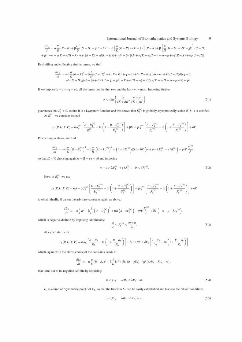
International Journal of Biomathematics and Systems Biology 9
dL3
dt= α
R′
R(R−K)+β
U ′
U(U −H)+ γF ′+δV ′ = α
[ a
K(K −R)− cF − fV
](R−K)+β
[b
H(H −U)−dF −gV
](U −H)
+γF [−m+ ecK + edH −λV + ec(R−K)+ ed(U −H)]+ γνV +δV [λF + e f K + egH −ν−m−µ+ e f (R−K)+ eg(U −H)] .
Reshuffling and collecting similar terms, we find
dL3
dt=−α
a
K(R−K)2 −β
b
H(U −H)2 +F(R−K)c(eγ−α)+V (R−K) f (eδ−α)+F(U −H)d(eγ−β)
+V (U −H)g(eδ−β)+FV λ(δ− γ)+ γF(ecK + edH −m)+V [δ(e f K + egH −m−µ−ν)+ γν].
If we impose α = β = eγ = eδ, all the terms but the first two and the last two vanish. Imposing further
e < min
{m
cK +dH,
m+µ
f K +gH
}(5.1)
guarantees that L′3 < 0, so that it is a Lyapunov function and this shows that E
(ν)3 is globally asymptotically stable if (5.1) is satisfied.
At E(ν)4 we consider instead
L4(R,U,F,V ) = αR(ν)4
[R−R
(ν)4
R(ν)4
− ln
(1+
R−R(ν)4
R(ν)4
)]+βU + γF
(ν)4
[F −F
(ν)4
F(ν)4
− ln
(1+
F −F(ν)4
F(ν)4
)]+δV.
Proceeding as above, we find
dL4
dt=−α
a
K
(R−R
(ν)4
)2
−βb
H
(U −U
(ν)4
)2
+(
b−dF(ν)4
)βU −δV
(m+µ−λF
(ν)4 − e f R
(ν)4
)− γνV
F(ν)4
F,
so that L′4 ≤ 0 choosing again α = β = eγ = eδ and imposing
m+µ > λF(ν)4 + e f R
(ν)4 , b < dF
(ν)4 . (5.2)
Next, at E(ν)5 we use
L5(R,U,F,V ) = αR+βU(ν)5
[U −U
(ν)5
U(ν)5
− ln
(1+
U −U(ν)5
U(ν)5
)]+ γF
(ν)5
[F −F
(ν)5
F(ν)5
− ln
(1+
F −F(ν)5
F(ν)5
)]+δV,
to obtain finally, if we set the arbitrary constants again as above,
dL5
dt=−α
a
KR2 −β
b
H
(U −U
(ν)5
)2
+αR(
a− cF(ν)5
)− γνV
F(ν)5
F+δV
(−m−µ+λF
(ν)5
),
which is negative definite by imposing additionally:a
c≤ F
(ν)5 ≤
m+µ
λ. (5.3)
At E6 we start with
L6(R,U,F,V ) = αR6
[R−R6
R6− ln
(1+
R−R6
R6
)]+βU + γF +δV6
[V −V6
V6− ln
(1+
V −V6
V6
)],
which, again with the above choice of the constants, leads to
dL6
dt=−α
a
K(R−R6)
2 −βb
HU2 +βU (b−gV6)+ γF (ecR6 −λV6 −m) ,
that turns out to be negative definite by requiring:
b < gV6, ecR6 < λV6 +m. (5.4)
E7 is a kind of “symmetric point” of E6, so that the function L7 can be easily established and leads to the “dual” conditions
a < fV7, edU7 < λV7 +m. (5.5)
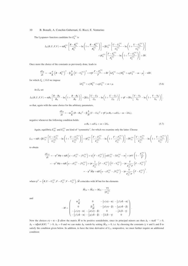
10 B. Bonafe, A. Conchin Gubernati, G. Ricci, E. Venturino
The Lyapunov function candidate for E(ν)8 is
L8(R,U,F,V ) = αR(ν)8
[R−R
(ν)8
R(ν)8
− ln
(1+
R−R(ν)8
R(ν)8
)]+βU
(ν)8
[U −U
(ν)8
U(ν)8
− ln
(1+
U −U(ν)8
U(ν)8
)]
+γF(ν)8
[F −F
(ν)8
F(ν)8
− ln
(1+
F −F(ν)8
F(ν)8
)]+δV.
Once more the choice of the constants as previously done, leads to
dL8
dt=−α
a
K
(R−R
(ν)8
)2
−βb
H
(U −U
(ν)8
)2
+νγVF −F
(ν)8
F+δV
[λF
(ν)8 + e f R
(ν)8 + egU
(ν)8 −m−µ
]−νδV,
for which L′8 ≤ 0 if we impose
λF(ν)8 + e f R
(ν)8 + egU
(ν)8 < m+µ. (5.6)
At E9 set
L9(R,U,F,V ) = αR9
[R−R9
R9− ln
(1+
R−R9
R9
)]+βU9
[U −U9
U9− ln
(1+
U −U9
U9
)]+ γF +δV9
[V −V9
V9− ln
(1+
V −V9
V9
)].
so that, again with the same choice for the arbitrary parameters,
dL9
dt=−α
a
K(R−R9)
2 −βb
H(U −U9)
2 + γF(ecR9 + edU9 −m−λV9),
negative whenever the following condition holds:
ecR9 + edU9 < m+λV9. (5.7)
Again, equilibria E(ν)10 and E
(ν)11 are kind of “symmetric”, for which we examine only the latter. Choose
L11 =αR+βU(ν)11
[U −U
(ν)11
U(ν)11
− ln
(1+
U −U(ν)11
U(ν)11
)]+γF
(ν)11
[F −F
(ν)11
F(ν)11
− ln
(1+
F −F(ν)11
F(ν)11
)]+δV
(ν)11
[V −V
(ν)11
V(ν)11
− ln
(1+
V −V(ν)11
V(ν)11
)].
to obtain
dL11
dt=−yT My+αR
(a− cF
(ν)11 − fV
(ν)11
)+ γ(
F −F(ν)11
)[edU
(ν)11 −λV
(ν)11 −m
]+ γνV
(1−
F(ν)11
F
)
=−yT My+αR(
a− cF(ν)11 − fV
(ν)11
)+ γν
1
F(ν)11
(F −F
(ν)11
)(V −V
(ν)11
)− γν
V
F(ν)11 F
(F −F
(ν)11
)2
=−yT My+αR(
a− cF(ν)11 − fV
(ν)11
)− γν
V
F(ν)11 F
(F −F
(ν)11
)2
,
where yT =(
R,U −U(ν)11 ,F −F
(ν)11 ,V −V
(ν)11
), M coincides with M but for the elements
M34 = M43 = M43 −νγ
2F(ν)11
and
−M =
αa
K0 − 1
2c(eγ−α) − 1
2f (eδ−α)
0 βb
H− 1
2d(eγ−β) − 1
2g(eδ−β)
− 12
c(eγ−α) − 12
d(eγ−β) 0 − 12
λ(δ− γ)
− 12
f (eδ−α) − 12
g(eδ−β) − 12
λ(δ− γ) 0
.
Now the choices eγ = α = β allow the matrix M to be positive semidefinite, since its principal minors are then ∆1 = αaK−1 > 0,
∆2 = αβab(KH)−1 > 0, ∆3 = 0 and we can make ∆4 vanish by setting M34 = 0, i.e. by choosing the constants γ, ν and λ and δ to
satisfy the condition given below. In addition, to have the time derivative of L11 nonpositive, we must further require an additional
condition:
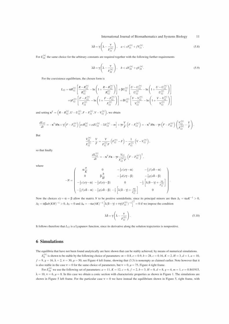
International Journal of Biomathematics and Systems Biology 11
λδ = γ
(λ−
ν
F(ν)11
), a < cF
(ν)11 + fV
(ν)11 . (5.8)
For E(ν)10 the same choice for the arbitrary constants are required together with the following further requirements
λδ = γ
(λ−
ν
F(ν)10
), b < dF
(ν)10 +gV
(ν)10 . (5.9)
For the coexistence equilibrium, the chosen form is
L12 = αR(ν)12
[R−R
(ν)12
R(ν)12
− ln
(1+
R−R(ν)12
R(ν)12
)]+βU
(ν)12
[U −U
(ν)12
U(ν)12
− ln
(1+
U −U(ν)12
U(ν)12
)]
+γF(ν)12
[F −F
(ν)12
F(ν)12
− ln
(1+
F −F(ν)12
F(ν)12
)]+δV
(ν)12
[V −V
(ν)12
V(ν)12
− ln
(1+
V −V(ν)12
V(ν)12
)]
and setting xT =(
R−R(ν)12 ,U −U
(ν)12 ,F −F
(ν)12 ,V −V
(ν)12
), we obtain
dL12
dt=−xT Mx+ γ
(F −F
(ν)12
)[ecR
(ν)12 + edU
(ν)12 −λV
(ν)12 −m
]+ γν
V
F
(F −F
(ν)12
)=−xT Mx− γν
(F −F
(ν)12
)(V(ν)12
F(ν)12
−V
F
).
But
V(ν)12
F(ν)12
−V
F=
V
F(ν)12 F
(F(ν)12 −F
)−
1
F(ν)12
(V −V
(ν)12
),
so that finally
dL(ν)12
dt=−xT Nx− γν
V12
F(ν)12 F
(F −F
(ν)12
)2
,
where
−N =
αa
K0 − 1
2c(eγ−α) − 1
2f (eδ−α)
0 βb
H− 1
2d(eγ−β) − 1
2g(eδ−β)
− 12
c(eγ−α) − 12
d(eγ−β) 0 − 12
[λ(δ− γ)+ νγ
F(ν)12
]
− 12
f (eδ−α) − 12
g(eδ−β) − 12
[λ(δ− γ)+ νγ
F(ν)12
]0
.
Now the choices eγ = α = β allow the matrix N to be positive semidefinite, since its principal minors are then ∆1 = αaK−1 > 0,
∆2 = αβab(KH)−1 > 0, ∆3 = 0 and ∆4 =−αa(4K)−1[λ(δ− γ)+νγ(F
(ν)12 )−1
]2
= 0 if we impose the condition
λδ = γ
(λ−
ν
F(ν)12
). (5.10)
It follows therefore that L12 is a Lyapunov function, since its derivative along the solution trajectories is nonpositive.
6 Simulations
The equilibria that have not been found analytically are here shown that can be stably achieved, by means of numerical simulations.
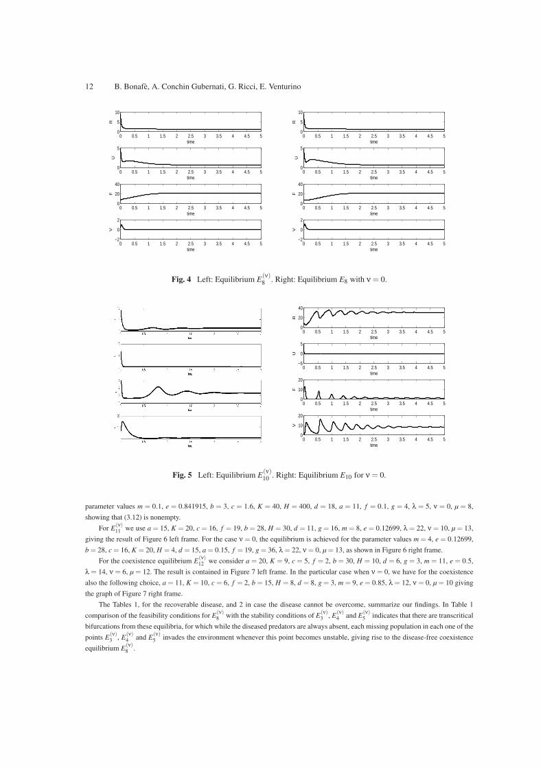
E(ν)8 is shown to be stable by the following choice of parameters: m = 0.8, e = 0.9, b = 28, c = 0.16, K = 2, H = 3, d = 1, a = 10,
f = 9, g = 16, λ = 2, ν = 30, µ = 50, see Figure 4 left frame, showing that (3.3) is nonempty as claimed earlier. Note however that it
is also stable in the case ν = 0 for the same choice of parameters, but ν = 0, µ = 75, Figure 4 right frame.
For E(ν)10 we use the following set of parameters: a = 11, K = 12, c = 6, f = 2, b = 3, H = 8, d = 8, g = 4, m = 1, e = 0.841915,
λ = 10, ν = 6, µ = 8. In this case we obtain a conic section with characteristic properties as shown in Figure 1. The simulations are
shown in Figure 5 left frame. For the particular case ν = 0 we have instead the equilibrium shown in Figure 5, right frame, with
12 B. Bonafe, A. Conchin Gubernati, G. Ricci, E. Venturino
0 0.5 1 1.5 2 2.5 3 3.5 4 4.5 50
5
10R
time
0 0.5 1 1.5 2 2.5 3 3.5 4 4.5 50
5
time
U
0 0.5 1 1.5 2 2.5 3 3.5 4 4.5 50
20
40
time
F
0 0.5 1 1.5 2 2.5 3 3.5 4 4.5 5−2
0
2
time
V
0 0.5 1 1.5 2 2.5 3 3.5 4 4.5 50
5
10
R
time
0 0.5 1 1.5 2 2.5 3 3.5 4 4.5 50
5
time
U
0 0.5 1 1.5 2 2.5 3 3.5 4 4.5 50
20
40
time
F
0 0.5 1 1.5 2 2.5 3 3.5 4 4.5 5−2
0
2
time
V
Fig. 4 Left: Equilibrium E(ν)8 . Right: Equilibrium E8 with ν = 0.
0 0.5 1 1.5 2 2.5 3 3.5 4 4.5 50
20
40
R
time
0 0.5 1 1.5 2 2.5 3 3.5 4 4.5 5−5
0
5
time
U
0 0.5 1 1.5 2 2.5 3 3.5 4 4.5 50
10
20
time
F
0 0.5 1 1.5 2 2.5 3 3.5 4 4.5 50
10
20
time
V
Fig. 5 Left: Equilibrium E(ν)10 . Right: Equilibrium E10 for ν = 0.
parameter values m = 0.1, e = 0.841915, b = 3, c = 1.6, K = 40, H = 400, d = 18, a = 11, f = 0.1, g = 4, λ = 5, ν = 0, µ = 8,
showing that (3.12) is nonempty.
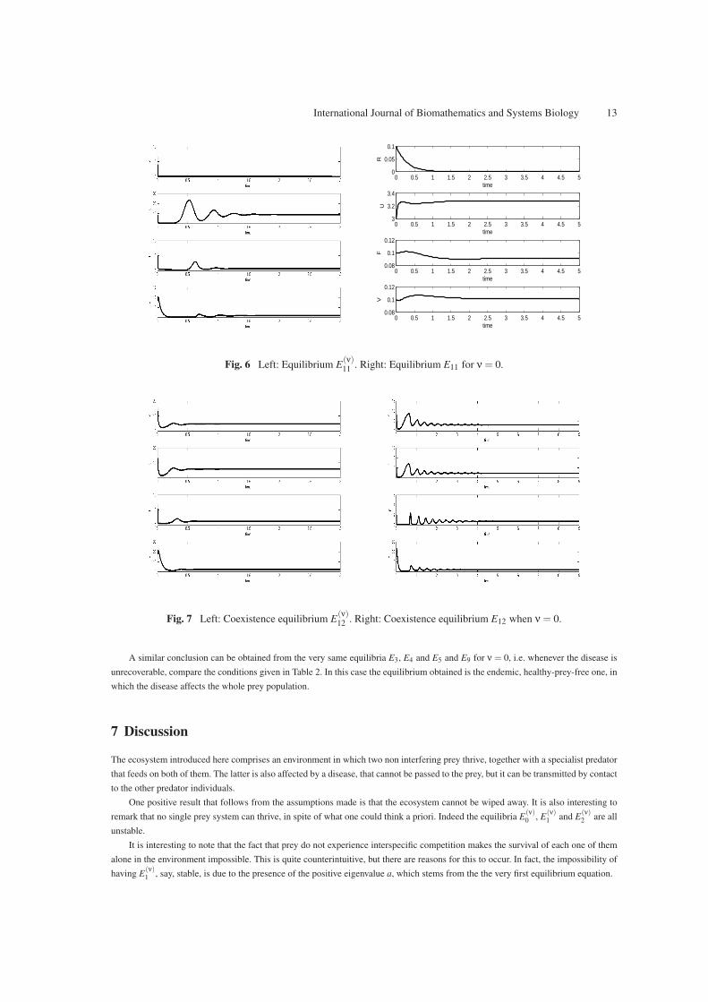
For E(ν)11 we use a = 15, K = 20, c = 16, f = 19, b = 28, H = 30, d = 11, g = 16, m = 8, e = 0.12699, λ = 22, ν = 10, µ = 13,
giving the result of Figure 6 left frame. For the case ν = 0, the equilibrium is achieved for the parameter values m = 4, e = 0.12699,
b = 28, c = 16, K = 20, H = 4, d = 15, a = 0.15, f = 19, g = 36, λ = 22, ν = 0, µ = 13, as shown in Figure 6 right frame.
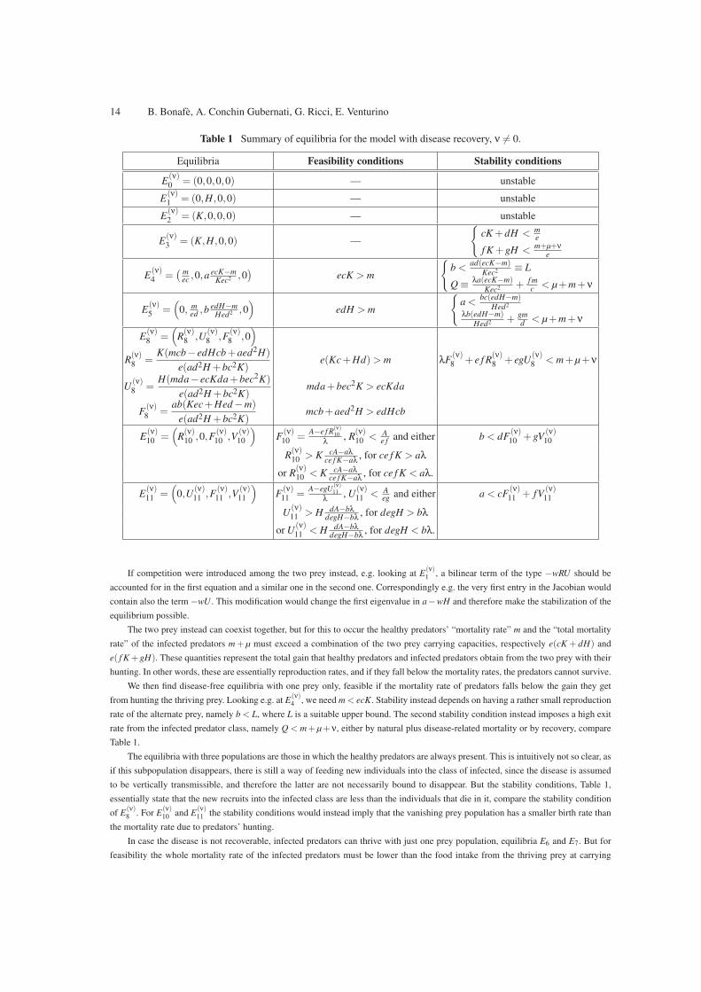
For the coexistence equilibrium E(ν)12 we consider a = 20, K = 9, c = 5, f = 2, b = 30, H = 10, d = 6, g = 3, m = 11, e = 0.5,
λ = 14, ν = 6, µ = 12. The result is contained in Figure 7 left frame. In the particular case when ν = 0, we have for the coexistence
also the following choice, a = 11, K = 10, c = 6, f = 2, b = 15, H = 8, d = 8, g = 3, m = 9, e = 0.85, λ = 12, ν = 0, µ = 10 giving
the graph of Figure 7 right frame.
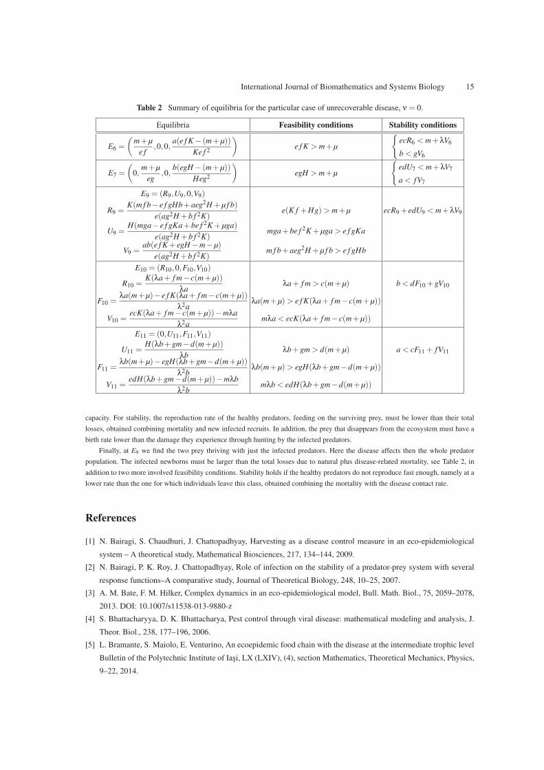
The Tables 1, for the recoverable disease, and 2 in case the disease cannot be overcome, summarize our findings. In Table 1
comparison of the feasibility conditions for E(ν)8 with the stability conditions of E
(ν)3 , E
(ν)4 and E
(ν)5 indicates that there are transcritical
bifurcations from these equilibria, for which while the diseased predators are always absent, each missing population in each one of the
points E(ν)3 , E
(ν)4 and E
(ν)5 invades the environment whenever this point becomes unstable, giving rise to the disease-free coexistence
equilibrium E(ν)8 .
International Journal of Biomathematics and Systems Biology 13
0 0.5 1 1.5 2 2.5 3 3.5 4 4.5 50
0.05
0.1
R
time
0 0.5 1 1.5 2 2.5 3 3.5 4 4.5 53
3.2
3.4
time
U
0 0.5 1 1.5 2 2.5 3 3.5 4 4.5 50.08
0.1
0.12
time
F
0 0.5 1 1.5 2 2.5 3 3.5 4 4.5 50.08
0.1
0.12
time
V
Fig. 6 Left: Equilibrium E(ν)11 . Right: Equilibrium E11 for ν = 0.
Fig. 7 Left: Coexistence equilibrium E(ν)12 . Right: Coexistence equilibrium E12 when ν = 0.
A similar conclusion can be obtained from the very same equilibria E3, E4 and E5 and E9 for ν = 0, i.e. whenever the disease is
unrecoverable, compare the conditions given in Table 2. In this case the equilibrium obtained is the endemic, healthy-prey-free one, in
which the disease affects the whole prey population.
7 Discussion
The ecosystem introduced here comprises an environment in which two non interfering prey thrive, together with a specialist predator
that feeds on both of them. The latter is also affected by a disease, that cannot be passed to the prey, but it can be transmitted by contact
to the other predator individuals.
One positive result that follows from the assumptions made is that the ecosystem cannot be wiped away. It is also interesting to
remark that no single prey system can thrive, in spite of what one could think a priori. Indeed the equilibria E(ν)0 , E
(ν)1 and E
(ν)2 are all
unstable.
It is interesting to note that the fact that prey do not experience interspecific competition makes the survival of each one of them
alone in the environment impossible. This is quite counterintuitive, but there are reasons for this to occur. In fact, the impossibility of
having E(ν)1 , say, stable, is due to the presence of the positive eigenvalue a, which stems from the the very first equilibrium equation.
14 B. Bonafe, A. Conchin Gubernati, G. Ricci, E. Venturino
Table 1 Summary of equilibria for the model with disease recovery, ν 6= 0.
Equilibria Feasibility conditions Stability conditions
E(ν)0 = (0,0,0,0) — unstable
E(ν)1 = (0,H,0,0) — unstable
E(ν)2 = (K,0,0,0) — unstable
E(ν)3 = (K,H,0,0) —
{cK +dH <
me
f K +gH <m+µ+ν
e
E(ν)4 =
(mec ,0,a
ecK−mKec2 ,0
)ecK > m
{b <
ad(ecK−m)Kec2 ≡ L
Q ≡λa(ecK−m)
Kec2 + f mc < µ+m+ν
E(ν)5 =
(0, m
ed ,bedH−m
Hed2 ,0)
edH > m
{a <
bc(edH−m)Hed2
λb(edH−m)Hed2 + gm
d < µ+m+ν
E(ν)8 =
(R(ν)8 ,U
(ν)8 ,F
(ν)8 ,0
)
R(ν)8 =
K(mcb− edHcb+aed2H)
e(ad2H +bc2K)e(Kc+Hd)> m λF
(ν)8 + e f R
(ν)8 + egU
(ν)8 < m+µ+ν
U(ν)8 =
H(mda− ecKda+bec2K)
e(ad2H +bc2K)mda+bec2K > ecKda
F(ν)8 =
ab(Kec+Hed −m)
e(ad2H +bc2K)mcb+aed2H > edHcb
E(ν)10 =
(R(ν)10 ,0,F
(ν)10 ,V
(ν)10
)F(ν)10 =
A−e f R(ν)10
λ, R
(ν)10 <
Ae f and either b < dF
(ν)10 +gV
(ν)10
R(ν)10 > K cA−aλ
ce f K−aλ, for ce f K > aλ
or R(ν)10 < K cA−aλ
ce f K−aλ, for ce f K < aλ.
E(ν)11 =
(0,U
(ν)11 ,F
(ν)11 ,V
(ν)11
)F(ν)11 =
A−egU(ν)11
λ, U
(ν)11 <
Aeg and either a < cF
(ν)11 + fV
(ν)11
U(ν)11 > H dA−bλ
degH−bλ, for degH > bλ
or U(ν)11 < H dA−bλ
degH−bλ, for degH < bλ.
If competition were introduced among the two prey instead, e.g. looking at E(ν)1 , a bilinear term of the type −wRU should be
accounted for in the first equation and a similar one in the second one. Correspondingly e.g. the very first entry in the Jacobian would
contain also the term −wU . This modification would change the first eigenvalue in a−wH and therefore make the stabilization of the
equilibrium possible.
The two prey instead can coexist together, but for this to occur the healthy predators’ “mortality rate” m and the “total mortality
rate” of the infected predators m+ µ must exceed a combination of the two prey carrying capacities, respectively e(cK + dH) and
e( f K+gH). These quantities represent the total gain that healthy predators and infected predators obtain from the two prey with their
hunting. In other words, these are essentially reproduction rates, and if they fall below the mortality rates, the predators cannot survive.
We then find disease-free equilibria with one prey only, feasible if the mortality rate of predators falls below the gain they get
from hunting the thriving prey. Looking e.g. at E(ν)4 , we need m < ecK. Stability instead depends on having a rather small reproduction
rate of the alternate prey, namely b < L, where L is a suitable upper bound. The second stability condition instead imposes a high exit
rate from the infected predator class, namely Q < m+µ+ν, either by natural plus disease-related mortality or by recovery, compare
Table 1.
The equilibria with three populations are those in which the healthy predators are always present. This is intuitively not so clear, as
if this subpopulation disappears, there is still a way of feeding new individuals into the class of infected, since the disease is assumed
to be vertically transmissible, and therefore the latter are not necessarily bound to disappear. But the stability conditions, Table 1,
essentially state that the new recruits into the infected class are less than the individuals that die in it, compare the stability condition
of E(ν)8 . For E
(ν)10 and E
(ν)11 the stability conditions would instead imply that the vanishing prey population has a smaller birth rate than
the mortality rate due to predators’ hunting.
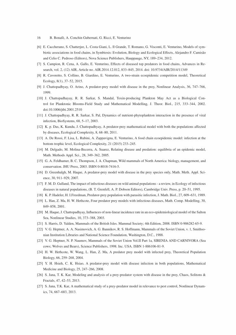
In case the disease is not recoverable, infected predators can thrive with just one prey population, equilibria E6 and E7. But for
feasibility the whole mortality rate of the infected predators must be lower than the food intake from the thriving prey at carrying
International Journal of Biomathematics and Systems Biology 15
Table 2 Summary of equilibria for the particular case of unrecoverable disease, ν = 0.
Equilibria Feasibility conditions Stability conditions
E6 =
(m+µ
e f,0,0,
a(e f K − (m+µ))
Ke f 2
)e f K > m+µ
{ecR6 < m+λV6
b < gV6
E7 =
(0,
m+µ
eg,0,
b(egH − (m+µ))
Heg2
)egH > m+µ
{edU7 < m+λV7
a < fV7
E9 = (R9,U9,0,V9)
R9 =K(m f b− e f gHb+aeg2H +µ f b)
e(ag2H +b f 2K)e(K f +Hg)> m+µ ecR9 + edU9 < m+λV9
U9 =H(mga− e f gKa+be f 2K +µga)
e(ag2H +b f 2K)mga+be f 2K +µga > e f gKa
V9 =ab(e f K + egH −m−µ)
e(ag2H +b f 2K)m f b+aeg2H +µ f b > e f gHb
E10 = (R10,0,F10,V10)
R10 =K(λa+ f m− c(m+µ))
λaλa+ f m > c(m+µ) b < dF10 +gV10
F10 =λa(m+µ)− e f K(λa+ f m− c(m+µ))
λ2aλa(m+µ)> e f K(λa+ f m− c(m+µ))
V10 =ecK(λa+ f m− c(m+µ))−mλa
λ2amλa < ecK(λa+ f m− c(m+µ))
E11 = (0,U11,F11,V11)
U11 =H(λb+gm−d(m+µ))
λbλb+gm > d(m+µ) a < cF11 + fV11
F11 =λb(m+µ)− egH(λb+gm−d(m+µ))
λ2bλb(m+µ)> egH(λb+gm−d(m+µ))
V11 =edH(λb+gm−d(m+µ))−mλb
λ2bmλb < edH(λb+gm−d(m+µ))
capacity. For stability, the reproduction rate of the healthy predators, feeding on the surviving prey, must be lower than their total
losses, obtained combining mortality and new infected recruits. In addition, the prey that disappears from the ecosystem must have a
birth rate lower than the damage they experience through hunting by the infected predators.
Finally, at E9 we find the two prey thriving with just the infected predators. Here the disease affects then the whole predator
population. The infected newborns must be larger than the total losses due to natural plus disease-related mortality, see Table 2, in
addition to two more involved feasibility conditions. Stability holds if the healthy predators do not reproduce fast enough, namely at a
lower rate than the one for which individuals leave this class, obtained combining the mortality with the disease contact rate.
References
[1] N. Bairagi, S. Chaudhuri, J. Chattopadhyay, Harvesting as a disease control measure in an eco-epidemiological
system – A theoretical study, Mathematical Biosciences, 217, 134–144, 2009.
[2] N. Bairagi, P. K. Roy, J. Chattopadhyay, Role of infection on the stability of a predator-prey system with several
response functions–A comparative study, Journal of Theoretical Biology, 248, 10–25, 2007.
[3] A. M. Bate, F. M. Hilker, Complex dynamics in an eco-epidemiological model, Bull. Math. Biol., 75, 2059–2078,
2013. DOI: 10.1007/s11538-013-9880-z
[4] S. Bhattacharyya, D. K. Bhattacharya, Pest control through viral disease: mathematical modeling and analysis, J.
Theor. Biol., 238, 177–196, 2006.
[5] L. Bramante, S. Maiolo, E. Venturino, An ecoepidemic food chain with the disease at the intermediate trophic level
Bulletin of the Polytechnic Institute of Iasi, LX (LXIV), (4), section Mathematics, Theoretical Mechanics, Physics,
9–22, 2014.
16 B. Bonafe, A. Conchin Gubernati, G. Ricci, E. Venturino
[6] E. Caccherano, S. Chatterjee, L. Costa Giani, L. Il Grande, T. Romano, G. Visconti, E. Venturino, Models of sym-
biotic associations in food chains, in Symbiosis: Evolution, Biology and Ecological Effects, Alejandro F. Camisao
and Celio C. Pedroso (Editors), Nova Science Publishers, Hauppauge, NY, 189–234, 2012.
[7] S. Campion, R. Cena, A. Gallo, E. Venturino, Effects of diseased top predators in food chains, Advances in Re-
search, vol. 2, (12) AIR, Article no. AIR.2014.12.012, 833–845, 2014. doi: 10.9734/AIR/2014/11349
[8] R. Cavoretto, S. Collino, B. Giardino, E. Venturino, A two-strain ecoepidemic competition model, Theoretical
Ecology, 8(1), 37–52, 2015.
[9] J. Chattopadhyay, O. Arino, A predator-prey model with disease in the prey, Nonlinear Analysis, 36, 747–766,
1999.
[10] J. Chattopadhayay, R. R. Sarkar, S. Mandal, Toxin-producing Plankton May Act as a Biological Con-
trol for Planktonic Blooms-Field Study and Mathematical Modelling, J. Theor. Biol., 215, 333–344, 2002.
doi:10.1006/jtbi.2001.2510
[11] J. Chattopadhyay, R. R. Sarkar, S. Pal, Dynamics of nutrient-phytoplankton interaction in the presence of viral
infection, BioSystems, 68, 5–17, 2003.
[12] K. p. Das, K. Kundu, J. Chattopadhyay, A predator-prey mathematical model with both the populations affected
by diseases, Ecological Complexity, 8, 68–80, 2011.
[13] A. De Rossi, F. Lisa, L. Rubini, A. Zappavigna, E. Venturino, A food chain ecoepidemic model: infection at the
bottom trophic level, Ecological Complexity, 21 (2015) 233–245.
[14] M. Delgado, M. Molina-Becerra, A. Suarez, Relating disease and predation: equilibria of an epidemic model,
Math. Methods Appl. Sci., 28, 349–362, 2005.
[15] G. A. Feldhamer, B. C. Thompson, J. A. Chapman, Wild mammals of North America: biology, management, and
conservation. JHU Press, 2003. ISBN 0-8018-7416-5.
[16] D. Greenhalgh, M. Haque, A predator-prey model with disease in the prey species only, Math. Meth. Appl. Sci-
ence, 30, 911–929, 2007.
[17] F. M. D. Gulland, The impact of infectious diseases on wild animal populations - a review, in Ecology of infectious
diseases in natural populations, (B. T. Grenfell, A. P. Dobson Editors), Cambridge Univ. Press, p. 20–51, 1995.
[18] K. P. Hadeler, H. I.Freedman, Predator-prey population with parasitic infection, J. Math. Biol., 27, 609–631, 1989.
[19] L. Han, Z. Ma, H. W. Hethcote, Four predator prey models with infectious diseases, Math. Comp. Modelling, 30,
849–858, 2001.
[20] M. Haque, J. Chattopadhyay, Influences of non-linear incidence rate in an eco-epidemiological model of the Salton
Sea, Nonlinear Studies, 10, 373–388, 2003.
[21] S. Harris, D. Yalden, Mammals of the British Isles. Mammal Society; 4th Edition, 2008. ISBN 0-906282-65-9.
[22] V. G. Heptner, A. A. Nasimovich, A. G. Bannikov, R. S. Hoffmann, Mammals of the Soviet Union, v. 1, Smithso-
nian Institution Libraries and National Science Foundation, Washington, D.C., 1988.
[23] V. G. Heptner, N. P. Naumov, Mammals of the Soviet Union Vol.II Part 1a, SIRENIA AND CARNIVORA (Sea
cows; Wolves and Bears), Science Publishers, 1998. Inc. USA. ISBN 1-886106-81-9.
[24] H. W. Hethcote, W. Wang, L. Han, Z. Ma, A predator prey model with infected prey, Theoretical Population
Biology, 66, 259–268, 2004.
[25] Y. H. Hsieh, C. K. Hsiao, A predator-prey model with disease infection in both populations, Mathematical
Medicine and Biology, 25, 247–266, 2008.
[26] S. Jana, T. K. Kar, Modeling and analysis of a prey-predator system with disease in the prey, Chaos, Solitons &
Fractals, 47, 42–53, 2013.
[27] S. Jana, T.K. Kar, A mathematical study of a prey-predator model in relevance to pest control, Nonlinear Dynam-
ics, 74, 667–683, 2013.
International Journal of Biomathematics and Systems Biology 17
[28] V. Lalosevic, D.; Lalosevic, I. Capo, V. Simin, A. Galfi, D. Traversa, High infection rate of zoonotic Eucoleus
aerophilus infection in foxes from Serbia, Parasite 20 (3) (5 pages) 2013. doi:10.1051/parasite/2012003. PMC
3718516. PMID 23340229
[29] H. Malchow, S. Petrovskii, E. Venturino, Spatiotemporal patterns in Ecology and Epidemiology, CRC, Boca
Raton, 2008.
[30] N. M. Oliveira, F. M. Hilker, Modelling Disease Introduction as Biological Control of Invasive Predators to Pre-
serve Endangered Prey, Bulletin of Mathematical Biology, 72, 444–468, 2010. DOI: 10.1007/s11538-009-9454-2
[31] R. A. Saenz, H. W. Hethcote, Competing species models with an infectious disease, Mathematical Biosciences
and Engineering, 3, 219–235, 2006.
[32] T. Sreter, Z. Szell, G. Marucci, E. Pozio, I. Varga, Extraintestinal nematode infections of red foxes (Vulpes vulpes)
in Hungary, Vet. Parasitol., 115(4), 329–334, 2003.
[33] E. Venturino, Epidemics in predator-prey models: disease among the prey, in O. Arino, D. Axelrod, M. Kim-
mel, M. Langlais: Mathematical Population Dynamics: Analysis of Heterogeneity, Vol. one: Theory of Epidemics,
Wuertz Publishing Ltd, Winnipeg, Canada, p. 381–393, 1995.
[34] E. Venturino, Ecoepidemiology: a more comprehensive view of population interactions, Mathematical Modelling
of Natural Phenomena, 11(1), 49–90, 2016.