Biological and Physical Assessment of Streams in Northern California: Evaluating the Effects of Global Change and Human Disturbance

by

Justin Earl Lawrence

A dissertation submitted in partial satisfaction of the

Requirements for the degree of

Doctor of Philosophy

in

Environmental Science, Policy, and Management

in the

Graduate Division

of the

University of California, Berkeley

Committee in charge:

Professor Vincent H. Resh, Chair Professor G. Mathias Kondolf

Professor Joe R. McBride

Spring 2011

Biological and Physical Assessment of Streams in Northern California: Evaluating the Effects of Global Change and Human Disturbance

Copyright 2011

by

Justin Earl Lawrence

1

Abstract

Biological and Physical Assessment of Streams in Northern California: Evaluating the Effects of

Global Change and Human Disturbance

by

Justin Earl Lawrence

Doctor of Philosophy in Environmental Science, Policy, and Management

University of California, Berkeley

Professor Vincent H. Resh, Chair

Human disturbance at global and local scales is profoundly impacting stream ecosystems in California. For example, climate change is causing notable increases in air temperature and decreases in precipitation in some regions of the state. These changes are outside the range of natural variability and are expected to intensify. Furthermore, these changes affect stream-water temperatures, stream-flow levels, and aquatic biota. Human disturbance at the local scale in California includes, but is not limited to, urbanization, the development and use of land for timber extraction and agriculture, and manipulation of habitats for recreation or for the preservation of endangered species. I examined the impacts of global change and human disturbance on stream ecosystems in Northern California at a variety of sites and using a variety of biological and physical techniques.The sites were located in five California counties, including Lake, Marin, Napa, Siskiyou, and Sonoma. Monitoring and analytical techniques for benthic macroinvertebrates used both standard and novel approaches and metrics of biological assessment. Physical techniques included surveys of channel widths and longitudinal profiles, bankfull-channel estimates, flow measurements, pebble counts, fine-sediment measurements, and large-wood inventories, which were analyzed using a variety of geomorphological and hydrological approaches. I found that: 1) the common metrics used in biological assessment will have continued applicability for biological assessment programs in Northern California and that a new metric for detecting climate-change effects could be developed; 2) stream-crossing reconstruction was causing increased patchiness of benthic-macroinvertebrate communities in the short term; 3) vineyard water-withdrawals were having an effect on stream communities that occurred after a threshold level of vineyard coverage and extent was reached; and 4) the addition of engineered, large-wood structures to streams for physical-habitat restoration increased pool frequency and caused changes in the benthic community, although the resulting levels of large wood in the channels were still lower than levels typically found in other regions of the northwestern United States.

i

TABLE OF CONTENTS

Table of Contents…………………............…………………………………………………….….i

Dedication…………………………………………………….............……………………...……ii

Acknowledgements………………………............………………………………………………iii

Introduction………………………………............………………………………………........….iv

CHAPTER 1: Long-term macroinvertebrate responses to climate change: implications for biological assessment in mediterranean-climate streams................................................................1

CHAPTER 2: Short-term impacts of stream-crossing reconstruction on forested, mountain streams in Northern California………………………………............................……......……….35

CHAPTER 3: The effects of vineyard coverage and extent on benthic macroinvertebrates in streams in Northern California……………………………………................………………...…82

CHAPTER 4: Physical-habitat restoration in the Lagunitas Creek watershed, Marin Co., California: evaluating the effects of large wood on pool formation in streams........................... 98

CHAPTER 5: Physical-habitat restoration in the Lagunitas Creek watershed, Marin Co., California: evaluating the effects of large wood on benthic macroinvertebrates……...............117

ii

DEDICATION

To my parents, Dr. John C. Lawrence, Jr. and Linda L. Lawrence forbringing me into this world and raising me well.

iii

ACKNOWLEDGMENTS

I am enormously grateful to Dr. Vincent Resh, my primary advisor, for his unwavering enthusiasm and support. Vince’s dedication to high professional standards and his love of people has been a tremendous source of inspiration. It was truly an honor to be part of his lab. I thank the members of my qualifying exam committee: Professors Joe McBride, Mary Power, Matt Kondolf, and Stephanie Carlson. I truly enjoyed my conversations with them prior to the exam, and was very impressed by their generosity. Furthermore, I thank Joe McBride for inviting me to participate in the UC Forestry Camp during all my summers in graduate school and Matt Kondolf for giving me the opportunity to take part in his river-restoration short course.I also thank Professor Elizabeth Boyer for her help getting me started with my Ph.D at Berkeley. My daily routine was greatly enriched by my fellow graduate students in the Resh Lab, including Alison Purcell, Igor Laçan, Joanie Ball, Kaua Fraiola, Kevin Lunde, Lisa Hunt, Matt Cover, Patina Mendez, and Wendy Renz. I also deeply enjoyed the friendship of other graduate students outside the lab, especially Alice Kelley, Hyojin Kim, Kristen Podolak, Mary Matella, Matteo Kausch, and Teresa Ippolito. Without such friends, life would have been far less sunny. I have many additional individuals to thank who collaborated and provided invaluable expertise and encouragement on my various research projects. I thank: Leah Bêche (UC Berkeley), Michael Barbour (Tetra Tech), Núria Bonada (University of Barcelona), Pamela Silver (Pennsylvania State University), Peter Ode (Surface Water Ambient Monitoring Program), and Rafi Mazor (Southern California Coastal Water Research Project) (Chapter 1); Barry Hill, Brian Staab, Don Elder, Ed Rose, Joe Furnish, Juan de la Fuente, Rebecca Quionones, and Steven Renner (all at USFS) (Chapter 2); Matt Deitch (CEMAR) (Chapter 3); Brannon Ketcham (NPS), Brian Cluer (NOAA), Eric Ettlinger (Marin Municipal Water District), and Michael Reichmuth (NPS) (Chapters 4 and 5); and lastly, Kevin Yao (UC Berkeley) (Chapter 5). I am extremely grateful for the numerous funding sources that supported me during my tenure as a graduate student at UC Berkeley, including the Edward A. Colman Fellowship in Watershed Management, the Entomological Student’s Association at UC Berkeley, the 2008 PCSLC Research Fellowship from the Pacific Coast Science and Learning Center, the Portuguese Studies Program at UC Berkeley, the Robert L. Unsinger Memorial Award, the University of California, Berkeley, Department of Environmental Science, Policy, and Management, and the U.S. Forest Service under cost share agreement #03-CR-11052007–042. Lastly, I heartily thank my family for all their unrelenting love along the way; my mother and my two younger brothers, my grandparents, my aunts and uncles, and my many cousins.

iv

INTRODUCTION

Biological and Physical Assessment of Streams in Northern California: Evaluating the Effects of Global Change and Human Disturbance

Biological and physical degradation of freshwater systems, which include but are not limited to streams, rivers, lakes, polar-ice caps, and ground-water reservoirs, is occurring worldwide as a result of increasing human disturbance at global to local spatial-scales and from long to short time-scales (Degerman et al. 2007, Dunbar et al. 2010). Freshwater systems contain only about 0.5% of the total water on earth, but are the primary source of drinking water for the human population (Barlow and Clarke 2002). Desalination of saltwater is occurring in some regions to supplement the freshwater supply (Fritzmann et al. 2007), but despite such measures, 13% of world’s population lacks access to clean freshwater for drinking and this percentage is expected to increase with the anticipated population growth (Guardiola et al. 2010).

Rivers and streams throughout the world have been dammed, channelized, culverted, rerouted, mined for sediment, polluted, and in some cases completely dried up as a result of human activities at a variety of scales (Kondolf 1997, Poff et al. 2007). In California, for example, the degree of biological and physical degradation of freshwaters as a result of human activities is especially immense. The biological integrity or ecosystem health of streams in California has declined greatly as a result of increasing levels of urbanization (Purcell et al. 2002). The California aqueduct system, which was constructed to supply freshwater to major cities and to agricultural operations in the state’s Central Valley, has significantly degraded habitat in some of the state’s wilderness areas such as the Owens River Valley (Risso 2007). Water and natural resource managers need to continually monitor and assess freshwater systems to evaluate the effects of human disturbance (Richter et al. 2003, Tanaka et al. 2006).Human disturbance is defined for this dissertation as an event occurring in a distinct period of time that is of human origin, which eliminates organisms in the environment. Climate change is considered to be a form of human disturbance because the underlying causes, such as increased greenhouse emissions, are under human influence. In this example, the event in time extends from the industrial revolution to the present. Other types of human disturbance occur over shorter spatial and temporal scales and their effects on aquatic biota are nonetheless evident. Biological assessment is used for analyzing water quality by private and government agencies in the United States and worldwide (Barbour et al. 1999, Morse et al. 2007). Benthic macroinvertebrates are the most commonly used organisms for biological assessment because of their ubiquity in freshwater environments, their relative ease of collection and identification compared to other freshwater organisms, and their responsiveness to different forms of human disturbance (Carter et al. 2006). A variety of indices based on benthic macroinvertebrates can be used to detect various forms of water pollution (Rosenberg and Resh 1993). Other freshwater organisms that can be used for biological assessment include fish and algae (Resh 2008). Physical assessment is also used by various private and government agencies for analyzing effects of distrubance on freshwater systems (Kaufmann et al. 1999). For example, visually based physical-habitat assessments can be used to assign a habitat score, which can be used to compare sites (Barbour and Stribling 1991, Hannaford et al. 1997). Channel surveys along the longitudinal and cross-section axes of stream channels are also useful for documenting change in streams over time, as are grain-size measurements of the substrate, streamflow and water depth measurements, and a variety of other techniques (Harrelson et al. 1994).

v

This dissertation was designed to: 1) develop a biological index that will be useful for monitoring and assessing change in the streams of the Mediterranean-climate region of Northern California; 2) evaluate the short-term affects of stream-crossing reconstruction in the Klamath National Forest of Northern California; 3) evaluate the effects of vineyard coverage and extent on benthic macroinvertebrates in streams in Northern California; 4) evaluate the physical effects of a large-wood restoration project in Northern California; and 5) evaluate the biological effects of this project on this same system. Therefore, the events that were considered human disturbances in these dissertation chapters included climate change, road construction, vineyard water-withdrawals, and large-wood removal and addition.

STUDY SITES

Knoxville Creek and Hunting Creek (Chapter 1) Four sites were studied along these two streams, which are located in Lake County and

Napa County, California (Fig. i, Fig. ii). Watershed areas of these sites range from ~2 to ~29 km2, and the sites are all within a 500-m elevation range. The watersheds are relatively unaltered and are considered to represent reference conditions for small streams in the northern California Mediterranean-climate region (see Bêche and Resh 2007a, b and Mazor et al. 2009 for further site details). Benthic-macroinvertebrate sampling was done annually at three of the sites on 15 April from 1984 to 2003 at three of the sites and from 1985 to 2003 at one of the sites. Samples were collected in a random design, stratified within riffles, and the same riffles were sampled each year.

Bishop Creek, Cecil Creek, Lower Boulder Creek, Stanza Creek, Upper Boulder Creek, and Upper Elk Creek (Chapter 2)

Six sites were studied along these six streams, which are located in Siskiyou County, California (Fig i., Fig iii.). The sites are part of the Klamath National Forest, which covers an area of ~ 69,000 km2 and has a total relief of 2,500 m. The forest is drained by the Klamath River and its main tributaries, which include the Salmon, Scott, and Shasta rivers. The climate is characterized by cool, wet winters with snow at high elevations, and warm, dry summers. Annual precipitation ranges from an average of 250 mm in low elevations to 2,500 mm at high elevations (USFS 1998). Winter debris flows in this region deliver large amounts of sediment to streams (Cover et al. in press).

Franz Creek, Bidwell Creek, Maacama Creek, and 35 other streams (Chapter 3) Three sites were studied along three streams (Franz Creek, Bidwell Creek, and Maacama

Creek) in Sonoma County, California (Fig i., Fig iv.). These sites were sampled for benthic macroinvertebrates just before, during, and just after the period of water withdrawal for frost-protection. The watershed areas of these sites ranged from 13 to 106 km2 and the vineyard coverage upstream of the sites ranged from 6 to 14 % of the watershed area. Depending on the year, this frost-protection period in this region of northern California can occur anytime from mid-February to mid-May (Smith et al. 2004)

In the broader component of this study, information was collected for 59 sites along 35 streams in Lake, Napa, and Sonoma Counties, California (Fig i.). Benthic macroinvertebrate samples were collected at these sites by the Friends of the Napa River over a two year period

vi

(2000-2001) as part of a locally organized biomonitoring effort. Watershed areas of these sites ranged from 1 to 209 km2 and the vineyard coverage in the watershed upstream of each site (described as % of land-cover) ranged from 0 to 76%.

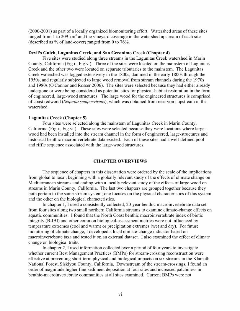
Devil's Gulch, Lagunitas Creek, and San Geronimo Creek (Chapter 4) Five sites were studied along three streams in the Lagunitas Creek watershed in Marin

County, California (Fig i., Fig v.). Three of the sites were located on the mainstem of Lagunitas Creek and the other two were located on separate tributaries to the mainstem. The Lagunitas Creek watershed was logged extensively in the 1800s, dammed in the early 1800s through the 1950s, and regularly subjected to large wood removal from stream channels during the 1970s and 1980s (O'Connor and Rosser 2006). The sites were selected because they had either already undergone or were being considered as potential sites for physical-habitat restoration in the form of engineered, large-wood structures. The large wood for the engineered structures is comprised of coast redwood (Sequoia sempervirens), which was obtained from reservoirs upstream in the watershed.

Lagunitas Creek (Chapter 5) Four sites were selected along the mainstem of Lagunitas Creek in Marin County, California (Fig i., Fig vi.). These sites were selected because they were locations where large-wood had been installed into the stream channel in the form of engineered, large-structures and historical benthic macroinvertebrate data existed. Each of these sites had a well-defined pool and riffle sequence associated with the large-wood structures.

CHAPTER OVERVIEWS

The sequence of chapters in this dissertation were ordered by the scale of the implications from global to local, beginning with a globally relevant study of the effects of climate change on Mediterranean streams and ending with a locally relevant study of the effects of large wood on streams in Marin County, California. The last two chapters are grouped together because they both pertain to the same stream system; one focuses on the physical characteristics of this system and the other on the biological characteristics.

In chapter 1, I used a consistently collected, 20-year benthic macroinvertebrate data set from four sites along two small northern California streams to examine climate-change effects on aquatic communities. I found that the North Coast benthic macroinvertebrate index of biotic integrity (B-IBI) and other common biological-assessment metrics were not influenced by temperature extremes (cool and warm) or precipitation extremes (wet and dry). For future monitoring of climate change, I developed a local climate-change indicator based on macroinvertebrate taxa and tested it on an external dataset. I also examined the effect of climate change on biological traits.

In chapter 2, I used information collected over a period of four years to investigate whether current Best Management Practices (BMPs) for stream-crossing reconstruction were effective at preventing short-term physical and biological impacts on six streams in the Klamath National Forest, Siskiyou County, California. Downstream of the stream-crossings, I found an order of magnitude higher fine-sediment deposition at four sites and increased patchiness in benthic-macroinvertebrate communities at all sites examined. Current BMPs were not

vii

completely effective at preventing short-term, negative impacts on downstream habitats following stream-crossing reconstruction.

In chapter 3, I examined the effects of streamflow declines, associated with vineyard water withdrawals for frost protection, on benthic-macroinvertebrate communities at three sites along three streams in Napa and Sonoma counties. I also examined relationships between vineyard coverage and benthic-macroinvertebrate community response using data collected from 59 sites along 35 streams in Lake, Napa, and Sonoma Counties. I found that vineyard water withdrawals for frost protection coincided with declines in several biological metrics and that vineyard-coverage levels above a ~20% threshold coincided with effects on both biological metrics and traits.

In chapter 4, I examined the distribution of large wood and the effects that it had on pool formation in five stream reaches in Marin County, California. I found that large wood in the bankfull channels, particularly those pieces with root-wads or those that were part of clusters, had a strong influence on pool formation and that stream reaches with large-wood additions in the form of engineered, wood structures had lower values of channel widths per pool than those without large-wood additions. The streams in this study generally had lower amounts of large wood and higher values of channel widths per pool than streams of comparable size in other regions of the western United States. In chapter 5, I examined the effects of large wood on benthic macroinvertebrates in the same stream system in Marin County, California. I found that the percentage of organisms in the shredder functional-feeding group was significantly higher in pools created by engineered, large-wood structures than in nearby riffles, and that the dominant shredders in pools were caddisflies, whereas the dominant shredders in riffles were stoneflies. Using several additional biological metrics, I observed statistically significant differences between pools and riffles, and between benthic macroinvertebrate communities sampled over time following the addition of large wood to the system. One biological metric indicated that the addition of large wood may result in a potential increase in water quality.

viii

Fig. i. Map showing the approximate locations in Northern California of the studies contained in the five chapters of this dissertation.

ix

Fig. ii. A photograph of Hunting Creek at one of the sites in the climate-change study (Chapter 1).

x

Fig. iii. A photograph of Upper Boulder Creek at one of the sites in the stream-crossing study (Chapter 2).

xi

Fig. iv. A photograph of Bidwell Creek at one of the sites in the vineyard study (Chapter 3).Photograph by Matthew J. Deitch, used with permission.

xii

Fig. vi. A photograph of Devils Gulch at one of the sites of the physical component of the large-wood study (Chapter 4).

xiii

Fig. vi. A photograph of Lagunitas Creek at one of the sites of the biological component of the large-wood study (Chapter 5).

xiv

Literature Cited

Barbour, M.T., Gerritsen, J., Snyder, B.D., and Stribling, J.B.1999. Rapid bioassessment protocols for use in streams and wadeable rivers: periphyton, menthic macroinvertebrates and fish, Second Edition. EPA 841-B-99-002. U.S. Environmental Protection Agency; Office of Water; Washington, D.C.

Barbour, M.T., and Stribling, J.B. 1991. Use of habitat assessment in evaluating the biological integrity of stream communities. In: G. Gibson (Ed.) Biological Criteria: Research and Regulation, pp. 25–38. Proceedings of a symposium, 12–13 December 1990, Arlington, Virginia. EPA-440-5-91-005. Office of Water, US Environmental Protection Agency, Washington, DC.

Barlow, M. and Clarke, 2002. T. Blue gold: the fight to stop the corporate theft of the world's water. New York Press, N.Y. ISBN: 1-5684-813-6.

Carter, J.L., Resh, V.H., Hannaford, M.J., and Myers, M.J. 2006. Macroinvertebrates as biotic indicators of environmental quality, p. 805-834. In: F.R. Hauer and G.A. Lamberti (eds.) Methods in Stream Ecology, 2nd Edition. Academic Press, Burlington, M.A.

Degerman, E., Beier U., Breine, J., Melcher, A., Quataert, P., Rogers, C., Roset, N., and Simnoens, I. 2007. Classification and assessment of degradation in European running waters. Fisheries Management and Ecology 14: 417-426.

Deitch, M.J. 2006. Scientific and institutional complexities of managing surface water for beneficial human and ecosystem uses under a seasonally variable flow regime in Mediterranean-climate Northern California. Dissertation. University of California, Berkeley. 323 pp.

Dunbar, M.J., Pedersen, M.K., Cadman, D., Extence, C., Waddingham, J., Chadd, R., and Larsen, S.E. 2010. River discharge and local-scale physical habitat influence macroinvertebrate LIFE scores. Freshwater Biology 55: 226-242.

Fritzmann, C., Löwenberg, J., Wintgens, T., and Melin, T. 2007. State-of-the-art of reverse osmosis desalination. Desalination 216: 1-76.

Guardiola, J., González-Gómez, F., Grajales, A.L. 2010. Is access to water as good as the data claim? Case Study of Yucatan. Water Resources Development 26: 219-233.

Hannaford, M.J., Barbour, M.T., and Resh, V.H. 1997. Training reduces observer variability in visual-based assessments of stream habitat. Journal of the North American Benthological Society 16: 853-860.

Harrelson, C.C, Rawlins, C.L., Potyondy, J.P. 1994. Stream channel reference sites: an illustrated guide to field technique. Gen. Tech. Rep. RM-245. Fort Collins, CO: U.S. Department of Agriculture, Forest Service, Rocky Mountain Forest and Range Experiment Station. 61 pp.

xv

Kaufmann, P.R., Levine, P., Robison, E.G., Seeliger, C. and Peck, D.V. 1999. Quantifying physical habitat in wadeable streams. EPA/610/R-99/003. U.S. Environmental Protection Agency, Washington, D.C.

Kondolf, G.M. 1997. Hungry water: effects of dams and gravel mining on river channels. Environmental Management 21: 533-551.

Morse, J.C., Bae, Y.J., Munkhjargal, G., Sangpradub, N., Tanida, K., Vshivkova, T.S., Wang, B., Yang, L., Yule, C.M. 2007. Freshwater biomonitoring with macroinvertebrates in East Asia. Frontiers in Ecology and the Environment 5: 33-42.

Poff, N.L., Olden, J.D., Merritt, D.M., and Pepin., D.M. 2007. Homogenization of regional river dynamics by dams and global biodiversity implications. PNAS 104: 5732-5737.

Purcell, A.H., Friedrich, C., Resh, V.H. 2002. An assessment of a small urban stream restoration project in Northern California. Restoration Ecology 10: 685-694.

Resh, V.H. 2008. Which group is best? Attributes of different biological assemblages used in freshwater biomonitoring programs. Earth and Environmental Science 138: 1-3.

Richter, B.D., Matthews, R., Harrison, D.L., and Wigington, R. 2003. Ecologically sustainable water management: managing river flows for ecological integrity. Ecological Applications 13: 206-224.

Risso, D.A. 2007. Floodplain vegetation following over 80 years of intensive land use and de-watering: Lower Owens River, California. M.S. Thesis. Oregon State University.

Rosenberg, D.M. and Resh, V.H. 1993. Introduction to freshwater biomonitoring and benthic macroinvertebrates, p. 1-9. In: D.M. Rosenberg and V.H. Resh (eds.) Freshwater biomonitoring and benthic macroinvertebrates. Chapman and Hall, N.Y.

Tanaka, S.K., Zhu, T., Lund, J.R., Howitt, R.E., Jenkins, M.W., Pulido, M.A., Tauber, M., Ritzema, R.S., and Ferreira, I.C. 2006. Climate warming and water management adaptation for California. Climate Change 76: 361-387.

CHAPTER 1

Long-term macroinvertebrate responses to climate change: implications for biological assessment in mediterranean-climate streams

1

Long-term macroinvertebrate responses to climate change: implications for biological assessment in mediterranean-climate streams

Abstract

Climate change is expected to have strong effects on mediterranean-climate regions worldwide. In some areas, these effects will include increases in temperature and decreases in rainfall, which could have important implications for biological assessment programs of aquatic ecosystems. I used a consistently collected, 20-year benthic macroinvertebrate data set from four sites along two small Northern California streams to examine potential climate-change effects on aquatic communities. The sites represented unique combinations of stream order and flow intermittency. The North Coast benthic macroinvertebrate index of biotic integrity (B-IBI) developed for northern California streams was not influenced by temperature extremes (cool and warm) or precipitation extremes (wet and dry). Other common indices and metrics used in biological monitoring studies, such as the ratio of observed to expected taxa (O/E), % Ephemeroptera, Plecoptera, and Trichoptera (EPT) individuals, and total richness were unaffected by temperature and precipitation variability. For future monitoring of climate-change effects on small streams, I developed a local climate-change indicator that is composed of the presence/absence of nine macroinvertebrate taxa, identified to genus level. This indicator detected significant differences between years that were grouped based on temperature, precipitation, and a combination of temperature and precipitation. It also detected significant differences between groups in an external data set including 40 reference sites throughout the San Francisco Bay area, a result that suggests this indicator could be used at larger spatial scales in this region. Two biological trait categories found in large, long-lived organisms decreased with increasing temperature and decreasing precipitation at the most intermittent site. This result indicates that climate change might selectively affect taxa with certain traits. The robustness of the North Coast B-IBI and other common indices and metrics to temperature and precipitation variability demonstrates their continued applicability for examining water quality under future climate-change scenarios, but suggests that they probably will not be good indicators for detecting climate-change effects. The effects of climate change in mediterranean-climate streams can be monitored effectively within the framework of existing biological assessment programs by using regional indicators based on specific taxa identified to the generic level and information on their species traits.

Key words: climate change, mediterranean streams, benthic macroinvertebrates, biological assessment, climate indicators, B-IBI, species traits.

2

Introduction

Long-term studies, particularly studies that span greater than 10 years, are still relatively rare in freshwater ecology (Jackson and Füreder 2006), even though a long-term perspective is essential to understanding actual and potential impacts of climate change on community composition and structure in aquatic systems. Studies that span >10 years are particularly useful when examining the effects of long-term fluctuations in hydrology or temperature on macroinvertebrate communities (e.g., Bradt et al. 1999, Daufresne et al. 2004, Bêche and Resh 2007a, Ormerod and Durance 2009). Long-term studies also have established links between changes in macroinvertebrate communities and extreme climatic events (e.g., drought: Mouthon and Daufresne 2006, Bêche et al. 2009; freezing: Mulholland et al. 2009) and climatic cycles (North Atlantic Oscillation [NAO]: Bradley and Ormerod 2001, and El Niño Southern Oscillation [ENSO]: Bêche and Resh 2007b, Gilbert et al. 2008), both of which might increase in frequency under climate change (IPCC 2008). Several studies from European temperate regions have demonstrated directional trends in community structure associated with increasing temperatures or climate-change-related shifts in stream flow (Daufresne et al. 2004, 2009, Burgmer et al. 2007, Durance and Ormerod 2007, 2009, Chessman 2009, Ormerod and Durance 2009). These shifts in community composition and structure are largely a result of selection toward temperature- or low-flow-tolerant species (Chessman 2009). Research examining the effects of climate change on species traits has focused primarily on individual taxonomic groups rather than entire communities (Mouthon and Daufresne 2006, Cordellier and Pfenninger 2008, Spooner and Vaughn 2008, Clausnitzer et al. 2009, Hering et al. 2009, Stamp et al. 2010). However, evidence exists that aquatic communities could experience dramatic shifts toward smaller size distributions with climate change, a pattern that has been shown for freshwater fishes and phytoplankton (Daufresne et al. 2009). This information brings into question the long-term applicability of newly established monitoring programs for local effects (e.g., urbanization and agriculture) because the metrics for reference sites (e.g., biotic indices) might be affected by climate change (Hamilton et al. 2010, Nichols et al. 2010). However, evidence from studies conducted in Europe suggests that biotic indices will be robust in the face of climate change, in that they will continue to be useful for detecting effects of the types of water pollution for which they were designed (Zamora-Muñoz et al. 1995, Morais et al. 2004, Leunda et al. 2009). The implications of climate-change effects are region-specific in that the existing climate and the characteristics of its communities influence the potential responses to climate change (e.g., arctic ecosystems, Heino et al. 2009). Most climate-change research has been focused on temperate ecosystems, particularly in Europe (Rosenzweig et al. 2008), and research on aquatic macroinvertebrates is no exception to this pattern. In particular, little research has been done on potential climate-change effects in aquatic ecosystems in mediterranean-climate regions (MCRs). Bêche and Resh (2007a, b) and Bonada et al. (2007) have conducted studies suggesting that climate change might lead to greater changes in taxonomic composition than in biological traits (e.g., life-history traits and size) in MCRs. However, few studies have explicitly examined the effects of climate change (e.g., temperature increase) on benthic macroinvertebrates in these climatic

3

regions (but see Feio et al. 2010). Temperature and precipitation extremes over the past 20 years in the MCR of

California have been analyzed using a range of time-series analyses. These extremes were determined, with high statistical confidence, to be outside of the range of natural variability (Bonfils et al. 2007, Maurer et al. 2007). Air temperatures in this region are expected to increase, on average, by an additional 1.5 to 4.5°C by 2100 (Cayan et al. 2009). Expectations for precipitation are more variable among existing models, but a drying tendency is expected in some locations (Cayan et al. 2009). Most General Circulation Models (GCMs) for California project greater warming in summer than in winter, most annual precipitation to continue to occur in winter, and possibly a longer rainy season with more sporadic individual rainfall events (Cayan et al. 2009). Most GCMs indicate that California will retain its characteristic mediterranean climate with relatively cool, wet winters and hot, dry summers.

Benthic macroinvertebrates are sensitive to changes in temperature, precipitation, and the associated flow regimes (Bunn and Arthington 2002, Lytle and Poff 2004), which should make them particularly responsive to the effects of climate change. For example, the anticipated increases in regional air temperatures, and consequently, water temperatures, which are closely related to air temperatures in small streams (Caissie 2006, Nelson and Palmer 2007), probably will affect benthic macroinvertebrates in MCR streams because temperature affects growth and timing of development and emergence (Bayoh and Lindsay 2003). Seasonal differences (rainy vs dry) in the abundance and composition of benthic macroinvertebrates in the MCR of California diminished during drought years and were correlated with patterns in ENSO, which are linked to temperature and precipitation (Bêche and Resh 2007b, Mazor et al. 2009). No evidence exists that the frequency or intensity of ENSO will increase because of climate change, but most GCMs indicate that ENSO will continue to influence climate patterns over the next century (Cayan et al. 2009). In addition, some metrics (e.g., taxon richness and Ephemeroptera, Plecoptera, Trichoptera [EPT] richness) are highly variable among years in coastal California streams, whereas others (e.g., Benthic Index of Biotic Integrity [B-IBI] and the ratio of observed to expected taxa [O/E] scores) are less variable (Mazor et al. 2009). The effects of climate change on these metrics and indices, on specific taxa, and on species traits have not been examined in detail in other studies. My objectives were to determine: 1) whether the core multimetric indicator of biological assessment programs in northern California (North Coast B-IBI; Rehn et al. 2005) will be robust against temperature and precipitation patterns associated with climate change, 2) whether commonly used metrics and indices are responsive to temperature and precipitation change (e.g., % EPT individuals, O/E scores); 3) whether taxon-based indicators that respond to climate change can be developed; and 4) whether a priori selected biological traits are responsive to climate change. These objectives have important implications for evaluating local landuse effects with biological monitoring programs in California because these programs are based on reference conditions, which might be affected by climate change. If so, multimetric indicators might have to be adjusted, e.g., by removing metrics sensitive to climate change, to detect reliably disturbances associated with land use. These implications of climate change also might be relevant to biological assessment programs in other MCRs, including areas in parts of Europe, southern California, South Africa, Australia, and Chile (Gasith and Resh 1999).

4

Methods

Study site and existing data This study is based on a 20-year, consistently collected benthic macroinvertebrate data set. Studies based on data sets of comparable duration have made important contributions to our understanding of climate-change effects (e.g., Perry et al. 2005, Both et al. 2006, Rosenzweig et al. 2008). This data set might be particularly valuable because its length is comparable to most existing biological monitoring programs in the US (Resh and Rosenberg 1989, Jackson and Füreder 2006). Thus, the findings might apply directly to these programs. This data set also is one of the most consistent data sets collected, in that benthic macroinvertebrates were sampled each year by the same individual (V. Resh), and identifications were done by the same individual (E. McElravy). Each collection consisted of 5 Surber samples (0.093 m2, 500-μm mesh), and all individuals in each sample were identified to genus or species (see Bêche et al. 2006 for additional detail).

The data set is composed of collections from four sites along two small, first- and second- order, northern California streams, Knoxville and Hunting Creeks, in Lake County and Napa County, California (Fig. 1.1). The watersheds are relatively unaltered and are considered to represent reference conditions for small streams in the northern California MCR (see Bêche and Resh 2007a, b and Mazor et al. 2009 for further site details). Modest evidence exists that the benthic macroinvertebrate communities at the sites are relatively independent of each other and that the communities at the individual sites are correlated in time (Bêche and Resh 2007a, b). Sampling was done annually near 15 April from 1984 to 2003 at three of the sites (sites 1D, 2D, 2P), and from 1985 to 2003 at one of the sites (site 1P). The sampling date represents the end of the wet season, when most preemergence growth in all benthic macroinvertebrate orders occurs in this region (Mendez and Resh 2008). Samples were collected in a random design, stratified within riffles, and the same riffles were sampled each year. Two of the sampling sites are characterized by nonperennial flow (1D, 2D), and two are characterized by perennial flow (1P, 2P). Watershed areas range from ~2 to ~29 km2, and the sites are all within a 500-m elevation range (Table 1.1).

Temperature and precipitation Daily air temperature records were obtained from the meteorological station near

Knoxville Creek within the University of California McLaughlin Nature Reserve (Fig. 1). These daily air temperature records covered the entire duration of the study except for the first year and some short gaps over the remaining years (<23 days). To create a complete daily data set for the study duration, daily air temperatures at Knoxville Creek were plotted against those at Napa State Hospital, which is ~60 km south of the study sites, and any missing values were calculated with the equation determined from a linear regression between the data from these two stations. Daily air temperature records were used to calculate degree days (dd), which are correlated with insect development (Wilson and Barnett 1983). A threshold air temperature of 10°C was used as a baseline for calculating degree days because it is within the range of many macroinvertebrate species (Corkum 1992). The threshold temperature is the lower limit for invertebrate growth and development. A uniform value

5

of the threshold temperature was used because our goal was only to distinguish warm years from cold years from the perspective of invertebrate development and not to elucidate distinct differences among the many aquatic species collected. The number of days that exceeded this threshold was calculated over the 15-week period (January 1 to April 15) leading up to the sampling date. Daily precipitation records were obtained from Napa State Hospital for the duration of the study. Complete records were unavailable from the closer meteorological station operated at the McLaughlin Reserve. The total amount of precipitation that occurred over the 15-week period leading up to the sampling date was calculated to create a precipitation variable for analysis. To maintain consistency with the temperature analysis, the analysis was limited to the calendar year rather than to the start of the wet season in California, which typically occurs in October to early November, or to the water year, which begins October 1. The use of the calendar year is justified because new colonization of benthic macroinvertebrates is likely to occur throughout the duration of the wet season. Thus, starting at the beginning of the wet season is not crucial. Furthermore, years that are wetter on average in October through December tend to be wetter on average in January through April, and the same is true for temperature. The relationship between air temperature (dd) and precipitation was examined using linear regression. A correlation between air temperature and precipitation could indicate synergistic effects between these variables. For example, high air temperatures could lead to low flows, which could lead to higher local water temperatures because of less thermal mass. The years were ranked by number of degree days and by rainfall over the 15-week period leading up to the sampling date. These rankings were used to establish six groups, each consisting of the seven years at the extremes of the rankings: 1) cool vs warm, 2) wet vs dry, and 3) cool/wet vs warm/dry. Membership of years in groups was not exclusive (e.g., 1998 occurred in the cool group, the wet group, and the cool/wet group). The cool/wet and warm/dry groups were established by multiplying the rankings for temperature and precipitation to create a combined ranking that was used to sort years. The 20 years in this data set were particularly dry compared to the past 50 years (Bêche et al. 2009), but each group was distinct (Table 1.2). The average degree days in cool years (28) was significantly different from warm years (51) (p < 0.001), and the average total precipitation in wet years (53 mm) was significantly different from dry years (22 mm) (p < 0.001). Therefore, I judged that interannual variability that occurred during the study period would be informative. At the very least, analyzing climate variability in the past would underestimate future climate changes, which are expected to be more extreme than those that have already occurred (IPCC 2008). The third grouping, cool/wet vs warm/dry, was developed to determine if a synergistic effect between temperature and precipitation was evident in any of the metrics. Macroinvertebrate analyses

Collection data The data from the five benthic macroinvertebrate samples for each collection

event were combined by taking their average to avoid pseudoreplication in comparisons among sites. This composite data set was used to calculate a presence/absence matrix. Biological trait information was collected for nearly all of the taxa in the data set from a

6

variety of published sources (see Bêche et al. 2006, Bêche and Resh 2007b for methods). The data consisted of 206 taxa and 146,697 individuals comprising 79 families and 24 orders. However, converting these taxa to operational taxonomic units (OTUs) for metric calculation reduced the number of taxa to 137 OTUs. This reduction was primarily a result of aggregation of Chironomidae to family and elimination of semiaquatic Hemiptera. Converting these taxa for calculation of the O/E calculation further reduced the number to 125 OTUs for the O/E analyses.

Independence among sites was examined using nonmetric multidimensional scaling analysis (NMDS) on the log10(x + 1)-transformed taxon abundances of all taxa. PC-ORD 4.27 software (MjM Software Design, Gleneden Beach, Oregon) was used to obtain a two-dimensional solution based on Sørenson distance (McCune and Mefford 1999). Clustering among the sites in ordination space was examined in relation to the categorical variables, stream order, and perenniality. The NMDS was run with two axes, 10 runs with real data, a stability criterion of 0.006, 50 iterations to evaluate stability, and a maximum number of iterations of 100.

Biological metrics evaluated for robustness to climate change The North Coast B-IBI is a multimetric index developed for water-quality

monitoring in northern California (Rehn et al. 2005) and is used in California by state agencies to evaluate local anthropogenic stresses on stream communities (Rehn et al. 2007). The eight metrics that comprise the North Coast B-IBI are: EPT richness, Coleoptera richness, Diptera richness, % intolerant individuals, % nongastropod scraper individuals, % predators, % shredder taxa, and % noninsect taxa. These metrics were calculated from the data with a Monte Carlo simulation without replacement to standardize sample size to 500 individuals, as required by the North Coast B-IBI (Rehn et al. 2005). For each site, the response of these metrics to both degree days and total precipitation (for the 15-week period prior to sampling) was determined with linear regression. In addition, Student’s t-tests were used to compare the average North Coast B-IBI value between the a priori groupings (e.g., cool vs warm, wet vs dry, and cool/wet vs warm/dry) to determine whether the North Coast B-IBI could be used as an indicator of climate change for this locality.

Several other widely used indices and metrics were evaluated to determine if they were responsive to temperature and precipitation change: % EPT individuals, total richness, and EPT richness divided by Odonata, Coleoptera, Hemiptera richness (EPT/OCH; Bonada et al. 2006). The O/E(50) was calculated from a River Invertebrate Prediction and Classification System (RIVPACS)-type model developed for California (see Ode et al. 2008 for details). O/E(50) includes only the common species found at >50% of reference sites. Each metric and index was plotted against degree days and precipitation and fit with linear regression. Student’s t-tests were used to compare values for cool vs warm years, wet vs dry years, and cool/wet vs warm/dry years. A p-value of 0.2 was selected as a threshold of significance to reduce the probability of false negatives (Type II error) for marginally affected metrics. No metric was strongly affected. This analysis was primarily exploratory and was not intended to establish significance rigorously, so Bonferroni corrections were not made.

7

Local climate-change indicator The final climate-change indicator was based on annual presence/absence data

from the taxa observed at all four sites. Annual presence/absence gave equal weight to taxa that were less common. To construct the final indicator, individual temperature (warm vs cool) and precipitation (dry vs wet) indicators (hereafter, preliminary temperature and precipitation indicators) were developed from the data set with an iterative process that used only a random subset of the data. For example, the first iteration of the preliminary temperature indicator used six of the seven years that fit the warm and cool criteria, respectively. Within the warm group, six years of data at four sites yielded a total of 24 sampling events for screening. The year that was randomly withheld from the seven years in each group for each iteration was used for internal validation and for consideration of taxa for inclusion in the final climate-change indicator as discussed below. All taxa were screened to determine which were more common in the warm than in the cool group by greater than or equal to eight of 24 sampling events (a difference of 33%). For example, if a given taxon was present at 12 sampling events during the warm years of one iteration, and four sampling events during the cool years, it would be selected for inclusion in this iteration. The total number of taxa selected by this process was calculated for each iteration. For example, in the first iteration, 12 taxa showed a positive affinity with warm years. The next step was to determine the presence of these taxa at each individual site–year combination, which was recorded as the proportion present out of those 12. Thus, 24 different proportions/iteration were calculated from these six years of data (four sites/year). The mean and standard error of this proportion were calculated, and a t-test was used to compare the preliminary temperature indicator between warm years (8.2/12) and cool (3.3/12) years in the first-iteration example. Internal validation was completed simultaneously with the taxon-screening process. For example, in the first iteration for the cool vs warm comparison, the preliminary temperature indicator was composed of 12 taxa. The next step was to determine the presence of these taxa at each site in the data for the year that was withheld for internal validation. The proportion present of those 12 taxa was recorded. Therefore, four different proportions/iteration were calculated from this one year of validation data. A t-test was used to compare the preliminary temperature indicator between warm (7.3/12) and cool (7.8/12) years in our first iteration example. When the result was significant, the taxa in that iteration were each given a point and considered for the final indicator. The total number of significant comparisons among the iterations of this internal validation was compared against the total number of significant comparisons from the six years that were used to select the taxa to assess the validity of the approach. This iteration process was completed 10 times for the wet vs dry groups and 10 times for the cool vs warm groups. To determine which taxa to include in the final climate-change indicator, which represented a combination of temperature and precipitation effects, a criterion for taxa was set that resulted in significant t-tests between groups in the internal validation on greater than or equal to four of 20 possible comparisons (e.g., the taxa had greater than four points). For example, the caddisfly genus Hydroptilia, which was included in the final indicator, was involved in five of five significant temperature models and two of five significant precipitation models, and, therefore, was significant on seven occasions. The goal for selecting taxa from the

8

significant comparisons in the internal validation was to reduce the limitations of fitting the model to the specific years of the study. Last, the proportional value of the final climate-change indicator was transformed to a 10-point scale to make the indicator values easier to compare on a linear scale. An external validation was done on the final climate-change indicator to reduce the limitations of fitting the model to the specific sites of the study. This external validation was accomplished with a data set of 47 individual sampling events made at 40 reference sites from 2000 to 2007 across the greater San Francisco Bay area. Benthic macroinvertebrates in this data set were collected with a targeted-riffle sampling method (Barbour et al. 1999). Most sites were sampled by personnel from the San Francisco Regional Water Quality Control Board through the Surface Water Ambient Monitoring Program (SWAMP). Additional sites were sampled by personnel from the Alameda Countywide Clean Water Program, Contra Costa Clean Water Program, Marin County Stormwater Pollution Prevention Program, San Mateo Countywide Water Pollution Prevention Program, Santa Clara Valley Urban Runoff Pollution Prevention Program, Sonoma Ecology Center, and the Institute for Conservation Advocacy Research and Education. To test the indicator on the external data set, the two wettest years (2005, 2006) and two driest years (2001, 2007) were selected from this eight-year period. The mean and standard error of the climate-change indicator were calculated for each precipitation group (wet and dry) with the final taxa that were selected for the indicator from the 20-year study data set. These values were compared (wet vs dry years) with a t-test. If the values were significantly different, the external validation was deemed successful. Last, the value of the final climate-change indicator was calculated for the original groups containing seven years of data for each site (cool vs warm, wet vs dry, and cool/wet vs warm/dry). The mean and standard error were calculated for each group, and differences between groups were evaluated with a t-test.

Biological traitsThree biological traits (voltinism, maximum body size, and desiccation

resistance) were hypothesized a priori to be sensitive to temperature or precipitation based on their functional attributes (Bêche et al. 2006, Bonada et al. 2007). I focused on specific categories within these traits (semivoltine life cycle, maximum body size >40 mm, and desiccation resistance) that probably would respond to climate-change effects. The distribution of biological traits among taxa was calculated from the presence–absence matrix instead of the abundance data because some taxa with these traits tend to be rare in the community. The traits for all taxa present in each sample and the proportional representation of each trait category were determined. The fuzzy coding approach was used (Chevenet et al. 1994), so each taxon could be described by a fractional composition of multiple trait categories (where the fractions sum to 1), e.g., a taxon could be described as 0.4 semivoltine and 0.6 bivoltine, which would indicate that this taxon has partial semivoltine and partial bivoltine characteristics.

9

Results

Physical conditions The daily average air temperatures measured at Knoxville Creek were linearly related (R2 = 0.78) to those measured at Napa State Hospital (y = 1.3x – 4.5). Therefore, air temperatures and the degree days calculated for the sites were assumed to be comparable at each site. Degree days and precipitation from January 1 to April 15 were highly variable from year to year. Degree days ranged from a minimum of 14 in 1998 to a maximum of 66 in 1988, a five-fold difference. Precipitation ranged from 15 cm in 1988 to 68 cm in 1995 and 1998, also a five-fold difference. This high interannual variability is evident among the temperature and precipitation values characterizing the different year groups (Table 1.2). Degree days and precipitation were inversely related (R2 = 0.30, p = 0.01; Fig. 2) within the study area. Cool years were more likely to be wet, and warm years were more likely to be dry. This pattern explains the similarity in the years included in the cool and wet groups and in the years included in the dry and warm groups. However, the low R2

indicates that the effects of temperature and precipitation should not be treated as a single variable.

The NMDS plot revealed distinct clusters of first- and second-order sites (Fig. 1.3A) and of nonperennial and perennial sites (Fig. 1.3B). This result indicates that the benthic macroinvertebrate communities at each site were independent to some extent, despite being within the same watershed. The first axis on the NMDS plot was correlated with degree days (R2 = 0.22) and precipitation (R2 = 0.31). Degree days and precipitation were aligned in opposite directions, indicating a strong, negative correlation within ordination space (Fig. 1.3A, B).

Biological metrics The North Coast B-IBI did not change significantly with temperature and precipitation at any site (Fig. 1.4A–H). However, the low power of the test ( < 0.8 in each case) indicates a limited ability to detect a difference. Furthermore, the North Coast B-IBI did not differ significantly between cool and warm or wet and dry years (Table 1.3). The only significant (p 0.05) regressions among the eight component metrics of the North Coast B-IBI were Coleoptera richness against degree days at site 1P (Table 1.4), Coleoptera richness against precipitation at site 1D (Table 1.5), and % shredder taxa at site 1D (Table 1.5). In the regressions of metrics against degree days, Coleoptera richness, % intolerant individuals, % nongastropoda scraper individuals, and % noninsect taxa had regressions with p-values 0.2. In the regressions of metrics against precipitation, EPT richness, Coleoptera richness, % intolerant individuals, % predators, and % shredder taxa had regressions with p-values 0.2. Coleoptera richness and % intolerant individuals were correlated with both degree days and precipitation, results suggesting that these two metrics might be the most responsive to climate change. However, the direction of the Coleoptera richness responses differed between sites 1D and 2D. Most of the other indices and metrics were not responsive to temperature or precipitation fluctuations. The average values of O/E(50), % EPT individuals, and total richness showed no substantial trends with climate (Table 1.3). EPT/OCH showed the

10

greatest association with climate, but the direction was not consistent between wet and dry years.

Local climate-change indicatorDifferences in taxon occurrences between groups (warm vs cold and wet vs dry)

ranged from zero to 15 in most iterations and were close to zero for most of the 206 total taxa. A difference of greater than or equal to eight was the criterion for inclusion in the preliminary temperature and precipitation indicators. In the 20 iterations, the preliminary indicators detected a significant difference (p < 0.05) between groups (cool vs warm and wet vs dry) in all of the groups containing the six years of data from which the indicators were constructed. In these same 20 iterations, the preliminary indicators detected a significant difference between groups in half of the cool vs warm groups (iterations one, two, five, six, and ten) and half of the wet vs dry groups (iterations one, three, six, seven, and nine) that contained the one year of data withheld for internal validation purposes. Thus, internal validation indicated that this method adequately selected taxa 50% of the time. Of the 13 total genera selected as preliminary indicator taxa during the iterations (Table 1.6), nine were ultimately selected to comprise the final climate-change indicator because they were present in greater than three of the 20 iterations in the internal validation. The taxa that comprised the final indicator were Ambrysus (Hemiptera), Chironomidae (Diptera), Dixa (Diptera), Euparyphus (Diptera), Hydropsyche(Trichoptera), Hydroptilia (Trichoptera), Lepidostoma (Trichoptera), Ochrotrichia(Trichoptera), and Trichocorixa (Hemiptera). These taxa are in three orders: Trichoptera (n = 4), Diptera (n = 3), and Hemiptera (n = 2). Trichopterans made up 23% of the overall taxon list and 44% of the taxa in the indicator (i.e., four of the nine taxa selected), so it is unlikely that their high representation in the indicator is entirely the result of chance. The difference in the number of years of presence of these taxa between the cool and wet and the warm and dry groups ranged from five to 14 (Table 1.7).

The final climate-change indicator was able to detect a significant difference between year groups (warm vs cool, wet vs dry, cool/wet vs warm/dry) in 10 of the 12 comparisons examined (Table 1.8). The difference in the average indicator value for all the sites combined was highest between the dry and wet years (6.8 – 2.7 = 4.1). The difference between the cool and warm years and the cool/wet and warm/dry years was 2.8 in each case. This result agrees with the NMDS ordination (Fig. 1.3A, B) of the raw abundance data for all taxa, which showed that precipitation was a stronger driver than temperature in shaping patterns in the benthic community, as indicated by the length of the vector. The difference in the average indicator value between groups was typically larger in the nonperennial sites than in the perennial sites. The final climate-change indicator (developed with long-term data from four study sites in two streams) was robust when used with the external validation (regional) data set from 47 sampling events at 40 sites from throughout the greater San Francisco Bay area. The indicator values differed by 0.8 units between wet years (indicator value = 1.9) and dry years (indicator value = 2.8). This difference was smaller than that observed in the local data set (i.e., 2.8), but it was statistically significant (p = 0.001). All but one of the nine taxa were prevalent in both the local and regional data set. The exception was Ambrysus.

11

Biological traits Two of the three selected traits showed consistent trends between cool vs warm

years and wet vs dry years. However, these trends were statistically significant only at the site with the most extreme conditions of intermittency, i.e., the first-order, nonperennial (1D) site (Fig. 1.5A–D). The trends included a decrease in macroinvertebrates with a life cycle greater than one year and a decrease in macroinvertebrates with a body size greater than 40 mm with increasing temperature or with decreasing precipitation. Desiccation resistance, which was hypothesized to be potentially responsive to temperature, did not differ consistently or significantly among sites.

Cool/wet vs warm/dry years Metrics and indices did not differ more strongly between cool/wet years and warm/dry years, which represent the strongest combination of climate-change effects examined, than between wet and dry or cool and warm years. However, the difference in total richness between cool/wet years and warm/dry years was statistically significant at one of the sites (2P), whereas it was not significant for any of the individual temperature or precipitation comparisons (Table 1.3).

Discussion

The high interannual variability in temperature and precipitation that was observed among years in my study is characteristic of MCRs worldwide (Gasith and Resh 1999). This variability is related to the ENSO weather phenomenon through complex relationships that are region specific (Brönnimann et al. 2007). In the MCR of Europe, for example, the ENSO is nonlinearly associated with winter precipitation anomalies (Pozo-Vázquez et al. 2005). In the MCR of southern California, El Niño winters tend to be wetter than normal (Cayan et al. 2009), but the pattern is not as clear in northern California. Worldwide, the ENSO has played a key role in shaping patterns of climate variability in MCRs over the past millennium (Mann 2006). The significant inverse correlation between temperature and precipitation illustrates that the effects observed in my study could be related to either or both of these variables. Correlations between regional air temperatures and precipitation have been observed in other MCRs (e.g., Milly et al. 2005, Chu et al. 2008). However, the mechanism of influence from temperature might not be direct. For example, water temperature is inversely correlated with dissolved oxygen levels in streams and rivers, which can affect benthic macroinvertebrates (Morrill et al. 2005, Jacobsen and Marín 2007). In addition, the mechanism of the effect of dissolved oxygen on benthic macroinvertebrates could be related to other unmeasured explanatory variables, such as amount of canopy cover or groundwater input. These mechanisms could not be tested directly because year-to-year variability of these variables was not measured. The benthic macroinvertebrate communities observed in the perennial and nonperennial and in the first- and second-order sites were different, a result that is in agreement with the findings in Bêche and Resh (2007a, b), Bêche et al. (2009), and Mazor et al. (2009). Perenniality and stream order also shape distinct benthic communities in the MCRs of Europe (e.g., Bonada et al. 2007, Anna et al. 2009, Feio et al. 2010) and California (e.g., Bonada et al. 2006, Bêche et al. 2006, Bêche and Resh

12

2007b, Mazor et al. 2009). One of the key findings of this study was that the greatest association between biological traits and climate occurred in the first-order, nonperennial site 1D, probably because it represents the most extreme, intermittent conditions. The longer-lived (life cycle greater than one year), larger (maximum body size greater than 40 mm) organisms at this site were clearly less abundant in warmer and drier years, probably because of their lower tolerance to extreme conditions. Some of the most widely used biological metrics (e.g., % EPT, total richness) and local indices (e.g., the North Coast B-IBI) were robust against interannual changes in temperature and precipitation, so these metrics should have continued usefulness for biological assessment programs aimed at detecting local anthropogenic stressors under climate-change scenarios. However, the low power ( < 0.8) indicates that these findings should be interpreted cautiously. The values of the B-IBI and % EPT were low relative to values typically observed in reference sites in other parts of northern California outside the MCR. This difference is related to the stresses in the MCR, i.e., floods followed by drying, which are the reference conditions in this region. A fairly constant percent composition of the same dominant taxa was observed among the years, and this result indicates that the foundation of the benthic community might remain intact despite temperature and precipitation changes. This apparent resilience might be related to the unpolluted nature of these sites and to the severe conditions, i.e., sequential flooding and drying, of the mediterranean climate itself (Gasith and Resh 1999), which selects highly resilient organisms. For example, an unpolluted site would tend to have a higher EPT/OCH because of the higher EPT composition. However, an unpolluted site also could have low EPT/OCH if riffles are relatively less common than pools in the system (Bonada et al. 2006). EPT/OCH was lower in the warm than in the cold years at all sites and lower in the dry than in the wet years in three of the four sites although not all of these differences were statistically significant. A combination of polluted water and increasing temperature might have a compounded, negative effect on metrics based on the OCH orders, and this possibility should be tested further. The North Coast B-IBI and other commonly used metrics and indices might be unresponsive to the expected climate-change scenarios because many of the component metrics are calculated for taxa identified at the order level. Genera might come and go, but if replacement occurs, order-level metrics would be unchanged. However, some specific macroinvertebrate genera did appear to be consistently responsive to climate changes, and these taxa were the ones that we incorporated into the climate-change indicator. The functionality of the indicator might result from its ability to account for generic-level turnover, because it is based on individual taxa. These taxa, which were primarily trichopterans, might be among the most susceptible to climate change and could be useful components to include in biological-monitoring programs aimed at detecting climate-change effects. The debate about the general usefulness of higher (e.g., order and family) compared to lower (e.g., genus and species) levels of taxonomic resolution for evaluating anthropogenic changes has gone on for decades (e.g., Resh and Unzicker 1975). Lenat and Resh (2001) provide many examples of when species or generic levels might be more useful than higher levels. The potential usefulness of generic-level indicators for detecting climate change, which was a key finding of this study, suggests that this result should be added to that list.

13

Modest evidence was found for a filtering effect on biological traits at the site with the most extreme conditions of intermittency. This result indicates that the benthic communities in intermittent habitats might experience the strongest selective force under the expected conditions of climate change. This study also illustrates the usefulness of a priori hypothesis testing based on specific trait categories, which thus far, is not a widely used approach in trait studies on North American freshwater macroinvertebrates. The prevalence of specific biological traits (i.e., voltinism and maximum body size) differed significantly between cool and warm years and between wet and dry years at the most intermittent site, but any evolutionary response would occur over a much longer time period. Several studies conducted in MCRs have found that traits are less sensitive to climate change than are taxonomic composition and abundance measures (e.g., Bêche et al. 2006, Bêche and Resh 2007b, Bonada et al. 2007). However, the sensitivity of species traits might depend on the extremeness or severity of changes at a site, which tend to be highest in first-order, nonperennial streams and is compounded in streams without riparian cover. A presence-based, climate-change indicator appears to be useful for evaluating the effects of future climate change at the specific sites used in this study. Such an indicator also might be applicable at a regional scale, as evidenced by the successful external validation at sites throughout the San Francisco Bay area. However, the strength of the climate signal was lower between groups in the regional data set than in the local data set. The reduced signal strength in the region-wide application could be related to many unaccounted factors, including variability in sampling dates, local microclimates, food sources, and levels of endemism. In addition, site-level variability could have created additional noise in the analysis. An advantage of using a presence-based indicator rather than proportional metrics based on relative abundances is that presence-based indicators can be incorporated into rapid assessment protocols because all organisms in the samples need not be counted and identified. Likewise, because of the high correlation between degree days and precipitation, the reliability of the indicator is nearly the same whether it is used to detect change in temperature or precipitation. The strongest effects (i.e., difference between groups detected by the indicator) appear to result from precipitation, which indicates that flow regime might be the dominant driver of variability in the benthic community. The projection that climate change will result in regional temperature increases of one to five degrees Celsius in MCRs and the expectation that precipitation regimes will shift in a variety of ways among MCRs is well established (e.g., IPCC 2008, Cayan et al. 2009). Therefore, macroinvertebrate indicators like the one proposed here might be useful metrics for biological assessment programs that seek to monitor the effects of climate change. However, the effects of climate change might be more subtle than a single indicator alone can detect. This problem provides the incentive for obtaining additional information from measures based on selected biological traits. Small streams in MCRs, particularly first-order, nonperennial streams, might offer ideal conditions for monitoring climate change. Long-term studies are needed to develop effective indicators of climate change within specific ecoregions. Long-term monitoring and an understanding of species interactions are critical gaps in realistic predictions of the effects of climate change on benthic communities. Space-for-time substitutions are limited because of unaccounted site differences, which compound analytic difficulties.

14

However, this approach is often the only available choice. Museum collections of benthic macroinvertebrates might provide a useful source of long-term information about changes in benthic macroinvertebrate communities (e.g., Resh and Unzicker 1975, Hall and Ide 1987, DeWalt et al. 2005). Life-history studies also are useful for making decisions about climate change. Without these studies, no alternative sources of information can be used. Unfortunately, the decline in these studies might limit the use of species-traits-based analyses (Resh and Rosenberg 2010), an approach that already has proven effective in European MCRs.

Acknowledgements

I thank Peter Ode, Núria Bonada, Michael Barbour, and Pamela Silver for their detailed and insightful comments on this dissertation chapter. I also thank the US Department of Agriculture Forest Service under Cost Share Agreement #03-CR-11052007–042 and the Edward A. Colman Fellowship in Watershed Management from the Department of Environmental Science, Policy, and Management at the University of California, Berkeley, for support.

Literature Cited

Anna, A., C. Yorgos, P. Konstantinos, and L. Maria. 2009. Do intermittent and ephemeral Mediterranean rivers belong to the same river type? Aquatic Ecology 43: 465–476.

Barbour, M. T., J. Gerritsen, B. D. Snyder, and J. B. Stribling. 1999. Rapid bioassessment protocols for use in streams and wadeable rivers: periphyton, benthic macroinvertebrates and fish. 2nd edition. EPA 841-B-99-002. Office of Water, US Environmental Protection Agency, Washington, DC.

Bayoh, M. N., and S. W. Lindsay. 2003. Effect of temperature on the development of the aquatic stages of Anopheles gambiae sensu stricto (Diptera: Culicidae). Bulletin of Entomological Research 93: 375–381.

Bêche, L. A., P. G. Connors, V. H. Resh, and A. M. Merenlender. 2009. Resilience of fishes and invertebrates to prolonged drought in two California streams. Ecography 32: 779–788.

Bêche, L. A., E. P. McElravy, and V. H. Resh. 2006. Long-term seasonal variation in the biological traits of benthic macroinvertebrates in two mediterranean-climate streams. Freshwater Biology 51: 56–75.

Bêche, L. A., and V. H. Resh. 2007a. Biological traits of benthic macroinvertebrates in California mediterranean-climate streams: long-term annual variability and trait diversity patterns. Fundamental and Applied Limnology 161: 1–23.

15

Bêche, L. A., and V. H. Resh. 2007b. Short-term climatic trends affect the temporal variability of macroinvertebrates in California ‘mediterranean’ streams. Freshwater Biology 52: 2317–2339.

Bonada, N., S. Dolédec, and B. Statzner. 2007. Taxonomic and biological trait differences of stream macroinvertebrate communities between Mediterranean and temperate regions: implications for future climatic scenarios. Global Change Biology 13: 1658–1671.

Bonada, N., M. Rieradevall, N. Prat, and V. H. Resh. 2006. Benthic macroinvertebrate assemblages and macrohabitat connectivity in mediterranean-climate streams of northern California. Journal of the North American Benthological Society 25: 32–43.

Bonfils, C., P. B. Duffy, B. D. Santer, T. M. L. Wigley, D. B. Lobell, T. J. Phillips, and C. Doutriaux. 2007. Identification of external influences on temperatures in California. Climate Change 87: 43–55.

Both, C., S. Bouwhuis, C. M. Lessells, and M. E. Visser. 2006. Climate change and population declines in a long-distance migratory bird. Nature 441: 81–83.

Bradley, D. C., and S. J. Ormerod. 2001. Community persistence among stream invertebrates tracks the North Atlantic Oscillation. Journal of Animal Ecology 70: 987–996.

Bradt, P., M. Urban, N. Goodman, S. Bissell, and I. Spiegel. 1999. Stability and resilience in benthic macroinvertebrate assemblages. Hydrobiologia 403: 123–133.

Brönnimann, S., E. Xoplaki, C. Casty, A. Pauling, and J. Luterbacher. 2007. ENSO influence on Europe during the last centuries. Climate Dynamics 28: 181–197.

Bunn, S. E., and A. H. Arthington. 2002. Basic principles and ecological consequences or altered flow regimes for aquatic biodiversity. Environmental Management 30: 492–507.

Burgmer, T., H. Hillebrand, and M. Pfenninger. 2007. Effects of climate-driven temperature changes on the diversity of freshwater macroinvertebrates. Oecologia (Berlin) 151: 93–103.

Caissie, D. 2006. The thermal regime of rivers: a review. Freshwater Biology 51:1389–1406.

Cayan, D., M. Tyree, M. Dettinger, H. Hidalgo, T. Das, E. Maurer, P. Bromirski, N. Graham, and R. Flick. 2009. Climate change scenarios and sea level rise estimates for the California 2008 Climate Change Scenarios Assessment. CEC-500-2009-014-D. California Climate Change Center, Sacramento, California. (Available from: http://www.energy.ca.gov/2009publications/CEC-500-2009-014/CEC-500-2009-014-D.PDF)

16

Chessman, B. 2009. Climatic changes and 13-year trends in stream macroinvertebrate assemblages in New South Wales, Australia. Global Change Biology 15: 2791–2802.

Chevenet, F., S. Dolédec, and D. Chessel. 1994. A fuzzy coding approach for the analysis of long-term ecological data. Freshwater Biology 31: 295–309.

Chu, C., N. E. Jones, N. E. Mandrak, A. R. Piggott, and C. K. Minns. 2008. The influence of air temperature, groundwater discharge, and climate change on the thermal diversity of stream fishes in southern Ontario watersheds. Canadian Journal of Fisheries and Aquatic Sciences 65: 297–308.

Clausnitzer V., V. J. Kalkman, M. Ram, B. Collen, J. E. M. Baillie, M. Bedjani , W. R. T. Darwall, K. D. B. Dijkstra, R. Dow, J. Hawking, H. Karube, E. Malikova, D. Paulson, K. Schütte, F. Suhling, R. J. Villanueva, N. von Ellenrieder, and K. Wilson. 2009. Odonata enter the biodiversity crisis debate: the first global assessment of an insect group. Biological Conservation 142: 1864–1869.

Cordellier, M., and M. Pfenninger. 2008. Climate-driven range dynamics of the freshwater limpet, Ancylus fluviatilis (Pulmonata, Basommatophora). Journal of Biogeography 35: 1580–1592.

Corkum, L. D. 1992. Spatial distributional patterns of macroinvertebrates along rivers within and among biomes. Hydrobiologia 239: 101–114.

Daufresne, M., K. Lengfellner, and U. Sommer. 2009. Global warming benefits the small in aquatic ecosystems. Proceedings of the National Academy of Sciences of the United States of America 106: 12788–12793.

Daufresne, M., M. C. Roger, H. Capra, and N. Lamouroux. 2004. Long-term changes within the invertebrate and fish communities of the Upper Rhône River: effects of climatic factors. Global Change Biology 10: 124–140. DeWalt, R. E., C. Favret, and D. W. Webb. 2005. Just how imperiled are aquatic insects? A case study of stoneflies (Plecoptera) in Illinois. Annals of the Entomological Society of America 98: 941–950.

Durance, I., and S. J. Ormerod. 2007. Effects of climatic variation on upland stream invertebrates over a 25 year period. Global Change Biology 13: 942–957.

Durance, I., and S. J. Ormerod. 2009. Trends in water quality and discharge confound long-term warming effects on river macroinvertebrates. Freshwater Biology 54: 388–405.

Feio, M. J., N. C. Coimbra, M. A. S. Graça, S. J. Nichols, and R. H. Norris. 2010. The influence of extreme climatic events and human disturbance on macroinvertebrate community patterns of a Mediterranean stream, over 15 y. Journal of the North American Benthological Society 29: 000–000.

17

Gasith, A., and V. H. Resh. 1999. Streams in Mediterranean climate regions: abiotic influences and biotic responses to predictable seasonal events. Annual Review of Ecology and Systematics 30: 51–81.

Gilbert, B., P. J. Dillon, K. M. Somers, R. A. Reid, and L. Scott. 2008. Response of benthic macroinvertebrate communities to El Niño related drought events in six upland streams in south-central Ontario. Canadian Journal of Fisheries and Aquatic Sciences 65: 890–905.

Hall, R. J., and F. P. Ide. 1987. Evidence of acidification effects on stream insect communities in central Ontario between 1937 and 1985. Canadian Journal of Fisheries and Aquatic Sciences 44: 1652–1657.

Hamilton, A., J. D. Stamp, and B. Bierwagen. 2010. Vulnerability of biological metrics and multimetric indices to effects of climate change. Journal of the North American Benthological Society 29: 000–000.

Heino, J., R. Virkkala, and H. Toivonen. 2009. Climate change and freshwater biodiversity: detected patterns, future trends and adaptations in northern regions. Biological Reviews 84: 39–54.

Hering, D., A. Schmidt-Kloiber, J. Murphy, S. Lücke, C. Zamora-Muñoz, M. J. López-Rodríguez, T. Huber, and W. Graf. 2009. Potential impact of climate change on aquatic insects: a sensitivity analysis for European caddisflies (Trichoptera) based on distribution patterns and ecological preferences. Aquatic Sciences – Research Across Boundaries 71: 3–14.

IPCC (Intergovernmental Panel on Climate Change). 2008. Climate change and water. B. C. Bates, Z. W. Kundzewicz, S. Wu, and J. P. Palutikof (editors). Technical Paper of the Intergovernmental Panel on Climate Change Technical Paper IV. IPCC Secretariat, Geneva, Switzerland. (Available from: http://www.ipcc.ch/pdf/technical-papers/climate-change-water-en.pdf)

Jackson, J. K., and L. Füreder. 2006. Long term studies of freshwater macroinvertebrates: a review of the frequency, duration, and ecological significance. Freshwater Biology 51: 591–603.

Jacobsen, D., and R. Marín. 2007. Bolivian Altiplano streams with low richness of macroinvertebrates and large diel fluctuations in temperature and dissolved oxygen. Aquatic Ecology 42: 643–656.

Lenat, D. R., and V. H. Resh. 2001. Taxonomy and stream ecology: the benefits of genus- and species-level identifications. Journal of the North American Benthological Society 20: 287–298.

18

Leunda, P. M., J. Oscoz, R. Miranda, and A. H. Ariño. 2009. Longitudinal and seasonal variation of the benthic macroinvertebrate community and biotic indices in an undisturbed Pyrenean river. Ecological Indicators 9: 52–63.

Lytle, D. A., and N. L. Poff. 2004. Adaptation to natural flow regimes. Trends in Ecology and Evolution 19: 94–100.

Mann, M. E. 2006. Climate changes over the past millennium: relationships with Mediterranean climates. Il Nuovo Cimento 29: 73–80.

Maurer, E. P., I. T. Stewart, C. Bonfils, P. B. Duffy, and D. Cayan. 2007. Detection, attribution, and sensitivity of trends toward earlier streamflow in the Sierra Nevada. Journal of Geophysical Research-Atmospheres 112: D11118. doi:10.1029/2006JD008088

Mazor, R. D., A. H. Purcell, and V. H. Resh. 2009. Long-term variability in bioassessments: a twenty-year study from two Northern California streams. Environmental Management 43: 1269–1286.

McCune, B., and M. J. Mefford. 1999. PC-ORD: multivariate analysis of ecological data. Version 4.27. MjM Software, Gleneden Beach, Oregon.

Mendez, P. K., and V. H. Resh. 2008. Life history of Neophylax richeri (Trichoptera: Uenoidae) in two Northern California streams. Annals of the Entomological Society of America 101: 573–584.

Milly, P. C. D., K. A. Dunne, and A. V. Vecchia. 2005. Global pattern of trends in streamflow and water availability in a changing climate. Nature 438: 347–350.

Morais, M., P. Pinto, P. Guilherme, J. Rosado, and I. Antunes. 2004. Assessment of temporary streams: the robustness of metric and multimetric indices under different hydrological conditions. Hydrobiologia 516: 229–249.

Morrill, J. C., R. C. Bales, and M. H. Conklin. 2005. Estimating stream temperature from air temperature. Journal of Environmental Engineering 131: 139–146.

Mouthon, J., and M. Daufresne. 2006. Effects of the 2003 heatwave and climatic warming on mollusc communities of the Saône: a large lowland river and of its two main tributaries (France). Global Change Biology 12: 441–449.

Mulholland, P. J., B. J. Roberts, W. R. Hill, and J. G. Smith. 2009. Stream ecosystem responses to the 2007 spring freeze in the southeastern United States: unexpected effects of climate change. Global Change Biology 15: 1767–1776.

Nelson, K. C., and M. A. Palmer. 2007. Stream temperature surges under urbanization and climate change: data, models, and responses. Journal of the American Water Resources Association 43: 440–452.

19

Nichols, S. J., W. A. Robinson, and R. H. Norris. 2010. Using the reference condition maintains the integrity of a bioassessment program in a changing climate. Journal of the North American Benthological Society 29: 000–000. Ode, P. R., C. P. Hawkins, and R. D. Mazor. 2008. Comparability of biological assessments derived from predictive models and multimetric indices of increasing geographic scope. Journal of the North American Benthological Society 27: 967–985.

Ormerod, S. J., and I. Durance. 2009. Restoration and recovery from acidification in upland Welsh streams over 25 years. Journal of Applied Ecology 46: 164–174.

Perry, A. L., P. J. Low, J. R. Ellis, and J. D. Reynolds. 2005. Climate change and distribution shifts in marine fishes. Science 308: 1912–1915.

Pozo-Vázquez, D., S. R. Gámiz-Fortis, J. Tovar-Pescador, M. J. Esteban-Parra, and Y. Castro-Díez. 2005. El Niño-Southern Oscillation events and associated European winter precipitation anomalies. International Journal of Climatology 25: 17–31.

Rehn, A. C., P. R. Ode, and C. P. Hawkins. 2007. Comparisons of targeted-riffle and reach-wide benthic macroinvertebrate samples: implications for data sharing in stream-condition assessments. Journal of the North American Benthological Society 26: 332–348.

Rehn, A. C., P. R. Ode, and J. T. May. 2005. Development of a benthic index of biotic integrity (B-IBI) for wadeable streams in northern coastal California and its application to regional 305(b) reporting. Unpublished technical report for the California State Water Quality Control Board, Sacramento, California. (Available from: http://www.swrcb.ca.gov/water_issues/programs/swamp/reports.shtml)

Resh, V. H., and D. M. Rosenberg. 1989. Spatial-temporal variability and the study of aquatic insects. Canadian Entomologist 121: 941–963.

Resh, V. H., and D. M. Rosenberg. 2010. Recent trends in life-history research on benthic macroinvertebrates. Journal of the North American Benthological Society 29: 207–219.

Resh, V. H., and J. D. Unzicker. 1975. Water quality monitoring and aquatic organisms: the importance of species identification. Journal of the Water Pollution Control Federation 47: 9–19.

Rosenzweig, C., D. Karoly, M. Vicarelli, P. Neofotis, Q. Wu, G. Casassa, A. Menzel, T. L. Root, N. Estrella, B. Seguin, P. Tryjanowski, C. Liu, S. Rawlins, and A. Imeson. 2008. Attributing physical and biological impacts to anthropogenic climate change. Nature 453: 353–357.

20

Spooner, D. E., and C. C. Vaughn. 2008. A trait-based approach to species’ roles in stream ecosystems: climate change, community structure, and material cycling. Oecologia (Berlin) 158: 307–317.

Stamp, J. D., A. Hamilton, L. Zheng, and E. W. Leppo. 2010. Use of thermal preference metrics to examine state biomonitoring data for climate change effects. Journal of the North American Benthological Society 29: 000–000.

Wilson, L. T., and W. W. Barnett. 1983. Degree-days: an aid in crop and pest management. California Agriculture 37: 4–7.

Zamora-Muñoz, C., Sáinz-Cantero, C. E., Sánchez-Ortega, A., and J. Alba-Tercedor. 1995. Are biological indices BMPW' and ASPT' and their significance regarding water quality seasonally dependent? Factors explaining their variations. Water Research 29: 285–290.

21

Fig. 1.1. Site map showing streams as black lines. Site 1D is on Hunting Creek, and sites 1P, 2P, and 2D are on Knoxville Creek.

22

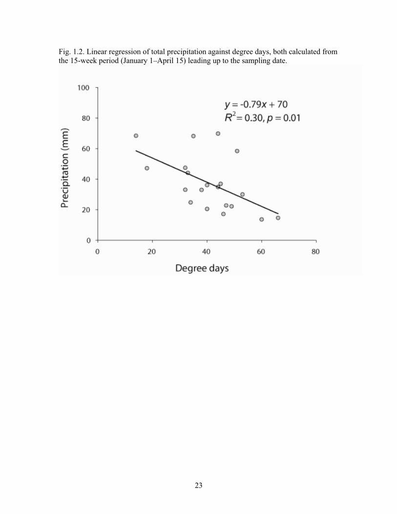
Fig. 1.2. Linear regression of total precipitation against degree days, both calculated from the 15-week period (January 1–April 15) leading up to the sampling date.

23

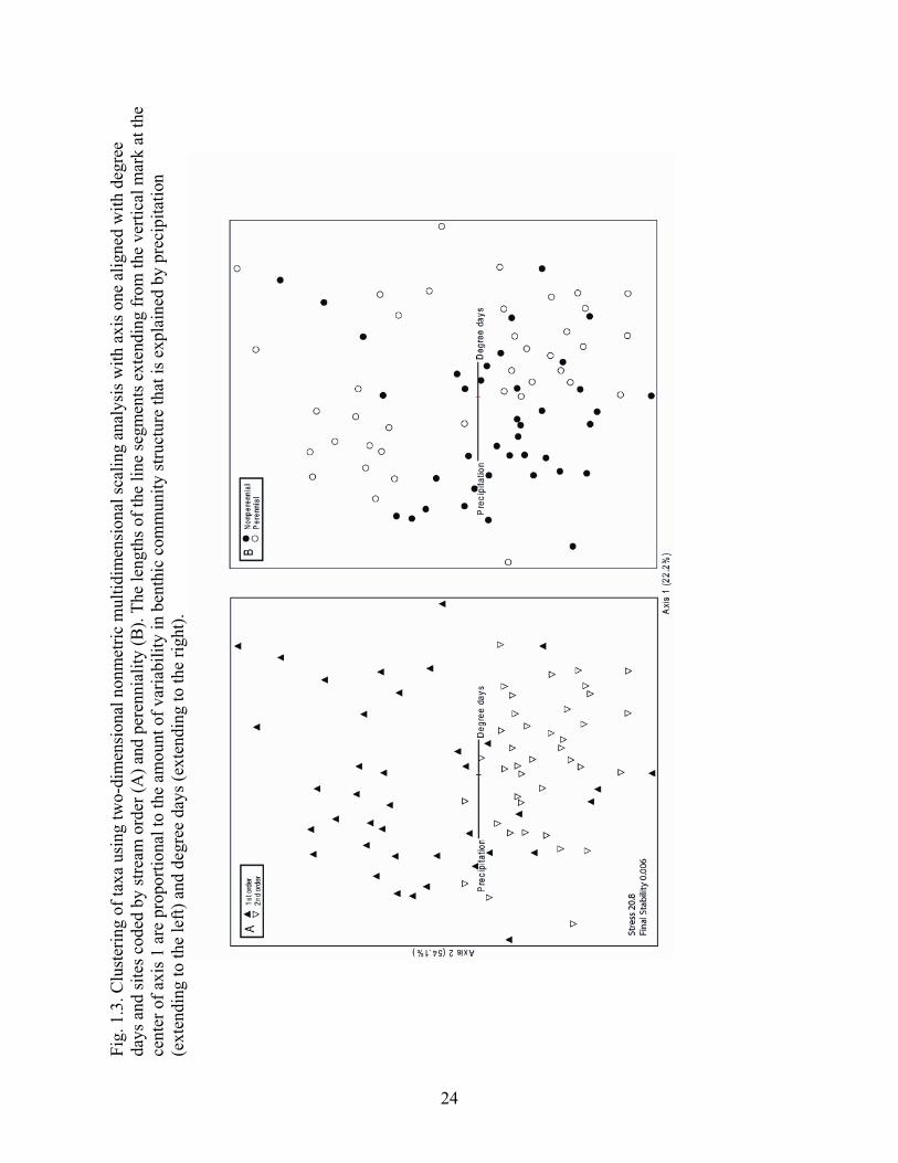
Fig.

1.3

. Clu

ster

ing

of ta

xa u

sing

two-

dim

ensi

onal

non

met

ric m

ultid

imen

sion

al sc

alin

g an

alys

is w

ith a

xis o

ne a

ligne

d w

ith d

egre

eda

ys a

nd si

tes c

oded

by

stre

am o

rder

(A) a

nd p

eren

nial

ity (B

). Th

e le

ngth

s of t

he li

ne se

gmen

ts e

xten

ding

from

the

verti

cal m

ark

at th

e ce

nter

of a

xis 1

are

pro

porti

onal

to th

e am

ount

of v

aria

bilit

y in

ben

thic

com

mun

ity st

ruct

ure

that

is e

xpla

ined

by

prec

ipita

tion

(ext

endi

ng to

the

left)

and

deg

ree

days

(ext

endi

ng to

the

right

).

24

Fig.

1.4

. The

Nor

th C

oast

Ben

thic

Inde

x of

Bio

tic In

tegr

ity (B

-IB

I) p

lotte

d ag

ains

t deg

ree

days

and

pre

cipi

tatio

n at

site

s 1D

(A, E

), 2D

(B

, F),

1P (C

, G),

and

2P (D

, H) a

nd fi

t with

line

ar re

gres

sion

tren

d lin

es.

25

Fig. 1.5. Mean (±1 SE) proportion of taxa with semivoltine life cycles (A, C) and maximum body size >40 mm (B, D) at the study sites in cool and warm years (A, B) and wet and dry years (C, D). * indicates a significant difference ( = 0.05) between groups of years (Student’s t-test).

26

Tabl

e 1.

1. P

hysi

cal c

hara

cter

istic

s of t

he st

udy

site

s.

Site

St

ream

St

ream

or

der

Pere

nnia

lity

Wat

ersh

ed a

rea

(km

2 )La

titud

e (N

) Lo

ngitu

de

(W)

Elev

atio

n(m

) St

ream

wid

th

(m)

1D

Kno

xvill

e C

reek

1

Non

pere

nnia

l 2.

1 38

°47'

56"

122°

18'5

3"

390

3–8

2D

Hun

ting

Cre

ek

2 N

onpe

renn

ial

22.1

38

°48'

30"

122°

22'4

5"

402

10–1

5 1P

H

untin

g C

reek

1

Pere

nnia

l 4.

4 38

°51'

56"

122°

24'5

4"

634

5–10

2P

H

untin

g C

reek

2

Pere

nnia

l 29

.3

38°4

9'45

" 12

2°22

'36"

34

8 10

–15

27

Tabl

e 1.

2. Y

ears

com

pris

ing

the

clim

ate

grou

ps w

ith d

egre

e da

ys (d

d) a

nd to

tal p

reci

pita

tion

(mm

) in

pare

nthe

ses.

Ran

k

Coo

l yea

rs

War

m y

ears

Wet

yea

rs

Dry

yea

rs

C

ool/w

et y

ears

W

arm

/dry

yea

rs

1

1998

(14

dd)

1988

(66

dd)

19

98 (6

8 m

m)

1988

(15

mm

)

1998

(14

dd, 6

8 m

m)

1988

(66

dd, 1

5 m

m)

2

1999

(18

dd)

1997

(53

dd)

19

95 (6

8 m

m)

1994

(17

mm

)

1999

(18

dd, 4

7 m

m)

1990

(49

dd, 2

2 m

m)

3

1987

(32

dd)

1996

(51

dd)

19

96 (5

8 m

m)

2002

(20

mm

)

2000

(32

dd, 4

7 m

m)

1994

(46

dd, 1

7 m

m)

4

2000

(32

dd)

1990

(49

dd)

20

00 (4

7 m

m)

1990

(22

mm

)

1995

(35

dd, 6

8 m

m)

1997

(53

dd, 3

0 m

m)

5

1993

(33

dd)

1985

(47

dd)

19

99 (4

7 m

m)

1985

(23

mm

)

1987

(32

dd, 3

3 m

m)

1985

(47

dd, 2

3 m

m)

6

1989

(34

dd)

1994

(46

dd)

19

93 (4

4 m

m)

1989

(25

mm

)

1993

(33

dd, 4

4 m

m)

2002

(40

dd, 2

0 m

m)

7

1995

(35

dd)

1992

(45

dd)

19

92 (3

7 m

m)

1997

(30

mm

)

1996

(51

dd, 5

8 m

m)

2003

(44

dd, 3

5 m

m)

Ave

rage

28 d

d 51

dd

53

mm

22

mm

31 d

d, 5

1 m

m

49 d

d, 2

3 m

m

28

Tabl

e 1.

3. M

ean

(SE)

met

ric a

nd in

dex

valu

es b

etw

een

cool

and

war

m y

ears

, wet

and

dry

yea

rs, a

nd c

ool/w

et a

nd w

arm

/dry

yea

rs. B

-IB

I = b

enth

ic in

dex

of b

iotic

inte

grity

; O/E

(50)

= ra

tio o

f obs

erve

d to

exp

ecte

d ta

xa in

clud

ing

only

the

com

mon

spec

ies f

ound

at >

50

% o

f ref

eren

ce si

tes;

EPT

= E

phem

erop

tera

, Ple

copt

era,

Tric

hopt

era;

OC

H =

Odo

nata

, Col

eopt

era,

Hem

ipte

ra. *

indi

cate

s co

mpa

rison

s con

side

red

to b

e m

argi

nally

aff

ecte

d by

clim

ate

chan

ge (p

0.2

0).

Tem

pera

ture

Pr

ecip

itatio

n Te

mpe

ratu

re/p

reci

pita

tion

Met

ric

Site

C

ool y

ears

W

arm

yea

rsp

Wet

yea

rs

Dry

yea

rs

pC

ool/w

et y

ears

W

arm

/dry

yea

rs

p1D

39

(4.4

) 45

(2.7

) 0.

25

40

(5.5

) 45

(2.2

) 0.

35

42 (7

.2)

47 (2

.5)

0.48

2D

47

(5.5

) 53

(2.6

) 0.

37

53

(4.2

) 48

(3.3

) 0.

39

52 (7

.9)

51 (3

.0)

0.88

1P

39

(3.9

) 38

(2.8

) 0.

86

36

(2.4

) 36

(3.9

) 0.

94

35 (3

.8)

38 (5

.0)

0.63

Nor

th C

oast

B-I

BI

2P

45 (3

.2)

36 (4

.8)

0.16

*

45 (3

.2)

39 (4

.9)

0.32

47

(3.1

) 37

(6.6

) 0.

25

1D

0.30

(0.0

31)

0.34

(0.0

28)

0.45

0.30

(0.0

41)

0.32

(0.0

23)

0.59

0.30

(0.0

49)

0.32

(0.0

32)

0.69

2D

0.

46 (0

.038

) 0.

55 (0

.052

)0.

21

0.

50 (0

.048

) 0.

46 (0

.055

) 0.

53

0.

66 (0

.46)

0.

50 (0

.062

) 0.

69

1P

0.25

(0.0

22)

0.26

(0.0

14)

0.59

0.25

(0.0

22)

0.28

(0.0

10)

0.26

0.23

(0.0

31)

0.28

(0.0

1)

0.19

*

O/E

(50)

2P

0.

30 (0

.049

) 0.

40 (0

.016

)0.

08*

0.

30 (0

.049

) 0.

42 (0

.038

) 0.

08*

0.

28 (0

.089

) 0.

42 (0

.054

) 0.

23

1D

29 (9

.1)

43 (7

.7)

0.25

37 (8

.0)

43 (9

.0)

0.62

23 (6

.6)

42 (1

1)

0.21

2D

49

(2.5

) 44

(3.4

) 0.

28

48

(2.8

) 47

(3.9

) 0.

84

53

(2.0

) 43

(3.8

) 0.

07*

1P

19 (7

.3)

19 (5

.0)

0.98

19 (7

.3)

21 (5

.8)

0.88

17 (1

3)

21 (7

.7)

0.80

% E

PT in

divi

dual

s

2P

39 (1

1)

51 (9

.5)

0.42

34 (8

.8)

47 (8

.3)

0.28

38 (1

5)

45 (1

0)

0.72

1D

21

(3.0

) 23

(1.6

) 0.

48

20

(2.7

) 21

(2.8

) 0.

86

17

(4.1

) 23

(2.3

) 0.

21

2D

28 (2

.1)

25 (2

.9)

0.46

24 (1

.9)

27 (2

.4)

0.41

25 (1

.9)

28 (3

.2)

0.50

1P

21

(1.5

) 21

(1.5

) 0.

90

19

(1.5

) 20

(1.5

) 0.

79

20

(2.1

) 22

(2.4

) 0.

60

Tota

l ric

hnes

s

2P

19

(0.8

4)

22 (2

.36)

0.

18*

4.

2 (1

.3)

2.7

(0.1

9)

0.27

16 (3

.1)

23 (1

.0)

0.05

* 1D

3.

61 (0

.75)

2.

91 (0

.85)

0.

55

4.

02 (0

.97)

2.

64 (0

.65)

0.

26

4.

2 (1

.0)

2.1

(.12)

0.

05*

2D

4.37

(0.5

3)

4.21

(1.1

6)

0.90

2.4

(0.2

3)

3.2

(0.3

8)

0.09

*

2.7

(0.2

9)

2.8

(0.1

9)

0.80

1P

2.

87 (0

.48)

1.

53 (0

.25)

0.

03*

2.

7 (0

.35)

1.

8 (0

.38)

0.

13*

2.

8 (0

.35)

1.

6 (0

.47)

0.

09*

EPT

richn

ess/

O

CH

rich

ness

2P

2.

90 (0

.19)

2.

53 (0

.23)

0.

23

23

(0.9

8)

19 (2

.6)

0.15

*

3.5

(1.2

) 2.

8 (0

.22)

0.

55

29

Tabl

e 1.

4. L

inea

r reg

ress

ion

stat

istic

s for

the

com

pone

nt m

etric

s of t

he N

orth

Coa

st B

enth

ic In

dex

of B

iotic

Inte

grity

(B-I

BI)

vs

degr

ee d

ays.

EPT

= Ep

hem

erop

tera

, Ple

copt

era,

Tric

hopt

era.

* in

dica

tes t

rend

s with

incr

easi

ng te

mpe

ratu

re c

onsi

dere

d to

be

mar

gina

lly a

ffec

ted

by c

limat

e ch

ange

(p 0

.20)

.Si

te 1

D

Site

2D

Si

te 1

P Si

te 2

P R

egre

ssio

n va

riabl

e R2

p Tr

end

R2p

Tren

d R2

p Tr

end

R2p

Tren

d EP

T ric

hnes

s 0.

01

0.70

0.

00

0.81

0.

02

0.60

0.

01

0.67

Col

eopt

era

richn

ess

0.15

0.

09*

Incr

ease

0.01

0.

76

0.24

0.

03*

Incr

ease

0.01

0.

68

D

ipte

ra ri

chne

ss

0.04

0.

41

0.06

0.

29

0.04

0.

39

0.00

0.

89

%

into

lera

nt in

divi

dual

s 0.

01

0.75

0.

11

0.15

* D

ecre

ase

0.

00

0.86

0.

024

0.51

% n

onga

stro

pod

scra

per i

ndiv

idua

ls

0.00

0.

90

0.01

0.

68

0.10

0.

18*

Incr

ease

0.02

4 0.

51

%

pre

dato

rs

0.09

0.

70

0.02

0.

56

0.01

0.

71

0.03

1 0.

46

%

shre

dder

taxa

0.

07

0.26

0.

06

0.29

0.

16

0.09

* D

ecre

ase

0.

022

0.53

% n

onin

sect

taxa

0.

01

0.74

0.

10

0.18

* D

ecre

ase

0.

02

0.56

0.

00

0.78

30

Tabl

e 1.

5. L

inea

r reg

ress

ion

stat

istic

s for

the

com

pone

nt m

etric

s of t

he N

orth

Coa

st B

enth

ic In

dex

of B

iotic

Inte

grity

(B-I

BI)

vs

prec

ipita

tion.

EPT

= E

phem

erop

tera

, Ple

copt

era,

Tric

hopt

era.

* in

dica

tes t

rend

s with

incr

easi

ng p

reci

pita

tion

cons

ider

ed to

be

mar

gina

lly a

ffec

ted

by c

limat

e ch

ange

(p 0

.20)

.Si

te 1

D

Site

2D

Si

te 1

P Si

te 2

P R

egre

ssio

n va

riabl

e R2

p Tr

end

R2p

Tren

d R2

p Tr

end

R2p

Tren

d EP

T ric

hnes

s 0.

13

0.11

* D

ecre

ase

0.

06

0.32

0.

01

0.69

0.

00

0.87

Col

eopt

era

richn

ess

0.25

0.

03*

Dec

reas

e

0.09

0.

19*

Incr

ease

0.00

0.

92

0.06

4 0.

30

D

ipte

ra ri

chne

ss

0.00

0.

82

0.05

0.

37

0.01

0.

68

0.02

0 0.

57

%

into

lera

nt in

divi

dual

s 0.

08

0.23

0.

01

0.71

0.

14

0.12

* In

crea

se

0.

01

0.71

% n

onga

stro

pod

scra

per i

ndiv

idua

ls

0.01

0.

67

0.00

0.

99

0.00

0.

97

0.00

0.

79

%

pre

dato

rs

0.03

0.

46

0.00

0.

92

0.18

0.

07*

Incr

ease

0.06

0.

32

%

shre

dder

taxa

0.

07

0.01

* D

ecre

ase

0.

15

0.09

* In

crea

se

0.

03

0.48

0.

01

0.74

% n

onin

sect

taxa

0.

00

0.96

0.

07

0.27

0.

00

0.83

0.

00

0.95

31

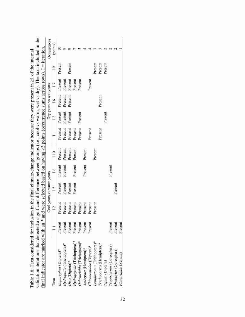
Tabl

e 1.

6. T

axa

cons

ider

ed fo

r inc

lusi

on in

the

final

clim

ate-

chan

ge in

dica

tor b

ecau

se th

ey w

ere

pres

ent i

n 1

of th

e in

tern

al

valid

atio

n ite

ratio

ns th

at d

etec

ted

a si

gnifi

cant

diff

eren

ce b

etw

een

grou

ps (i

.e.,

cool

vs w

arm

, wet

vs d

ry).

The

taxa

incl

uded

in th

e fin

al in

dica

tor a

re m

arke

d w

ith a

n *

and

wer

e se

lect

ed b

ased

on

havi

ng

3 po

ints

(occ

urre

nce

sum

s acr

oss r

ows)

. I =

iter

atio

n.

Coo

l yea

rs v

s war

m y

ears

D

ry y

ears

vs w

et y

ears

Ta

xaI 1

I 2

I 5

I 6

I 1

0 I 1

I 3

I 6

I 7

I 9

O

ccur

renc

es(p

oint

s)

Eupa

ryph

us (D

ipte

ra)*

Pr

esen

t Pr

esen

t Pr

esen

t Pr

esen

t Pr

esen

t Pr

esen

t Pr

esen

t Pr

esen

t Pr

esen

t Pr

esen

t 10

H

ydro

ptili

a (T

richo

pter

a)*

Pres

ent

Pres

ent

Pres

ent

Pres

ent

Pres

ent

Pres

ent

Pres

ent

Pres

ent

Pres

ent

9

Dix

a (D

ipte

ra)*

Pr

esen

t Pr

esen

t Pr

esen

t

Pres

ent

Pres

ent

Pres

ent

Pres

ent

Pres

ent

Pres

ent

9 H

ydro

psyc

he (T

richo

pter

a)*

Pres

ent

Pres

ent

Pres

ent

Pres

ent

Pres

ent

Pres

ent

Pres

ent

7

Och

rotr

ichi

a (T

richo

pter

a)*

Pres

ent

Pres

ent

Pr

esen

t Pr

esen

t

Pres

ent

5

Ambr

ysus

(Hem

ipte

ra)*

Pr

esen

t Pr

esen

t

Pres

ent

Pres

ent

4

Chi

rono

mid

ae (D

ipte

ra)*

Pr

esen

t Pr

esen

t

Pres

ent

Pres

ent

4

Lepi

dosto

ma

(Tric

hopt

era)

*

Pres

ent

Pres

ent

Pres

ent

3 Tr

icho

cori

xa (H

emip

tera

)*

Pr

esen

t

Pres

ent

Pr

esen

t 3

Tipu

la (D

ipte

ra)

Pres

ent

Pres

ent

2 Tr

opis

tern

us (C

oleo

pter

a)

Pres

ent

Pres

ent

2 O

reod

ytes

(Col

eopt

era)

Pr

esen

t

Pres

ent

2

Plan

ariid

ae (S

eria

ta)

Pres

ent

1

32

Tabl

e 1.

7. N

umbe

r of t

imes

(in

28 sa

mpl

ing

even

ts) t

hat t

he c

ompo

nent

taxo

n w

as p

rese

nt in

coo

l/wet

yea

rs (s

even

yea

rs to

tal)

and

war

m/d

ry y

ears

(sev

en y

ears

tota

l) an

d th

e ab

solu

te d

iffer

ence

bet

wee

n th

e ye

ar g

roup

s for

the

final

clim

ate-

chan

ge in

dica

tor.

Gen

us (O

rder

) C

ool/w

et y

ears

W

arm

/dry

yea

rs

Diff

eren

ce

(|coo

l/wet

– w

arm

/dry

|)

Ambr

ysus

(Hem

ipte

ra)

4 10

6

Chi

rono

mid

ae (D

ipte

ra)

14

21

7D

ixa

(Dip

tera

) 6

20

14Eu

pary

phus

(Dip

tera

) 12

20

8

Hyd

rops

yche

(Tric

hopt

era)

13

18

5

Hyd

ropt

ilia

(Tric

hopt

era)

8

16

8Le

pido

stom

a (T

richo

pter

a)

5 13

8

Och

rotr

ichi

a (T

richo

pter

a)

17

25

8Tr

icho

cori

xa (H

emip

tera

) 9

16

7

33

Tabl

e 1.

8. M

ean

(SE)

val

ue o

f the

loca

l clim

ate-

chan

ge in

dica

tor i

n th

e di

ffer

ent y

ear g

roup

s. *

indi

cate

s sig

nific

ant c

ompa

rison

s (p

< 0.

05).

Tem

pera

ture

Pr

ecip

itatio

n Te

mpe

ratu

re/p

reci

pita

tion

Site

Coo

l yea

rs

War

m y

ears

p

Wet

yea

rsD

ry y

ears

p

Coo

l/wet

yea

rs

War

m/d

ry y

ears

p1D

3.

8 (0

.9)

6.2

(0.9

) 0.

05*

1.

1 (0

.7)

6.5

(0.3

) 0.

004*

3.

5 (0

.9)

6.0

(0.7

) 0.

05*

2D

2.2

(0.9

) 6.

5 (0

.8)

0.00

5*

1.

9 (0

.7)

7.0

(0.5

) <0

.001

* 1.

9 (0

.8)

6.8

(0.7

) <0

.001

* 1P

4.

0 (0

.8)

6.2

(0.8

) 0.

01*

3.

8 (0

.7)

6.0

(0.4

) 0.

038*

4.

1 (0

.8)

5.4

(0.9

) 0.

3 2P

4.

9 (1

.0)

7.0

(0.9

) 0.

10

4

.0 (0

.6)

7.5

(0.6

) 0

.003

*

4.4

(0.9

) 7.

0 (0

.8)

0.05

* A

vera

ge

3.7

6.5

2.

7 6.

8

3.5

6.3

34

CHAPTER 2

Short-term impacts of stream-crossing reconstruction on forested, mountain streams in Northern California

35

Short-term impacts of stream-crossing reconstruction on forested, mountain streams in Northern California

Abstract

Stream-crossings can have multiple physical and biological impacts on small streams, ranging from increased fine-sediment delivery to increased habitat patchiness of biological communities. Culverts along small streams are often removed in accordance with Best Management Practices (BMPs) if the culverts are at risk of catastrophic failure or if they are acting as migration barriers for fish. Although BMPs attempt to minimize negative consequences of construction activities on aquatic habitats, there is limited information available on the short-term impacts of culvert removal at stream-crossings, which makes it difficult to assess the costs and benefits. The objective of this study was to quantify the short-term (0-2 years) impacts of BMPs for culvert removal on the physical and biological characteristics of six streams in the Klamath National Forest, Siskiyou County, California. I used a before-after-control-impact (BACI) study design and found no significant difference across all the sites in the total amount of fine-sediment on the streambed surface, upstream and downstream of the culverts, over the two years following culvert removal. However, in at least four sites, an order of magnitude more sediment in the <500 μm size fractions was deposited in sediment traps downstream than upstream during construction. Mild incision occurred upstream of the stream-crossings within two years, which reflected the channel's dynamic response to removal a grade-control structure. Downstream, however, there was no consistent trend of incision or aggradation. In several streams examined, Coefficients of Variation (CVs) of several commonly used benthic macroinvertebrate metrics were higher than CVs expected from natural variability based on values from long-term datasets of studies done in California. For example, the CVs of the common metrics # of Hilsenhoff Biotic Index (HBI) tolerant taxa, # of Ephemeroptera taxa, % Ephemeroptera/Plectoptera/Trichoptera (EPT), and EPT richness were higher in two of the six streams examined than the CVs expected to represent the natural range of variability present. In addition, I observed significant declines among the six sites in the proportion of EPT taxa and EPT individuals that colonized sediment traps downstream of the culverts. Although there were few statistically significant differences in stream characteristics that could be generalized across all sites, there were substantial, site-specific responses in sediment deposition, channel response, and benthic macroinvertebrate assemblages. These responses may relate to intrinsic natural differences among the streams or to differences in the implementation of Best Management Practices during construction. Despite the limited site-specific, short-term impacts on aquatic biota, stream-crossing reconstruction offers long-term benefits such as reduced flood-risk and improved fish-passage.

Key words: stream-crossing reconstruction, forest roads, culverts, sedimentation, benthic macroinvertebrates, headwater streams, Best Management Practices

36

Introduction

Forest roads and the culverts that often underlie them at stream-crossings can greatly impact stream-channel morphology, hydrology, and sediment-transport processes. For example, forest roads can intensify sediment delivery to stream channels through erosion (e.g., Reid and Dunne 1984, Switalski et al. 2004, Madej et al. 2006) and can increase the flashiness of streams following storms through decreased permeability (Wemple et al. 1996). Culverts can lead to the formation of plunge pools (Kahn and Colbo 2008), the decline of riffle-habitat in downstream areas (Merrill 2005), and the accumulation of fluvial sediment in upstream areas (Jackson 2003).

Forest roads and culverts can also impact biological characteristics of streams, including the vertebrate and invertebrate communities. For example, Wofford et al. (2005) observed that barriers to passage in headwater streams caused within-watershed genetic variation in coastal cuttthroat trout. Warren and Pardew (1998) observed fish passage to be an order of magnitude lower through pipe culverts than through open-arch culverts or natural stream reaches in small, mountain streams. Likewise, Thomson and Lee (2000) observed a negative correlation between forest-road density and fish stocks throughout the northwestern United States. Culverts have also been observed to impede the upstream movement of benthic macroinvertebrates in proportion to the amount of shear stress and the size of the elevation drop at the downstream end (Resh 2005). Nationwide, there are 700,000 km of forest roads on United States Forest Service (USFS) lands (Elseroad et al. 2003). The term "forest roads" refers to paved and unpaved roads that connect national forests to the existing state highway system (23 USC § 101). Many of these forest roads were constructed for timber extraction on USFS lands and are no longer being used nor maintained (USFS 2001). These roads are managed in accordance with Best Management Practices (BMPs) of the USFS, which can be defined as practices that are determined to be an effective way of preventing or reducing nonpoint source pollution to a level compatible with water-quality goals (USFS 1980). Removal of pipe culverts at stream crossings and replacement with open-arch culverts is a practice that is widely performed because of the perceived long-term benefits of flood prevention and fish-passage improvement (Ice et al. 2004). However, the effectiveness of the BMPs which are applied during reconstruction in preventing short-term physical and biological degradation of aquatic systems has not been examined in detail (Luce 1997). The objective of this study was to quantify the short-term (0-2 years) impacts of stream-crossing reconstruction projects, using current USFS Best Management Practices (BMPs), on a variety of physical and biological characteristics of six streams in the Klamath National Forest (KNF) of Northern California. These characteristics included stream-channel morphology, hydrology, and composition of benthic macroinvertebrate assemblages. I examined physical and biological characteristics of these streams before (Y0-pre), just after (Y0-post), one year after (Y1), and two years after (Y2) culvert removal using a Before-After-Control-Impact (BACI) study design. The null hypothesis was that there would be no difference in the physical and biological characteristics in these streams before and after the stream-crossings were reconstructed.

37

Methods

General Site Description The KNF of Northern California is a mountainous, densely forested region with little human development (Fig. 2.1). Covering an area of about 690,000 ha, it has a total relief of 2500 m. The forest is drained by the Klamath River and its main tributaries, which include the Salmon, Scott, and Shasta rivers. The Klamath Mountains are characterized by steep, rugged terrain formed of folded and faulted Mesozoic and Paleozoic Era rocks (USFS 1998). The climate is characterized by cool, wet winters and warm, dry summers. Annual precipitation ranges from an average of about 250 mm in low elevations to 2,500 mm at high elevations, increasing from east to west. Precipitation falls mainly in the form of rain below 1,250 m and snow above 1,250 m. The riparian community consists of a variety of tree species in mixed-conifer stands including (but not limited to) alder (Alnus spp.), willow (Salix spp.), Douglas fir (Pseudotsuga menziesii), and sub-alpine fir (Abies spp.). The biodiversity of this region is among the highest in the world for temperate coniferous forests (DellaSala 1999). The hydrology of the KNF is characterized by high-flows in winter and spring followed by an extended low-flow season in summer. Peak floods, which occur in winter, are rain-on-snow events, whereas average floods, which occur in spring, are snowmelt dominated. Rain-on-snow events are one of the most significant weather-related hazards that affect the forest-road system (USFS 1998). Within the past 35 years, there have been about 10 summer debris flows on the KNF generated by intense convective storms in the summer (North and South Fork Salmon River, Seiad Creek, and Beaver Creek). These events are different than the winter debris flows in that large amounts of sediment are delivered to streams and rivers during slow flow conditions (J. Fuente, personal communication). Such events can cause high flows and large amounts of sediment and debris transport, which can fill or overload culverts. In the past, stream crossings on forest roads were typically designed to convey a 25-year flood, and the designs did not typically plan for debris from upstream (USFS 1998). New construction at stream crossings is designed to convey a 100-year flood and to accommodate debris from upstream (USFS 1998). Landslides are another weather-related hazard for forest roads, and although they occur naturally, management activities have more than doubled the sediment production as a result of landslides in the KNF (USFS 1998). Six streams that were scheduled for stream-crossing reconstruction in the KNF were selected for monitoring. These streams were prioritized for reconstruction by USFS because of their potential as migration barriers to fish and their risk of catastrophic failure. Culverts at these streams were originally scheduled to be replaced during the same year, but as a result of construction delays four culverts were replaced in 2004 and the other two were replaced in 2005. Because each stream was monitored prior to reconstruction and two years following reconstruction, this study was conducted over four years. The stream-crossings at the sites all contained pipe culverts of similar dimensions, ranging from 2.1 m to 3.6 m in diameter and 13 m to 31 m in length, and were all replaced with open-arched culverts of similar design (Fig. 2.2). Prior to stream-

38

crossing reconstruction, migration barriers at the downstream ends of the culverts, which were in the form of scour pools, ranged in height from 1.0 m to 2.8 m (Table 2.1). Several high flows occurred during the study period that may have resulted in bed mobilization and sediment transport. The USGS operates three stream gages in the region that provide relevant information (Fig. 2.3). The Indian Creek gage is likely the most representative of the hydrology at the sites because it is located on the smallest stream, although it is still fairly large relative to the study sites. The other gages are located on large rivers. In steep, boulder, step-pool streams, similar to those in the study, there are two phases of bed mobility: finer grained sediment stored in pools gets mobilized near bankfull, while the larger, cobble and boulder classes that makeup the steps get mobilized much less frequently, i.e., >10 years (Lisle 1995, Montgomery and Buffington 1997). The typical recurrence interval of these bankfull discharges is approximately 1.5 years (Dunne and Leopold 1978). At the Indian Creek gaging station, bankfull discharge would occur at flows >130 m3/s, based on 55 years of USGS flow records. At lower discharges, partial scour of the bed and consequent disturbance of benthic macroinvertebrates could occur (Power et al. 2008). During the study period, bankfull discharges at the Indian Creek gage occurred in water years 2005, 2006, and 2007. The 2006 flood was the largest that occurred during the study. It had a peak discharge of 560 m3/s at Indian Creek and an 11-year return period. The mean annual flood at Indian Creek was 225 m3/s. The 2006 flood had a return period of 11 years at the Scott River near Fort Jones, CA, based on 67 years of gage records, and 14 years at the Klamath River near Seiad Valley, CA, based on 70 years of gage records. A study by Keppeleer, Cafferata, and Baxter (2007) showed a peak in sediment load following the 2006 winter flood along a forest road in Jackson State Forest, another mountainous forested region in Northern California. The results of their study suggest that such flood events can be very detrimental in terms of altering channel configuration and increasing sediment load to the best management attempts for reconstructing stream crossings.

Channel Morphology Stream crossings were surveyed before culvert removal to quantify the dimensions (length and diameter) of the culverts, the slope of the culverts, and the amount of fill material surrounding the culverts. These surveys of the stream-crossings were also used to assess the long-term benefits of the projects, such as improved fish passage and reduced risk of catastrophic failure that could occur during storm events. Channel cross-sections were surveyed with an auto level prior to stream-crossing reconstruction (Y0-pre), one year after reconstruction (Y1), and two years after reconstruction (Y2). Seven cross-sections were surveyed upstream of each stream-crossing (XU1-XU7) and five were surveyed downstream (XD1-XD5). The first cross-sections upstream (XU1) and downstream (XD1) were installed 2 m from the upstream and downstream ends of the culvert, respectively. The edges of all the cross-sections except for XU1 and XD1 were monumented throughout the study. Removal of fill material during construction disturbed the original monuments at XU1 and XD1. The first monumented upstream cross section (XU2) was surveyed just after stream-crossing reconstruction (Y0-post) only at sites where extraction of fill material during construction notably altered the cross-section. Spacing between cross-sections was determined using the average bankfull width, with the upstream and downstream reaches treated separately.

39

If bankfull width was < 3m, the cross-sections were spaced 3 bankfull widths apart, and if bankfull width was > 3m, the cross-sections were spaced 4 bankfull widths apart. Longitudinal profiles were surveyed with an automated level prior to stream-crossing reconstruction (Y0-pre), just after reconstruction (Y0-post), one year after reconstruction (Y1), and two years after reconstruction (Y2). The longitudinal profiles followed the thalweg of the channel, starting 20 m above the most upstream cross-section and extending 20 m below the most downstream cross-section. Thalweg migration resulted in annual variation in distances measured along the longitudinal profile, which caused the cross-sections to differ in their locations along the longitudinal profile from year to year. To facilitate comparisons between years, I scaled the distances along each profile to maintain constant distances between the cross-sections over time. In addition, I set the thalweg elevation changes along the longitudinal profile to match those measured at each of the cross-sections because the longitudinal profiles, unlike the cross-sections, were not surveyed relative to a monumented benchmark.

Sediment To determine changes in sedimentation, I used measurements of riffle-surface fine-sediment (<4 mm) (Cover et al., 2008), grain size distributions (Wolman 1954), and measurements of fine-sediment deposited in sediment traps upstream and downstream of the stream-crossing. Measurements of riffle-surface fine-sediment and grain size were performed annually to monitor changes occurring in the two years after stream-crossing reconstruction. Sediment trap measurements were performed once and were used to monitor short-term (2-4 months) sedimentation that occurred during reconstruction. Riffle-surface fine-sediment measurements were collected prior to stream-crossing reconstruction (Y0-pre), the year after reconstruction (Y1), and the second year after reconstruction (Y2). Presence or absence of riffle-surface fine-sediment was recorded at each of 210 point measurements at grid intersections on a 9' x 4' net with a 5" grid. Two grid-transects were measured at each cross-section, one starting at the cross-section with the net facing upstream and the other one starting at the cross-section with the net facing downstream.

Grain-size distributions were measured on the stream bed-surface using pebble counts at four cross-sections upstream (XU4-XU7) and four cross-sections downstream (XD2-XD5) of the road crossing. A minimum of 100 grains were measured per cross-section, for a total of 400 grains per upstream and downstream reach. I combined the pebble count data into upstream and downstream groups and determined the D50 (the median grain-size), the D16 (the grain-size class for which 16% of the particles are smaller), and the D84 (the grain-size class for which 84% of the particles are smaller). I chose these metrics because the D50 is useful for bedload transport calculations and the D16 and D84 are useful in biological habitat evaluations (e.g., Kondolf 2000). To assess the impacts of fine sediment on subsurface habitat, particularly incubation habitat for gravel-spawning fish and burrowing habitat for invertebrates, I measured streambed permeability (methods modified from Barnard and McBain 1994). Reach-average subsurface gravel permeability was calculated from each of 10 in-situsample sites located upstream and downstream of each road crossing. Sample sites were located in patches of gravel that ranged from 40 to 80mm in medial particle size. At each site, a 3 cm diameter perforated standpipe was driven into the streambed to a depth of

40

36cm, with a sampling depth of 14 to 22cm below the bed elevation. This grain size and depth were chosen because it reflects the average egg-pocket depth and substrate size used for spawning by several species of salmonids (Kondolf and Wolman 1993). Water was pumped out of the upper 2.5 cm of the water column in the standpipe with a battery-powered vacuum pump into a measurement chamber. The rate at which interstitial water refilled the void was measured, and five replicate samples were drawn for each standpipe location. Permeability (cm/hr) was calculated from the inflow rate (ml/s) using calibration curves (Barnard and McBain 1994). Sediment traps consisted of a 17 cm diameter bowl filled with sieved and clean bed material 20 - 30 mm in diameter (Fig. 2.4). Sediment traps were installed during the dry period of the year, under base-flow conditions (Table 2.1) in locations that were visually assessed to be depositional habitats (i.e., pools margins, etc). However, it was not possible to control for the quality of depositional environments, i.e., some streams may have had conditions that favored greater deposition than others. These traps were buried in the streambed in low-velocity, depositional habitats (pools, margins, etc.) within the wetted channel prior to stream-crossing reconstruction (Y0-pre) so that the edges of the bowl were flush with the bed surface. Five traps were installed upstream and five were installed downstream of the stream crossings. The sediment traps were installed from XU4 through the top of the reach (20 meters above XU7) and from XD3 through the bottom of the reach (20 meters below XD5), and were removed from the bed two to four months after stream-crossing reconstruction was complete (Table 2.1). During trap removal, the original (20 - 30 mm) gravel pieces that were placed in the traps were separated from the accumulated debris by washing the gravel particles with a pressurized spray of water. Accumulated debris was passed through a sieve to initially divide the material into two size fractions, <0.5 mm and >0.5 mm. The >0.5 mm material was stored in 95% ethanol to preserve the benthic macroinvertebrates that had colonized the sediment trap. The <0.5 mm material was stored in water. In the laboratory, the >0.5 mm fraction was examined under a stereo microscope at 10x magnification and all invertebrates were removed. Large pieces of organic matter (leaves, twigs, etc.) were also separated out from the sediment sample, and were dried and weighed. The >0.5 mm sample was then processed identically to the <0.5 mm sample. Both samples were treated with a series of hydrogen peroxide baths to dissolve the particulate organic matter. Baths were continued until further additions of hydrogen peroxide failed to produce a reaction. The remaining inorganic sediment was wet sieved into eight grain-size classes ranging from 0.063 to 4mm, dried, and weighed. Unfortunately, information from two of the sites, LBC and STC, was lost during processing.

Benthic Macroinvertebrates To determine changes in macroinvertebrate communities, I used two sampling approaches: (1) targeted-riffle samples and (2) colonization samples from the sediment traps. Targeted-riffle samples measured changes in resident macroinvertebrate communities over the first two years before and after stream-crossing reconstruction. Colonization samples measured short-term changes in colonizing macroinvertebrate communities occurring over the first two to four months during and after reconstruction. The targeted-riffle samples consisted of a composite of eight 0.09 m2, fixed-area samples taken from four different fast water habitats including riffles, rapids, cascades,

41

and steps (Rehn et al. 2007). Two separate 0.09 m², fixed-area samples were taken from each habitat unit with rapidly flowing water for a total of eight samples per upstream and downstream reach. Samples were collected before stream-crossing reconstruction, one year after reconstruction, and two years after reconstruction. This sampling approach conformed to the standard USFS bioassessment protocol and was chosen to also allow samples to be analyzed using River Invertebrate Prediction and Classification System (RIVPACS) type models (Hawkins et al. 2000). Laboratory sorting and identifications of the targeted-riffle samples were done at the National Aquatic Monitoring Center (Utah State University, Logan, Utah), following their established laboratory methods, which are described in Vinson and Hawkins (1996). Organisms were identified to the lowest practical taxonomic level, usually genus or species, except for Chironomidae (subfamily), Collembola (order), Trombidiformes (order), Oligochaeta (class), Ostracoda (class), Turbellaria (class), and Nematoda (Phylum). The macroinvertebrates from the colonization samples were sorted at 10x magnification under a stereomicroscope, and the insects in these samples were identified to genus, and other macroinvertebrates to family (gastropods, crayfish, amphipods), order (ostracods, water mites), or class (segmented worms), using identification keys in Merritt et al. (2007) and Thorp and Covich (2001). I selected biological metrics a priori based on the likelihood that they would be able to detect a change in the colonizing macroinvertebrate community associated with a sedimentation impact (Waters 1995, Angradi 1999). These metrics included three metrics of diversity (taxa richness, Shannon Diversity Index, and % dominant taxon), three metrics of pollution-tolerance (% EPT taxa [the insect orders Ephemeroptera, Plecoptera, and Trichoptera], % EPT individuals, and HBI [Hilsenhoff Biotic Index], (Hilsenhoff 1982, 1987), and the proportion of functional feeding groups in each sample (% collector filterers, % collector gatherers, % predators, % scrapers, and % shredders). In addition, I chose ten insect genera that had previously been determined to be sensitive to riffle-surface fine-sediment in the Klamath National Forest (Cover et al., 2008), and used these taxa separately as individual metrics. For most of these metrics, I expected a decrease in the metric value in response to fine-sediment. However, for percent dominant taxon and HBI I expected an increase. For the functional feeding groups, I expected a noticeable shift in the proportions contained within each group.

Data Analysis I used statistical hypothesis testing to analyze all the data except for the channel-morphology information. I avoided pseudoreplication in each experiment by combining all the upstream and downstream data into groups and treating the sites as replicates rather than treating each individual measurement at each site as a replicate. Pseudoreplication was not an issue in the analysis of the channel morphology because I did not use inferential statistics. Prior to running the statistical tests I tested the distributions for normality using the Shapiro-Wilk (1965) test, which informed my choice between a parametric test (assumption of normality) and a non-parametric test. Because deposition of fine-sediment associated with stream-crossing reconstruction was likely to affect only the downstream reach, I treated upstream of the stream-crossing as the control and downstream as the test condition. These statistical tests conformed to the Before-After-Control-Impact (BACI) study design (Smith et al. 1993).

42

Channel Morphology To quantify the potential long-term benefits of the stream-crossing reconstructions, I determined the height of the migration barrier below the downstream end of the culvert prior to removal (Y0-pre), and compared this to the maximum jumping heights for rainbow trout (Whyte et al. 1997), which are found in this region. I also calculated the volume and percent of fill that was removed during the construction process as a measure of the potential sediment delivery to the stream if the stream crossing had failed. This is a worst case scenario, since a proportion of the fill usually remains on-site during such events. To determine changes in channel morphology, I separately examined the upstream portion of the longitudinal profiles, the downstream portion of the profiles, and the entire length of the longitudinal profiles over three time periods: (1) prior to stream-crossing reconstruction (Y0-pre) to just following reconstruction (Y0-post), (2) prior to reconstruction (Y0-pre) to one year after reconstruction (Y1) , and (3) prior to reconstruction (Y0-pre) to two years after reconstruction (Y2). In each case, I plotted the longitudinal profile, fit a trend-line through it using linear regression, determined the slope of the profile from this trend-line, and compared the changes in slope over the three time periods. In addition, I used the y-intercept of the trend line to determine if incision or aggradation had occurred in each study reach following culvert removal. A decrease in the y-intercept indicates incision, whereas an increase indicates aggradation. Any elevation change <0.5 m over the length of the longitudinal profile was decided a priori to be insignificant because it is within the range of measurement error for repeated surveys. To determine if incision or aggradation was occurring as a result of the stream-crossing reconstruction, I examined the monumented upstream and downstream cross-sections (XU2-XU7 and XD2-XD5) and calculated the areas of these cross-sections using trapezoidal integration. I focused on the first monumented upstream (XU2) and downstream (XD2) cross-sections because I hypothesized that these would be most impacted by grade changes resulting from stream-crossing reconstruction because of their proximity to the stream crossing. I also examined the distribution of pools upstream and downstream of the stream-crossings prior to reconstruction (Y0-pre), just after reconstruction (Y0-post), one year after reconstruction (Y1), and two years after reconstruction (Y2). Pools were defined using a minimum depth criterion of 0.5 m (Montgomery and Buffington 1997). I calculated the total number of pools and the average depth of pools in each upstream and downstream reach at all of the sites. The upstream and downstream reach lengths investigated ranged from 77 m to 153 m. In addition, I determined the maximum depth of the first pool downstream of the stream crossing, which would have been the plunge pool prior to removal of the culvert (Y0-pre).

Sediment To determine changes in short-term fine-sediment deposition (i.e., just before and after stream-crossing reconstruction) I compared the average volume of fine-sediment deposited in the five sediment traps upstream and downstream of each stream crossing. The sediment traps were installed during the dry-period of the year, under base-flow conditions (Table 2.1). Although some streams may have had more or better depositional

43

environments than others, the sediment traps were installed in locations that were visually estimated to be primarily depositional environments. To determine the changes in riffle-surface fine-sediment over the two years following stream-crossing reconstruction (Y1 and Y2), I used a Before-After-Control-Impact (BACI) study design (Smith et al. 2003). First, I computed the percent riffle-surface fine-sediment along reaches upstream and downstream of the stream-crossings and found the difference (di) between these percentages. Then, I performed an ANOVA on di to test for differences between upstream and downstream between any years of the study. I used the same BACI design to determine changes in grain-size distributions on the bed-surface upstream and downstream of the culverts over the two years following stream-crossing reconstruction between combinations of any of the years of the study (e.g., Y0-pre and Y1, Y0-pre and Y2, and Y1 and Y2). Because this data did not meet the normality assumptions, I performed a non-parametric Wilcoxon Signed Rank test on the difference between the D50 upstream and downstream at each site.

Benthic Macroinvertebrates I analyzed the macroinvertebrate data from the targeted-riffle samples using an approach based on Coefficients of Variation (CV = SD/mean x 100, expressed as a percent). This approach was selected over the standard approach of directly comparing metric values because it allowed me to cumulatively analyze the within-site variability of multiple metrics over time. The CV-based analytical approach involved selection and calculation of 14 metrics, comparison of metric values over the time periods of the study, examination of site-specific effects, and comparison of effects with responses of individual taxa (Fig. 2.5). First, I calculated Coefficients of Variation for each metric based on the six sites. Then, I compared each of these CVs with a composite value of a CV obtained for these metrics from relatively undisturbed sites reported in a variety of long-term studies conducted in California outside of the Klamath region (Resh 1979, Rosenberg and Resh 1982, Lamberti and Resh 1985, Resh and Jackson 1993, Resh et al. 1995, Resh et al. 2000, Mazor 2006, Mazor et al. 2009, and Resh, unpublished data). I selected the approximate median estimate of annual variability for each metric reported in previous studies: richness (30%), abundance (50%), Simpson's diversity index (30%), # of HBI intolerant taxa (30%), # of HBI tolerant taxa (30%), # of Ephemeroptera taxa (50%), Ephemeroptera abundance (50%), # of Trichoptera taxa (50%), Trichoptera abundance (50%), # of Plecoptera taxa (50%), Plecoptera abundance (50%), EPT abundance (50%), EPT richness (30%), and % EPT (50%). In addition to comparing the CVs from this study to the CVs representing reported values of natural variability, I also compared the CVs found in this study to CVs that would represent 50% of the natural variability reported, which is a more conservative approach to detect variability. The individual taxa were composed of ten genera that were selected a prioribecause they have previously been determined to be sensitive to fine-sediment in the KMF (Cover et al. 2008). These genera were analyzed in terms of absolute differences in abundance over the time periods of the study. I sought to determine which of these taxa were most responsive and which sites tended to show the largest effects on taxa. I analyzed the macroinvertebrate data from the colonization traps using composited samples from upstream and downstream to avoid pseudoreplication. A

44

paired t-test (paired by stream) was used to test for significant differences ( = 0.05) in metric values from samples upstream and downstream of each culvert for all six sites. For all metrics except EPT Individuals, the statistical power ( ) of each of these tests determined post-hoc was below = 0.80. Thus, any lack of significant differences should be interpreted with caution.

Results

Channel Morphology The potential migration barriers that were removed, i.e., the elevation drop at the downstream end of the culverts prior to reconstruction, and the volumes of fill material removed varied among the sites (Table 2.1). For example, the largest migration barrier of 2.8 m in LBC was 1.8 m higher than the smallest barrier in STC. The values ranged from 1.0 m to 2.8 m. UEC had the largest percentage of its fill removed (99%) of all the sites.The values ranged from 4% to 99%. Channel slope upstream of stream-crossings, and at some of the sites downstream of the crossings, became steeper following culvert removal (Table 2.2). In BIC, for example, the slope of the upstream reach was originally less steep than downstream, but the slopes equilibrated by the second year after culvert removal (Y2). The largest difference in slope between upstream and downstream prior to construction (Y0-pre) was in LBC. However, by the second year after culvert removal (Y2) this difference was reduced by nearly 50% due to steepening in the upstream reach. Over the entire length of the longitudinal profile (Fig. 2.6), the change in the slope of was small ( 1.5%) at all sites, and no incision or aggradation was evident (all changes in the y-intercept of the trend lines were 0.5 m). Culvert repositioning to a lower slope could account for the change.

Cross-sections showed notable changes extending 20-40 m upstream of some of the culverts, and minimal changes extending downstream (Fig. 2.7). The changes were a result of a combination of the extraction of fill material during construction and the 2006 floods. Over the two years following stream-crossing reconstruction (Y0-pre to Y2), BIC, CEC, UEC, and LBC incised upstream about one meter on average and STC aggraded about half a meter (Fig. 2.8). The largest magnitude change was in LBC, which incised over two meters in a portion of the channel. Incision was accompanied by an increase in cross section area. The cross-section area of XU2, for instance, increased as a result of fill extraction during culvert removal in LBC (increase of 14 m2), BIC (increase of 12 m2), and UEC (increase of 13 m2) (Table 2.3). The 2006 floods caused further incision in BIC (increase of 3m2), CEC (increase of 2 m2), and UEC (increase of 1 m2)(Fig. 2.8, Table 2.3). UBC was the most stable of all the sites. Downstream of the stream-crossings, the changes in cross-sections were smaller (Fig 2.9). CEC incised about 0.25 m on the right bank, which was compensated for by about 0.5 m of aggradation on the left bank. UEC incised about 0.25 m, UBC and LBC aggraded about 0.5 m on average, and BIC changed by less than 0.1 m. The areas of the first monumented downstream cross-section (XU2) increased by small amounts (1-2 m2)compared to upstream. For example, the cross section area of STC increased by 2 m2

between the year prior to construction (Y0-pre) and the year after construction (Y1). The XU2 cross-section in BIC, CEC, UBC, and LBC increased in area by 1 m2 during this

45

study period. Many of these changes in cross-section area downstream returned closer to pre-construction (Y0-pre) levels between the first (Y1) and second (Y2) year after stream-crossing reconstruction The distribution of pools changed notably following stream-crossing reconstruction. The depth of the first pool downstream of the road-crossing, for example, decreased in all six sites following reconstruction (Table 2.4). The first downstream pool in LBC, which was the largest of the six sites, was reduced in depth by about 1 m as a result of the addition of boulders to the channel during construction. The total number of pools along the entire longitudinal profiles, including upstream and downstream of all sites, decreased from 37 before reconstruction (Y0-pre), to 28 just after reconstruction (Y0-post), before settling at 22 the first year after reconstruction (Y1) and 23 the second year after reconstruction (Y2).

Sediment There was no significant difference overall in fine-sediment on the surface of riffles between upstream (X = 13%) and downstream (X = 14%) reaches among years (Prob>F = 0.30). However, there was evidence for increased levels of riffle-surface fine-sediment in downstream reaches following construction in three out of six sites (Fig. 2.10). For example, riffle-surface fine-sediment in the downstream reach of Upper Elk Creek increased from 8% to 24% between the year prior to stream-crossing reconstruction (Y0-pre) and the first year (Y1) after reconstruction (Fig. 2.10). In STC, the amount of riffle-surface fine-sediment was eight percentage points higher downstream than upstream in Y1 and 15 percentage points higher downstream than upstream in Y2. The difference was negligible in Y0-pre at this site (26% upstream vs. 27% downstream). In BIC, it was 11 percentage points higher downstream than upstream in Y1 and three percentage points higher in Y2. The difference was again negligible in Y0-pre (11% vs. 13%). There was no evidence for increased deposition of fine-sediment following construction at the remaining three sites. Trends in riffle-surface fine-sediment following stream-crossing reconstruction were influenced more strongly by the flood year of 2006 than by the amount of time that passed since the stream-crossing was reconstructed (i.e., the difference between Y0-pre and Y1 or Y1 and Y2). The 2006 flood reduced the riffle-surface fine-sediment in the channel downstream in four out of six streams. The large increase in fine-sediment in UEC downstream of the stream-crossing the year following reconstruction, for example, was reduced to nearly Y0-pre levels following the 2006 flood season (Fig. 2.10). Fine-sediment was 18% downstream in STC just following the flood season in 2006, and 27% the year before. In BIC, it was 13% following the 2006 flood year, and 19% the year before. In CEC and UBC, the 2006 floods did not have a notable effect. I did not detect a significant change overall in the D50 between upstream and downstream following the stream-crossing reconstructions (p = 0.653). In the year prior to reconstruction, the difference in the D50 between upstream and downstream ranged from 9 mm to 129 mm (Table 2.5). Only one site, CEC, had a large difference between upstream and downstream. Neither the D16 (p = 0.237) nor the D84 (p = 0.567) were significantly different between upstream and downstream. The average D16 over all sites and years was the same upstream (X = 5 mm) and downstream (X = 5 mm) of the stream-crossing, and the average D84 was nearly the same (X = 443 mm vs. X = 447 mm). This

46

narrow range indicates that the D16 and D84 were more uniform among the sites than the D50. The 2006 flood did not distinctly impact any of the grain size distributions. Likewise, distinct trends in the D50 were not evident following stream-crossing reconstruction (Table 2.5). For example, from Y0-pre to Y1, half of the sites showed an increase in the D50 upstream of the stream-crossing and half showed a decrease. During this same period, four of the sites showed a decrease in the D50 downstream of the stream-crossing and two showed an increase. Between Y0-pre and Y2, four of the sites upstream of the culvert showed an increase in the D50 and two of the sites showed a decrease. During this same period, five of the sites showed an increase in the D50downstream of the stream-crossing and one showed an increase. Following the flood year of 2006, five out of six sites showed an increase in the D50 upstream of the stream-crossing, whereas only half the sites showed an increase downstream. Subsurface permeability values were highly variable within and among years and no consistent patterns were observed between upstream and downstream sampling locations (Fig. 2.11). The average CV within a sample site was low (7 %), indicating a high degree of precision within an individual site. However, these in-situ measurements represent subsurface flow rates in small patches of the streambed, and can be biased toward artificially high values in coarse bedded streams (Kondolf et al. 2008). My results indicate that these coarse bedded, predominantly step-pool morphology streams, have highly variable subsurface flow conditions. Subsurface flow rates are greatly affected by the abundance of fine sediment stored in interstitial spaces, and high values result in greater egg survival of salmonids and can affect burrowing habitat for invertebrates (Chapman 1988). The total amount of fine-sediment deposited in the sediment traps in the four sites with information available (BIC, CEC, UEC, and UBC) was significantly higher downstream (X=1163 g, SD = 267) than upstream (X = 148 g, SD = 44) of the stream-crossings (P<0.001), which was a 685% change. The amount of sediment deposited varied by site. UBC had the highest amount of total deposited sediment (X = 848 g, SD = 263) and CEC (X = 39 g, SD = 12) had the lowest. The amount of fine-sediment in the <500 μm size fractions deposited in the sediment traps was higher downstream than upstream in all four sites (Fig. 2.12). In UBC, for example, the amount of fine-sediment deposited downstream was 848 g (SD = 263), while only 94 g (SD = 42) was deposited upstream. In UEC, the amount of fine-sediment deposited downstream was 180 g (SD = 47), while upstream only 36 g (SD = 9) was deposited. This difference was not significant overall (p = 0.20), however, due to the low sample size and high variability among sites.

Benthic Macroinvertebrates In the targeted riffle-samples, only four out of the fourteen selected metrics responded as predicted with a distinct pattern (Table 2.7), however, the cumulative number of comparisons among all the metrics that showed changes outside the range of expected natural variability in the direction most likely to reflect an impact associated with elevated levels of fine-sediment was significantly higher downstream than upstream (Table 2.8). The four metrics that showed a distinct pattern were # of HBI tolerant taxa, Ephemeroptera taxa richness, % EPT, and EPT richness (Table 2.7). The number of comparisons of these four metrics that exceeded the expected natural variability was

47

higher downstream of the stream-crossing than upstream, and the number that exceeded one-half the expected natural variability was also higher downstream of the stream-crossing than upstream (Table 2.9). The number of comparisons that exceeded the expected natural variability was highest at LBC (4 metrics) and UEC (3 metrics) (Table 2.9). In the other creeks (e.g., BIC, CEC, UBC, and STC), it was evident in only one or two of these four metrics (Table 2.9). In addition, some metrics exceeded natural CVs more often than others, some sites showed more variability than others, and some taxa were more sensitive than others. The two EPT metrics showed the most downstream impacts (e.g., in four of the six streams), whereas the # of HBI tolerant taxa and # of ephemeroptera taxa metrics showed an impact in only two of the six streams (Table 2.9). The total number of comparisons that exceeded CVs representing natural (and one-half) variability going in the predicted direction was highest in LBC (Table 2.8). Among the sediment-sensitive taxa, Chironominae showed the clearest pattern reflective of an impact; Chironominae abundance was lower downstream than upstream in seven out of 12 comparisons after stream-crossing reconstruction, and zero out of six comparisons prior to reconstruction (Table 2.10). In the 59 colonization samples, a total of 17,851 organisms were found, comprising 54 distinct taxa. The most common taxa were the chironomid midges (10,078 individuals), lepidostomatid caddisflies (Trichoptera: Lepidostomatidae; 1,477 individuals), and chloroperlid stoneflies (Plecoptera: Chloroperlidae; 1,013 individuals). Other common organisms included the ostracods (871 individuals), biting midges (Diptera: Ceratopogonidae; 691 individuals), and Paraleptophlebia mayflies (Ephemeroptera: Leptophlebiidae; 571 individuals). The abundances of individual EPT taxa were generally lower downstream than upstream (Table 2.11). In addition, the total abundance of EPT organisms was lower downstream (984) than upstream (3,574).

Only two metrics calculated for the colonization samples were significantly different between upstream and downstream reaches. These were the proportion of EPT taxa (48.6% vs. 42.1%, P = 0.02) and EPT individuals (27.3% vs. 19.5%, P = 0.005), which were significantly lower downstream than upstream.

Discussion

Forest roads can impact the physical and biological characteristics of streams (USFS 2001). For example, stream crossings can act as migration barriers to fish and benthic macroinvertebrates (Thomson and Lee 2000), can disrupt food-web linkages between aquatic and terrestrial ecosystems (Switalski et al. 2004), and can fail completely, resulting in large pulses of sediment, and initiating or adding to debris flows (Wemple et al. 2001). Debris flows can reduce macroinvertebrate diversity (Cover et al. 2008) and cause localized extirpations of salmonids (Lamberti et al. 1991, Roghair et al. 2002) in the short-term, and can cause dramatic changes in channel morphology (May and Gresswell 2003, May and Lee 2004) in the long-term. Stream-crossing reconstruction is a practice that aims to reduce migration barriers to aquatic species and the harm and risk associated with culverts at stream crossings. In this study, we observed significant short-term effects of stream-crossing reconstruction on aquatic habitats and biota.

48

Streams in this study exhibited dynamic responses to stream-crossing reconstruction because culverts were acting as grade-control structures. Although the overall changes in channel slope and cross-section dimensions were small over the 2-year period examined in this study, site-specific effects were more notable. Geomorphic responses were particularly evident during the 2006 flood, a large magnitude (10-20 year return interval) event. Several sites experienced incision extending 20-40 m upstream of the stream crossings, caused by a combination of sediment removal by construction activities and a geomorphic response to the removal the grade-control structure. This incision was likely a result of the loss of sediment that had accumulated after the culvert was originally inserted, because sediment has been widely observed to accumulate upstream after culvert installation (Wellman et al. 2000, Jackson 2003). I did not observe a systematic increase in riffle-surface fine-sediment upstream or downstream of the stream crossings after reconstruction because, relative to streams in other mountainous landscapes, streams in the Klamath Mountains are steep in relation to their respective drainage areas and have a naturally high sediment-transport capacity (May 2007). Thus, any increase in fine-sediment supply would most likely have been transported out of riffles. The observed decrease in the amount of fine sediment on the bed surface in riffles downstream of the culverts in many of the sites following the largest flood year during the study demonstrates the channel's capacity to flush itself of fine sediments. This agrees with other studies that have shown that steep alluvial channels (cascade and step pool) have high ratios of transport capacity to sediment supply and areresilient to changes in discharge and sediment supply (Montgomery and Buffington 1997). Although changes in riffle-surface fine-sediment were only evident at some sites, large changes in fine-sediment deposition in traps were evident in all the sites examined, which suggests that fine sediment that was potentially introduced during the reconstruction was flushed through riffles and deposited in depositional areas. The increased variability indicated by the CVs of metrics describing the benthic-macroinvertebrate communities downstream of the stream-crossings may reflect the response of these communities to increased habitat heterogeneity or patchiness. Increases in sediment patchiness can certainly have effects on spatial patterns and inter-sample variability of benthic-macroinvertebrate communities (Resh 1979, Palmer et al. 1996). The higher than expected variability in the biological metrics downstream of the stream crossings may reflect the increase in the fine sediment deposited in the traps, which could have been redistributed from the bottom substrate of the plunge pools or washed out directly from the stream-crossing fill-material or the associated construction zone. The pebble-count information supports the observed increase in habitat heterogeneity. For example, the average inter-annual variability in the D50 was 47% higher downstream (SD = 38 mm) than upstream (SD = 26 mm), even though the average difference between upstream and downstream from year to year was not significantly different.

Specific metrics were more useful in indicating change in the benthic-macroinvertebrate communities than others. The four most responsive metrics (# of HBI tolerant taxa, ephemeroptera taxa richness, % EPT, and EPT richness) that indicated change in the resident benthic-macroinvertebrate communities (i.e., those from the targeted-riffle samples) in the predicted direction of impact are widely known to be reliable indicators of disturbance (Klemm et al. 2002). In the sediment trap samples, the lower EPT metric values downstream of the stream crossings indicates that the stream-

49

crossing reconstructions may have exerted some negative influence on these disturbance-sensitive orders of mayflies [E], stoneflies [P], and caddisfies [T]. The EPT metrics have been shown to be stable at reference sites and to effectively track changes in water quality (Wallace et al. 1996), so a consistent decrease in these values is a cause for concern. Of the sediment-sensitive taxa, Chironominae was most informative in revealing change in the predicted direction of a fine-sediment impact. The abundance of Chironominae was lower downstream than upstream at every site in at least one year following reconstruction (Y1 or Y2), and the downstream abundances were up to three times lower. The sensitivity of specific taxa to increases in fine sediment is consistent with Hawkins (1984), Angradi (1999), Relyea et al. (2000), and Cover et al. (2008).

The streams stabilized to some degree during the first year following stream-crossing reconstruction, which is evidenced by the changes being smaller between the year after reconstruction (Y1) and the second year after reconstruction (Y2) than between the year before (Y0-pre) and the first year after (Y1). For example, incision in the cross sections upstream of the stream crossing between Y1 and Y2 was lower than during earlier periods (i.e., Y0-pre and Y1). The number of biological metric comparisons that exceeded half the expected natural variability between Y1 andY2 was not significant, whereas it was significant in all other comparisons (Table 2.4). A visual inspection of all sites in 2009 and a re-survey of the channel in LBC revealed no changes in channel morphology since the last measurements were taken in 2006 or 2007.

LBC may have been the site with the most site-specific effects (Table 2.12) because the channel extremely embedded, which was determined by visual observation. An increase in fine-sediment could have had a more pronounced impact on the macroinvertebrate communities at this site because there crevice spaces were severely limited. In addition, LBC had the steepest slope of the six sites (Table 2.2) and the highest elevation drop at the downstream end of the stream crossing prior to reconstruction (Table 2.1), which suggests that the culvert may have had a more prominent effect as a grade-control structure in this stream that it did in the other sites. The migration barrier below of the culvert in LBC prior to reconstruction (Table 2.1) would have prevented passage all the rainbow trout life-stages listed by Whyte et al. (1997). Lastly, the construction process at LBC included the addition of numerous boulders to fill the plunge pool, which was not done at all the sites.

UEC had the second highest site-specific effects (Table 2.12), which may have been because it had the highest percentage of fill-material extracted during stream-crossing reconstruction (Table 2.1). The notes for UEC indicated that no dust abatement for pre-construction work was observed, which may relate to the increase in fine-sediment observed on the surface of riffles in Y1. In addition, the notes indicate that there appeared to be more fine-sediment below the crossing and that a silty biofilm was distinctly present downstream. These fine-sediment issues may relate to the increased heterogeneity in macroinvertebrate communities observed at this site (Table 2.12). In conclusion, short-term impacts of stream-crossing reconstructions carried out under current USFS BMPs were evident. The short-term (0-2 year) period has been identified in previous studies as the most significant sedimentation period following disturbance (Harris et al. 2008). The most notable impacts were incision upstream, fine-sediment deposition in depositional areas downstream, and increased patchiness of benthic-macroinvertebrate communities downstream. Despite these short-term impacts

50

on aquatic habitat and biota, stream-crossing reconstruction offers long-term benefits, including improved fish- and benthic-macroinvertebrate passage and reduced risk of catastrophic failure and flooding. Some of the issues identified that could have caused some sites to have large effects while others did not included difficulty in fully dewatering some sites (i.e., water traveling through bedrock fractures), erosion of the stream bed when water was placed back in the channel, and the need for rip-rap along the walls of the newly installed open-arch structures. Other unaccounted for differences between sites were that different contractors did the work and BMP reviews were conducted by different individuals. However, the intent of the BMP reviews was the same. It was to determine: 1) which BMPs were incorporated into the construction contracts, and if they were the most relevant to the project; 2) if the BMPs were implemented on the ground; and 3) if the implemented BMPs were effective in mitigating erosion and sedimentation. The relevant BMPs that were monitored at the fish passage sites as part of the KNF non-random pool included the following: Erosion Control Plan (BMP 2.2), Timing of Construction Activities (BMP 2.3), Stabilization of Road Slopes and Spoil Disposal Areas (BMP 2.4) , Dispersion of Subsurface Drainage from Cut and Fill Slopes (BMP 2.6) , Control of Road Drainage (BMP 2.7), Construction of Stable Embankments (BMP 2.10), Control of Sidecast Material (BMP 2.11), Servicing and Refueling of Equipment (BMP 2.12), Control of Construction in Streamside Management Zones (BMP 2.13), Controlling In-Channel Excavation (BMP 2.14), Diversion of Flows Around Construction Sites (BMP 2.15), Bridge and Culvert Installation (BMP 2.17), Specify Rip Rap Composition (BMP 2.20), Maintenance of Roads (BMP 2.22), Road Surface Treatment to Prevent Loss of Materials (BMP 2.23), Traffic Control During Wet Periods (BMP 2.24), and Restoration of Borrow Pits and Quarries (BMP 2.27). This study revealed the difficulties in fully tracking the stream-crossing reconstruction process because problems can occur one day, be corrected the next, and no field evidence of the problem may remain. The only plausible way to accomplish this would be to have an inspector on site at all times during field operations. Nonetheless, because the terrain and the techniques used were similar (though not identical) among the sites, the long-term benefits of these reconstruction projects should manifest to some degree at all the sites, though some sites will inevitably benefit more than others.

Acknowledgments

This study was funded by the USFS Region 5 and the KNF under Cost Share Agreement #03-CR-11052007–042. I thank Brian Staab, Barry Hill, Joe Furnish, and Juan de la Fuente as project managers; Don Elder, Rebecca Quionones, and Steve Renner as USFS field liaisons; Sue Mauer as field manager; Steve Addison, Sarah Campbell, Wind Beaver, John Bowman, Ali Kistler, Rachel Knight, Paul Lauer, Brian Silva, Sarah Simpson, Steven Stenhouse, Tammy Sullivan, Shem Unger, Jeremy Warner, and Mack Whitman as field crew members; Bill Dietrich, Sue Hilton, and Tom Lisle as collaborators on the study plan and methods, Igor Lacan as lead taxonomist; Noah Bartlett, M Cho, Margaret Groff, Melissa Riley, Emily Tam, Ian Will, and Jiani Xin laboratory assistants. I also thank Juan de la Fuente, Don Elder, and Ed Rose for their insightful comments on the manuscript.

51

Literature Cited

Angradi, T.R. 1999. Fine sediment and macroinvertebrate assemblages in appalachian streams: a feld experiment with biomonitoring applications. Journal of the North American Benthological Society 18: 49-66.

Barnard, K., and McBain, S. 1994. Standpipe to determine permeability, dissolved oxygen, and vertical particle size distribution in salmonid spawning gravels. USDA Forest Service, Fish Habitat Relationships Technical Bulletin 15.

Chapman, D.W. 1988. Critical review of variables used to define effects of fines in redds of large salmonids. Transactions of the American Fisheries Society 117: 1-21.

Cover, M.R., May, C.L., Dietrich, W.E., and Resh, V.H. 2008. Quantitative linkages among sediment supply, streambed fine sediment, and benthic macroinvertebrates in Northern California streams. Journal of the North American Benthological Society 27: 135-149.

Cover, M.R. 2008. The effects of increased sediment supply on stream ecosystems in Northern California, and the biology of the Megaloptera. Dissertation. University of California, Berkeley. 265 pp.

DellaSala, D.A., Reid, S.B., Frest, T.J., Strittholt, J.R., and Olson, D.M. (1999) Global perspective on the biodiversity of the Klamath-Siskiyou ecoregion. Natural Areas Journal 19: 300-319.

Dunne, T. and Leopold L.B.. 1978. Water in Environmental Planning. W.H. Freeman and Company, San Francisco, California, USA.

Elseroad, A.C., Fulé, P.Z., and Covington, W.W. 2003. Forest road revegetation: effects of seeding and soil amendments. Ecological Restoration 21: 180-185.

Gasith, A. and Resh, V.H. 1999. Streams in Mediterranean climate regions: abiotic influences and biotic responses to predictable seasonal events. Annual Review of Ecology and Systematics 30: 51-81.

Hawkins, C.P. 1984. Substrate associations and longitudinal distributions in species of Ephemerellidae (Insecta: Ephemeroptera) from Western Oregon. Freshwater Invertebrate Biology 3: 181-188.

Hawkins, C.P., Norris, R.H., Hogue, J.N., and Feminella, J.W. 2000. Development and evaluation of predictive models for measuring the biological integrity of streams. Ecological Applications 10: 1456-1477.

Hilsenhoff, W.L. 1982. Using a biotic index to evaluate water quality in streams. Technical Bulletin Number 132, Department of Natural Resources, Madison, WI. 22 pp.

52

Hilsenhoff, W.L. 1987. An improved biotic index of organic stream pollution. Great Lakes Entomologist 20: 31-39.

Ice, G. 2004. History of innovative Best Management Practice development and its role in addressing water quality limited waterbodies. Journal of Environmental Engineering-ASCE 130: 684-689.

Jackson, S.D. 2003. Ecological considerations in the design of river and stream crossings, p. 20-29. In: C.L. Irwin, , P. Garrett, and K.P. McDermott (eds.) Proceedings of the International Conference on Ecology and Transportation, Center for Transportation and the Environment: Raleigh, North Carolina, North Carolina State University.

Keppeler, E.T., Cafferata, P.H., and Baxter, W.T. 2007. State Forest Road 600: A Riparian Road Decommisioning Case Study in Jackson Demonstration State Forest. California Forestry Note. No. 120. Sacramento, C.A. 24 pp.

Khan, B. & Colbo, M.H. 2008. The impact of physical disturbance on stream communities: lessons from road culverts. Hydrobiologia, 600: 229-235.

Klemm, D.J., Blocksom, K.A., Thoeny, W.T., Fulk, F.A., Herlihy, A.T., Kaufmann, P.R. and Cormier, S.M. 2002. Methods development and use of macroinvertebrates as indicators of ecological conditions for streams in the mid-atlantic highlands region. Environmental Monitoring and Assessment 78: 1573-2959.

Kondolf, G.M., Williams, J.G., Horner, T.C., and Milan, D. 2008. Assessing physical quality of spawning habitat. American Fisheries Society Symposium 65: 249-274.

Kondolf, G.M. 2000. Assessing salmonid spawning gravels. Transactions of the American Fisheries Society 129: 262-281.

Kondolf, G.M., Sale, M.J., and Wolman, M.G. 1993. Modification of fluvial gravel size by spawning salmonids. Water Resources Research 29: 2265-2274.

Lamberti, G.A. and Resh, V.H. 1985. Comparability of introduced tiles and natural substrates for sampling lotic bacteria, algae and macroinvertebrates. Freshwater Biology 15: 21-30.

Lamberti, G.A., Gregory, S.V., Ashkenas, L.R., Wildman, R.C., and K.M.S. Moore. 1991. Stream ecosystem recovery following a catastrophic debris flow. Canadian Journal of Fisheries and Aquatic Sciences 48: 196-208.

Lisle, T.E. (1995) Particle size variation between bed load and bed material in natural gravel bed channels. Water Resources Research 31: 1107-1118.

53

Luce, C.H. and Wemple B.C. 2001. Introduction to special issue on hydrologic and geomorphic effects of forest roads. Earth Surface Processes and Landforms 26: 111-113.

Madej, M.A., Eschenbach, E.A., Diaz, C., Teasley, R., and Baker, K. 2006. Optimization strategies for sediment reduction practices on roads in steep, forested terrain. Earth Surface Processes and Landforms 31: 1643-1656.

May, C.L., 2007. Sediment and wood routing in steep headwater streams: an overview of geomorphic processes and their topographic signatures. Forest Science 53: 119-130.

Mazor, R.D., T.B. Reynoldson, D.M. Rosenberg and Resh, V.H. 2006. Effects of biotic assemblage, classification, and assessment method on performance of biomonitoring assessments. Canadian Journal of Fisheries and Aquatic Sciences 63: 394-411.

Mazor, R.D., Purcell, A.H. and Resh, V.H. 2009. Long-term variability in bioassessments: a twenty-year study from two Northern California streams. Environmental Management 43: 1269-1286.

Merrill, M.A. 2005. The effects of culverts and bridges on stream geomorphology. Master of Science, North Carolina State University, Raleigh.

Merritt, R.W., Cummins, K.W. and Berg, M.B. 2008. An introduction to the aquatic insects of North America. Fourth Edition. Kendall/Hunt Publishing Company. Dubuque, I.A.

Montgomery, D.R., and Buffington, J.M. 1997. Channel-reach morphology in mountain drainage basins. Geological Society of America Bulletin 109: 596-611.

Palmer, M.A., P. Arensburger, A.P. Martin, and Denman, D.W. 1996. Disturbance and patch-specific responses: the interactive effects of woody debris and floods on lotic invertebrates. Oecologia 105: 247-257.

Power, M.E., Parker, M.S., and Dietrich, W.E. 2008. Seasonal reassembly of a river food web: floods, droughts, and impacts of fish. Ecological Monographs 78: 263-282.

Reid, L.M., and T. Dunne. 1984. Sediment production from forest road surfaces. Water Resources Research 20: 1753-1761.

Rehn, A.C., Ode, P.R., and C.P. Hawkins. 2007. Comparisons of targeted-riffle and reach-wide benthic macroinvertebrate samples: implications for data sharing in stream-condition assessments. Journal of the North American Benthological Society 26: 332-348.

Relyea, C.D., Minshall, G.W., and Danehy, R.J. 2000. Stream insects as bioindicators of fine sediment. Proceedings, Watershed 2000, Water Environment Federation Specialty

54

Conference, 9-12 July 2000. Water Environment Federation, Vancouver, British Columbia, Canada.

Resh, V. H. 1979. Sampling variability and life history features: basic considerations in the design of aquatic insect studies. Journal of the Fisheries Research Board of Canada 36: 290-311.

Resh, V.H. 2005. Stream crossings and the conservation of diadromous invertebrates in south pacific island streams. Aquatic Conservation: Marine and Freshwater Ecosystems 15: 313-317.

Resh, V.H., and J.K. Jackson. 1993. Rapid assessment approaches to biomonitoring using benthic macroinvertebrates. p. 195-234. In: D.M. Rosenberg and V.H. Resh (eds.)Freshwater biomonitoring and benthic macroinvertebrates. Chapman and Hall. New York, N.Y.

Resh, V. H., Rosenberg, D. M., and Reynoldson, T. B. 2000. Selection of benthic macroinvertebrate metrics for water quality monitoring of the Fraser River, British Columbia: Implications for RIVPACS and other multivariate predictive models. p.195-206. In: J.F. Wright, D.W. Sutcliffe, and M.T. Furse (eds.) Assessing the biological quality of fresh waters: RIVPACS and similar techniques. Freshwater Biological Association; Ambleside, United Kingdom.

Roghair, C.N., Dollof, C.A., and M.K. Underwood. 2002. Response of a brook trout population and instream habitat to a catastrophic flood and debris flow. Transactions of the American Fisheries Society 131: 718-730.

Rosenberg, D.M. and Resh, V.H. 1982. The use of artificial substrates in the study of freshwater benthic macroinvertebrates. p. 175-235. In: J. Cairns Jr. (ed.) Artificial substrates. Ann Arbor Science Publishers, Inc. Ann Arbor, MI.

Shapiro, S. S. and Wilk, M. B. 1965. An analysis of variance test for normality (complete samples). Biometrika 52: 591–611.

Smith, E.P., Orvos, D.R., J. Cairns Jr. 1993. Impact assessment using the before-after-control-impact (BACI) model: Concerns and comments. Canadian Journal of Fisheries and Aquatic Sciences 50: 627–637.

Switalski, T.A., Bissonette, J.A., DeLuca, T.H., Luce, C.H., and Madej, M.A. 2004. Benefits and impacts of road removal. Frontiers in Ecology and the Environment 2: 21-28.

Thompson, W.L. and Lee, D.c. 2000. Modeling relationships between landscape-level attributes and snorkel counts of chinook salmon and steelhead parr in idaho. Canadian Journal of Fisheries and Aquatic Sciences 57: 1834–1842.

55

Thorp, J.H. and Covich, A.P. 2001. Ecology and classification of north american freshwater invertebrates. Academic Press. San Diego, CA.

U.S. Department of Agriculture Forest Service (USFS). 1980. An approach to water resources evaluation on non-point silvicultural sources a procedural handbook. Rep. No. EPA-600/8-80-012, U.S. Environmental Protection Agency Environmental Research Laboratory, Athens, GA.

U.S. Department of Agriculture Forest Service (USFS). 1998. Cumulative watershed effects from three models applied to 249 seventh-field watersheds on the westside of the klamath national forest: Don Elder (author), unpublished. USDA Forest Service, Klamath National Forest, Yreka, CA.

U.S. Department of Agriculture Forest Service (USFS). 2001. Forest roads: a synthesis of scientific information. Gen. Tech. Rep. PNW-GTR-509. Pacific Northwest Research Station. Portland, OR.

Vinson, M.R. and C.P. Hawkins. 1996. Effects of sampling area and subsampling procedure on comparisons of taxa richness among streams. Journal of the North American Benthological Society 15: 392–399.

Wallace, J.B., Grubaugh, J.W. and Whiles, M.R. 1996. Biotic indices and stream ecosystem processes: results from an experimental study. Ecological Applications 6: 140-151.

Warren, M. L. Jr, M. G. Pardew. 1998. Road crossings as barriers to small-stream fish movement. Transactions of the American Fisheries Society 127: 637–644.

Waters, T.F., 1995. Sediment in streams: sources, biological effects and control. American Fisheries Society, Bethesda, M.D.

Wellman, J.C., Combs, D.L., and Cook, S.B. 2000. Long-term impacts of bridge and culvert construction or replacement on fish communities and sediment characteristics of streams. Journal of Freshwater Ecology 15: 317–328.

Wemple, B.C., Jones, J.A., and G.E. Grant. 1996. Channel network extension by logging roads in two basins, Western Cascades, Oregon. Water Resources Bulletin 32: 1195-1207.

Wemple, B.C., Swanson, F.J. and Jones, J.A. 2001. Forest roads and geomorphic process interactions, Cascade Range, Oregon. Earth Surface Processes and Landforms 26: 191-204.

Whyte, I.W., Babakaiff, S., Adams, M.A. and Giroux, P.A. 1997. Restoring fish access and rehabilitation of spawning sites. Chapter 5 in P.A. Slaney and D. Zaldokas (eds.) Fish Habitat Rehabilitation Procedures. British Columbia Ministry of Environment, Lands

56

and Parks, and British Columbia Ministry of Forests. Watershed Restoration Technical Circular No. 9.Wofford, J.E.B., Gresswell, R.W., Banks, M.A. 2005. Influence of barriers to movement on within-watershed genetic variation of coastal cutthroat trout. Ecological Applications 15: 628-637.

Wolman, M. G., 1954. A method of sampling coarse river-bed material. Transactions of the American Geophysical Union 35: 951-956.

57

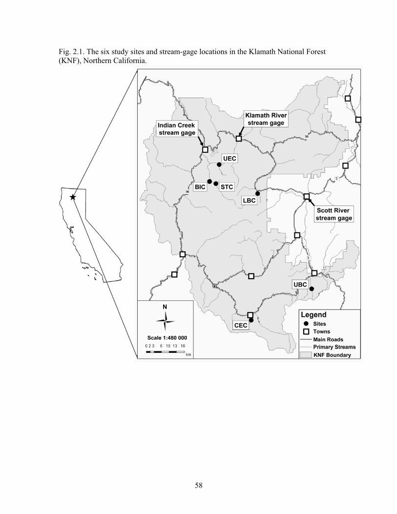
Fig. 2.1. The six study sites and stream-gage locations in the Klamath National Forest (KNF), Northern California.

58

Fig. 2.2 An example of (a) before and (b) after stream-crossing reconstruction from STC.

59

Fig. 2.3. Hydrographs from USGS stream gages in the region during the study period.

60

Fig. 2.4. An example of the sediment traps before (a) and after (b) stream crossing-reconstruction.

61

Fig. 2.5. Flow chart for the analysis of biological data from the targeted-riffle samples.

62

Fig. 2.6. The longitudinal profiles of the six sites the year prior to stream-crossing reconstruction (Y0-pre), just after reconstruction (Y0-post), one year after reconstruction (Y1), and two years after reconstruction (Y2).

63

Fig. 2.7. Channel-elevation change from the year prior to stream-crossing reconstruction (Y0-pre) to the second year after reconstruction (Y2) pooled for all the sites, with distance upstream (A) and downstream (B) of the stream crossings, determined using cross-sectional data.

64

Fig. 2.8. The first monumented upstream cross-section (XU2) at the six study sites, with post-construction (Y0-post) information only at sites where notable incision was evident.

65

Fig. 2.9. The first monumented downstream cross-section (XD2) at the six study sites.

66

Fig. 2.10. Riffle-surface fine-sediment upstream and downstream at the six sites with comparisons that had significant increases downstream highlighted with an asterisk.

67

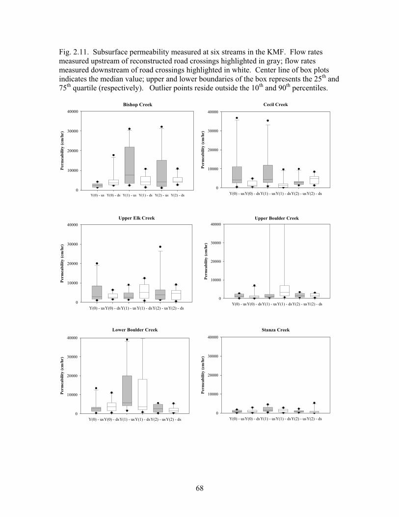
Fig. 2.11. Subsurface permeability measured at six streams in the KMF. Flow rates measured upstream of reconstructed road crossings highlighted in gray; flow rates measured downstream of road crossings highlighted in white. Center line of box plots indicates the median value; upper and lower boundaries of the box represents the 25th and 75th quartile (respectively). Outlier points reside outside the 10th and 90th percentiles.

Bishop Creek

Y(0) - us Y(0) - ds Y(1) - us Y(1) - ds Y(2) - us Y(2) - ds

Perm

eabi

lity

(cm

/hr)

0

10000

20000

30000

40000

Upper Boulder Creek

Y(0) - usY(0) - dsY(1) - usY(1) - dsY(2) - usY(2) - ds

Perm

eabi

lity

(cm

/hr)

0

10000

20000

30000

40000

Cecil Creek

Y(0) - usY(0) - dsY(1) - usY(1) - dsY(2) - usY(2) - ds

Perm

eabi

lity

(cm

/hr)

0

10000

20000

30000

40000

Stanza Creek

Y(0) - usY(0) - dsY(1) - usY(1) - dsY(2) - usY(2) - ds

Perm

eabi

lity

(cm

/hr)

0

10000

20000

30000

40000

Upper Elk Creek

Y(0) - usY(0) - dsY(1) - usY(1) - dsY(2) - usY(2) - ds

Perm

eabi

lity

(cm

/hr)

0

10000

20000

30000

40000

Lower Boulder Creek

Y(0) - usY(0) - dsY(1) - usY(1) - dsY(2) - usY(2) - ds

Perm

eabi

lity

(cm

/hr)

0

10000

20000

30000

40000

68

Fig. 2.12. The amount of sediment deposited in the sediment traps grouped by size.

69

Tabl

e 2.

1. S

ite lo

catio

ns a

nd d

escr

iptio

n of

act

iviti

es

Site

Cree

k Nam

e La

titud

e Lo

ngitu

de

Date

Sed

imen

t Tra

ps

Inst

alled

: Re

mov

ed

Com

plet

ion

Da

tePo

tent

ial M

igra

tion

Barri

er

Prio

r to

Reco

nstru

ctio

n (m

) Fi

ll Vol

ume R

emov

ed (m

3 )/ P

erce

nt R

emov

ed

BIC

Bish

op C

reek

41

°40'

12"

-123

°20'

60"

8/4/20

04 : 1

1/15/2

004

10/16

/2004

1.5

17

07 / 7

2%

CEC

Cecil

Cre

ek

41° 0

7' 12

" -1

23° 0

7' 48

" 7/2

8/200

4 : 8/

24/20

04

8/3/20

04

1.5

28 / 4

%

LBC

Lowe

r Bou

lder C

reek

41

° 37'

12"

-123

° 05'

60"

7/6/20

05 : 1

1/1/20

05

10/10

/2005

2.8

77

2 / 69

%

STC

Stan

za C

reek

41

° 40'

12"

-123

° 19'

12"

6/23/2

005 :

10/25

/2005

8/3

1/200

5 1.0

44

85 / 9

1%

UBC

Uppe

r Bou

lder C

reek

41

° 15'

00"

-122

° 48'

36"

8/19/2

004 :

11/3/

2004

10

/1/20

04

1.5

629 /

31%

UE

CUp

per E

lk Cr

eek

41° 4

4' 24

" -1

23° 1

7' 60

" 7/1

4/200

4 : 11

/9/20

04

10/21

/2004

1.5

43

78 / 9

9%

70

Table 2.2. Slopes of the longitudinal profiles overall, upstream (XU1-XU7), and downstream (XD1-XD5).

Site Year Overall Slope (%) Upstream Slope (%) Downstream Slope (%) BIC pre-Y0 5.6 4.6 5.9 post-Y0 5.7 4.8 6 Y1 5.5 5.1 6.2 Y2 5.7 5.7 5.7 CEC pre-Y0 6.4 6.5 7.1 post-Y0 6.4 6.7 7 Y1 6.5 6.9 7.5 Y2 6.4 7 7.5 STC pre-Y0 7.5 6.9 8.6 post-Y0 7.5 7 8.7 Y1 7.5 6.7 8.5 Y2 7.5 6.9 9.2 LBC pre-Y0 11.8 9.3 11.7 post-Y0 12 9 11.7 Y1 11.7 10.7 12.1 Y2 11.8 10.7 12.3 UBC pre-Y0 10.8 10 10.7 post-Y0 10.8 10.7 9.8 Y1 10.9 10.1 11 Y2 10.8 10.3 11 UEC pre-Y0 5.3 5 5.4 post-Y0 5.4 5.7 5 Y1 5.3 5.5 5.3 Y2 5.3 5.8 5.2

71

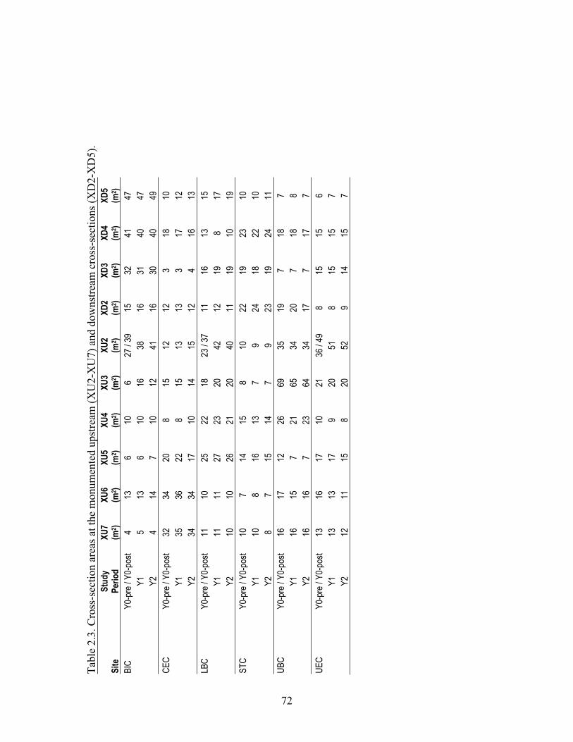
Tabl

e 2.

3. C

ross

-sec

tion

area

s at t

he m

onum

ente

d up

stre

am (X

U2-

XU

7) a

nd d

owns

tream

cro

ss-s

ectio

ns (X

D2-

XD

5).

Site

Stud

yPe

riod

XU7

(m2 )

XU6

(m2 )

XU5

(m2 )

XU4

(m2 )

XU3

(m2 )

XU2

(m2 )

XD2

(m2 )

XD3

(m2 )

XD4

(m2 )

XD5

(m2 )

BIC

Y0

-pre

/ Y0-

post

4 13

6

10

6 27

/ 39

15

32

41

47

Y1

5

13

6 10

16

38

16

31

40

47

Y2

4 14

7

10

12

41

16

30

40

49

CEC

Y0

-pre

/ Y0-

post

32

34

20

8 15

12

12

3

18

10

Y1

35

36

22

8

15

13

13

3 17

12

Y2

34

34

17

10

14

15

12

4 16

13

LB

C Y0

-pre

/ Y0-

post

11

10

25

22

18

23 / 3

7 11

16

13

15

Y1

11

11

27

23

20

42

12

19

8 17

Y2

10

10

26

21

20

40

11

19

10

19

STC

Y0-p

re / Y

0-po

st 10

7

14

15

8 10

22

19

23

10

Y1

10

8 16

13

7

9 24

18

22

10

Y2

8 7

15

14

7 9

23

19

24

11

UBC

Y0-p

re / Y

0-po

st 16

17

12

26

69

35

19

7

18

7

Y1

16

15

7 21

65

34

20

7

18

8

Y2

16

16

7 23

64

34

17

7

17

7 UE

C Y0

-pre

/ Y0-

post

13

16

17

10

21

36 / 4

9 8

15

15

6

Y1

13

13

17

9 20

51

8

15

15

7

Y2

12

11

15

8 20

52

9

14

15

7

72

Tabl

e 2.

4. P

ools

ups

tream

and

dow

nstre

am (U

S/D

S) o

f the

cul

verts

prio

r to

stre

am-c

ross

ing

reco

nstru

ctio

n (Y

0-pr

e), j

ust a

fter

reco

nstru

ctio

n (Y

0-po

st),

one

year

afte

r rec

onst

ruct

ion

(Y1)

, and

two

year

s afte

r rec

onst

ruct

ion

(Y2)

.

Befo

re R

econ

stru

ctio

n (Y

0-pr

e)

Just

Afte

r Rec

onst

ruct

ion

(Y0-

post

) On

e Yea

r Rec

onst

ruct

ion

(Y1)

Tw

o Ye

ars R

econ

stru

ctio

n (Y

2)

Site

Reac

hLe

ngth

(m)

Numb

er

of Pools

Ave.

Pool

Depth (m)

Max.D

epth

of

First

DSPo

ol (m

)

Numb

er

of Pools

Ave.

Pool

Depth (m)

Max.D

epth

of

First

DSPo

ol (m

)

Numb

er

of Pools

Ave.

Pool

Depth (m)

Max.D

epth

of

First

DSPo

ol (m

)

Numb

er

of Pools

Ave.

Pool

Depth (m)

Max.D

epth

of Fir

st DS

Po

ol (m

) BI

C 94

/ 79

1 / 2

0.80 /

0.83

1.2

0 0 /

2 --

/ 0.87

0.6

8 0 /

1 --

/ 0.74

0.9

1 0 /

1 --

/ 0.71

0.7

1 CE

C

143 /

102

2 / 3

0.69 /

0.70

1.2

3 1 /

1 0.5

4 / 0.

78

0.88

1 / 1

0.54 /

0.54

0.5

4 4 /

0 0.5

7 / --

--

UEC

11

9 / 88

4 /

2 0.6

7 / 0.

84

1.07

2 / 1

0.69 /

0.65

0.6

5 2 /

1 0.6

5 / 0.

59

0.61

3 / 3

0.60 /

0.61

0.5

3 UB

C

153 /

113

6 / 2

0.64 /

0.65

0.9

6 4 /

6 0.5

9 / 0.

58

0.51

2 / 3

0.62 /

0.60

0.6

2 /

4 0.6

4 / 0.

61

0.53

LBC

118 /

87

7 / 5

0.66 /

0.66

1.5

0 8 /

1 0.5

8 / 0.

51

0.51

5 / 4

0.69 /

0.59

0.5

1 4 /

2 0.5

7 / 0.

59

0.51

STC

98

/ 77

2 / 1

0.61 /

0.64

0.7

6 1 /

1 0.5

5 / 0.

68

0.68

2 / 0

0.74 /

--

-- 0 /

0 --

/ --

--

73

Tabl

e 2.

5. G

rain

-siz

e di

strib

utio

ns u

pstre

am a

nd d

owns

tream

of t

he st

ream

-cro

ssin

gs p

rior t

o st

ream

-cro

ssin

g re

cons

truct

ion

(Y0-

pre)

,on

e ye

ar a

fter r

econ

stru

ctio

n (Y

1), a

nd tw

o ye

ars a

fter r

econ

stru

ctio

n (Y

2).

D 16 (

mm

)

D 50 (

mm

)

D 84 (

mm

) Tr

eatm

ent

Site

Y0-p

re

Y1

Y2

Y0

-pre

Y1

Y2

Y0-p

re

Y1

Y2

Upstr

eam

BIC

8 6

5

67

82

64

31

3 44

2 36

5

CEC

6 4

4

128

113

134

46

0 38

5 47

6

UEC

4 4

5

91

66

90

45

7 37

1 46

4

UBC

5 <4

5

18

6 14

5 23

7

516

445

623

LB

C <4

5

4

123

252

157

49

8 58

5 52

0

STC

<4

<4

<4

50

69

61

354

299

407

Down

strea

m BI

C 8

<4

4

58

53

59

27

3 42

8 25

7

CEC

6 5

7

257

445

264

55

0 60

7 60

7

UEC

5 4

6

118

112

84

43

9 42

5 38

6

UBC

<4

4 4

16

4 11

7 16

6

554

408

542

LB

C <4

5

<4

10

4 17

8 11

4

370

459

478

ST

C <4

<4

<4

70

23

91

39

7 42

1 43

9

74

Tabl

e 2.

6. A

vera

ge m

ass o

f sed

imen

t dep

osite

d in

the

traps

ups

tream

and

dow

nstre

am o

f the

stre

am-c

ross

ings

at f

our s

ites (

SD in

pare

nthe

ses)

.

Aver

age M

ass o

f Sed

imen

t

Depo

sited

per

Sed

imen

t Tra

p (g

)

Site

Upstr

eam

Do

wnstr

eam

Perc

ent C

hang

e (U

pstre

am vs

Dow

nstre

am)

Num

ber o

f Sa

mpl

es (N

) Up

stre

am vs

. Dow

nstre

am

p-va

lue

(=0

.05)

BIC

11.47

(6.39

)

97.01

(21.1

1)

74

5%

5

p =

<0.0

01

CEC

6.4

4 (6.0

7)

38

.59 (1

2.32)

499%

5

p = <

0.001

UE

C 36

.10 (8

.86)

17

9.92 (

46.69

)

398%

4

p = <

0.001

UB

C 93

.80 (4

2.44)

847.6

9 (26

3.38)

804%

5

p = <

0.001

75

Tabl

e 2.

7. M

etric

s with

pre

dict

ed d

irect

iona

l res

pons

e an

d th

e su

m o

f com

paris

ons b

etw

een

the

year

prio

r to

(Y0-

pre)

and

the

year

af

ter (

Y1)

stre

am-c

ross

ing

reco

nstru

ctio

n, th

e ye

ar p

rior t

o (Y

0-pr

e) a

nd th

e se

cond

yea

r afte

r (Y

2), a

nd th

e ye

ar a

fter (

Y1)

and

the

seco

nd y

ear a

fter (

Y2)

.

Metri

cRi

chne

ss

Abun

danc

e

Sim

pson

's Di

vers

ity

Inde

x

# of H

BI

Into

leran

t

# of H

BI

Toler

ant

Pred

icted

dire

ction

De

creas

e De

creas

eDe

creas

eDe

creas

eInc

reas

e

US

DS

US

DS

US

DS

US

DS

US

DS

# o

f com

paris

ons

18

18

18

18

18

18

18

18

18

18

# o

f CVs

> na

tural

varia

bility

2

3

8

11

9

14

10

15

13

14

#

going

in pr

edict

ed di

recti

on

0

1 3

6

2

5 7

8

5

9 # o

f CVs

> 1/

2 natu

ral v

ariab

ility

7

10

13

14

13

18

12

17

13

14

#

going

in pr

edict

ed di

recti

on

2

4 3

6

6

8 9

10

5

9

Metri

c# o

f Eph

emer

opte

ra

Taxa

Ep

hem

erop

tera

Ab

unda

nce

# o

f Tric

hopt

era

Taxa

Tr

ichop

tera

Ab

unda

nce

# o

f Plec

opte

ra

Taxa

Pred

icted

dire

ction

De

creas

e De

creas

eDe

creas

eDe

creas

eDe

creas

e

US

DS

US

DS

US

DS

US

DS

US

DS

# o

f com

paris

ons

18

18

18

18

18

18

18

18

18

18

# o

f CVs

> na

tural

varia

bility

2

2

10

16

1

6

9

15

2

3

# go

ing in

pred

icted

dire

ction

0

1

3

6 0

3

4

7 0

1

# of C

Vs >

1/2 n

atura

l var

iabilit

y 3

6

13

18

5

9

14

17

6

7

#

going

in pr

edict

ed di

recti

on

0

3 6

7

3

3 8

8

1

3

Me

tric

Plec

opte

raAb

unda

nce

%

EPT

EPT

Ab

unda

nce

EP

T

Rich

ness

Pred

icted

dire

ction

De

creas

e De

creas

eDe

creas

eDe

creas

e

US

DS

US

DS

US

DS

US

DS

# of c

ompa

rison

s 18

18

18

18

18

18

18

18

# o

f CVs

> na

tural

varia

bility

10

12

7

10

8

15

2

5

# go

ing in

pred

icted

dire

ction

2

5

1

5 4

7

0

3 # o

f CVs

> 1/

2 natu

ral v

ariab

ility

15

17

12

13

12

16

6

9

#

going

in pr

edict

ed di

recti

on

7

8 5

7

4

7 2

5

76

Tabl

e 2.

8. C

umul

ativ

e nu

mbe

r of c

ompa

rison

s am

ong

all t

he m

etric

s tha

t sho

wed

cha

nges

out

side

the

rang

e of

exp

ecte

d na

tura

l va

riabi

lity

in th

e di

rect

ion

mos

t lik

ely

to re

flect

an

impa

ct a

ssoc

iate

d w

ith e

leva

ted

leve

ls o

f fin

e-se

dim

ent i

n th

e ch

anne

l.

Perio

d

# of c

ompa

rison

s > n

atur

al CV

Sign

ifica

nce

# o

f com

paris

ons >

1/2 n

atur

al CV

Sign

ifica

nce

Upstr

eam

Down

strea

m

= 0.

05

Up

strea

m Do

wnstr

eam

=

0.05

Y0

-pre

- Y1

9 (1.8

) 27

(4.0)

P =

<0.00

1

19 (1

.9)

40 (4

.0)

P

= <0

.001

Y0-p

re -

Y2

12

(2.4)

23

(2.3)

P =

<0.00

1

23 (2

.3)

32 (1

.2)

P

= <0

.001

Y1 -

Y2

10

(2.7)

16

(1.6)

P =

<0.00

1

23 (2

.9)

22 (2

.4)

P

= 0.3

83

77

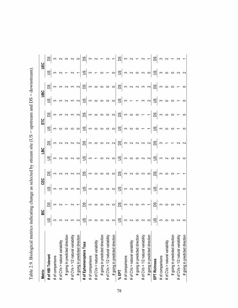
Tabl

e 2.

9. B

iolo

gica

l met

rics i

ndic

atin

g ch

ange

as s

elec

ted

by st

ream

site

(US

= up

stre

am a

nd D

S =

dow

nstre

am).

Metri

cBI

C

CEC

LB

C

STC

UB

C

UEC

# of H

BI T

oler

ant

US

DS

US

DS

US

DS

US

DS

US

DS

US

DS

# of c

ompa

rison

s

3

3

3

3

3

3

3

3

3

3

3

3 # o

f CVs

> na

tural

varia

bility

3

2

3

2

2

2

0

3

3

3

2

2

# go

ing in

pred

icted

dire

ction

2

1

0

2

0

2

0

2

2

2

1

0 # o

f CVs

> 1/

2 natu

ral v

ariab

ility

3

2

3

2

2

2

0

3

3

3

2

2

#

going

in pr

edict

ed di

recti

on

2

1

0

2

0

2

0

2

2

2

1

0

# of E

phem

erop

tera

Tax

a

US

DS

US

DS

US

DS

US

DS

US

DS

US

DS

# o

f com

paris

ons

3

3

3

3

3

3

3

3

3

3

3

3

# of C

Vs >

natur

al va

riabil

ity

0

0

0

0

1

0

0

0

0

0

1

2

#

going

in pr

edict

ed di

recti

on

0

0

0

0

0

0

0

0

0

0

0

1

# of C

Vs >

1/2 n

atura

l var

iabilit

y

0

2

0

0

2

2

0

0

0

0

1

2

# go

ing in

pred

icted

dire

ction

0

0

0

0

0

2

0

0

0

0

0

1 %

EPT

US

DS

US

DS

US

DS

US

DS

US

DS

US

DS

# o

f com

paris

ons

3

3

3

3

3

3

3

3

3

3

3

3

# of C

Vs >

natur

al va

riabil

ity

2

2

2

2

0

2

0

0

1

2

2

2

#

going

in pr

edict

ed di

recti

on

0

0

0

0

0

2

0

0

1

2

0

1

# of C

Vs >

1/2 n

atura

l var

iabilit

y

2

3

2

2

2

2

1

1

3

3

2

2

# go

ing in

pred

icted

dire

ction

0

1

0

0

2

2

1

1

2

2

0

1 EP

T Ri

chne

ss

US

DS

US

DS

US

DS

US

DS

US

DS

US

DS

# of c

ompa

rison

s

3

3

3

3

3

3

3

3

3

3

3

3 # o

f CVs

> na

tural

varia

bility

0

0

0

0

2

1

0

0

0

0

0

2

# go

ing in

pred

icted

dire

ction

0

0

0

0

0

1

0

0

0

0

0

1 # o

f CVs

> 1/

2 natu

ral v

ariab

ility

2

2

0

1

2

2

1

1

1

1

2

2

#

going

in pr

edict

ed di

recti

on

0

1

0

1

0

2

0

0

0

0

2

1

78

Tabl

e 2.

10. T

en se

dim

ent s

ensi

tive

taxa

indi

catin

g ch

ange

in a

bund

ance

as s

elec

ted

by st

ream

site

ups

tream

(US)

and

dow

nstre

am

(DS)

.Ta

xaAn

toch

asp

p.At

tene

lla

delan

tala

Chiro

no-

min

aeDi

cran

ota

spp.

Drun

ella

dodd

siDr

unell

asp

inife

ra

Eccli

som

yiasp

p.Ep

eoru

ssp

p.Ol

igo-

chae

taZa

pada

co

lum

bian

a Pr

edict

ed D

irecti

on

De

crea

se

Incr

ease

De

crea

se

Decr

ease

De

crea

se

Decr

ease

De

crea

se

Decr

ease

In

crea

se

Incr

ease

BI

C Y0

-pre

0 /

0 0 /

0 33

3 / 19

32

/ 0

32 / 3

0 /

0 0 /

0 17

/ 15

0 / 1

0 / 0

US / D

S Y1

22

/ 16

0 / 0

16 / 1

9 0 /

0 11

/ 16

0 / 0

0 / 0

32 / 1

02

0 / 0

102 /

0

Y2

0 / 0

0 / 0

100 /

46

0 / 0

14 / 9

0 /

0 0 /

0 57

/ 15

0 / 0

7 / 0

CEC

Y0

0 / 16

0 /

0 19

4 / 24

7 93

/ 1

452 /

66

0 / 0

0 / 0

43 / 2

2 0 /

0 47

3 / 26

9 US

/ DS

Y1

27 / 1

6 0 /

0 99

7 / 44

1 13

/ 5

134 /

215

0 / 22

0 /

0 55

/ 70

0 / 0

0 /

0

Y2

6 / 10

5 0 /

0 10

1 / 38

7 8 /

9 71

/ 163

0 /

0 0 /

0 25

/ 86

12 / 0

18

/ 0

LBC

Y0-p

re

0 / 0

0 / 0

11 / 4

3 0 /

34

55 / 0

5 /

4 0 /

0 10

69 / 1

81

0 / 0

0 / 0

US / D

S Y1

0 /

0 0 /

0 14

6 / 46

10

/ 3

258 /

341

13 / 8

0 /

0 23

7 / 10

8 0 /

0 43

9 / 0

Y2

43

/ 0

0 / 0

4688

/ 111

9 12

9 / 0

1935

/ 447

12

9 / 17

0 /

0 86

0 / 86

2 0 /

191

7747

/ 141

1 ST

C Y0

-pre

0 /

0 0 /

0 17

7 / 22

0 /

0 11

/ 5

0 / 0

0 / 0

89 / 9

7 0 /

0 0 /

0 US

/ DS

Y1

11 / 5

0 /

32

11 / 1

1 5 /

5 5 /

16

0 / 0

0 / 0

22 / 8

1 0 /

0 0 /

11

Y2

0 /

0 0 /

0 31

/ 24

6 / 5

6 / 0

0 / 0

0 / 0

143 /

122

0 / 0

289 /

19

UBC

Y0-p

re

0 / 0

0 / 0

9 / 57

0 /

0 77

/ 315

0 /

0 0 /

0 13

60 / 6

63

0 / 43

17

/ 0

US / D

S Y1

0 /

0 0 /

0 86

/ 11

0 / 0

172 /

187

0 / 0

0 / 0

269 /

429

0 / 0

0 / 5

Y2

12

/ 32

0 / 0

36 / 6

5 5 /

0 55

/ 108

12

/ 22

0 / 0

153 /

667

0 / 16

1 12

/ 11

UEC

Y0-p

re

0 / 9

0 / 0

8 / 12

21

5 / 17

19

/ 576

0 /

0 0 /

0 59

/ 153

0 /

0 3 /

0 US

/ DS

Y1

22 / 1

0 0 /

0 65

/ 129

0 /

0 11

/ 0

0 / 0

0 / 0

0 / 5

0 / 0

0 / 0

Y2

0 /

0 0 /

0 22

/ 17

0 / 0

86 / 3

3 0 /

0 0 /

0 26

5 / 64

7 /

0 0 /

0

79

Tabl

e 2.

11. A

bund

ance

s of d

omin

ant E

PT ta

xa c

olle

cted

in th

e co

loni

zatio

n tra

ps u

pstre

am a

nd d

owns

tream

of t

he st

ream

cro

ssin

gs.

EPT

Taxa

Up

stre

am A

bund

ance

Do

wnst

ream

Abu

ndan

ce

Lepid

ostom

atida

e 1,3

56

121

Chlor

oper

lidae

65

0 36

3 Le

ptoph

lebiid

ae

425

146

Amele

tus sp

.

27

7 74

He

ptage

niida

e 21

1 29

Lim

neph

ilidae

11

1 57

Ba

etida

e 13

4 23

Rh

yaco

philid

ae

56

65

80

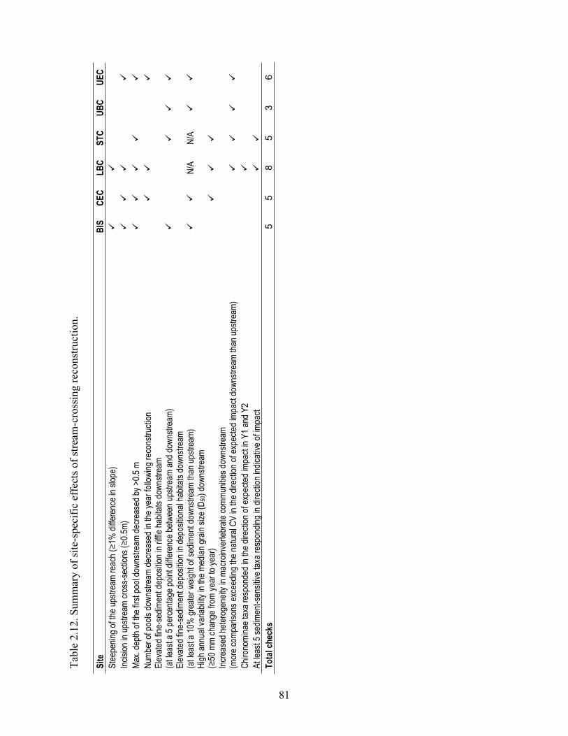
Tabl

e 2.

12. S

umm

ary

of si

te-s

peci

fic e

ffec

ts o

f stre

am-c

ross

ing

reco

nstru

ctio

n.

Site

BIS

CEC

LBC

STC

UBC

UEC

Stee

penin

g of th

e ups

tream

reac

h (1%

diffe

renc

e in s

lope)

Inc

ision

in up

strea

m cro

ss-se

ction

s (0.5

m)Ma

x. de

pth of

the f

irst p

ool d

owns

tream

decre

ased

by >

0.5 m

Nu

mber

of po

ols do

wnstr

eam

decre

ased

in th

e yea

r foll

owing

reco

nstru

ction

Elev

ated f

ine-se

dimen

t dep

ositio

n in r

iffle h

abita

ts do

wnstr

eam

(a

t leas

t a 5

perce

ntage

point

diffe

renc

e betw

een u

pstre

am an

d dow

nstre

am)

Elev

ated f

ine-se

dimen

t dep

ositio

n in d

epos

itiona

l hab

itats

down

strea

m (a

t leas

t a 10

% gr

eater

weig

ht of

sedim

ent d

owns

tream

than

upstr

eam)

N/A

N/A

High

annu

al va

riabil

ity in

the m

edian

grain

size

(D50

) dow

nstre

am

(50

mm

chan

ge fr

om ye

ar to

year

) Inc

reas

ed he

terog

eneit

y in m

acro

inver

tebra

te co

mmun

ities d

owns

tream

(mor

e com

paris

ons e

xcee

ding t

he na

tural

CV in

the d

irecti

on of

expe

cted i

mpac

t dow

nstre

am th

an up

strea

m)

Chiro

nomi

nae t

axa r

espo

nded

in th

e dire

ction

of ex

pecte

d imp

act in

Y1 a

nd Y

2 At

leas

t 5 se

dimen

t-sen

sitive

taxa

resp

ondin

g in d

irecti

on in

dicati

ve of

impa

ct To

tal c

heck

s 5

5 8

5 3

6

81

CHAPTER 3

The effects of vineyard coverage and extent on benthic macroinvertebrates in mediterranean-climate streams of Northern California

82

The effects of vineyard coverage and extent on benthic macroinvertebrates in mediterranean-climate streams of Northern California

Abstract

Vineyards are a dominant feature of many landscapes in Mediterranean-climate regions. I examined the effects of streamflow declines, associated with vineyard water withdrawals for frost protection, on benthic-macroinvertebrate communities at three sites along three small streams in the Mediterranean-climate region of Northern California. One site was heavily impacted by water withdrawals for frost protection, the other two were not. In addition, I examined relationships between vineyard coverage and benthic-macroinvertebrate community response using data collected from 59 sites along 35 small streams in Lake, Napa, and Sonoma Counties, California. I tested three a priorihypotheses concerning the response of biological traits of macroinvertebrates to high vineyard coverage: 1) semi-voltine (i.e., one generation every two years) individuals would decline (compared to uni- and multi-voltine individuals), 2) individuals with the ability to undergo diapause would increase, and 3) individuals with the ability to burrow into the substrate would increase. In the site-specific study, I found that vineyard water withdrawals for frost protection coincided with consistent declines both in the benthic macroinvertebrate index of biotic integrity (B-IBI) developed for Northern California streams and the ratio of Ephemeroptera-Plectoptera-Trichoptera to Odonata-Coleoptera-Hemiptera individuals (EPT/OCH), a metric developed for European Mediterranean streams. In the broader-scale study, I observed that vineyard coverage levels above a ~20% threshold coincided with lower values of the B-IBI. The semi-voltine life-cycle trait declined above this threshold, whereas the diapause and burrowing traits were not affected.

Key words: vineyards; frost protection; benthic macroinvertebrates; biological monitoring; threshold effects

83

Introduction

The growing of grapes for wine has been done in Mediterranean-climate regions for millennia. However, grape vines in these regions are susceptible to tissue damage when air temperatures are low. In northern-hemisphere, Mediterranean-climate regions, low-temperature injuries most commonly occur in spring months, during the period of bud development, when air temperatures drop below -0.5ºC (Kasimatis et al. 1974). There are several methods that vineyards use for frost protection in the spring, including vineyard-site selection, grape-variety selection, cultural practices, wind circulation, heaters, and water sprinklers (Kasimatis and Kissler 1974, Johnson and Howell 1981, Donaldson et al. 1993). Approximately 9% of the total irrigated vineyard land in California has water-sprinker systems installed (Orang et al. 2008). The use of sprinker systems for frost protection has been observed repeatedly to drastically reduce streamflow in small streams in the Mediterranean-climate region of northern California (Deitch et al. 2009). These reductions typically occur between the months of March and April (Deitch et al. 2009), which coincides with the end of the rainy season in this region (Gasith and Resh 1999). This is a very important period of time for benthic macroinvertebrates because this is when the majority of pre-emergence growth occurs (Mendez and Resh 2008). The effects of reductions in streamflow associated with vineyard water withdrawals for frost protection on the abundance and composition of benthic-macroinvertebrate communities have not been explored in other studies. However, many studies have shown a strong relationship between streamflow reductions and benthic-macroinvertebrate response in Mediterranean-climate streams (e.g., Acuña et al. 2005, Bonada et al. 2006, 2007, Álvarez and Pardo 2009). Furthermore, prolonged drought in Mediterranean-climate regions extending over multiple years has particularly strong effects on the abundance and composition of benthic macroinvertebrate communities in small streams (Bêche et al. 2006, Bêche and Resh 2007a,b). Water diversions during these drought periods increase the impacts on these benthic communities (Gasith and Resh 1999). Streamflow reductions associated with frost protection could also have a selective effect on biological traits of benthic-macroinvertebrate communities. The traits for a given taxon may include, for example, the number of generations per year, the ability to enter a state of diapause, and the ability to burrow into the streambed to obtain food, seek refuge from predators, or escape low-flow conditions (Bêche and Resh 2007a,b).Biological traits of benthic-macroinvertebrate communities in Mediterranean-climate regions have been shown to be affected by long-term climate variability (Bêche et al. 2006; Bêche and Resh 2007a,b) and seasonal differences in climate (Mouthon and Daufresne 2006, Cordellier and Pfenninger 2008, Spooner and Vaughn 2008, Clausnitzer et al. 2009, Hering et al. 2009). The objectives of this study are to determine whether: 1) vineyard water withdrawals for frost protection affect benthic-macroinvertebrate communities; 2) whether there is a threshold of vineyard coverage above which the effects are more pronounced; and 3) whether exceeding this threshold has any effect on a priori selected biological traits. These questions have implications for evaluating the effects of vineyard coverage on streams in Northern California and potentially in wine-producing areas in

84

other Mediterranean-climate regions around the world. These areas occur in parts of Europe around the Mediterranean Sea, Southern California, South Africa, Australia, and Chile (Gasith and Resh 1999).

Methods

Study sites and benthic macroinvertebrate data This study is based on two benthic macroinvertebrate datasets from the wine-producing region of Northern California. The first dataset includes benthic macroinvertebrate samples collected intensively over time. It is used to examine change in benthic-macroinvertebrate communities occurring over two years (2004 - 2005) in three sites along three small streams (Franz Creek, Bidwell Creek, and Maacama Creek; Fig. 3.1) in Sonoma County, California, just before, during, and just after the period of water withdrawal for frost-protection. The watershed areas of these sites ranged from 13 to 106 km2 and the vineyard coverage upstream of the sites ranged from 6 to 14 % of the watershed area. Depending on the year, this frost-protection period can occur anytime from mid-February to mid-May in Northern California (Smith et al. 2004). The effect of water withdrawals for vineyard frost-protection on streamflow differed among the three streams examined (Deitch et al. 2009). For example, the reduction in streamflow was greater than 75% in Franz Creek on six occasions over the two years of the study, whereas the reduction in streamflow never surpassed this 75%-threshold in either of the other two streams examined (Deitch et al. 2009). The highest magnitude changes in streamflow associated with a single frost-protection event were 530 L/s in Franz Creek and 120 L/s in Bidwell Creek (Deitch et al. 2009). The highest magnitude change in streamflow associated with a single event at Maacama Creek was lower than at both Franz Creek and Bidwell Creek, but the exact amount is unknown because the vineyards in the watershed above Maacama Creek are located farther from the sampling site and, as a result, the change in streamflow was extended over a long time-span (Deitch et al. 2009).

Benthic macroinvertebrates were sampled at the three sites from a fixed area of 0.09 m2 in individual riffles using a D-frame kicknet with a mesh size of 500 μm. Sampling began in early March and extended into early May each year, and included one sample per event. All taxa in these samples were indentified to genus level. Vineyard water withdrawals for frost protection at these sites began in mid-March and extended into mid-April each year during this study (see Deitch et al. (2009) for the dates, magnitude, and duration of the associated streamflow declines).

The second dataset contains samples collected intensively over space. It is used to examine differences in benthic-macroinvertebrate communities among 59 sites along 35 streams in Lake, Napa, and Sonoma Counties, California (Fig. 3.1). These sites had different levels of vineyard coverage in the watershed upstream of each site (described as % of land-cover). The watershed areas of these sites ranged from one to 209 km2 and the vineyard coverage ranged from zero to 76%. Benthic macroinvertebrate samples were collected by the Friends of the Napa River over a two year period (2000-2001) as part of a locally organized biomonitoring effort. Collections were made in mid-April following the standard, targeted-riffle approach of the California SWAMP bioassessment protocol (Ode 2007). Three replicates

85

were collected, each taken from a fixed area of 1.8 m2 using a net with a mesh size of 500 μm. All taxa in these samples were identified to genus level by Aquatic Biology Associates, Inc., Corvallis, Oregon.

Evaluating the effects of vineyard water withdrawals for frost protection I calculated five biological metrics from the data, including the North Coast B-IBI (Rehn et al. 2005), total taxa richness, total abundance, % EPT individuals, and EPT / OCH richness, an index proposed for Mediterranean-climate streams by Bonada et al. (2006). The North Coast B-IBI is composed of eight metrics, which include EPT richness, Coleoptera richness, Diptera richness, % intolerant individuals, % non-Gastropoda scraper individuals, % predator individuals, % shredder taxa, and % non-insect taxa (Rehn et al. 2005). I calculated values for these metrics from samples collected just before water withdrawals for frost protection occurred (early March) and just after (late June), and examined the change in the metric values separately for each year. To determine whether there is a vineyard-coverage threshold above which the effects of vineyards are more pronounced, I calculated values of the North Coast B-IBI for all of the sampling events in the 59 sites and examined the values across the range of vineyard densities. I first plotted these B-IBI values against percent-vineyard coverage to select an arbitrary threshold. I then calculated the average, range, and the standard deviation of the final B-IBI values above and below the selected vineyard-coverage threshold, and did the same for each of the eight component metrics of the B-IBI. To determine whether the threshold was statistically significant, I compared the metric values above and below the threshold using Student's t-tests. The a priori hypothesis was that the average value of the B-IBI would be higher for sites below the threshold than for those above the threshold because the B-IBI was designed to detect land-use effects by reflecting higher levels of disturbance with lower B-IBI values (Rehn et al. 2005).

The effects of vineyard coverage on biological traits Three biological traits of benthic macroinvertebrates (voltinism, resistance to desiccation, and locomotion abilities) were examined because they were hypothesized apriori to be responsive to streamflow reductions based on their functional attributes (Bêche et al. 2006). I focused on specific categories within these traits including the presence of a semi-voltine (i.e., two generations per year compared to the one generation per year of the uni-voltine and many generations of the multi-voltine) life cycle, diapause (i.e., the ability to enter a period of suspended growth and development in response to environmental stress), and burrowing ability (i.e., taxa that can dig down into the stream bottom to find food, refuge from predators, and shelter during low streamflow) because these traits would likely show a response to the effects of the streamflow reductions associated with vineyard water withdrawals. The a priori hypotheses were that above the vineyard-coverage threshold 1) there would be a decrease in semi-voltine (i.e., long-lived) taxa, 2) there would be an increase in taxa that undergo diapause, and 3) there would be an increase in taxa that burrow into the substrate. The distribution of biological traits among taxa was calculated using abundance data. The traits for all taxa present in each sample and the proportional representation of each trait category were determined based on the descriptions used by Bêche et al.

86

(2006). Because the fuzzy-coding approach was used (Chevenet et al. 1994), each taxon could be described by a fractional composition of multiple trait categories, e.g., a taxon could be described as 0.4 semi-voltine and 0.6 bi-voltine, with the fractions summing to one, which would indicate that this taxon has partial semi-voltine and partial bi-voltine characteristics.

Results

The effects of vineyard water-withdrawals for frost protection The two-year study conducted at three sites revealed a decrease in the value of the North Coast B-IBI and in the ratio of EPT to OCH individuals in the stream most impacted by water withdrawals for frost protection (Franz Creek) during the three-month frost-protection period in both years of the study (Table 3.1). However, there was variability in metric values within this time-span (Fig. 3.2). In one of the other streams (Bidwell Creek), the value of the B-IBI consistently increased during this time-span in both years, and in the other stream (Maacama Creek) there was no consistent trend (Table 1). In neither Bidwell Creek nor Maacama Creek, were there any consistent trends in the ratio of EPT to OCH individuals during this time-span (Table 3.1).

The determination of a vineyard-coverage threshold There was a clear effect of vineyards on benthic macroinvertebrates above a threshold of ~20% vineyard coverage (Fig. 3.3). The difference in the average value of the B-IBI below and above this threshold was statistically significant (Table 3.2). Of the eight component metrics of the B-IBI, six indicated a significant difference above and below the 20% threshold when examined independently; these included EPT richness, Coleoptera richness, Diptera richness, % intolerant individuals, % non-gastropoda scraper individuals, and % non-insect taxa (Table 2). The two component metrics that did not indicate a significant difference were % predator individuals and % shredder taxa (Table 3.2). However, the statistical power ( ) was less than the desired level of 0.8 for the comparisons involving these two metrics as a result of the small effect size (Table 3.2).

The effects of vineyard coverage on biological traits There was some evidence for the occurrence of a lower percentage of individuals with the semivoltine life-cycle trait above the 20% threshold (Fig. 3.4). For example, the percentage of individuals with this life-cycle ranged from 0 to 37 % with a mean of 11% below the threshold and from 0 to 10 % with a mean of 3 % above the threshold. The difference between these mean values was significant (P < 0.03). However, there was no evidence for a threshold effect on the diapause and burrowing traits.

Discussion

The biological effect that was observed in Franz Creek, the stream where the largest proportional reductions in streamflow occurred as a result of vineyard water withdrawals for frost protection (Fig. 3.2), is within the range for which the B-IBI was designed to detect (Rehn et al. 2005). It is highly likely that this effect was related to the water withdrawals for frost protection because a consistent decrease in the B-IBI was not

87

observed in either of the other two streams where flow-reduction effects were much lower (Table 3.1). Likewise, the decrease in the EPT to OCH ratio in Franz Creek indicates that the stream system is shifting to a state that is increasingly dominated by pools as opposed to riffles (Bonada et al. 2006), which is consistent with the direction one would expect to be associated with a reduction in streamflow. A consistent decrease in the EPT to OCH ratio was not observed in the other two sites during the frost-protection period, which provides further evidence that vineyard water withdrawals for frost-protection are causing the effect. The 20% vineyard-coverage threshold that was evident from the B-IBI (Table 3.2, Fig. 3.3) represents the level of vineyard development above which a strong effect can be expected on benthic communities. The maximum value of the B-IBI above the threshold was 23 points lower than the maximum value below the threshold. None of the sites above the threshold had a B-IBI value indicative of "good" conditions according to Rehn et al. (2005), i.e., B-IBI value greater than 61, whereas 41% of the sites below the threshold did. The percent shredders may have remained fairly constant across different levels of vineyard coverage because riparian corridors are maintained along streams in this region (Nicholls et al. 2001) and these corridors may provide consistent litter input from trees that could supply a food source for shredders. The percent predators may have remained constant because the predators could shift to a different prey as the community composition changed in response to different levels of vineyard development. The decrease in semi-voltine (i.e., long-lived) individuals above the 20% threshold (Fig. 3.4) may relate to higher predation pressure or intolerance of lower flow and perhaps oxygen levels as a result of the sudden reductions in streamflow. These individuals would not be able to replenish their populations as quickly as individuals with shorter life-spans after these water-withdrawal episodes. The absence of a response in individuals with the trait that allows them to enter a diapause stage when exposed to unfavorable conditions may relate to the short duration of the streamflow declines, which may not have been long enough to trigger diapause and thereby confer a selective advantage. Furthermore, the absence of a response in burrowing individuals could relate to the presence of disconnected pools, which provide sufficient refuge during the streamflow declines to support individuals with other locomotive traits, such as the ability to fly, swim, and/or crawl. An effect of extensive water withdrawals associated with high vineyard coverage on benthic macroinvertebrates in the Mediterranean-climate region of Northern California is clearly evident from this study. A combination of this water-withdrawal practice coupled with other factors, such as fertilizer and pesticide use, and/or increased erosion and sedimentation as a result of tillage, may impact benthic macroinvertebrate communities and consequently their availability as food for higher trophic levels such as amphibians, fish, and birds. The impact of vineyards in the Mediterranean-climate region of Northern California may be particularly intense relative to other Mediterranean-climate regions around the world because the viticulture system in California is more of a monoculture than the systems in other Mediterranean, wine-growing regions, such as parts of Portugal and Spain, where the systems are characterized by small, family-owned farms (Altieri and Nicholls 2002). Determination of whether these threshold effects also apply to benthic macroinveretbrates in these regions may be a useful tool for management of riverine habitats and water withdrawal schemes in these areas.

88

Acknowledgements

I thank M. Matella for her assistance with vineyard-coverage calculations and L. Bêche for providing information on biological traits for specific genera. I also thank the US Department of Agriculture Forest Service under Cost Share Agreement #03-CR-11052007–042, the Edward A. Colman Fellowship in Watershed Management from the Department of Environmental Science, Policy, and Management at UC Berkeley, and the Pinto-Fialon Endowment administered by the Portuguese Studies Program (PSP) at UC Berkeley for support.

Literature Cited Altieri, M.A. and Nicholls, C.I. 2002. The Simplification of Traditional Vineyard Based Agroforests in Northwestern Portugal: Some Ecological Implications. Agroforestry Systems 56: 185-191.

Acuña, V., Muñoz, I., Giorgi A., Omella, M., Sabater, F., and S. Sabater. 2005. Drought and postdrought recovery cycles in an intermittent Mediterranean stream: structural and functional aspects. Journal of the North American Benthological Society 24: 919-933.

Álvarez, M. and I. Pardo 2009. Dynamics in the trophic structure of the macroinvertebrate community in a Mediterranean, temporary stream. Aquatic Sciences - Research Across Boundaries 71: 202-213.

Bêche, L. A., E. P. McElravy, and V. H. Resh. 2006. Long-term seasonal variation in the biological traits of benthic macroinvertebrates in two Mediterranean-climate streams. Freshwater Biology 51: 56-75.

Bêche, L.A., and V. H. Resh. 2007a. Biological traits of benthic macroinvertebrates in California mediterranean-climate streams: Long-term annual variability and trait diversity patterns. Fundamental and Applied Limnology 161: 1-23.

Bêche, L. A., and V. H. Resh. 2007b. Short-term climatic trends affect the temporal variability of macroinvertebrates in California 'mediterranean' streams. Freshwater Biology 52: 2317-2339.

Bonada, N., M. Rieradevall, N. Prat, and V. H. Resh. 2006. Benthic macroinvertebrate assemblages and macrohabitat connectivity in Mediterranean-climate streams of northern California. Journal of the North American Benthological Society 25: 32-43.

Bonada, N., Rieradevall, M., and N. Prat. 2007. Macroinvertebrate community structure and biological traits related to flow permanence in a Mediterranean river network. Hydrobiologia 589: 91-106.

89

California Department of Fish and Game (DFG). 2003. California stream bioassessment procedure. Technical Report. California Aquatic Bioassessment Laboratory, Sacramento, CA.

Clausnitzer V., V. J. Kalkman, M. Ramc, B. Collen, J. E. M. Baillie, M. Bedjani , W. R. T. Darwall, K. D. B. Dijkstra, R. Dow, J. Hawking, H. Karube, E. Malikova, D. Paulson, K. Schütte, F. Suhling, R. J. Villanueva, N. von Ellenrieder, and K. Wilson 2009. Odonata enter the biodiversity crisis debate: The first global assessment of an insect group. Biological Conservation 142: 1864-1869.

Cordellier, M., and M. Pfenninger. 2008. Climate-driven range dynamics of the freshwater limpet, Ancylus fluviatilis (Pulmonata, Basommatophora). Journal of Biogeography 35: 1580-1592.

Deitch, M. J., Kondolf, G. M., and A. M. Merenlender. 2010. Hydrologic impacts of small-scale instream diversions for frost and heat protection in the California Wine Country. River Research and Applications 25: 118-134.

Donaldson, D. R., R. L. Snyder, C. Elmore, and S. Gallagher. 1993. Weed control influences vineyard minimum temperatures. American Journal of Enology and Viticulture 44: 431-434.

Gasith, A., and V. H. Resh. 1999. Streams in Mediterranean climate regions: Abiotic influences and biotic responses to predictable seasonal events. Annual Review of Ecology and Systematics 30: 51-81.

Hering, D., A. Schmidth-Kloiber, J. Murphy, S. Lücke, C. Zamora-Muñoz, M. J. López-Rodríguez, T. Huber, and W. Graf. 2009. Potential impact of climate change on aquatic insects: A sensitivity analysis for European caddisflies (Trichoptera) based on distribution patterns and ecological preferences. Aquatic Sciences - Research Across Boundaries 71: 3-14.

Johnson, D. E., and G. S. Howell. 1981. Factors influencing critical temperatures for spring freeze damage to developing primary shoots on Concord grapevines. American Journal of Enology and Viticulture 32: 144-149.

Kasimatis, A. N., and J. J. Kissler.1974. Responses of grapevines to shoot break-out following injury by spring frost. American Journal of Enology and Viticulture 25:17-20.

Mouthon, J., and M. Daufresne. 2006. Effects of the 2003 heatwave and climatic warming on mollusc communities of the Saône: a large lowland river and of its two main tributaries (France). Global Change Biology 12: 441–449.

Nicholls, C. I., Parrella, M., and M. A. Altieri. 2001. The effects of a vegetational corridor on the abundance and dispersal of insect biodiversity within a northern California organic vineyard. Landscape Ecology 16: 133-146.

90

Orang, M. N., Matyac, J. S., and Snyder, R. L. 2008. Survey of irrigation methods in California in 2001. Journal of Irrigation and Drain Engineering 134: 96-100.

Rehn, A. C., P. R. Ode, and J. T. May. 2005. Development of a benthic index of biotic integrity (B- IBI) for wadeable streams in northern coastal California and its application to regional 305(b) reporting. California State Water Quality Control Board, Sacramento, California.

Smith R.J., Klonsky K. M., Livingston P. L., and DeMoura, R.L. 2004. sample costs to establish a vineyard and produce wine grapes: north coast region, Sonoma County. University of California Cooperative Extension, Davis, California, USA.

Spooner, D. E., and C. C. Vaughn. 2008. A trait-based approach to species’ roles in stream ecosystems: Climate change, community structure, and material cycling. Oecologia 158: 307–317.

91

Fig. 3.1. Map showing the three sites where benthic macroinvertebrates were collected just before, during, and just after the period of water withdrawals by vineyards for frost protection (black squares), and the 59 sites with varying levels of vineyard coverage as grey circles; the grey lines are county boundaries.

92

Fig. 3.2. Values of the North Coast B-IBI calculated from benthic macroinvertebrate samples collected from Franz Creek during the time-frame just before, during, and just after water withdrawals by vineyards for frost protection occurred in 2004 and 2005.

93

Fig. 3.3. The value of the North Coast B-IBI calculated from benthic macroinvertebrate samples in 52 sites with a range of vineyard coverages in their upstream watersheds.

94

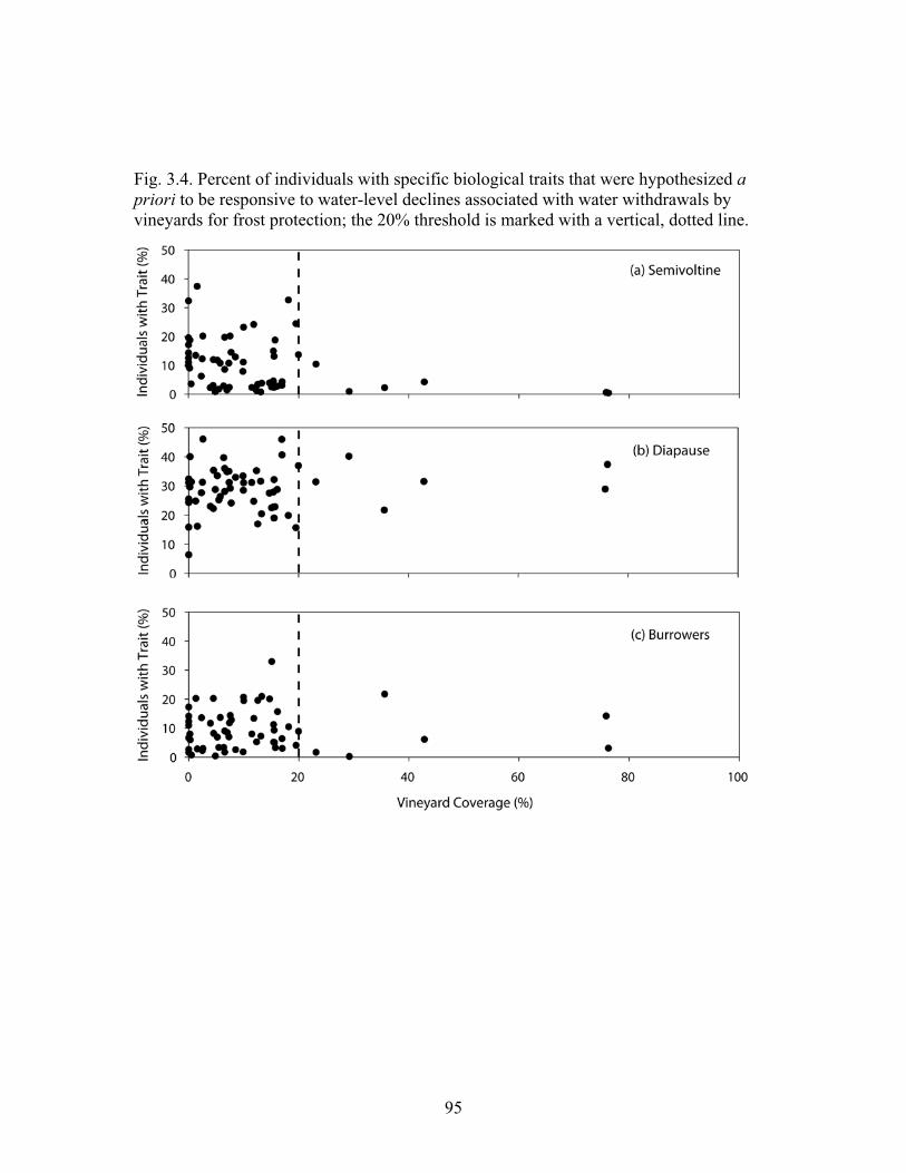
Fig. 3.4. Percent of individuals with specific biological traits that were hypothesized apriori to be responsive to water-level declines associated with water withdrawals by vineyards for frost protection; the 20% threshold is marked with a vertical, dotted line.

95

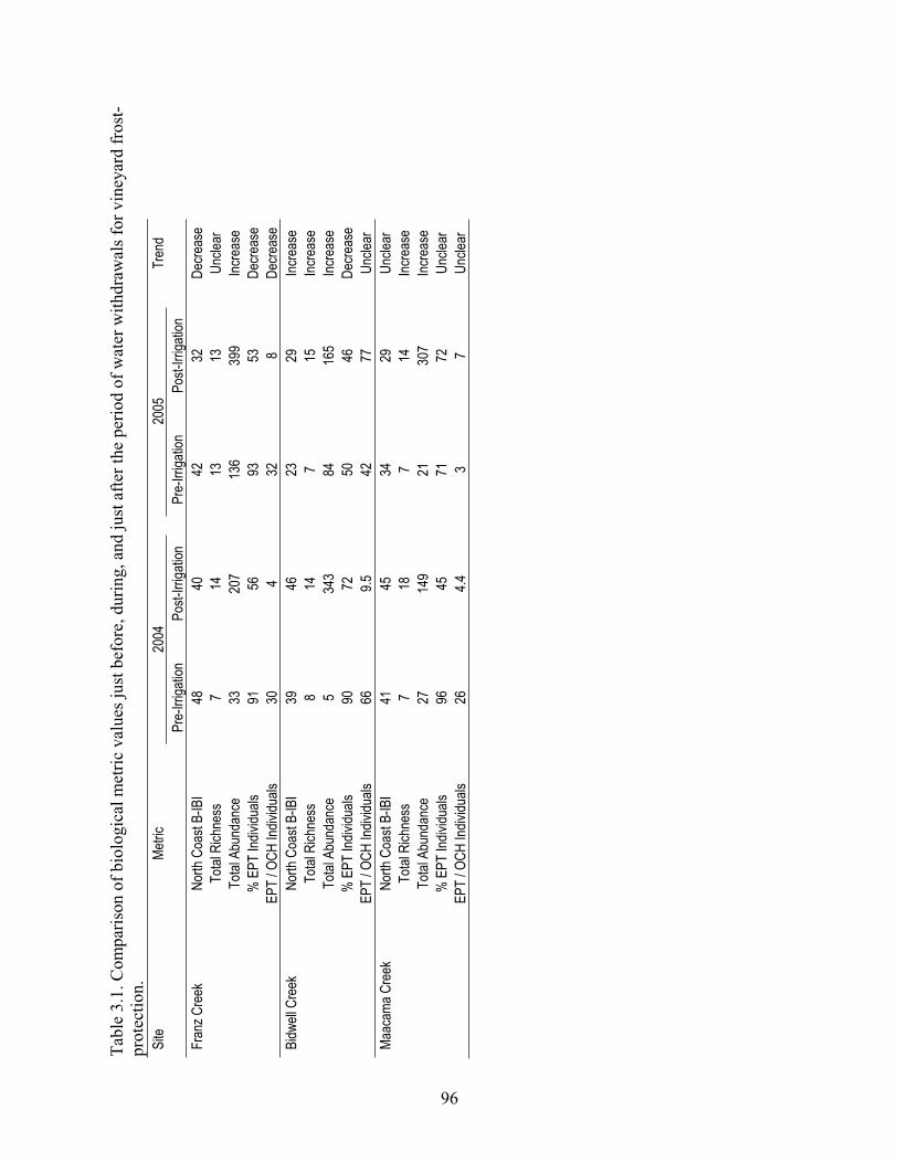
Tabl

e 3.

1. C

ompa

rison

of b

iolo

gica

l met

ric v

alue

s jus

t bef

ore,

dur

ing,

and

just

afte

r the

per

iod

of w

ater

with

draw

als f

or v

iney

ard

fros

t-pr

otec

tion.

Site

Me

tric

20

04

20

05

Tr

end

Pre-

Irriga

tion

Po

st-Irr

igatio

n

Pre-

Irriga

tion

Po

st-Irr

igatio

n

Fr

anz C

reek

North

Coa

st B-

IBI

48

40

42

32

De

creas

e

To

tal R

ichne

ss

7

14

13

13

Uncle

ar

Total

Abu

ndan

ce

33

207

13

6

399

Inc

reas

e

%

EPT

Indiv

iduals

91

56

93

53

Decre

ase

EPT

/ OCH

Indiv

iduals

30

4

32

8

Decre

ase

Bidw

ell C

reek

North

Coa

st B-

IBI

39

46

23

29

Inc

reas

e

To

tal R

ichne

ss

8

14

7

15

Inc

reas

e

To

tal A

bund

ance

5

343

84

165

Inc

reas

e

%

EPT

Indiv

iduals

90

72

50

46

Decre

ase

EPT

/ OCH

Indiv

iduals

66

9.5

42

77

Uncle

ar

Maac

ama C

reek

North

Coa

st B-

IBI

41

45

34

29

Un

clear

To

tal R

ichne

ss

7

18

7

14

Inc

reas

e

To

tal A

bund

ance

27

14

9

21

30

7

Incre

ase

% E

PT In

dividu

als

96

45

71

72

Un

clear

EP

T / O

CH In

dividu

als

26

4.4

3

7

Un

clear

96

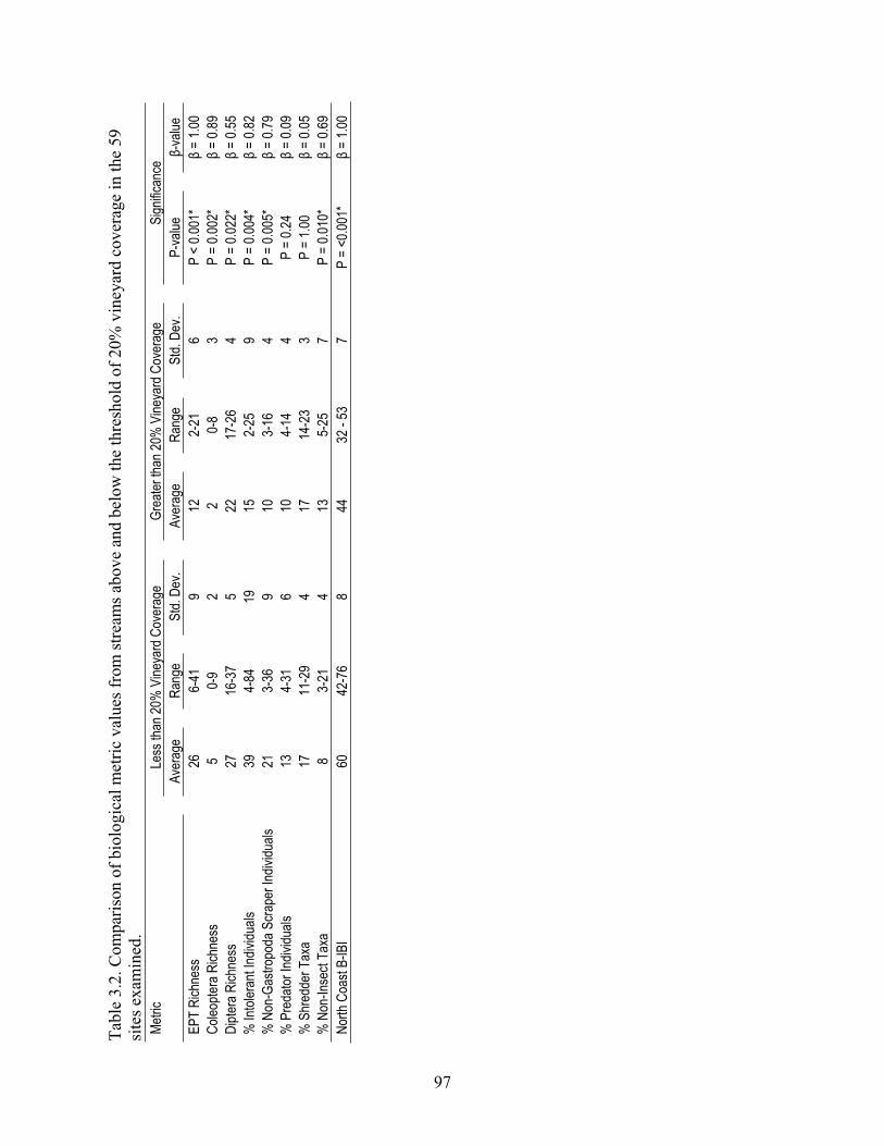
Tabl

e 3.

2. C

ompa

rison

of b

iolo

gica

l met

ric v

alue

s fro

m st

ream

s abo

ve a

nd b

elow

the

thre

shol

d of

20%

vin

eyar

d co

vera

ge in

the

59si

tes e

xam

ined

. Me

tric

Le

ss th

an 20

% V

ineya

rd C

over

age

Gr

eater

than

20%

Vine

yard

Cov

erag

e

Sign

ifican

ce

Aver

age

Ra

nge

St

d. De

v.

Aver

age

Ra

nge

St

d. De

v.

P-va

lue

-va

lueEP

T Ri

chne

ss

26

6-41

9

12

2-

21

6

P

< 0.0

01*

=

1.00

Co

leopte

ra R

ichne

ss

5

0-

9

2

2

0-8

3

P

= 0.0

02*

=

0.89

Di

ptera

Rich

ness

27

16

-37

5

22

17-2

6

4

P =

0.022

*

= 0.

55

% In

toler

ant In

dividu

als

39

4-84

19

15

2-25

9

P =

0.004

*

= 0.

82

% N

on-G

astro

poda

Scra

per I

ndivi

duals

21

3-

36

9

10

3-16

4

P =

0.005

*

= 0.

79

% P

reda

tor In

dividu

als

13

4-31

6

10

4-

14

4

P

= 0.2

4

= 0.

09

% S

hred

der T

axa

17

11-2

9

4

17

14

-23

3

P

= 1.0

0

= 0.

05

% N

on-In

sect

Taxa

8

3-21

4

13

5-

25

7

P

= 0.0

10*

=

0.69

No

rth C

oast

B-IB

I

60

42

-76

8

44

32 -

53

7

P

= <0

.001*

= 1.

00

97

CHAPTER 4

Physical-habitat restoration in the Lagunitas Creek Watershed, Marin County, California: Evaluating the effects of large wood on pool formation in streams

98

Physical-habitat restoration in the Lagunitas Creek Watershed, Marin County, California: Evaluating the effects of large wood on pool formation in streams

Abstract

Physical-habitat complexity is essential for supporting aquatic fauna. Large wood, live and dead, is especially important for producing high-quality physical-habitat in forested streams. I examined five, 300-m stream reaches in a watershed in Northern California to determine: 1) the amount of large wood in the bankfull channel; 2) the amount of large wood available for recruitment from the riparian zones; 3) the influence of large wood on the size and distribution of pools; 4) whether streams with large-wood additions had a greater diversity of large wood and pool habitat than streams without; and 5) how large wood levels in streams in this watershed compare with other streams in western North America. I found that the amount of large wood in the bankfull channel and the amount available for recruitment varied highly among streams. Large wood in the bankfull channel, particularly wood pieces with root-wads or those that were part of clusters, had a very strong influence on pool formation. Of the large wood pieces that were a primary pool-forming factor, 76% were part of a cluster and 21% had a root-wad. Stream reaches with large-wood additions in the form of engineered wood structures had lower values of channel widths per pool than those without large-wood additions (1.3-2.0 vs. 2.6-5.0). This increase in pool frequency would have a predictably favorable benefit for over-winter survival of juvenile coho salmon (Oncorhynchus kisutch), which was one of the primary goals of the large-wood additions. The streams in this study generally had lower volumes of large wood and higher values of channel widths per pool than streams of comparable size in the Western United States.

Key words: physical habitat, restoration, large woody debris, pool formation, streams

99

Introduction

Rivers and streams can be classified into different hierarchies or types based on their characteristic geomorphic features and events and the complexity of physical habitat will be different for different river or stream types (Frissel et al. 1986). For example, large rivers in the Midwest might have very different definitions of physical-habitat complexity than forested streams in the Pacific Northwest. Complexity of physical habitat in a forested stream reach is characterized by a range of abiotic or physical conditions, including pools (Quinn and Peterson 1996), riffles (Pearsons et al. 1992), wood in the stream channel (O'Connor 1991), undercut banks (Horan et al. 2000), different levels of shading as a result of differences in canopy coverage (Eriksson et al. 2006), and temperature differences as a result of both shading and groundwater inflows (Quinn and Peterson 1996, Poole and Berman 2001). In contrast, low physical-habitat complexity along such a stream reach would have low diversity of these conditions.

Physical-habitat complexity in forested streams is important for aquatic organisms because it results in a variety of ecological niches, which provide the foundation to support a high level of biodiversity (Ward and Tockner 2001, Johnson et al. 2003). Biodiversity can be defined as the number and variety of taxa in a region (Bengtsson 1998). Because individual taxa are specialized or adapted to take advantage of a specific set of physical conditions, the presence of highly diverse physical-habitat conditions can thus support a higher number of distinct taxa (Collier 2008, Péru and Dolédec 2010). Wood in forested streams increases physical-habitat complexity by creating niches for aquatic organisms that live and feed directly on wood itself (O'Connor 1991) and for those that live in the pools that form as a result of the wood (Bonada et al. 2009). Wood is associated with pool formation because it creates conditions during high flows that can promote localized scour of the streambed (Borg et al. 2007, Mao et al. 2008). The size and orientation of wood in streams can affect the size of the pools that form during these high flow events (Wohl et al. 2010). Whether the wood is living or dead is also important because it affects the length of time that the wood stays in place and thus the length of time that the associated pools persist (Opperman and Merenlender 2007, Opperman et al. 2008). The amount of large wood in many forested streams of the western United States has been reduced as a result of both lower recruitment because of logging in riparian areas and prescribed removal to address problems such as scour near stream-side roads and collection of wood near bridge abutments, which can cause erosion and thereby reduce the structural integrity of the roads or bridges (Mellina and Hinch 2009, Wondzell et al. 2009). In addition, there was a misperception for many years that large wood in streams was not favorable, partly because it was not aesthetically pleasing (Opperman et al. 2008). Although large-wood removal programs, often called river or stream cleanup projects, have officially ceased in most areas, large wood continues to be removed from streams by some management personnel out of habit, and the effects of large-wood removal can persist for years after the programs end because it can take a long time for new large-wood recruitment to occur from the surrounding riparian area and from the watershed upstream (Martin and Benda 2001, May and Gresswell 2003). The amount of large wood in forested streams and the diversity of pool habitat are highly influenced by local conditions, such as the type of riparian forest and the streambed substrate (Buffington et al. 2002). Many studies of large wood in forested streams in the western United

100

States have been conducted in the Pacific Northwest where the climate is temperate (Montgomery et al. 1995, Buffington et al. 2002, May and Gresswell 2003). In contrast, a smaller number of studies have been conducted in the north-coast region of California, where the climate is mediterranean (Opperman and Merenlender 2007, Opperman et al. 2008). Differences between these regions, in terms of the amount of large wood and pools, remain largely unexplored. Physical-habitat restoration is being undertaken in streams in both these regions, motivated by the desire to increase fish populations (Gerhard and Reich 2000, Gurnell et al. 2002, Roni et al. 2002, Kail et al. 2007).

This study was conducted in a watershed in northern California, where a physical-habitat restoration project was being carried out to improve rearing habitat for the coho salmon (Oncorhynchus kisutch) population. The objectives of this study were to determine: 1) the amount of large wood in the channels; 2) the amount available for recruitment from the riparian zones; 3) the influence of large wood on the size and distribution of pools; 4) whether streams with the addition of engineered, large-wood structures had a greater diversity pool habitat than streams without; and 5) how streams in this watershed compare with streams elsewhere. These objectives have implications for physical-habitat restoration in streams in the Mediterranean-climate region of Northern California, and potentially in streams elsewhere where engineered wood structures are being considered for installation.

Methods

Site Description The study sites included five 300-m reaches along three streams in the Lagunitas Creek watershed in Marin County, California (Table 4.1). Three sites were located on the mainstem of Lagunitas Creek (LAG1, LAG2, and LAG3) and two were located on separate tributaries to the mainstem, San Geronimo Creek (SAN) and Devil's Gulch (DEV) (Fig. 4.1). The study was conducted in the spring and summer (April – August) of 2009 and 2010. The sites were selected for study because they had either already undergone or were being considered as potential sites for physical-habitat restoration in the form of engineered, large-wood structures. These structures are intended to promote pool formation, to slow downstream migration of sediment, and to increase high-flow refuge and improve summer rearing habitat for salmonids (O'Connor and Rosser 2006). The Lagunitas Creek watershed was logged extensively in the 1800s, dammed in the early 1800s through the 1950s, and regularly subjected to large wood removal from stream channels during the 1970s and 1980s; all of these factors have contributed to a reduced amount of large wood present in the stream channels relative to natural levels (O'Connor and Rosser 2006). The large wood for the engineered structures is primarily coast redwood (Sequoia sempervirens), which was obtained from reservoirs upstream in the watershed, such as Kent Lake, where it had collected as debris behind dams. Three of the sites selected for study (LAG1, LAG2, and DEV) were located in Samuel P. Taylor State Park with riparian zones composed predominately of coast redwood forest (S.sempervirens), whereas the other two sites (SAN and LAG3) were located outside of the State Park in riparian zones composed of California bay laurel (Umbellularia californica), willow (Salix spp.), and alder (Alnus spp.). Engineered large-wood structures had been installed at LAG1 and LAG2 prior to this study (Table 3.1).

101

The physical-habitat restoration projects in this watershed were largely driven by a local effort to protect coho salmon populations. Although coho salmon populations across the state of California have declined since the start of the last century (Brown et al. 1994), the coho population in the Lagunitas Creek watershed remains one of the largest and most stable in California (Ketcham et al. 2004).

Large Wood Large wood was defined as any portion of wood, live or dead, with a diameter of at least 10 cm, following other studies (Dolloff and Warren 2003, Lassettre 2003, Opperman and Merenlender 2007). Dead large wood was classified as large woody debris (LWD), whereas living large wood was classified as large live wood (LLW). Many studies have established the importance of LWD on pool formation in streams, including studies conducted in the mediterranean-climate region of California (Lassettre 2003) and studies conducted in the Pacific Northwest of the United States (Montgomery et al. 1995), and the importance of LLW on pool formation in streams is increasingly being recognized (Opperman and Merenlender 2007). The large-wood inventory was conducted in both the bankfull channel and the approximate 10-year floodplain outside the bankfull channel. The typical recurrence interval of the discharge that fills the bankfull channel and mobilizes bed material is approximately 1.5 years (Dunne and Leopold 1978). The dimensions of the bankfull channel were approximated visually by assessing vegetation, recent high-water marks, and the elevation of freshly deposited gravel bars. The width of the 10-year floodplain was approximated visually by searching for evidence of flood terraces containing a substantial portion of vegetation within the 10-year seral stage.

A pool-forming factor was defined as a physical structure in the bankfull channel or 10-year floodplain that participated in pool formation. Pool-forming factors were determined by visual assessment. The pool-forming factors considered included boulder (BO), bedrock (BR), alluvial bar-riffle (A), step (S), or large wood (W). Structures in the 10-year floodplain were considered pool-forming factors only if they provided anchorage or support for wood in the bankfull channel that was associated with pool formation.

For each piece of large wood that was encountered, I determined: 1) the location along the longitudinal profile; 2) whether it was dead (LWD) or living (LLW); 3) the length of the piece contained within the 10-year floodplain; 4) the average diameter; 5) whether a root-wad was present; 6) whether it was coniferous or hardwood; 7) whether it was pool-forming factor; 8) whether it was part of a cluster (i.e., greater than three pieces in contact with each other); 9) whether it was standing upright, and 10) whether it was added as part of an engineered, large-wood structure.

Size and Distribution of Pools A pool was defined as any portion of the stream with a minimum water depth of 0.5 m. Minimum water-depth criteria are commonly used for defining pools in both geomorphic (Montgomery et al. 1995) and biological (Calhoun et al. 2003) studies. For each pool in this study, I determined the location along the longitudinal profile, the length, the average width, the maximum depth, and the primary pool-forming factor. The area of each pool was calculated using the measured length and width.

102

Data comparisons The sites with engineered, large-wood structures were compared to those without on a site-specific basis. The comparisons included the following variables; 1) total number of pieces of LWD per m2 in the bankfull channel, 2) total volume (m3) of LWD in the bankfull channel, 3) total number of pools, 4) total area of pools, 5) deepest pool, and 6) channel widths per pool.The sites with and without engineered, large-wood structures could not be treated as replicates for statistical comparisons because the reaches examined differed in many uncontrolled variables such as riparian vegetation type and substrate type and a much larger number of sites would have been necessary to examine in order to parse out the influence of these variables. The condition of the sites prior to the installation of the engineered, large-wood structures is unknown.

The information from the sites was compared with similar data from other sites in North America, and inferences were made for over-winter survival of coho salmon based on previously observed relationships in a stream in Washington. For example, the volume of LWD per m2 in the bankfull channel was compared with other sites in the Mediteranean climate region of California and elsewhere in North America (Lassettre 2003). The measured number of pieces of LWD per m2 in the bankfull channel and the measured channel widths per pool were compared to similar information in Montgomery et al. (1995) for 46 sites in the states of Washington and Alaska. Lastly, a prediction of the over-winter survival (%) of juvenile coho salmon was extrapolated from a relationship between the over-winter survival (%) and channel widths per pool that was determined by Quinn and Peterson (1996) for a small stream in Washington.

Results

Large Wood Bankfull Channels

I measured 556 total pieces of large wood in the bankfull channel. The number of pieces of LWD per reach ranged from 20 to 151 (mean = 66, SD = 53) and the number of pieces of LLW ranged from 7 to 159 (mean = 45, SD = 65). LWD comprised 60 % of the total number of pieces of large wood. The LWD was composed of 15 % hardwood (85 % coniferous), whereas the LLW was composed of 99 % hardwood (1 % coniferous). 42% of LWD pieces acted as a pool-forming factor, compared to 27% of LLW pieces. Of the LWD pieces that functioned as pool-forming factors, 21 % had a root-wad, 76 % were part of a cluster, 4 % were standing upright, and 12 % were associated with the engineered, large wood structures. Of the LLW pieces, 34 % had a root-wad, 41 % were part of a cluster, 66 % were standing upright, and 0 % were associated with the engineered, large wood structures. Per area of bankfull channel, the average amount of LWD that was available within the reaches was roughly twice the average amount of LLW (Table 4.2).

10-year Floodplains outside of the Bankfull Channels I measured 529 total pieces of large wood in the 10-year floodplains outside of the bankfull channel. The number of pieces of LWD per reach ranged from 16 to 53 (mean = 27, SD = 15) and the number of pieces of LLW ranged from 8 to 298 (mean = 88, SD = 121). LWD comprised 26 % of the total number of pieces of large wood and was composed of 94 % hardwood (6 % coniferous), whereas the LLW was composed of 99 % hardwood (1 % coniferous). 17% of LWD pieces acted as a pool-forming factor, compared to 5% of LLW pieces. Of the LWD pieces that functioned as pool-forming factors, 0 % had a root-wad, 96 %

103

were part of a cluster, 0 % were standing upright, and 0 % were associated with the engineered, large wood structures. Of the LLW pieces, 44 % had a root-wad, 88 % were part of a cluster, 94 % were standing upright, and 0 % were associated with the engineered, large wood structures.Per area of bankfull channel, the average amount of LWD that was available within the reaches was roughly half the average amount of LLW (Table 4.2).

Size and Distribution of Pools I measured a total of 51 pools among the study sites (Table 4.3). The average number of pools was 10 (SD = 4), the average total area of pools was 244 m2 (SD = 191), the average depth of the deepest pool was 1.3 m (SD = 0.5), the average distance between pools was 36 m (SD = 22), the average number of channel widths per pools was 3 (SD = 2), and the primary pool-forming factors were wood and bedrock (Table 4.3). Wood was identified as the primary pool-forming factor in 36 out of the 51 pools measured (71%). Bedrock was the second most important primary pool-forming factor, accounting for roughly one quarter of the pools.

Comparison of sites with and without large-wood additions The total number of pieces of LWD per m2 in the bankfull channel at the sites with engineered, large wood structures was within the same range of those sites without structures, i.e., 0.011 – 0.018 pieces per m2 (Table 4.1). In contrast, the total volume of LWD was higher at the sites with structures than those sites without structures (Table 4.1). The total number of pools was relatively high at one of the sites with structures, but not at the other site with structures (Table 4.2). The depth of the deepest pool at the sites with structures was within the same range of those sites without structures, and so was the average distance between pools (Table 4.2). The pool frequency was higher at the two sites with structures than at the sites without structures (Table 4.2).

Comparison of sites with streams in other regions The total volume of LWD / m2 observed in the bankfull channel at each of the sites, which ranged from 0.014 – 0.017 m3/m2 (Table 4.2), is very close to the total volume that was observed in Lower East Branch Soquel Creek (0.005 m3/m2) (Lassettre 2003), another disturbed coast redwood stream in the Mediterranean climate region of Northern California, and is notably lower than the amounts of LWD found in undisturbed coast redwood streams in Redwood National Park (Keller and MacDonald 1983) and elsewhere in North America (Lassettre 2003). In comparison to streams in Washington and Alaska of comparable size, i.e., those with bankfull widths <15 m, the sites I examined in coastal California all had relatively low large- woody-debris coverage per area of bankfull channel (Fig. 4.2). However, the sites with large-wood additions had a lower value of channel widths per pool, which was closer to the values reported for the majority of the streams in Washington and Alaska (Fig. 4.2). Based on the channel widths per pool measured in this study, the sites with large-wood additions are predicted to have a higher percentage of over-winter survival of juvenile coho salmon than the sites without large-wood additions (Fig. 4.3). The total volume of LWD / m2 observed at each of the sites (Table 2) was very close to the total volume that was observed in Lower East Branch Soquel Creek (0.005 m3/m2) (Lassettre 2003), another disturbed coast redwood stream in the Mediterranean climate region of Northern California, and is notably lower than the amounts of LWD found in undisturbed coast redwood streams in Redwood National Park and elsewhere in North America (Lassettre 2003).

104

Discussion

The high variability in the amount of both LWD and LLW among the sites examined (Table 4.2) is related to natural physical-habitat differences, such as riparian-vegetation type and substrate type. For example, LAG1, LAG2, and DEV were located in coast redwood forests, whereas the other sites were located in hardwood forests. LAG3 contained dense alder thickets, which account for the relatively high number of pieces of large wood measured in this reach (Table 4.2). LAG2 and DEV contained a larger portion of bedrock substrate than the other sites, and thus bedrock was relatively more important as a pool-forming factor at these sites. The relatively low number of pieces of LWD per m2 available for recruitment from the 10-year floodplain in the two sites with large-wood structures installed provides evidence that the addition of LWD pieces to these sites was appropriate because less was available for natural recruitment. Human activities have certainly reduced the amount of LWD reaching the lower reaches of the Lagunitas Creek watershed. However, the amount of large wood that was impounded behind dams and selectively removed from the streams over the past decades is unknown. This makes it impossible to ascertain exactly the amount of large wood that would otherwise have been present in the bankfull channel if dams had not been added to Lagunitas Creek. Nonethess, because the average biomass of LWD in the bankfull channel of the three coast redwood sites (7.1 kg/m2 assuming a standard wood density of 450 kg/m3) was dramatically less than the average biomass reported by Bilby and Bisson (1998) for typical Northern California redwood forest (74.2 kg/m2), it is highly likely that these reaches are wood starved. The loss of LWD recruitment from the upper reaches of the watershed by Peters Dam, which was built in 1954 to form Kent Lake, has surely reduced the amount of LWD passing through the two reaches in this study that had undergone additions of engineered, large wood structures (LAG1 and LAG2). Large wood is an important pool-forming factor in streams (Bilby and Ward 1991, Montgomery et al. 1995, Beechie and Sibley 1997). In sites throughout Washington and Alaska, LWD in bankfull channels was associated with pool formation in less than 40% of cases (Montgomery et al. 1995). In sites in this study, LWD was associated with pool formation in slightly greater than 42% of cases. The sites in Washington and Alaska were in high-gradient (slope 2%), mountain drainage basins (Montgomery et al. 1995) and the sites in this study were in lower-gradient (slope 1%), coastal drainage basins. This could explain the relatively high effectiveness of LWD in pool formation in the study sites. However, a 1% slope is still steep relative to many streams elsewhere. In high-gradient basins, large boulders tend to override LWD as dominant pool-forming factors (Beechie and Sibley 1997). Root-wads at the end of pieces of large wood promote pool formation in streams (Opperman 2007, Warren and Bernhardt 2007), which was supported by data from this study. Whether the large wood was part of a cluster or jam was also found to be important, which has been confirmed by others (Rosenfeld and Huato 2003). In agreement with Opperman (2007) and Opperman et al. (2008), LLW featured prominently in the large-wood clusters measured. The engineered, large-wood structures had a notable effect on pool formation. For example, LWD in engineered, large wood structures made up 12% of the total LWD pieces that were pool-forming factors in the bankfull channel. There was also modest evidence from this study that the engineered, large-wood structures lowered the channel widths per pool, which is equivalent to an increase in pool frequency (Table 3). Other studies have shown that pool

105

frequency is often related to LWD levels (Montgomery et al. 1995, Beechie and Sibly 1997, Lassettre 2003). Lassettre (2003) observed 75-80% of pools to be associated with LWD in two streams in the Mediterranean-climate region of California. In this study, for comparison, LWD was observed to be a primary pool-forming factor in 71% of pools, and this percentage would be higher if secondary pool-forming factors were included. Post-project monitoring and assessment by the Marin Municipal Water District has shown that pools have formed and increased in size in the years following the large-wood addition (E. Ettlinger, personal communication). The number of trees per m2 and the biomass of trees per m2 in Mediterranean-climate regions is typically less than it is in temperate-climate regions because of rainfall and temperature patterns (Scarascia-Mugnozza et al. 2000). This generalization could explain why the sites in this study contained less LWD per m2 than most of the sites of comparable size in Washington and Alaska (Fig. 4.2). However, there were streams in Washington and Alaska in the same range of LWD per m2 as measured at the study sites, which suggests that knowledge acquired from studies conducted on streams in other regions, such as parts of the Pacific Northwest, should be transferrable to some extent to studies and watershed-management projects conducted on streams in the Mediterranean-climate region of California and potentially in Mediterranean regions elsewhere. Pool frequency in steeper, step-pool channels, where large boulders are the dominant pool-forming mechanism, tend to be lower than in low-gradient, pool-riffle channels such as the study sites, and to be independent of LWD (Montgomery et al 1995). This difference explains the tendency of the channel widths per pool at the sites in this study to be higher on average than most of the sites of comparable size in Washington and Alaska (Fig. 4.2). The lower channel widths per pool, i.e., higher pool frequencies, at the two sites with engineered, large wood structures were closer to most of the values of channel widths per pool observed for streams in Washington and Alaska. The lower channel widths per pool values observed in the sites with the engineered, large-wood structures (Fig. 4.3) combined with the regression relationships from Quinn and Peterson (1996) suggests the possibility of potentially increased over-winter survival of juvenile coho salmon in the Lagunitas watershed. Higher over-winter survival was one of the primary goals of the physical-habitat restoration projects. The engineered, large-wood structures, and their associated pools, could increase over-winter survival by providing refuge during winter high flows, which typically occur between the months of December and April in this region of California (Gasith and Resh 1999). In addition, the lower distance between pools could make it easier for fish that are swept downstream by high flows to return upstream because they could rest in each of the pools along the way and would have a shorter distance over which they would need to expend energy in order to reach the next pool upstream. In conclusion, the characteristics of habitat complexity are highly variable among stream reaches, between regions, and within the same watershed. Physical-habitat in streams is influenced by local environmental constraints as well as past human activities. In this study, I observed evidence that large wood had a strong effect on pool formation, with roots wads and clusters being especially important. Engineered, large wood structures had the effect of potentially increasing pool frequency. Although the information contained in this study is site-specific, there is modest evidence that similar approaches may be useful in other regions.

106

Acknowledgements

I thank the US Department of Agriculture Forest Service (USFS) under Cost Share Agreement #03-CR-11052007–042 and the Edward A. Colman Fellowship in Watershed Management from the Department of Environmental Science, Policy, and Management at the University of California, Berkeley, for support. I also thank M. Cover for assistance with this study design and assistance in the field, J. Ball for assistance in the field, and J. McBride for comments on this chapter.

Literature Cited

Beechie, T.J., and Sibley, T.H. 1997. Relationships between channel characteristics, woody debris, and fish habitat in Northwestern Washington Streams. Transactions of the American Fisheries Society 126: 217-229.

Bengtsson, J. 1998. Which species? What kind of diversity? Which ecosystem function? Some problems in studies of relations between biodiversity and ecosystem function. Applied Soil Ecology 10: 191-199.

Bilby, R.E., and Bisson, P.A. 1998. Function and distribution of large woody debris. p. 324-346. In: R.J. Naiman and R.E. Bilby (eds.) River ecology and management: lessons from the Pacific coastal ecoregion. Springer-Verlag, New York, NY.

Bilby, R.E., and Ward, J.W. 1991. Characteristics and function of large woody debris in streams draining old-growth, clear-cut, and second-growth forests in Southwestern Washington. Canadian Journal of Fisheries and Aquatic Sciences 48: 2499-2508.

Bonada N., Rieradevall M., Prat N., Resh, V.H. 2009. Benthic macroinvertebrate assemblages and macrohabitat connectivity in Mediterranean-climate streams of Northern California. Journal of the North American Benthological Society 25: 32–43.

Borg, D., Rutherford, I., and Stewardson, M. 2007. The geomorphic and ecological effectiveness of habitat rehabilitation works: continuous measurement of scour and fill around large logs in sand-bed streams. Geomorphology 89: 205-216.

Brown, L. R., Moyle, P. B., and Yoshiyama, R. M. 1994. Historical decline and current status of coho salmon in California. North American Journal of Fisheries Management 14: 237-261.

Buffington, J.M., Lisle, T.E., Woodsmith, R.D., and Hilton, S. 2002. Controls on the size and occurrence of pools in coarse-grained forest rivers. River Research and Applications 18: 507-531.

Calhoun, A.J.K., Walls, T.E., Stockwell, S.S. and McCollough, M. 2003. Evaluating vernal pools as a basis for conservation strategies: a Maine case study. Wetlands 23: 70-81.

107

Collier, K.J. 2008. Temporal patterns in the stability, persistence and condition of stream macroinvertebrate communities: relationships with catchment land-use and regional climate. Freshwater Biology 53: 603-616.

Eriksson B.K., Rubach, A., and Hillebrand, H. 2006. Biotic habitat complexity controls species diversity and nutrient effects on net biomass production. Ecology 87: 246-254.

Gerhard, M. and Reich, M. 2000. Restoration of streams with large wood: effects of accumulated and built-in wood on channel morphology, habitat diversity and aquatic fauna. International Review of Hydrobiology 85: 123-137.

Gurnell, A.M., Piégay, H., Swanson, F.J., and Gregory S.V. 2002. Large wood and fluvial processes. Freshwater Biology 47: 601-619.

Horan, D.L., Kershner, J.L., Hawkins, C.P. and Crowl, T.A. 2000. Effects of habitat area and complexity on colorado river cutthroat trout density in Uinta Mountain streams. Transactions of the American Fisheries Society 129: 1548-8659.

Johnson, M.P, Frsot, N.J., Mosley, M.W.J., Roberts, M.F., and Hawkins, S.J. 2003. The area-independent effects of habitat complexity on biodiversity vary between regions. Ecology Letters 5: 126-132.

Kail, J., Hering, D., Muhar S., Gerhard, M., and Preis, S. 2007. The use of large wood in stream restoration: Experiences from 50 projects in Germany and Austria. Journal of Applied Ecology 44: 1145-1155.

Ketcham, B. J., Brown, G. G., and Wolff, O. G. 2004. index reach monitoring program summary - Olema Creek, Marin County, California: 1999-2003. PORE/NR/WR/04-04.

Lassettre, N.S., 2003. Process based management of large woody debris at the basin scale.Dissertation. University of California, Berkeley. 130 pp.

Mao, L., Andreoli, A., Comiti, F., and Lenzi, M.A. 2008. Geomorphic effects of large wood jams on a sub-antarctic mountain stream. River Research and Applications 24: 249-266.

May, C., and Gresswell, R.W. 2003. Large wood recruitment and redistribution in headwater streams in the southern Oregon Coast Range, U.S.A. Canadian Journal of Forest Research 33: 1352-1362.

Mellina, E., and Hinch, S.G. 2009. Influences of riparian logging and in-stream large wood removal on pool habitat and salmonid density and biomass: A meta-analysis. Canadian Journal of Forest Research 39: 1280-1301.

Montgomery, D. R., Buffington, J. M., Smith, R. D., Schmidt, K. M. and Pess, G., 1995. Pool spacing in forest channels. Water Resources Research 31: 1097-1105.

108

O'Connor, N.A. 1991. The effects of habitat complexity on the macroinvertebrates colonising wood substrates in a lowland stream. Oecologia 85: 504-512.

O'Connor, M., and Rosser, B. 2006. Lagunitas Creek fine sediment investigation. Technical Report prepared for the Marin Municipal Water District. Corte Madera, California. March 8, 2006.

Opperman, J. J., and Merenlender, A. M. 2007. Living trees provide stable large wood in streams. Earth Surface Processes 32: 1229-1238.

Opperman, J.J., Meleason, M., Francis, R.A., Davies-Colley, R. 2008. 'Livewood': geomorphic and ecological functions of living trees in channels. Bioscience 58: 1069-1078.

Pearsons, P.N., Hiram, W.L., and Lamberti, G.A. 1992. Influence of habitat complexity on resistance to flooding and resilience of stream fish assemblages. Transactions of the American Fisheries Society 121: 427-436.

Péru, N., Dolédec, S. 2010. From compositional to functional biodiversity metrics in bioassessment: a case study using stream macroinvertebrate communities. Ecological Indicators 10: 1025-1036.

Poole, G.C. and Berman, C.H. 2001. An ecological perspective on in-stream temperature: natural heat dynamics and mechanisms of human-caused thermal degradation. Environmental Management 27: 787-802.

Quinn T.P., and Peterson, N.P. 1996. The influence of habitat complexity and fish size on over-winter survival and growth of individually marked juvenile coho salmon (Oncorhynchus kisutch) in Big Beef Creek, Washington. Canadian Journal of Fisheries and Aquatic Sciences 53: 1555-1564.

Roni, P., Beechie, T.J., Bilby, R.E., Leonetti, F.E., Pollock, M.M., and Pess, G.R. 2002. A review of stream restoration techniques and a hierarchical strategy for prioritizing restoration in Pacific Northwest watersheds. North American Journal of Fisheries Management 22: 1-20.

Rosenfeld, J.S., and Huato, L. 2003. Relationship between large woody debris characteristics and pool formation in small coastal British Columbia streams. North American Journal of Fisheries Management 23: 928-938.

Scarascia-Mugnozza, G., Oswald, H., Piussi, P., and Radoglou, K. 2000. Forests of the Mediterranean region: gaps in knowledge and research needs. Forest Ecology and Management 132: 97-109.

Ward, J.V., and Tockner, K. 2001. Biodiversity: towards a unifying theme for river ecology. Freshwater Biology 46: 807-819.

109

Wohl, E., Cenderelli, D.A., Dwire, K.A., Ryan-Burkett, Young M.K., and Fausch, K.D. 2010. Large in-stream wood studies: a call for common metrics. Earth Surface Processes and Landforms 35: 618-625.

110

Table 4.1. Site information Site Location Latitude, Longitude Ave. Bankfull

Width (m) Number of Engineered,Large-Wood Structures

LAG1Lagunitas Creek upstream ofIrving Bridge

38°0'58.53"N,122°43'23.88"W 14.7 5

LAG2Lagunitas Creek upstreamof Confluence with Devil's Gulch

38°1'43.98"N,122°44'11.38"W 15.0 3

LAG3Lagunitas Creek along theTocoloma Reach

38° 3'6.25"N,122°45'36.76"W 11.5 0

SANSan Geronimo Creek by theWater Treatment Plant

38°0'45.09"N,122°39'8.30"W 6.2 0

DEVDevil's Gulch starting upstream of Sir Francis Drake Blvd.

38°1'46.27"N,122°44'9.44"W 5.1 0

111

Table 4.2. Number of pieces of large wood (LWD and LLW) per area of bankfull channel and total volume of large wood per area of bankfull channel, both within the bankfull channel and within the 10-year floodplain outside the bankfull channel, at each study site. * indicates sites with engineered, large-wood structures.

Location Reach LWD / m2 LLW / m2

Number of

PiecesTotal Volume

(m3)Number of

PiecesTotal Volume

(m3)Bankfull Channel LAG1* 0.012 0.017 0.003 <0.001 LAG2* 0.018 0.009 0.007 0.002 LAG3 0.044 0.004 0.046 0.003 SAN 0.011 0.005 0.008 0.004 DEV 0.017 0.005 0.005 0.001 Ave. (SD) 0.020 (0.014) 0.008 (0.005) 0.014 (0.018) 0.003 (0.001) 10-year Floodplain LAG1* 0.005 0.001 0.002 <0.001 Outside the LAG2* 0.006 0.001 0.020 0.001 Bankfull Channel LAG3 0.015 0.002 0.086 0.004 SAN 0.012 0.001 0.009 0.001 DEV 0.010 0.001 0.019 0.002 Ave. (SD) 0.010 (0.004) 0.001 (0.000) 0.027 (0.034) 0.002 (0.002)

112

Table 4.3. Characteristics of the size and distribution of the pools at the study sites; W = wood and BR = bedrock. * indicates sites with engineered, large-wood structures.

Site Numberof Pools

Total Area of Pools (m2)

Depth of Deepest Pool (m)

Ave. Distance Between Pools (m)

ChannelWidths/Pool

Primary Pool- Forming Factor

LAG1* 10 154 0.8 30 2.0 W (7/10) LAG2* 16 439 1.4 19 1.3 BR (8/16) & W(8/16) LAG3 10 446 1.6 30 2.6 W (10/10) SAN 11 165 1.9 27 4.4 W (10/11) DEV 4 15 0.9 75 5.0 BR (3/4)

Ave. (SD) 10 (4) 244 (191) 1.3 (0.5) 36 (22) 3.1 (1.6)

113

Fig. 4.1. Site map

114

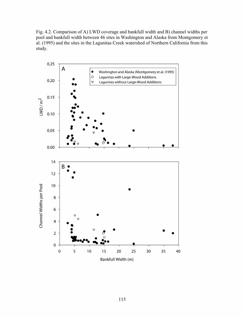
Fig. 4.2. Comparison of A) LWD coverage and bankfull width and B) channel widths per pool and bankfull width between 46 sites in Washington and Alaska from Montgomery et al. (1995) and the sites in the Lagunitas Creek watershed of Northern California from this study.

115

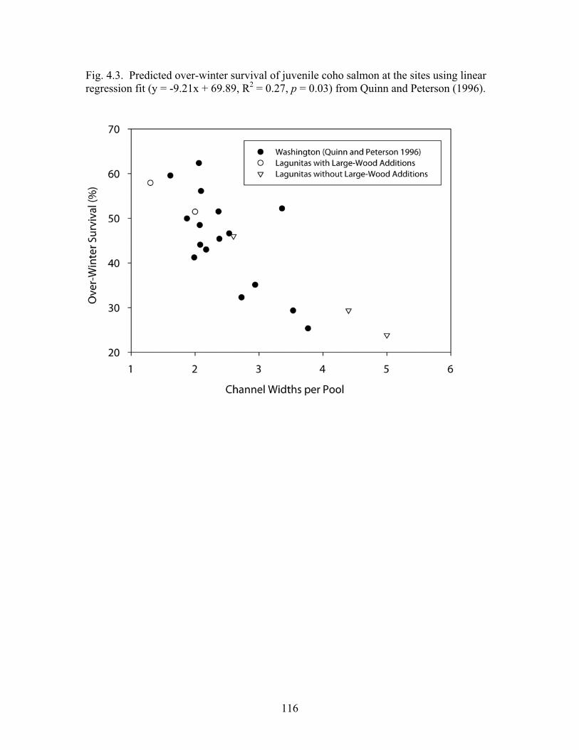
Fig. 4.3. Predicted over-winter survival of juvenile coho salmon at the sites using linear regression fit (y = -9.21x + 69.89, R2 = 0.27, p = 0.03) from Quinn and Peterson (1996).

116

CHAPTER 5

Physical-habitat restoration in the Lagunitas Creek Watershed, Marin County, California: Evaluating the effects of large wood on benthic macroinvertebrates

117

Physical-habitat restoration in the Lagunitas Creek Watershed, Marin County, California: Evaluating the effects of large wood on benthic macroinvertebrates

Abstract

Large-wood addition to streams is a common approach to restore physical-habitat complexity in streams where large wood has been removed by humans in the past or where dams installed in the watershed prevent recruitment of wood to the stream channel from upstream. The objective of this study was to determine: 1) the taxa occurring in pools created from engineered, large-wood structures used in restoration and the associated riffles; 2) taxa that are most likely to benefit from the creation of new pool-riffle sequences; and 3) long-term changes ( 9 years) in the benthic-macroinvertebrate community that have occurred temporally from in the restoration process. I observed % shredders to be significantly higher in created pools than in nearby riffles. The dominant shredders in pools were caddisflies, whereas the dominant shredders in riffles were stoneflies. I also observed statistically significant differences between pools and riffles using five benthic-macroinvertebrate community metrics. From early to late in restoration, significantly lower percentages of scrapers and shredders were observed in riffles, there were significant changes observed in the four of the five community metrics examined, and riffles were supporting more taxa with strong preferences for riffle habitat.Increases in relative abundances of Ephemeroptera, Plecoptera, and Trichoptera (EPT) taxa indicate water quality improvement. Coho salmon (Oncorhynchus kisutch) should benefit from the increase in EPT taxa observed, which was one of the primary stated goals of the restoration.

Key words: habitat restoration, large wood, benthic macroinvertebrates, biological monitoring

118

Introduction

Physical-habitat complexity or heterogeneity in streams is important for benthic macroinvertebrates because they can inhabit the variety of niches that a highly complex physical-habitat provides (O'Connor 1991, Bis et al. 2000). For example, some benthic-macroinvertebrate taxa are specialized to feed on wood (O'Connor 1991), whereas others are specialized to withstand strong water current (Lancaster et al. 1990). The diversity of pool and riffle habitat is an especially relevant aspect of physical-habitat complexity for benthic macrointertebrates in small streams (Brussock and Brown 1991). Taxa that are found more often in pools than in riffles are often adapted to the lower oxygen levels (Connolly et al. 2004, Jacobson 2008), slower moving water (Dolédec et al. 2007), and/or greater water depth (Bonada et al 2006). Other important aspects of physical habitat include amounts and types of large wood in the stream channel (Hilderbrand et al. 1997), undercut banks (Barbour et al. 1996, Meyers and Resh 2000), water temperature (Bonada et al 2006), and shading from vegetation (Li and Dudgeon 2008). Stream reaches with an abundance of pool-riffle sequences can support a higher level of biodiversity, and are thus important for conservation efforts (Schwartz and Herricks 2007). Pools and riffles influence not only benthic macroinvertebrates (Bonada et al. 2006), but also the fishes and birds that prey on them (Schwartz and Herricks 2007), the organisms at higher trophic levels that prey on the fishes and birds, and the composition of decomposer communities that recycle nutrients to the stream ecosystem (Rincón and Santelloco 2009). Many taxa in the orders Ephemeroptera, Plecoptera, and Trichoptera, which are more commonly found in riffles than in pools, are an important component in the diet of fish (Wooster and Sih 1995). Many taxa in the order Coleoptera, which are more commonly found in pools than in riffles (Forno et al. 1983), are an important component in the diets of some birds and mammals (Pavey et al. 2009). The specific combination of taxa that occupy stream reaches in a particular watershed are often unique to that location, and this combination is influenced by a large range of factors including physical habitat, past environmental conditions, such as floods, droughts, and human disturbance, the order of arrival of colonizing species, and the introduction of non-native or invasive species (Oertli et al. 2008, Brown et al. 2009).Background knowledge of the benthic-macroinvertebrate communities that occupy a stream reach can be useful to consider in physical-habitat restoration in streams because the composition of these communities is likely to change in response to the restoration practices followed and these changes can be used to evaluate the outcome of the restoration project. Restoration projects involving large-wood addition, for example, are often designed to increase the quality of pool-riffle sequences in locations where large-wood was removed from streams in the past or where dams prevent recruitment of wood from upstream (Gurnell et al. 2001). This increase in habitat complexity would likely shift the composition of local benthic-macroinvertebrate communities because some taxa are adapted to riffles, e.g., Ephemeroptera, whereas others are more adapted to pools, e.g., Coleoptera (Bonada et al. 2006). This study was conducted in a watershed in Northern California, where physical-habitat restoration was being undertaken in the form of the addition of engineered, large-wood structures to streams. The objective of this study was to determine: 1) the similarity in taxa between the pools created from the engineered, large-wood structures

119

used in restoration and the associated riffles; 2) the pool and riffle specialist taxa that are most likely to increase or decrease as a result of the creation these improved pool-riffle sequences; and 3) long-term changes in benthic-macroinvertebrate community composition that have occurred from early to late periods in the restoration process. The information obtained in studying these research objectives may have implications for physical-habitat restoration in this region of Northern California. In addition, the information collected will provide a baseline to examine future changes in benthos that occur at this site.

Methods

Site description The study site included four pool-riffle sequences, each associated with a separate engineered, large-wood structure, in one 300-m reach along Lagunitas Creek in Marin County, California (Fig. 5.1). Construction of the structures began in 1998 under the direction of the Marin Municipal Water District. The intention of the structures was to promote pool formation, slow downstream migration of sediment, and improve habitat for endangered Coho salmon (O'Connor and Rosser 2006). Lagunitas Creek was logged in the 1800s, dammed in the 1800s - 1950s, and regularly subjected to large-wood removal from stream channels during the 1970s -1980s (O'Connor and Rosser 2006). The large wood for the engineered structures is comprised mostly of coast redwood (Sequoia sempervirens) and also some Douglas fir (Pseudotsuga menziesii) and incense cedar (Calocedrus decurrens), which was obtained from reservoirs upstream in the watershed, such as Kent Lake, where it had collected as debris behind dams.

Benthic macroinvertebrates Benthic macroinvertebrates were collected in June 2010 in the pools created by the large-wood additions and in the associated riffles at four sites along a reach of Lagunitas Creek (Fig. 5.1). Collections were made using a D-frame kicknet with 500- mmesh. The pool samples were a collected by swiping the net back and forth throughout the entire pool area for three minutes. The riffle samples were collected by disturbing the substrate upstream of the kicknet for one minute at three randomly-selected, 0.09-m2

areas to a depth of approximately 0.10-0.15m. These three samples were then composited. All benthic macroinvertebrates in the samples were stored in 95% ethanol, sorted in the laboratory, and identified to family level. Prior benthic-macroinvertebrate information was compiled from a report published by the San Francisco Bay Regional Water Quality Control Board (SFBRWQCB 2007), which contained information for four sites in Lagunitas Creek that were sampled for benthic macroinvertebrates in April 2001 along the same reach as the study sites (Fig. 5.1). In the report, these sites were labeled LAG210, LAG220 LAG240, and LAG320. These collections were made using a D-frame kicknet with 500- m mesh at three sites within each riffle, and a 0.19 m2 portion of substrate upstream of the kick-net was located and disturbed to approximately 0.10-0.15 m in depth for 1-3 minutes (SFBRWQCB 2007). The three collections per riffle were composited to create one sample that was sieved to 0.5 mm and stored in 95% ethanol (SFBRWQCB 2007). All macrofauna in these samples, including terrestrial organisms that had potentially come in

120

with leaf matter or during high flow-events, were identified to genus level or the lowest possible taxonomic unit. Terrestrial macrofaunta were excluded and all the remaining identifications were raised to family level for comparison (SFBRWQCB 2007).

Similarity in taxa between created pools and the associated riffles The Jaccard index (Jaccard 1908) was used to compare the similarity between taxa collected in the created pools and the associated riffles for each site. The index was calculated by dividing the number of families found in both of the samples, i.e., the pool sample and the riffle sample, by the number found in only one sample or the other, and then multiplying by 100. In addition, a variety of metrics were used to compare the benthic communities between the created pools and their associated riffles. The metrics included 1) functional feeding groups (% predator, % collector filterer, % scraper, and % shredder) and 2) community metrics (% Ephemeroptera, Plecoptera, Trichoptera (EPT) individuals, the ratio of EPT taxa to Odonata, Coleoptera and Hemiptera (OCH) taxa, tolerance values, % Chironomidae individuals, and % Baetidae individuals. The family Chironomidae is in the order Diptera, whereas Baetidae is in the order Ephemeroptera. The average values of these metrics in pools were compared against the average values of these metrics in riffles using t-tests to determine significance ( = 0.05).

Taxa that are most likely to increase or decrease as a result of changes in pool and riffle habitat Pool and riffle specialist taxa were determined by selecting those families that were only present in either pools or riffles at all the sites examined. The taxonomic resolution of these taxa determined to be pool or riffle specialists was taken from family level to genus level. The habitat, habit, trophic relationships, and tolerance values of these responsive genera were compiled from Merritt et al. (2008) to facilitate predictions of how community attributes and biological-assessment scores are likely to change as a result of the physical-habitat restoration.

Long-term changes in benthic-macroinvertebrate communities from early to late in restoration The information collected on benthic-macroinvertebrate communities in riffles in the four sites sampled in 2010, i.e., 12 years after restoration commenced in the watershed (hereafter referred to as late in restoration), was compared with the information obtained on benthic-macroinvertebrate communities in riffles in the four sites sampled in 2001, i.e., three years after the restoration began (hereafter referred to as early in restoration), using a variety of metrics. The metrics examined included 1) functional feeding groups (% predator, % collector filterer, % scraper, and % shredder); and 2) community metrics (% EPT individuals, EPT/OCH taxa, tolerance values, % chironomidae individuals, and % baetidae individuals. The average values of these metrics late in restoration were compared against those early in the restoration using t-tests ( = 0.05). The % abundance of the taxa determined to be specialized to pool or riffle habitat were compared between early in restoration and late in restoration, also by using t-tests to determine significance ( = 0.05).

121

Results

Benthic macroinvertebrates A total of 2,580 benthic-macroinvertebrate individuals were collected in all the pool samples combined, representing 6 orders and 21 families. An average of 16 families (SE = 1.6) and 660 individuals (SE = 100) were present in each pool sample. The most abundant family in the all the pool samples combined was Chironomidae (2,077 individuals, which made up 78% of the pool community).

A total of 1,538 benthic-macroinvertebrate individuals were collected in all the riffle samples combined, representing 5 orders and 23 families. An average of 17 families (SE = 0.5) and 388 individuals (SE = 46) were present in each riffle sample. The most abundant family in all the riffle samples combined was Baetidae (890 individuals, which made up 57% of the riffle community).

The riffle samples from Lagunitas Creek in 2001 that are described in SFBRWQCB (2007) contained a total of 3,488 benthic-macroinvertebrate individuals, representing 10 orders and 33 families. An average of 23 families (SE = 0.8) and 872 individuals (SE = 4.9) were present in each sample. The most abundant family in all the samples combined was Chironomidae (757 individuals, which made up 22% of the riffle community).

Similarity in taxa between created pools and the associated riffles The average value of the Jaccard similarity index for the sites was 33% (SE = 2%). This indicates that about one third of the taxa were common to both the pools and the riffles. Two families were present in both the pools and the riffles, i.e., exhibited 100% similarity, in all the sites, the Chironomidae and Baetidae. There were significant differences in functional feeding groups and community metrics between pools and riffles. Of the functional feeding groups, only shredders had a significant difference (p = 0.05). However, all of the community metrics showed a significant difference (Table 5.2).

Taxa that are most likely to increase or decrease as a result of changes in pool and riffle habitat Genera that were present only in the pools at all the sites included Oreodytes(Coleoptera) and those present only in the riffles included Calineuria (Order: Plecoptera), Rhyacophila (Order: Trichoptera), and Neophylax (Trichoptera) (Table 5.1). Calineuria,Rhyacophila, and Neophylax are found in erosional habitat and are clingers by habit, whereas Oreodytes are found in erosional and depositional and are swimmers and climbers by habit (Table 5.1). Calineuria, Rhyacophila, and Neophylax have low tolerance values (0-2) relative to Oreodytes (5) (Table 5.1).

Long-term changes in benthic-macroinvertebrate communities from early to late in restoration A significantly lower percentage of scrapers (11% vs. 27%) and shredders (3 vs 12%) was observed late in restoration relative to early in restoration (Table 5.3), significant changes were observed in all of the community metrics except for tolerance

122

value (Table 5.3), and no significant changes were observed in the pool or riffle specialist taxa (Table 5.4). The community metrics that showed change from early to late in restoration (with direction of change indicated in parentheses) included % EPT individuals (increase), EPT/OCH taxa (increase), % Chironomidae individuals (decrease), and % Baetidae individuals (increase) (Table 5.3).

Discussion

Benthic-macroinvertebrate taxa have long been known to differ between pools and riffles (e.g., Logan and Brooker 1983, McCulloch 1986, Bonada et al. 2009), and this study is no exception. Chironomidae and Baetidae have commonly been found in other studies to occur in both pool habitats and riffle habitats. For example, Chironomidae were observed to comprise >80% of the pool fauna and >50 % of the riffle fauna in the same stream system (Scullion et al. 1982). In separate studies, Baetidae were observed to comprise >15% of pool fauna (Johnson et al. 2003) and >30 % of riffle fauna (Angradi 1999). These studies suggest that Chironomidae and Baetidae are often both pool-riffle generalists and numerically dominant taxa in streams. The differences observed in the average number of individuals found in the pool and riffle samples may reflect differences in the sampling method rather than actual differences in the number or density of individuals in these two habitats. For example, even though collections were made over the same amount of time, the pool samples were obtained from a greater area. This could explain why greater numbers of individuals were observed in pools in this study, whereas most studies find the opposite (Logan and Brooker 1983). The pool samples were also more focused on an area within the water column, as opposed to the bottom substrate.

Although the raw abundance measurements are not directly comparable, relative metrics standardized by the total number of individuals are appropriate. Relative metrics are widely used in biological monitoring programs (Barbour et al. 1996, Resh et al. 2000). Comparisons between relative measures or metrics, such as % composition of a particular taxonomic group, are appropriate because these measures are standardized by the total abundance of the samples. Shredders may have been more common in the pools than in the riffles (see Table 5.2) because more coarse particulate organic matter and small woody detritus collected in the pools for the shredders to use as a food source. Kobayashi and Kayaga (2002) found this to be the case in a headwater stream. They also found the dominant shredders to be caddisflies in pools and stoneflies in riffles, which was also the case in this study. The dominant shredders observed in pools were lepidostomatid and sericostomatid caddisflies, whereas those observed in riffles were nemourid stoneflies. The low percentage of Ephemeroptera, Plecoptera, and Trichoptera (EPT) observed in pools relative to riffles may relate to sampling methods used or to the physical habitat differences. The low percentage of EPT in pools relative to riffles is directly captured by the EPT individuals metric, and is also reflected in EPT/OCH and in the higher tolerance values calculated for the pools. The EPT to OCH ratio is a metric developed by Bonada et al. (2006) for describing pool-riffle characteristics in mediterranean-climate streams, in which low values describe a higher degree of pool

123

character. EPT taxa typically have lower tolerance to pollution than OCH taxa, and thus are assigned lower tolerance values (Resh and Jackson 1993). The pool and riffle specialist taxa that we observed (Table 5.1) conform to the predictive framework of the EPT/OCH metric. The riffle-specialist taxa observed were contained within the EPT orders and the pool-specialist taxa observed were contained within the OCH orders. This result provides support for the use of this metric in the mediterranean-climate region of California. Because the riffle specialists in this study were clingers by habit and the pool specialists were swimmers and climbers (Table 5.1), it is possible that the predictive capabilities of the EPT/OCH metric could be extended to include predictions of the importance of clingers in the community relative swimmers and climbers, although this would require further study. Because EPT is commonly used as a water-quality indicator (Resh and Jackson 1993), the increase in the value of the EPT metric and in the EPT/OCH metric over time may reflect improving water quality along the reach where the sampling sites were located. Piovarcsik and Andrew (2008) document a decrease in turbidity in Lagunitas Creek near Kent Lake over the period 1995-2006, which could be a cause of this apparent improvement. However, the increase in these metrics could just be natural annual variability. For example, data from other studies in California suggest that the annual variability for EPT abundance, reflected by coefficients of variation, is approximately 50% (Resh 1979, Rosenberg and Resh 1982, Lamberti and Resh 1985, Resh and Jackson 1993, Resh et al. 2000, Mazor et al. 2006, Mazor et al. 2009). Based on the decrease in % Chironomidae and the increase % Baetidae observed in riffles from early to late in restoration (Table 5.3), and the observations that % Chironomidae was lower in pools and % Baetidae was higher in riffles (Table 5.2), it can be inferred that the riffle habitat is exhibiting more riffle character than it had early in restoration, i.e., the riffles may be increasing in size. Mayflies, stoneflies, and caddisflies, i.e., the EPT taxa, are widely known among both scientists and fly fishermen as high-quality food source for salmonids (Wooster and Sih 1995). Because one of the main goals of the engineered, large-wood structures was to facilitate survival of juvenile Coho salmon, the increase in EPT taxa is a sign that this project facilitated or in the very least did not hender survival of Coho salmon in the watershed.

Acknowledgements

I thank the US Department of Agriculture Forest Service (USFS) under Cost Share Agreement #03-CR-11052007–042 and the Edward A. Colman Fellowship in Watershed Management from the Department of Environmental Science, Policy, and Management at the University of California, Berkeley, for support. I also thank J. Ball for assistance in the field.

Literature Cited

Andradi, T.R., 1999. Fine sediment and macroinvertebrate assemblages in Appalacian streams: A field experiment with biomonitoring applications 18: 46-66.

124

Barbour, M.T., Gerritsen, J., Griffith, G.E., Frydenborg, R., McCarron, E., White, J.S., and Bastian, M.L. 1996. A framework for biological criteria for Florida streams using benthic macroinvertebrates. Journal of the North American Benthological Society 15: 185-211.

Bis, B., Zdanowicz, A., and Zalewski, M. 2000. Effects of catchment properties on hydrochemistry, habitat complexity and invertebrate community structure in a lowland river. Hydrobiologia 422/433: 369-387.

Bonada, N., M. Rieradevall, N. Prat, and V.H. Resh. 2006. Benthic macroinvertebrate assemblages and macrohabitat connectivity in Mediterranean-climate streams of northern California. Journal of the North American Benthological Society 25:32-43.

Brown, L.E., Céréghino, R., and Compin, A. 2009. Endemic freshwater invertebrates from southern France: Diversity, distribution and conservation implications. Biological Conservation 142: 2613-2619.

Brussock, P.P., and Brown, A.V. 1991. Comparisons of benthic invertebrates between riffles and pools. Hydrobiologia 220: 99-108.

Connolly, N.M., Crossland, M.R., and Pearson, R.G. 2004. Effect of low dissolved oxygen on survival, emergence, and drift of tropical stream macroinvertebrates. Journal of the North American Benthological Society 23: 251-270.

Dolédec, S., Lamouroux, U.F., and Mérigoux, S. 2007. Modelling the hydraulic preferences of benthic macroinvertebrates in small European streams. Freshwater Biology 52: 145-164.

Forno, I.W., Sands, D.P.A., Sexton, W. 1983. Distribution, biology and host specificity of Cyrtobagous singularis Hustache (Coleoptera: Curculionidae) for the biological control of Salvinia molesta. Bulletin of Entomological Research 73: 85-95.

Frissel, C.A., Liss, W.J., Warren, C.E., and Hurley, M.D. 1986. A hierarchical framework for stream habitat classification: viewing streams in a watershed context. Environmental Management 10: 199-214.

Hilderbrand, R.H., Lemly, A.D., Dolloff, C.A., and Harpster, K.L. 1997. Effects of large woody debris placement on stream channels and benthic macroinvertebrates. Canadian Journal of Fisheries and Aquatic Sciences 54: 931-939.

Jaccard, P. 1908. Nouvelles recherches sur la distribution florale. Bulletin Societe Vaudoise des Sciences Naturelles 44: 223-270.

Jacobson, D. 2008. Low oxygen pressure as a driving factor for the altitudinal decline in taxon richness of stream macroinvertebrates. Oecologia 154: 795-807.

125

Johnson, L.B., Breneman, D.H., Richards, C. 2003. Macroinvertebrate community structure and function associated with large wood in low gradient streams. River Research and Applications 19: 199-218.

Kobayaski, S., and Kagaya, T. 2002. Differences in litter characteristics and macroinvertebrate assemblages between littler patches in pools and riffles in a headwater stream. Limnology 3: 37-42.

Lamberti, G.A. and Resh, V.H. 1985. Comparability of introduced tiles and natural substrates for sampling lotic bacteria, algae and macroinvertebrates. Freshwater Biology 15: 21-30.

Lancaster, J., Hildrew, A.G., and Townsend, C.R. 1990. Stream flow and predation effects on the spatial dynamics of benthic invertebrates. Hydrobiologia 203: 177-190.

Li, A.O.Y., and Dudgeon, D. 2008. Food resources of shredders and other benthic macroinvertebrates in relation to shading conditions in tropical Hong Kong streams. Freshwater Biology 53: 2011-2025.

Logan P., and Booker, M.P. 1983. The macroinvertebrate faunas of riffles and pools. Water Research 17: 263-270.

Mazor, R.D., Reynoldson, T.B., Rosenberg, D.M., and Resh, V.H. 2006. Effects of biotic assemblage, classification, and assessment method on performance of biomonitoring assessments. Canadian Journal of Fisheries and Aquatic Sciences 63: 394-411.

Mazor, R.D., Purcell, A.H. and Resh, V.H. 2009. Long-term variability in bioassessments: a twenty-year study from two northern California streams. Environmental Management 43: 1269-1286.

McCulloch, D.L. 1986. Benthic macroinvertebrate distributions in the riffle-pool communities of two east Texas streams. Hydrobiologia 135: 61-70.

Merritt, R.W., Cummins, K.W., Berg, M.B. 2008. An introduction to the aquatic insects of North America. Kendall/Hunt Publishing Company. Dubuque, Iowa.

Meyers, M.J., and Resh, V.H. 2000. Undercut banks: a habitat for more than just trout. Transactions of the American Fisheries Society 129: 594-597.

O'Connor, N.A. 1991. The effects of habitat complexity on the macroinvertebrates colonising wood substrates in a lowland stream. Oecologia 85: 504-512.

O'Connor, M., and Rosser, B. 2006. Lagunitas Creek fine sediment investigation. Technical Report prepared for the Marin Municipal Water District. Corte Madera, California. March 8, 2006.

126

Oertli, B., Indermuehle, N., Angélibert, S., Hinden, A., and Stoll, A. 2008. Macroinvertebrate assemblages in 25 high alpine ponds of the Swiss National Park (Cirque of Macun) and relation to environmental variables. Hydrobiologia 597: 29-41.

Pavey, C.R., Burwell, C.J., Kortner, G., and Geiser, F. 2009. Vertebrate diet decreases winter torpor use in a desert marsupial. Naturwissenschaften 96: 679-683.

Piovarcsik, M. and Andrew, G. 2008. Summary of water quality monitoring data for the Lagunitas Creek watershed (1995-2006). Marin Municipal Water District. Technical Report. Available from http://www.marinwater.org/.

Resh, V.H. 1979. Sampling variability and life history features: Basic considerations in the design of aquatic insect studies. Journal of the Fisheries Research Board of Canada 36: 290-311.

Resh, V.H., and Jackson, J.K. 1993. Rapid assessment approaches to biomonitoring using benthic macroinvertebrates. In: Freshwater biomonitoring and benthic macroinvertebrates. p. 195-234. D.M. Rosenberg and V.H. Resh. (eds.) Chapman and Hall, N.Y.

Resh, V.H., Rosenberg, D.M., and Reynoldson, T.B. 2000. Selection of benthic macroinvertebrate metrics for water quality monitoring of the Fraser River, British Columbia: Implications for RIVPACS and other multivariate predictive models. p.195-206. In: J.F. Wright, D.W. Sutcliffe, and M.T. Furse (eds.) Assessing the Biological Quality of Fresh Waters: RIVPACS and Similar Techniques. Freshwater Biological Association, Ambleside, United Kingdom.

Rincón, J., and Santelloco, R. 2009. Aquatic fungi associated with decomposing Ficus sp. leaf litter in a neotropical stream. Journal of the North American Benthological Society 28: 416-425.

Rosenberg, D.M. and Resh, V.H. 1982. The use of artificial substrates in the study of freshwater benthic macroinvertebrates. p. 175-235. In: J. Cairns Jr. (ed.) Artificial substrates. Ann Arbor Science Publishers, Inc. Ann Arbor, MI.

Schwartz, J.S., and Herricks, E.E. 2007. Evaluation of pool-riffle naturalization structures on habitat complexity and the fish community in an urban Illinois stream. River Research and Applications 23: 451-466.

Scullion, J., Parish, C.A., Morgan, N., and Edwards, R.W. 1982. Comparison of benthic macroinvertebrate fauna and substratum composition in riffles and pools in the impounded River Elan and the unregulated River Wye, mid-Wales 12: 579-595.

SFBRWQCB. 2007. Water quality monitoring and bioassessment in nine San Francisco Bay Region watersheds: Walker Creek, Lagunitas Creek, San Leandro Creek, Wildcat Creek/San Pablo Creek, Suisun Creek, Arroyo Las Positas, Pescadero Creek/Butano

127

Creek, San Gregorio Creek, and Stevens Creek/Permanente Creek. Oakland, CA: Surface Water Ambient Monitoring Program, San Francisco Bay Regional Water Quality Control Board.

Wooster, D., and Sih, A. 1995. A review of the drift and activity responses of stream prey to predator presence. Oikos 73: 3-8.

128

Fig. 5.1. Site Map

129

Tabl

e 5.

1. F

unct

iona

l cha

ract

eris

tics a

nd to

lera

nce

valu

es (M

errit

t et a

l. 20

08) f

or ta

xa d

eter

min

ed to

be

mos

t res

pons

ive

to c

hang

es in

po

ol a

nd ri

ffle

hab

itat.

* in

dica

tes p

ool t

axa.

**

indi

cate

s riff

le ta

xa.

Orde

r Fa

mily

Genu

s Ha

bitat

Habit

Tr

ophic

Rela

tions

hips

Toler

ance

Valu

es

Coleo

ptera

Dy

tiscid

ae

Oreo

dyte

s*

Eros

ional

and d

epos

itiona

l Sw

imme

rs; C

limbe

rs Pr

edato

rs (p

ierce

rs)

5 Pl

ecop

tera

Perlid

ae

Calin

euria

** Er

osion

al Cl

inger

s Pr

edato

rs (e

ngulf

ers)

2 Tr

ichop

tera

Rhya

coph

ilidae

Rh

yaco

phila

** Er

osion

al Cl

inger

s (fre

e ran

ging)

Pr

edato

rs (e

ngulf

ers)

1 Tr

ichop

tera

Ueno

idae

Neop

hylax

** Er

osion

al Cl

inger

s (ca

se)

Scra

pers;

Coll

ector

-gath

erer

s 0

130

Table 5.2. Comparison of average metric values between pools and riffles at the four study sites. * indicates significance.

Type of Metric Metric Pools (SE) Riffles (SE) p-ValueFunctional Feeding Group % Predator 1 (1) 17 (4) p = 0.079 % Collector-filterer 0 (0) 2 (1) p = <0.001

% Collector-gatherer 20 (20) 65 (10) p = 0.067 % Scraper 11 (3) 11 (5) p = 1.000 % Shredder 18 (16) 3 (1) p = 0.050*

Community Metrics % EPT Individuals 33 (18) 84 (3) p = <0.001* EPT / OCH Taxa 2.4 (0.2) 9.6 (1.5) p = 0.038*

Tolerance Value 5.0 (0.5) 3.0 (0.3) p = 0.008* % Chironomidae Individuals 64 (19) 7.0 (2) p = <0.001*

% Baetidae Individuals 3 (0.4) 50 (12) p = 0.008*

131

Table 5.3. Comparison of average metric values between riffle habitats early in restoration (2001) and late in restoration (2010); the restoration in the watershed began in 1998 and continued through 2010. * indicates significance.

Type of Metric Metric Early in Restoration

(SE)Late in Restoration

(SE) p-ValueFunctional Feeding Group % Predator 11 (3) 17 (4) p = 0.275 % Collector-filterer 7 (4) 2 (1) p = 0.271

% Collector-gatherer 43 (2) 65 (10) p = 0.074% Scraper 27 (4) 11 (5) p = 0.047*% Shredder 12 (3) 3 (1) p = 0.029*

Community Metrics % EPT Individuals 51 (3.0) 84 (3.0) p = <0.001* EPT / OCH Taxa 3.1 (0.4) 9.6 (1.5) p = 0.006*

Tolerance Value 3.8 (0.2) 3.0 (0.3) p = 0.068% Chironomidae Individuals 22 (1.7) 7.0 (2.0) p = 0.001*% Baetidae Individuals 8.6 (1.6) 50 (12) p = 0.014*

132

Table 5.4. Comparison of the average % abundance of the specialist pool and riffle taxa between early in restoration (2001) and late in restoration (2010). * indicates pool taxa. ** indicates riffle taxa.

Metric Early in Restoration (SE) Late in Restoration (SE) p-Value % Oreodytes* 0.0 (0.0) 0.0 (0.0) p = 1.000% Calineuria** 0.57 (0.22) 1.9 (0.6) p = 0.083% Rhyacophila** 2.05 (0.45) 1.5 (0.3) p = 0.348% Neophylax** 0.85 (0.52) 0.5 (0.3) p = 0.581

133