BIOL 410 Population and Community Ecology

Community composition

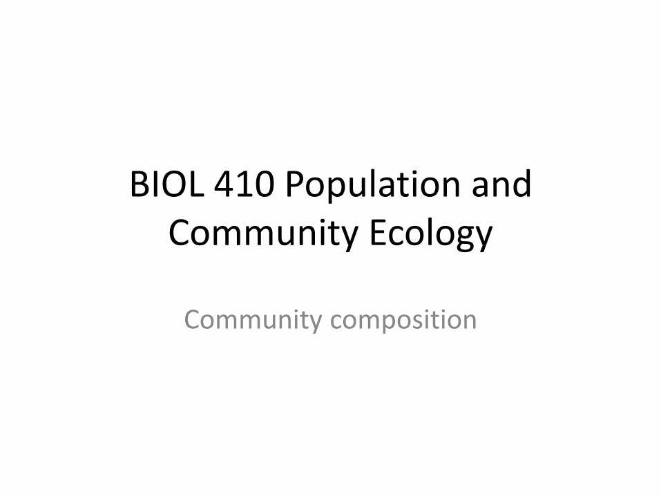
Ecological communities

Species richness (number of species)

Questions of ecological communities

• For a given community, how many species are present and what are their relative abundances?

• How many species are rare?

• How many species are common?

• How can the species in the community be grouped

• What type of interactions occur between the species groups (guilds)?

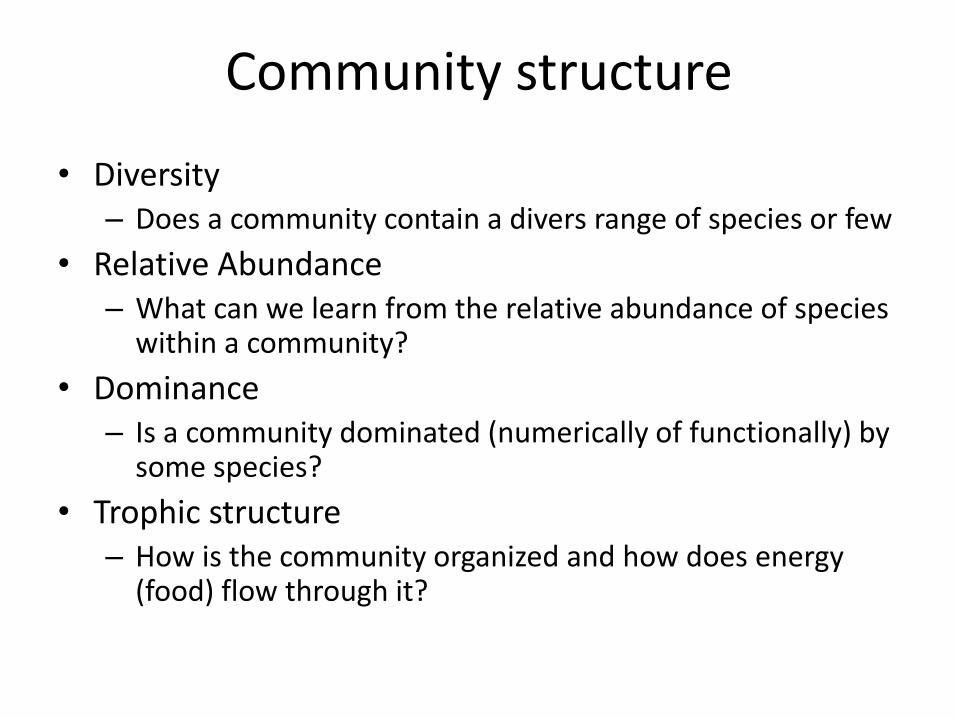
Community structure

• Diversity – Does a community contain a divers range of species or few

• Relative Abundance – What can we learn from the relative abundance of species

within a community?

• Dominance – Is a community dominated (numerically of functionally) by

some species?

• Trophic structure – How is the community organized and how does energy

(food) flow through it?

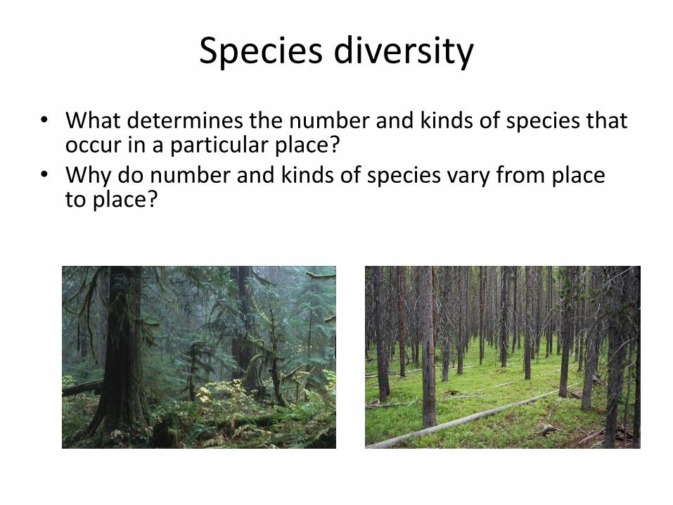
Species diversity

• What determines the number and kinds of species that occur in a particular place?

• Why do number and kinds of species vary from place to place?

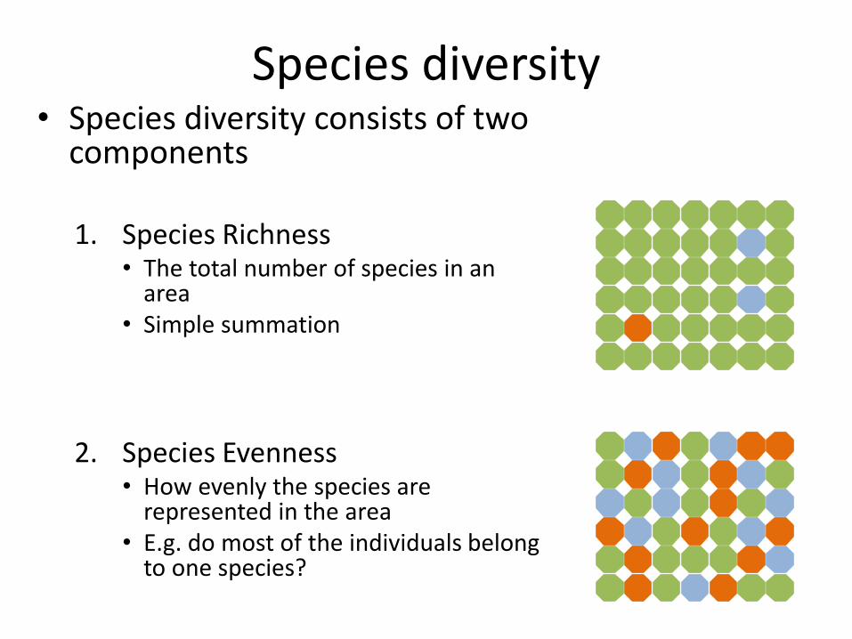
Species diversity • Species diversity consists of two

components 1. Species Richness

• The total number of species in an area

• Simple summation

2. Species Evenness • How evenly the species are

represented in the area • E.g. do most of the individuals belong

to one species?

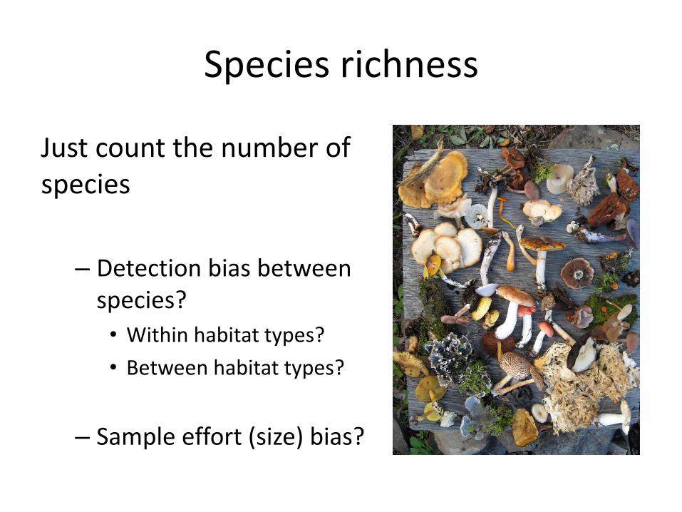
Species richness

Just count the number of species

– Detection bias between species?

• Within habitat types?

• Between habitat types?

– Sample effort (size) bias?

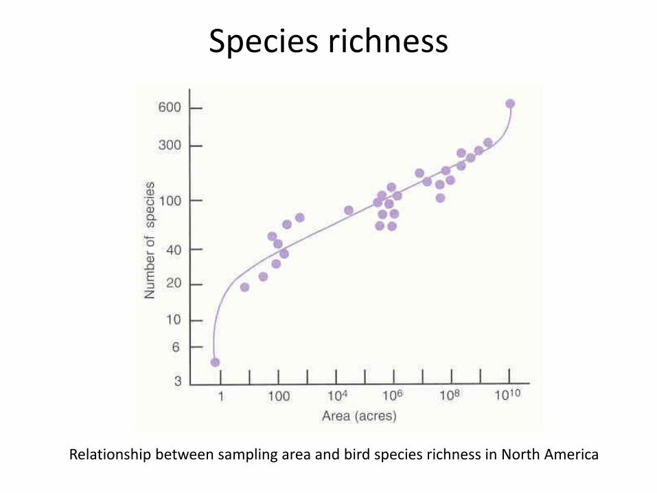
Species richness

Relationship between sampling area and bird species richness in North America

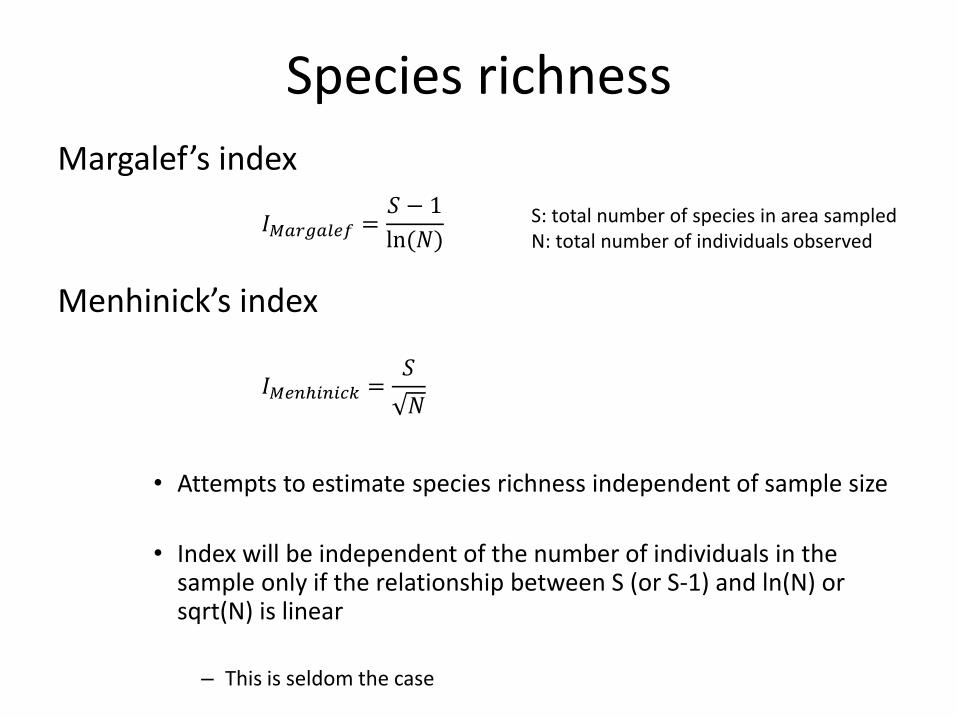
Species richness

Margalef’s index

Menhinick’s index

• Attempts to estimate species richness independent of sample size

• Index will be independent of the number of individuals in the sample only if the relationship between S (or S-1) and ln(N) or sqrt(N) is linear

– This is seldom the case

𝐼𝑀𝑎𝑟𝑔𝑎𝑙𝑒𝑓 =𝑆 − 1

ln(𝑁)

𝐼𝑀𝑒𝑛ℎ𝑖𝑛𝑖𝑐𝑘 =𝑆

𝑁

S: total number of species in area sampled N: total number of individuals observed

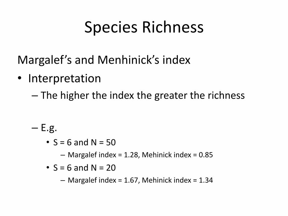
Species Richness

Margalef’s and Menhinick’s index

• Interpretation

– The higher the index the greater the richness

– E.g.

• S = 6 and N = 50 – Margalef index = 1.28, Mehinick index = 0.85

• S = 6 and N = 20 – Margalef index = 1.67, Mehinick index = 1.34

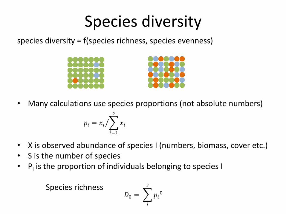
Species diversity species diversity = f(species richness, species evenness)

• Many calculations use species proportions (not absolute numbers)

• X is observed abundance of species I (numbers, biomass, cover etc.) • S is the number of species • Pi is the proportion of individuals belonging to species I

Species richness

𝑝𝑖 = 𝑥𝑖 𝑥𝑖

𝑠

𝑖=1

𝐷0 = 𝑝𝑖0

𝑠

𝑖

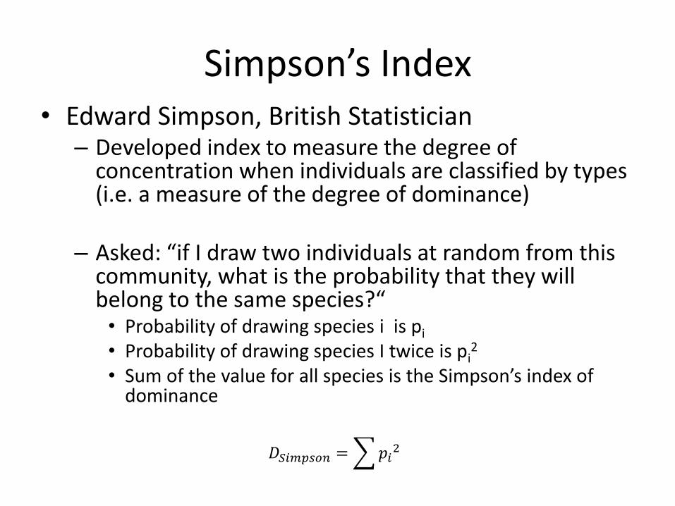
Simpson’s Index • Edward Simpson, British Statistician

– Developed index to measure the degree of concentration when individuals are classified by types (i.e. a measure of the degree of dominance)

– Asked: “if I draw two individuals at random from this community, what is the probability that they will belong to the same species?“

• Probability of drawing species i is pi

• Probability of drawing species I twice is pi2

• Sum of the value for all species is the Simpson’s index of dominance

𝐷𝑆𝑖𝑚𝑝𝑠𝑜𝑛 = 𝑝𝑖2

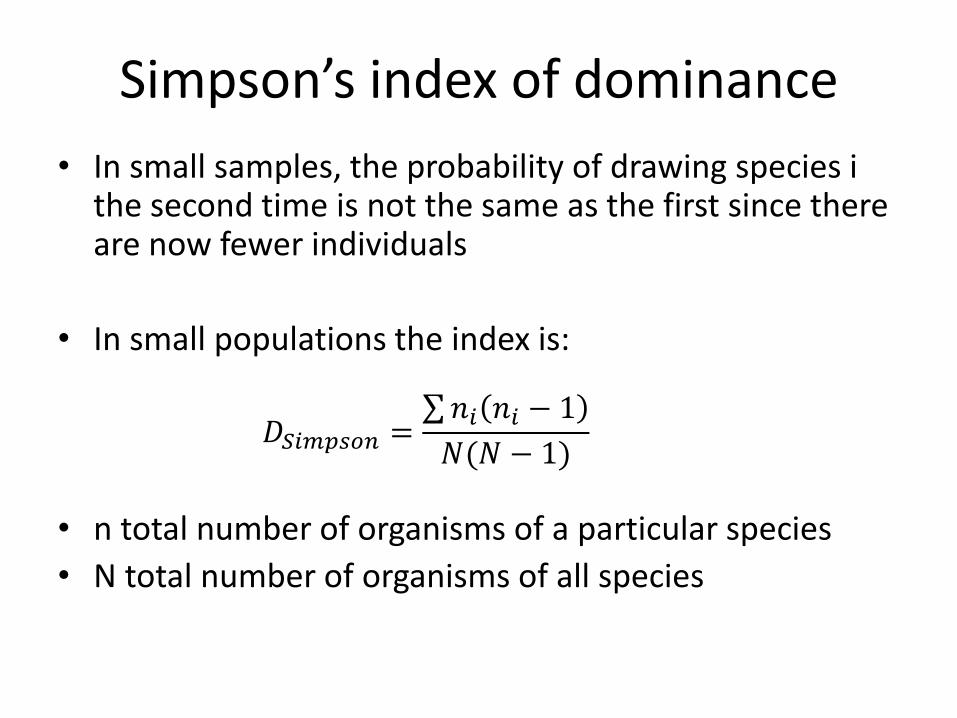
Simpson’s index of dominance

• In small samples, the probability of drawing species i the second time is not the same as the first since there are now fewer individuals

• In small populations the index is:

• n total number of organisms of a particular species

• N total number of organisms of all species

𝐷𝑆𝑖𝑚𝑝𝑠𝑜𝑛 = 𝑛𝑖 𝑛𝑖 − 1

𝑁(𝑁 − 1)

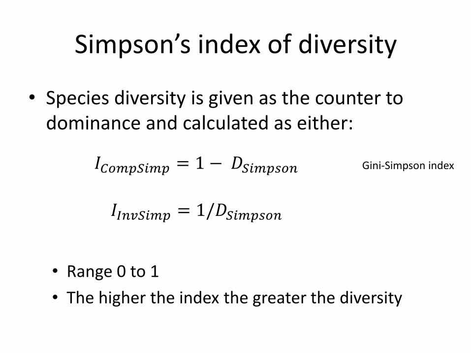
Simpson’s index of diversity

• Species diversity is given as the counter to dominance and calculated as either:

• Range 0 to 1

• The higher the index the greater the diversity

𝐼𝐶𝑜𝑚𝑝𝑆𝑖𝑚𝑝 = 1 −𝐷𝑆𝑖𝑚𝑝𝑠𝑜𝑛

𝐼𝐼𝑛𝑣𝑆𝑖𝑚𝑝 = 1/𝐷𝑆𝑖𝑚𝑝𝑠𝑜𝑛

Gini-Simpson index

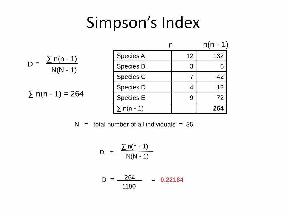
Simpson’s Index

∑ n(n - 1) = 264

D = ∑ n(n - 1)

N(N - 1)

Species A 12 132

Species B 3 6

Species C 7 42

Species D 4 12

Species E 9 72

∑ n(n - 1) 264

n(n - 1) n

D = ∑ n(n - 1)

N(N - 1)

N = total number of all individuals = 35

D = 264

1190 = 0.22184

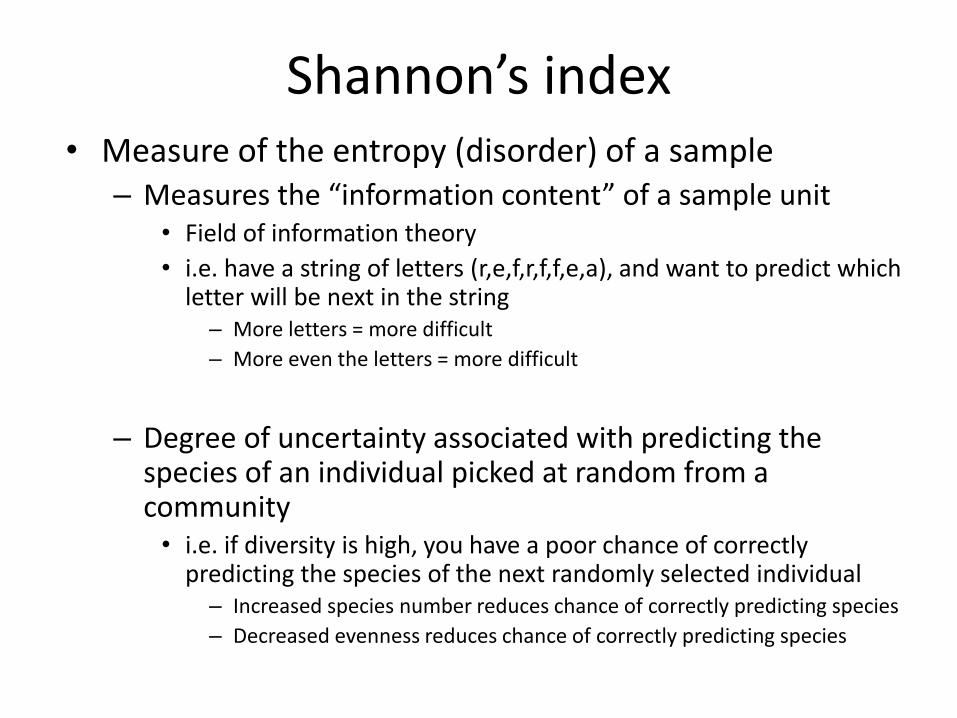
Shannon’s index • Measure of the entropy (disorder) of a sample

– Measures the “information content” of a sample unit • Field of information theory

• i.e. have a string of letters (r,e,f,r,f,f,e,a), and want to predict which letter will be next in the string

– More letters = more difficult

– More even the letters = more difficult

– Degree of uncertainty associated with predicting the species of an individual picked at random from a community

• i.e. if diversity is high, you have a poor chance of correctly predicting the species of the next randomly selected individual

– Increased species number reduces chance of correctly predicting species

– Decreased evenness reduces chance of correctly predicting species

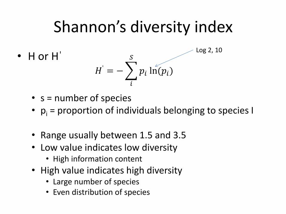
Shannon’s diversity index

• H or Hˈ • s = number of species • pi = proportion of individuals belonging to species I

• Range usually between 1.5 and 3.5 • Low value indicates low diversity

• High information content

• High value indicates high diversity • Large number of species • Even distribution of species

𝐻ˈ = − 𝑝𝑖ln(𝑝𝑖

𝑆

𝑖

)

Log 2, 10

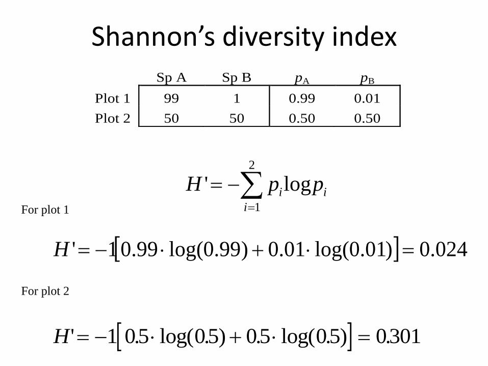
Sp A Sp B pA pB

Plot 1 99 1 0.99 0.01

Plot 2 50 50 0.50 0.50

i

i

i ppH

2

1

log'

024.0)01.0log(01.0)99.0log(99.01' H

H' . log( . ) . log( . ) . 1 05 05 05 05 0301

For plot 1

For plot 2

Shannon’s diversity index

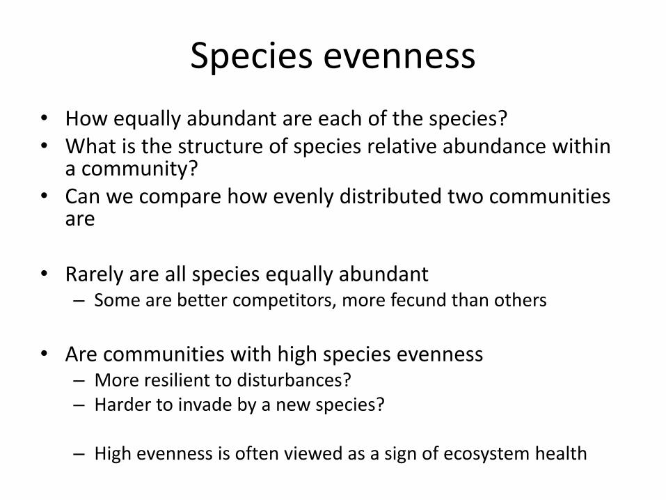
Species evenness

• How equally abundant are each of the species? • What is the structure of species relative abundance within

a community? • Can we compare how evenly distributed two communities

are

• Rarely are all species equally abundant – Some are better competitors, more fecund than others

• Are communities with high species evenness

– More resilient to disturbances? – Harder to invade by a new species?

– High evenness is often viewed as a sign of ecosystem health

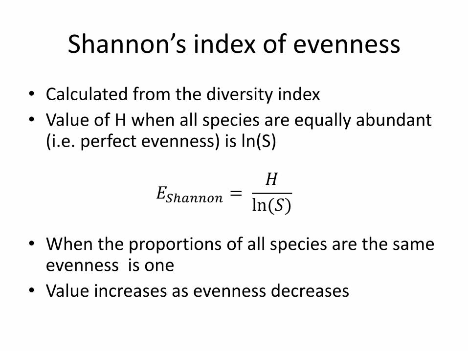
Shannon’s index of evenness

• Calculated from the diversity index

• Value of H when all species are equally abundant (i.e. perfect evenness) is ln(S)

• When the proportions of all species are the same evenness is one

• Value increases as evenness decreases

𝐸𝑆ℎ𝑎𝑛𝑛𝑜𝑛 =𝐻

ln(𝑆)

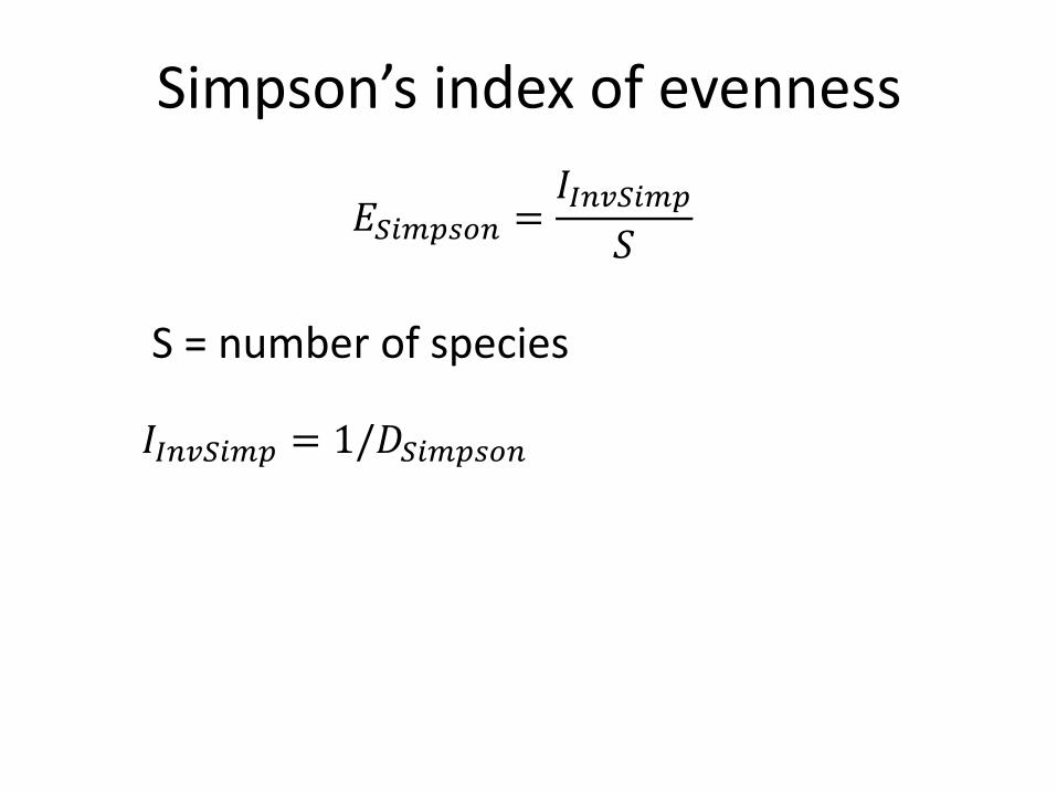
Simpson’s index of evenness

S = number of species

𝐸𝑆𝑖𝑚𝑝𝑠𝑜𝑛 =𝐼𝐼𝑛𝑣𝑆𝑖𝑚𝑝

𝑆

𝐼𝐼𝑛𝑣𝑆𝑖𝑚𝑝 = 1/𝐷𝑆𝑖𝑚𝑝𝑠𝑜𝑛

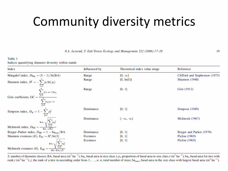
Community diversity metrics

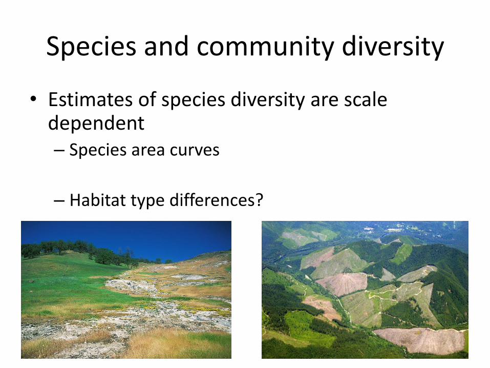
Species and community diversity

• Estimates of species diversity are scale dependent – Species area curves

– Habitat type differences?

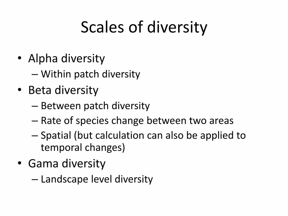
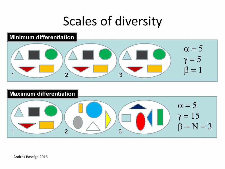
Scales of diversity

• Alpha diversity – Within patch diversity

• Beta diversity – Between patch diversity

– Rate of species change between two areas

– Spatial (but calculation can also be applied to temporal changes)

• Gama diversity – Landscape level diversity

Scales of diversity

Andres Baselga 2015

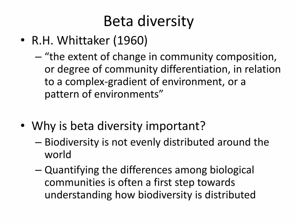
Beta diversity • R.H. Whittaker (1960)

– “the extent of change in community composition, or degree of community differentiation, in relation to a complex-gradient of environment, or a pattern of environments”

• Why is beta diversity important? – Biodiversity is not evenly distributed around the

world

– Quantifying the differences among biological communities is often a first step towards understanding how biodiversity is distributed

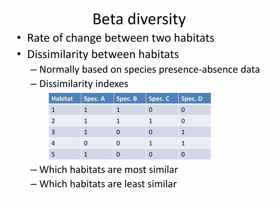
Beta diversity • Rate of change between two habitats

• Dissimilarity between habitats – Normally based on species presence-absence data

– Dissimilarity indexes

– Which habitats are most similar

– Which habitats are least similar

Habitat Spec. A Spec. B Spec. C Spec. D

1 1 1 0 0

2 1 1 1 0

3 1 0 0 1

4 0 0 1 1

5 1 0 0 0

Beta diversity

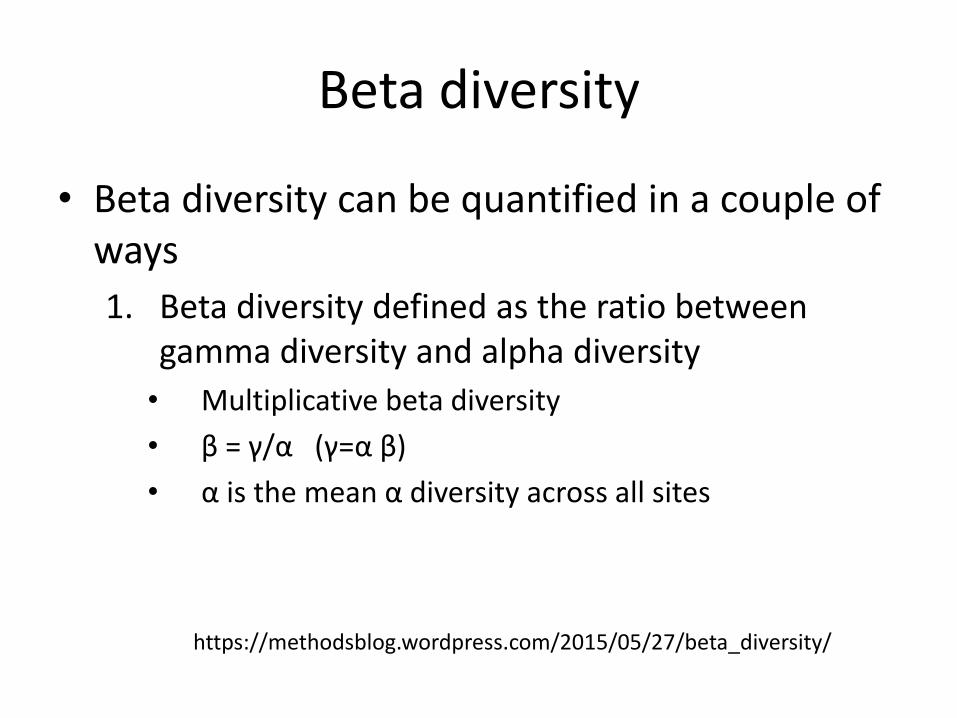
• Beta diversity can be quantified in a couple of ways

1. Beta diversity defined as the ratio between gamma diversity and alpha diversity

• Multiplicative beta diversity

• β = γ/α (γ=α β)

• α is the mean α diversity across all sites

https://methodsblog.wordpress.com/2015/05/27/beta_diversity/

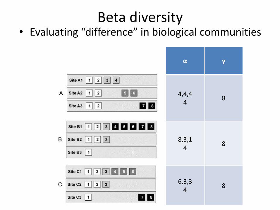
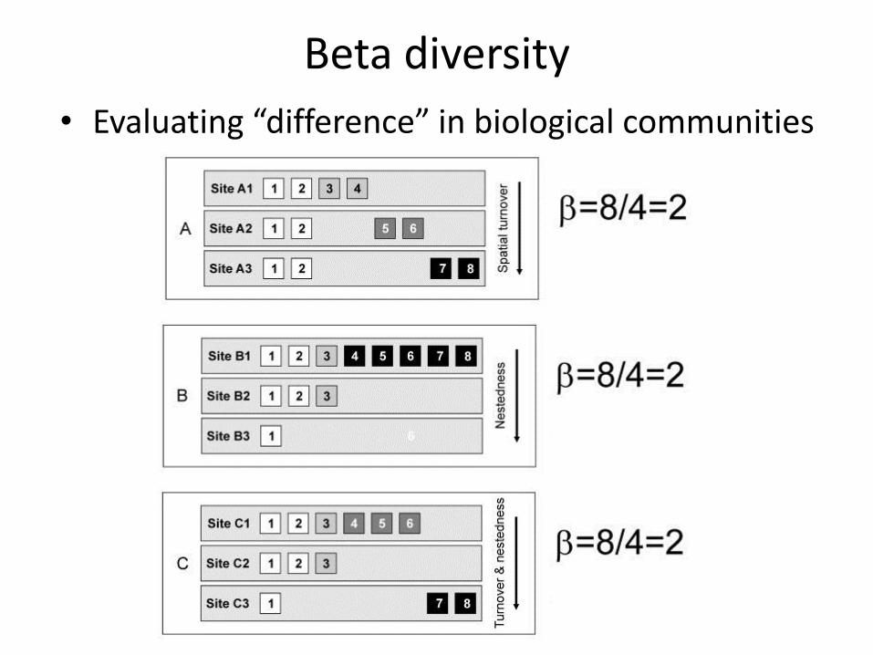
Beta diversity • Evaluating “difference” in biological communities

α γ

4,4,4 4

8

8,3,1 4

8

6,3,3 4

8

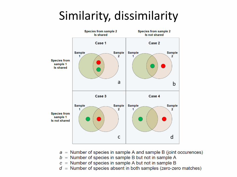
Similarity, dissimilarity

a b

c d

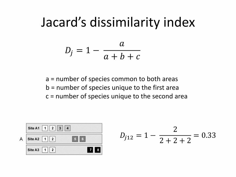
Jacard’s dissimilarity index

a = number of species common to both areas b = number of species unique to the first area c = number of species unique to the second area

𝐷𝑗 = 1 −𝑎

𝑎 + 𝑏 + 𝑐

𝐷𝑗12 = 1 −2

2 + 2 + 2= 0.33

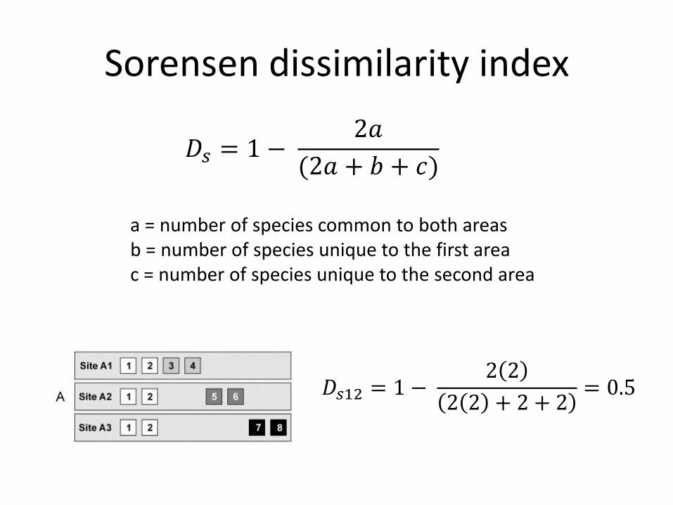
Sorensen dissimilarity index

a = number of species common to both areas b = number of species unique to the first area c = number of species unique to the second area

𝐷𝑠 = 1 −2𝑎

(2𝑎 + 𝑏 + 𝑐)

𝐷𝑠12 = 1 −2 2

2 2 + 2 + 2= 0.5

Beta diversity

• Evaluating “difference” in biological communities

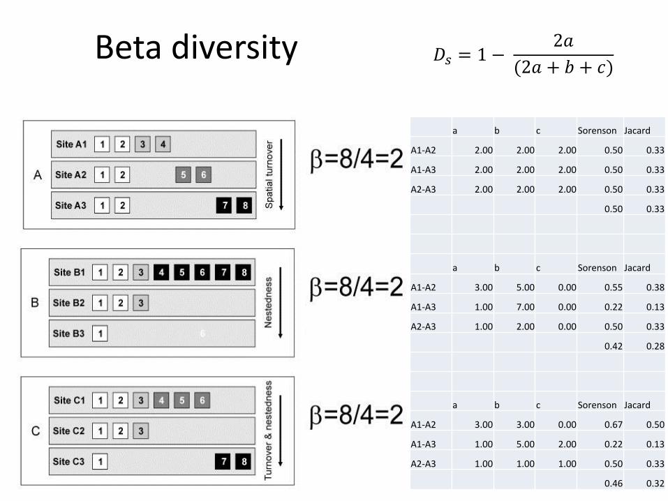
Beta diversity

a b c Sorenson Jacard

A1-A2 2.00 2.00 2.00 0.50 0.33

A1-A3 2.00 2.00 2.00 0.50 0.33

A2-A3 2.00 2.00 2.00 0.50 0.33

0.50 0.33

a b c Sorenson Jacard

A1-A2 3.00 5.00 0.00 0.55 0.38

A1-A3 1.00 7.00 0.00 0.22 0.13

A2-A3 1.00 2.00 0.00 0.50 0.33

0.42 0.28

a b c Sorenson Jacard

A1-A2 3.00 3.00 0.00 0.67 0.50

A1-A3 1.00 5.00 2.00 0.22 0.13

A2-A3 1.00 1.00 1.00 0.50 0.33

0.46 0.32

𝐷𝑠 = 1 −2𝑎

(2𝑎 + 𝑏 + 𝑐)