Interactive Analysis of Large-Scale Sequencing Genomics Data Sets using a Real-Time Distributed Database

Hans-Martin Will, Ph.D., Dominic Suciu, Ph.D. – SpaceCurve, Seattle, WA, USA

SpaceCurve | 710 Second Avenue #620, Seattle, WA 98104 | spacecurve.com | hm@spacecurve.com

Conclusions!We have shown the feasibility of storing high-throughput sequencing data fully schematized and indexed at the level of individual reads within a next-generation Big Data platform, thereby providing an attractive alternative to file based informatics pipelines. While we have conducted our study within a single framework for variation analysis, we believe that the ability to quickly create analysis data sets across studies and genomic regions applies to many other analysis methodologies as well. We see the following areas for future work: 1.) Improving the overall storage efficiency using better data representation and compression techniques. 2.) Providing a more natural representation of genomic locations at the SQL level.

Introduction!With the arrival of the $1,000 human genome, the dream and promise of applying high-throughput sequencing (HTS) to large populations has come true. However, as described elsewhere [1], the complexity and cost of managing the generated data and performing computation effectively for their analysis and interpretation have become the major challenge and dominating cost factor. Currently, the most workable approach to handling these data sets is organizing sequencing data in the form of many individual data files that are stored in distributed storage clusters or cloud storage. Bioinformatics pipelines that analyze those data sets are then implemented using distributed file-based batch-processing engines, such as Apache Hadoop (MapReduce) or the Open Grid Scheduler (formerly Sun Grid Engine). In such an approach, turn-around time of creating and running new batch jobs becomes the limiting factor during data analysis. Ultimately, this leads to a situation where researchers find themselves hampered in their ability to ask “what if?” questions not due to lack of creativity or availability of data but due to mere processing time and inconvenience.   In recent years, driven by the needs of mobile analytics and the Internet of Things, a new generation of Big Data technology has been developed that provides multi-dimensional indexing capabilities at scale. Examples are Postgres-XC [2], SAP HANA with Spatial Processing [3], or the SpaceCurve data platform [4] used here. In this poster, we describe our experience of applying such a next-generation storage engine to the problem of characterizing genetic variation in high-throughput sequencing data. Our particular analysis is motivated by the framework described in DePristo et al. (2011) [5] and aims to model the relevant data access patterns.

Materials and Methods!Data!For our study we chose the 1000 Genomes data set [6] published via Amazon Web Services (AWS) [7]. Specifically, we started with the complete set of aligned reads that are provided in the form of BAM [8] files across all 1092 individuals included in the study. Those BAM files amount to 35 TB of data. Spatial Mapping!We are using database capabilities defined by the spatial extensions to the SQL standard [9]. Each aligned read is mapped into a 2-dimensional space and represented as a SQL LINESTRING object. The x-axis used for this mapping is a linearization of all chromosomes making up the genome. That is, location P on chromosome C is mapped to an x-coordinate

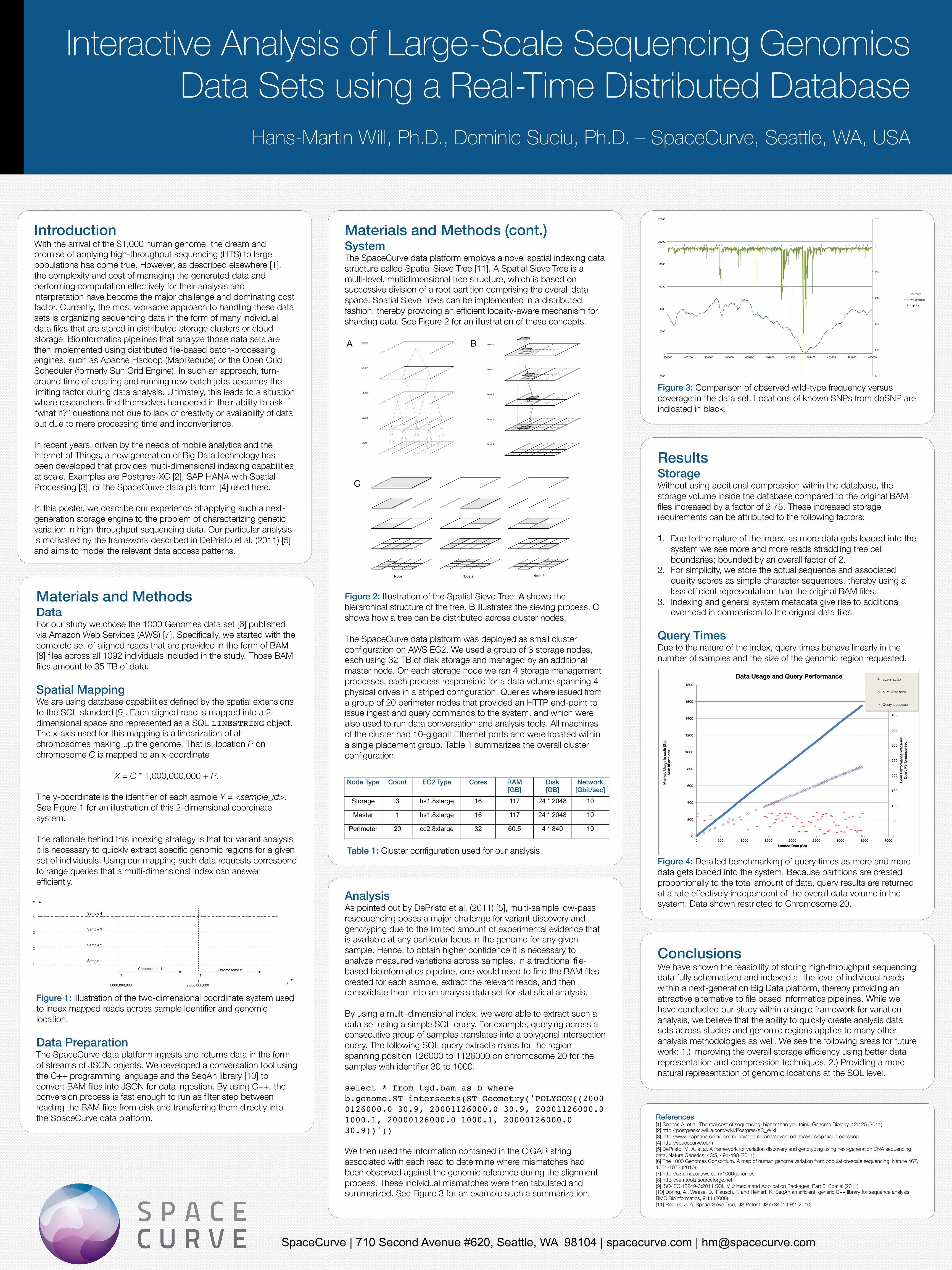
X = C * 1,000,000,000 + P. The y-coordinate is the identifier of each sample Y = <sample_id>. See Figure 1 for an illustration of this 2-dimensional coordinate system. The rationale behind this indexing strategy is that for variant analysis it is necessary to quickly extract specific genomic regions for a given set of individuals. Using our mapping such data requests correspond to range queries that a multi-dimensional index can answer efficiently. Figure 1: Illustration of the two-dimensional coordinate system used to index mapped reads across sample identifier and genomic location. Data Preparation!The SpaceCurve data platform ingests and returns data in the form of streams of JSON objects. We developed a conversation tool using the C++ programming language and the SeqAn library [10] to convert BAM files into JSON for data ingestion. By using C++, the conversion process is fast enough to run as filter step between reading the BAM files from disk and transferring them directly into the SpaceCurve data platform.

References![1] Sboner, A. et al. The real cost of sequencing: higher than you think! Genome Biology, 12:125 (2011) [2] http://postgresxc.wikia.com/wiki/Postgres-XC_Wiki [3] http://www.saphana.com/community/about-hana/advanced-analytics/spatial-processing [4] http://spacecurve.com [5] DePristo, M. A. et al, A framework for variation discovery and genotyping using next-generation DNA sequencing data, Nature Genetics, 43:5, 491-498 (2011) [6] The 1000 Genomes Consortium. A map of human genome variation from population-scale sequencing. Nature 467, 1061-1073 (2010) [7] http://s3.amazonaws.com/1000genomes [8] http://samtools.sourceforge.net [9] ISO/IEC 13249-3:2011 SQL Multimedia and Application Packages, Part 3: Spatial (2011) [10] Döring, A., Weese, D., Rausch, T. and Reinert, K. SeqAn an efficient, generic C++ library for sequence analysis. BMC Bioinformatics, 9:11 (2008) [11] Rogers, J. A. Spatial Sieve Tree, US Patent US7734714 B2 (2010)

Materials and Methods (cont.)!System!The SpaceCurve data platform employs a novel spatial indexing data structure called Spatial Sieve Tree [11]. A Spatial Sieve Tree is a multi-level, multidimensional tree structure, which is based on successive division of a root partition comprising the overall data space. Spatial Sieve Trees can be implemented in a distributed fashion, thereby providing an efficient locality-aware mechanism for sharding data. See Figure 2 for an illustration of these concepts. Figure 2: Illustration of the Spatial Sieve Tree: A shows the hierarchical structure of the tree. B illustrates the sieving process. C shows how a tree can be distributed across cluster nodes. The SpaceCurve data platform was deployed as small cluster configuration on AWS EC2. We used a group of 3 storage nodes, each using 32 TB of disk storage and managed by an additional master node. On each storage node we ran 4 storage management processes, each process responsible for a data volume spanning 4 physical drives in a striped configuration. Queries where issued from a group of 20 perimeter nodes that provided an HTTP end-point to issue ingest and query commands to the system, and which were also used to run data conversation and analysis tools. All machines of the cluster had 10-gigabit Ethernet ports and were located within a single placement group. Table 1 summarizes the overall cluster configuration.  Table 1: Cluster configuration used for our analysis

Chromosome 1 Chromosome 2

Sample 1

Sample 2

Sample 3

1 1

1,000,000,000 2,000,000,000

1

2

3

4

Y

X

Sample 4

Node Type! Count! EC2 Type! Cores! RAM ![GB]!

Disk![GB]!

Network [Gbit/sec]!

Storage 3 hs1.8xlarge 16 117 24 * 2048 10

Master 1 hs1.8xlarge 16 117 24 * 2048 10

Perimeter 20 cc2.8xlarge 32 60.5 4 * 840 10

Level 0

Level 1

Level 2

Level 3

Level 4

Level 0

Level 1

Level 2

Level 3

Level 4

Node 1 Node 2 Node 3

C

A B

!!!!!!!!!!!!!!!Figure 3: Comparison of observed wild-type frequency versus coverage in the data set. Locations of known SNPs from dbSNP are indicated in black.

Results!Storage!Without using additional compression within the database, the storage volume inside the database compared to the original BAM files increased by a factor of 2.75. These increased storage requirements can be attributed to the following factors: 1.  Due to the nature of the index, as more data gets loaded into the

system we see more and more reads straddling tree cell boundaries; bounded by an overall factor of 2.

2.  For simplicity, we store the actual sequence and associated quality scores as simple character sequences, thereby using a less efficient representation than the original BAM files.

3.  Indexing and general system metadata give rise to additional overhead in comparison to the original data files.

!Query Times!Due to the nature of the index, query times behave linearly in the number of samples and the size of the genomic region requested. !!!!!!!!!!!!!!!!!!Figure 4: Detailed benchmarking of query times as more and more data gets loaded into the system. Because partitions are created proportionally to the total amount of data, query results are returned at a rate effectively independent of the overall data volume in the system. Data shown restricted to Chromosome 20.

Analysis!As pointed out by DePristo et al. (2011) [5], multi-sample low-pass resequencing poses a major challenge for variant discovery and genotyping due to the limited amount of experimental evidence that is available at any particular locus in the genome for any given sample. Hence, to obtain higher confidence it is necessary to analyze measured variations across samples. In a traditional file-based bioinformatics pipeline, one would need to find the BAM files created for each sample, extract the relevant reads, and then consolidate them into an analysis data set for statistical analysis. By using a multi-dimensional index, we were able to extract such a data set using a simple SQL query. For example, querying across a consecutive group of samples translates into a polygonal intersection query. The following SQL query extracts reads for the region spanning position 126000 to 1126000 on chromosome 20 for the samples with identifier 30 to 1000. select * from tgd.bam as b where b.genome.ST_intersects(ST_Geometry('POLYGON((20000126000.0 30.9, 20001126000.0 30.9, 20001126000.0 1000.1, 20000126000.0 1000.1, 20000126000.0 30.9))'))! We then used the information contained in the CIGAR string associated with each read to determine where mismatches had been observed against the genomic reference during the alignment process. These individual mismatches were then tabulated and summarized. See Figure 3 for an example such a summarization.

0!

50!

100!

150!

200!

250!

300!

350!

400!

450!

500!

0!

200!

400!

600!

800!

1000!

1200!

1400!

1600!

1800!

0! 500! 1000! 1500! 2000! 2500! 3000! 3500! 4000!

Loa

d Pe

rform

ance

kre

cs/s

ec!

Que

ry P

erfo

rman

ce s

ec!

Mem

ory

Usag

e in

scd

b (G

b)!

Num

kPa

rtitio

ns!

Loaded Data (Gb)!

Data Usage and Query Performance !size in scdb

num kPartitions

Query krecs/sec

0"

0.2"

0.4"

0.6"

0.8"

1"

1.2"

)2000"

0"

2000"

4000"

6000"

8000"

10000"

12000"

400000" 400200" 400400" 400600" 400800" 401000" 401200" 401400" 401600" 401800" 402000"

coverage"

wt/coverage"

snp_loc"