Embed Size (px)
Citation preview
Bioinformática: Inferência filogenética
WHYDO WE CARE ?
Rita Castilho, [email protected]
What for?
Forense
Prever a evolução do vírus da influenza
Prevêr as funções de genes não caracterizados
Descoberta de drogas
Desenvolvimento de vacinas
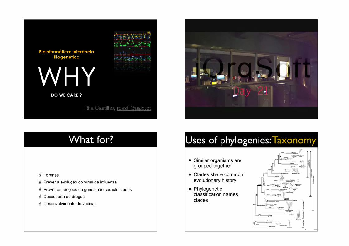
Uses of phylogenies: Taxonomy
• Similar organisms are grouped together
• Clades share common evolutionary history
• Phylogenetic classification names clades
Source: Inoue, J.G., Miya, M., Tsukamoto, K., Nishida, M. 2003.
Basal actinopterygian relationships: a mitogenomic perspective on the
phylogeny of the “ancient fish”. Molecular Phylogenetics and
Evolution, 26: 110-120.
Pryer et al. 2001
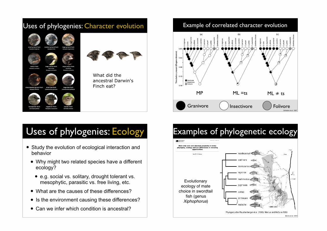
Uses of phylogenies: Character evolution
What did the ancestral Darwin's Finch eat?
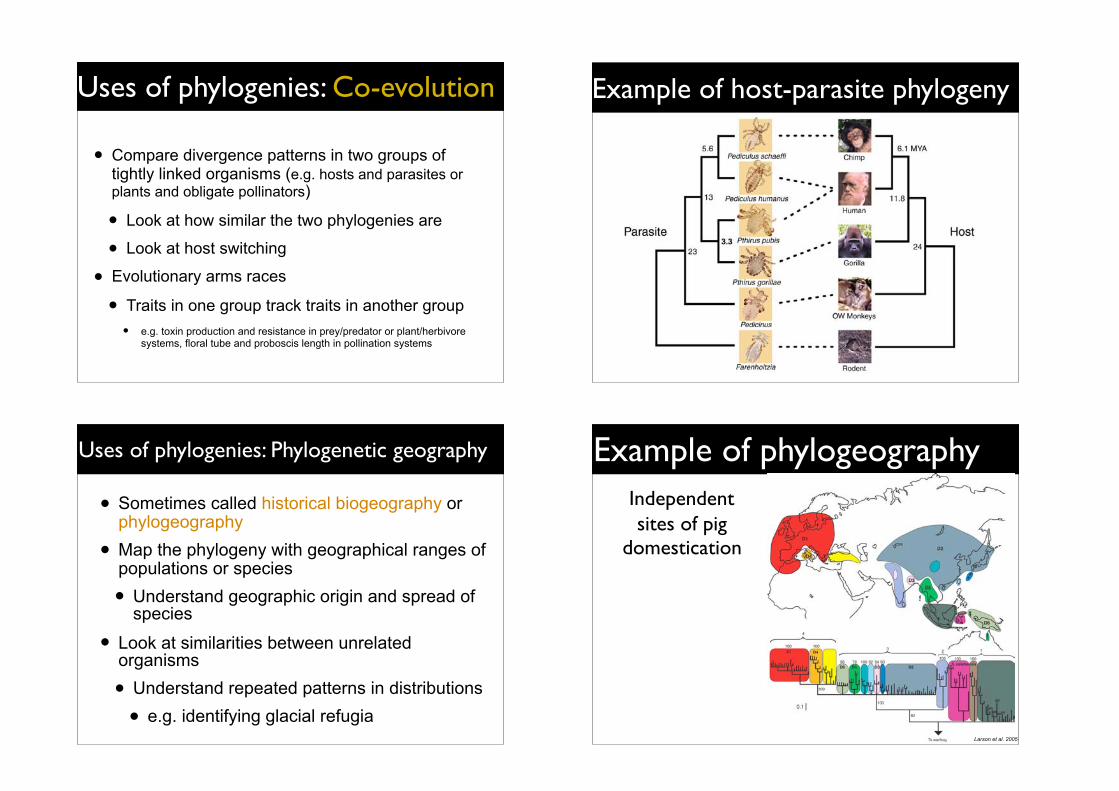
Example of correlated character evolution
Granivore Insectivore Folivore
MP ML =ts ML ≠ ts
Schluter et al. 1997
Uses of phylogenies: Ecology
• Study the evolution of ecological interaction and behavior
• Why might two related species have a different ecology?
• e.g. social vs. solitary, drought tolerant vs. mesophytic, parasitic vs. free living, etc.
• What are the causes of these differences?
• Is the environment causing these differences?
• Can we infer which condition is ancestral?
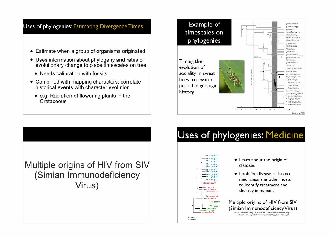
Examples of phylogenetic ecology
Evolutionary ecology of mate
choice in swordtail fish (genus Xiphophorus)
Morris et al. 2003
Uses of phylogenies: Co-evolution
• Compare divergence patterns in two groups of tightly linked organisms (e.g. hosts and parasites or plants and obligate pollinators)
• Look at how similar the two phylogenies are
• Look at host switching
• Evolutionary arms races
• Traits in one group track traits in another group • e.g. toxin production and resistance in prey/predator or plant/herbivore
systems, floral tube and proboscis length in pollination systems
Example of host-parasite phylogeny
Uses of phylogenies: Phylogenetic geography
• Sometimes called historical biogeography or phylogeography
• Map the phylogeny with geographical ranges of populations or species
• Understand geographic origin and spread of species
• Look at similarities between unrelated organisms
• Understand repeated patterns in distributions
• e.g. identifying glacial refugia
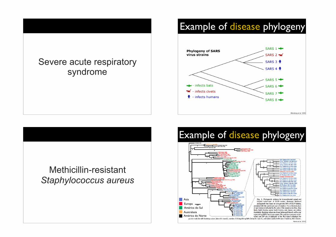
Example of phylogeographyIndependent sites of pig
domestication
Larson et al. 2005
Uses of phylogenies: Estimating Divergence Times
• Estimate when a group of organisms originated
• Uses information about phylogeny and rates of evolutionary change to place timescales on tree
• Needs calibration with fossils
• Combined with mapping characters, correlate historical events with character evolution
• e.g. Radiation of flowering plants in the Cretaceous
Example of timescales on phylogenies
Timing the evolution of sociality in sweat bees to a warm period in geologic history
Brady et al. 2006
Multiple origins of HIV from SIV (Simian Immunodeficiency
Virus)
Uses of phylogenies: Medicine
• Learn about the origin of diseases
• Look for disease resistance mechanisms in other hosts to identify treatment and therapy in humans
Multiple origins of HIV from SIV (Simian Immunodeficiency Virus)
From: Understanding Evolution. HIV: the ultimate evolver. http://evolution.berkeley.edu/evolibrary/article/0_0_0/medicine_04
Severe acute respiratory syndrome
Example of disease phylogeny
Wendong et al. 2005
Methicillin-resistant Staphylococcus aureus
Asia
EuropaAmérica do Sul
AustralasiaAmérica do Norte
Example of disease phylogeny
Harris et al. 2010
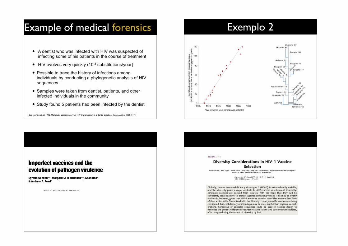
Example of medical forensics
• A dentist who was infected with HIV was suspected of infecting some of his patients in the course of treatment
• HIV evolves very quickly (10-3 substitutions/year)
• Possible to trace the history of infections among individuals by conducting a phylogenetic analysis of HIV sequences
• Samples were taken from dentist, patients, and other infected individuals in the community
• Study found 5 patients had been infected by the dentist
Source: Ou et. al. 1992. Molecular epidemiology of HIV transmission in a dental practice. Science, 256: 1165-1171.
Exemplo 2
Filogenia e evolução molecular
Rita Castilho, [email protected]
=
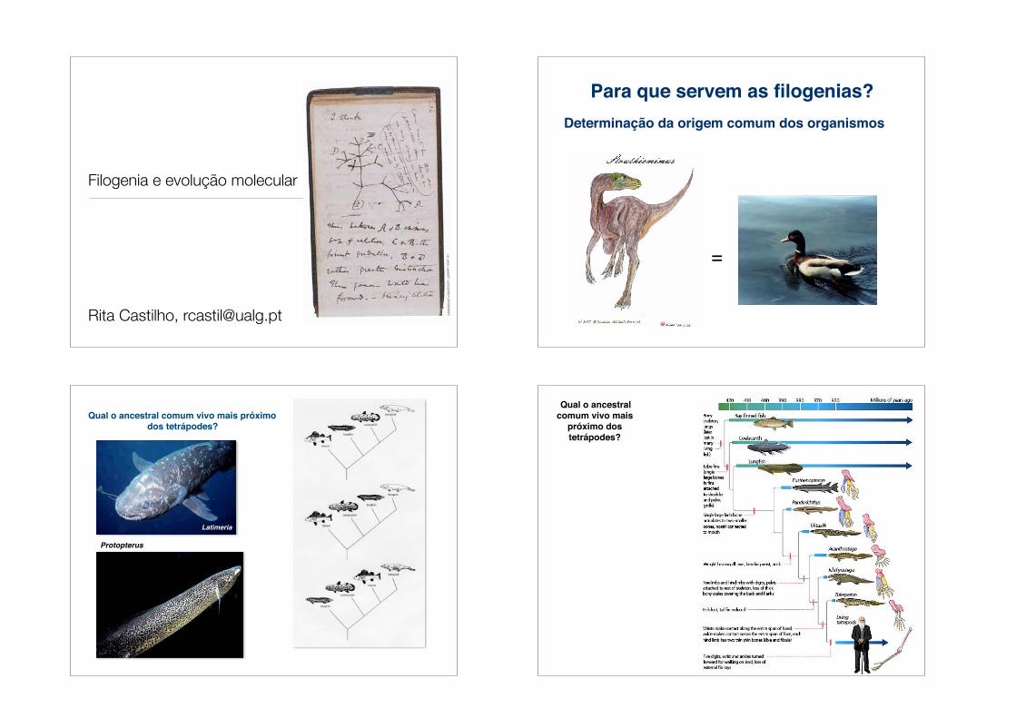
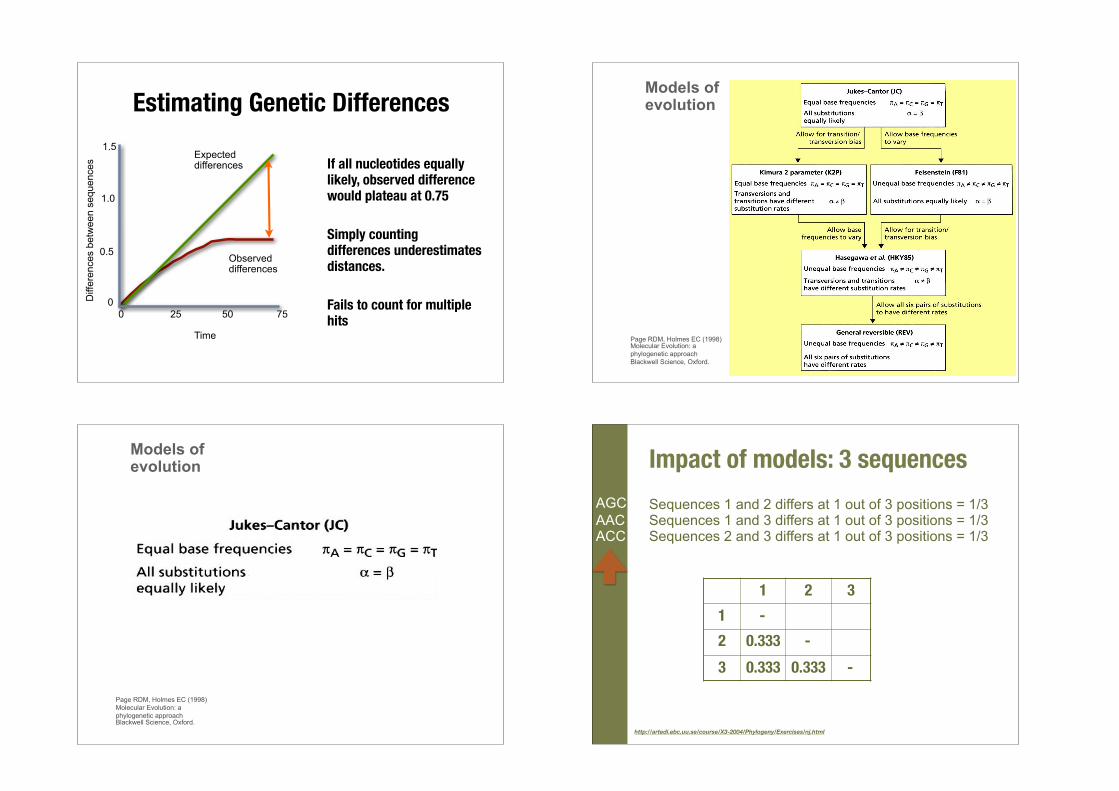
Determinação da origem comum dos organismos
Para que servem as filogenias?
Latimeria
Protopterus
Qual o ancestral comum vivo mais próximo dos tetrápodes?
Qual o ancestral comum vivo mais
próximo dos tetrápodes?
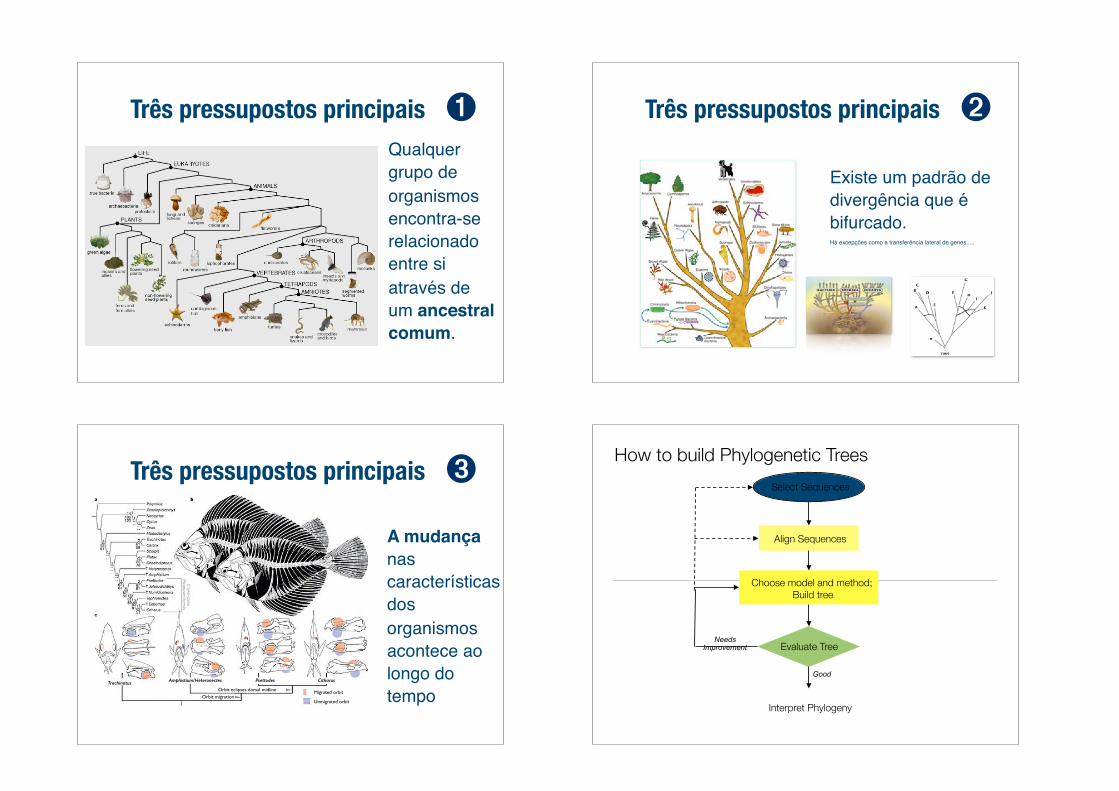
Três pressupostos principaisQualquer grupo de organismos encontra-se relacionado entre si através de um ancestral comum.
➊
Existe um padrão de divergência que é bifurcado.Há excepções como a transferência lateral de genes.....
Três pressupostos principais ➋
A mudança nas características dos organismos acontece ao longo do tempoOrbit eclipses dorsal midline
Orbit migration
CitharusPsettodesAmphistium/HeteronectesTrachinatus
Migrated orbit
Unmigrated orbit
Três pressupostos principais ➌How to build Phylogenetic Trees
Select Sequences
Align Sequences
Choose model and method; Build tree
Evaluate Tree
Interpret Phylogeny
Good
Needs Improvement
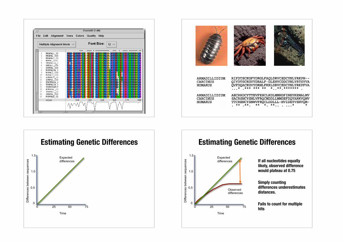
Estimating Genetic Differences
0 25 50 750
0.5
1.0
1.5 Expected differences
Time
Diff
eren
ces
betw
een
sequ
ence
s
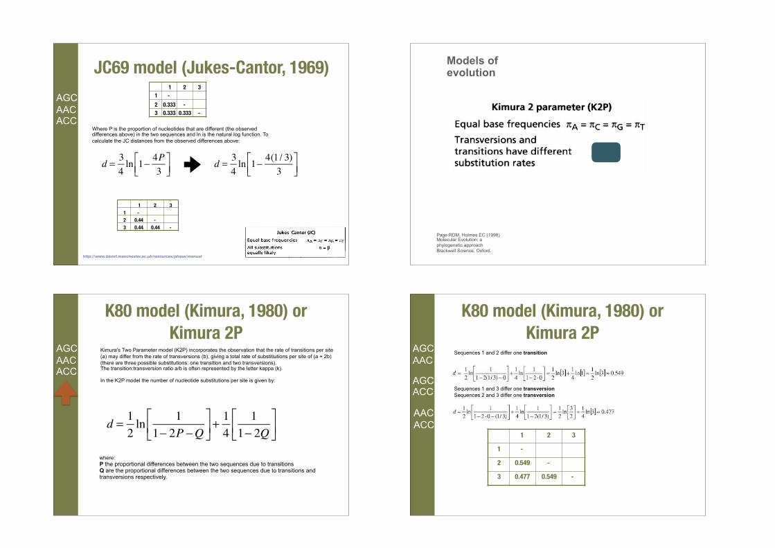
Estimating Genetic Differences
If all nucleotides equally likely, observed difference would plateau at 0.75
Simply counting differences underestimates distances.
Fails to count for multiple hits 0 25 50 75
0
0.5
1.0
1.5 Expected differences
Observed differences
Time
Diff
eren
ces
betw
een
sequ
ence
s
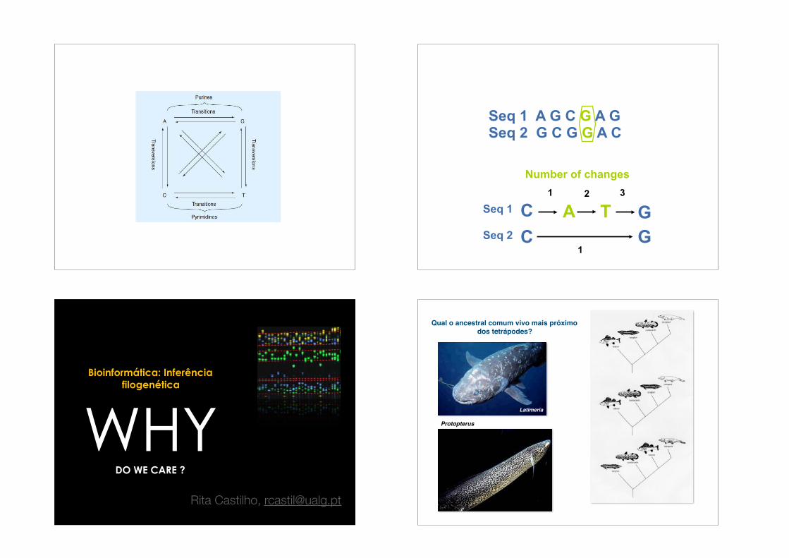
C GC A T G
1 2 3
1
Seq 1
Seq 2
Number of changes
Seq 1 A G C G A G Seq 2 G C G G A C
Bioinformática: Inferência filogenética
WHYDO WE CARE ?
Rita Castilho, [email protected]
Latimeria
Protopterus
Qual o ancestral comum vivo mais próximo dos tetrápodes?

Qual o ancestral comum vivo mais
próximo dos tetrápodes?
One substitutions happened - one substitution is visible
G
CG
PAST
G
CA
PAST
Two substitutions happened - only one substitution is visible Two substitutions happened - no visible substitution
GPAST
A A
Estimating Genetic Differences
If all nucleotides equally likely, observed difference would plateau at 0.75
Simply counting differences underestimates distances.
Fails to count for multiple hits 0 25 50 75
0
0.5
1.0
1.5Expected differences
Observed differences
Time
Diff
eren
ces
betw
een
sequ
ence
s
Page RDM, Holmes EC (1998) Molecular Evolution: a phylogenetic approach Blackwell Science, Oxford.
Models of evolution
Page RDM, Holmes EC (1998) Molecular Evolution: a phylogenetic approach Blackwell Science, Oxford.
Models of evolution Impact of models: 3 sequences
http://artedi.ebc.uu.se/course/X3-2004/Phylogeny/Exercises/nj.html
AGC AAC ACC
Sequences 1 and 2 differs at 1 out of 3 positions = 1/3 Sequences 1 and 3 differs at 1 out of 3 positions = 1/3 Sequences 2 and 3 differs at 1 out of 3 positions = 1/3
1 2 31 -2 0.333 -3 0.333 0.333 -
JC69 model (Jukes-Cantor, 1969)
http://www.bioinf.manchester.ac.uk/resources/phase/manual
Where P is the proportion of nucleotides that are different (the observed differences above) in the two sequences and ln is the natural log function. To calculate the JC distances from the observed differences above:
1 2 31 -2 0.333 -3 0.333 0.333 -
1 2 31 -2 0.44 -3 0.44 0.44 -
AGC AAC ACC
d = 34ln 1− 4P
3⎡⎣⎢
⎤⎦⎥
d = 34ln 1− 4(1 / 3)
3⎡⎣⎢
⎤⎦⎥
Page RDM, Holmes EC (1998) Molecular Evolution: a phylogenetic approach Blackwell Science, Oxford.
Models of evolution
K80 model (Kimura, 1980) orKimura 2P
Kimura's Two Parameter model (K2P) incorporates the observation that the rate of transitions per site (a) may differ from the rate of transversions (b), giving a total rate of substitiutions per site of (a + 2b)(there are three possible substitutions: one transition and two transversions). The transition:transversion ratio a/b is often represented by the letter kappa (k).
In the K2P model the number of nucleotide substitutions per site is given by:
where: P the proportional differences between the two sequences due to transitions Q are the proportional differences between the two sequences due to transitions and transversions respectively.
AGC AAC ACC
d = 12ln 11− 2P −Q⎡⎣⎢
⎤⎦⎥+ 14
11− 2Q⎡⎣⎢
⎤⎦⎥
K80 model (Kimura, 1980) orKimura 2P
Sequences 1 and 3 differ one transversion Sequences 2 and 3 differ one transversion
AGC AAC
Sequences 1 and 2 differ one transition
AGC ACC
AAC ACC
1 2 3
1 -
2 0.549 -
3 0.477 0.549 -
1 2 3
1 -
2 0.549 -
3 0.477 0.549 -
1 2 3
1 -
2 0.441 -
3 0.441 0.441 -
1 2 3
1 -
2 0.333 -
3 0.333 0.333 -
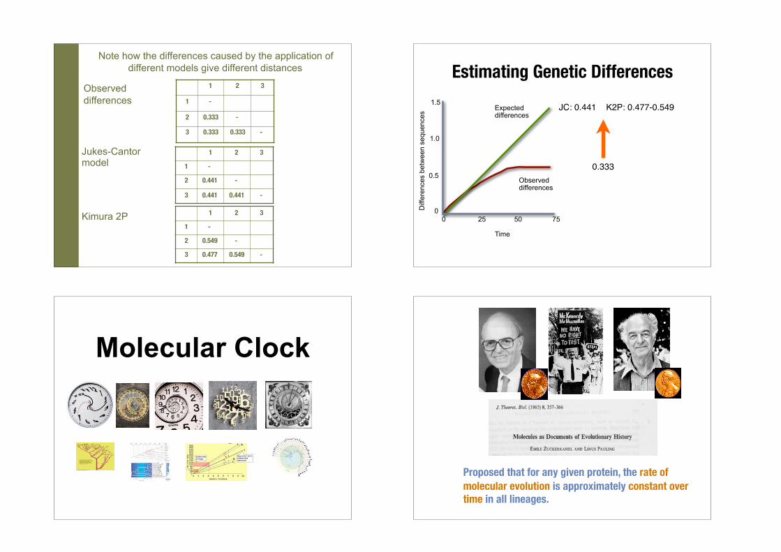
Observed differences
Jukes-Cantor model
Kimura 2P
Note how the differences caused by the application of different models give different distances Estimating Genetic Differences
0 25 50 750
0.5
1.0
1.5Expected differences
Observed differences
Time
Diff
eren
ces
betw
een
sequ
ence
s
0.333
JC: 0.441 K2P: 0.477-0.549
Molecular Clock
Proposed that for any given protein, the rate of molecular evolution is approximately constant over time in all lineages.
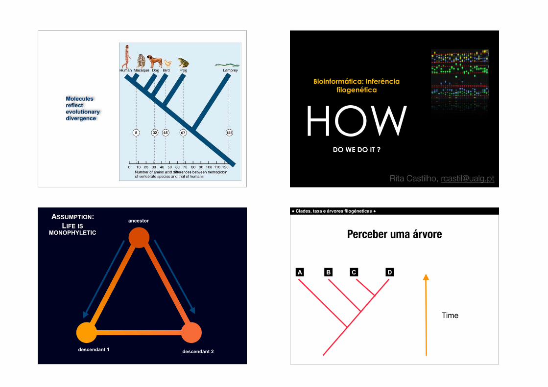
Molecules reflect evolutionary divergence
Bioinformática: Inferência filogenética
HOW DO WE DO IT ?
Rita Castilho, [email protected]
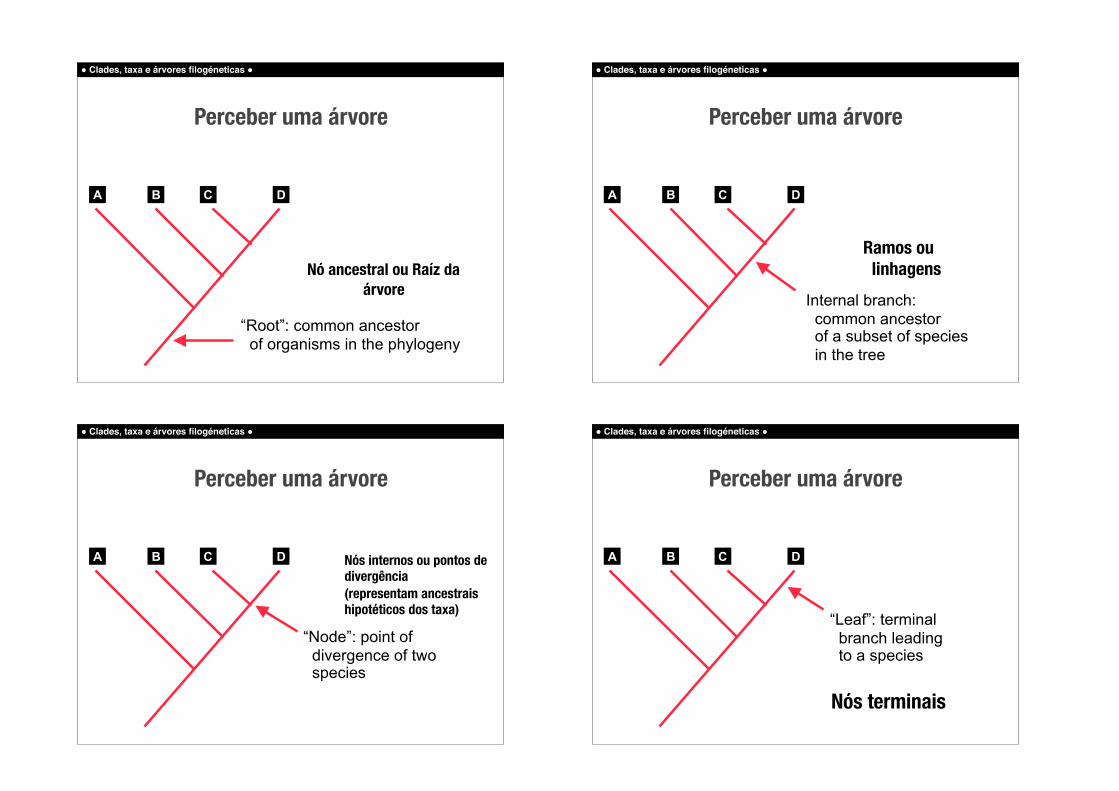
ancestor
descendant 1 descendant 2
ASSUMPTION: LIFE IS
MONOPHYLETIC
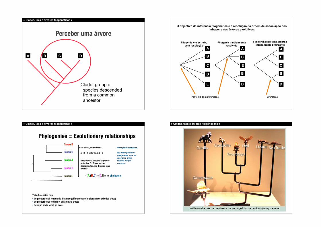
! Clades, taxa e árvores filogéneticas !
Time
Perceber uma árvore
B C DA
! Clades, taxa e árvores filogéneticas !
“Root”: common ancestor of organisms in the phylogeny
Perceber uma árvore
Nó ancestral ou Raíz da árvore
B C DA
! Clades, taxa e árvores filogéneticas !
Internal branch: common ancestor of a subset of species in the tree
Perceber uma árvore
Ramos ou linhagens
B C DA
! Clades, taxa e árvores filogéneticas !
“Node”: point of divergence of two species
Perceber uma árvore
Nós internos ou pontos de divergência (representam ancestrais hipotéticos dos taxa)
B C DA
! Clades, taxa e árvores filogéneticas !
“Leaf”: terminal branch leading to a species
Perceber uma árvore
Nós terminais
B C DA
! Clades, taxa e árvores filogéneticas !
Clade: group of species descended from a common ancestor
Perceber uma árvore
B C DA
Filogenia em estrela, sem resolução
Filogenia parcialmente resolvida
Filogenia resolvida, padrão inteiramente bifurcante
B
B
C
C
C
E
E
E
D
D D
Politomia or multifurcação Bifurcação
O objectivo da inferência filogenética é a resolução da ordem de associação das linhagens nas árvores evolutivas:
A A A
B
! Clades, taxa e árvores filogéneticas !
Phylogenies = Evolutionary relationships
((A,(B,C)),(D,E)) = phylogeny
B - C closer, sister clade A
Taxon A
Taxon B
Taxon C
Taxon E
Taxon D
This dimension can: • be proportional to genetic distance (diferences) = phylogram or adictive trees; • be proportional to time = ultrametric trees; • have no scale what so ever.
A - B - C, sister clade D - E
If there was a temporal or genetic scale then D - E taxa are the closest related, and diverged more recently
Alteração de caracteres.
Não tem significado o espaçamento entre os taxa nem a ordem absoluta porque aparecem.
! Clades, taxa e árvores filogéneticas !
! Clades, taxa e árvores filogéneticas !
All of these rearrangements show the same evolutionary relationships between
the taxaB
A
C
D
A
B
D
C
B
C
AD
B
D
AC
B
ACD
B
A
C
D
A
B
C
D
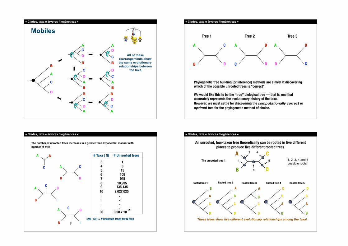
Mobiles ! Clades, taxa e árvores filogéneticas !
A C
B D
Tree 1
A B
C D
Tree 2
A B
D C
Tree 3
Phylogenetic tree building (or inference) methods are aimed at discovering which of the possible unrooted trees is "correct".
We would like this to be the “true” biological tree — that is, one that accurately represents the evolutionary history of the taxa. However, we must settle for discovering the computationally correct or optimal tree for the phylogenetic method of choice.
! Clades, taxa e árvores filogéneticas !
The number of unrooted trees increases in a greater than exponential manner with number of taxa
# Taxa ( N)
3 4 5 6 7 8 910 . . . .30
# Unrooted trees
1 3 15 105 945 10,935 135,135 2,027,025 . . . . 3.58 x 10
36
(2N - 5)!! = # unrooted trees for N taxa
CA
B D
A B
C
A D
B E
C
A D
B E
C
F
! Clades, taxa e árvores filogéneticas !
An unrooted, four-taxon tree theoretically can be rooted in five different places to produce five different rooted trees
The unrooted tree 1:
A C
B D
Rooted tree 4
C
D
A
B
4
Rooted tree 3
A
B
C
D
3
Rooted tree 5
D
C
A
B
5
Rooted tree 2
A
B
C
D
2
Rooted tree 1
B
A
C
D
1
These trees show five different evolutionary relationships among the taxa!
1, 2, 3, 4 and 5 possible roots
! Clades, taxa e árvores filogéneticas !
CA
B D
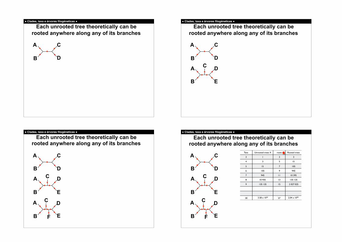
Each unrooted tree theoretically can be rooted anywhere along any of its branches
! Clades, taxa e árvores filogéneticas !
A D
B E
C
Each unrooted tree theoretically can be rooted anywhere along any of its branches
CA
B D
! Clades, taxa e árvores filogéneticas !
A D
B E
C
F
Each unrooted tree theoretically can be rooted anywhere along any of its branches
CA
B D
A D
B E
C
! Clades, taxa e árvores filogéneticas !
Each unrooted tree theoretically can be rooted anywhere along any of its branches
CA
B D
A D
B E
C
A D
B E
C
F
Taxa Unrooted trees X roots Rooted trees
3 1 3 3
4 3 5 15
5 15 7 105
6 105 9 945
7 945 11 10 395
8 10 935 13 135 125
9 135 135 15 2 027 025
30 3.58 x 1036 57 2.04 x 1038
! Clades, taxa e árvores filogéneticas !
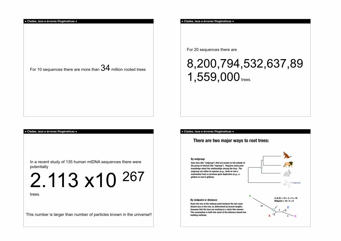
For 10 sequences there are more than 34 million rooted trees
! Clades, taxa e árvores filogéneticas !
For 20 sequences there are
8,200,794,532,637,891,559,000 trees.
! Clades, taxa e árvores filogéneticas !
In a recent study of 135 human mtDNA sequences there were potentially
2.113 x10 267 trees.
This number is larger than number of particles known in the universe!!
! Clades, taxa e árvores filogéneticas !
By outgroup: Uses taxa (the “outgroup”) that are known to fall outside of the group of interest (the “ingroup”). Requires some prior knowledge about the relationships among the taxa. The outgroup can either be species (e.g., birds to root a mammalian tree) or previous gene duplicates (e.g., a-globins to root b-globins).
There are two major ways to root trees:
A
B
C
D
10
2
3
5
2
By midpoint or distance: Roots the tree at the midway point between the two most distant taxa in the tree, as determined by branch lengths. Assumes that the taxa are evolving in a clock-like manner. This assumption is built into some of the distance-based tree building methods.
outgroup
d (A,D) = 10 + 3 + 5 = 18 Midpoint = 18 / 2 = 9
D
C
E
B
G H
F
J
I
K
A
Grouping 2
! Clades, taxa e árvores filogéneticas !
Grouping 1
D
C
E G
F
B
A
J
I
KH D
C
B
E G
F
H
A
J
I
K
Grouping 3
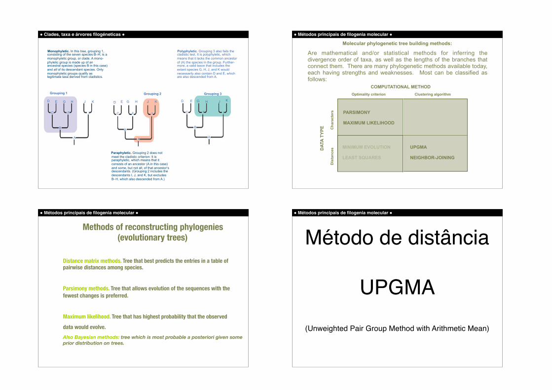
Monophyletic. In this tree, grouping 1, consisting of the seven species B–H, is a monophyletic group, or clade. A mono- phyletic group is made up of an ancestral species (species B in this case) and all of its descendant species. Only monophyletic groups qualify as legitimate taxa derived from cladistics.
Paraphyletic. Grouping 2 does not meet the cladistic criterion: It is paraphyletic, which means that it consists of an ancestor (A in this case) and some, but not all, of that ancestor’s descendants. (Grouping 2 includes the descendants I, J, and K, but excludes B–H, which also descended from A.)
Polyphyletic. Grouping 3 also fails the cladistic test. It is polyphyletic, which means that it lacks the common ancestor of (A) the species in the group. Further-more, a valid taxon that includes the extant species G, H, J, and K would necessarily also contain D and E, which are also descended from A.
! Métodos principais de filogenia molecular !
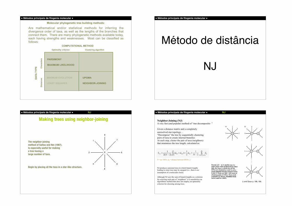
Molecular phylogenetic tree building methods:
Are mathematical and/or statistical methods for inferring the divergence order of taxa, as well as the lengths of the branches that connect them. There are many phylogenetic methods available today, each having strengths and weaknesses. Most can be classified as follows:
COMPUTATIONAL METHODClustering algorithmOptimality criterion
DAT
A TY
PE Cha
ract
ers
Dis
tanc
es
PARSIMONY
MAXIMUM LIKELIHOOD
UPGMA
NEIGHBOR-JOINING
MINIMUM EVOLUTION
LEAST SQUARES
! Métodos principais de filogenia molecular !
Methods of reconstructing phylogenies (evolutionary trees)
Distance matrix methods. Tree that best predicts the entries in a table of pairwise distances among species.
Parsimony methods. Tree that allows evolution of the sequences with the fewest changes is preferred.
Maximum likelihood. Tree that has highest probability that the observed
data would evolve. Also Bayesian methods: tree which is most probable a posteriori given some prior distribution on trees.
! Métodos principais de filogenia molecular !
Método de distância
UPGMA(Unweighted Pair Group Method with Arithmetic Mean)

! Métodos principais de filogenia molecular !
Seq sites1 T T A T T A A2 A A T T T A A3 A A A A A T A4 A A A A A A T
Distances
Distance-based methods: Transform the sequence data into pairwise distances (dissimilarities), and then use the matrix during tree building.
1 2 3 41 -2 3 -3 5 4 -4 5 4 2 -
! Métodos principais de filogenia molecular !
1 2 3 41 -2 3 -3 5 4 -4 5 4 2 -
! Métodos principais de filogenia molecular ! UPGMA
Construction of a distance tree using clustering with the Unweighted Pair Group Method with Arithmetic Mean (UPGMA)
From http://www.icp.ucl.ac.be/~opperd/private/upgma.html
A - GCTTGTCCGTTACGATB – ACTTGTCTGTTACGAT
First, construct a distance matrix:
A - GCTTGTCCGTTACGATB – ACTTGTCTGTTACGATC – ACCTGTCCGAAACGATD - ACTTGACCGTTTCCTTE – AGATGACCGTTTCGATF - ACTACACCCTTATGAG
A - GCTTGTCCGTTACGATC – ACCTGTCCGAAACGAT
A B C D E FA -B 2 -C 4 4 -D 6 6 6 -E 6 6 6 4F 8 8 8 8 8 -
! Métodos principais de filogenia molecular ! UPGMA
First round
dist(A,B),C = (distAC + distBC) / 2 = 4 dist(A,B),D = (distAD + distBD) / 2 = 6 dist(A,B),E = (distAE + distBE) / 2 = 6 dist(A,B),F = (distAF + distBF) / 2 = 8
Choose the most similar pair, cluster them together and calculate
the new distance matrix.
A B C D E FA -B 2 -C 4 4 -D 6 6 6 -E 6 6 6 4F 8 8 8 8 8 -
A,B C D E FA,B -C 4 -D 6 6 -E 6 6 4F 8 8 8 8 -
! Métodos principais de filogenia molecular ! UPGMA
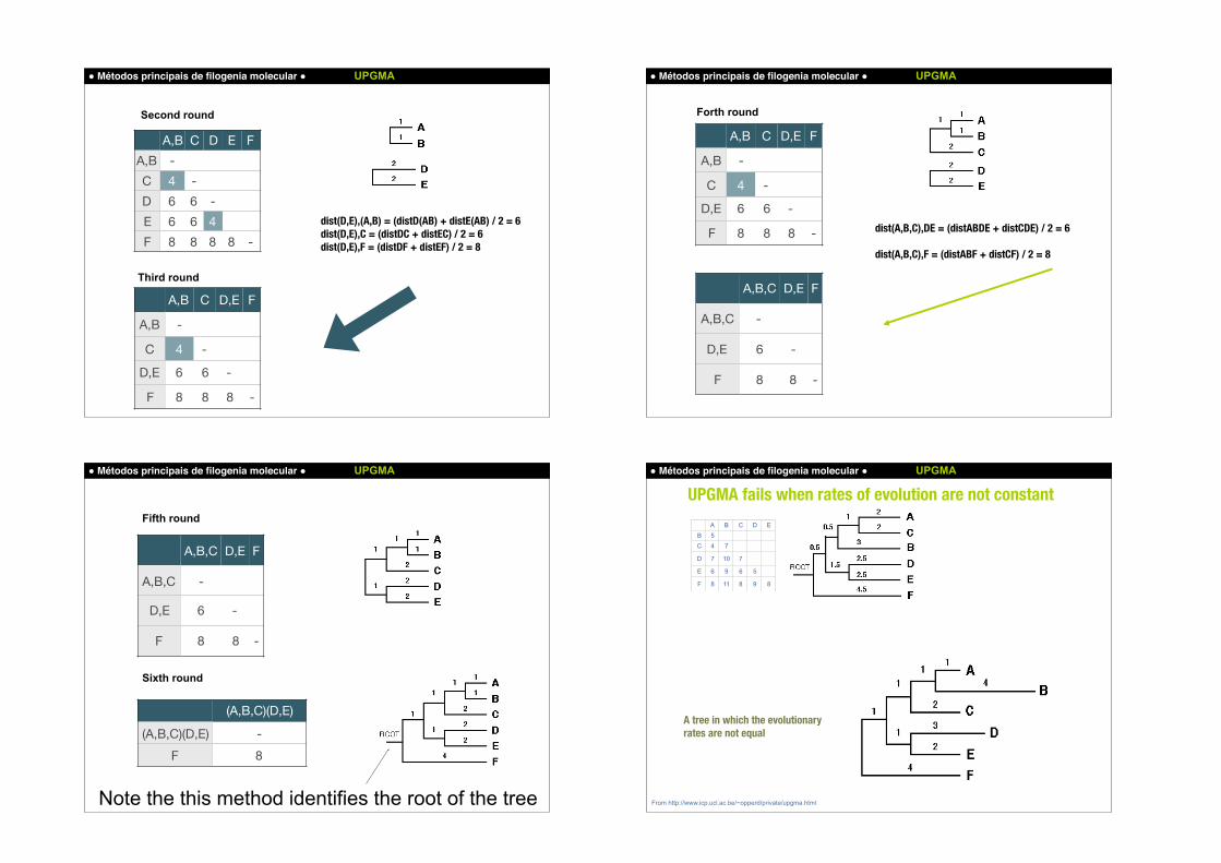
Second round
Third round
dist(D,E),(A,B) = (distD(AB) + distE(AB) / 2 = 6 dist(D,E),C = (distDC + distEC) / 2 = 6 dist(D,E),F = (distDF + distEF) / 2 = 8
A,B C D E FA,B -C 4 -D 6 6 -E 6 6 4F 8 8 8 8 -
A,B C D,E F
A,B -
C 4 -
D,E 6 6 -
F 8 8 8 -
! Métodos principais de filogenia molecular ! UPGMA
Forth round
dist(A,B,C),DE = (distABDE + distCDE) / 2 = 6 dist(A,B,C),F = (distABF + distCF) / 2 = 8
A,B C D,E F
A,B -
C 4 -
D,E 6 6 -
F 8 8 8 -
A,B,C D,E F
A,B,C -
D,E 6 -
F 8 8 -
! Métodos principais de filogenia molecular ! UPGMA
Fifth round
Sixth round
Note the this method identifies the root of the tree
A,B,C D,E F
A,B,C -
D,E 6 -
F 8 8 -
(A,B,C)(D,E)
(A,B,C)(D,E) -F 8
! Métodos principais de filogenia molecular ! UPGMA
UPGMA fails when rates of evolution are not constant
A tree in which the evolutionary rates are not equal
From http://www.icp.ucl.ac.be/~opperd/private/upgma.html
A B C D E B 5 C 4 7
D 7 10 7
E 6 9 6 5
F 8 11 8 9 8
! Métodos principais de filogenia molecular !
Molecular phylogenetic tree building methods:
Are mathematical and/or statistical methods for inferring the divergence order of taxa, as well as the lengths of the branches that connect them. There are many phylogenetic methods available today, each having strengths and weaknesses. Most can be classified as follows:
COMPUTATIONAL METHODClustering algorithmOptimality criterion
DAT
A TY
PE Cha
ract
ers
Dis
tanc
es
PARSIMONY
MAXIMUM LIKELIHOOD
UPGMA
NEIGHBOR-JOINING
MINIMUM EVOLUTION
LEAST SQUARES
! Métodos principais de filogenia molecular !
Método de distância
NJ
! Métodos principais de filogenia molecular ! NJ
The neighbor-joining method of Saitou and Nei (1987). Is especially useful for making a tree having a large number of taxa.
Begin by placing all the taxa in a star-like structure.
Making trees using neighbor-joining ! Métodos principais de filogenia molecular ! NJ
Neighbor-Joining (NJ) A very fast (and popular) method of “star decomposition”
Given a distance matrix and a completely unresolved star topology… “Decompose” the tree by sequentially clustering pairs of taxa to create internal branches At each step, cluster the pair of taxa (neighbors) that minimizes the tree length, calculated as:
N = no. OTUs, dij = distance between OTUS i, j
NJ produces unrooted trees in which branch lengths leading to sister taxa may be unequal (i.e., there is no assumption of a molecular clock).
Although NJ uses the sum of branch lengths as a criterion for selecting each pair of “neighbors” it is nonetheless an algorithmic method that does not employ an optimality criterion for choosing among trees.
Li and Graur p. 188, 189.

! Métodos principais de filogenia molecular ! NJ
Tree-building methods: Neighbor-joining
Next, identify neighbors (e.g. 1 and 2) that are most closely related. Connect these neighbors to other OTUs via an internal branch, XY. At each successive stage, minimize the sum of the branch lengths.
! Métodos principais de filogenia molecular ! NJ
Tree-building methods: Neighbor joining
Define the distance from X to Y by
dXY = 1/2(d1Y + d2Y – d12)
! Métodos principais de filogenia molecular ! NJ
The neighbor joining method joins at each step, the two closest sub-trees that are not already joined. It is based on the minimum evolution principle. One of the important concepts in the NJ method is neighbors, which are defined as two taxa that are connected by a single node in an unrooted tree
A B
Node 1
! Métodos principais de filogenia molecular ! NJ
A
B
C
D
E
A
B
5
C
4
7
D
7
10
7
E
6
9
6
5
F 8 11 8 9 8
B
C
D
E
F
A
! Métodos principais de filogenia molecular ! NJ
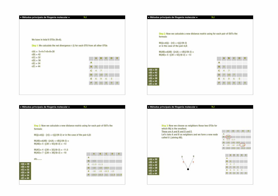
We have in total 6 OTUs (N=6).
Step 1: We calculate the net divergence r (i) for each OTU from all other OTUs
r(A) = 5+4+7+6+8=30 r(B) = 42 r(C) = 32 r(D) = 38 r(E) = 34 r(F) = 44
A
B
C
D
E
A
B
5
C
4
7
D
7
10
7
E
6
9
6
5
F 8 11 8 9 8
! Métodos principais de filogenia molecular ! NJ
Step 2: Now we calculate a new distance matrix using for each pair of OUTs the formula:
M(ij)=d(ij) - [r(i) + r(j)]/(N-2) or in the case of the pair A,B:
M(AB)=d(AB) -[(r(A) + r(B)]/(N-2) = M(AB)= 5 -[(30 + 42]/(6-2) = -13
A
B
C
D
E
A
B
5
C
4
7
D
7
10
7
E
6
9
6
5
F 8 11 8 9 8
r(A) = 30r(B) = 42r(C) = 32r(D) = 38r(E) = 34r(F) = 44
! Métodos principais de filogenia molecular ! NJ
Step 2: Now we calculate a new distance matrix using for each pair of OUTs the formula:
M(ij)=d(ij) - [r(i) + r(j)]/(N-2) or in the case of the pair A,B:
M(AB)=d(AB) -[(r(A) + r(B)]/(N-2) = M(AB)= 5 -[(30 + 42]/(6-2) = -13
M(AC)= 4 -[(30 + 32]/(6-2) = -11.5 M(AD)= 7 -[(30 + 38]/(6-2) = -10
etc........
A
B
C
D
E
A
B
-13
C
-11.5
-11.5
D
-10
-10
-10.5
E
-10
-10
-10.5
-13
F -10.5 -10.5 11 -11.5 -11.5
r(A) = 30r(B) = 42r(C) = 32r(D) = 38r(E) = 34r(F) = 44
! Métodos principais de filogenia molecular ! NJ
Step 3: Now we choose as neighbors those two OTUs for which Mij is the smallest. These are A and B and D and E. Let's take A and B as neighbors and we form a new node called U ( joining AB).
A
B
C
D
E
A
B
-13
C
-11.5
-11.5
D
-10
-10
-10.5
E
-10
-10
-10.5
-13
F -10.5 -10.5 11 -11.5 -11.5
A
B
C
D
E
A
B
5
C
4
7
D
7
10
7
E
6
9
6
5
F 8 11 8 9 8
r(A) = 30r(B) = 42r(C) = 32r(D) = 38r(E) = 34r(F) = 44
BA
? ?
! Métodos principais de filogenia molecular ! NJ
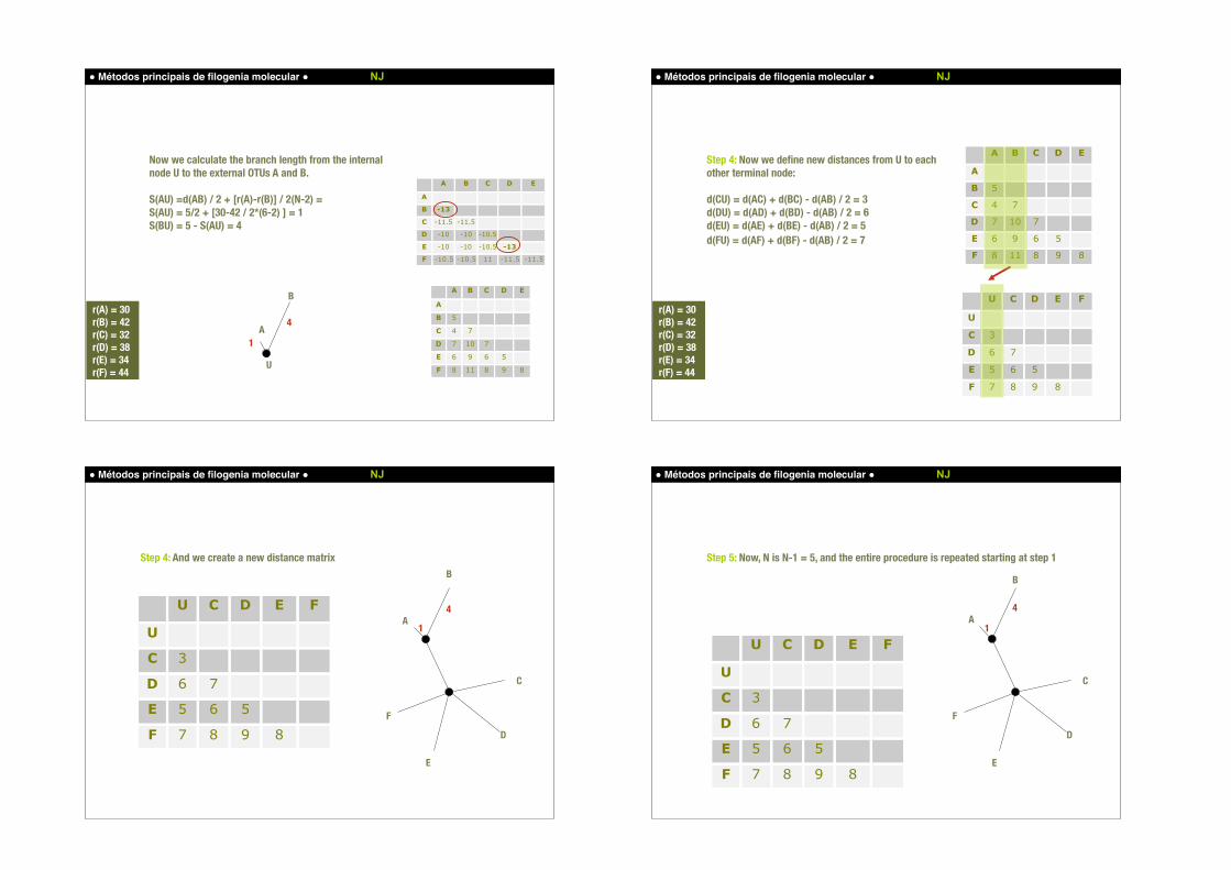
Now we calculate the branch length from the internal node U to the external OTUs A and B.
S(AU) =d(AB) / 2 + [r(A)-r(B)] / 2(N-2) = S(AU) = 5/2 + [30-42 / 2*(6-2) ] = 1 S(BU) = 5 - S(AU) = 4
A
B
C
D
E
A
B
-13
C
-11.5
-11.5
D
-10
-10
-10.5
E
-10
-10
-10.5
-13
F -10.5 -10.5 11 -11.5 -11.5
A
B
C
D
E
A
B
5
C
4
7
D
7
10
7
E
6
9
6
5
F 8 11 8 9 8
r(A) = 30r(B) = 42r(C) = 32r(D) = 38r(E) = 34r(F) = 44
B
A1
4
U
! Métodos principais de filogenia molecular ! NJ
Step 4: Now we define new distances from U to each other terminal node:
d(CU) = d(AC) + d(BC) - d(AB) / 2 = 3 d(DU) = d(AD) + d(BD) - d(AB) / 2 = 6 d(EU) = d(AE) + d(BE) - d(AB) / 2 = 5 d(FU) = d(AF) + d(BF) - d(AB) / 2 = 7
A
B
C
D
E
A
B
5
C
4
7
D
7
10
7
E
6
9
6
5
F 8 11 8 9 8
U
C
D
E
F
U
C
3
D
6
7
E
5
6
5
F
7
8
9
8
r(A) = 30r(B) = 42r(C) = 32r(D) = 38r(E) = 34r(F) = 44
! Métodos principais de filogenia molecular ! NJ
Step 4: And we create a new distance matrix
U
C
D
E
F
U
C
3
D
6
7
E
5
6
5
F
7
8
9
8
B
C
D
E
F
A 1
4
! Métodos principais de filogenia molecular ! NJ
Step 5: Now, N is N-1 = 5, and the entire procedure is repeated starting at step 1
U
C
D
E
F
U
C
3
D
6
7
E
5
6
5
F
7
8
9
8
B
C
D
E
F
A1
4
! Métodos principais de filogenia molecular ! NJ
B
C
D
E
F
A
1
1
0.5
4
21
4.752.25
2.75
! Métodos principais de filogenia molecular !
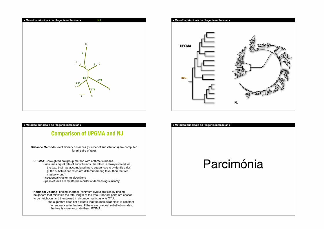
UPGMA
NJ
ROOT
! Métodos principais de filogenia molecular !
Comparison of UPGMA and NJ
Neighbor Joining: finding shortest (minimum evolution) tree by finding neighbors that minimize the total length of the tree. Shortest pairs are chosen to be neighbors and then joined in distance matrix as one OTU.
- the algorithm does not assume that the molecular clock is constant for sequences in the tree. If there are unequal substitution rates, the tree is more accurate than UPGMA.
Distance Methods: evolutionary distances (number of substitutions) are computed for all pairs of taxa.
UPGMA: unweighted pairgroup method with arithmetic means. - assumes equal rate of substitutions (therefore is always rooted, as
the taxa that has accumulated more sequences is evidently older) (if the substitutions rates are different among taxa, then the tree maybe wrong)
- sequential clustering algorithms - pairs of taxa are clustered in order of decreasing similarity
! Métodos principais de filogenia molecular !
Parcimónia
! Métodos principais de filogenia molecular !
Molecular phylogenetic tree building methods:
Are mathematical and/or statistical methods for inferring the divergence order of taxa, as well as the lengths of the branches that connect them. There are many phylogenetic methods available today, each having strengths and weaknesses. Most can be classified as follows:
COMPUTATIONAL METHODClustering algorithmOptimality criterion
DAT
A TY
PE Cha
ract
ers
Dis
tanc
es
PARSIMONY
MAXIMUM LIKELIHOOD
UPGMA
NEIGHBOR-JOINING
MINIMUM EVOLUTION
LEAST SQUARES
! Métodos principais de filogenia molecular ! Maximum parsimony
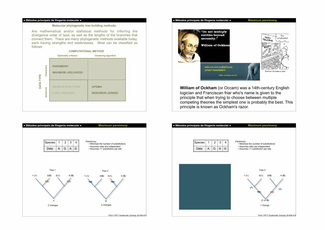
William of Ockham (or Occam) was a 14th-century English logician and Franciscan friar who's name is given to the principle that when trying to choose between multiple competing theories the simplest one is probably the best. This principle is known as Ockham's razor.
! Métodos principais de filogenia molecular ! Maximum parsimony
Parsimony: • Minimize the number of substitutions • Assumes sites are independent • Assumes <1 substitution per site
Tree 1
1 (A) 2(G) 3(A) 4 (G)
2 changes
A
Species 1 2 3 4
Data A G A G
Tree 2
1 (A) 2(G) 3(A) 4 (G)
G
2 changes
Fitch (1971) Systematic Zoology 20:406-416
! Métodos principais de filogenia molecular ! Maximum parsimony
Parsimony: • Minimize the number of substitutions • Assumes sites are independent • Assumes <1 substitution per site
Tree 1 and 2 Tree 3
1 (A) 2(G) 3(A) 4 (G)
(A or G) (A or G)
2 changes
(A or G)
1 (A) 2(G)3(A) 4 (G)
(A)(G)
(A or G)
1 change
Species 1 2 3 4
Data A G A G
Fitch (1971) Systematic Zoology 20:406-416
! Métodos principais de filogenia molecular ! Maximum parsimony
Parsimony: • Minimize the number of substitutions • Assumes sites are independent • Assumes <1 substitution per site
Tree 1 Tree 2
1 (A) 2(G) 3(A) 4 (G)
(A or G) (A or G)
2 changes
(A or G)
1 (A) 2(G)3(A) 4 (G)
(A) (G)
(A or G)
1 change
More parsimonious
Fitch (1971) Systematic Zoology 20:406-416
Species 1 2 3 4
Data A G A G
! Métodos principais de filogenia molecular ! Maximum parsimony
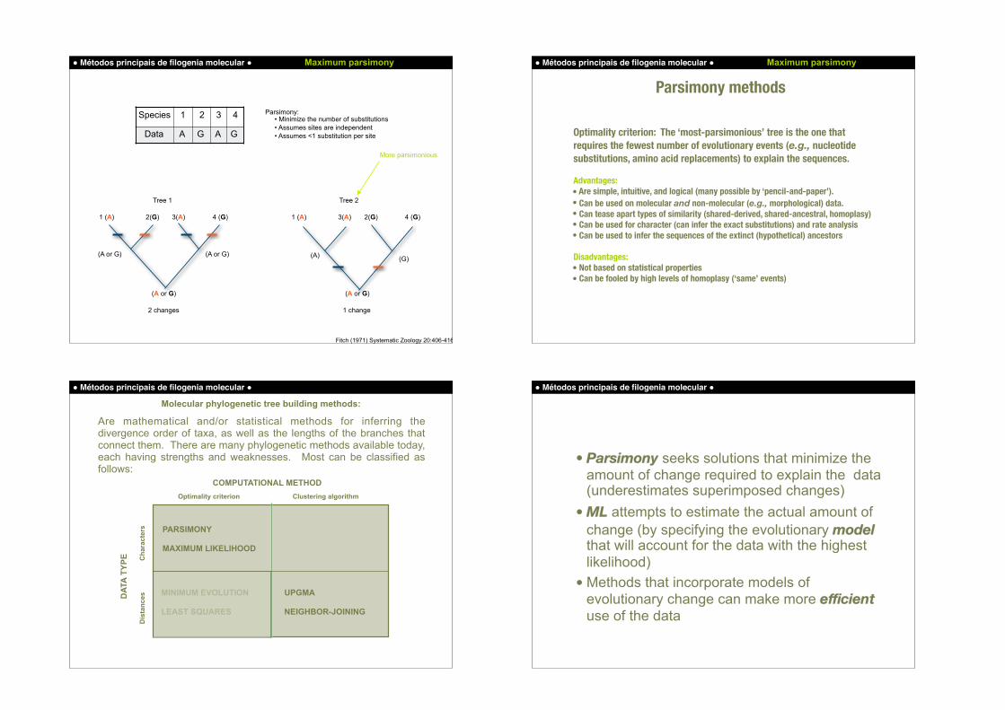
Parsimony methods
Optimality criterion: The ‘most-parsimonious’ tree is the one that requires the fewest number of evolutionary events (e.g., nucleotide substitutions, amino acid replacements) to explain the sequences.
Advantages: • Are simple, intuitive, and logical (many possible by ‘pencil-and-paper’). • Can be used on molecular and non-molecular (e.g., morphological) data. • Can tease apart types of similarity (shared-derived, shared-ancestral, homoplasy) • Can be used for character (can infer the exact substitutions) and rate analysis • Can be used to infer the sequences of the extinct (hypothetical) ancestors
Disadvantages: • Not based on statistical properties • Can be fooled by high levels of homoplasy (‘same’ events)
! Métodos principais de filogenia molecular !
Molecular phylogenetic tree building methods:
Are mathematical and/or statistical methods for inferring the divergence order of taxa, as well as the lengths of the branches that connect them. There are many phylogenetic methods available today, each having strengths and weaknesses. Most can be classified as follows:
COMPUTATIONAL METHODClustering algorithmOptimality criterion
DAT
A TY
PE Cha
ract
ers
Dis
tanc
es
PARSIMONY
MAXIMUM LIKELIHOOD
UPGMA
NEIGHBOR-JOINING
MINIMUM EVOLUTION
LEAST SQUARES
! Métodos principais de filogenia molecular !
• Parsimony seeks solutions that minimize the amount of change required to explain the data (underestimates superimposed changes)
• ML attempts to estimate the actual amount of change (by specifying the evolutionary model that will account for the data with the highest likelihood)
• Methods that incorporate models of evolutionary change can make more efficient use of the data
! Métodos principais de filogenia molecular ! Maximum likelihood
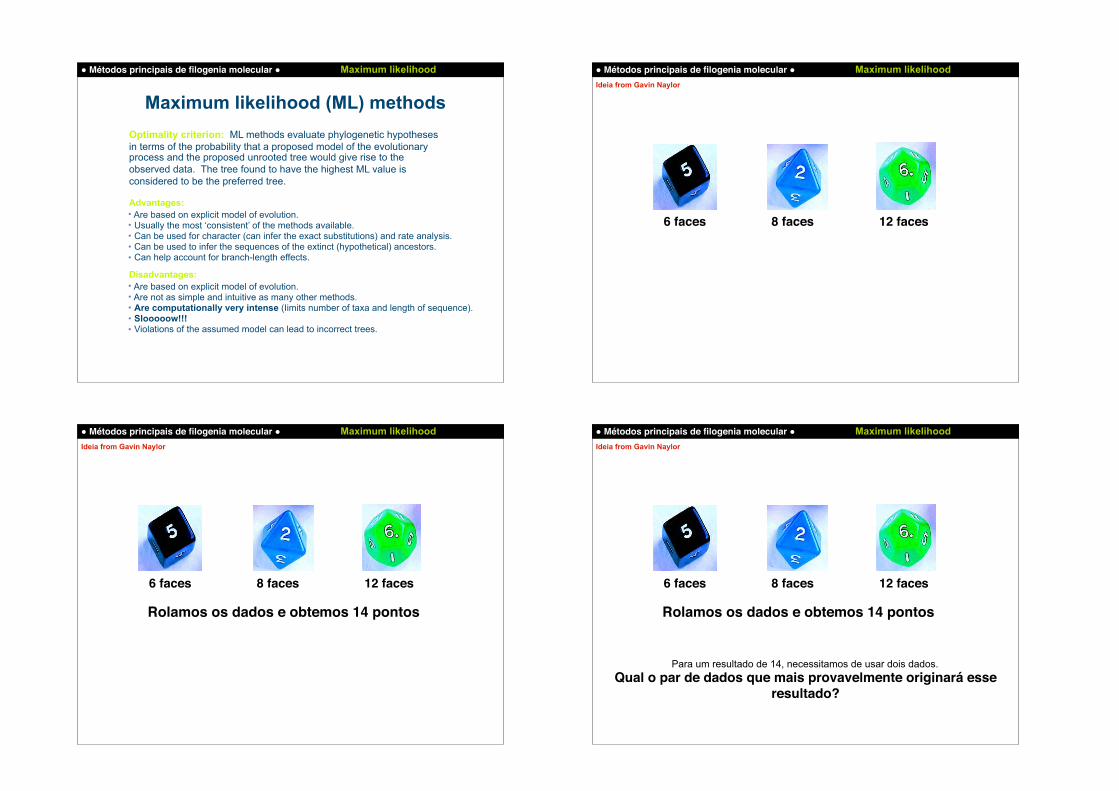
Maximum likelihood (ML) methodsOptimality criterion: ML methods evaluate phylogenetic hypotheses in terms of the probability that a proposed model of the evolutionary process and the proposed unrooted tree would give rise to the observed data. The tree found to have the highest ML value is considered to be the preferred tree.
Advantages: • Are based on explicit model of evolution. • Usually the most ‘consistent’ of the methods available. • Can be used for character (can infer the exact substitutions) and rate analysis. • Can be used to infer the sequences of the extinct (hypothetical) ancestors. • Can help account for branch-length effects.
Disadvantages: • Are based on explicit model of evolution. • Are not as simple and intuitive as many other methods. • Are computationally very intense (Iimits number of taxa and length of sequence). • Slooooow!!! • Violations of the assumed model can lead to incorrect trees.
! Métodos principais de filogenia molecular ! Maximum likelihood
6 faces 8 faces 12 faces
Ideia from Gavin Naylor
! Métodos principais de filogenia molecular ! Maximum likelihood
Rolamos os dados e obtemos 14 pontos
Ideia from Gavin Naylor
6 faces 8 faces 12 faces
! Métodos principais de filogenia molecular ! Maximum likelihood
Para um resultado de 14, necessitamos de usar dois dados. Qual o par de dados que mais provavelmente originará esse
resultado?
Rolamos os dados e obtemos 14 pontos
Ideia from Gavin Naylor
6 faces 8 faces 12 faces
! Métodos principais de filogenia molecular ! Maximum likelihood
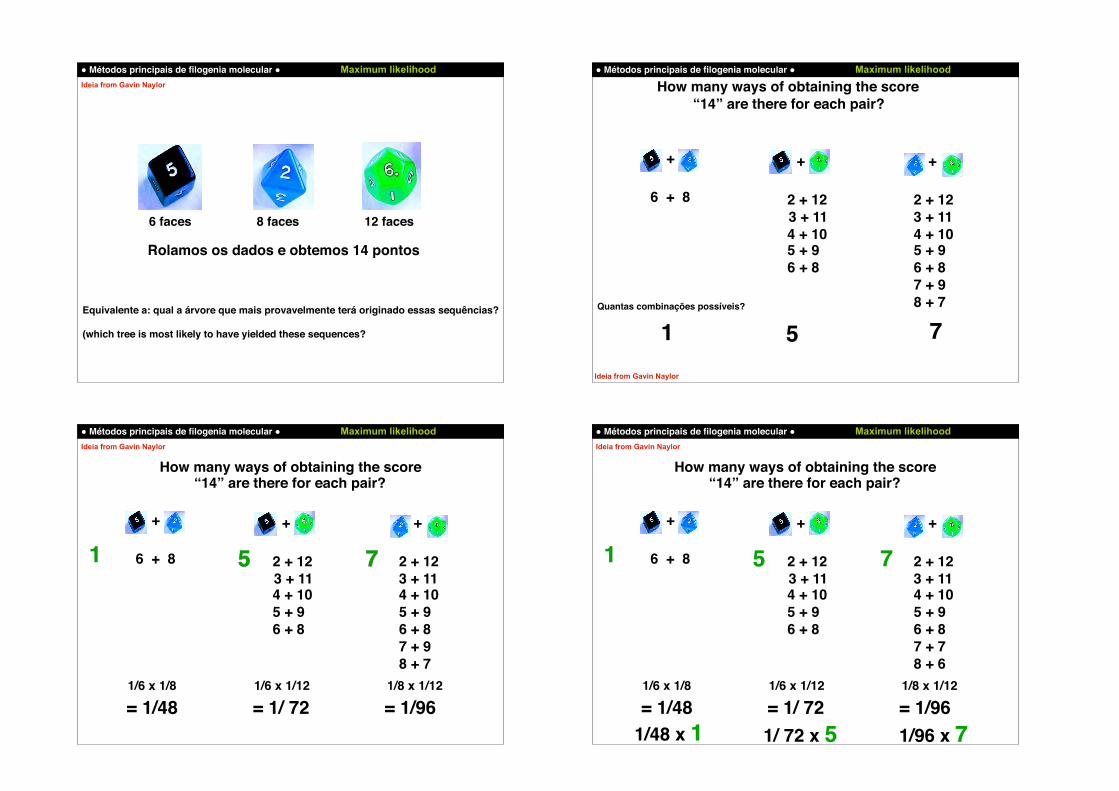
Equivalente a: qual a árvore que mais provavelmente terá originado essas sequências?
(which tree is most likely to have yielded these sequences?
Rolamos os dados e obtemos 14 pontos
Ideia from Gavin Naylor
6 faces 8 faces 12 faces
! Métodos principais de filogenia molecular ! Maximum likelihood
6 + 8
+ + +
How many ways of obtaining the score “14” are there for each pair?
2 + 12 3 + 11 4 + 10
5 + 96 + 8
1 5 7Ideia from Gavin Naylor
Quantas combinações possíveis?
2 + 12 3 + 11 4 + 10
5 + 96 + 87 + 98 + 7
! Métodos principais de filogenia molecular ! Maximum likelihood
6 + 8
+ + +
How many ways of obtaining the score “14” are there for each pair?
2 + 12 3 + 11 4 + 10
5 + 96 + 8
1 5 7
Ideia from Gavin Naylor
2 + 12 3 + 11 4 + 10
5 + 96 + 87 + 98 + 7
1/6 x 1/8
= 1/481/6 x 1/12 1/8 x 1/12
= 1/ 72 = 1/96
5 7
! Métodos principais de filogenia molecular ! Maximum likelihood
6 + 8
+ + +
How many ways of obtaining the score “14” are there for each pair?
2 + 12 3 + 11 4 + 10
5 + 96 + 8
1 5 7
Ideia from Gavin Naylor
2 + 12 3 + 11 4 + 10
5 + 96 + 87 + 78 + 6
1/6 x 1/8
= 1/481/6 x 1/12 1/8 x 1/12
= 1/ 72 = 1/961/48 x 1 1/ 72 x 5 1/96 x 7
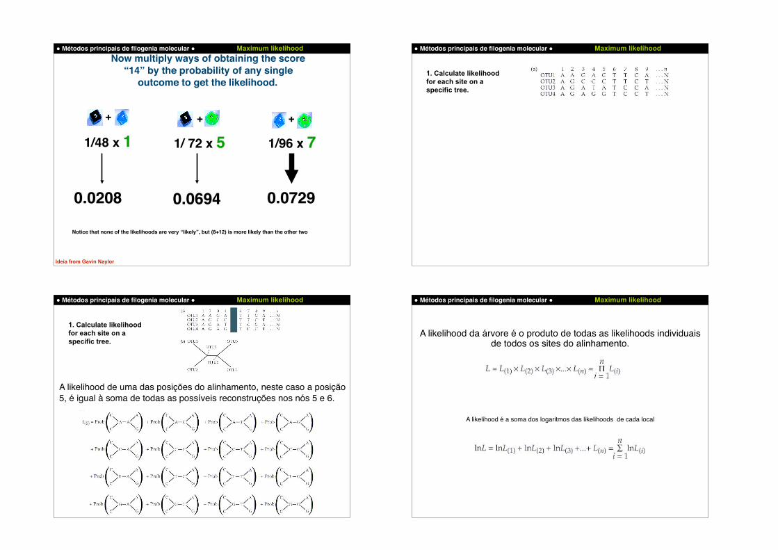
! Métodos principais de filogenia molecular ! Maximum likelihoodNow multiply ways of obtaining the score
“14” by the probability of any single outcome to get the likelihood.
+ + +
1/48 x 1 1/ 72 x 5 1/96 x 7
0.07290.06940.0208
Notice that none of the likelihoods are very “likely”, but (8+12) is more likely than the other two
Ideia from Gavin Naylor
! Métodos principais de filogenia molecular ! Maximum likelihood
1. Calculate likelihood for each site on a specific tree.
! Métodos principais de filogenia molecular ! Maximum likelihood
1. Calculate likelihood for each site on a specific tree.
A likelihood de uma das posições do alinhamento, neste caso a posição 5, é igual à soma de todas as possíveis reconstruções nos nós 5 e 6.
! Métodos principais de filogenia molecular ! Maximum likelihood
A likelihood da árvore é o produto de todas as likelihoods individuais de todos os sites do alinhamento.
A likelihood é a soma dos logaritmos das likelihoods de cada local