Biogeographic dating of speciation times using ... · 22 stochastic process may be used to estimate absolute ... I analyze the well-studied turtle ... 92 nario as a calibration point

Biogeographic dating of speciation times using1

paleogeographically informed processes2

R.H. Biogeographic dating of speciation times3

Michael J. Landis 14

1Department of Integrative Biology5

University of California, Berkeley, CA 94720-3140, U.S.A.6

Michael J. Landis7

University of California, Berkeley8

Department of Integrative Biology9

3060 VLSB #314010

Berkeley, CA 94720-314011

U.S.A.12

Phone: (510) 642-123313

E-mail: [email protected]

.CC-BY 4.0 International licensepeer-reviewed) is the author/funder. It is made available under aThe copyright holder for this preprint (which was not. http://dx.doi.org/10.1101/028738doi: bioRxiv preprint first posted online Oct. 8, 2015;

http://dx.doi.org/10.1101/028738

http://creativecommons.org/licenses/by/4.0/

Abstract15

Standard models of molecular evolution cannot estimate absolute speciation times alone,16

and require external calibrations to do so. Because fossil calibration methods rely on the17

unreliable fossil record, most nodes in the tree of life are dated with poor accuracy. However,18

many major paleogeographical events are dated, and since biogeographic processes depend19

on paleogeographical conditions, biogeographic dating may be used as an alternative or20

complementary method to fossil dating. I demonstrate how a time-stratified biogeographic21

stochastic process may be used to estimate absolute divergence times by conditioning on22

dated paleogeographical events. Informed by the current paleogeographical literature, I23

construct an empirical dispersal graph using 25 areas and 26 epochs for the past 540 Ma24

of Earth’s history. Simulations indicate biogeographic dating performs well so long as pa-25

leogeography imposes constraint on biogeographic character evolution. To gauge whether26

biogeographic dating may have any practical use, I analyze the well-studied turtle clade (Tes-27

tudines) then assess how well biogeographic dating fares compared to heavily fossil-calibrated28

dating results as reported in the literature. Fossil-free biogeographic dating estimated the29

age of the most recent common ancestor of extant turtles to be approximately 201 Ma, which30

is consistent with fossil-based estimates. Accuracy improves further when including a root31

node fossil calibration. The described model, paleogeographical dispersal graph, and analysis32

scripts are available for use with RevBayes.33

1 Introduction34

Time is a simple and fundamental axis of evolution. Knowing the order and timing of35

evolutionary events grants us insight into how vying evolutionary processes interact. With36

a perfectly accurate catalog of geologically-dated speciation times, many macroevolutionary37

questions would yield to simple interrogation, such as whether one clade exploded with38

diversity before or after a niche-analogous clade went extinct, or whether some number of39

contemporaneous biota were eradicated simultaneously by the same mass extinction event.40

1


http://dx.doi.org/10.1101/028738


Only rarely does the fossil record give audience to the exact history of evolutionary events:41

it is infamously irregular across time, space, and species, so biologists generally resort to42

inference to estimate when, where, and what happened to fill those gaps. That said, we have43

not yet found a perfect character or model to infer dates for divergence times, so advances44

in dating strategies are urgently needed. A brief survey of the field reveals why.45

The molecular clock hypothesis of Zuckerkandl and Pauling (1962) states that if substi-46

tutions arise (i.e. alleles fix) at a constant rate, the expected number of substitutions is the47

product of the substitution rate and the time the substitution process has been operating.48

With data from extant taxa, we only observe the outcome of the evolutionary process for an49

unknown rate and an unknown amount of time. As such, rate and time are non-identifiable50

under standard models of molecular substitution, so inferred amounts of evolutionary change51

are often reported as a compound parameter, the product of rate and time, called length.52

If all species’ shared the same substitution rate, a phylogeny with branches measured in53

lengths would give relative divergence times, i.e. proportional to absolute divergence times.54

While it is reasonable to say species’ evolution shares a basis in time, substitution rates55

differ between species and over macroevolutionary timescales (Wolfe et al. 1987; Martin and56

Palumbi 1993). Even when imposing a model of rate heterogeneity (Thorne et al. 1998;57

Drummond et al. 2006), only relative times may be estimated. Extrinsic information, i.e. a58

dated calibration point, is needed to establish an absolute time scaling, and typically takes59

form as a fossil occurrence or paleogeographical event.60

When fossils are available, they currently provide the most accurate inroad to calibrate61

divergence events to geological timescales, largely because each fossil is associated with a62

geological occurrence time. Fossil ages may be used in several ways to calibrate divergence63

times. The simplest method is the fossil node calibration, whereby the fossil is associated64

with a clade and constrains its time of origin (Ho and Phillips 2009; Parham et al. 2011).65

Node calibrations are empirical priors, not data-dependent stochastic processes, so they de-66

pend entirely on experts’ abilities to quantify the distribution of plausible ages for the given67

node. That is, node calibrations do not arise from a generative evolutionary process. Since68

2


http://dx.doi.org/10.1101/028738


molecular phylogenies cannot identify rate from time, then the time scaling is entirely deter-69

mined by the prior, i.e. the posterior is perfectly prior-sensitive for rates and times. Rather70

than using prior node calibrations, fossil tip dating (Pyron 2011; Ronquist et al. 2012) treats71

fossil occurrences as terminal taxa with morphological characters as part of any standard72

phylogenetic analysis. In this case, the model of character evolution, tree prior, and fossil73

ages generate the distribution of clade ages, relying on the fossil ages and a morphological74

clock to induce time calibrations. To provide a generative process of fossilization, Heath et al.75

(2014) introduced the fossilized birth-death process, by which lineages speciate, go extinct,76

or produce fossil observations. Using fossil tip dating with the fossilized birth-death process,77

Gavryushkina et al. (2015) demonstrated multiple calibration techniques may be used jointly78

in a theoretically consistent framework (i.e. without introducing model violation).79

Of course, fossil calibrations require fossils, but many clades leave few to no known fos-80

sils due to taphonomic processes, which filter out species with too soft or too fragile of81

tissues, or with tissues that were buried in substrates that were too humid, too arid, or82

too rocky; or due to sampling biases, such as geographical or political biases imbalancing83

collection efforts (Behrensmeyer et al. 2000; Kidwell and Holland 2002). Although these84

biases do not prohibitively obscure the record for widespread species with robust mineral-85

ized skeletons—namely, large vertebrates and marine invertebrates—fossil-free calibration86

methods are desperately needed to date the remaining majority of nodes in the tree of life.87

In this direction, analogous to fossil node dating, node dates may be calibrated using pa-88

leobiogeographic scenarios (Heads 2005; Renner 2005). For example, an ornithologist might89

reasonably argue that a bird known as endemic to a young island may have speciated only90

after the island was created, thus providing a maximum age of origination. Using this sce-91

nario as a calibration point excludes the possibility of alternative historical biogeographic92

explanations, e.g. the bird might have speciated off-island before the island surfaced and93

migrated there afterwards. See Heads (2005; 2011), Kodandaramaiah (2011), and Ho et al.94

(2015) for discussion on the uses and pitfalls of biogeographic node calibrations. Like fossil95

node calibrations, biogeographic node calibrations fundamentally rely on some prior distri-96

3


http://dx.doi.org/10.1101/028738


bution of divergence times, opinions may vary from expert to expert, making results difficult97

to compare from a modeling perspective. Worsening matters, the time and context of bio-98

geographic events are never directly observed, so asserting that a particular dispersal event99

into an island system resulted in a speciation event to calibrate a node fails to account for100

the uncertainty that the assumed evolutionary scenario took place at all. Ideally, all possible101

biogeographic and diversification scenarios would be considered, with each scenario given102

credence in proportion to its probability.103

Inspired by advents in fossil dating models (Pyron 2011; Ronquist et al. 2012; Heath104

et al. 2014), which have matured from phenomenological towards mechanistic approaches105

(Rodrigue and Philippe 2010), I present an explicitly data-dependent and process-based106

biogeographic method for divergence time dating to formalize the intuition underlying bio-107

geographic node calibrations. Analogous to fossil tip dating, the goal is to allow the observed108

biogeographic states at the “tips” of the tree induce a posterior distribution of dated specia-109

tion times by way of an evolutionary process. By modeling dispersal rates between areas as110

subject to time-calibrated paleogeographical information, such as the merging and splitting111

of continental adjacencies due to tectonic drift, particular dispersal events between area-112

pairs are expected to occur with higher probability during certain geological time intervals113

than during others. For example, the dispersal rate between South America and Africa was114

likely higher when they were joined as West Gondwana (ca 120 Ma) than when separated as115

they are today. If the absolute timing of dispersal events on a phylogeny matters, then so116

must the absolute timing of divergence events. Unlike fossil tip dating, biogeographic dating117

should, in principle, be able to date speciation times only using extant taxa.118

To illustrate how this is possible, I construct a toy biogeographic example to demonstrate119

when paleogeography may date divergence times, then follow with a more formal descrip-120

tion of the model. By performing joint inference with molecular and biogeographic data, I121

demonstrate the effectiveness of biogeographic dating by applying it to simulated and empir-122

ical scenarios, showing rate and time are identifiable. While researchers have accounted for123

phylogenetic uncertainty in biogeographic analyses (Nylander et al. 2008; Lemey et al. 2009;124

4


http://dx.doi.org/10.1101/028738


Beaulieu et al. 2013), I am unaware of work demonstrating how paleogeographic calibrations125

may be leveraged to date divergence times via a biogeographic process. For the empirical126

analysis, I date the divergence times for Testudines using biogeographic dating, first without127

any fossils, then using a fossil root node calibration. Finally, I discuss the strengths and128

weaknesses of my method, and how it may be improved in future work.129

2 Model130

2.1 The anatomy of biogeographic dating131

Briefly, I will introduce an example of how time-calibrated paleogeographical events may132

impart information through a biogeographic process to date speciation times, then later133

develop the details underlying the strategy, which I call biogeographic dating. Throughout134

the manuscript, I assume a rooted phylogeny, Ψ, with known topology but with unknown135

divergence times that I wish to estimate. Time is measured in geological units and as136

time until present, with t = 0 being the present, t < 0 being the past, and age being the137

negative amount of time until present. To keep the model of biogeographic evolution simple,138

the observed taxon occurrence matrix, Z, is assumed to be generated by a discrete-valued139

dispersal process where each taxon is present in only a single area at a time (Sanmartın et al.140

2008). For example, taxon T1 might be coded to be found in Area A or Area B but not both141

simultaneously. Although basic, this model is sufficient to make use of paleogeographical142

information, suggesting more realistic models will fare better.143

Consider two areas, A and B, that drift into and out of contact over time. When in144

contact, dispersal is possible; when not, impossible. Represented as a graph, A and B145

are vertices, and the edge (A,B) exists only during time intervals when A and B are in146

contact. The addition and removal of dispersal routes demarcate time intervals, or epochs,147

each corresponding to some epoch index, k ∈ {1, . . . , K}. To define how dispersal rates148

vary with k, I use an epoch-valued continuous-time Markov chain (CTMC) (Ree et al. 2005;149

Ree and Smith 2008; Bielejec et al. 2014). The adjacency matrix for the kth time interval’s150

5


http://dx.doi.org/10.1101/028738


graph is used to populate the elements of an instantaneous rate matrix for an epoch’s CTMC151

such that the dispersal rate is equal to 1 when the indexed areas are adjacent and equals152

0 otherwise. For a time-homogeneous CTMC, the transition probability matrix is typically153

written as P(t), which assumes the rate matrix, Q, has been rescaled by some clock rate,154

µ, and applied to a branch of some length, t. For a time-heterogeneous CTMC, the value of155

the rate matrix changes as a function of the underlying time interval, Q(k). The transition156

probability matrix for the time-heterogeneous process, P(s, t), is the matrix-product of the157

constituent epochs’ time-homogeneous transition probability matrices, and takes a value158

determined by the absolute time and order of paleogeographical events contained between159

the start time, s, and end time, t. Under this construction, certain types of dispersal events160

are more likely to occur during certain absolute (not relative) time intervals, which potentially161

influences probabilities of divergence times in absolute units.162

Below, I give examples of when a key divergence time is likely to precede a split event163

(Figure 1) or to follow a merge event (Figure 2). To simplify the argument, I assume a single164

change must occur on a certain branch given the topology and tip states, though the logic165

holds in general.166

In the first scenario (Figure 1), sister taxa T2 and T3 are found in Areas A and B, respec-167

tively. The divergence time, s, is a random variable to be inferred. At time τ , the dispersal168

route (A,B) is destroyed, inducing the transition probability [P(s, t)]AB = 0 between times169

τ and 0. Since T2 and T3 are found in different areas, at least one dispersal event must have170

occurred during an interval of non-zero dispersal probability. Then, the divergence event171

that gave rise to T2 an T3 must have also pre-dated τ , with at least one dispersal event172

occuring before the split event (Figure 1A). If T2 and T3 diverge after τ , a dispersal event173

from A to B is necessary to explain the observations (Figure 1B), but the model disfavors174

that divergence time because the required transition has probability zero. In this case, the175

creation of a dispersal barrier informs the latest possible divergence time, a bound after176

which divergence between T2 and T3 is distinctly less probable if not impossible. It is also177

worth considering that a more complex process modeling vicariant speciation would provide178

6


http://dx.doi.org/10.1101/028738


B)

A)

A T1

T2

T3

A

B

A T1

T2

T3

A

BA→B

A→B

A

A

s t

s tτ

τ

P>0

P=0

P=0

Figure 1: Effects of a paleogeographical split on divergence times. Area A splits from Area B at time τ . T1 andT2 have state A and the transition A → B most parsimoniously explains how T3 has state B. The transition probabilty forP = [P(s, t)]AB is non-zero before the paleogeographical split event at time τ , and is zero afterwards. Two possible divergenceand dispersal times are given: A) T3 originates before the split when the transition A → B has non-zero probability. B) T3originates after the split when the transition A→ B has probability zero.

tight bounds centered on τ (see Discussion).179

In the second scenario (Figure 2), the removal of a dispersal barrier is capable of creating180

a maximum divergence time threshold, pushing divergence times towards the present. To181

demonstrate this, say the ingroup sister taxa T3 and T4 both inhabit Area B and the root182

state is Area A. Before the areas merge, the rate of dispersal between A and B as zero,183

and non-zero afterwards. When speciation happens after the areas merge, then the ancestor184

of (T3, T4) may disperse from A to B, allowing T3 and T4 to inherit state B (Figure 2A).185

Alternatively, if T3 and T4 originate before the areas merge, then the same dispersal event186

7


http://dx.doi.org/10.1101/028738


B)

A)

A

T1

T2

T3A→B B

B

A

A

T1

T2

T3A→B B

B

A

T4

T4

A

A

s t

s t

τ

τ

P>0

P=0

P=0

Figure 2: Effects of paleogeographical merge on divergence times. Area A merges with Area B at time τ . T1 andT2 have the state A and the transition A → B on the lineage leading to (T3, T4) most parsimoniously explains how T3 andT4 have state B. The transition probabilty for P = [P(s, t)]AB is zero before the paleogeographical merge event at time τ ,and only non-zero afterwards. Two possible divergence and dispersal times are given: A) T3 and T4 originate after the mergewhen the transition A→ B has non-zero probability. B) T3 and T4 originate before the merge when the transition A→ B hasprobability zero.

on the branch ancestral to (T3, T4) has probability zero (Figure 2B).187

2.2 Paleogeography, graphs, and Markov chains188

How biogeography may date speciation times depends critically on the assumptions of189

the biogeographic model. The above examples depend on the notion of reachability, that190

8


http://dx.doi.org/10.1101/028738


two vertices (areas) are connected by some ordered set of edges (dispersal routes) of any191

length. In the adjacent-area dispersal model used here, one area might not be reachable192

from another area during some time interval, during which the corresponding transition193

probability is zero. That is, no path of any number of edges (series of dispersal events) may194

be constructed to connect the two areas. The concept of reachability may be extended to195

sets of partitioned areas: in graph theory, sets of vertices (areas) that are mutually reachable196

are called (connected) components. In terms of a graphically structured continuous time197

Markov chain, each component forms a communicating class: a set of states with positive198

transition probabilities only to other states in the set, and zero transition probabilities to199

other states (or communicating classes) in the state space. To avoid confusion with the200

“generic” biogeographical concept of components (Passalacqua 2015), and to emphasize the201

interaction of these partitioned states with respect to the underlying stochastic process, I202

hereafter refer to these sets of areas as communicating classes.203

Taking terrestrial biogeography as an example, areas exclusive to Gondwana or Laurasia204

may each reasonably form communicating classes upon the break-up of Pangaea (Figure 3),205

meaning species are free to disperse within these paleocontinents, but not between them.206

For example, the set of communication classses is S = {{Afr}, {As}, {Ind}} at t = −100,207

i.e. there are |S| = 3 communicating classes because no areas share edges (Figure 3C), while208

at t = −10 there is |S| = 1 communicating class since a path exists between all three pairs209

of areas (Figure 3E).210

Specifying communicating classes is partly difficult because we do not know the ease of211

dispersal between areas for most species throughout space and time. Encoding zero-valued212

dispersal rates directly into the model should be avoided given the apparent prevalence213

of long distance dispersal, sweepstakes dispersal, etc. across dispersal barriers (Carlquist214

1966). Moreover, zero-valued rates imply that dispersal events between certain areas are215

not simply improbable but completely impossible, creating troughs of zero likelihood in the216

likelihood surface for certain dated-phylogeny-character patterns (Buerki et al. 2011). In217

a biogeographic dating framework, this might unintentionally eliminate large numbers of218

9


http://dx.doi.org/10.1101/028738


As

Ind

Afr

A)

-300 ≤ t < -200dAfr,As = 1dAfr,Ind = 1dAs,Ind = 2S = {{Afr, As, Ind}}|S| = 1

As

Ind

Afr

B)

-200 ≤ t < -180dAfr,As = NAdAfr,Ind = 1dAs,Ind = NAS = {{Afr, Ind},{As}}|S| = 2

As

Ind

Afr

C)

-180 ≤ t < -50dAfr,As = NAdAfr,Ind = NAdAs,Ind = NAS = {{Afr}, {As}, {Ind}}|S| = 3

As

Ind

Afr

D)

-50 ≤ t < -30dAfr,As = 1dAfr,Ind = NAdAs,Ind = NAS = {{Afr, As}, {Ind}}|S| = 2

As

Ind

Afr

E)

-30 ≤ t ≤ 0dAfr,As = 1dAfr,Ind = 2dAs,Ind = 1S = {{Afr, As, Ind}}|S| = 1

Figure 3: Biogeographic communicating classes. Dispersal routes shared by Africa (Afr), Asia (As), and India (Ind)are depicted for each time interval, t, over the past 300 Ma. Dispersal path lengths between areas i and j are given by di,j ,with NA meaning there is no route between areas (areas i and j are mutually unreachable). communicating classes per intervalare given by S and by the shared coloring of areas (vertices), with |S| being the number of communicating classes.

speciation scenarios from the space of possible hypotheses, resulting in distorted estimates.219

To avoid these problems, I take the dispersal graph as the weighted average of three distinct220

dispersal graphs assuming short, medium, or long distance dispersal modes, each with their221

own set of communicating classes (see Section 2.4).222

Fundamentally, biogeographic dating depends on how rapidly a species may disperse223

between two areas, and how that dispersal rate changes over time. In one extreme case,224

dispersals between mutually unreachable areas do not occur after infinite time, and hence225

have zero probability. At the other extreme, when dispersal may occur between any pair226

of areas with equal probability over all time intervals, then paleogeography does not favor227

nor disfavor dispersal events (nor divergence events, implicitly) to occur during particular228

10


http://dx.doi.org/10.1101/028738


time intervals. In intermediate cases, so long as dispersal probabilities between areas vary229

across time intervals, the dispersal process informs when and what dispersal (and divergence)230

events occur. For instance, the transition probability of going from area i to j decreases as231

the average path length between i and j increases. During some time intervals, the average232

path length between two areas might be short, thus dispersal events occur more freely than233

when the average path is long. Comparing Figures 3A and 3E, the minimum number of234

events required to disperse from India to Africa is smaller during the Triassic (t = −250)235

than during the present (t = 0), and thus would have a relatively higher probability given236

the process operated for the same amount of time today (e.g. for a branch with the same237

length).238

The concepts of adjacency, reachability, components, and communicating classes are239

not necessary to structure the rate matrix such that biogeographic events inform divergence240

times, though their simplicity is attractive. One could yield similar effects by parameterizing241

dispersal rates as functions of more complex area features, such as geographical distance242

between areas (Landis et al. 2013) or the size of areas (Tagliacollo et al. 2015). In this study,243

these concepts serve the practical purpose of summarizing perhaps the most salient feature of244

global paleogeography—that continents were not always configured as they were today—but245

also illuminate how time-heterogeneous dispersal rates produce transition probabilities that246

depend on geological time, which in turn inform the dates of speciation times.247

2.3 Time-heterogeneous dispersal process248

Let Z be a vector reporting biogeographic states for M > 2 taxa. The objective is to con-249

struct a time-heterogeneous CTMC where transition probabilities depend on time-calibrated250

paleogeographical features. For simplicity, species ranges are assumed to be endemic on the251

continental scale, so each taxon’s range may be encoded as an integer in Zi ∈ {1, 2, . . . , N},252

where N is the number of areas.253

The paleogeographical features that determine the dispersal process rates are assumed254

to be a piecewise-constant model, sometimes called a stratified (Ree et al. 2005; Ree and255

11


http://dx.doi.org/10.1101/028738


Smith 2008) or epoch model (Bielejec et al. 2014), where K − 1 breakpoints are dated in256

geological time to create K time intervals. These breakpoint times populate the vector,257

τ = (τ0 = −∞, τ1, τ2, . . . , τK−1, τK = 0), with the oldest interval spanning deep into the258

past, and the youngest interval spanning to the present.259

While a lineage exists during the kth time interval, its biogeographic characters evolve260

according to that interval’s rate matrix, Q(k), whose rates are informed by paleogeographical261

features present throughout time τk−1 ≤ t < τk. As a example of an paleogeographically-262

informed matrix structure, take G(k) to be a adjacency matrix indicating 1 when dispersal263

may occur between two areas and 0 otherwise, during time interval k. This adjacency264

matrix is equivalent to an undirected graph where areas are vertices and edges are dispersal265

routes. Full examples of G = (G(1),G(2), . . . ,G(K)) describing Earth’s paleocontinental266

adjacencies are given in detail later.267

As

Ind

Afr

A)

-300 ≤ t < -200

µQ(k) =

Afr As IndAfr - 0.5 0.5As 0.5 - 0.0Ind 0.5 0.0 -

P(−250,−249) =

Afr As IndAfr 0.48 0.26 0.26As 0.26 0.67 0.07Ind 0.26 0.07 0.67

As

Ind

Afr

B)

-200 ≤ t < -180

µQ(k+1) =

Afr As IndAfr - 0.0 0.5As 0.0 - 0.0Ind 0.5 0.0 -

P(−190,−189) =

Afr As IndAfr 0.68 0.00 0.32As 0.00 1.00 0.00Ind 0.32 0.00 0.68

Figure 4: Piecewise-constant dispersal rate matrices. Dispersal routes shared by Africa (Afr), Asia (As), and India(Ind) are depicted for two time intervals, −300 ≤ t < −200 and −200 ≤ t < 180. Graphs and times correspond to those in Figure3A,B. Transition probabilities are computed for a unit time during different epochs with a time-homogeneous biogeographicclock rate µ = 0.5. A) The three areas are connected and all transitions have positive probability. B) As is unreachable fromAfr and Ind, so transition probabilities into and out of As are zero.

12


http://dx.doi.org/10.1101/028738


With the paleogeographical vector G, I define the transition rates of Q(k) as equal to268

Gz(k). Similar rate matrices are constructed for all K time intervals that contain possible269

supported root ages for the phylogeny, Ψ. Figure 4 gives a simple example for three areas,270

where Asia shares positive dispersal rate with Africa when they are merged and no dispersal271

while split.272

For a piecewise-constant CTMC, the process’ transition probability matrix is the product273

of transition probability matrices spanning m breakpoints. To simplify notation, let v be the274

vector marking important times of events, beginning with the start time of the branch, s,275

followed by the m breakpoints satisfying s < τk < t, ending the the end time of the branch,276

t, such that v = (s, τk, τk+1, . . . , τk+m−1, t), and let u(vi, τ) be a “look-up” function that gives277

the index k that satisfies τk−1 ≤ vi < τk. The transition probabilty matrix over the intervals278

in v according to the piece-wise constant CTMC given by the vectors τ and Q is279

Pτ (v, µ; τ,Q) =m+1∏i=1

eµ(vi+1−vi)Q(u(vi,τ))

The pruning algorithm (Felsenstein 1981) is agnostic as to how the transition probabilties280

are computed per branch, so introducing the piecewise-constant CTMC does not prohibit281

the efficient computation of phylogenetic model likelihoods. See Bielejec et al. (2014) for an282

excellent review of piecewise-constant CTMCs as applied to phylogenetics.283

In the above case, the times s and t are generally identifiable from µz so long as284

Pτ (v, µ; τ,Q) 6= Pτ (v′, µ′; τ,Q) for any supported values of v, µ, v′, and µ′. Note, I in-285

clude µ as an explicit parameter in the transition probability matrix function for clarity,286

though they are suppressed in standard CTMC notation when t equals the product of rate287

and time, then the process effectively runs for the time, µ(t− s). For example, assume that288

Q is a time-homogeneous Jukes-Cantor model with no paleogeographical constraints, i.e. all289

transition rates are equal independent of k. The transition probability matrix for this model290

13


http://dx.doi.org/10.1101/028738


is readily computed via matrix exponentiation291

P(s, t, µ) = eµ(t−s)Q.

Note that P(s, t, µ) = Pτ (v, µ; τ,Q) when v = (s, t) – i.e. the time-heterogeneous process292

spans no breakpoints when m = 0 and is equivalent to a time-homogeneous process for the293

interval (s, t).294

For a time-homogeneous model, multiplying the rate and dividing the branch length by295

the same factor results in an identical transition probability matrix. In practice this means296

the simple model provides no information for the absolute value of µ and the tree height297

of Ψ, since all branch rates could likewise be multiplied by some constant while branch298

lengths were divided by the same constant, i.e. P(s, t, 1) = P(sµ−1, tµ−1, µ). Similarly, since299

P(s, t, µ) = P(s + c, t + c, µ) for c ≥ 0, the absolute time when the process begins does not300

matter, only the amount of time that has elapsed. Extending a branch length by a factor of301

c requires modifying other local branch lengths in kind to satisfy time tree constraints, so302

the identifiability of the absolute time interval (s, t) depends on how “relaxed” (Drummond303

et al. 2006) the assumed clock and divergence time priors are with respect to the magnutude304

of c, which together induce some (often unanticipated) joint prior distribution on divergence305

times and branch rates (Heled and Drummond 2012; Warnock et al. 2015). In either case,306

rate and time estimates under the time-homogeneous process result from the induced prior307

distributions rather than by informing the process directly.308

2.4 Adjacent-area terrestrial dispersal graph309

I identified K = 26 times and N = 25 areas to capture the general features of continental310

drift and its effects on terrestrial dispersal (Figure 5; for all graphs and a link to the ani-311

mation, see Supplemental Figure S1). All adjacencies were constructed visually, referencing312

Blakey (2006) and GPlates (Boyden et al. 2011), then corroborated using various paleogeo-313

graphical sources (Table S2). The paleogeographical state per time interval is summarized314

14


http://dx.doi.org/10.1101/028738


as an undirected graph, where areas are vertices and dispersal routes are edges.315

N. America (NW)

N. America (SW)

N. America (NE)

Greenland

S. America (N)

S. America (E)

S. America (S)

Africa (W)

Africa (N)

Africa (E)

Africa (S)

Europe

Asia (C)

Asia (NE)

Asia (E)

Asia (SE)

MalaysianArchipelago

MadagascarIndia

Australia (SW)

Australia (NE)Antarctica (E)

Antarctica (W)

New Zealand

N. America (SE)

Figure 5: Dispersal graph for Epoch 14, 110–100Ma: India and Madagascar separate from Australia andAntarctica. A gplates (Gurnis et al. 2012) screenshot of Epoch 14 of 26 is displayed. Areas are marked by black vertices.Black edges indicate both short- and medium distance dispersal routes. Gray edges indicate exclusively medium distancedispersal routes. Long distance dispersal routes are not shown, but are implied to exist between all area-pairs. The short,medium, and long dispersal graphs have 8, 1, and 1 communicating classes, respectively. India and Madagascar each haveonly one short distance dispersal route, which they share. Both areas maintain medium distance dispersal routes with variousGondwanan continents during this epoch. The expansion of the Tethys Sea impedes dispersal into and out of Europe.

To proceed, I treat the paleogeographical states over time as a vector of adjacency ma-316

trices, where G•(k)i,j = 1 if areas i and j share an edge at time interval k, and G•(k)i,j = 0317

otherwise. Temporarily, I suppress the time index, k, for the rate matrix Q(k), since all318

time intervals’ rate matrices are constructed in a similar manner. To mitigate the effects of319

model misspecification, Q is determined by a weighted average of three geological adjacency320

matrices321

Gz = bsGs + bmGm + blGl (1)

where s, m, and l correspond to short distance, medium distance, and long distance mode322

15


http://dx.doi.org/10.1101/028738


parameters.323

Short, medium, and long distance dispersal processes encode strong, weak, and no324

geographical constraint, respectively. As distance-constrained mode weights bs and bm325

increase, the dispersal process grows more informative of the process’ previous state or326

communicating class (Figure 6). The vector of short distance dispersal graphs, Gs =327

(Gs(1),Gs(2), . . . ,Gs(K)), marks adjacencies for pairs of areas allowing terrestrial disper-328

sal without travelling through intermediate areas (Figure 6A). Medium distance disper-329

sal graphs, Gm, include all adjacencies in Gs in addition to adjacencies for areas sepa-330

rated by lesser bodies of water, such as throughout the Malay Archipelago, while excluding331

transoceanic adjacencies, such as between South America and Africa (Figure 6B). Finally,332

long distance dispersal graphs, Gl, allow dispersal events to occur between any pair of areas,333

regardless of potential barrier (Figure 6C).334

To average over the three dispersal modes, bs, bm, and bl are constrained to sum to335

1, causing all elements in Gz to take values from 0 to 1 (Eqn 1). Importantly, adjacen-336

cies specified by Gs always equal 1, since those adjacencies are also found in Gm and Gl.337

This means Q is a Jukes-Cantor rate matrix only when bl = 1, but becomes increasingly338

paleogeographically-structured as bl → 0. Non-diagonal elements of Q equal those of Gz,339

but are rescaled such that the average number of transitions per unit time equals 1, and340

diagonal elements of Q equal the negative sum of the remaining row elements. To compute341

transition probabilities, Q is later rescaled by a biogeographic clock rate, µ, prior to matrix342

exponentiation. The effects of the weights bs, bm, and bl on dispersal rates between areas are343

shown in Figure 7.344

By the argument of that continental break-up (i.e. the creation of new communicating345

classes; Figure 1) introduces a bound on the minimum age of divergence, and that continental346

joining (i.e. unifying existing communicating classes; Figure 2) introduces a bound on the347

maximum age of divergence, then the paleogeographical model I constructed has the greatest348

potential to provide both upper and lower bounds on divergence times when the number349

of communicating classes is large, then small, then large again. This coincides with the350

16


http://dx.doi.org/10.1101/028738


A) B)

C) D)

E) F)

Figure 6: Sample paths for paleogeographically informed biogeographic process. The top, middle, and bottompanels show dispersal histories simulated by the pure short (A,B), medium (C,D), and long (E,F) distance process components.All processes originate in one of the four North American areas 250 Ma. The left column shows 10 of 2000 sample paths. Colorindicates the area the lineage is found in the present (A,C,E). Colors for areas match those in Figure 8. The right columnheatmap reports the sample frequencies for any of the 2000 dispersal process being in that state at that time (B,D,F).

formation of Pangaea, dropping from 8 to 3 communicating classes at 280 Ma, followed by351

the fragmentation of Pangaea, increasing from 3 to 11 communicating classes between 170352

Ma and 100 Ma (Figure 8). It is important to consider this bottleneck in the number of353

communicating classes will be informative of root age only for fortuitous combinations of354

species range and species phylogeny. Just as some clades lack a fossil record, others are355

17


http://dx.doi.org/10.1101/028738


As

Ind

Afr

bs + bm + bl = 1.0

qAfr,Ind = 0.7 + 0.2 + 0.1 = 1.0qAfr,As = 0.2 + 0.1 = 0.3qAs,Ind = 0.1 = 0.1

Q =

- 0.3 1.00.3 - 0.11.0 0.1 -

Figure 7: Example mode-weighted dispersal matrix. Short, medium, and long distance dispersal edges are repre-sented by solid black, dashed black, and solid gray lines, respectively. Short, medium, and long distance dispersal weights are(bs, bm, bl) = (0.7, 0.2, 0.1). The resulting mode-weighted dispersal matrix, Q, is computed with areas (states) ordered as (Afr,As, Ind). Afr and Ind share a short distance dispersal edge, therefore the dispersal weight is bs + bm + bl = 1.0. Afr and Asshare a medium distance edge with dispersal weight bm + bl = 0.3. Dispersal between As and Ind is only by long distance withweight bl = 0.1.

bound to lack a biogeographic record that is informative of origination times.356

3 Analysis357

All posterior densities were estimated using Markov chain Monte Carlo (MCMC) as358

implemented in RevBayes, available at revbayes.com (Hohna et al. 2014). Data and analysis359

scripts are available at github.com/mlandis/biogeo_dating. Datasets are also available360

on Dryad at datadryad.org/XXX. Analyses were performed on the XSEDE supercomputing361

cluster (Towns et al. 2014).362

Simulation363

Through simulation I tested whether biogeographic dating identifies rate from time. To364

do so, I designed the analysis so divergence times are informed solely from the molecular365

and biogeographic data and their underlying processes (Table 1). As a convention, I use366

the subscript x to refer to molecular parameters and z to refer to biogeographic parameters.367

Specifically, I defined the molecular clock rate as µx = e/r, where e gives the expected number368

18


revbayes.com

github.com/mlandis/biogeo_dating

datadryad.org/XXX

http://dx.doi.org/10.1101/028738


500 400 300 200 100 0

500 400 300 200 100 0

500 400 300 200 100 0

13

57

911

A)

B)

C)

Figure 8: Dispersal graph properties summarized over time. communicating classes of short distance dispersal graph(A) and medium distance dispersal graph (B) are shown. Each of 25 areas is represented by one line. Colors of areas matchthose listed in Figure 6. Grouped lines indicate areas in one communicating class during an interval of time. Vertical linesindicate transitions of areas joining or leaving communication clases, i.e. due to paleogeographical events. When no transitionevent occurs for an area entering a new epoch, the line is interrupted with gap. (C) Number of communicating classes: theblack line corresponds to the short distance dispersal graph (A), the dotted line corresponds to medium distance dispersal graph(B), and the gray line corresponds to the long distance dispersal graph, which always has one communicating class.

of molecular substitutions per site and r gives the tree height. Both e and r are distributed369

independently by uniform priors on (0, 1000). Biogeographic events occur with rate, µz =370

µx10sz where sz has a uniform prior distribution on (−3, 3). To further subdue effects from371

the prior on posterior parameter estimates, the tree prior assigns equal probability to all372

node age distributions. No node calibrations were used. Each dataset was analyzed with373

(+G) and without (–G) the paleogeographic-dependent dispersal process.374

Two further assumptions were made to simplify the analyses. First, although divergence375

times were free to vary, the tree topology was assumed to be known. Second, molecular and376

19


http://dx.doi.org/10.1101/028738


Simulation EmpiricalParameter X f(X) sim. value f(X)

Tree Root age r Uniform(0, 1000) 250 Uniform(0, 540) orUniform(151.7, 251.4)

Time tree Ψ UniformTimeTree(r) BD(λ = 0.25,µ = 0.15) UniformTimeTree(r)Molecular Length e Uniform(0, 1000) 2.5 Uniform(0, 1000)

Subst. rate µx e/r determined (0.01) e/rExch. rates rx Dirichlet(10) from prior Dirichlet(10)Stat. freqs πx Dirichlet(10) from prior Dirichlet(10)Rate matrix Qx GTR(rx, πx) determined GTR(rx, πx)Branch rate mult. ρx,i Lognorm(lnµx − σ2

x/2, σx)Branch rate var. σx Exponential(0.1)+Γ4 Γx Gamma(α, α)+Γ4 hyperprior α Uniform(0, 50)

Biogeo. Atlas-graph G(t) –G or +G +G +GBiogeo. rate µz µx10sz determined (0.1) µx10sz

Biogeo. rate mod. sz Uniform(-3, 3) 1.0 Uniform(-3, 3)Dispersal mode (bs, bm, bl) Dirichlet(1) (1000,10,1)/1011 Dirichlet(1, 1, 1) or

Dirichlet(100, 10, 1)Dispersal rates rz(t)

∑{s,m,l} biGi(t) determined

∑{s,m,l} biGi(t)

Stat. freqs πz (1, . . . , 1)/25 (1, . . . , 1)/25 (1, . . . , 1)/25Rate matrix Qz(t) GTR(rz(t), πz) determined GTR(rz(t), πz)

Table 1: Model parameters. Model parameter names and prior distributions are described in the manuscript body.All empirical priors were identical to simulated priors unless otherwise stated. Priors used for the empirical analyses but notsimulated analyses are left blank. Determined means the parameter value was determined by other model parameters.

biogeographic characters evolve by strict global clocks. In principle, inferring the topology377

or using relaxed clock models should increase the variance in posterior divergence time378

estimates, but not greatly distort the performance of –G relative to +G.379

Phylogenies with M = 50 extant taxa were simulated using a birth-death process with380

birth rate, λ = 0.25, and death rate, µ = 0.15, then rescaled so the root age equaled 250381

Ma. Each dataset contained 500 nucleotides and 1 biogeographic character. Biogeographic382

characters were simulated under +G, where Gz is defined as piecewise-constant over 25383

areas and 26 time intervals in the manner described in Section 2.4. In total, I simulated384

100 datasets under the parameter values given in Table 1, where these values were chosen to385

reflect possible empirical estimates. Each dataset was analyzed under each of two models,386

then analyzed a second time to verify convergence (Gelman and Rubin 1992; Plummer et al.387

2006). When summarizing posterior results, posterior mean-of-median and 95% highest388

posterior density (HPD95%) values were presented.389

As expected, the results show the –G model extracts no information regarding the root390

age, so its posterior distribution equals its prior distribution, mean-of-median ≈ 499 (Figure391

9A). In contrast, the +G model infers the mean-of-median root age 243 with a HPD95%392

20


http://dx.doi.org/10.1101/028738


interval width of 436, improving accuracy and precision in general.393

A) B) C)

root age

+G

−G

age estimate error (d)

short

long

short

medium

dispersal mode (b)

Figure 9: Posterior estimates for simulated data. A) Posterior estimates of root age. The true root age for allsimulations is 250 Ma (dotted vertical line). B) Posterior estimates of relative node age error (Eqn 2). The true error termequals zero. Both A and B) –G analyses are on the top half, +G analyses are on the bottom. Each square marks the posteriormean root age estimate with the HPD95% credible interval. If the credible interval contains the true value, the square is filled.C) Posterior estimates of dispersal mode proportions for the +G simulations projected onto the unit 2-simplex. The filled circlegives the posterior median-of-medians, and the empty circles give posterior medians.

Estimated divergence time accuracy was assessed with the statistic394

d =∑i

ai − a(true)i

a(true)i

(2)

where a is a posterior sample of the node age vector and atrue is the true node age vector395

known through simulation. When a perfectly estimates a(true) for all node ages, d = 0.396

When estimated node ages are too young (on average), d < 0, and when too old, d > 0.397

Inference under +G infers an mean d = 0.19 with a HPD95% interval width of ≈ 1.26,398

while –G performs substantially worse with d = 0.92 and width ≈ 2.75 (Figure 9B). Pos-399

terior estimates generally favored short over medium and long distance dispersal as was as-400

21


http://dx.doi.org/10.1101/028738


sumed under simulation (Figure 9C). Dispersal mode parameter estimates were (bs, bm, bl) =401

(0.766, 0.229, 0.003), respectively, summarized as median-of-medians across simulated repli-402

cates.403

Empirical: Testudines404

To assess the accuracy of the method, I performed a biogeographic dating analysis on405

extant turtle species (Testudines). Extant turtles fall into two clades, Pleurodira, found in406

the Southern hemisphere, and Cryptodira, found predominantly in the Northern hemisphere.407

Their modern distribution shadows their biogeographic history, where Testudines are thought408

to be Gondwanan in origin with the ancestor to cryptodires dispersing into Laurasia during409

the Jurassic (Crawford et al. 2015). Since turtles preserve so readily in the fossil record,410

estimates of their phylogeny and divergence times have been profitably analyzed and re-411

analyzed by various researchers (Joyce 2007; Hugall et al. 2007; Danilov and Parham 2008;412

Alfaro et al. 2009; Dornburg et al. 2011; Joyce et al. 2013; Sterli et al. 2013; Warnock et al.413

2015). This makes them ideal to assess the efficacy of biogeographic dating, which makes414

no use of their replete fossil record: if both biogeography-based and fossil-based methods415

generate similar results, they co-validate each others’ correctness (assuming they are not416

both biased in the same manner).417

To proceed, I assembled a moderately sized dataset. First, I aligned cytochrome B418

sequences for 185 turtle species (155 cryptodires, 30 pleurodires) using MUSCLE 3.8.31419

(Edgar 2004) under the default settings. Assuming the 25-area model presented in Section420

2.4, I consulted GBIF (gbif.org) and IUCN Red List (iucnredlist.org) to record the421

area(s) in which each species was found. Species occupying multiple areas were assigned422

ambiguous tip states for those areas. Missing data entries were assigned to the six sea423

turtle species used in this study to effectively eliminate their influence on the (terrestrial)424

biogeographic process. To simplify the analysis, I assumed the species tree topology was425

fixed according to Guillon et al. (2012), which was chosen for species coverage, pruning away426

unused taxa. All speciation times were considered random variables to be estimated. The427

22


gbif.org

iucnredlist.org

http://dx.doi.org/10.1101/028738


tree topology and biogeographic states are shown in Supplemental Figure S2. All data are428

recorded on datadryad.org/XXX.429

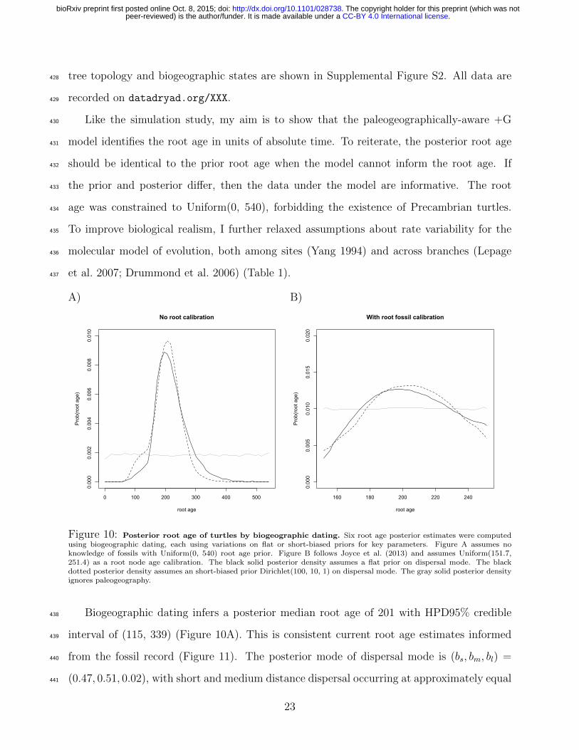
Like the simulation study, my aim is to show that the paleogeographically-aware +G430

model identifies the root age in units of absolute time. To reiterate, the posterior root age431

should be identical to the prior root age when the model cannot inform the root age. If432

the prior and posterior differ, then the data under the model are informative. The root433

age was constrained to Uniform(0, 540), forbidding the existence of Precambrian turtles.434

To improve biological realism, I further relaxed assumptions about rate variability for the435

molecular model of evolution, both among sites (Yang 1994) and across branches (Lepage436

et al. 2007; Drummond et al. 2006) (Table 1).437

A) B)

0 100 200 300 400 500

0.000

0.002

0.004

0.006

0.008

0.010

No root calibration

root age

Pro

b(ro

ot a

ge)

160 180 200 220 240

0.000

0.005

0.010

0.015

0.020

With root fossil calibration

root age

Pro

b(ro

ot a

ge)

Figure 10: Posterior root age of turtles by biogeographic dating. Six root age posterior estimates were computedusing biogeographic dating, each using variations on flat or short-biased priors for key parameters. Figure A assumes noknowledge of fossils with Uniform(0, 540) root age prior. Figure B follows Joyce et al. (2013) and assumes Uniform(151.7,251.4) as a root node age calibration. The black solid posterior density assumes a flat prior on dispersal mode. The blackdotted posterior density assumes an short-biased prior Dirichlet(100, 10, 1) on dispersal mode. The gray solid posterior densityignores paleogeography.

Biogeographic dating infers a posterior median root age of 201 with HPD95% credible438

interval of (115, 339) (Figure 10A). This is consistent current root age estimates informed439

from the fossil record (Figure 11). The posterior mode of dispersal mode is (bs, bm, bl) =440

(0.47, 0.51, 0.02), with short and medium distance dispersal occurring at approximately equal441

23


datadryad.org/XXX

http://dx.doi.org/10.1101/028738


0

200

400

Uni

form

(0, 5

40), −G

Uni

form

(0, 5

40),

+G, f

lat

Uni

form

(0, 5

40),

+G, s

hort

Uni

form

(151

, 251

), −G

Uni

form

(151

, 251

), +G

, fla

t

Uni

form

(151

, 251

), +G

, sho

rt

Joyc

e 07

Ste

rli e

t al 1

3

Dan

ilov

& P

arha

m 0

8

(nt)

Hug

all e

t al 0

7

(*) W

arno

ck e

t al 1

5

Joyc

e et

al 1

3

(aa)

Hug

all e

t al 0

7

Alfa

ro e

t al 0

9

Dor

nbur

g et

al 1

1

Model or study

Roo

t age

est

imat

es

Figure 11: Root age comparison. Root age estimates are presented both for analysis conducted for this manuscriptand as reported in existing publications. Existing estimates are as reported in Sterli et al. (2013) and supplemented recentlyreported results. Points and whiskers correspond to the point estimates and estimate confidence, which varies across analyses.The six left estimates were computed using biogeographic dating, each using variations on flat or short-biased priors for keyparameters. Two of these analyses ignore paleogeography (–G) so the posterior root age is the uniform prior root age, whosemode (not shown) equals all values supported by the prior. Hugall et al. (2007) reports ages for analyses using amino acids (aa)and nucleotides (nt). Warnock et al. (2015) reports many estimates while exploring prior sensitivity, but only uniform priorresults are shown here.

rates and long distance dispersal being rare by comparison. Biogeographic events occurred at442

a ratio of about 6:1 when compared to molecular events (posterior means: µx = 1.9E−3, µz =443

1.1E−2). The posterior mode tree height measured in expected number of dispersal events444

is 2.3 with HPD95% (1.5, 3.0), i.e. as a treewide average, the current location of each taxon445

is the result of about two dispersal events.446

The flat prior distribution for competing dispersal modes is Dirichlet(1, 1, 1) and does not447

capture the intuition that short distance dispersal should be far more common than long dis-448

tance dispersal. I encoded this intuition in the dispersal mode prior, setting the distribution449

24


http://dx.doi.org/10.1101/028738


to Dirichlet(100, 10, 1), which induces expected proportion of 100:10:1 short:medium:long450

dispersal events. After re-analyzing the data with the short-biased dispersal prior, the poste-451

rior median and HPD95% credible interval were estimated to be, respectively, 204 (96, 290)452

(Figure 10A).453

Biogeographic dating is compatible with fossil dating methods, so I repeated the analysis454

for both flat and informative prior dispersal modes while substituting the Uniform(0, 540)455

prior on root age calibration for Uniform(151.7, 251.4) (Joyce et al. 2013). When taking456

biogeography into account, the model more strongly disfavors post-Pangaean origins for the457

clade than when biogeography is ignored, but the effect is mild. Posterior distributions of458

root age was relatively insensitive to the flat and short-biased dispersal mode priors, with459

posterior medians and credible intervals of 203 (161, 250) and 208 (159, 250), respectively.460

A) B)

Prob(area)

Mod

el o

r dat

a

Unif(151, 251), +G, shortUnif(151, 251), +G, flat Unif(151, 251), −G

Unif(0, 540), +G, shortUnif(0, 540), +G, flat Unif(0, 540), −G

Tip state frequencies

S. A

mer

ica

(N)

S. A

mer

ica

(E)

S. A

mer

ica

(S)

N. A

mer

ica

(NW

)N

. Am

eric

a (S

E)

N. A

mer

ica

(NE

)N

. Am

eric

a (S

W)

Greenland

Europe

Asi

a (C

)A

sia

(E)

Asi

a (S

E)

Asi

a (N

E)

Afri

ca (W

)A

frica

(S)

Afri

ca (E

)A

frica

(N)

Aus

tralia

(N)

Aus

tralia

(S)

India

Madagascar

Ant

arct

ica

(W)

Ant

arct

ica

(E)

Mal

aysi

an A

rch.

New

Zea

land

0.0

0.2

0.4

0.6

0.8

1.0

Prob(area)

Pro

b(ro

ot a

ge)

020406080100120140160180200220240260280300320340360380400420440460480500520

S. A

mer

ica

(N)

S. A

mer

ica

(E)

S. A

mer

ica

(S)

N. A

mer

ica

(NW

)N

. Am

eric

a (S

E)

N. A

mer

ica

(NE

)N

. Am

eric

a (S

W)

Greenland

Europe

Asi

a (C

)A

sia

(E)

Asi

a (S

E)

Asi

a (N

E)

Afri

ca (W

)A

frica

(S)

Afri

ca (E

)A

frica

(N)

Aus

tralia

(N)

Aus

tralia

(S)

India

Madagascar

Ant

arct

ica

(W)

Ant

arct

ica

(E)

Mal

aysi

an A

rch.

New

Zea

land

0.00

0.02

0.04

0.06

0.08

0.10

0.12

0.14

0.16

Figure 12: Root state estimates. A) Posterior probabilities of root state are given for the six empirical analyses. B)Joint-marginal posterior probabilities of root age and root state are given for the empirical analysis without a root calibrationand with a flat dispersal mode prior. Root ages are binned into intervals of width 20.

All posterior root state estimates favored South America (N) for the paleogeographically-461

informed analyses (Figure 12A). Although this is in accord with the root node calibration462

adopted from Joyce et al. (2013)—Caribemys oxfordiensis, sampled from Cuba, and the463

oldest accepted crown group testudine—the fossil is described as a marine turtle, so the464

accordance may simply be coincidence. In contrast, the paleogeographically-naive models465

25


http://dx.doi.org/10.1101/028738


support Southeast Asian origin of Testudines, where, incidentally, Southeast Asia is the most466

frequently inhabited area among the 185 testudines. For the analysis with a flat dispersal467

mode prior and no root age calibration, all root states with high posterior probability appear468

to concur on the posterior root age density (Figure 12B), i.e. regardless of conditioning on469

South America (N), North America (SE), or North America (SW) as a root state, the470

posterior root age density is roughly equal.471

4 Discussion472

The major obstacle preventing the probabilistic union of paleogeographical knowledge,473

biogeographic inference, and divergence time estimation has been methodological, which I474

have attempted to redress in this manuscript. The intuition justifying prior-based fossil cali-475

brations (Parham et al. 2011), i.e. that fossil occurrences should somehow inform divergence476

times, has recently been formalized into several models (Pyron 2011; Ronquist et al. 2012;477

Heath et al. 2014). Here I present an analogous treatment for prior-based biogeographic478

calibrations, i.e. that biogeographic patterns of modern species echo time-calibrated paleo-479

biogeographic events, by describing how epoch models (Ree et al. 2005; Ree and Smith 2008;480

Bielejec et al. 2014) are informative of absolute divergence times. Briefly, I accomplished481

this using a simple time-heterogeneous dispersal process (Sanmartın et al. 2008), where482

dispersal rates are piecewise-constant, and determined by a graph-based paleogeographical483

model (Section 2.4). The paleogeographical model itself was constructed by translating var-484

ious published paleogeographical reconstructions (Figure 5) into a time-calibrated vector of485

dispersal graphs.486

Through simulation, I showed biogeographic dating identifies tree height from the rates487

of molecular and biogeographic character change. This simulation framework could easily be488

extended to investigate for what phylogenetic, paleogeographic, and biogeographic conditions489

one is able to reliably extract information for the root age. For example, a clade with taxa490

invariant for some biogeographic state would contain little to no information about root age,491

26


http://dx.doi.org/10.1101/028738


provided the area has always existed and had a constant number of dispersal edges over492

time. At the other extreme, a clade with a very high dispersal rate or with a proclivity493

towards long distance dispersal might provide little due to signal saturation (Figure 6C).494

The breadth of applicability of biogeographic dating will depend critically on such factors,495

but because we do not expect to see closely related species uniformly distributed about Earth496

nor in complete sympatry, that breadth may not be so narrow, especially in comparison to497

the fossil record.498

The majority of groups have poor fossil records, and biogeographic dating provides a499

second hope for dating divergence times. Since biogeographic dating does not rely on any500

fossilization process or data directly, it is readily compatible with existing fossil-based dating501

methods (Figure 10B). When fossils with geographical information are available, researchers502

have shown fossil taxa improve biogeographical analyses (Moore et al. 2008; Wood et al.503

2012). In principle, the biogeographic process should guide placement of fossils on the504

phylogeny, and the age of the fossils should improve the certainty in estimates of ances-505

tral biogeographic states (Slater et al. 2012), on which biogeographic dating relies. Joint506

inference of divergence times, biogeography, and fossilization stands to resolve recent paleo-507

biogeographic conundrums that may arise when considering inferences separately (Beaulieu508

et al. 2013; Wilf and Escapa 2014).509

Because time calibration through biogeographic inferences comes primarily from the pa-510

leogeographical record, not the fossil record, divergence times may be estimated from exclu-511

sively extant taxa under certain biogeographical and phylogenetic conditions. When fossils512

are available, however, biogeographic dating is compatible with other fossil-based dating513

methods (e.g. node calibrations, fossil tip dating, fossilized birth-death). As a proof of con-514

cept, I assumed a flat root age calibration prior for the origin time of turtles: the posterior515

root age was also flat when paleogeography was ignored, but Pangaean times of origin were516

strongly preferred when dispersal rates conditioned on paleogeography (Figure 10). Under517

the uninformative prior distributions on root age, biogeographic dating estimated turtles518

originated between the Mississipian (339 Ma) and Early Cretaceous (115 Ma) periods, with519

27


http://dx.doi.org/10.1101/028738


a median age of 201 Ma. Under an ignorance prior where short, medium, and long dis-520

tance dispersal events have equal prior rates, short and medium distance dispersal modes521

are strongly favored over long distance dispersal. Posterior estimates changed little by in-522

forming the prior to strongly prefer short distance dispersal. Both with and without root523

age calibrations, and with flat and biased dispersal mode priors, biogeographic dating placed524

the posterior mode origin time of turtles at approximately 210–200 Ma, which is consistent525

with fossil-based estimates (Figure 11).526

Model inadequacies and future extensions527

The simulated and empirical studies demonstrate biogeographic dating improves diver-528

gence time estimates, with and without fossil calibrations, but many shortcomings in the529

model remain to be addressed. When any model is misspecified, inference is expected to pro-530

duce uncertain, or worse, spurious results (Lemmon and Moriarty 2004), and biogeographic531

models are not exempted. I discuss some of the most apparent model misspecifications below.532

Anagenetic range evolution models that properly allow species inhabit multiple areas533

should improve the informativeness of biogeographic data. Imagine taxa T1 and T2 inhabit534

areas ABCDE and FGHIJ , respectively. Under the simple model assumed in this paper,535

the tip states are ambiguous with respect to their ranges, and for each ambiguous state only536

a single dispersal event is needed to reconcile their ranges. Under a pure anagenetic range537

evolution model (Ree et al. 2005), at least five dispersal events are needed for reconciliation.538

Additionally, some extant taxon ranges may span ancient barriers, such as a terrestrial539

species spanning both north and south of the Isthmus of Panama. This situation almost540

certainly requires a dispersal event to have occurred after the isthmus was formed when541

multiple-area ranges are used. For single-area species ranges coded as ambiguous states,542

the model is incapable of evaluating the likelihood that the species is found in both areas543

simultaneously, so additional information about the effects of the paleogeographical event544

on divergence times is potentially lost.545

Any model where the diversification process and paleogeographical states (and events)546

28


http://dx.doi.org/10.1101/028738


are correlated will obviously improve divergence time estimates so long as that relationship547

is biogeographically realistic. Although the repertoire of cladogenetic models is expanding548

in terms of types of transition events, they do not yet account for geographical features,549

such as continental adjacency or geographical distance. Incorporating paleogeographical550

structure into cladogenetic models of geographically-isolated speciation, such as vicariance551

(Ronquist 1997), allopatric speciation (Ree et al. 2005; Goldberg et al. 2011), and jump552

dispersal (Matzke 2014), is crucial not only to generate information for biogeographic dating553

analyses, but also to improve the accuracy of ancestral range estimates. Ultimately, cladoge-554

netic events are state-dependent speciation events, so the desired process would model range555

evolution jointly with the birth-death process (Maddison et al. 2007; Goldberg et al. 2011),556

but inference under these models for large state spaces is currently infeasible. Regardless,557

any cladogenetic range-division event requires a widespread range, which in turn implies it558

was preceeded by dispersal (range expansion) events. Thus, if we accept that paleogeogra-559

phy constrains the dispersal process, even a simple dispersal-only model will extract dating560

information when describing a far more complex evolutionary process.561

That said, the simple paleogeographical model described herein (Section 2.4) has many562

shortcomings itself. It is only designed for terrestrial species originating in the last 540563

Ma. Rates of dispersal between areas are classified into short, medium, and long distances,564

but with subjective criteria. The number of epochs and areas was limited by my ability to565

comb the literature for well-supported paleogeological events, while constrained by compu-566

tational considerations. The timing of events was assumed to be known perfectly, despite567

the literature reporting ranges of estimates. Certainly factors such as global temperature,568

precipitation, ecoregion type, etc. affect dispersal rates between areas, but were ignored. All569

of these factors can and should be handled more rigorously in future studies by modeling570

these uncertainties as part of a joint Bayesian analysis (Hohna et al. 2014).571

Despite these flaws, defining the paleogeographical model serves as an excercise to identify572

what features allow a biogeographic process to inform speciation times. Dispersal barriers are573

clearly clade-dependent, e.g. benthic marine species dispersal would be poorly modeled by574

29


http://dx.doi.org/10.1101/028738


the terrestrial graph. Since dispersal routes for the terrestrial graph might serve as dispersal575

barriers for a marine graph, there is potential for learning about mutually exclusive dispersal576

corridor use in a multi-clade analysis (Sanmartın et al. 2008). Classifying dispersal edges577

into dispersal mode classes may be made rigorous using clustering algorithms informed by578

paleogeographical features, or even abandoned in favor of modeling rates directly as functions579

of paleogeographical features like distance. Identifying significant areas and epochs remains580

challenging, where presumably more areas and epochs are better to approximate continu-581

ous space and time, but this is not without computational challenges (Ree and Sanmartın582

2009; Webb and Ree 2012; Landis et al. 2013). Rather than fixing epoch event times to583

point estimates, one might assign empirical prior distributions based on collected estimates.584

Ideally, paleogeographical event times and features would be estimated jointly with phyloge-585

netic evidence, which would require interfacing phylogenetic inference with paleogeographical586

inference. This would be a profitable, but substantial, interdisciplinary undertaking.587

Conclusion588

Historical biogeography is undergoing a probabilistic renaissance, owing to the abundance589

of georeferenced biodiversity data now hosted online and the explosion of newly published590

biogeographic models and methods (Ree et al. 2005; Ree and Smith 2008; Sanmartın et al.591

2008; Lemmon and Lemmon 2008; Lemey et al. 2010; Goldberg et al. 2011; Webb and592

Ree 2012; Landis et al. 2013; Matzke 2014; Tagliacollo et al. 2015). Making use of these593

advances, I have shown how patterns latent in biogeographic characters, when viewed with594

a paleogeographic perspective, provide information about the geological timing of speciation595

events. The method conditions directly on biogeographic observations to induce dated node596

age distributions, rather than imposing (potentially incorrect) beliefs about speciation times597

using node calibration densities, which are data-independent prior densities. Biogeographic598

dating may present new opportunities for dating phylogenies for fossil-poor clades since599

the technique requires no fossils. This establishes that historical biogeography has untapped600

practical use for statistical phylogenetic inference, and should not be considered of secondary601

30


http://dx.doi.org/10.1101/028738


interest, only to be analysed after the species tree is estimated.602

Acknowledgements603

I thank Tracy Heath, Sebastian Hohna, Josh Schraiber, Lucy Chang, Pat Holroyd, Nick604

Matzke, Michael Donoghue, and John Huelsenbeck for valuable feedback, support, and en-605

couragement regarding this work. I also thank James Albert, Alexandre Antonelli, and the606

Society of Systematic Biologists for inviting me to present this research at Evolution 2015607

in Guaruja, Brazil. Simulation analyses were computed using XSEDE, which is supported608

by National Science Foundation grant number ACI-1053575.609

Funding610

MJL was supported by a National Evolutionary Synthesis Center Graduate Fellowship611

and a National Institutes of Health grant (R01-GM069801) awarded to John P. Huelsenbeck.612

31


http://dx.doi.org/10.1101/028738


613

References614

Alfaro, M. E., F. Santini, C. Brock, H. Alamillo, A. Dornburg, D. L. Rabosky, G. Carnevale,615

and L. J. Harmon. 2009. Nine exceptional radiations plus high turnover explain species616

diversity in jawed vertebrates. Proceedings of the National Academy of Sciences 106:13410–617

13414.618

Beaulieu, J. M., D. C. Tank, and M. J. Donoghue. 2013. A southern hemisphere origin for619

campanulid angiosperms, with traces of the break-up of gondwana. BMC Evolutionary620

Biology 13:80.621

Behrensmeyer, A. K., S. M. Kidwell, and R. A. Gastaldo. 2000. Taphonomy and paleobiology.622

Paleobiology 26:103–147.623

Bielejec, F., P. Lemey, G. Baele, A. Rambaut, and M. A. Suchard. 2014. Inferring heteroge-624

neous evolutionary processes through time: from sequence substitution to phylogeography.625

Systematic Biology 63:493–504.626

Blakey, R. 2006. Global paleogeographic views of earth history: Late Precambrian to Recent.627

R. Blakey.628

Boyden, J. A., R. D. Muller, M. Gurnis, T. H. Torsvik, J. A. Clark, M. Turner, H. Ivey-Law,629

R. J. Watson, and J. S. Cannon. 2011. Next-generation plate-tectonic reconstructions using630

gplates. Geoinformatics: cyberinfrastructure for the solid earth sciences Pages 95–114.631

Buerki, S., F. Forest, N. Alvarez, J. A. A. Nylander, N. Arrigo, and I. Sanmartın. 2011.632

An evaluation of new parsimony-based versus parametric inference methods in biogeog-633

raphy: a case study using the globally distributed plant family Sapindaceae. Journal of634

Biogeography 38:531–550.635

Carlquist, S. 1966. The biota of long-distance dispersal. i. principles of dispersal and evolu-636

tion. Quarterly Review of Biology Pages 247–270.637

32


http://dx.doi.org/10.1101/028738


Crawford, N. G., J. F. Parham, A. B. Sellas, B. C. Faircloth, T. C. Glenn, T. J. Papenfuss,638

J. B. Henderson, M. H. Hansen, and B. W. Simison. 2015. A phylogenomic analysis of639

turtles. Molecular Phylogenetics and Evolution 83:250–257.640

Danilov, I. G. and J. F. Parham. 2008. A reassessment of some poorly known turtles from641

the middle jurassic of china, with comments on the antiquity of extant turtles. Journal of642

Vertebrate Paleontology 28:306–318.643

Dornburg, A., J. M. Beaulieu, J. C. Oliver, and T. J. Near. 2011. Integrating fossil preser-644

vation biases in the selection of calibrations for molecular divergence time estimation.645

Systematic Biology 60:519–527.646

Drummond, A. J., S. Y. Ho, M. J. Phillips, and A. Rambaut. 2006. Relaxed phylogenetics647

and dating with confidence. PLoS Biology 4:e88.648

Edgar, R. C. 2004. MUSCLE: Multiple sequence alignment with high accuracy and high649

throughput. Nucleic Acids Research 32:1792–1797.650

Felsenstein, J. 1981. Evolutionary trees from DNA sequences: A maximum likelihood ap-651

proach. Journal of Molecular Evolution 17:368–376.652

Gavryushkina, A., T. A. Heath, D. T. Ksepka, T. Stadler, D. Welch, and A. J. Drummond.653

2015. Bayesian total evidence dating reveals the recent crown radiation of penguins. arXiv654

preprint arXiv:1506.04797 .655

Gelman, A. and D. B. Rubin. 1992. Inferences from iterative simulation using multiple656

sequences. Statistical Science 7:457–511.657

Goldberg, E. E., L. T. Lancaster, and R. H. Ree. 2011. Phylogenetic inference of reciprocal658

effects between geographic range evolution and diversification. Systematic Biology 60:451–659

465.660

Guillon, J.-M., L. Guery, V. Hulin, and M. Girondot. 2012. A large phylogeny of turtles661

(testudines) using molecular data. Contributions to Zoology 81:147–158.662

33


http://dx.doi.org/10.1101/028738


Gurnis, M., M. Turner, S. Zahirovic, L. DiCaprio, S. Spasojevic, R. D. Muller, J. Boy-663

den, M. Seton, V. C. Manea, and D. J. Bower. 2012. Plate tectonic reconstructions with664

continuously closing plates. Computers & Geosciences 38:35–42.665

Heads, M. 2005. Dating nodes on molecular phylogenies: a critique of molecular biogeogra-666

phy. Cladistics 21:62–78.667

Heads, M. 2011. Old taxa on young islands: a critique of the use of island age to date668

island-endemic clades and calibrate phylogenies. Systematic Biology 60:204–218.669

Heath, T. A., J. P. Huelsenbeck, and T. Stadler. 2014. The fossilized birth–death process for670

coherent calibration of divergence-time estimates. Proceedings of the National Academy671

of Sciences 111:E2957–E2966.672

Heled, J. and A. J. Drummond. 2012. Calibrated tree priors for relaxed phylogenetics and673

divergence time estimation. Systematic Biology 61:138–149.674

Ho, S. Y., K. J. Tong, C. S. Foster, A. M. Ritchie, N. Lo, and M. D. Crisp. 2015. Biogeo-675

graphic calibrations for the molecular clock. Biology letters 11:20150194.676

Ho, S. Y. W. and M. J. Phillips. 2009. Accounting for calibration uncertainty in phylogenetic677

estimation of evolutionary divergence times. Systematic Biology 58:367–380.678

Hohna, S., T. A. Heath, B. Boussau, M. J. Landis, F. Ronquist, and J. P. Huelsenbeck.679

2014. Probabilistic graphical model representation in phylogenetics. Systematic Biology680

63:753–771.681

Hugall, A. F., R. Foster, and M. S. Y. Lee. 2007. Calibration choice, rate smoothing, and the682

pattern of tetrapod diversification according to the long nuclear gene rag-1. Systematic683

Biology 56:543–563.684

Joyce, W. G. 2007. Phylogenetic relationships of mesozoic turtles. Bulletin of the Peabody685

Museum of Natural History 48:3–102.686

34


http://dx.doi.org/10.1101/028738


Joyce, W. G., J. F. Parham, T. R. Lyson, R. C. M. Warnock, and P. C. J. Donoghue. 2013. A687

divergence dating analysis of turtles using fossil calibrations: an example of best practices.688

Journal of Paleontology 87:612–634.689

Kidwell, S. M. and S. M. Holland. 2002. The quality of the fossil record: implications for690

evolutionary analyses. Annual Review of Ecology and Systematics Pages 561–588.691

Kodandaramaiah, U. 2011. Tectonic calibrations in molecular dating. Current Zoology692

57:116–124.693

Landis, M. J., N. J. Matzke, B. R. Moore, and J. P. Huelsenbeck. 2013. Bayesian analysis of694

biogeography when the number of areas is large. Systematic Biology 62:789–804.695

Lemey, P., A. Rambaut, A. J. Drummond, and M. A. Suchard. 2009. Bayesian phylogeogra-696

phy finds its roots. PLoS Computational Biology 5:e1000520.697

Lemey, P., A. Rambaut, J. J. Welch, and M. A. Suchard. 2010. Phylogeography takes a698

relaxed random walk in continuous space and time. Moleculate Biology and Evolution699

27:1877–1885.700

Lemmon, A. A. and E. M. Lemmon. 2008. A likelihood framework for estimating phylogeo-701

graphic history on a continuous landscape. Systematic Biology 57:544–561.702

Lemmon, A. R. and E. C. Moriarty. 2004. The importance of proper model assumption in703

bayesian phylogenetics. Systematic Biology 53:265–277.704

Lepage, T., D. Bryant, H. Philippe, and N. Lartillot. 2007. A general comparison of relaxed705

molecular clock models. Molecular Biology and Evolution 24:2669–2680.706

Maddison, W. P., P. E. Midford, and S. P. Otto. 2007. Estimating a binary character’s effect707

on speciation and extinction. Systematic Biology 56:701–710.708

Martin, A. P. and S. R. Palumbi. 1993. Body size, metabolic rate, generation time, and the709

molecular clock. Proceedings of the National Academy of Sciences 90:4087–4091.710

35


http://dx.doi.org/10.1101/028738


Matzke, N. J. 2014. Model selection in historical biogeography reveals that founder-event711

speciation is a crucial process in island clades. Systematic Biology Page syu056.712

Moore, B. R., S. A. Smith, R. H. Ree, and M. J. Donoghue. 2008. Incorporating fossil data713

in biogeographic inference: A likelihood approach. Evolution .714

Nylander, J. A., U. Olsson, P. Alstrom, and I. Sanmartın. 2008. Accounting for phylogenetic715

uncertainty in biogeography: a bayesian approach to dispersal-vicariance analysis of the716

thrushes (aves: Turdus). Systematic Biology 57:257–268.717

Parham, J. F., P. C. J. Donoghue, C. J. Bell, T. D. Calway, J. J. Head, P. A. Holroyd, J. G.718

Inoue, R. B. Irmis, W. G. Joyce, D. T. Ksepka, J. S. L. Patane, N. D. Smith, J. E. Tarver,719

M. van Tuinen, Z. Yang, K. D. Angielczyk, J. M. Greenwood, C. A. Hipsley, L. Jacobs,720

P. J. Makovicky, J. Muller, K. T. Smith, J. M. Theodor, and R. C. M. Warnock. 2011.721

Best practices for justifying fossil calibrations. Systematic Biology Page syr107.722

Passalacqua, N. G. 2015. On the definition of element, chorotype and component in biogeog-723

raphy. Journal of Biogeography 42:611–618.724

Plummer, M., N. Best, K. Cowles, and K. Vines. 2006. CODA: Convergence diagnosis and725

output analysis for MCMC. R News Pages 7–11.726

Pyron, R. A. 2011. Divergence time estimation using fossils as terminal taxa and the origins727

of lissamphibia. Systematic Biology 60:466–481.728

Ree, R. H., B. R. Moore, C. O. Webb, and M. J. Donoghue. 2005. A likelihood framework for729

inferring the evolution of geographic range on phylogenetic trees. Evolution 59:2299–2311.730

Ree, R. H. and I. Sanmartın. 2009. Prospects and challenges for parametric models in his-731

torical biogeographical inference. Journal of Biogeography 36:1211–1220.732

Ree, R. H. and S. A. Smith. 2008. Maximum likelihood inference of geographic range evolu-733

tion by dispersal, local extinction, and cladogenesis. Systematic Biology 57:4–14.734

36


http://dx.doi.org/10.1101/028738


Renner, S. S. 2005. Relaxed molecular clocks for dating historical plant dispersal events.735

Trends in Plant Science 10:550–558.736

Rodrigue, N. and H. Philippe. 2010. Mechanistic revisions of phenomenological modeling737

strategies in molecular evolution. Trends in Genetics 26:248–252.738

Ronquist, F. 1997. Dispersal-vicariance analysis: a new approach to the quantification of739

historical biogeography. Systematic Biology 46:195–203.740

Ronquist, F., S. Klopfstein, L. Vilhelmsen, S. Schulmeister, D. L. Murray, and A. P. Rasnit-741

syn. 2012. A total-evidence approach to dating with fossils, applied to the early radiation742

of the hymenoptera. Systematic Biology 61:973–999.743

Sanmartın, I., P. V. D. Mark, and F. Ronquist. 2008. Inferring dispersal: a bayesian approach744

to phylogeny-based island biogeography, with special reference to the canary islands. Jour-745

nal of Biogeography 35:428–449.746

Slater, G. J., L. J. Harmon, and M. E. Alfaro. 2012. Integrating fossils with molecular747

phylogenies improves inference of trait evolution. Evolution 66:3931–3944.748

Sterli, J., D. Pol, and M. Laurin. 2013. Incorporating phylogenetic uncertainty on phylogeny-749

based palaeontological dating and the timing of turtle diversification. Cladistics 29:233–750

246.751

Tagliacollo, V. A., S. M. Duke-Sylvester, W. A. Matamoros, P. Chakrabarty, and J. S.752

Albert. 2015. Coordinated dispersal and pre-isthmian assembly of the central american753

ichthyofauna. Systematic Biology Page syv064.754

Thorne, J., H. Kishino, and I. S. Painter. 1998. Estimating the rate of evolution of the rate755

of molecular evolution. Molecular Biology and Evolution 15:1647–1657.756

Towns, J., T. Cockerill, M. Dahan, I. Foster, K. Gaither, A. Grimshaw, V. Hazlewood,757

S. Lathrop, D. Lifka, G. D. Peterson, et al. 2014. Xsede: Accelerating scientific discovery.758

Computing in Science & Engineering 16:62–74.759

37


http://dx.doi.org/10.1101/028738


Warnock, R. C., J. F. Parham, W. G. Joyce, T. R. Lyson, and P. C. J. Donoghue. 2015.760

Calibration uncertainty in molecular dating analyses: there is no substitute for the prior761

evaluation of time priors. Proceedings of the Royal Society of London B: Biological Sciences762

282:20141013.763

Webb, C. O. and R. H. Ree. 2012. Historical biogeography inference in Malesia. Pages 191–764

215 in Biotic evolution and environmental change in Southeast Asia (D. Gower, K. John-765

son, J. Richardson, B. Rosen, L. Ruber, and S. Williams, eds.) Cambridge University766

Press.767

Wilf, P. and I. H. Escapa. 2014. Green web or megabiased clock? plant fossils from gond-768

wanan patagonia speak on evolutionary radiations. New Phytologist 207:283–290.769

Wolfe, K. H., W.-H. Li, and P. M. Sharp. 1987. Rates of nucleotide substitution vary greatly770

among plant mitochondrial, chloroplast, and nuclear dnas. Proceedings of the National771

Academy of Sciences 84:9054–9058.772

Wood, H. M., N. J. Matzke, R. G. Gillespie, and C. E. Griswold. 2012. Treating fossils773

as terminal taxa in divergence time estimation reveals ancient vicariance patterns in the774

palpimanoid spiders. Systematic Biology 62:264–284.775

Yang, Z. 1994. Maximum likelihood phylogenetic estimation from DNA sequences with vari-776

able rates over sites: Approximate methods. Journal of Molecular Evolution 39:306–314.777

Zuckerkandl, E. and L. Pauling. 1962. Molecular disease, evolution, and genetic heterogene-778

ity. Pages 189–225 in Horizons in Biochemistry (M. Kasha and B. Pullman, eds.) Academic779

Press, New York.780

38


http://dx.doi.org/10.1101/028738


Documents

Biogeographic dating of speciation times using ... · 22 stochastic process may be used to estimate absolute ... I analyze the well-studied turtle ... 92 nario as a calibration point