Embed Size (px)
Citation preview

Syst. Biol. 66(2):128–144, 2017© The Author(s) 2016. Published by Oxford University Press, on behalf of the Society of Systematic Biologists. All rights reserved.For Permissions, please email: [email protected]:10.1093/sysbio/syw040Advance Access publication May 6, 2016
Biogeographic Dating of Speciation Times Using Paleogeographically Informed Processes
MICHAEL J. LANDIS1,2,∗1Department of Integrative Biology, University of California, Berkeley, CA 94720, USA; 2Department of Ecology and Evolutionary Biology,
Yale University, New Haven, CT 06520, USA;∗Correspondence to be sent to: Department of Ecology and Evolutionary Biology, Yale University, New Haven, CT 06520, USA;
E-mail: [email protected]
Received 8 October 2015; reviews returned 26 April 2016; accepted 28 April 2016Associate Editor: Emma Goldberg
Abstract.—Standard models of molecular evolution cannot estimate absolute speciation times alone, and require externalcalibrations to do so, such as fossils. Because fossil calibration methods rely on the incomplete fossil record, a great numberof nodes in the tree of life cannot be dated precisely. However, many major paleogeographical events are dated, and sincebiogeographic processes depend on paleogeographical conditions, biogeographic dating may be used as an alternativeor complementary method to fossil dating. I demonstrate how a time-stratified biogeographic stochastic process may beused to estimate absolute divergence times by conditioning on dated paleogeographical events. Informed by the currentpaleogeographical literature, I construct an empirical dispersal graph using 25 areas and 26 epochs for the past 540 Ma ofEarth’s history. Simulations indicate biogeographic dating performs well so long as paleogeography imposes constraint onbiogeographic character evolution. To gauge whether biogeographic dating may be of practical use, I analyzed the well-studied turtle clade (Testudines) to assess how well biogeographic dating fares when compared to fossil-calibrated datingestimates reported in the literature. Fossil-free biogeographic dating estimated the age of the most recent common ancestor ofextant turtles to be from the Late Triassic, which is consistent with fossil-based estimates. Dating precision improves furtherwhen including a root node fossil calibration. The described model, paleogeographical dispersal graph, and analysis scriptsare available for use with RevBayes. [biogeography, phylogenetics, paleogeography, tree-dating, Testudines, Bayesian.]
Time is a simple and fundamental axis of evolution.Knowing the order and timing of evolutionary eventsgrants us insight into how vying evolutionary processesinteract. With a perfectly accurate catalog of geologicallydated speciation times, many macroevolutionaryquestions would yield to simple interrogation, suchas whether one clade exploded with diversity beforeor after a niche-analogous clade went extinct, orwhether some number of contemporaneous biota wereeradicated simultaneously by the same mass extinctionevent. Only rarely does the fossil record give audience tothe exact history of evolutionary events: it is infamouslyirregular across time, space, and species, so biologistsgenerally resort to inference to estimate when, where,and what happened to fill those gaps. That said, we havenot yet found a perfect character or model to infer datesfor divergence times, so advances in dating strategiesare urgently needed. A brief survey of the field revealswhy.
The molecular clock hypothesis of Zuckerkandl andPauling (1962) states that if substitutions arise (i.e.,alleles fix) at a constant rate, the expected number ofsubstitutions is the product of the substitution rate andthe time the substitution process has been operating.With data from extant taxa, we only observe the outcomeof the evolutionary process for an unknown rate and anunknown amount of time. In this case, rate and timeare not separately identifiable, so they are estimated astheir product, a compound parameter called length. Ifall species evolved under a single rate (a strict clock),a phylogeny with branches measured in lengths wouldgive relative divergence times, that is, proportionalto absolute divergence times. The same is true whensubstitution rates vary across lineages (Wolfe et al. 1987;Martin and Palumbi 1993) and relaxed clock models are
applied (Thorne et al. 1998; Drummond et al. 2006): onlyrelative times may be estimated. Extrinsic information,for example, a dated calibration density, is needed toestablish an absolute timescale, and typically takes formas a fossil occurrence or paleogeographical event.
Fossils may be used in several ways to calibratedivergence times. The simplest method is the fossil nodecalibration, whereby the fossil is associated with a cladeto constrain its time of origin (Ho and Phillips 2009;Parham et al. 2012). Node calibrations are empiricalpriors, not data-dependent stochastic processes, so theydepend on experts’ abilities to quantify the distributionof plausible ages for the given node. That is, nodecalibrations do not arise from a generative evolutionaryprocess, so the posterior timescale is entirely determinedby how the prior is specified. Rather than usingprior node calibrations, fossil tip-dating (Pyron 2011;Ronquist et al. 2012) treats fossil occurrences as terminaltaxa with morphological characters as part of anystandard phylogenetic analysis. The tree prior andmodel of morphological evolution are jointly appliedto date speciation times from the fossils’ ages andmorphological data. Introducing a generative process offossilization, Heath et al. (2014) developed the fossilizedbirth–death process, by which lineages speciate, goextinct, or produce fossil observations. Using fossil tip-dating with the fossilized birth–death process, Zhanget al. (2015) and Gavryushkina et al. (2015) demonstratedmultiple calibration techniques may be used in tandemin a theoretically consistent framework (i.e. withoutintroducing model violation).
Of course, fossil calibrations require fossils, but manyclades leave few to no known fossils due to taphonomicprocesses, which filter out species with soft or fragiletissues, or with tissues that were buried in substrates
128

2017 LANDIS—BIOGEOGRAPHIC DATING OF SPECIATION TIMES 129
that were too humid, too arid, or too rocky; or due tosampling biases, such as geographical or political biasesimbalancing collection efforts (Behrensmeyer et al. 2000;Kidwell and Holland 2002). Although these biases do notprohibitively obscure the record for widespread specieswith robust mineralized skeletons—as is the case formany marine invertebrate and large vertebrate groups—fossil-free calibration methods are desperately needed todate the remaining majority of nodes in the tree of life.
In this direction, analogous to fossil node-dating,node dates may be calibrated using paleobiogeographicscenarios (Heads 2005; Renner 2005). An ornithologist,for example, might reasonably argue that a bird knownas endemic to a young island may have speciatedonly after the island was created, thus providing amaximum age of origin. However, using this scenarioas a calibration excludes the possibility of alternativehistorical biogeographic explanations, for example, thebird might have speciated off-island before the islandsurfaced and migrated there afterward; see Heads (2005,2011), Kodandaramaiah (2011), and Ho et al. (2015) fordiscussion on the uses and pitfalls of biogeographicnode calibrations. Biogeographic node calibrations, likefossil node calibrations, fundamentally rely on someprior distribution of divergence times. This complicatesmodel comparison since prior-encoded beliefs varyfrom expert to expert. Worsening matters, the timeand context of biogeographic events are never directlyobserved, so asserting that a particular dispersal eventinto an island system resulted in a speciation eventto calibrate a node fails to account for the uncertaintythat the assumed evolutionary scenario took placeat all. When estimating ancestral states, phylogeniesdated by biogeographic node calibrations should beavoided, for fear of producing falsely confident resultsby “double counting” the data: once when justifyingthe node calibrations and again when performingthe biogeographic inference. Ideally, to avoid theseproblems, all possible biogeographic and diversificationscenarios would be considered jointly, with eachscenario given credence in proportion to its probability.
Inspired by advents in fossil dating models (Pyron2011; Ronquist et al. 2012; Heath et al. 2014),which have matured from phenomenological towardmechanistic approaches (Rodrigue and Philippe 2010), Ipresent an explicitly data-dependent and process-basedbiogeographic method for divergence time dating toformalize the intuition underlying biogeographic nodecalibrations. Analogous to fossil tip-dating, the goal isto allow the observed biogeographic states at the “tips”of the tree to induce a posterior distribution of datedspeciation times by way of an evolutionary process.By modeling dispersal rates between areas as subjectto time-calibrated paleogeographical information, suchas the merging and splitting of continental adjacenciesdue to tectonic drift, particular dispersal events betweenarea-pairs are expected to occur with higher probabilityduring certain geological time intervals than duringothers. For example, the dispersal rate between SouthAmerica and Africa was likely to be higher when they
were joined as West Gondwana (ca. 120 Ma) than whenseparated as they are today. If the absolute timing ofdispersal events on a phylogeny matters, then so mustthe absolute timing of divergence events. Unlike fossiltip-dating, biogeographic dating should, in principle, beable to date speciation times only using extant taxa.
To illustrate how this is possible, I construct atoy biogeographic example to demonstrate whenpaleogeography may date divergence times, thenfollow with a more formal description of the model.By performing joint inference with molecular andbiogeographic data, I demonstrate the effectivenessof biogeographic dating by applying it to simulatedand empirical scenarios, showing rate and time areidentifiable. While researchers have accounted forphylogenetic uncertainty in biogeographic analyses(Nylander et al. 2008; Lemey et al. 2009; Beaulieuet al. 2013), I am unaware of work demonstratinghow paleogeographic calibrations may be leveraged todate divergence times via a biogeographic process. Forthe empirical analysis, I date the divergence times forTestudines using biogeographic dating, first without anyfossils, then using a fossil root node calibration. Finally,I discuss the strengths and weaknesses of the method,and how it may be improved in future work.
MODEL
The Anatomy of Biogeographic DatingBriefly, I will introduce an example of how
time-calibrated paleogeographical events may impartinformation through a biogeographic process to datespeciation times, then later develop the detailsunderlying the strategy, which I refer to as biogeographicdating. Throughout the article, I assume a rootedphylogeny with known topology but with unknowndivergence times that I wish to estimate. Time ismeasured in geological units and as time until present,with t=0 being the present, t<0 being the past, andage being the negative amount of time until present.To keep the model of biogeographic evolution simple,the observed taxon occurrence matrix is assumed tobe generated by a discrete-valued dispersal processwhere each taxon is present in only a single area ata time (Sanmartín et al. 2008). For example, taxon T1might be coded to be found in area A or area B, butnot both simultaneously. Although basic, this model issufficient to make use of paleogeographical information,suggesting more realistic models will fare better.
Consider two areas, A and B, that drift into and out ofcontact over time. When in contact, dispersal is possible;when not, impossible. The dispersal rate between A andB equals one when the disperal route exists, and equalszero when it does not. When A and B have a dispersalrate of zero, because the two areas are not connectedby alternate dispersal routes, however circuitous, theprobability of transitioning from area A to area B equalszero no matter how much time elapses. Under thisconstruction, certain types of dispersal events are more

130 SYSTEMATIC BIOLOGY VOL. 66
c)a)
d)b)A T1
T2
T3
A
B
A T1
T2
T3
A
BA→B
A→B
A
A
s t
s t
τ
τ
P>0
P=0
A
T1
T2
T3A→B B
B
A
A
T1
T2
T3A→B B
B
A
T4
T4
A
A
s t
s t
τ
τ
P>0
P=0
FIGURE 1. Biogeographic dating toy example. Two paleogeographic scenarios are given: a split event (a and b) and a merge event (c and d).Scenarios assume only a single dispersal event occurs for a given branch (see text). a, b) T1 and T2 have state A and the transition A→B mostparsimoniously explains how T3 has state B. The transition probabilty for P=[P(s,t)]AB is nonzero before the paleogeographical split event attime �, and is zero afterward. Two possible divergence and dispersal times are given: a) T3 originates before the split when the transition A→Bhas nonzero probability. b) T3 originates after the split when the transition A→B has probability zero. c, d) T1 and T2 have the state A andthe transition A→B on the lineage leading to (T3,T4) most parsimoniously explains how T3 and T4 have state B. The transition probabilty forP=[P(s,t)]AB is zero before the paleogeographical merge event at time �, and only nonzero afterward. Two possible divergence and dispersaltimes are given: c) T3 and T4 originate after the merge when the transition A→B has nonzero probability. d) T3 and T4 originate before themerge when the transition A→B has probability zero.
likely to occur during certain absolute (not relative) timeintervals, which potentially influences probabilities ofdivergence times in absolute units.
In practice, biogeographic dating requires threesources of data: molecular data to accurately estimatethe relative branch lengths and (if desired) topologyof a rooted species tree, biogeographic data to informthe biogeographic process that in turn informs thebranch lengths in absolute time, and an empiricalpaleogeographic model that alters the rates ofbiogeographic change over time. As later described inthe “Analysis” section, these data are jointly analyzedin a Bayesian framework using RevBayes (Höhna et al.2014), but the general concept is not wed to a particularinference methodology.
Below, I give examples of when a key divergence eventis likely to precede a split event (Figs. 1a,b) or to followa merge event (Figs. 1c,d). To simplify matters withoutcompromising the general logic of the method, I assumeonly a single change occurs on a particular branchgiven the topology and tip states. In this sense, the toyexamples resemble parsimony reconstructions, exceptthey depend critically on branch length information.
In the first scenario (Figs. 1a,b), sister taxa T2 and T3are found in areas A and B, respectively. The divergence
time, s, is a random variable to be inferred. At time�, the dispersal route (A,B) is destroyed, inducing thetransition probability between areas A and B to equalzero between times � and 0. Since T2 and T3 are foundin different areas, at least one dispersal event musthave occurred during an interval of non-zero dispersalprobability. Then, the divergence event that gave rise toT2 and T3 must have also predated �, with at least onedispersal event occuring before the split event (Fig. 1a).If T2 and T3 diverge after �, a dispersal event from Ato B is necessary to explain the observations (Fig. 1b),but the model disfavors that divergence time becausethe required transition has probability zero. In thiscase, the creation of a dispersal barrier informs thelatest possible divergence time, a threshold after whichdivergence between T2 and T3 is distinctly less probableif not impossible. It is also worth considering that amore complex process modeling vicariant speciationwould provide tighter thresholds centered on � (see“Discussion” section).
In the second scenario (Figs. 1c,d), the removal ofa dispersal barrier is capable of creating a maximumdivergence time threshold, pushing divergence timestoward the present. To demonstrate this, say the ingroupsister taxa T3 and T4 both inhabit area B and the

2017 LANDIS—BIOGEOGRAPHIC DATING OF SPECIATION TIMES 131
root state is area A. Before the areas merge, the rateof dispersal between A and B is zero, and nonzeroafterward. When speciation happens after the areasmerge, then the ancestor of (T3,T4) may disperse fromA to B, allowing T3 and T4 to inherit state B (Fig. 1c).Alternatively, if T3 and T4 originate before the areasmerge, then the same dispersal event on the branchancestral to (T3,T4) has probability zero (Figure 1d). Byrelaxing the assumptions of the toy example, the lastscenario could also be explained using two independentevents, one leading to T3 and one leading to T4. Formost conditions, assuming the tip states and topologyare given, two events will be less likely than one event.
Time-Heterogeneous Dispersal ProcessA time-heterogeneous continuous-time Markov chain
(CTMC) will be used to model the formal behavioroutlined in the toy example above. The CTMC isattractive as an evolutionary model because its transitionprobabilities may be efficiently computed for anygiven instantaneous rate matrix, Q, and the amountof time a lineage has been evolving, t. Under theCTMC, the transition probability matrix, P(t), reports theprobability that a lineage beginning in one character stateends in any particular state after time t by consideringthe infinite number of possible evolutionary historiesconsistent with the start and end states. Structuring thedispersal rates will, therefore, leave its impression uponthe resulting dispersal probabilities.
Here, the paleogeographical features that determinethe dispersal process rates are assumed to follow apiecewise constant model, sometimes called a stratified(Ree et al. 2005; Ree and Smith 2008) or epoch model(Bielejec et al. 2014), where K−1 breakpoints are datedin geological time to create K time intervals. Theaddition and removal of dispersal routes demarcate timeintervals, or epochs, each corresponding to some epochindex, k ∈{1,...,K}. Note, these epochs are time intervalsdefined by the model and do not necessarily coincidewith geological epochs. These breakpoint times populatethe vector, �= (�0 =−∞,�1,�2,...,�K−1,�K =0), with theoldest interval spanning deep into the past, and theyoungest interval spanning to the present.
For a time-homogeneous CTMC, the transitionprobability matrix is typically written as P(t), whichis computed for some branch length, t, using theparameters Q, the rate matrix, and �, the clock rate.For a piecewise constant CTMC, the value of the ratematrix, Q(k), changes as a function of the underlyingtime interval. While a lineage exists during the k-th time interval, its biogeographic characters evolveaccording to that interval’s rate matrix, Q(k), whoserates are informed by paleogeographical features presentduring the epoch spanning �k−1 < t≤�k . As an exampleof a paleogeographically informed matrix’s structure,take G(k) to be an adjacency matrix indicating 1when dispersal may occur between two areas and 0otherwise, during time interval k. This adjacency matrix
is equivalent to an undirected graph where areas arevertices and edges are dispersal routes. Full empiricalexamples of G= (G(1),G(2),...,G(K)) describing Earth’spaleocontinental adjacencies are given in detail later(section “Adjacent-Area Terrestrial Dispersal Graph”).With the paleogeographical vector G, I define thetransition rates of Q(k) as equal to G(k), with the ratematrix of each epoch rescaled to have an average rateof one. Similar rate matrices are constructed for all Ktime intervals that contain possible supported root agesfor the phylogeny. Supplementary Figure S1 (availableon Dryad at http://dx.doi.org/10.5061/dryad.dq666)provides an example of two epochs with differingtransition probability matrices.
The transition probability matrix for the piecewiseconstant process, P(s,t), is the matrix product ofthe constituent epochs’ time-homogeneous transitionprobability matrices, and takes a value determined bythe absolute time and order of paleogeographical eventscontained between the start time, s, and end time, t.Under this construction, certain types of dispersal eventsare more likely to occur during certain absolute (notrelative) time intervals, which potentially influencesprobabilities of divergence times in absolute units.
For a piecewise constant CTMC, the process’stransition probability matrix is the product of transitionprobability matrices spanning m breakpoints. Tosimplify notation, let v be the vector marking importanttimes of events, beginning with the start time of thebranch, s, followed by the m breakpoints satisfyings<�k < t, ending with the end time of the branch, t,such that v= (s,�k,�k+1,...,�k+m−1,t), and let u(vi,�) bea “look-up” function that gives the index k that satisfies�k−1 <vi ≤�k . The transition probabilty matrix over theintervals in v according to the piecewise constant CTMCgiven by the vectors � and Q is
P�(v,�;�,Q)=m+1∏
i=1
e�(vi+1−vi)Q(u(vi,�))
The pruning algorithm (Felsenstein 1981) is agnosticas to how the transition probabilties are computedper branch, so introducing the piecewise constantCTMC does not prohibit the efficient computation ofphylogenetic model likelihoods; Bielejec et al. (2014)provides an excellent review of piecewise constantCTMCs as applied to phylogenetics.
For a time-homogeneous model where �= (−∞,0),multiplying the rate and dividing the branchlength by the same factor results in an identicaltransition probability matrix. In practice, the time-homogeneous model provides no information forthe values of the clock rate and the branch lengthsin the tree, since all branch rates could likewisebe multiplied by some constant while branchlengths were divided by the same constant, that is,P�((s,t),1;�,Q)=P�((�−1s,�−1t),�;�,Q). Similarly,assuming time homogeneity, only the elapsed amountof time—but not the absolute times the process starts

132 SYSTEMATIC BIOLOGY VOL. 66
and ends running—affects the transition probabilities,that is, P�((s,t),�;�,Q)=P�((s+c,t+c),�;�,Q). Incontrast, the times s and t are identifiable from � solong as P�(v,�;�,Q) �=P�(v′,�′;�,Q) for the supportedvalues of v,�,v′, and �′ under time-heterogeneousCTMCs. Expanding from a treeless branch to the set ofbranches embedded in a time tree, the node ages wouldbe identifiable so long as no two sets of node age valuesshare identical phylogenetic model likelihoods. Barringpathological examples, the possibility that likelihood-equivalent parameters exist will generally decrease asthe structural complexity of the time-heterogeneousmodel increases. Proving the particular conditions forwhich node ages are (or are not) identifiable under atime-heterogeneous model is a challenging and openquestion, but may be explored numerically throughsimulations.
The paleogeographically structured biogeographicCTMC described in this section is one example of a rate–time identifiable time-heterogeneous stochastic process.More broadly, any time-heterogeneous evolutionaryprocess with transition probabilities influenced by datedhistorical observations should be capable of inducing atime-calibrated distribution of speciation times. In thisframework, the quality of the estimate would largelydepend on whether those influences are modeled in arealistic, justified, and principled manner.
Paleogeography, Dispersal Graphs, and Markov ChainsFundamentally, biogeographic dating depends on
how rapidly particular types of biogeographic eventsoccur, and how the rates of biogeographic evolutionchange over time. The dispersal scenarios in Figure 1depend on the notion of reachability, which I develop tobuild intuition for how the method works. For simplicity,I will assume the dispersal rates between pairs of areasare symmetric. One area is reachable by another area solong as they are connected by some series of dispersalroutes of any length, called a path. A path may bethought of as any potential sequence of evolutionaryevents that allows a lineage to disperse from one area toanother, including the use of dispersal events throughintermediate areas. Under a CTMC, for any positiveamount of time, the transition probability between areasis positive if the areas share at least one path, andzero if they do not. This property potentially gives riseto distinct communicating classes. Each communicatingclass contains all areas that are mutually reachable, andhence share positive transition probabilities. Conversely,the transition probabilities between areas belongingto different communicating classes equal zero, asthey are unreachable. Because the area adjacencieschange per epoch under a paleogeographical model,so do the corresponding transition probabilities andcommunicating classes. Taking terrestrial biogeographyas an example, areas exclusive to Gondwana orLaurasia may each reasonably form communicatingclasses upon the break-up of Pangaea (Fig. 2), meaning
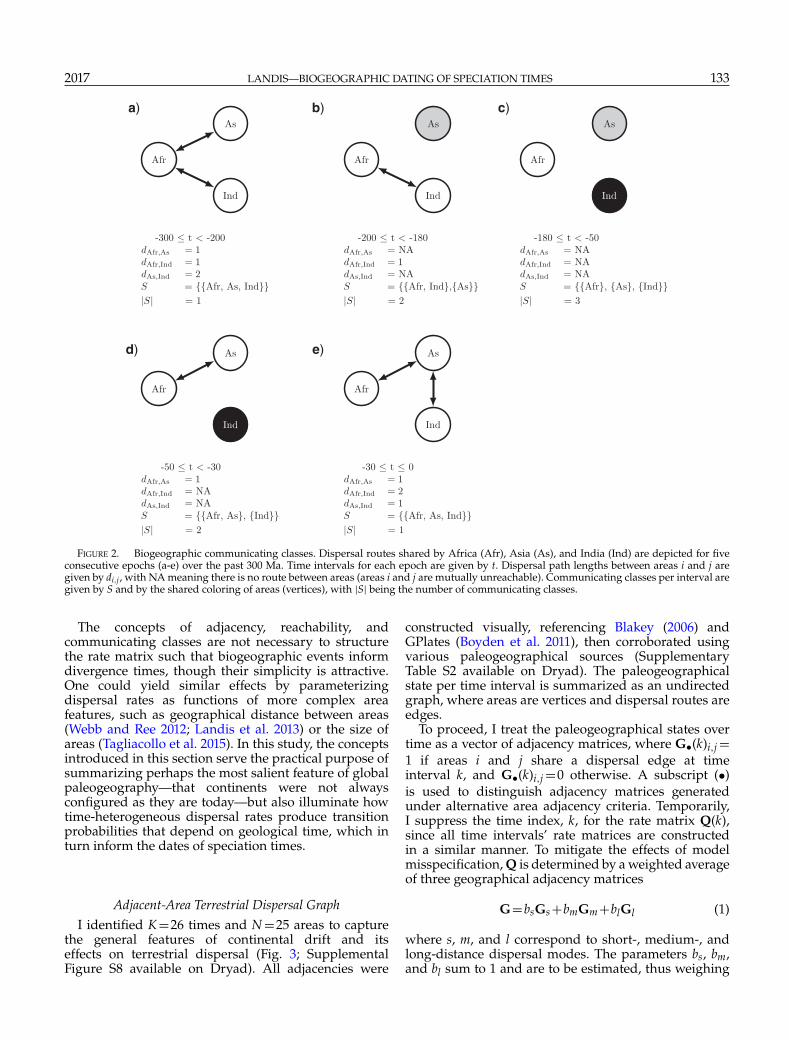
lineages are free to disperse between areas within thesepaleocontinents, but not to and from areas on otherpaleocontinents. For example, the set of communicatingclasses is S = {{Afr}, {As}, {Ind}} at t=−100, that is,there are |S|=3 communicating classes because no areasshare edges (Fig. 2c), while at t=−10 there is |S|=1communicating class since a path exists between all threepairs of areas (Fig. 2e).
In one extreme case, dispersals between mutuallyunreachable areas do not occur even after infinite time,and hence have zero probability. At the other extreme,when dispersal may occur between any pair of areaswith equal probability over all time intervals, thenpaleogeography does not favor nor disfavor dispersalevents (nor divergence events, implicitly) to occur duringparticular time intervals. In intermediate cases, wheredispersal probabilities between areas vary across timeintervals, the dispersal process informs when and whatdispersal (and divergence) events occur. For instance, thetransition probability of going from area i to j decreasesas the average path length between i and j increases.During some time intervals, the average path lengthbetween two areas might be short, thus dispersal eventsoccur more freely than when the average path is long.Comparing Figure 2a and e, the minimum numberof events required to disperse from India to Africa issmaller during the Triassic (e.g., at t=−250) than duringthe present (t=0), and thus would have a relativelyhigher probability given the process operated for thesame amount of time today (e.g., for a branch withthe same length). Interestingly, even lineages with nobiogeographic variation impart some information forwhen a period of biogeographic stasis might begin. Itwill be most probable for a lineage to remain in a givenarea during epochs where the area is not connectedto any dispersal routes. This particular signal of stasisis difficult, if not impossible, to account for underparsimony and node-based calibration methods.
Specifying communicating classes is partly difficultbecause we do not know the ease of dispersalbetween areas for most species throughout space andtime. Biologically, encoding zero-valued dispersal ratesdirectly into the model should be avoided giventhe apparent prevalence of long-distance dispersal,sweepstakes dispersal, etc. across dispersal barriers(Carlquist 1966). Mathematically, zero-valued rates mayimply that dispersal events between certain areas arenot merely improbable but utterly impossible, creatingtroughs of zero likelihood in the likelihood surfacefor certain dated-phylogeny-character patterns (Buerkiet al. 2011). In a biogeographic dating framework,this might unintentionally eliminate large numbersof speciation scenarios from the space of possiblehypotheses, resulting in distorted estimates. To avoidthese problems, I take the dispersal graph as theweighted average of three distinct dispersal graphsassuming short-, medium-, or long-distance dispersalmodes, each with their own set of communicatingclasses (see section “Adjacent-Area Terrestrial DispersalGraph”).
2017 LANDIS—BIOGEOGRAPHIC DATING OF SPECIATION TIMES 133
a) b) c)
d) e)
FIGURE 2. Biogeographic communicating classes. Dispersal routes shared by Africa (Afr), Asia (As), and India (Ind) are depicted for fiveconsecutive epochs (a-e) over the past 300 Ma. Time intervals for each epoch are given by t. Dispersal path lengths between areas i and j aregiven by di,j , with NA meaning there is no route between areas (areas i and j are mutually unreachable). Communicating classes per interval aregiven by S and by the shared coloring of areas (vertices), with |S| being the number of communicating classes.
The concepts of adjacency, reachability, andcommunicating classes are not necessary to structurethe rate matrix such that biogeographic events informdivergence times, though their simplicity is attractive.One could yield similar effects by parameterizingdispersal rates as functions of more complex areafeatures, such as geographical distance between areas(Webb and Ree 2012; Landis et al. 2013) or the size ofareas (Tagliacollo et al. 2015). In this study, the conceptsintroduced in this section serve the practical purpose ofsummarizing perhaps the most salient feature of globalpaleogeography—that continents were not alwaysconfigured as they are today—but also illuminate howtime-heterogeneous dispersal rates produce transitionprobabilities that depend on geological time, which inturn inform the dates of speciation times.
Adjacent-Area Terrestrial Dispersal GraphI identified K =26 times and N =25 areas to capture
the general features of continental drift and itseffects on terrestrial dispersal (Fig. 3; SupplementalFigure S8 available on Dryad). All adjacencies were
constructed visually, referencing Blakey (2006) andGPlates (Boyden et al. 2011), then corroborated usingvarious paleogeographical sources (SupplementaryTable S2 available on Dryad). The paleogeographicalstate per time interval is summarized as an undirectedgraph, where areas are vertices and dispersal routes areedges.
To proceed, I treat the paleogeographical states overtime as a vector of adjacency matrices, where G•(k)i,j =1 if areas i and j share a dispersal edge at timeinterval k, and G•(k)i,j =0 otherwise. A subscript (•)is used to distinguish adjacency matrices generatedunder alternative area adjacency criteria. Temporarily,I suppress the time index, k, for the rate matrix Q(k),since all time intervals’ rate matrices are constructedin a similar manner. To mitigate the effects of modelmisspecification, Q is determined by a weighted averageof three geographical adjacency matrices
G=bsGs +bmGm +blGl (1)
where s, m, and l correspond to short-, medium-, andlong-distance dispersal modes. The parameters bs, bm,and bl sum to 1 and are to be estimated, thus weighing

134 SYSTEMATIC BIOLOGY VOL. 66
N. America (NW)
N. America (SW)
N. America (NE)
Greenland
S. America (N)
S. America (E)
S. America (S)
Africa (W)
Africa (N)
Africa (E)
Africa (S)
Europe
Asia (C)
Asia (NE)
Asia (E)
Asia (SE)
MalaysianArchipelago
MadagascarIndia
Australia (SW)
Australia (NE)Antarctica (E)
Antarctica (W)
New Zealand
N. America (SE)
FIGURE 3. Dispersal graph for Epoch 14, 110–100Ma: India and Madagascar separate from Australia and Antarctica. A GPlates (Gurnis et al. 2012)screenshot of Epoch 14 of 26 is displayed. Areas are marked by black vertices. Black edges indicate both short- and medium-distance dispersalroutes. Gray edges indicate exclusively medium-distance dispersal routes. Long-distance dispersal routes are not shown, but are implied to existbetween all area-pairs. The short-, medium-, and long-distance dispersal graphs have 8, 1, and 1 communicating classes, respectively. Only Indiamay reach Madagascar by short-distance dispersal, and vice versa, forming one of the eight short-distance communicating classes. Both areasmaintain medium-distance dispersal routes with various Gondwanan continents during this epoch. The expansion of the Tethys Sea impedesdispersal into and out of Europe. Section “Paleogeography, Dispersal Graphs, and Markov Chains” explains how communicating classes aredetermined.
the importance of each dispersal mode according to thedata.
Short-, medium-, and long-distance dispersalprocesses encode strong, weak, and no geographicalconstraint, respectively. As distance-constrained modeweights bs and bm increase, the dispersal processgrows more prone to remaining within a particularcommunicating class (Supplementary Fig. S2 availableon Dryad). The vector of short-distance dispersal graphs,Gs = (Gs(1),Gs(2),...,Gs(K)), marks adjacencies for pairsof areas that allow terrestrial dispersal without travelingover bodies of water (Supplementary Figs. S2a,bavailable on Dryad ). Medium-distance dispersalgraphs, Gm, include all adjacencies in Gs in additionto adjacencies for areas separated by lesser bodies ofwater, such as throughout the Malay Archipelago,while excluding transoceanic adjacencies, such asbetween South America and Africa (SupplementaryFigs. S2c,d available on Dryad). Finally, long-distancedispersal graphs, Gl, allow dispersal events to occurbetween any pair of areas, regardless of potential barrier(Supplementary Figs. S2e,f available on Dryad).
To average over the three dispersal modes, bs, bm, andbl are constrained to sum to 1, causing all elements inG to take values from 0 to 1 (Equation 1). Importantly,adjacencies specified by Gs always equal 1, since thoseadjacencies are also found in Gm and Gl. This meansQ is a Jukes–Cantor rate matrix only when bl =1, but
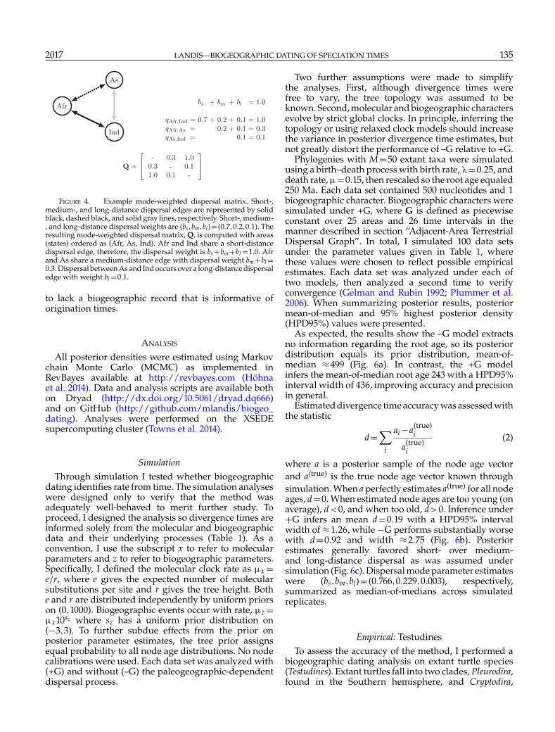
becomes increasingly paleogeographically structuredas bl →0. Non-diagonal elements of Q equal those ofG, but are rescaled such that the average number oftransitions per unit time is one, while diagonal elementsof Q equal the negative sum of the remaining rowelements. To compute transition probabilities, Q is laterrescaled by a biogeographic clock rate, �, prior to matrixexponentiation. The effects of the weights bs, bm, and blon dispersal rates between areas are shown in Figure 4.
By the argument that continental break-up (i.e., thecreation of new communicating classes; Figs. 1a,b)introduces a lower threshold on the minimum age ofdivergence, and that continental joining (i.e., unifyingexisting communicating classes; Figs. 1c,d) introducesan upper threshold on the maximum age of divergence,then the paleogeographical model I constructed hasthe greatest potential to provide both upper and lowerthresholds (soft bounds) on divergence times when thenumber of communicating classes is large, then small,then large again. This coincides with the formation ofPangaea, dropping from 8 to 3 communicating classesat 280 Ma, followed by the fragmentation of Pangaea,increasing from 3 to 11 communicating classes between170 Ma and 100 Ma (Fig. 5). It is important to considerthis bottleneck in the number of communicating classeswill be informative of root age only for fortuitouscombinations of species range and species phylogeny.Just as some clades lack a fossil record, others are bound
2017 LANDIS—BIOGEOGRAPHIC DATING OF SPECIATION TIMES 135
Q =
⎡⎣
- 0.3 1.00.3 - 0.11.0 0.1 -
⎤⎦
As
Ind
Afr bs + bm + bl = 1.0
qAfr,Ind = 0.7 + 0.2 + 0.1 = 1.0qAfr,As = 0.2 + 0.1 = 0.3qAs,Ind = 0.1 = 0.1
FIGURE 4. Example mode-weighted dispersal matrix. Short-,medium-, and long-distance dispersal edges are represented by solidblack, dashed black, and solid gray lines, respectively. Short-, medium-, and long-distance dispersal weights are (bs,bm,bl)= (0.7,0.2,0.1). Theresulting mode-weighted dispersal matrix, Q, is computed with areas(states) ordered as (Afr, As, Ind). Afr and Ind share a short-distancedispersal edge, therefore, the dispersal weight is bs +bm +bl =1.0. Afrand As share a medium-distance edge with dispersal weight bm +bl =0.3. Dispersal between As and Ind occurs over a long-distance dispersaledge with weight bl =0.1.
to lack a biogeographic record that is informative oforigination times.
ANALYSIS
All posterior densities were estimated using Markovchain Monte Carlo (MCMC) as implemented inRevBayes available at http://revbayes.com (Höhnaet al. 2014). Data and analysis scripts are available bothon Dryad (http://dx.doi.org/10.5061/dryad.dq666)and on GitHub (http://github.com/mlandis/biogeo_dating). Analyses were performed on the XSEDEsupercomputing cluster (Towns et al. 2014).
SimulationThrough simulation I tested whether biogeographic
dating identifies rate from time. The simulation analyseswere designed only to verify that the method wasadequately well-behaved to merit further study. Toproceed, I designed the analysis so divergence times areinformed solely from the molecular and biogeographicdata and their underlying processes (Table 1). As aconvention, I use the subscript x to refer to molecularparameters and z to refer to biogeographic parameters.Specifically, I defined the molecular clock rate as �x =e/r, where e gives the expected number of molecularsubstitutions per site and r gives the tree height. Bothe and r are distributed independently by uniform priorson (0,1000). Biogeographic events occur with rate, �z =�x10sz where sz has a uniform prior distribution on(−3,3). To further subdue effects from the prior onposterior parameter estimates, the tree prior assignsequal probability to all node age distributions. No nodecalibrations were used. Each data set was analyzed with(+G) and without (–G) the paleogeographic-dependentdispersal process.
Two further assumptions were made to simplifythe analyses. First, although divergence times werefree to vary, the tree topology was assumed to beknown. Second, molecular and biogeographic charactersevolve by strict global clocks. In principle, inferring thetopology or using relaxed clock models should increasethe variance in posterior divergence time estimates, butnot greatly distort the performance of –G relative to +G.
Phylogenies with M=50 extant taxa were simulatedusing a birth–death process with birth rate, �=0.25, anddeath rate, �=0.15, then rescaled so the root age equaled250 Ma. Each data set contained 500 nucleotides and 1biogeographic character. Biogeographic characters weresimulated under +G, where G is defined as piecewiseconstant over 25 areas and 26 time intervals in themanner described in section “Adjacent-Area TerrestrialDispersal Graph”. In total, I simulated 100 data setsunder the parameter values given in Table 1, wherethese values were chosen to reflect possible empiricalestimates. Each data set was analyzed under each oftwo models, then analyzed a second time to verifyconvergence (Gelman and Rubin 1992; Plummer et al.2006). When summarizing posterior results, posteriormean-of-median and 95% highest posterior density(HPD95%) values were presented.
As expected, the results show the –G model extractsno information regarding the root age, so its posteriordistribution equals its prior distribution, mean-of-median ≈499 (Fig. 6a). In contrast, the +G modelinfers the mean-of-median root age 243 with a HPD95%interval width of 436, improving accuracy and precisionin general.
Estimated divergence time accuracy was assessed withthe statistic
d=∑
i
ai −a(true)i
a(true)i
(2)
where a is a posterior sample of the node age vectorand a(true) is the true node age vector known throughsimulation. When a perfectly estimates a(true) for all nodeages, d=0. When estimated node ages are too young (onaverage), d<0, and when too old, d>0. Inference under+G infers an mean d=0.19 with a HPD95% intervalwidth of ≈1.26, while −G performs substantially worsewith d=0.92 and width ≈2.75 (Fig. 6b). Posteriorestimates generally favored short- over medium-and long-distance dispersal as was assumed undersimulation (Fig. 6c). Dispersal mode parameter estimateswere (bs,bm,bl)= (0.766,0.229,0.003), respectively,summarized as median-of-medians across simulatedreplicates.
Empirical: TestudinesTo assess the accuracy of the method, I performed a
biogeographic dating analysis on extant turtle species(Testudines). Extant turtles fall into two clades, Pleurodira,found in the Southern hemisphere, and Cryptodira,

136 SYSTEMATIC BIOLOGY VOL. 66
500 400 300 200 100 0
com
m. c
lass
es (s
hort)
500 400 300 200 100 0
com
m. c
lass
es (m
ed.)
500 400 300 200 100 0age
# co
mm
. cla
sses
13
57
911 short med. long
a)
b)
c)
FIGURE 5. Dispersal graph properties summarized over time. Communicating classes of the short-distance dispersal graph (a) and medium-distance dispersal graph (b) are shown. Each of 25 areas is represented by one horizontal line. Colors of areas (online figure only) match thoselisted in Supplementary Figure S2 (available on Dryad). On the vertical axis, areas that share a communicating class are grouped into horizontalbands (multiple lines) whose width is proportional to the number of areas in the communicating class. Vertical lines running between horizontalbands indicate transitions of areas joining or leaving communicating classes, that is, due to paleogeographical events. Communicating classesare arranged vertically to appear horizontally stable with respect to time, but their vertical order and relative positioning is otherwise arbitrary.When no transition event occurs for an area entering a new epoch, the line is interrupted with a gap. The two arrows mark the break-up ofWest Gondwana, first recorded in the short-distance dispersal graph (a) at 120 Ma, then later in the medium-distance dispersal graph (b) at 90Ma. c) Number of communicating classes: the black line corresponds to the short-distance dispersal graph (a), the dotted line corresponds tomedium-distance dispersal graph (b), and the gray line corresponds to the long-distance dispersal graph, which always has one communicatingclass. Section “Paleogeography, Dispersal Graphs, and Markov Chains” explains how communicating classes are determined.
found predominantly in the Northern hemisphere.Their modern distribution shadows their biogeographichistory, where Testudines is thought to be Gondwananin origin with the ancestor to cryptodires dispersinginto Laurasia during the Jurassic (Crawford et al. 2015).Since turtles are among the best preserved vertebrates inthe fossil record, their phylogeny and divergence timeshave been profitably analyzed and reanalyzed by variousresearchers (Hugall et al. 2007; Joyce 2007; Danilov andParham 2008; Alfaro et al. 2009; Dornburg et al. 2011;Joyce et al. 2013; Sterli et al. 2013; Warnock et al. 2015). Thismakes them ideal to assess the efficacy of biogeographicdating, which makes no use of their replete fossil record:if both biogeography-based and fossil-based methodsgenerate similar results, they co-validate each others’
correctness (assuming they are not both biased in thesame manner).
To proceed, I assembled a moderately sized dataset.First, I aligned cytochrome B sequences for 185 turtlespecies (155 cryptodires, 30 pleurodires) using MUSCLE3.8.31 (Edgar 2004) under the default settings. Assumingthe 25-area model presented in section “Adjacent-AreaTerrestrial Dispersal Graph”, I consulted GBIF (gbif.org)and IUCN Red List (iucnredlist.org) to record the area(s)in which each species was found. Species occupyingmultiple areas were assigned ambiguous tip statesfor those areas. Missing data entries were assignedto the six sea turtle species used in this study toeffectively eliminate their influence on the (terrestrial)biogeographic process. To simplify the analysis, I

2017 LANDIS—BIOGEOGRAPHIC DATING OF SPECIATION TIMES 137
TABLE 1. Model parameters
Parameter X Simulation f (X) sim. value Empirical f (X)
Tree Root age r Uniform(0,1000) 250 Uniform(0,540) orUniform(155.7,251.4)
Time tree � UniformTimeTree(r) BD(�=0.25,�=0.15) UniformTimeTree(r)Molecular Length e Uniform(0,1000) 2.5 Uniform(0,1000)
Subst. rate �x e/r Determined (0.01) e/rExch. rates rx Dirichlet(10) From prior Dirichlet(1)Stat. freqs �x Dirichlet(10) From prior Dirichlet(1)Rate matrix Qx GTR(rx,�x) Determined GTR(rx,�x)Branch rate mult. �x,i Lognorm(ln�x −�2
x/2,�x)Branch rate var. �x Exponential(0.1)+4 x Gamma(,)+4 hyperprior Uniform(0,50)
Biogeo. Atlas-graph G(t) –G or +G +G +GBiogeo. rate �z �x10sz Determined (0.1) �x10sz
Biogeo. rate mod. sz Uniform(-3, 3) 1.0 Uniform(-3, 3)Dispersal mode (bs,bm,bl) Dirichlet(1) (1000,10,1)/1011 Dirichlet(1,1,1) or
Dirichlet(100,10,1)Dispersal rates rz(t)
∑i∈{s,m,l}biGi(t) Determined
∑i∈{s,m,l}biGi(t)
Stat. freqs �z (1,...,1)/25 (1,...,1)/25 (1,...,1)/25Rate matrix Qz(t) GTR(rz(t),�z) Determined GTR(rz(t),�z)
Notes: Model parameter names and prior distributions are described in the manuscript body. All empirical priors were identical to simulatedpriors unless otherwise stated. Priors used for the empirical analyses but not simulated analyses are left blank. Determined means the parametervalue was determined by other model parameters.
a) b) c)
FIGURE 6. Posterior estimates for simulated data. a) Posterior estimates of root age. The true root age for all simulations is 250 Ma (dottedvertical line). b) Posterior estimates of relative node age error (Equation 2). The true error term equals zero. Both a and b) paleogeographicallynon-informed (–G) analyses are on the top half, and paleogeographically informed (+G) analyses are on the bottom. Each square marks theposterior mean root age estimate with the HPD95% credible interval. Estimates whose credible interval did not contain the true value aredarkened for visibility. c) Posterior estimates of dispersal mode proportions for the +G simulations projected onto the unit 2-simplex. The filledsquare (near “short”) gives the true value, and the empty circles give posterior medians.
138 SYSTEMATIC BIOLOGY VOL. 66
0 100 200 300 400 500
0.00
00.
004
0.00
80.
012
root age
Den
sity
(roo
t age
)Uniform(0, 540), +G, flatUniform(0, 540), +G, shortUniform(0, 540), GUniform(156, 251), +G, flatUniform(156, 251), +G, shortUniform(156, 251), G
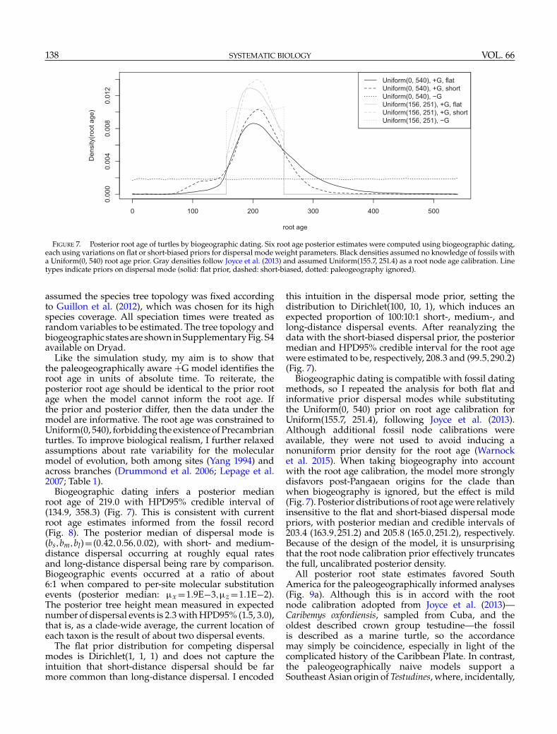
FIGURE 7. Posterior root age of turtles by biogeographic dating. Six root age posterior estimates were computed using biogeographic dating,each using variations on flat or short-biased priors for dispersal mode weight parameters. Black densities assumed no knowledge of fossils witha Uniform(0, 540) root age prior. Gray densities follow Joyce et al. (2013) and assumed Uniform(155.7, 251.4) as a root node age calibration. Linetypes indicate priors on dispersal mode (solid: flat prior, dashed: short-biased, dotted: paleogeography ignored).
assumed the species tree topology was fixed accordingto Guillon et al. (2012), which was chosen for its highspecies coverage. All speciation times were treated asrandom variables to be estimated. The tree topology andbiogeographic states are shown in Supplementary Fig. S4available on Dryad.
Like the simulation study, my aim is to show thatthe paleogeographically aware +G model identifies theroot age in units of absolute time. To reiterate, theposterior root age should be identical to the prior rootage when the model cannot inform the root age. Ifthe prior and posterior differ, then the data under themodel are informative. The root age was constrained toUniform(0, 540), forbidding the existence of Precambrianturtles. To improve biological realism, I further relaxedassumptions about rate variability for the molecularmodel of evolution, both among sites (Yang 1994) andacross branches (Drummond et al. 2006; Lepage et al.2007; Table 1).
Biogeographic dating infers a posterior medianroot age of 219.0 with HPD95% credible interval of(134.9, 358.3) (Fig. 7). This is consistent with currentroot age estimates informed from the fossil record(Fig. 8). The posterior median of dispersal mode is(bs,bm,bl)= (0.42,0.56,0.02), with short- and medium-distance dispersal occurring at roughly equal ratesand long-distance dispersal being rare by comparison.Biogeographic events occurred at a ratio of about6:1 when compared to per-site molecular substitutionevents (posterior median: �x =1.9E−3,�z =1.1E−2).The posterior tree height mean measured in expectednumber of dispersal events is 2.3 with HPD95% (1.5, 3.0),that is, as a clade-wide average, the current location ofeach taxon is the result of about two dispersal events.
The flat prior distribution for competing dispersalmodes is Dirichlet(1, 1, 1) and does not capture theintuition that short-distance dispersal should be farmore common than long-distance dispersal. I encoded
this intuition in the dispersal mode prior, setting thedistribution to Dirichlet(100, 10, 1), which induces anexpected proportion of 100:10:1 short-, medium-, andlong-distance dispersal events. After reanalyzing thedata with the short-biased dispersal prior, the posteriormedian and HPD95% credible interval for the root agewere estimated to be, respectively, 208.3 and (99.5,290.2)(Fig. 7).
Biogeographic dating is compatible with fossil datingmethods, so I repeated the analysis for both flat andinformative prior dispersal modes while substitutingthe Uniform(0, 540) prior on root age calibration forUniform(155.7, 251.4), following Joyce et al. (2013).Although additional fossil node calibrations wereavailable, they were not used to avoid inducing anonuniform prior density for the root age (Warnocket al. 2015). When taking biogeography into accountwith the root age calibration, the model more stronglydisfavors post-Pangaean origins for the clade thanwhen biogeography is ignored, but the effect is mild(Fig. 7). Posterior distributions of root age were relativelyinsensitive to the flat and short-biased dispersal modepriors, with posterior median and credible intervals of203.4 (163.9,251.2) and 205.8 (165.0,251.2), respectively.Because of the design of the model, it is unsurprisingthat the root node calibration prior effectively truncatesthe full, uncalibrated posterior density.
All posterior root state estimates favored SouthAmerica for the paleogeographically informed analyses(Fig. 9a). Although this is in accord with the rootnode calibration adopted from Joyce et al. (2013)—Caribemys oxfordiensis, sampled from Cuba, and theoldest described crown group testudine—the fossilis described as a marine turtle, so the accordancemay simply be coincidence, especially in light of thecomplicated history of the Caribbean Plate. In contrast,the paleogeographically naive models support aSoutheast Asian origin of Testudines, where, incidentally,

2017 LANDIS—BIOGEOGRAPHIC DATING OF SPECIATION TIMES 139
0
200
400
Uni
form
(0, 5
40),
G
Uni
form
(0, 5
40),
+G, f
lat
Uni
form
(0, 5
40),
+G, s
hort
Uni
form
(156
, 251
), G
Uni
form
(156
, 251
), +G
, fla
t
Uni
form
(156
, 251
), +G
, sho
rt
Joyc
e 07
Ste
rli e
t al 1
3
Dan
ilov
& P
arha
m 0
8
(nt)
Hug
all e
t al 0
7
(*) W
arno
ck e
t al 1
5
Joyc
e et
al 1
3
(aa)
Hug
all e
t al 0
7
Alfa
ro e
t al 0
9
Dor
nbur
g et
al 1
1
Model or study
Roo
t age
est
imat
es
FIGURE 8. Root age comparison. Root age estimates are presented both for analysis conducted for this manuscript and as reported in theliterature. Existing estimates are as reported in Sterli et al. (2013) and supplemented recently reported results. Points and whiskers correspondto the point estimates their confidence intervals. The six left estimates were computed using biogeographic dating, each using variations on flator short-biased priors for key parameters. Two of these analyses ignore paleogeography (–G) so the posterior root age is the uniform prior rootage, whose mode (not shown) equals all values supported by the prior. Hugall et al. (2007) report ages for analyses using amino acids (aa) andnucleotides (nt). Warnock et al. (2015) report many estimates while exploring prior sensitivity, but only uniform prior results are shown here.
Southeast Asia is the most frequently inhabited areaamong the 185 testudines. For the analysis with a flatdispersal mode prior and no root age calibration, allroot states with high posterior probability appear toconcur upon the posterior root age density (Fig. 9b),that is, regardless of conditioning on the northernarea of South America or either of the two southernareas in North America as a root state, the posteriorroot age density is roughly equal. Similarly, poorlysupported areas of origin contribute almost nothing tothe root age density. The joint-marginal density sharedby the root age and root state variables bears a strongsignature of a unimodality, for example, young and oldorigination times do not support conflicting areas oforigin. Ancestral biogeographic state estimates for theentire clade are available as Supplementary Figs. S5–S7.
DISCUSSION
A major obstacle preventing the probabilistic unionof paleogeographical knowledge, biogeographicinference, and divergence time estimation has beenmethodological, which I have attempted to redressin this article. The intuition justifying prior-basedfossil calibrations (Parham et al. 2012), that is, thatfossil occurrences should somehow inform divergencetimes, has recently been formalized into several models(Pyron 2011; Ronquist et al. 2012; Heath et al. 2014).Here, I present an analogous treatment for prior-basedbiogeographic calibrations, that is, that biogeographicpatterns of modern species echo time-calibratedpaleobiogeographic events, by describing how epochmodels (Ree et al. 2005; Ree and Smith 2008; Bielejec

140 SYSTEMATIC BIOLOGY VOL. 66
Prob(area)P
rob(
root
age
)
020406080
100120140160180200220240260280300320340360380400420440460480500520
S. A
mer
ica
(N)
S. A
mer
ica
(E)
S. A
mer
ica
(S)
N. A
mer
ica
(NW
)N
. Am
eric
a (S
E)
N. A
mer
ica
(NE
)N
. Am
eric
a (S
W)
Gre
enla
ndE
urop
eA
sia
(C)
Asi
a (E
)A
sia
(SE
)A
sia
(NE
)A
frica
(W)
Afri
ca (S
)A
frica
(E)
Afri
ca (N
)A
ustra
lia (N
)A
ustra
lia (S
)In
dia
Mad
agas
car
Ant
arct
ica
(W)
Ant
arct
ica
(E)
Mal
aysi
an A
rch.
New
Zea
land
0.00
0.02
0.04
0.06
0.08
0.10
0.12
0.14
0.16
Prob(area)
Mod
el o
r dat
a
Unif(151, 251), +G, shortUnif(151, 251), +G, flat Unif(151, 251), G
Unif(0, 540), +G, shortUnif(0, 540), +G, flat Unif(0, 540), G
Tip state frequencies
S. A
mer
ica
(N)
S. A
mer
ica
(E)
S. A
mer
ica
(S)
N. A
mer
ica
(NW
)N
. Am
eric
a (S
E)
N. A
mer
ica
(NE
)N
. Am
eric
a (S
W)
Gre
enla
ndE
urop
eA
sia
(C)
Asi
a (E
)A
sia
(SE
)A
sia
(NE
)A
frica
(W)
Afri
ca (S
)A
frica
(E)
Afri
ca (N
)A
ustra
lia (N
)A
ustra
lia (S
)In
dia
Mad
agas
car
Ant
arct
ica
(W)
Ant
arct
ica
(E)
Mal
aysi
an A
rch.
New
Zea
land
0.0
0.2
0.4
0.6
0.8
1.0
b)a)
FIGURE 9. Root state estimates. a) Posterior probabilities of root state are given for the six empirical analyses. b) Joint-marginal posteriorprobabilities of root age and root state are given for the empirical analysis without a root calibration and with a flat dispersal mode prior. Rootages are binned into intervals of width 20.
et al. 2014) are informative of absolute divergencetimes. Briefly, I accomplished this using a simpletime-heterogeneous dispersal process (Sanmartín et al.2008), where dispersal rates are piecewise constant, anddetermined by a graph-based paleogeographical model(section “Adjacent-Area Terrestrial Dispersal Graph”).The paleogeographical model itself was constructedby translating various published paleogeographicalreconstructions (Supplementary Table S2 available onDryad) into a time-calibrated vector of dispersal graphs(Fig. 3 and Supplementary Fig. S8 available on Dryad).Because area adjacencies are abiotic paleogeographicalfeatures, and because the biogeographic model estimateshow severely paleogeographic adjacency constrainsspecies dispersal, the model is generally appropriate foruse with other terrestrial clades.
Through simulation, I showed that biogeographicdating identifies clade age from the rates of molecularand biogeographic character change. Following that,the simulation framework could easily be extendedto investigate for what phylogenetic, paleogeographic,and biogeographic conditions one is able to reliablyextract information for the root age. For example,a clade with taxa invariant for some biogeographicstate would contain little to no information about rootage, provided the area has always existed and hada constant number of dispersal edges over time. Atthe other extreme, a clade with a very high dispersalrate or with a proclivity toward long-distance dispersalmight provide little information due to signal saturation(Supplementary Figs. S2e,f available on Dryad). Thebreadth of applicability of biogeographic dating willdepend critically on such factors, but because we do
not expect to see closely related species uniformlydistributed about Earth nor in complete sympatry, thatbreadth may not be so narrow.
After validating the method through simulation, Itested whether divergence times might be estimatedfrom extant taxa in an empirical system, Testudines.I assumed a flat root age calibration prior for theorigin time of turtles: the posterior root age wasalso flat when paleogeography was ignored, butPangaean times of origin were strongly preferredwhen dispersal rates conditioned on paleogeography(Fig. 7). Under the uninformative prior distributionson root age, biogeographic dating estimated turtlesoriginated between the Late Devonian (358 Ma) andEarly Cretaceous (135 Ma) epochs, with a posteriormedian age of 219 Ma. Under an ignorance prior whereshort-, medium-, and long-distance dispersal eventshave equal prior rates, short- and medium-distancedispersal modes are strongly favored over long-distancedispersal. Posterior estimates changed little by informingthe prior to strongly prefer short-distance dispersal. Bothwith and without root age calibrations, and with both flatand informative dispersal mode priors, biogeographicdating placed the posterior median origin time of turtlesat approximately 220–200 Ma, which is consistent withfossil-based estimates (Fig. 8), albeit with less precision.
The increased uncertainty in the root age estimatesunder biogeographic dating may be caused by anycombination of possible factors. First, in the absenceof fossils, biogeographic events are historical andnot observed directly. Through inference, all possiblebiogeographic scenarios are assigned plausibilityin terms of their likelihoods, which inherently

2017 LANDIS—BIOGEOGRAPHIC DATING OF SPECIATION TIMES 141
introduces uncertainty that any one history occurred. Bycomparison, turtle fossils can be placed with relativelyhigh phylogenetic and temporal certainty, and thusproduce more precise estimates. Second, the model andpriors are designed to contrast how well biogeographicdating (+G) estimates divergence times relative toa state of complete geographical ignorance (−G).For example, using a time-homogeneous birth–deathprocess prior will cause divergence events to followa more clock-like pattern, which is likely to be morerealistic than a uniform time tree prior, which has highnode age variance by design. Additional fossil nodecalibrations were available for use from Joyce et al.(2013), but they induce a non-uniform root age priordistribution (Warnock et al. 2015), and would havecomplicated the interpretation of the results. Betterbehaved priors are available and recommended forrigorous empirical investigations. Third, limited by theavailability of genetic data, only 185 of over 300 extanttestudines were used in the analysis. Increased taxonsampling generally improves ancestral state estimation(Heath et al. 2008), which will translate to improvednode age estimation for biogeographic dating. Fourth,process-based dating methods are sensitive to theunderlying model assumptions (O’Reilly et al. 2015),and, in the section to come, I explore how modelinadequacies might affect biogeographic dating.
Nonetheless, biogeographic dating generatesrelatively uncertain root age estimates when comparedto previously published fossil-based results on aper-study basis. The nine fossil-based estimates wereproduced using diverse techniques (Figure 8): fourwere estimated with node-dating (Warnock et al. 2015;Alfaro et al. 2009; Joyce et al. 2013; Dornburg et al.2011), three with maximum parsimony (Sterli et al. 2013;Joyce 2007; Danilov and Parham 2008), and two withpenalized likelihood rate smoothing (Hugall et al. 2007;nucleotides and amino acids). Among these studies,the average support interval width is approximately45 Ma while their combined supported root ages areover three times as wide, ranging from 145 Ma at theyoungest to 324 Ma at the oldest (width 179 Ma). Onthis note, at least three of the nine fossil-based root ageestimates must be incorrect due to the poor supportinterval overlap. For dating exercises, it is worth notingthat precision should not be maximized for its own sake.Uncertainty is valuable when it is correctly measuredand guards against being positively incorrect. That said,the combined fossil-based support interval (145 Ma to324 Ma) is still 31% narrower than the supported agesreported across the biogeographic dating analyses (100Ma to 358 Ma, width 258 Ma, excluding –G analyses).
Exercises comparing performance between fossil-based and biogeographic-based dating are left for futurework. However, fossil-based and biogeography-baseddating methods should not be viewed as competitive,since nothing inherently prevents them from beingapplied simultaneously to further improve precision. Forexample, under the design of the earlier biogeographicdating analysis, adding a root age prior effectively
truncates the posterior density (Figure 7), thus allowingfossil-based hypotheses to tune the precision of root ageestimates.
For groups with poor fossil records, biogeographicdating provides a second hope for dating divergencetimes. Since biogeographic dating does not rely onany fossilization process or data directly, it is readilycompatible with existing fossil-based dating methods(Figure 7). When fossils with geographic information areavailable, researchers have shown fossil taxa improvebiogeographic inferences (Moore et al. 2008; Maoet al. 2012; Nauheimer et al. 2012; Wood et al. 2012;Meseguer et al. 2015). In principle, the processes ofmorphological and biogeographic evolution shouldguide placement of fossils on the phylogeny, and theage of the fossils should improve the certainty inestimates of ancestral biogeographic states (Slater et al.2012), on which biogeographic dating relies. A jointtip-dated and biogeography-dated analysis under thefossilized birth–death process (Gavryushkina et al. 2015;Zhang et al. 2015) would produce improved node ageestimates in a methodologically consistent framework.Joint inference of divergence times, biogeography, andfossilization stands to resolve recent paleobiogeographicconundrums that may arise when considering inferencesseparately (Beaulieu et al. 2013; Wilf and Escapa 2014).
Model Inadequacies and Future ExtensionsThe simulated and empirical studies demonstrate
biogeographic dating improves divergence timeestimates, with and without fossil calibrations, but manyshortcomings in the model remain to be addressed.When any model is misspecified, inference is expected toproduce uncertain or, worse, spurious results (Lemmonand Moriarty 2004), and biogeographic models are notexempted. Because the biogeographic model assumedin the analysis is so very simple, a rigorous battery ofsimulation studies must be carried out to assess themethod’s robustness when faced with model violation.To this end, I discuss some of the most apparent modelmisspecifications below.
Anagenetic range evolution models that properlyallow species to inhabit multiple areas should improvethe informativeness of biogeographic data. Imagine taxaT1 and T2 inhabit areas ABCDE and FGHIJ, respectively.Under the simple model assumed in this article, thetip states are ambiguous with respect to their ranges,and for each ambiguous state only a single dispersalevent is needed to reconcile their ranges. Under a pureanagenetic range evolution model (Ree et al. 2005), atleast five dispersal events are needed for reconciliation.Additionally, some extant taxon ranges may span ancientbarriers, such as a terrestrial species found both northand south of the Isthmus of Panama. When multiple-area ranges are used, this situation almost certainlyrequires a dispersal event to have occurred after theisthmus was formed. For single-area species rangescoded as ambiguous states, the model effectively takes

142 SYSTEMATIC BIOLOGY VOL. 66
the weighted average of the lineage being only north andbeing only south of the isthmus, so information aboutthe effects of the paleogeographical event on divergencetimes will be relatively diluted.
Any model where the diversification processand paleogeographical states (and events) arecorrelated or co-occuring will obviously improvedivergence time estimates so long as that relationshipis biogeographically realistic. Although the repertoireof cladogenetic models is expanding in terms oftypes of transition events, they do not yet account forgeographical features, such as continental adjacency orgeographical distance. Incorporating paleogeographicalstructure into cladogenetic models of geographicallyisolated speciation, such as vicariance (Ronquist 1997),allopatric speciation (Ree et al. 2005; Goldberg et al.2011), and jump dispersal (Matzke 2014), is crucialnot only to generate information for biogeographicdating analyses, but also to improve the accuracy ofancestral range estimates. Ultimately, cladogeneticevents are state-dependent speciation events, so thedesired process would model range evolution jointlywith the birth–death process (Maddison et al. 2007;Goldberg et al. 2011), but inference under thesemodels for large state spaces is currently infeasible.Regardless, any cladogenetic range-division eventrequires a widespread range, which in turn implies itwas preceded by dispersal (range expansion) events.Thus, if we accept that paleogeography constrains thedispersal process, even a simple dispersal-only modelwill extract dating information when describing a farmore complex evolutionary process.
That said, the simple paleogeographical modeldescribed herein (section “Adjacent-Area TerrestrialDispersal Graph”) has many shortcomings itself. It isonly designed for terrestrial species originating in thelast 540 Ma. The number of epochs and areas waslimited by my ability to comb the literature for well-supported paleogeological events, while constrainedby computational considerations (see SupplementaryMaterial available on Dryad). The timing of events wasassumed to be known perfectly, despite the literaturereporting ranges of estimates. Rates of dispersal betweenareas are classified into short, medium, and longdistances, but using necessarily practical and subjectivecriteria. Factors such as temperature, precipitation,ocean currents, ecoregion type, distances betweenareas, sizes of areas, carrying capacities, etc. certainlyaffect dispersal rates between areas in terms ofmagnitude and symmetry, and in terms of the stationaryfrequencies per epoch, but were ignored. These factorsmay be integrated into the existing paleogeographicalmodel so long as the data are available. Fromthe modeling perspective, the rate matrix equation(Equation 1) can accommodate additional layers ofhistorical features, such as those listed above, throughadditional weight parameters and rate matrix vectors.Regarding how to incorporate those features, Sanmartínet al. (2008) suggest how the biogeographic rate matrixmay encode various celebrated colonization models
(MacArthur and Wilson 1967; Hanski 1994). Finally,these colonization rates are likely to interact with theevolving life history traits intrinsic to each lineage,such as flightedness or cold tolerance, as modeled bySukumaran et al. (2015). All of these factors can andshould be handled more rigorously in future studies bymodeling these processes and factors as part of a jointBayesian analysis (Höhna et al. 2014).
Despite these flaws, defining the paleogeographicalmodel serves as an exercise to identify what featuresallow a biogeographic process to inform speciationtimes. Identifying significant areas and epochs remainschallenging, where presumably more areas and epochsare better to approximate continuous space and time,but this is not without computational challenges(Ree and Sanmartín 2009; Webb and Ree 2012; Landiset al. 2013). Dispersal barriers are clearly clade-dependent and depend on various life history traits,for example, benthic marine species dispersal wouldbe poorly modeled by the terrestrial graph. Classifyingdispersal edges into dispersal mode classes may bemade rigorous using clustering algorithms informedby paleogeographical features, or even abandonedin favor of modeling rates directly as functions ofpaleogeographical features like distance. Rather thanfixing epoch event times to point estimates, one mightassign empirical prior distributions based on collectedestimates. Ideally, paleogeographical event times andfeatures would be estimated jointly with phylogeneticevidence, which would require interfacing phylogeneticinference with paleogeographical inference. FollowingSanmartín et al. (2008), multi-clade biogeographicanalyses could be used to generate the statisticalpower necessary to obtain reliable paleogeographicalestimates. This would be a profitable, but substantial,interdisciplinary undertaking.
ConclusionHistorical biogeography is undergoing a probabilistic
renaissance, owing to the abundance of georeferencedbiodiversity data now hosted online and the explosionof newly published biogeographic models and methods(Ree et al. 2005; Ree and Smith 2008; Sanmartín et al.2008; Lemmon and Lemmon 2008; Lemey et al. 2010;Goldberg et al. 2011; Webb and Ree 2012; Landis et al.2013; Matzke 2014; Sukumaran et al. 2015; Tagliacolloet al. 2015). Making use of these advances, I have shownhow patterns latent in biogeographic characters, whenviewed with a paleogeographic perspective, provideinformation about the geological timing of speciationevents. The method conditions directly on biogeographicobservations to induce dated node age distributions,rather than imposing (potentially incorrect) beliefs aboutspeciation times using node calibration densities, whichare data-independent prior densities. Biogeographicdating may present new opportunities for datingphylogenies for fossil-poor clades since the techniquerequires no fossils. This establishes that historical
2017 LANDIS—BIOGEOGRAPHIC DATING OF SPECIATION TIMES 143
biogeography has untapped practical use for statisticalphylogenetic inference, and should not be considered ofsecondary interest, only to be analyzed after the speciestree is estimated.
SUPPLEMENTARY MATERIAL
Data available from the Dryad Digital Repository:http://dx.doi.org/10.5061/dryad.dq666.
FUNDING
This work was supported by a National EvolutionarySynthesis Center Graduate Fellowship to M.J.L. anda National Institutes of Health [grant R01-GM069801]awarded to John P. Huelsenbeck. Simulation analyseswere computed using XSEDE, which is supportedby National Science Foundation [grant number ACI-1053575].
ACKNOWLEDGMENTS
I thank Tracy Heath, Sebastian Höhna, Josh Schraiber,Lucy Chang, Pat Holroyd, Nick Matzke, MichaelDonoghue, and John Huelsenbeck for valuable feedback,support, and encouragement regarding this work. I givemy special thanks to James Albert, Alexandre Antonelli,and the Society of Systematic Biologists for inviting meto present this research at Evolution 2015 in Guarujá,Brazil. Frank Anderson, Emma Goldberg, and threeanonymous reviewers provided feedback that greatlyimproved the clarity of the manuscript.
REFERENCES
Alfaro M.E., Santini F., Brock C., Alamillo H., Dornburg A., RaboskyD.L., Carnevale G., Harmon L.J. 2009. Nine exceptional radiationsplus high turnover explain species diversity in jawed vertebrates.Proc. Natl Acad. Sci. 106:13410–13414.
Beaulieu J.M., Tank D.C., Donoghue M.J. 2013. A Southern Hemisphereorigin for campanulid angiosperms, with traces of the break-up ofGondwana. BMC Evol. Biol. 13:80.
Behrensmeyer A.K., Kidwell S.M., Gastaldo R.A. 2000. Taphonomy andpaleobiology. Paleobiology 26:103–147.
Bielejec F., Lemey P., Baele G., Rambaut A., Suchard M.A. 2014.Inferring heterogeneous evolutionary processes through time: fromsequence substitution to phylogeography. Syst. Biol. 63:493–504.
Blakey R. 2008. Global paleogeographic views of Earth history–LatePrecambrian to Recent. Colorado Plateau Geosystems, Inc. URL:http://cpgeosystems.com/paleomaps.html.
Boyden J.A., Müller R.D., Gurnis M., Torsvik T.H., Clark J.A., TurnerM., Ivey-Law H., Watson R.J., Cannon J.S. 2011. Next-generationplate-tectonic reconstructions using GPlates. In: Keller G. R., editor.Geoinformatics: cyberinfrastructure for the solid earth sciences.New York: Cambridge University Press, p. 95–114.
Buerki S., Forest F., Alvarez N., Nylander J.A.A., Arrigo N., SanmartínI. 2011. An evaluation of new parsimony-based versus parametricinference methods in biogeography: a case study using the globallydistributed plant family Sapindaceae. J. Biogeog. 38:531–550.
Carlquist S. 1966. The biota of long-distance dispersal. I. Principles ofdispersal and evolution. Q. Rev. Biol. 41:247–270.
Crawford N.G., Parham J.F., Sellas A.B., Faircloth B.C., Glenn T.C.,Papenfuss T.J., Henderson J.B., Hansen M.H., Simison B.W. 2015.A phylogenomic analysis of turtles. Mol. Phylogen. Evol. 83:250–257.
Danilov I.G., Parham J.F. 2008. A reassessment of some poorly knownturtles from the Middle Jurassic of China, with comments on theantiquity of extant turtles. J. Vert. Paleontol. 28:306–318.
Dornburg A., Beaulieu J.M., Oliver J.C., Near T.J. 2011. Integrating fossilpreservation biases in the selection of calibrations for moleculardivergence time estimation. Syst. Biol. 60:519–527.
Drummond A.J., Ho S.Y., Phillips M.J., Rambaut A. 2006. Relaxedphylogenetics and dating with confidence. PLoS Biol. 4:e88.
Edgar R.C. 2004. MUSCLE: Multiple sequence alignment with highaccuracy and high throughput. Nucleic Acids Res. 32:1792–1797.
Felsenstein J. 1981. Evolutionary trees from DNA sequences: Amaximum likelihood approach. J. Mol. Evol. 17:368–376.
Gavryushkina A., Heath T.A., Ksepka D.T., Stadler T., Welch D.,Drummond A.J. 2015. Bayesian total evidence dating reveals therecent crown radiation of penguins. arXiv preprint arXiv:1506.04797.
Gelman A., Rubin D.B. 1992. Inferences from iterative simulation usingmultiple sequences. Stat. Sci. 7:457–511.
Goldberg E.E., Lancaster L.T., Ree R.H. 2011. Phylogenetic inferenceof reciprocal effects between geographic range evolution anddiversification. Syst. Biol. 60:451–465.
Guillon J.-M., Guéry L., Hulin V., Girondot M. 2012. A large phylogenyof turtles (Testudines) using molecular data. Cont. Zool. 81:147–158.
Gurnis M., Turner M., Zahirovic S., DiCaprio L., Spasojevic S., MüllerR.D., Boyden J., Seton M., Manea V.C., Bower D.J. 2012. Plate tectonicreconstructions with continuously closing plates. Comput. Geosci.38:35–42.
Hanski I. 1994. A practical model of metapopulation dynamics. J. Anim.Ecol. 63:151–162.
Heads M. 2005. Dating nodes on molecular phylogenies: a critique ofmolecular biogeography. Cladistics 21:62–78.
Heads M. 2011. Old taxa on young islands: a critique of the use of islandage to date island-endemic clades and calibrate phylogenies. Syst.Biol. 60:204–218.
Heath T.A., Hedtke S.M., Hillis D.M. 2008. Taxon sampling and theaccuracy of phylogenetic analyses. J. Syst. Evol. 46:239–257.
Heath T.A., Huelsenbeck J.P., Stadler T. 2014. The fossilized birth–deathprocess for coherent calibration of divergence-time estimates. Proc.Natl Acad. Sci. 111:E2957–E2966.
Ho S.Y.W., Tong K.J., Foster C.S., Ritchie A.M., Lo N., Crisp M.D.2015. Biogeographic calibrations for the molecular clock. Biol. Lett.11:20150194.
Ho S.Y.W., Phillips M.J. 2009. Accounting for calibration uncertaintyin phylogenetic estimation of evolutionary divergence times. Syst.Biol. 58:367–380.
Höhna S., Heath T.A., Boussau B., Landis M.J., Ronquist F.,Huelsenbeck J.P. 2014. Probabilistic graphical model representationin phylogenetics. Syst. Biol. 63:753–771.
Hugall A.F., Foster R., Lee M.S.Y. 2007. Calibration choice, ratesmoothing, and the pattern of tetrapod diversification accordingto the long nuclear gene RAG-1. Syst. Biol. 56:543–563.
Joyce W.G. 2007. Phylogenetic relationships of Mesozoic turtles. Bull.Peabody Mus. Nat. Hist. 48:3–102.
Joyce W.G., Parham J.F., Lyson T.R., Warnock R.C.M., Donoghue P.C.J.2013. A divergence dating analysis of turtles using fossil calibrations:an example of best practices. J. Paleo. 87:612–634.
Kidwell S.M., Holland S.M. 2002. The quality of the fossil record:implications for evolutionary analyses. Annu. Rev. Ecol. Syst.561–588.
Kodandaramaiah U. 2011. Tectonic calibrations in molecular dating.Curr. Zool. 57:116–124.
Landis M.J., Matzke N.J., Moore B.R., Huelsenbeck J.P. 2013. Bayesiananalysis of biogeography when the number of areas is large. Syst.Biol. 62:789–804.
Lemey P., Rambaut A., Drummond A.J., Suchard M.A. 2009. Bayesianphylogeography finds its roots. PLoS Comput. Biol. 5:e1000520.
Lemey P., Rambaut A., Welch J.J., Suchard M.A. 2010. Phylogeographytakes a relaxed random walk in continuous space and time. Mol.Biol. Evol. 27:1877–1885.
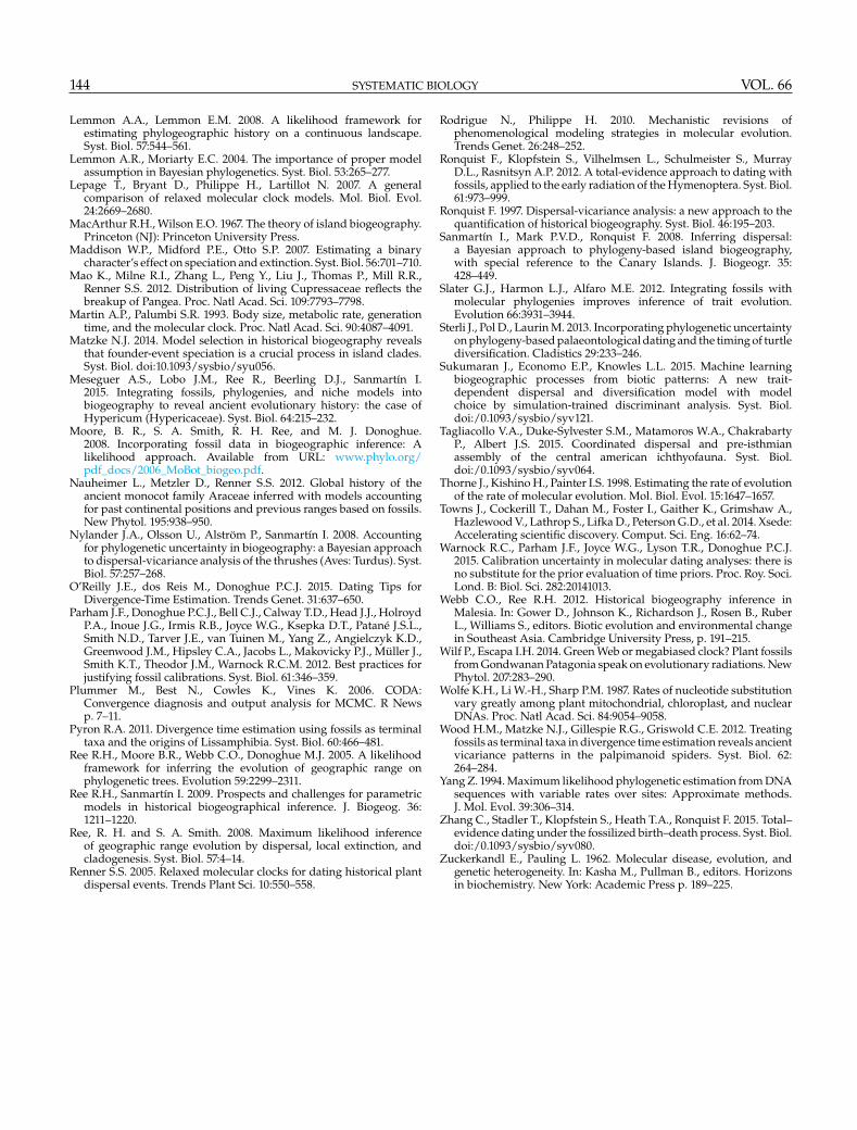
144 SYSTEMATIC BIOLOGY VOL. 66
Lemmon A.A., Lemmon E.M. 2008. A likelihood framework forestimating phylogeographic history on a continuous landscape.Syst. Biol. 57:544–561.
Lemmon A.R., Moriarty E.C. 2004. The importance of proper modelassumption in Bayesian phylogenetics. Syst. Biol. 53:265–277.
Lepage T., Bryant D., Philippe H., Lartillot N. 2007. A generalcomparison of relaxed molecular clock models. Mol. Biol. Evol.24:2669–2680.
MacArthur R.H., Wilson E.O. 1967. The theory of island biogeography.Princeton (NJ): Princeton University Press.
Maddison W.P., Midford P.E., Otto S.P. 2007. Estimating a binarycharacter’s effect on speciation and extinction. Syst. Biol. 56:701–710.
Mao K., Milne R.I., Zhang L., Peng Y., Liu J., Thomas P., Mill R.R.,Renner S.S. 2012. Distribution of living Cupressaceae reflects thebreakup of Pangea. Proc. Natl Acad. Sci. 109:7793–7798.
Martin A.P., Palumbi S.R. 1993. Body size, metabolic rate, generationtime, and the molecular clock. Proc. Natl Acad. Sci. 90:4087–4091.
Matzke N.J. 2014. Model selection in historical biogeography revealsthat founder-event speciation is a crucial process in island clades.Syst. Biol. doi:10.1093/sysbio/syu056.
Meseguer A.S., Lobo J.M., Ree R., Beerling D.J., Sanmartín I.2015. Integrating fossils, phylogenies, and niche models intobiogeography to reveal ancient evolutionary history: the case ofHypericum (Hypericaceae). Syst. Biol. 64:215–232.
Moore, B. R., S. A. Smith, R. H. Ree, and M. J. Donoghue.2008. Incorporating fossil data in biogeographic inference: Alikelihood approach. Available from URL: www.phylo.org/pdf_docs/2006_MoBot_biogeo.pdf.
Nauheimer L., Metzler D., Renner S.S. 2012. Global history of theancient monocot family Araceae inferred with models accountingfor past continental positions and previous ranges based on fossils.New Phytol. 195:938–950.
Nylander J.A., Olsson U., Alström P., Sanmartín I. 2008. Accountingfor phylogenetic uncertainty in biogeography: a Bayesian approachto dispersal-vicariance analysis of the thrushes (Aves: Turdus). Syst.Biol. 57:257–268.
O’Reilly J.E., dos Reis M., Donoghue P.C.J. 2015. Dating Tips forDivergence-Time Estimation. Trends Genet. 31:637–650.
Parham J.F., Donoghue P.C.J., Bell C.J., Calway T.D., Head J.J., HolroydP.A., Inoue J.G., Irmis R.B., Joyce W.G., Ksepka D.T., Patané J.S.L.,Smith N.D., Tarver J.E., van Tuinen M., Yang Z., Angielczyk K.D.,Greenwood J.M., Hipsley C.A., Jacobs L., Makovicky P.J., Müller J.,Smith K.T., Theodor J.M., Warnock R.C.M. 2012. Best practices forjustifying fossil calibrations. Syst. Biol. 61:346–359.
Plummer M., Best N., Cowles K., Vines K. 2006. CODA:Convergence diagnosis and output analysis for MCMC. R Newsp. 7–11.
Pyron R.A. 2011. Divergence time estimation using fossils as terminaltaxa and the origins of Lissamphibia. Syst. Biol. 60:466–481.
Ree R.H., Moore B.R., Webb C.O., Donoghue M.J. 2005. A likelihoodframework for inferring the evolution of geographic range onphylogenetic trees. Evolution 59:2299–2311.
Ree R.H., Sanmartín I. 2009. Prospects and challenges for parametricmodels in historical biogeographical inference. J. Biogeog. 36:1211–1220.
Ree, R. H. and S. A. Smith. 2008. Maximum likelihood inferenceof geographic range evolution by dispersal, local extinction, andcladogenesis. Syst. Biol. 57:4–14.
Renner S.S. 2005. Relaxed molecular clocks for dating historical plantdispersal events. Trends Plant Sci. 10:550–558.
Rodrigue N., Philippe H. 2010. Mechanistic revisions ofphenomenological modeling strategies in molecular evolution.Trends Genet. 26:248–252.
Ronquist F., Klopfstein S., Vilhelmsen L., Schulmeister S., MurrayD.L., Rasnitsyn A.P. 2012. A total-evidence approach to dating withfossils, applied to the early radiation of the Hymenoptera. Syst. Biol.61:973–999.
Ronquist F. 1997. Dispersal-vicariance analysis: a new approach to thequantification of historical biogeography. Syst. Biol. 46:195–203.
Sanmartín I., Mark P.V.D., Ronquist F. 2008. Inferring dispersal:a Bayesian approach to phylogeny-based island biogeography,with special reference to the Canary Islands. J. Biogeogr. 35:428–449.
Slater G.J., Harmon L.J., Alfaro M.E. 2012. Integrating fossils withmolecular phylogenies improves inference of trait evolution.Evolution 66:3931–3944.
Sterli J., Pol D., Laurin M. 2013. Incorporating phylogenetic uncertaintyon phylogeny-based palaeontological dating and the timing of turtlediversification. Cladistics 29:233–246.
Sukumaran J., Economo E.P., Knowles L.L. 2015. Machine learningbiogeographic processes from biotic patterns: A new trait-dependent dispersal and diversification model with modelchoice by simulation-trained discriminant analysis. Syst. Biol.doi:/0.1093/sysbio/syv121.
Tagliacollo V.A., Duke-Sylvester S.M., Matamoros W.A., ChakrabartyP., Albert J.S. 2015. Coordinated dispersal and pre-isthmianassembly of the central american ichthyofauna. Syst. Biol.doi:/0.1093/sysbio/syv064.
Thorne J., Kishino H., Painter I.S. 1998. Estimating the rate of evolutionof the rate of molecular evolution. Mol. Biol. Evol. 15:1647–1657.
Towns J., Cockerill T., Dahan M., Foster I., Gaither K., Grimshaw A.,Hazlewood V., Lathrop S., Lifka D., Peterson G.D., et al. 2014. Xsede:Accelerating scientific discovery. Comput. Sci. Eng. 16:62–74.
Warnock R.C., Parham J.F., Joyce W.G., Lyson T.R., Donoghue P.C.J.2015. Calibration uncertainty in molecular dating analyses: there isno substitute for the prior evaluation of time priors. Proc. Roy. Soci.Lond. B: Biol. Sci. 282:20141013.
Webb C.O., Ree R.H. 2012. Historical biogeography inference inMalesia. In: Gower D., Johnson K., Richardson J., Rosen B., RuberL., Williams S., editors. Biotic evolution and environmental changein Southeast Asia. Cambridge University Press, p. 191–215.
Wilf P., Escapa I.H. 2014. Green Web or megabiased clock? Plant fossilsfrom Gondwanan Patagonia speak on evolutionary radiations. NewPhytol. 207:283–290.
Wolfe K.H., Li W.-H., Sharp P.M. 1987. Rates of nucleotide substitutionvary greatly among plant mitochondrial, chloroplast, and nuclearDNAs. Proc. Natl Acad. Sci. 84:9054–9058.
Wood H.M., Matzke N.J., Gillespie R.G., Griswold C.E. 2012. Treatingfossils as terminal taxa in divergence time estimation reveals ancientvicariance patterns in the palpimanoid spiders. Syst. Biol. 62:264–284.
Yang Z. 1994. Maximum likelihood phylogenetic estimation from DNAsequences with variable rates over sites: Approximate methods.J. Mol. Evol. 39:306–314.
Zhang C., Stadler T., Klopfstein S., Heath T.A., Ronquist F. 2015. Total–evidence dating under the fossilized birth–death process. Syst. Biol.doi:/0.1093/sysbio/syv080.
Zuckerkandl E., Pauling L. 1962. Molecular disease, evolution, andgenetic heterogeneity. In: Kasha M., Pullman B., editors. Horizonsin biochemistry. New York: Academic Press p. 189–225.


![V. SPECIATION A. Allopatric Speciation B. Parapatric Speciation (aka Local or Progenitor - Derivative) C. Adaptive Radiation D. Sympatric Speciation [Polyploidy]](https://img.pdfslide.us/doc/110x75/56649d3f5503460f94a186e2/v-speciation-a-allopatric-speciation-b-parapatric-speciation-aka-local.jpg)