Embed Size (px)
Citation preview
1
BioEdit version 7.0.0
This is the current help file for BioEdit version 5.0.6.
Copyright ©1997-2004
Tom Hall
Ibis Therapeutics, a division of Isis Pharmaceuticals, Inc.
This is likely to be the final release of BioEdit.
There may be some bugs.
This is a free program and comes with a complete (but simple) disclaimer:
Simple DISCLAIMER: This software is provided as is. There are no warranties. The author
will not be held responsible for any problems. This software may be freely distributed, provided
that the original full installation is distributed along with the on-line documentation and the
license agreement, and that the distributer realizes that that are other freeware programs
packaged in the installation written by other authors.
That aside, if you have any questions or problems, you may email Tom Hall at:
This file was last updated on7/2/2004.
I would like to thank Isis Pharmaceuticals, Inc for generous support to the Brown lab (James
W. Brown, NCSU) for additions to BioEdit version 5.0.0, and for employment.
2
BioEdit Help Contents
Contents Page
About BioEdit .......................................................................................................................... 5 Introduction ................................................................................................................. .......... 5
BioEdit v7.0.0 features .......................................................................................... ............... 7
General overview of program and program organization ........................................................ 9
Known problems / Limitations ........................................................................................... .... 12
Contacting the Author ...................................................................................................... ..... 14
General use of BioEdit ........................................................................................................... 15 Sequence Editing / manipulation ............................................................................................ 15
Manual alignment of sequences ....................................................................................... 15
Tool Bar / Speed buttons ................................................................................................ 17
Editing in an Edit Box ............................................................................. ........................ 19
Windowshading .............................................................................................................. 21
Adding a new sequence ........................................................................ ........................... 21
Editing on screen .......................................................................................................... .. 21
Selecting Sequences ....................................................................................................... 21
Moving Sequences .......................................................................................................... 22
Cut/Copy/Paste ............................................................................................................... 22
Minimizing an Alignment ................................................................................................ 23
Basic manipulations / Sequence Menu ............................................................................. 23
Customizing the view ...................................................................................................... 29
Color table ...................................................................................................................... 31
Customizing menu shortcuts ........................................................................................... 32
Splitting the window view .............................................................................................. 33
Sorting sequences ........................................................................................................... 34
Graphical Feature Annotations ........................................................................................ 35
Adding, modifying and deleting sequence features manually ..................................... 36
Annotating sequences automatically from existing GenBank FEATURES data ......... 39
Annotating other sequences based upon an annotated template ................................. 41
Grouping sequences into groups or families ..................................................................... 42
Verbal confirmation of sequences .................................................................................... 43
Valid residue characters vs non-residue characters ........................................................... 44
Locking a sequence to prevent accidental edits ................................................................ 45
Anchoring a column ……………………………………………………………………….. 45
Comments ................................................................................................................... .... 46
Phylogenetic Tree Viewer ………………………………………………………………….46
Importing Phylogenetic Trees into an alignment ………………………………………….. 48
File formats ............................................................................................................... ............. 50
File formats that BioEdit currently reads and writes ......................................................... 50
BioEdit Project File Format ...................................................................................... 51
GenBank Format ...................................................................................................... 52
Fasta Format ............................................................................................................ 56
NBRF/PIR format .................................................................................................... 57
Phylip 3.2/2 format ................................................................................................... 58
Phylip 4 format ......................................................................................................... 59
ABI autosequencer files ............................................................................................ 60
Saving sequence annotation information .......................................................................... 63
Reading files in a Macintosh program .............................................................................. 63
3
Contents, continued Page
Toggling between nucleotide and protein views ...................................................................... 64
Printing .................................................................................................................. ................ 65
Exporting as raw text ...................................................................................................... ....... 66 Exporting as rich text ........................................................................ .................................... 66
Shaded graphic view of alignment .......................................................................................... 66
Information-based shading in the alignment window .............................................................. 70
Restriction Maps ........................................................................................................... ........ 72
Restriction Enzyme Browser ................................................................................................. 74
Codon tables ............................................................................................................... .......... 75
Six-frame translation .............................................................................................................. 77
Plasmid drawing ............................................................................................................ ......... 79
Searching functions ................................................................................................................ 84
Simple search: Find and Find Next .................................................................................. 84
Find in Titles and Find in Next Title ................................................................................ 84
Find Next ORF .............................................................................................................. . 84
Search for user-defined motif .......................................................................................... 85
Nucleic Acid ............................................................................................................ 85
Amino Acid ............................................................................................................. 86
Exact text match ...................................................................................................... 86
Exact including gaps ................................................................................................ 87
Preferences for translation output and ORF searching ............................................................ 88
Conservation plot view .......................................................................................................... 89
Basic Analysis Tools:
External Accessories ............................................................................................................... 90 Installing TreeView .............................................................................................................. .. 90
Configuring and Using External Applications ......................................................................... 91
Adding and configuring a new application ....................................................................... 92
Modifying an existing application configuration ............................................................... 97
Removing an accessory application ................................................................................. 98
Storage of the configuration information ......................................................................... 99
An example: Configuring ClustalW to run through a custom BioEdit interface ................ 101
BLAST ...................................................................................................................... ............ 106
BLAST Programs ........................................................................................................... 107
Local BLAST ................................................................................................................ . 107
Creating a database .................................................................................................. 107
Local BLAST searching ........................................................................................... 108
BLAST Internet Client .................................................................................................... 109
ClustalW ................................................................................................................... ............. 110
Using World Wide Web tools ................................................................................................. 112
Automated links ............................................................................................................ .. 112
Restriction mapping with Webcutter ........................................................................ 112
HTML BLAST with a Web Browser ........................................................................ 112
PSI-BLAST ............................................................................................................. 112
PHI-BLAST ............................................................................................................. 113
Prosite pattern and profile scans ............................................................................... 113
nnPredict protein secondary structure prediction ...................................................... 114
Other links ............................................................................................................................. 114
ENTREZ and PubMed .................................................................................................... 114
Pedro’s BioMolecular Research Tools ............................................................................ 114
Constructing World Wide Web bookmarks for BioEdit .......................................................... 115
4
Contents, continued Page
Analyses Incorporated into BioEdit ..................................................................................... 117
Amino Acid and Nucleotide Composition ............................................................................... 117
Entropy Plot .......................................................................................................................... 119
Hydrophobicity Profiles ................................................................................................... ...... 121
Identity Matrix ............................................................................................................ ........... 125
Nucleic Acid Translation with Codon Usage .......................................................................... 126
Positional nucleotide numerical summary ............................................................................... 129
Search for conserved regions of an alignment ........................................................... .............. 130
Dot Plot of two sequences .................................................................................................. ... 133
Pairwise sequence alignment ....................................................................... ........................... 134
Preferences for optimal pairwise alignment ...................................................................... 140
Substitution matrices used for pairwise alignment and alignment shading ................................ 141
Consensus sequences ........................................................................................................ ...... 147
RNA comparative analysis ..................................................................................................... 148
The basis of phylogenetic comparative analysis ............................................................... 148
Using Masks ........................................................................................... ........................ 150
Covariation ................................................................................................................ ...... 151
Covariation example ................................................................................................. 151
Using Covariation in BioEdit .................................................................................... 154
Table output ............................................................................ ......................... 155
List output ........................................................................................................ 156
Covariation analysis preferences .............................................................. ................. 157
The covariation algorithm ......................................................................................... 158
Potential Pairings ...................................................................................... ...................... 160
Potential pairings example ........................................................................................ 160
Using Potential Pairings in BioEdit .................................................................. ......... 163
List output ........................................................................................................ 164
Table output ................................................................................................ ...... 166
Potential pairings analysis preferences ....................................................................... 167
The potential pairings algorithm ................................................................................ 168
Mutual Information Analysis ............................................................................................ 169
General Overview of mutual Information .................................................................. 169
Mathematical Overview of Mutual Information ......................................................... 171
Using Mutual Information in BioEdit ....................................................................... 173
Mutual Information Example .................................................................................... 175
Sample RNA structure ....................................................................................... 176
Sample Alignment for Mutual Information ......................................................... 177
N-best sample output ........................................................................................ 179
Mutual Information Plot Example ...................................................................... 181
Setting Mutual Information Preferences .......................................................................... 182
Using the Matrix Plotter for Mutual Information Data ..................................................... 184
1-D plots of matrix data rows and columns ...................................................................... 188
The Mutual Information Examiner ................................................................................... 190
5
About BioEdit
Introduction
BioEdit version 7.0.0
Copyright ©1997-2004
Tom Hall
Current version built 7/2/2004
BioEdit is a biological sequence editor that runs in Windows 95/98/NT/2000/XP and is
intended to provide basic functions for protein and nucleic sequence editing, alignment,
manipulation and analysis. BioEdit is not a powerful sequence analysis program, but offers
many quick and easy functions for sequence editing, annotation and manipulation, as well as a
few links to external sequence analysis programs. Sequence lengths and numbers are limited
only by available system memory. Alignments >100 Mb have been edited on an average desktop
with reasonable efficiency. The document interface was originally modeled after the very nice
programs SeqApp and SeqPup by Don Gilbert. SeqApp (Macintosh) and SeqPup (cross-
platform) are offered free of charge from Indiana University at:
ftp://iubio.bio.indiana.edu/molbio/seqpup/
An exceptional alignment program that is freely available for Windows 95/98/2000 is called
GeneDoc. GeneDoc is very professional and has nice protein alignment annotation and analysis,
shading and structural definition features not offered in BioEdit, as well as an internal
phylogenetic tree view of alignments. GeneDoc can also be found on the World Wide Web:
http://www.psc.edu/biomed/genedoc/
BioEdit is a C++ program written in Borland's C++ Builder. I am a graduate student in
Microbiology at North Carolina State University, and not a trained programmer. This was my
introduction to the C++ language and is necessarily a side project (this is not part of my doctoral
work). This program could be much smaller and more efficient. Nevertheless, BioEdit provides
an easy means for sequence alignment, output, and some analyses.
6
BioEdit Features
The main goal of BioEdit is to provide a useful tool for biologists who do not want to have to
know much about a program to utilize it. BioEdit is intuitive, menu-driven, and highly graphical
and offers a graphical interface for users to run external analysis programs. The main functions
are intended to be visible by simply playing with the menu options.
Version 7.0.0 offers the following features:
An easy, graphical interface for sequence manipulation and editing.
Variable editing options, including ‘select and drag’ sliding and 'grab and drag' sliding of
residues, variable selection options, mouse-click insert and delete of gaps, full column
selecting, on-screen editing with cut, copy and paste, and auto-scrolling of edit window.
Split the window vertically or horizontally to manipulate two regions of an alignment at the
same time.
Collapse multiple columns of an alignment to hide them on the screen.
Anchor alignment columns to protect fixed regions in an alignment.
Automatically and manually annotate sequences with features such as introns, exons,
promoters, CDS, and all standard GenBank feature types. Automatically annotate other
sequences in an alignment using one sequence as a template.
Download sequences into an alignment document directly from GenBank.
Group sequences into color-coded families and lock group members for synchronized hand-
alignment.
User-defined character-relevance (any characters can be set to be considered as relevant
bases in nucleic acid or amino acid sequences for the purposes of similarity shading,
sequence identity matrices, and conservation plot views.
User-defined motif searching using standard Prosite nomenclature and utilizing IUPAC
characters to allow searching in nucleic acid or amino acid sequences, as well as exact text
searches including or ignoring gaps.
Lines may be defined as DNA, RNA, nucleic acid, protein, undefined, comments, sequence
mask (basically the same as comments) or RNA structure mask. Comments may be used to
hold general notes or things such as secondary structure mask definitions, but do not
contribute to conservation calculations.
Configure accessory application interfaces to run external analysis programs through a
graphical interface created by BioEdit. Automatically feed information to and retrieve files
from external apps. External apps run in a separate thread to allow simultaneous use of
BioEdit while running time-consuming processes. Output from an external program may be
automatically opened by another program.
Merge alignments through a common reference sequence.
7
Append one alignment to the end of another
Rudimentary phylogenetic tree viewer that supports node flipping and printing.
Display, print and edit ABI trace files from ABI autosequencer model 377, 373, and 3700, as
well as SCF files of version 2 and 3, such as the files output by Licor sequencers.
RNA comparative analysis tools, including covariation, potential pairings, and mutual
information analyses.
2-D matrix plotter for mutual information output with dynamic data viewing with the mouse
pointer. (Also allows image copy/paste and bitmap save).
Interactive 1-D plots of mutual information matrix rows and columns.
Color RNA secondary structure by base-pairs based upon a structure definition mask.
Save sequence annotation information in BioEdit or GenBank format
Align protein-encoding nucleic acid sequences through amino acid translation. Slide
residues in toggled hybrid protein-DNA translations by toggling translation of annotated
CDS features.
Search for conserved regions in an alignment (find good PCR targets or help define motifs)
Search for user-defined motifs in nucleic acid or protein sequences or search exact text with
wildcards and choice of including or ignoring gaps.
Dynamic memory allocation. Alignment size, number and length of sequences are limited
only by avalailable memory.
BioEdit currently reads and writes GenBank, Fasta, NBRF/PIR, Phylip 3.2 and Phylip 4
formats and reads ClustalW and GCG formats.
Import/Export filter for 10 additional formats (Using Don Gilbert’s ReadSeq).
Import/Append one file on to the end of another (regardless of file format).
Read and write large alignment files quickly with the BioEdit Project file format.
ClustalW multiple sequence alignment (interface internal, external program by Des Higgins
et. al.) with auto-update of aligned protein full titles and GenBank field information, as well
as nucleotide coding sequence when aligned from a protein view of nucleotide sequences.
Block copying of residues or sequence titles to clipboard allowing for pasting of full
alignments or parts of alignments into a word processor or spreadsheet.
Paste over blocks of sequence or sequence titles.
Basic sequence manipulations (copy/paste of sequences between documents, translation and
degenerate encoding, RNA->DNA->RNA, reverse/complement, upper/lowercase).
Multiple document interface (Maximum of 50 open alignment documents at a time, but no
set limit on other open windows).
Six-Frame translation of nucleic acid sequences into Fasta-format ORF lists. Tested by
translating the E. coli genome (4.6 Mbases) into 10,125 sorted raw codon stretches of 100 or
more amino acids and 39,880 unsorted raw codon stretches of 50 or more amino acids.
Semi-automated plasmid/vector drawing and annotation with vectored graphics, automatic
restriction site and positional marking, automated polylinker view, and user-controlled
drawing objects
Save plasmid files as editable vectored graphic files or as bitmaps, copy to other graphics
applications, and print plasmids at printer’s full resolution.
Amino acid and nucleotide composition summaries and plots
'Revert to Saved' and 'undo'/’redo’ functions (up to 30 undo levels allowed).
Edit both amino acid and nucleic acid sequences.
8
Easy point-and-click color table editing, with different tables for protein and nucleic acid
sequences.
Alignment-responsive shading based on information content of alignment positions.
Basic rich-text editor.
Internal restriction mapping utility with any or all-frames translation, multiple enzyme and
output options, including enzyme suppliers, and circular DNA option. Annotate sequences
with restriction sites, fragment sequences with exact monoisotopic mass calculation of all
resulting fragment strands.
Browse restriction enzymes by manufacturer, or choose enzymes by properties or from a list.
Auto-linking to your favorite Web Browser (e.g., Netscape or Internet Explorer).
World Wide Web Bookmarks.
NCBI BLAST tools, including BLAST 3.0 Internet client and local BLAST with the ability
to compile local databases from Fasta files
Configurable formatted text print with dynamic print preview,
Configurable formatted shaded graphical output with dynamic preview, identity and
similarity shading, and ability to cut and paste directly to graphics/presentation program for
generation of figures.
Entropy (lack of information) plotting of alignments
Hydrophobicity profiles of multiple proteins using several hydrophobicity scales, with
variable window width and option to analyze degapped sequences or alignments.
Retain data from GenBank files, including LOCUS, DEFINITION, ACCESSION,
VERSION, PID/SID, SOURCE, DBSOURCE, FEATURES, KEYWORDS, REFERENCE,
FEATURES and COMMENT.
Add table-based taxonomy data, as well as the NCBI-defined semicolon-delimited phylogeny
string. Automatically map Bacterial phylogenies to a columnized phylogeny table. Map
other phylogenies to your own curated phylogeny table.
A variety of search functions, including all GenBank fields and phylogeny table.
A variety of title search functions including a flexible search and replace using wilcards.
Several sort functions, including phylogeny-based sorting.
Calculate exact monoisotopic masses for DNA and RNA molecules.
Rudimentary FTICR mass-spec data viewer foir BRUKER FTICR acqus+fid data files.
Calculate oligo Tms with oligo/target mismatches based on mismatch parameters from John
SantaLucia’s lab.
Automatically grab Pubmed references associated with sequences directly from the web
(requires Internet Explorer as an ActiveX component).
Multiple levels of undo (up to 30), with more complete coverage of undoable operations (all
should theoretically be undoable, but there have been some oversights in previous versions).
9
General overview of program and program organization
BioEdit was originally written in Borland C++ Builder 3.0 (started in C++ Builder 1.0). At
the time, this was Borland’s newest C++ product which combined Borland C++ 5 with the
Visual Component Library (VCL) of Delphi, allowing for visual development of the user
interface. The benefit of using a Rapid Application Development (RAD) environment such as
this is that it allows for the easy creation of a very rich graphical interface. The drawback is that
the code is not portable. BioEdit runs only in Windows 95, 98, NT, 2000 and XP.
Organization: BioEdit currently supports the simultaneous editing of up to 50 documents. A
main control form contains menus to open documents, create new documents, set global options
such as color tables, codon table, and analysis preferences, and a window manager. Originally,
each document had its own complete set of menus for all manipulations confined to that
document, however, this has been abandoned for a more traditional multiple document interface.
BioEdit does not use excessive physical memory (unless big alignments are being edited), but it
does appear to be a bit of a resource hog. An alignment document currently has no set limit on
number of sequences or sequence length.
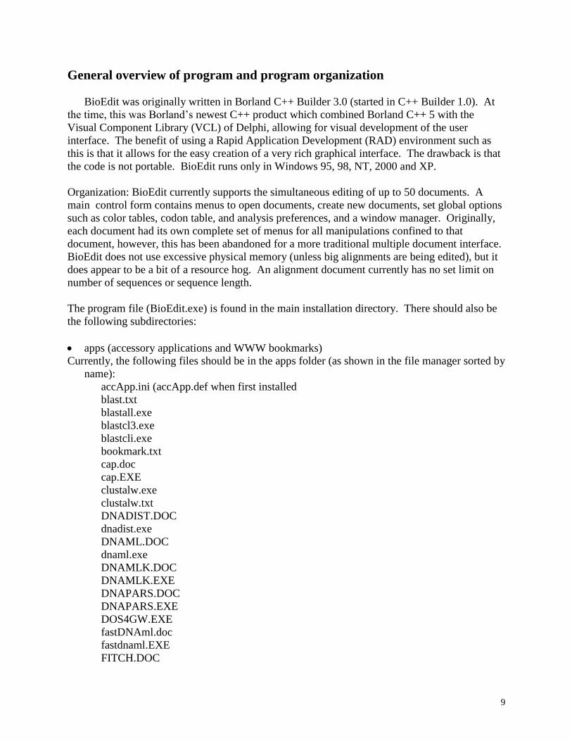
The program file (BioEdit.exe) is found in the main installation directory. There should also be
the following subdirectories:
apps (accessory applications and WWW bookmarks)
Currently, the following files should be in the apps folder (as shown in the file manager sorted by
name):
accApp.ini (accApp.def when first installed
blast.txt
blastall.exe
blastcl3.exe
blastcli.exe
bookmark.txt
cap.doc
cap.EXE
clustalw.exe
clustalw.txt
DNADIST.DOC
dnadist.exe
DNAML.DOC
dnaml.exe
DNAMLK.DOC
DNAMLK.EXE
DNAPARS.DOC
DNAPARS.EXE
DOS4GW.EXE
fastDNAml.doc
fastdnaml.EXE
FITCH.DOC
10
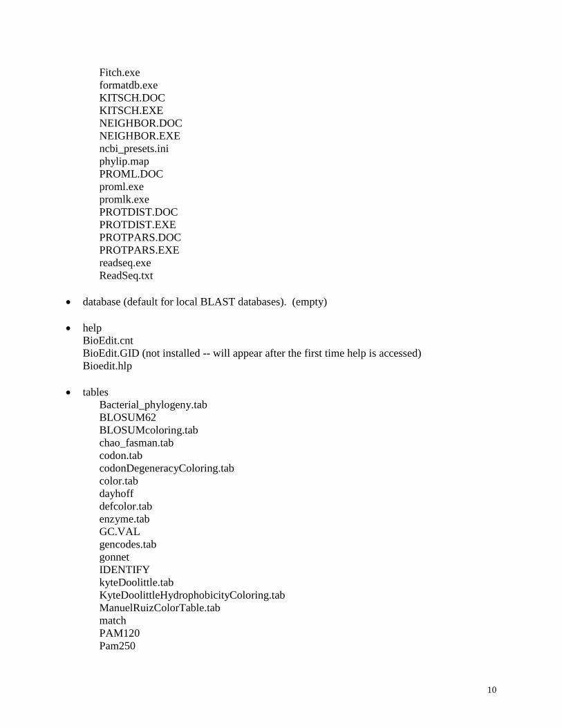
Fitch.exe
formatdb.exe
KITSCH.DOC
KITSCH.EXE
NEIGHBOR.DOC
NEIGHBOR.EXE
ncbi_presets.ini
phylip.map
PROML.DOC
proml.exe
promlk.exe
PROTDIST.DOC
PROTDIST.EXE
PROTPARS.DOC
PROTPARS.EXE
readseq.exe
ReadSeq.txt
database (default for local BLAST databases). (empty)
help
BioEdit.cnt
BioEdit.GID (not installed -- will appear after the first time help is accessed)
Bioedit.hlp
tables
Bacterial_phylogeny.tab
BLOSUM62
BLOSUMcoloring.tab
chao_fasman.tab
codon.tab
codonDegeneracyColoring.tab
color.tab
dayhoff
defcolor.tab
enzyme.tab
GC.VAL
gencodes.tab
gonnet
IDENTIFY
kyteDoolittle.tab
KyteDoolittleHydrophobicityColoring.tab
ManuelRuizColorTable.tab
match
PAM120
Pam250
11
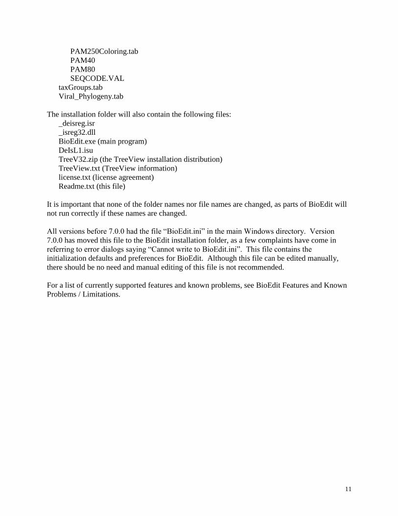
PAM250Coloring.tab
PAM40
PAM80
SEQCODE.VAL
taxGroups.tab
Viral_Phylogeny.tab
The installation folder will also contain the following files:
_deisreg.isr
_isreg32.dll
BioEdit.exe (main program)
DeIsL1.isu
TreeV32.zip (the TreeView installation distribution)
TreeView.txt (TreeView information)
license.txt (license agreement)
Readme.txt (this file)
It is important that none of the folder names nor file names are changed, as parts of BioEdit will
not run correctly if these names are changed.
All versions before 7.0.0 had the file “BioEdit.ini” in the main Windows directory. Version
7.0.0 has moved this file to the BioEdit installation folder, as a few complaints have come in
referring to error dialogs saying “Cannot write to BioEdit.ini”. This file contains the
initialization defaults and preferences for BioEdit. Although this file can be edited manually,
there should be no need and manual editing of this file is not recommended.
For a list of currently supported features and known problems, see BioEdit Features and Known
Problems / Limitations.
12
Known problems / Limitations
BioEdit is intended to be a general-purpose interface for several simple sequence manipulations,
general alignment of sequences with an option for automated multiple alignment, optimal
pairwise alignment, and an emphasis on making hand alignment easy. Several accessory
functions have been added over time (plasmid drawing, restriction mapping, ABI and SCF
viewing, RNA comparative analysis and graphical annotation among other features). However,
sophisticated search functions, specialized analyses such as protein secondary or tertiary
structure predictions, thermodynamic predictions of RNA structure, statistical analyses of
alignment quality, and probabilistic or neural network modeling of sequence patterns, alignment
and structure prediction are outside the scope of this program.
Although command-line accessory applications may be configured by the user, there are
programmed links to ClustalW and local BLAST and BLAST client 3. These links are not
guaranteed to work correctly if the Clustal program or BLAST programs are replaced with an
upgrade. Although the local BLAST and Clustal programs provided in the BioEdit installations
will continue to work, BLAST client 3 may not work correctly after the next time the NCBI
decides to change its client and I am no longer supporting this program directly. The source
code may be offered for download at a later date, but is somewhat disorganized, not well
commented, and really constrained to Borland C++ Builder (which is the main reason I don't
bother to post the source code).
Also, automated web links which feed a selected sequence to the web page (e.g. for BLAST,
PSI-BLAST, PROSITE profile scan) work by keeping a local HTML template for the web page,
the source for which BioEdit edits to include the selected sequence within the query text area.
Because of the highly mutable nature of the World Wide Web, these may not function correctly
for very long. If the server addresses change, or the HTML interface changes substantially, these
will no longer work correctly. They can possibly be updated by placing the newer web page
locally into the BioEdit/apps folder under the same name as the current ones, but whether they
work correctly will depend upon whether necessary URL references in the web page are
specified as absolute or relative paths, and whether they depend on calling local CGI or Java
programs, and other such potential problems.
The interface to configure command-line analysis programs does its best to be as complete as
possible without requiring a complicated general-purpose scripting language. Because of the
static nature of this interface and its options, however, there will be programs that just cannot be
run correctly through BioEdit, though most programs that accept a command line should be able
to be configured. Many people may prefer to run a program from the command line for better
control of the options, anyway. The accessory application configuration is mainly intended for
labs that want to be able to set up an easy method for several people who grew up on easy GUI
interfaces to be able to run routine analyses without having to navigate the files and command-
line options manually.
13
BioEdit performs fairly well with reasonably-sized alignments. However, there is an imposed
limit on both the number of alignment documents that can be opened at once, as well as the
number of sequences that can be contained in a single alignment. Currently the limit on open
alignment documents is 50, though this may run Windows out of resources. The limit on the
number of sequences in an alignment is 20,000.
The sequence number limit is independent of the lengths of the sequences. The absolute size of
an alignment matrix is limited only by available system memory. If a document runs the system
completely into virtual memory, editing will become very slow. If alignments on the scale of
several thousand rRNA genes, or sequence lists from entire genomes, for example, will be used,
it is recommended to have at least 64 to 128 Mb on a Win95/98 or NT machine, and probably at
least 128 Mb on a Win2000 machine.
The open document and sequence number limits are a result of poor original program design that
is a little cumbersome to change at this time. When the core of BioEdit first evolved, I was still
getting a handle on memory handling and pointer manipulations, and so a static array of pointers
to keep track of open documents by memory address or index is allocated at program startup, and
at the time of creation of a document, an array of pointers to hold sequences that can be accessed
either by memory address or array index is set aside. If this part of the core is ever redesigned,
there will be no restriction on sequence number nor document number.
Another potential drawback that becomes evident with very large documents is that all lists of
sequences are treated as an alignment matrix and the entire matrix is kept in physical memory for
every open document. Having three documents open that are each 8000 or so sequences of about
4000 bases long each, for example, will run memory just for the alignment matrices up to >96
Mb, which, on top of the OS and all other allocated memory, will run into virtual memory even
on a machine with 128 Mb RAM, and performance will slow to a crawl. At this time, there is no
monitoring of memory use, nor internal swap-file system to reduce physical memory usage of
idle matrix space.
The undo option is limited to one level at this point and needs to be redesigned (this probably
won't happen, though). One undo level requires the same amount of memory as the entire
alignment, and was admittedly programmed for ease of programming rather than performance.
Therefore, for an alignment matrix where N x M > 40,000,000 (N = number of sequences and M
= length of the longest sequence), undo is automatically disabled.
One more limitation is that BioEdit is written in Borland C++ Builder and is 100% Windows-
based. It is basically non-portable as it is. Since the majority of this program is its rich graphical
interface, creating a similar program on UNIX or Mac would require the program be written
almost from the ground up, with very little porting possible.
14
Contacting the Author The author can be reached at (at least until March, 2001):
Tom Hall
Department of Microbiology
North Carolina State University
4525 Gardner Hall
Box 7615, NCSU Campus
Raleigh, NC 27695
919-515-8803
15
General Use of BioEdit
Sequence Editing / Manipulation
Manual alignment of sequences
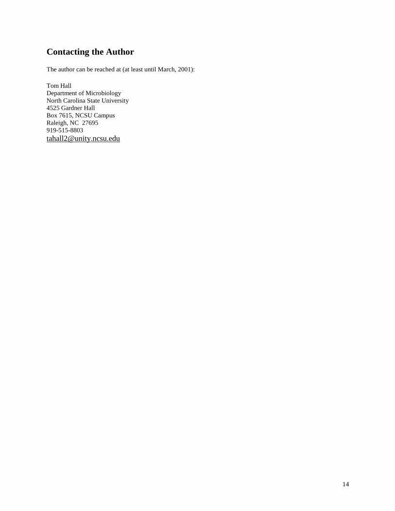
Below is an image of the basic BioEdit alignment document window.
Don’t worry if you don’t like the current view. The font, size, background color, residues colors,
and title window width may all be changed. The yellow box to the lower right of the mouse
arrow shows the absolute position in the current sequence. This also appears in the “Position”
caption on the control bar, and the option to shut off the yellow boxes is found under
View->show sequence position by mouse arrow.
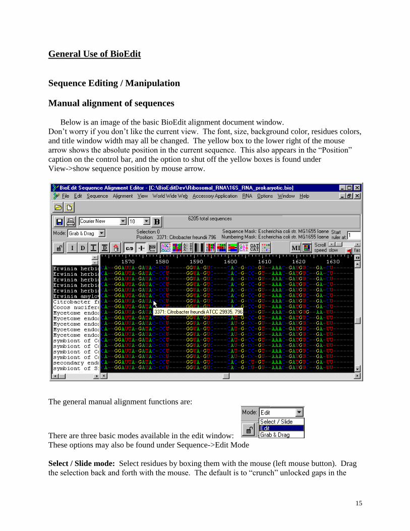
The general manual alignment functions are:
There are three basic modes available in the edit window:
These options may also be found under Sequence->Edit Mode
Select / Slide mode: Select residues by boxing them with the mouse (left mouse button). Drag
the selection back and forth with the mouse. The default is to “crunch” unlocked gaps in the
16
direction you are sliding and open new unlocked gaps on the other side of the selection. To
move the entire sequence downstream of the selection, regardless of gaps, hold down the shift
key while dragging. You may also toggle the appropriate button on the buttons panel (see
below) to change the default to moving the entire sequence downstream of the selection. With
this option selected, use the shift key to “crunch” unlocked gaps when sliding.
Using the shift key while selecting will select all residues between the current selection and
new selection. The CTRL key allows you to add only the new selection to the current selection
(for instance, you may want to select residues in three sequences which are not right next to each
other).
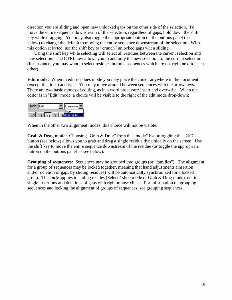
Edit mode: When in edit residues mode you may place the cursor anywhere in the document
(except the titles) and type. You may move around between sequences with the arrow keys.
There are two basic modes of editing, as in a word processor: insert and overwrite. When the
editor is in "Edit" mode, a choice will be visible to the right of the edit mode drop-down:
When in the other two alignment modes, this choice will not be visible.
Grab & Drag mode: Choosing “Grab & Drag” from the “mode” list or toggling the “G/D”
button (see below) allows you to grab and drag a single residue dynamically on the screen. Use
the shift key to move the entire sequence downstream of the residue (or toggle the appropriate
button on the buttons panel -- see below).
Grouping of sequences: Sequences may be grouped into groups (or "families"). The alignment
for a group of sequences may be locked together, meaning that hand adjustments (insertion
and/or deletion of gaps by sliding residues) will be automatically synchronized for a locked
group. This only applies to sliding resides (Select / slide mode or Grab & Drag mode), not to
single insertions and deletions of gaps with right mouse clicks. For information on grouping
sequences and locking the alignment of groups of sequences, see grouping sequences.
17
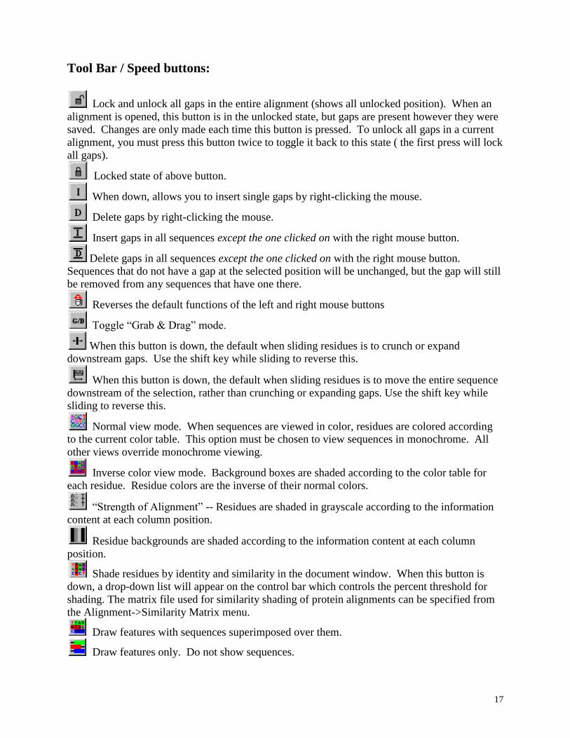
Tool Bar / Speed buttons:
Lock and unlock all gaps in the entire alignment (shows all unlocked position). When an
alignment is opened, this button is in the unlocked state, but gaps are present however they were
saved. Changes are only made each time this button is pressed. To unlock all gaps in a current
alignment, you must press this button twice to toggle it back to this state ( the first press will lock
all gaps).
Locked state of above button.
When down, allows you to insert single gaps by right-clicking the mouse.
Delete gaps by right-clicking the mouse.
Insert gaps in all sequences except the one clicked on with the right mouse button.
Delete gaps in all sequences except the one clicked on with the right mouse button.
Sequences that do not have a gap at the selected position will be unchanged, but the gap will still
be removed from any sequences that have one there.
Reverses the default functions of the left and right mouse buttons
Toggle “Grab & Drag” mode.
When this button is down, the default when sliding residues is to crunch or expand
downstream gaps. Use the shift key while sliding to reverse this.
When this button is down, the default when sliding residues is to move the entire sequence
downstream of the selection, rather than crunching or expanding gaps. Use the shift key while
sliding to reverse this.
Normal view mode. When sequences are viewed in color, residues are colored according
to the current color table. This option must be chosen to view sequences in monochrome. All
other views override monochrome viewing.
Inverse color view mode. Background boxes are shaded according to the color table for
each residue. Residue colors are the inverse of their normal colors.
“Strength of Alignment” -- Residues are shaded in grayscale according to the information
content at each column position.
Residue backgrounds are shaded according to the information content at each column
position.
Shade residues by identity and similarity in the document window. When this button is
down, a drop-down list will appear on the control bar which controls the percent threshold for
shading. The matrix file used for similarity shading of protein alignments can be specified from
the Alignment->Similarity Matrix menu.
Draw features with sequences superimposed over them.
Draw features only. Do not show sequences.
18
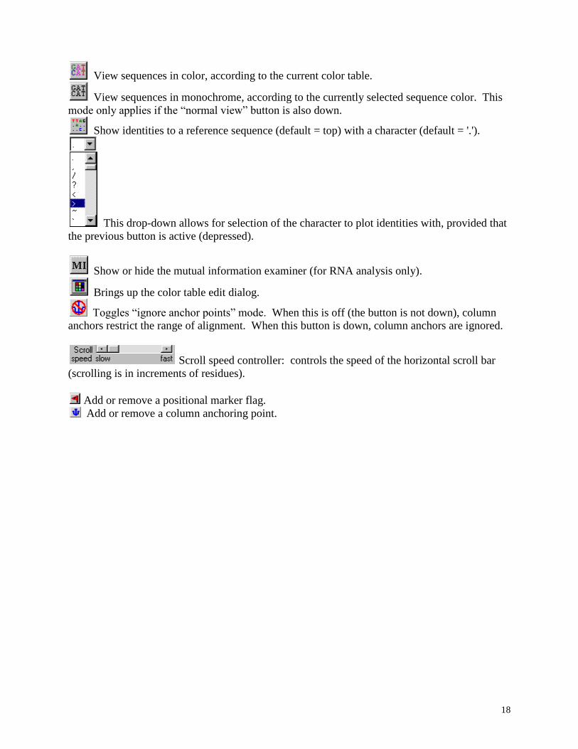
View sequences in color, according to the current color table.
View sequences in monochrome, according to the currently selected sequence color. This
mode only applies if the “normal view” button is also down.
Show identities to a reference sequence (default = top) with a character (default = '.').
This drop-down allows for selection of the character to plot identities with, provided that
the previous button is active (depressed).
Show or hide the mutual information examiner (for RNA analysis only).
Brings up the color table edit dialog.
Toggles “ignore anchor points” mode. When this is off (the button is not down), column
anchors restrict the range of alignment. When this button is down, column anchors are ignored.
Scroll speed controller: controls the speed of the horizontal scroll bar
(scrolling is in increments of residues).
Add or remove a positional marker flag.
Add or remove a column anchoring point.
19
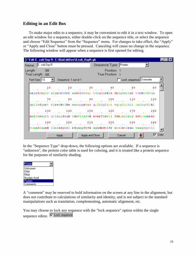
Editing in an Edit Box
To make major edits to a sequence, it may be convenient to edit it in a text window. To open
an edit window for a sequence, either double-click on the sequence title, or select the sequence
and choose “Edit Sequence” from the “Sequence” menu. For changes to take effect, the “Apply”
or “Apply and Close” button must be pressed. Canceling will cause no change in the sequence.
The following window will appear when a sequence is first opened for editing.
In the "Sequence Type" drop-down, the following options are available. If a sequence is
"unknown", the protein color table is used for coloring, and it is treated like a protein sequence
for the purposes of similarity shading.
A "comment" may be reserved to hold information on the screen at any line in the alignment, but
does not contribute to calculations of similarity and identity, and is not subject to the standard
manipulations such as translation, complementing, automatic alignment, etc.
You may choose to lock any sequence with the "lock sequence" option within the single
sequence editor.
20
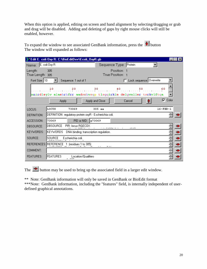
When this option is applied, editing on screen and hand alignment by selecting/dragging or grab
and drag will be disabled. Adding and deleting of gaps by right mouse clicks will still be
enabled, however.
To expand the window to see associated GenBank information, press the button
The window will expanded as follows:
The button may be used to bring up the associated field in a larger edit window.
** Note: GenBank information will only be saved in GenBank or BioEdit format
***Note: GenBank information, including the "features" field, is internally independent of user-
defined graphical annotations.
21
Windowshading
A document may be “Window shaded”, that is, reduced to its title bar, by double-clicking on
the title bar of the window. Double-clicking again will bring it back to its original size. It can
also be minimized and maximized in the normal manner.
Adding a new sequence
A new sequence may be added by:
1. Selecting the “New Sequence” option under the “Sequence” menu. The sequence may be
typed, or copied as raw text, into the sequence window. Press “Apply” to add the sequence to
the document.
2. Sequences may be copied and pasted from other BioEdit documents with the “Copy
Sequence(s)” and “Paste Sequence(s) commands from the “Edit” menu. Also, current menu
shortcuts may be used (defaults: Ctrl+F8 for copy and Ctrl+F9 for paste).
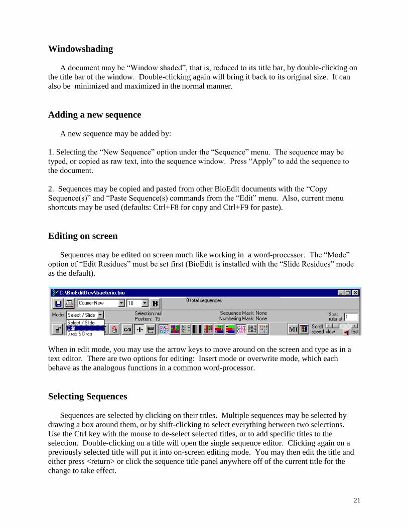
Editing on screen
Sequences may be edited on screen much like working in a word-processor. The “Mode”
option of “Edit Residues” must be set first (BioEdit is installed with the “Slide Residues” mode
as the default).
When in edit mode, you may use the arrow keys to move around on the screen and type as in a
text editor. There are two options for editing: Insert mode or overwrite mode, which each
behave as the analogous functions in a common word-processor.
Selecting Sequences
Sequences are selected by clicking on their titles. Multiple sequences may be selected by
drawing a box around them, or by shift-clicking to select everything between two selections.
Use the Ctrl key with the mouse to de-select selected titles, or to add specific titles to the
selection. Double-clicking on a title will open the single sequence editor. Clicking again on a
previously selected title will put it into on-screen editing mode. You may then edit the title and
either press <return> or click the sequence title panel anywhere off of the current title for the
change to take effect.
22
Moving Sequences
To move a sequence (or sequences), select it (highlight its title by clicking it with the left
mouse button) and drag it to where you would like it in the alignment.
Cut/Copy/Paste
Copy:
Text in edit window (sequence residues): Select the text with the mouse and choose “Copy” from
the “Edit” menu. Unlike a word processor, you may copy discreet blocks of text without
copying entire lines of text. A block of text copied this way may be pasted into any text edit-
capable program.
If, and only if, there are no residues selected in the entire document, sequences whose titles are
selected will be copied as BioEdit sequence structures to the BioEdit clipboard as well so that the
entire sequence(s) may be pasted into a document by choosing Paste Sequence(s).
Entire sequences: Select the sequence title(s) with the mouse and choose “Copy Sequence(s)”
from the “Edit” menu. Sequences whose titles are selected will also be copied to the Windows
Clipboard in Fasta format. More than one selected sequence will be copied to the clipboard as a
Fasta sequence list, and copied internally within BioEdit as a group of full BioEdit sequence
structures that can be pasted into any BioEdit document.
Note: The BioEdit "clipboard" which contains all sequence-related data (GenBank information,
graphical annotations) is internal to a single instance of BioEdit (they cannot be transferred
between independent processes). To copy sequences between BioEdit alignment documents,
make sure to have both documents open within the same instance of the program, as only Fasta-
formatted sequences are copied to the general Windows clipboard.
Paste:
Text in edit window: To paste into a sequence within the main edit window, the interface must
be in “Edit Residues” mode (see Editing On Screen). If a block of text is pasted into a sequence,
only the first line (defined by a carriage return) will be pasted in. This is to avoid possible
problems with pasting text into one sequence and inadvertently corrupting sequences below it.
To paste segments of text into a block of an alignment, segments must be pasted into sequences
one at a time. If the document is in “Slide Residues” or “Grab and Drag” mode, then Paste will
behave the same as Paste Sequence(s) (see below).
Entire sequences: From the menu of the document to paste sequences into, choose “Paste
Sequence(s)” from the “Edit” menu. The sequence(s) will be added to the end of the document.
They may be then be moved to somewhere else within the alignment.
23
“Cut” and “Cut Sequence(s)”: Same as “Copy” and “Copy Sequences”, but deletes copied
information from document. Residues are only deleted from the document if “Edit Residues”
mode is active, however. Also, when Cut is used when no residues are selected in the document,
sequences whose titles are selected are copied to the BioEdit Clipboard as sequence structures
and to the Windows Clipboard in Fasta format, but they are not deleted from the document. To
properly cut sequences from a document, choose “Cut Sequence(s)”.
Minimizing an Alignment
When an alignment is manipulated and tweaked extensively by hand, and when sequences
are periodically added to an existing alignment and aligned manually, gaps often result which are
present throughout a column in every sequence. To remove gaps that don’t change the actual
alignment, simply choose “Minimize Alignment” from the “Alignment” menu.
Basic Manipulations / Sequence Menu
There are a few simple sequence manipulations which can be done automatically with
BioEdit with a single menu option. These options are found in the “Sequence” menu.
Masking in BioEdit is at this point a little weak, and is provided mainly for use with the RNA
comparative analysis functions. For an explanation of how BioEdit uses masks, see Masks.
Lock and unlock gaps: A locked gap will not be compressed when residues within a sequence are
slid. To lock gaps, select the gaps to be locked and choose “Lock Gaps”. To lock all gaps in a
sequence, select the sequence title, then choose “Lock Gaps”. To lock all of the gaps for an
alignment, toggle lock/unlock button to the locked state:
Unlocking gaps is just the reverse of locking them. To unlock all gaps in an alignment, toggle
the locked/unlocked button to the unlocked state:
The “Degap” option will remove all selected unlocked gaps. It will also remove and all unlocked
gaps from sequences whose titles are selected.
Note: '~' and '.' (tilde and period) represent unlocked gaps, and '-' (dash) represents a locked gap.
These conventions are used throughout every window and function in BioEdit. A period is never
produced by BioEdit to represent a gap character, but is treated as a type of gap for computability
with programs that prefer this character. Also, some programs may use a period to represent
alignment positions that are neither residues nor gaps, but simply fill alignment slots before the
beginning or after the end of a sequence. BioEdit does not directly pay attention to this
distinction. Positions before or after a sequence's range are treated as gaps and BioEdit assumes
each alignment consists of truly homologous sequences (although BioEdit is also designed to
allow the user to ignore the alignment focus of the program and use it simply to manipulate lists
of sequences).
24
Sequence Menu (excluding the “mask” functions)
New Sequence: Create a new sequence. This opens up the single sequence editor
Edit Sequence: Opens the first selected sequence in the single sequence editor
Select Positions: Opens a dialog that allows selecting of specified positions in all selected
sequences.
Open at cursor position: If the document is in edit mode, and the cursor is showing, this
option will open the sequence with the cursor at the cursor’s current position in the single
sequence editor.
Rename: Rename sequence titles according to a submenu option:
Edit title: Change the title of a sequence on-screen.
with LOCUS: Change all selected titles to the LOCUS field.
with DEFINITION: Change all selected titles to the DEFINITION field.
with ACCESSION: Change all selected titles to the ACCESSION field.
with PID/NID: Change all selected titles to the PID or NID field.
Sort: Sort sequences according to the following criteria:
By Title
By Locus
By Definition
By Accession
By PID or NID
By Reference
By Comment
By residue frequency in a selected column
When the latter option (by residue frequency) is chosen, a single column of residues must
be selected, and the sort is performed by order of greatest frequency of residues defined
as valid residues.
Pairwise alignment: Optimal alignment of two sequences
Align two sequences (optimal GLOBAL alignment): Align two sequences optimally
with a global alignment algorithm based upon the Smith and Waterman optimal
alignment method.
Align two sequence (allow ends to slide): Align two sequences optimally with a local
alignment algorithm based upon the Gotoh modification of the Smith and Waterman
optimal alignment method which does not constrain the ends of either sequence (either
25
sequence end is allowed to slide freely over the other sequence). This alignment tends to
be very useful for quickly identifying overlapping regions of sequence reads in small
sequences where an auto-contig assembly program is not required.
Calculate identity/similarity for two sequences: Calculates the identity and similarity
(according to the current similarity matrix) for two sequences as they are currently
aligned in the document (does not align them).
Similarity Matrix (for pairwise alignments and shading): These matrices apply to amino acid
sequences only. BioEdit does not use any matrix scoring schemes for nucleic acids (only simple
identity).
BLOSUM62: The default matrix used by BLAST. The BLOSUM matrices are generally
good for database searches and assume moderately large evolutionary distances (smaller
BLOSUM number = greater evolutionary distance -- only the BLOSUM62 matrix
[intermediate] is supplied in BioEdit).
PAM40: Intended for very closely related sequences (40 PAM units = relatively small
evolutionary distance -- in the PAM matrices, large PAM number = greater evolutionary
distance).
PAM80
PAM120
PAM250: Intended for more distantly related sequences (larger PAM distance).
IDENTIFY: Simple match or mismatch matrix with a very large (-10000) penalty for
mismatches
DAYHOFF: Actually a PAM250 matrix -- M.O. Dayhoff's original PAM250 matrix
(each value rounded to the nearest integer).
MATCH: Simple match or mismatch matrix with a -1 penalty for mismatches and a +1
score for matches.
GONNET: A modified PAM250 matrix recommended by Gonnet (1992).
Features (Feature annotation functions):
Automatically annotate from GenBank Feature Fields: This option allows you to add
features according to the pre-existing GenBank data already deposited for the sequence.
Edit Features: Add, modify or delete features in a sequence.
Annotate Selection: Add a feature that will span the currently selected positions in all
sequences with a selection in them.
26
Annotate selected sequences using the first sequence as a template
Sequence groups (or families): Group and ungroup sequences and edit current groups.
Edit Mode: Sets the current editing mode. See Manual alignment of sequences.
Mask (covered above).
Toggle color: toggles coloring of single sequences. This is a left-over of an early version and is
pretty useless.
Gaps:
Lock gaps, Unlock gaps and Degap: explained above.
Insert multiple gaps: insert a variable number of gaps at the currently selected position in
the alignment window.
Manipulations: Simple manipulations that are independent of sequence type.
lowercase and UPPERCASE: As indicated -- sequences only, not titles.
Reverse: Reverses any sequence
Remove numbers: As indicated. This was added by request to ease the process of
pasting partial sequences from GenBank formatted text files and web pages.
World Wide Web:
Automated links are provided to the following selected WWW search functions:
BLAST, PSI-BLAST and PHI-BLAST.
Prosite profile and pattern scans
nnPredict protein secondary structure prediction
Nucleic Acid:
Nucleotide Composition: Plots nucleotide composition and gives a summary including
G+C and A+T percentages and molecular weight
Complement: The complement of a DNA or an RNA sequence. This option has no
effect upon protein sequences, and characters other than the standard five bases (A, G, C,
T and U) and purines/pyrimidines are not affected (the complement of a purine (“R”) is
a pyrimidine (“Y”)).
Reverse complement: Behaves the same as complement, but also reverses the sequence.
DNA->RNA and RNA->DNA: These really do nothing but toggle “T”’s and “U”’s and
change the sequence type.
27
Translate: Translate sequence in frame 1, 2 or 3, or translate the currently selected region
of a sequence. Codons are separated by spaces. The nucleotide sequence is shown on
top of the protein sequence. The translated sequence is specified by three-letter or one-
letter amino acid codes, depending on the preferences. If a selected part of a sequence is
translated sequence is translated, either the entire nucleic acid sequence or only the
translated region may be displayed, depending on the current preferences. A summary
table may be displayed below the translation which shows the number of times each
codon appears in the sequence, as well as the frequency with which each codon codes for
a particular amino acid according to the codon table provided.
Find Next ORF: Searches the currently selected sequences from the point of the last
current selection for ORFs according to the parameters defined in the preferences.
Create plasmid from sequence: A DNA sequence may be converted directly into a
plasmid/vector. A restriction map is automatically run on the sequence. For help on
annotating a plasmid, see Plasmid drawing with BioEdit
Restriction Map: Run a restriction map on a DNA or RNA sequence.
Sorted and Unsorted six frame translations: Translate nucleic acid sequences in all six
frames by specifying a start codon (ATG, “any”, or user-defined), and a minimum and
maximum ORF size. Sorted translations are limited to a few thousand output ORFs. To
get a raw translation of entire genome (or larger), use an unsorted translation (in an
unsorted translation, the output data is printed directly to a file, and very little memory is
required).
Protein:
Amino Acid composition: Gives a plot and summary of the amino acid composition of a
protein, including the molecular weight.
Hydrophobicity profiles:
Mean hydrophobicity is calculated by the method of Kyte and Doolittle (1982) using
a choice of hydrophobicity scales.
Hydrophobic moment is calculated according to the method of Eisenberg et. al.,
1984). The algorithm of Eisenberg et. al. for finding transmembrane alpha helices is
not applied here, rather the hydrophobic moment of a user defined segment of
sequence is plotted for each residue (each residue represents the beginning of a user-
defined segment);
Mean hydrophobic moment: For each residue, the mean hydrophobic moment for a
window the same size as that used to calculate each hydrophobic moment is applied.
28
Note: I do not have the expertise to make any claims about the predictive power of
these profile plots. BioEdit makes no conclusions about hydrophobic and/or
transmembrane segments of proteins, and interpretation of these plots is up to the
judgment of the user.
For a description of the method and meaning of these plots, and references to the
hydrophobicity scales and to hydrophobicity analysis algorithms, see Hydrophobicity
Profiles.
Translate or Reverse-Translate: Translation from DNA or RNA to protein is done according to
the codon table specified in the BioEdit.ini file. The default is “codon.tab” found in the /tables
directory. The default is the E. coli codon usage table produced by J. Michael Cherry
([email protected]) with the GCG program CodonFrequency. Any codon table
with this format may be used, but the codon table must be in this format to be recognized by
BioEdit. To choose a different table, see Codon Tables. A protein sequence will be
degenerately encoded (to DNA) based upon codon preference for each particular amino acid.
Obviously, if a nucleic acid sequence is translated to protein and back, information will be lost.
Translate in Selected Frame (Permanent): This allows you to translate a nucleotide sequence
as if the currently selected column (defined as the start of a selection if more than one column is
selected) is frame +1. When applied to a protein sequence, it simply results in the same
degenerate reverse translation as the above option.
Toggle Translation: Toggles nucleotide sequences between the nucleic acid and encoded
protein sequences, allowing for alignment of the sequences in either view. See Toggling
between nucleotide and protein views
Toggle Translation in selected frame: This option allows you to toggle the translated view
(without losing any nucleotide information) as if the currently selected column (defined as the
start of the selection if more than one column is selected) was in frame +1.
Dot Plot (pairwise comparison): Create a dot plot of two sequences compared to each other in
a matrix.
Customizing the View
BioEdit currently supports the following view options:
Background colors for sequence and title windows
Default monochrome sequence and title colors
Character fonts.
Font size
View sequences in bold-face type.
View sequences in monochrome or color (editing is faster in monochrome).
Normal color view (residues colored)
29
Inverse (background colored)
Strength of alignment: shading is based upon the information contained at each position --
information is calculated as follows:
DNA/RNA: information = ln5+fbx[ln(fbx)])
Protein: information = ln21+fbx[ln(fbx)]),
where fbx represents the frequency of each residue b occuring at position x. 5 represents the
number of possible residues for nucleic acid (4 nucleotides plus gaps). This is not quite right,
and the usefulness decreases if a lot of alternative characters are used. 21 represents the
number of possibilities for amino acids (including the gap). ln5 and ln21 are the maximum
information for a nucleic acid position or a protein position, respectively and the term
-fbx[ln(fbx)]) represents the entropy (a measure of variability) at the position.
The above description was true of BioEdit versions before 5.0.0. In BioEdit version 5.0.0,
only the user-defined valid residues contribute to the entropy calculation. In this case, gaps
only contribute to the calculation of entropy if they are defined as valid residues (or place-
holding characters, if you'd rather think of it that way, as it is obvious that a gap cannot be a
residue).
Strength of Alignment - Inverse: Same as Strength of alignment, but the background instead
of the residue is shaded.
Identity/Similarity shading: Residues are background-shaded with there color-table defined
colors if their frequency in a column equals or exceeds a user-defined cutoff (the option to
choose the cutoff goes in increments of 10% and is visible when this mode is active).
Nucleotide alignments are shaded according to identity only, while protein alignments are
shaded according to identity and similarity according to the currently selected amino acid
similarity scoring matrix. Only characters defined as valid residues and only non-comment
sequences contribute to the similarity and identity calculations.
Sequences and Graphical Features: Draw graphical sequence annotations on the document
screen with the sequences superimposed on top of them.
Graphical Features: Draw graphical sequence annotations in cartoon mode and do not draw
the residue characters. When this mode is active, there is a scale-factor slide bar toward the
top of the window that enables a scaling factor between 1:1 and 1:32768, by orders of 2.
Conservation plot: Residues are plotted as a user-defined character (default = a period) if
they are identical to the residue in the same column as a user-defined standard (default = the
top sequence). To change the standard (reference) sequence, right-click the sequence title
with the mouse that you want to be the new standard for the conservation plot. Only
characters set as valid residues are recognized for the identity plot.
Show or hide the mutual information examiner (this is only useful for RNA comparative
analysis).
Show or Hide the translation toggling control. This is mutually exclusive with the mutual
information examiner control, because of space limitations.
Show sequence position by mouse arrow: when moving the mouse over sequences in a
document window, the absolute position of the mouse (ignoring gaps) is reported on the
control bar above the sequence view window. The position may also e reported (including
the full length of the title) at the mouse arrow. This option turns this feature on or off.
Split window vertically: A duplicate window is created which sits inside the document
window and is synchronized with the current document. The window is placed such that the
document appears to be split by a vertical window splitter (it’s really just two synchronized
documents, one with most of it’s interface removed). The vertical scroll position of the two
30
windows stays in register, but horizontal scrolling in each is independent of the other. The
window may be resized by grabbing the window splitter within the main document. The
window may be returned to normal by choosing this menu option again.
Split window horizontally: A synchronized window is created which is placed directly
below the original window such that the border between the bottom of the original window
and the top of the new window behaves like a window splitter. Remove this window by
choosing the option again.
Save options as default: When “Auto-update view options” is off, choosing this item will
save the view options of the current document as the default for all newly created or newly
opened documents.
Auto-update view options: when this item is checked, all changes made to the document
views and preferences are automatically saved as the default for new documents.
Customize menu shortcuts: brings up a dialog that allows changing of menu shortcuts to any
key combination.
Hide control bar or Show control bar: The main control bar may be removed in order to fit
more sequences on the screen in a simple frame window. If the control bar is hidden, then
the “Show control bar” option is offered. If the control bar is hidden, sequence editing
modes may be changed through the Sequence->Edit Mode submenus. View defaults may be
changed via menus as well.
To change these settings, choose the appropriate option from the “View” menu of an open
document. To make the current view from any particular document into the default view for all
subsequently opened documents, choose “Save Options as Default”.
These views may be selected either through the “View” menu or by pressing the appropriate
speed button on in alignment window.
31
Color Table
One color table is used for all documents. This table is called “color.tab” and is found in the
\tables directory of the BioEdit install directory (see Program Organization). Although the table
may be edited by hand, it is much easier to use the “Color Table” option under the “Options”
menu of the main application control form.
Editing the color table: To edit the color table, choose “Color Table” from the “options” menu of
the main application control bar. There is a different color table for nucleotide and protein
sequences. To change the color of a residue, double-click on the colored box above the residue
to get a color dialog. To add or delete a residue, click the “+” or “-” button. In the window that
appears, push the button for the residue to be added or deleted. When adding a residue, it comes
in with black as the default color. The color must then be changed to the desired color.
To edit the color table by hand, the following format must be observed:
Each color table is denoted by a line containing the exact text “/amino acids/” or
“/nucleotides/” (without the double quotes).
The end of each table is denoted by (exactly) “/////” (without the double quotes);
Each residue color is specified by two lines in the file:
Line 1: A 3-byte hexadecimal number (or its integer value). The three bytes represent
the values for blue, green and red, respectively (backwards RGB).
Line 2: An unbroken list of all characters representing all characters which should have
this color. If a character color is redefined elsewhere in the file, the last occurrence will
be the valid one.
Note: Manual editing of the color table should not be necessary and is not recommended.
If the color table becomes corrupted, it may lead to program failure on startup or when the color
table is edited. If this happens, you may delete the color table and create a new one, one residue
at a time (you will get an error on startup and on choosing “Color Table”, but the program will
create a new table when the “Save Table” button is pressed). This is tedious, so the /tables folder
of BioEdit also comes with a file called “defcolor.tab”. If the color table becomes corrupted, you
can make a copy of defcolor.tab and change the name of the copy to “color.tab”.
32
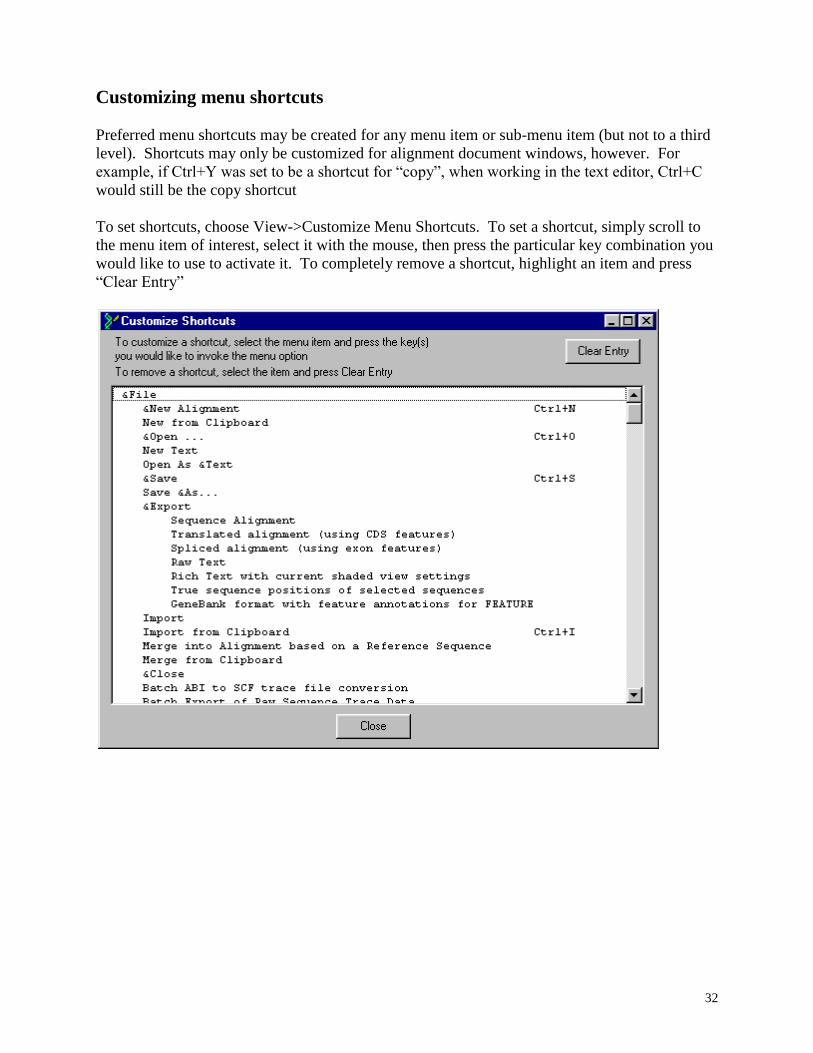
Customizing menu shortcuts
Preferred menu shortcuts may be created for any menu item or sub-menu item (but not to a third
level). Shortcuts may only be customized for alignment document windows, however. For
example, if Ctrl+Y was set to be a shortcut for “copy”, when working in the text editor, Ctrl+C
would still be the copy shortcut
To set shortcuts, choose View->Customize Menu Shortcuts. To set a shortcut, simply scroll to
the menu item of interest, select it with the mouse, then press the particular key combination you
would like to use to activate it. To completely remove a shortcut, highlight an item and press
“Clear Entry”
33
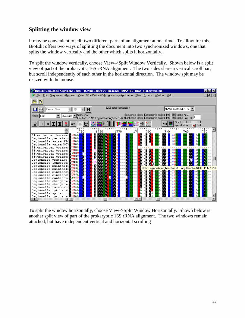
Splitting the window view
It may be convenient to edit two different parts of an alignment at one time. To allow for this,
BioEdit offers two ways of splitting the document into two synchronized windows, one that
splits the window vertically and the other which splits it horizontally.
To split the window vertically, choose View->Split Window Vertically. Shown below is a split
view of part of the prokaryotic 16S rRNA alignment. The two sides share a vertical scroll bar,
but scroll independently of each other in the horizontal direction. The window spit may be
resized with the mouse.
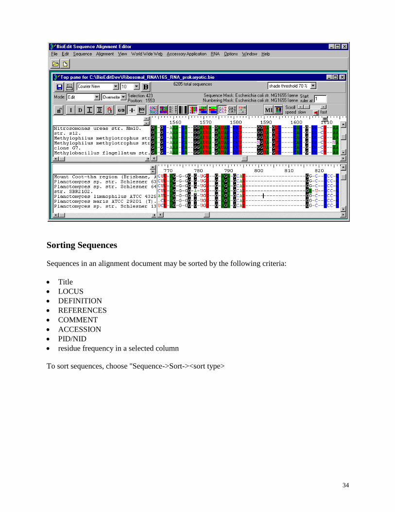
To split the window horizontally, choose View->Split Window Horizontally. Shown below is
another split view of part of the prokaryotic 16S rRNA alignment. The two windows remain
attached, but have independent vertical and horizontal scrolling
34
Sorting Sequences
Sequences in an alignment document may be sorted by the following criteria:
Title
LOCUS
DEFINITION
REFERENCES
COMMENT
ACCESSION
PID/NID
residue frequency in a selected column
To sort sequences, choose "Sequence->Sort-><sort type>
35
Graphical Feature Annotations
It is sometimes convenient to have information about certain elements of a sequence
(e.g., exons, introns, helices, motifs, etc.) available for reference in a quick and easy way,
without going to external sources such as a notebook, other files, or sources in the literature or on
the WWW. For this reason, functions allowing for the graphical annotation of sequence features
were added in version 5.0.0. Annotations may be done by hand, or automatically from existing
GenBank format FEATURES data. Names and descriptions for features that span any position
in a sequence are available right in the alignment window as ToolTips when the mouse arrow is
moved over the sequence residues. The standard GenBank format feature types are used as a
basis for internally keeping track of the sequence "type". If one is willing to adhere to GenBank
standards when defining the "description" of each feature, the feature annotation functions of
BioEdit can also provide a convenient way to annotate a sequence, or set of sequences, which
can be exported in standard GenBank format using the user-defined graphical features to fill in
the GenBank FEATURES field. This can be a useful starting point for a sequence submission
using Sequin or BankIt.
When a feature is added to a sequence in BioEdit manually, the "true" positions are
calculated and assumed to take precedent over the absolute positions in the alignment, and all
future alignment adjustments are handled with these "true" positions in mind. For example, if 5
gaps are deleted within a feature, the end of a feature is drawn back by five in the alignment, but
the absolute number of residues within the feature does not change. If 3 bases are deleted within
the feature, the actual end position of the feature will be moved back by three. Likewise, when
features are added automatically from GenBank information, the positions in the alignment
which correspond to the true start and end of each feature are calculated and updated to reflect
the correct aligned state of all elements. BioEdit allows control over the title of the feature, the
color, the shape (rectangular, oval, diamond or arrow), the direction (only makes a difference for
an arrow), the "type" (either "undefined" or any of the 67 standard GenBank feature types), and
reserves space for a description (unlimited in length).
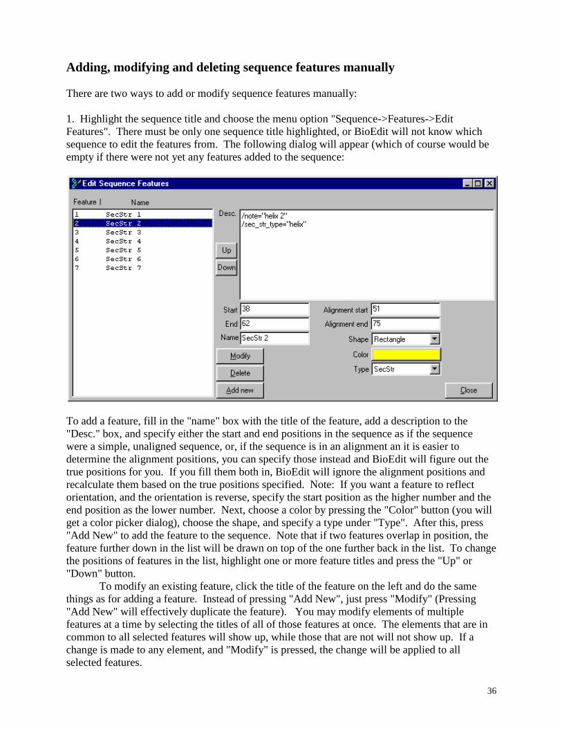
36
Adding, modifying and deleting sequence features manually
There are two ways to add or modify sequence features manually:
1. Highlight the sequence title and choose the menu option "Sequence->Features->Edit
Features". There must be only one sequence title highlighted, or BioEdit will not know which
sequence to edit the features from. The following dialog will appear (which of course would be
empty if there were not yet any features added to the sequence:
To add a feature, fill in the "name" box with the title of the feature, add a description to the
"Desc." box, and specify either the start and end positions in the sequence as if the sequence
were a simple, unaligned sequence, or, if the sequence is in an alignment an it is easier to
determine the alignment positions, you can specify those instead and BioEdit will figure out the
true positions for you. If you fill them both in, BioEdit will ignore the alignment positions and
recalculate them based on the true positions specified. Note: If you want a feature to reflect
orientation, and the orientation is reverse, specify the start position as the higher number and the
end position as the lower number. Next, choose a color by pressing the "Color" button (you will
get a color picker dialog), choose the shape, and specify a type under "Type". After this, press
"Add New" to add the feature to the sequence. Note that if two features overlap in position, the
feature further down in the list will be drawn on top of the one further back in the list. To change
the positions of features in the list, highlight one or more feature titles and press the "Up" or
"Down" button.
To modify an existing feature, click the title of the feature on the left and do the same
things as for adding a feature. Instead of pressing "Add New", just press "Modify" (Pressing
"Add New" will effectively duplicate the feature). You may modify elements of multiple
features at a time by selecting the titles of all of those features at once. The elements that are in
common to all selected features will show up, while those that are not will not show up. If a
change is made to any element, and "Modify" is pressed, the change will be applied to all
selected features.
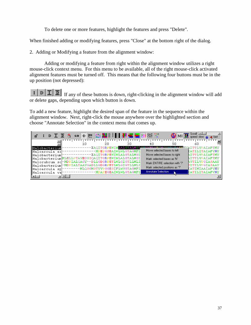
37
To delete one or more features, highlight the features and press "Delete".
When finished adding or modifying features, press "Close" at the bottom right of the dialog.
2. Adding or Modifying a feature from the alignment window:
Adding or modifying a feature from right within the alignment window utilizes a right
mouse-click context menu. For this menu to be available, all of the right mouse-click activated
alignment features must be turned off. This means that the following four buttons must be in the
up position (not depressed):
If any of these buttons is down, right-clicking in the alignment window will add
or delete gaps, depending upon which button is down.
To add a new feature, highlight the desired span of the feature in the sequence within the
alignment window. Next, right-click the mouse anywhere over the highlighted section and
choose "Annotate Selection" in the context menu that comes up.
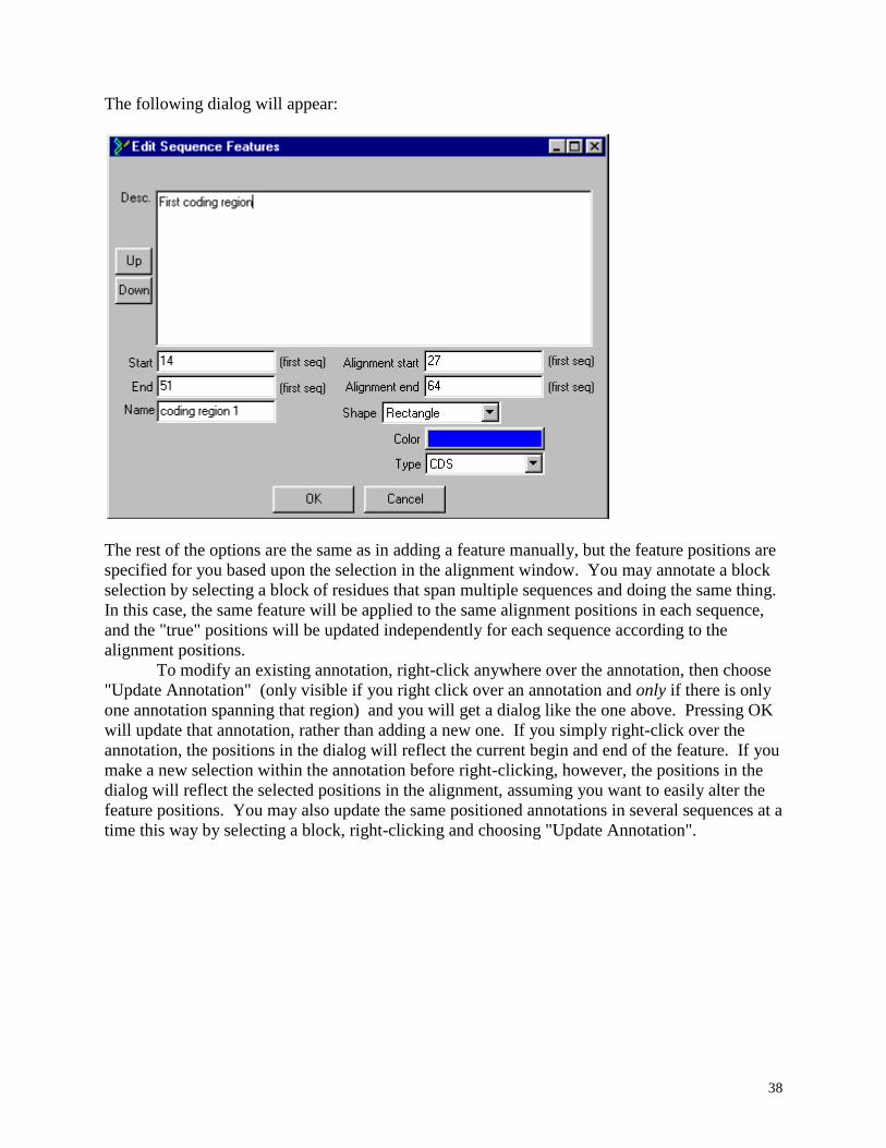
38
The following dialog will appear:
The rest of the options are the same as in adding a feature manually, but the feature positions are
specified for you based upon the selection in the alignment window. You may annotate a block
selection by selecting a block of residues that span multiple sequences and doing the same thing.
In this case, the same feature will be applied to the same alignment positions in each sequence,
and the "true" positions will be updated independently for each sequence according to the
alignment positions.
To modify an existing annotation, right-click anywhere over the annotation, then choose
"Update Annotation" (only visible if you right click over an annotation and only if there is only
one annotation spanning that region) and you will get a dialog like the one above. Pressing OK
will update that annotation, rather than adding a new one. If you simply right-click over the
annotation, the positions in the dialog will reflect the current begin and end of the feature. If you
make a new selection within the annotation before right-clicking, however, the positions in the
dialog will reflect the selected positions in the alignment, assuming you want to easily alter the
feature positions. You may also update the same positioned annotations in several sequences at a
time this way by selecting a block, right-clicking and choosing "Update Annotation".
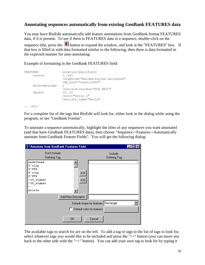
39
Annotating sequences automatically from existing GenBank FEATURES data
You may have BioEdit automatically add feature annotations from GenBank format FEATURES
data, if it is present. To see if there is FEATURES data in a sequence, double-click on the
sequence title, press the button to expand the window, and look at the "FEATURES" box. If
that box is filled in with data formatted similar to the following, then there is data formatted in
the expected manner for auto-annotating:
Example of formatting in the GenBank FEATURES field:
FEATURES Location/Qualifiers
source 1..247
/organism="Halobacterium salinarum"
/db_xref="taxon:2242"
NonStdResidue 1
/non-std-residue="PCA NH3+"
SecStr 10..31
/note="helix 1"
/sec_str_type="helix"
... etc.
For a complete list of the tags that BioEdit will look for, either look in the dialog while using the
program, or see "GenBank Format".
To annotate a sequence automatically, highlight the titles of any sequences you want annotated
(and that have GenBank FEATURES data), then choose "Sequence->Features->Automatically
annotate from GenBank Feature Fields". You will get the following dialog:
The available tags to search for are on the left. To add a tag or tags to the list of tags to look for,
select whatever tags you would like to be included and press the ">>" button (you can move any
back to the other side with the "<<" button). You can add your own tag to look for by typing it
40
into the "Add New Descriptor" box and pressing "Add New Descriptor", but all of the standard
GenBank tags should be available in the box on the left.
You may choose a default color to apply to all of the features, or you can let BioEdit
automatically choose colors for you (they can be edited later). If BioEdit chooses the colors, all
features of the same type will get the same color. If you choose a default color all features will
be the same color, regardless of type. You may also choose a default shape. The default for all
features is rectangular. The available shape options are: rectangle, oval, diamond and arrow. If
arrow is chosen, then the start and end positions are important for determining orientation of a
feature.
When BioEdit adds features, it searches through the FEATURES data looking for the
specific tags specified in the above dialog. When it finds one (formatted in the proper place), a
new feature is created. The title will be the feature type plus a number reflecting the present
number of that feature in the list (e.g. "exon 1", "intron 1", "exon 2", etc.). The description will
be all of the descriptive data that follows the tag in the file, including carriage returns to keep the
formatting correct. For example, a CDS feature might have the following name and description:
Name: CDS 2
Description:
/label=b0014
/gene="dnaK"
/product="DnaK protein (heat shock protein 70)"
/note="o638; 100 pct identical to DNAK_ECOLI SW: P04475"
/codon_start=1
/transl_table=11
/translation="MGKIIGIDLGTTNSCVAIMDGTTPRVLENAEGDRTTPSIIAYTQ
DGETLVGQPAKRQAVTNPQNTLFAIKRLIGRRFQDEEVQRDVSIMPFKIIAADNGDAW
VEVKGQKMAPPQISAEVLKKMKKTAEDYLGEPVTEAVITVPAYFNDAQRQATKDAGRI
AGLEVKRIINEPTAAALAYGLDKGTGNRTIAVYDLGGGTFDISIIEIDEVDGEKTFEV
LATNGDTHLGGEDFDSRLINYLVEEFKKDQGIDLRNDPLAMQRLKEAAEKAKIELSSA
QQTDVNLPYITADATGPKHMNIKVTRAKLESLVEDLVNRSIEPLKVALQDAGLSVSDI
DDVILVGGQTRMPMVQKKVAEFFGKEPRKDVNPDEAVAIGAAVQGGVLTGDVKDVLLL
DVTPLSLGIETMGGVMTTLIAKNTTIPTKHSQVFSTAEDNQSAVTIHVLQGERKRAAD
NKSLGQFNLDGINPAPRGMPQIEVTFDIDADGILHVSAKDKNSGKEQKITIKASSGLN
EDEIQKMVRDAEANAEADRKFEELVQTRNQGDHLLHSTRKQVEEAGDKLPADDKTAIE
SALTALETALKGEDKAAIEAKMQELAQVSQKLMEIAQQQHAQQQTAGADASANNAKDD
DVVDAEFEEVKDKK"
BioEdit will place the end toward the left (lower number) and the start toward the right
(higher number) for features that are specified as "complement".
For features that are specified as multiple positions with a "join" command, a separate
feature will be created for each individual start/end position set. In this case, the first feature will
have the full description field. Subsequent features created by the join command will have the
description "join #<number> to <feature type> <number>" (e.g., "join #4 to CDS 2").
41
Annotating other sequences based upon an annotated template
If you are dealing with an alignment of homologous sequences, chances are good that
features you will be interested in that have to do with the function of the sequence will be lined
up between sequences in a biologically relevant alignment. Therefore, for features such as RNA
or protein helices, functional motifs, or introns, exons and CDS regions, etc. in many, if not
most, aligned sequences it may be only necessary to annotate one sequence with the features of
interest and then, once the sequences are properly aligned, annotate all of the others based upon
the alignment positions of features in the annotated sequence. This way, even if the actual true
positions and lengths of features differs between sequences, but their relative positions in a
biologically relevant alignment line up vertically, then annotating correctly aligned sequences
becomes much easier than having to annotate each sequence individually. The true positions for
features created in this way are then calculated automatically for you by BioEdit.
To annotate sequences based using another annotated sequence as a template, first move the
annotated sequence to the top of the alignment, select the titles of all sequences you want
annotated, then choose "Sequence->Features->Annotate selected sequences using the first
sequence as a template".
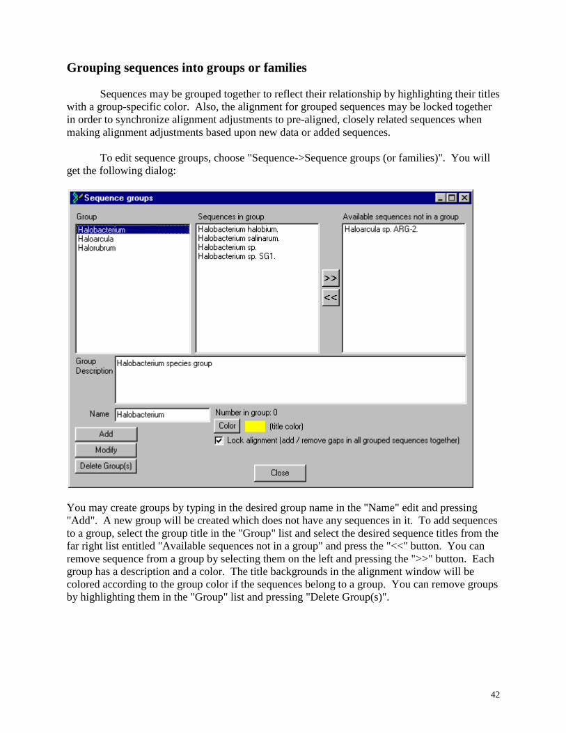
42
Grouping sequences into groups or families
Sequences may be grouped together to reflect their relationship by highlighting their titles
with a group-specific color. Also, the alignment for grouped sequences may be locked together
in order to synchronize alignment adjustments to pre-aligned, closely related sequences when
making alignment adjustments based upon new data or added sequences.
To edit sequence groups, choose "Sequence->Sequence groups (or families)". You will
get the following dialog:
You may create groups by typing in the desired group name in the "Name" edit and pressing
"Add". A new group will be created which does not have any sequences in it. To add sequences
to a group, select the group title in the "Group" list and select the desired sequence titles from the
far right list entitled "Available sequences not in a group" and press the "<<" button. You can
remove sequence from a group by selecting them on the left and pressing the ">>" button. Each
group has a description and a color. The title backgrounds in the alignment window will be
colored according to the group color if the sequences belong to a group. You can remove groups
by highlighting them in the "Group" list and pressing "Delete Group(s)".
43
Verbal confirmation of sequences
If you hand-type a small sequence into the single-sequence editor, for example a primer
sequence to be stored in a file and ordered for synthesis, it is sometimes helpful to have someone
read back the sequence for you as you verify on paper base by base as they read. If there is
nobody available to read your sequence to you, BioEdit will slowly read a sequence back from
within the single sequence editor, highlighting each base as it goes along (amino acid sequences
may be read as well).
To read a sequence back from within the single sequence editor, choose "Edit->Read Sequence
Back (Press escape to cancel)".
Note: This is only available from the single sequence editor. To open a sequence in the single
sequence editor, double-click on its title, or highlight its title and choose "Sequence->Edit
Sequence".
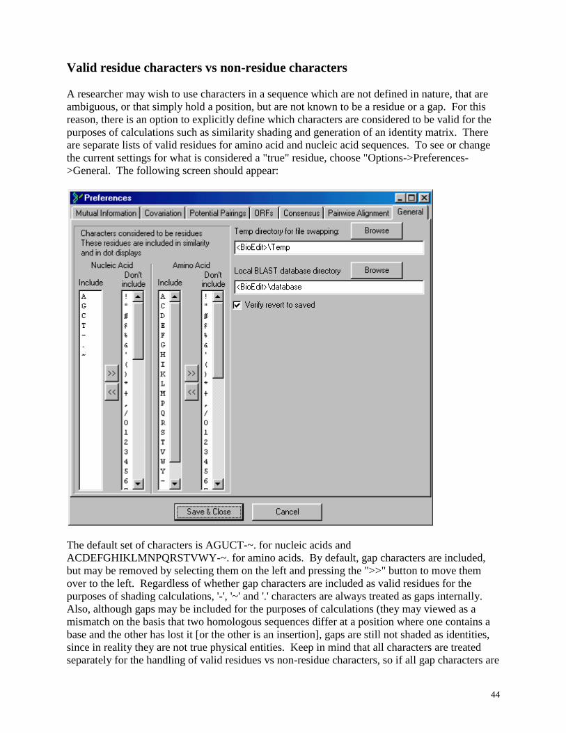
44
Valid residue characters vs non-residue characters
A researcher may wish to use characters in a sequence which are not defined in nature, that are
ambiguous, or that simply hold a position, but are not known to be a residue or a gap. For this
reason, there is an option to explicitly define which characters are considered to be valid for the
purposes of calculations such as similarity shading and generation of an identity matrix. There
are separate lists of valid residues for amino acid and nucleic acid sequences. To see or change
the current settings for what is considered a "true" residue, choose "Options->Preferences-
>General. The following screen should appear:
The default set of characters is AGUCT-~. for nucleic acids and
ACDEFGHIKLMNPQRSTVWY-~. for amino acids. By default, gap characters are included,
but may be removed by selecting them on the left and pressing the ">>" button to move them
over to the left. Regardless of whether gap characters are included as valid residues for the
purposes of shading calculations, '-', '~' and '.' characters are always treated as gaps internally.
Also, although gaps may be included for the purposes of calculations (they may viewed as a
mismatch on the basis that two homologous sequences differ at a position where one contains a
base and the other has lost it [or the other is an insertion], gaps are still not shaded as identities,
since in reality they are not true physical entities. Keep in mind that all characters are treated
separately for the handling of valid residues vs non-residue characters, so if all gap characters are
45
to be recognized (-, ~ and .), they all must be present in both the amino acid and nucleic acid lists
of valid residues.
Locking a sequence to prevent accidental edits
A sequence may be locked to prevent the ability to slide residues in that sequence or insert or
type over characters in the sequence either in the alignment window or the single sequence edit
window. If that sequence is grouped, hand alignment (by sliding only, not right mouse click
addition or deletion of gaps) of that sequence and all other sequences in the group is also
blocked if and only if the sequence group has group alignment locked. To lock a sequence, open
the sequence in the single sequence editor by either double-clicking on its title or by highlighting
its title and choosing "Sequence->Edit Sequence". In the edit box, check the
box, then press "Apply and Close".
Anchoring a column to protect aligned regions
It is sometimes useful to be able to lock a column of an alignment without having to
worry about accidentally pushing or pulling sequence over that position, although it may be off
of the current viewing screen. BioEdit therefore allows the anchoring of as many columns as
necessary to protect regions of an alignment that you don’t want to get messed up. To anchor a
column, depress the add / remove column anchors button ( ), then click the mouse over the
column you want anchored. To anchor an entire region, add a column anchor to each side of the
region you want protected. If you want to make sure that no alignment is possible in this region,
simply add an anchor to each side, unselect all sequence titles, select all the residues within the
region (highlight the region with the mouse by dragging the mouse on the ruler bar over the
region, then choose “Sequence->Gaps->Lock Gaps” to lock all the gaps in that region. That
region should be effectively locked until the anchors are removed (or the "“ignore anchors”
button is pressed down).
To remove an anchor, depress the button, then click over an existing anchor to remove it.
If you want to adjust the alignment in an anchored region, but don’t feel like resetting all of the
anchors, you may depress the “ignore column anchors” button ( ) and make your
adjustments. Be sure to hit the “ignore column anchors” button again after the adjustments are
finished to turn it off and make the anchors active again.
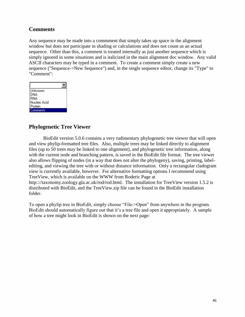
46
Comments
Any sequence may be made into a commment that simply takes up space in the alignment
window but does not participate in shading or calculations and does not count as an actual
sequence. Other than this, a comment is treated internally as just another sequence which is
simply ignored in some situations and is italicized in the main alignment doc window. Any valid
ASCII characters may be typed in a comment. To create a comment simply create a new
sequence ("Sequence->New Sequence") and, in the single sequence editor, change its "Type" to
"Comment":
Phylogenetic Tree Viewer
BioEdit version 5.0.6 contains a very rudimentary phylogenetic tree viewer that will open
and view phylip-formatted tree files. Also, multiple trees may be linked directly to alignment
files (up to 50 trees may be linked to one alignment), and phylogenetic tree information, along
with the current node and branching pattern, is saved in the BioEdit file format. The tree viewer
also allows flipping of nodes (in a way that does not alter the phylogeny), saving, printing, label-
editing, and viewing the tree with or without distance information. Only a rectangular cladogram
view is currently available, however. For alternative formatting options I recommend using
TreeView, which is available on the WWW from Roderic Page at
http:://taxonomy.zoology.gla.ac.uk/rod/rod.html. The installation for TreeView version 1.5.2 is
distributed with BioEdit, and the TreeView.zip file can be found in the BioEdit installation
folder.
To open a phylip tree in BioEdit, simply choose “File->Open” from anywhere in the program.
BioEdit should automatically figure out that it’s a tree file and open it appropriately. A sample
of how a tree might look in BioEdit is shown on the next page:
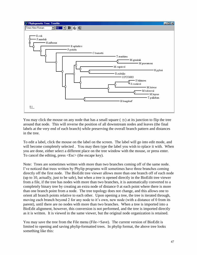
47
You may click the mouse on any node that has a small square ( ) at its junction to flip the tree
around that node. This will reverse the position of all downstream nodes and leaves (the final
labels at the very end of each branch) while preserving the overall branch pattern and distances
in the tree.
To edit a label, click the mouse on the label on the screen. The label will go into edit mode, and
will become completely selected . You may then type the label you wish to rplace it with. When
you are done, either select a different place on the tree window with the mouse, or press enter.
To cancel the editing, press <Esc> (the escape key).
Note: Trees are sometimes written with more than two branches coming off of the same node.
I’ve noticed that trees written by Phylip programs will sometimes have three branches coming
directly off the first node. The BioEdit tree viewer allows more than one branch off of each node
(up to 10, actually, just to be safe), but when a tree is opened directly in the BioEdit tree viewer
from a file, if the tree has nodes with more than two branches, it is automatically converted to a
completely binary tree by creating an extra node of distance 0 at each point where there is more
than one branch point from a node. The tree topology does not change, and this allows one to
orient all branch points relative to each other. Upon opening a tree, the tree is iterated through,
moving each branch beyond 2 for any node to it’s own, new node (with a distance of 0 from its
parent), until there are no nodes with more than two branches. When a tree is imported into a
BioEdit alignment, however, this conversion is not performed, and the tree is imported directly
as it is written. It is viewed in the same viewer, but the original node organization is retained.
You may save the tree from the File menu (File->Save). The current version of BioEdit is
limited to opening and saving phylip-formatted trees. In phylip format, the above tree looks
something like this:
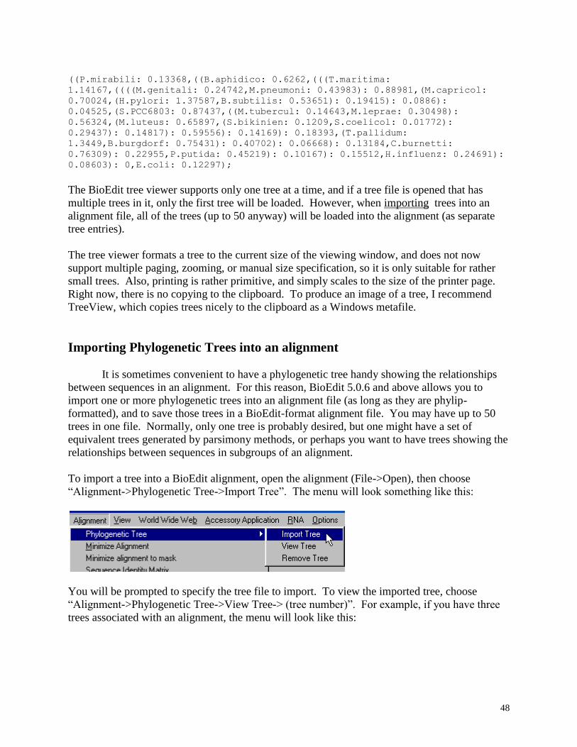
48
((P.mirabili: 0.13368,((B.aphidico: 0.6262,(((T.maritima:
1.14167,((((M.genitali: 0.24742,M.pneumoni: 0.43983): 0.88981,(M.capricol:
0.70024,(H.pylori: 1.37587,B.subtilis: 0.53651): 0.19415): 0.0886):
0.04525,(S.PCC6803: 0.87437,((M.tubercul: 0.14643,M.leprae: 0.30498):
0.56324,(M.luteus: 0.65897,(S.bikinien: 0.1209,S.coelicol: 0.01772):
0.29437): 0.14817): 0.59556): 0.14169): 0.18393,(T.pallidum:
1.3449,B.burgdorf: 0.75431): 0.40702): 0.06668): 0.13184,C.burnetti:
0.76309): 0.22955,P.putida: 0.45219): 0.10167): 0.15512,H.influenz: 0.24691):
0.08603): 0,E.coli: 0.12297);
The BioEdit tree viewer supports only one tree at a time, and if a tree file is opened that has
multiple trees in it, only the first tree will be loaded. However, when importing trees into an
alignment file, all of the trees (up to 50 anyway) will be loaded into the alignment (as separate
tree entries).
The tree viewer formats a tree to the current size of the viewing window, and does not now
support multiple paging, zooming, or manual size specification, so it is only suitable for rather
small trees. Also, printing is rather primitive, and simply scales to the size of the printer page.
Right now, there is no copying to the clipboard. To produce an image of a tree, I recommend
TreeView, which copies trees nicely to the clipboard as a Windows metafile.
Importing Phylogenetic Trees into an alignment
It is sometimes convenient to have a phylogenetic tree handy showing the relationships
between sequences in an alignment. For this reason, BioEdit 5.0.6 and above allows you to
import one or more phylogenetic trees into an alignment file (as long as they are phylip-
formatted), and to save those trees in a BioEdit-format alignment file. You may have up to 50
trees in one file. Normally, only one tree is probably desired, but one might have a set of
equivalent trees generated by parsimony methods, or perhaps you want to have trees showing the
relationships between sequences in subgroups of an alignment.
To import a tree into a BioEdit alignment, open the alignment (File->Open), then choose
“Alignment->Phylogenetic Tree->Import Tree”. The menu will look something like this:
You will be prompted to specify the tree file to import. To view the imported tree, choose
“Alignment->Phylogenetic Tree->View Tree-> (tree number)”. For example, if you have three
trees associated with an alignment, the menu will look like this:
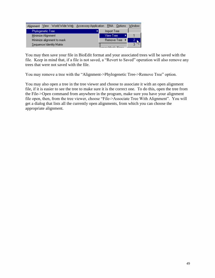
49
You may then save your file in BioEdit format and your associated trees will be saved with the
file. Keep in mind that, if a file is not saved, a “Revert to Saved” operation will also remove any
trees that were not saved with the file.
You may remove a tree with the “Alignment->Phylogenetic Tree->Remove Tree” option.
You may also open a tree in the tree viewer and choose to associate it with an open alignment
file, if it is easier to see the tree to make sure it is the correct one. To do this, open the tree from
the File->Open command from anywhere in the program, make sure you have your alignment
file open, then, from the tree viewer, choose “File->Associate Tree With Alignment”. You will
get a dialog that lists all the currently open alignments, from which you can choose the
appropriate alignment.
50
File formats
File formats read and written by BioEdit
BioEdit v5.0.0 reads and writes the following formats:
BioEdit
Genbank
Fasta
NBRF/PIR
Phylip 3.2 / 2
Phylip 4
In addition, BioEdit version 4.7.0 and above will read ABI model 377 autosequencer files.
The sequence is extracted and the trace is displayed on the screen and may also be printed in
color. BioEdit version 4.7.7 and above allows editing the editable sequence. The current
version also reads SCF trace files (versions 2 and 3), and ABI 373 and 3700 files.
BioEdit 4.7.7 and above also read both ClustalW and GCG-formatted files, but it does not
write them.
In addition to these formats, an external input/output filter (Don Gilbert’s ReadSeq) is provided,
allowing for the import and export of the following formats:
IG/Stanford
EMBL
GCG (single sequence only)
DNAStrider
Fitch
Zuker (import only)
Olsen (import only)
Plain or raw (single sequence only)
PIR/CODATA
MSF (multiple sequence format)
ASN.1 (NCBI)
PAUP/NEXUS
Documentation for the ReadSeq utility can be found in the file ReadSeq.txt in the /apps folder of
the BioEdit installation directory. Use of this utility within BioEdit is automatic when opening
sequences. If a file is opened which is not one of the formats read by BioEdit, you be prompted
to try to open it with ReadSeq. If ReadSeq can open it, it will be imported into BioEdit as a
GenBank file, otherwise it will be opened as text. To save a file in one of these formats, choose
File->Export->Sequence alignment from an open document.
51
BioEdit Project File Format
BioEdit provides a specialized binary alignment format for very fast opening and saving of large
alignment files (20 Mb+ file sizes -- even up to 100 Mb or larger). Reading and figuring out raw
text becomes very slow in large alignments of formats such as GenBank, where there is no
header telling the program how may sequences there are or how big they are.
The structure of a BioEdit Project file is as follows:
Header
1. offset 0x00000000: the string “**BioEdit Project File**” identifies the file as a BioEdit
Project file (first version).
2. The string “**BioEdit Project File02” at offset 0x00000000 identifies the file as version
2 of the BioEdit format (the current version). Previous versions of BioEdit will not read
the current BioEdit format, but BioEdit v5.0.0 or above will read the old BioEdit format.
3. offset 0x00000018: the number of sequences in the file.
4. offset 0x0000001C: the index of the mask sequence (if there is one).
5. offset 0x00000020: the index of the numbering mask (if there is one).
Offset 0x000000C8: The offsets for each sequence data structure.
Each sequence structure consists of a title, a sequence, the sequence type, and all of the same
GenBank fields included with a GenBank file in BioEdit. In addition, in BioEdit v5.0.0 or
above, graphical sequence annotations, sequence grouping information, consensus sequence
information, sequence locking status, and positional flags are saved. None of these latter
additions are saved in any of the other, standard, formats Each field is preceded by a long
integer specifying the length of the data, so each piece of data may be read from the file as a
single chunk, which allows a file to be read very quickly.
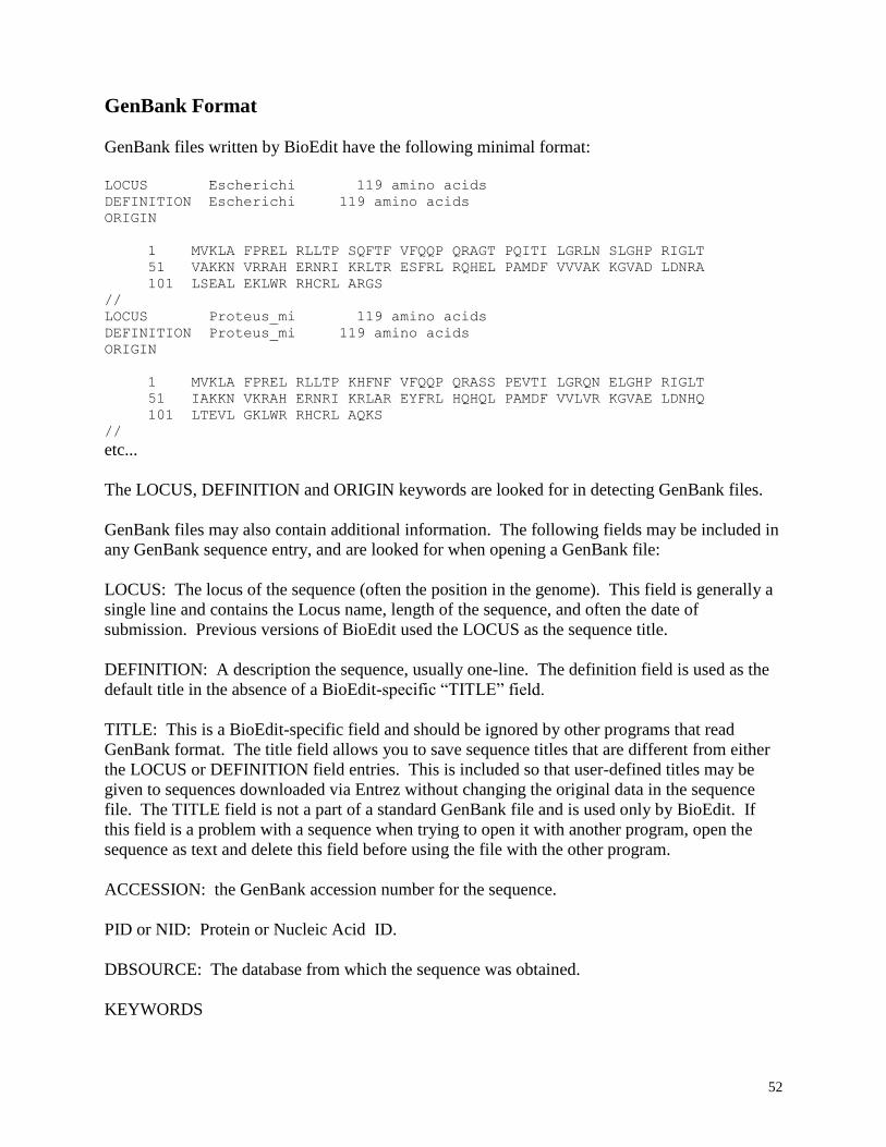
52
GenBank Format
GenBank files written by BioEdit have the following minimal format:
LOCUS Escherichi 119 amino acids
DEFINITION Escherichi 119 amino acids
ORIGIN
1 MVKLA FPREL RLLTP SQFTF VFQQP QRAGT PQITI LGRLN SLGHP RIGLT
51 VAKKN VRRAH ERNRI KRLTR ESFRL RQHEL PAMDF VVVAK KGVAD LDNRA
101 LSEAL EKLWR RHCRL ARGS
//
LOCUS Proteus_mi 119 amino acids
DEFINITION Proteus_mi 119 amino acids
ORIGIN
1 MVKLA FPREL RLLTP KHFNF VFQQP QRASS PEVTI LGRQN ELGHP RIGLT
51 IAKKN VKRAH ERNRI KRLAR EYFRL HQHQL PAMDF VVLVR KGVAE LDNHQ
101 LTEVL GKLWR RHCRL AQKS
//
etc...
The LOCUS, DEFINITION and ORIGIN keywords are looked for in detecting GenBank files.
GenBank files may also contain additional information. The following fields may be included in
any GenBank sequence entry, and are looked for when opening a GenBank file:
LOCUS: The locus of the sequence (often the position in the genome). This field is generally a
single line and contains the Locus name, length of the sequence, and often the date of
submission. Previous versions of BioEdit used the LOCUS as the sequence title.
DEFINITION: A description the sequence, usually one-line. The definition field is used as the
default title in the absence of a BioEdit-specific “TITLE” field.
TITLE: This is a BioEdit-specific field and should be ignored by other programs that read
GenBank format. The title field allows you to save sequence titles that are different from either
the LOCUS or DEFINITION field entries. This is included so that user-defined titles may be
given to sequences downloaded via Entrez without changing the original data in the sequence
file. The TITLE field is not a part of a standard GenBank file and is used only by BioEdit. If
this field is a problem with a sequence when trying to open it with another program, open the
sequence as text and delete this field before using the file with the other program.
ACCESSION: the GenBank accession number for the sequence.
PID or NID: Protein or Nucleic Acid ID.
DBSOURCE: The database from which the sequence was obtained.
KEYWORDS
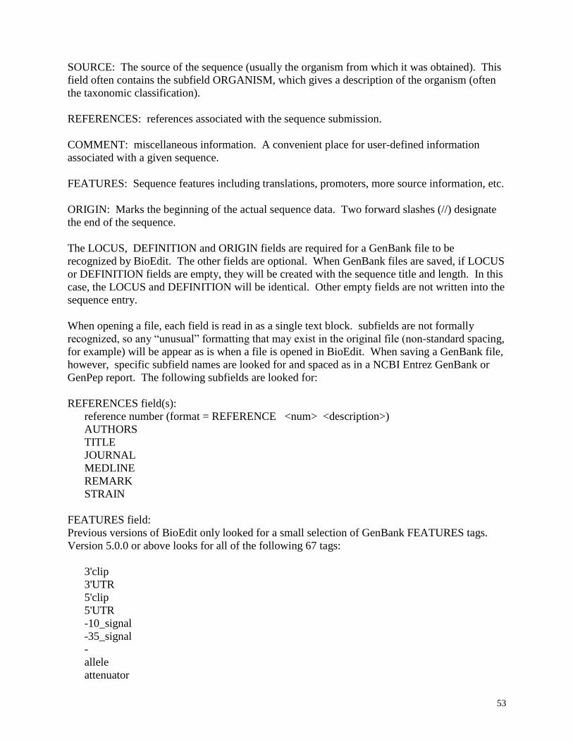
53
SOURCE: The source of the sequence (usually the organism from which it was obtained). This
field often contains the subfield ORGANISM, which gives a description of the organism (often
the taxonomic classification).
REFERENCES: references associated with the sequence submission.
COMMENT: miscellaneous information. A convenient place for user-defined information
associated with a given sequence.
FEATURES: Sequence features including translations, promoters, more source information, etc.
ORIGIN: Marks the beginning of the actual sequence data. Two forward slashes (//) designate
the end of the sequence.
The LOCUS, DEFINITION and ORIGIN fields are required for a GenBank file to be
recognized by BioEdit. The other fields are optional. When GenBank files are saved, if LOCUS
or DEFINITION fields are empty, they will be created with the sequence title and length. In this
case, the LOCUS and DEFINITION will be identical. Other empty fields are not written into the
sequence entry.
When opening a file, each field is read in as a single text block. subfields are not formally
recognized, so any “unusual” formatting that may exist in the original file (non-standard spacing,
for example) will be appear as is when a file is opened in BioEdit. When saving a GenBank file,
however, specific subfield names are looked for and spaced as in a NCBI Entrez GenBank or
GenPep report. The following subfields are looked for:
REFERENCES field(s):
reference number (format = REFERENCE <num> <description>)
AUTHORS
TITLE
JOURNAL
MEDLINE
REMARK
STRAIN
FEATURES field:
Previous versions of BioEdit only looked for a small selection of GenBank FEATURES tags.
Version 5.0.0 or above looks for all of the following 67 tags:
3'clip
3'UTR
5'clip
5'UTR
-10_signal
-35_signal
-
allele
attenuator
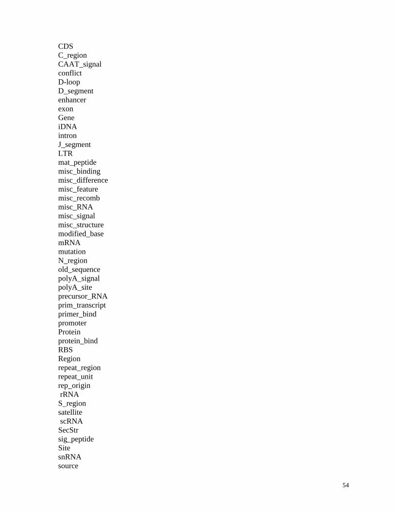
54
CDS
C_region
CAAT_signal
conflict
D-loop
D_segment
enhancer
exon
Gene
iDNA
intron
J_segment
LTR
mat_peptide
misc_binding
misc_difference
misc_feature
misc_recomb
misc_RNA
misc_signal
misc_structure
modified_base
mRNA
mutation
N_region
old_sequence
polyA_signal
polyA_site
precursor_RNA
prim_transcript
primer_bind
promoter
Protein
protein_bind
RBS
Region
repeat_region
repeat_unit
rep_origin
rRNA
S_region
satellite
scRNA
SecStr
sig_peptide
Site
snRNA
source
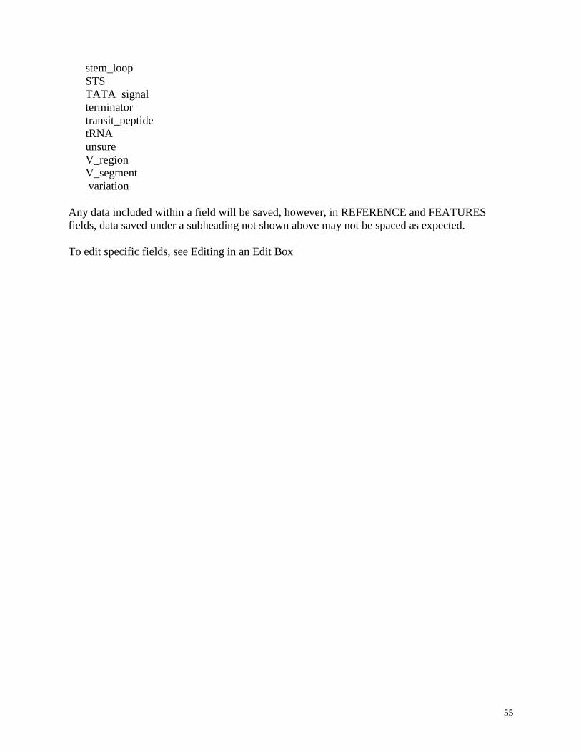
55
stem_loop
STS
TATA_signal
terminator
transit_peptide
tRNA
unsure
V_region
V_segment
variation
Any data included within a field will be saved, however, in REFERENCE and FEATURES
fields, data saved under a subheading not shown above may not be spaced as expected.
To edit specific fields, see Editing in an Edit Box
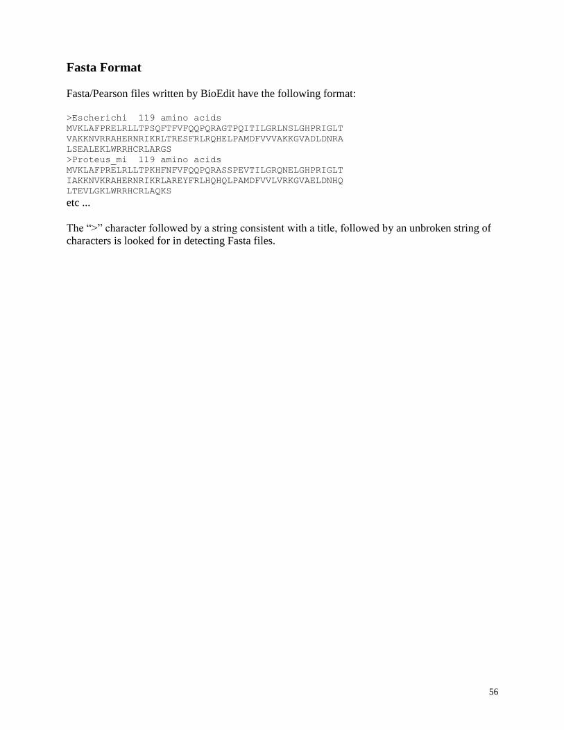
56
Fasta Format
Fasta/Pearson files written by BioEdit have the following format:
>Escherichi 119 amino acids
MVKLAFPRELRLLTPSQFTFVFQQPQRAGTPQITILGRLNSLGHPRIGLT
VAKKNVRRAHERNRIKRLTRESFRLRQHELPAMDFVVVAKKGVADLDNRA
LSEALEKLWRRHCRLARGS
>Proteus_mi 119 amino acids
MVKLAFPRELRLLTPKHFNFVFQQPQRASSPEVTILGRQNELGHPRIGLT
IAKKNVKRAHERNRIKRLAREYFRLHQHQLPAMDFVVLVRKGVAELDNHQ
LTEVLGKLWRRHCRLAQKS
etc ...
The “>” character followed by a string consistent with a title, followed by an unbroken string of
characters is looked for in detecting Fasta files.
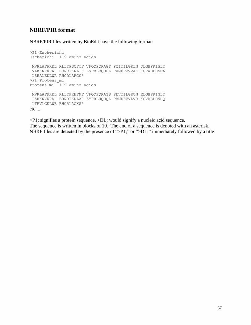
57
NBRF/PIR format
NBRF/PIR files written by BioEdit have the following format:
>P1;Escherichi
Escherichi 119 amino acids
MVKLAFPREL RLLTPSQFTF VFQQPQRAGT PQITILGRLN SLGHPRIGLT
VAKKNVRRAH ERNRIKRLTR ESFRLRQHEL PAMDFVVVAK KGVADLDNRA
LSEALEKLWR RHCRLARGS*
>P1;Proteus_mi
Proteus_mi 119 amino acids
MVKLAFPREL RLLTPKHFNF VFQQPQRASS PEVTILGRQN ELGHPRIGLT
IAKKNVKRAH ERNRIKRLAR EYFRLHQHQL PAMDFVVLVR KGVAELDNHQ
LTEVLGKLWR RHCRLAQKS*
etc ...
>P1; signifies a protein sequence, >DL; would signify a nucleic acid sequence.
The sequence is written in blocks of 10. The end of a sequence is denoted with an asterisk.
NBRF files are detected by the presence of “>P1;” or “>DL;” immediately followed by a title
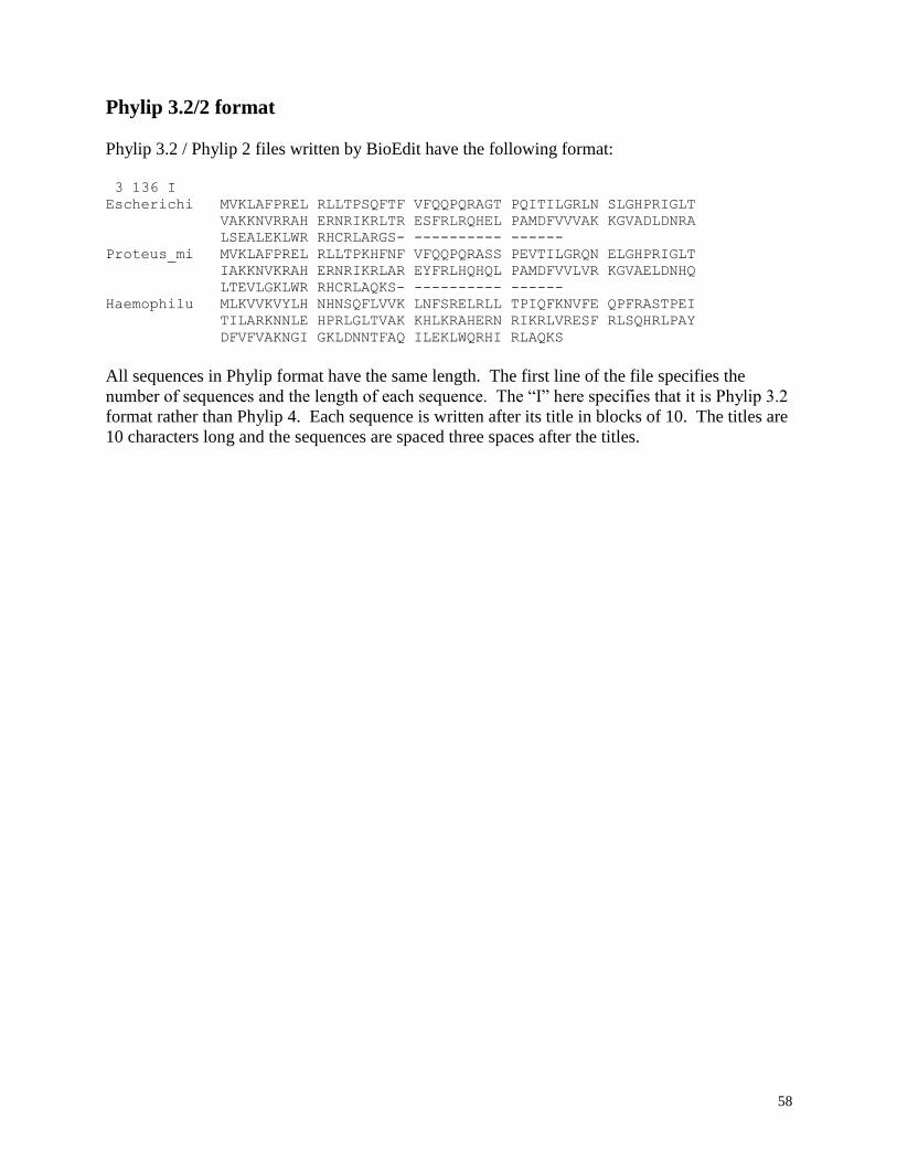
58
Phylip 3.2/2 format
Phylip 3.2 / Phylip 2 files written by BioEdit have the following format:
3 136 I
Escherichi MVKLAFPREL RLLTPSQFTF VFQQPQRAGT PQITILGRLN SLGHPRIGLT
VAKKNVRRAH ERNRIKRLTR ESFRLRQHEL PAMDFVVVAK KGVADLDNRA
LSEALEKLWR RHCRLARGS- ---------- ------
Proteus_mi MVKLAFPREL RLLTPKHFNF VFQQPQRASS PEVTILGRQN ELGHPRIGLT
IAKKNVKRAH ERNRIKRLAR EYFRLHQHQL PAMDFVVLVR KGVAELDNHQ
LTEVLGKLWR RHCRLAQKS- ---------- ------
Haemophilu MLKVVKVYLH NHNSQFLVVK LNFSRELRLL TPIQFKNVFE QPFRASTPEI
TILARKNNLE HPRLGLTVAK KHLKRAHERN RIKRLVRESF RLSQHRLPAY
DFVFVAKNGI GKLDNNTFAQ ILEKLWQRHI RLAQKS
All sequences in Phylip format have the same length. The first line of the file specifies the
number of sequences and the length of each sequence. The “I” here specifies that it is Phylip 3.2
format rather than Phylip 4. Each sequence is written after its title in blocks of 10. The titles are
10 characters long and the sequences are spaced three spaces after the titles.
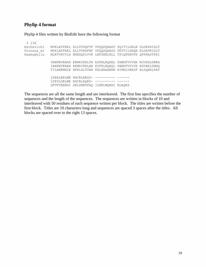
59
Phylip 4 format
Phylip 4 files written by BioEdit have the following format
3 136
Escherichi MVKLAFPREL RLLTPSQFTF VFQQPQRAGT PQITILGRLN SLGHPRIGLT
Proteus_mi MVKLAFPREL RLLTPKHFNF VFQQPQRASS PEVTILGRQN ELGHPRIGLT
Haemophilu MLKVVKVYLH NHNSQFLVVK LNFSRELRLL TPIQFKNVFE QPFRASTPEI
VAKKNVRRAH ERNRIKRLTR ESFRLRQHEL PAMDFVVVAK KGVADLDNRA
IAKKNVKRAH ERNRIKRLAR EYFRLHQHQL PAMDFVVLVR KGVAELDNHQ
TILARKNNLE HPRLGLTVAK KHLKRAHERN RIKRLVRESF RLSQHRLPAY
LSEALEKLWR RHCRLARGS- ---------- ------
LTEVLGKLWR RHCRLAQKS- ---------- ------
DFVFVAKNGI GKLDNNTFAQ ILEKLWQRHI RLAQKS
The sequences are all the same length and are interleaved. The first line specifies the number of
sequences and the length of the sequences. The sequences are written in blocks of 10 and
interleaved with 50 residues of each sequence written per block. The titles are written before the
first block. Titles are 10 characters long and sequences are spaced 3 spaces after the titles. All
blocks are spaced over to the right 13 spaces.
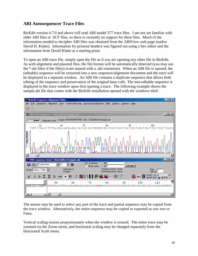
60
ABI Autosequencer Trace Files
BioEdit version 4.7.0 and above will read ABI model 377 trace files. I am not yet familiar with
older ABI files or .SCF files, so there is currently no support for these files. Much of the
information needed to decipher ABI files was obtained from the ABIView web page (author
David H. Klatte). Information for printout headers was figured out using a hex editor and the
information from David Klatte as a starting point.
To open an ABI trace file, simply open the file as if you are opening any other file in BioEdit.
As with alignment and plasmid files, the file format will be automatically detected (you may use
the *.abi filter if the file(s) is/are named with a .abi extension). When an ABI file is opened, the
(editable) sequence will be extracted into a new sequence/alignment document and the trace will
be displayed in a separate window. An ABI file contains a duplicate sequence that allows both
editing of the sequence and preservation of the original base-calls The non-editable sequence is
displayed in the trace window upon first opening a trace. The following example shows the
sample.abi file that comes with the BioEdit installation opened with the windows tiled:
The mouse may be used to select any part of the trace and partial sequence may be copied from
the trace window. Alternatively, the entire sequence may be copied or exported as raw text or
Fasta.
Vertical scaling resizes proportionately when the window is resized. The entire trace may be
zoomed via the Zoom menu, and horizontal scaling may be changed separately from the
Horizontal Scale menu.
61
To edit the sequence, you must first switch to the editable sequence by choosing View->Editable
sequence. Individual basecalls may be edited by highlighting the base with the mouse and typing
over it. Saving the edited sequence will not alter the non-editable sequence, and the non-editable
sequence may be viewed at any time by choosing View->Non-editable sequence. The non-
editable sequence is always shown by default upon first opening an ABI file. The editable
sequence, however, is the one extracted to a sequence document. The edited sequence may be
reverted at any time by choosing Edit->Revert edited to non-editable sequence.
You can view some of the relevant header information from the file by choosing File->info.
The trace and sequence may be reverse-complemented by choosing View->Reverse complement.
A printout of the trace looks similar to an ABI Prism printout. For most purposes, simply
choosing “Print” from the “File” menu will produce a formatted print of desirable scaling.
However horizontal and vertical scaling may be changed for printing via the “Print Scaling”
menu under the “File” menu. A set of presets may be chosen, or any exact scaling may be
specified (as %) by choosing “other”.
The picture on the following page is similar to what can be expected for page one of a printout of
the sample.abi file. A normal printout, however, will print at the ouput resolution of the printer
(the image in this document is a bitmap).
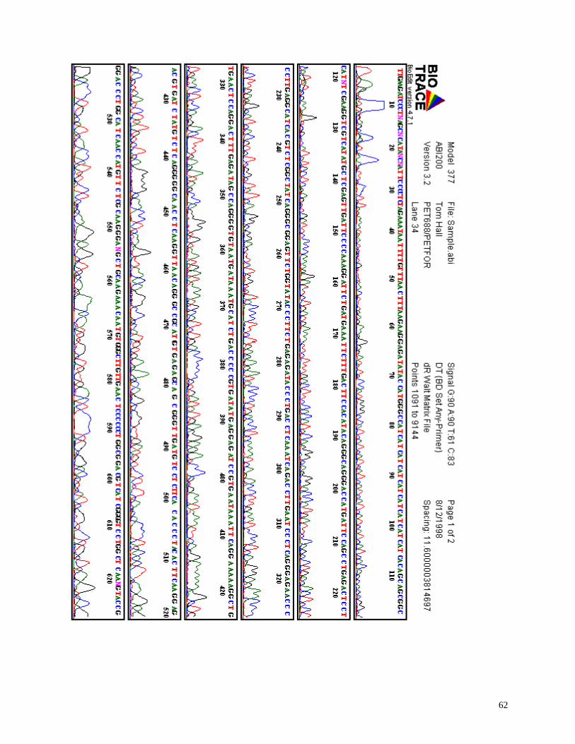
62
63
Saving sequence annotation information
BioEdit will save much of the information contained within a standard GenBank formatted file.
The following fields may be included in any GenBank or BioEdit file:
LOCUS
DEFINITION
TITLE (BioEdit specific -- not standard in GenBank format)
ACCESSION
PID or NID
DBSOURCE
KEYWORDS
SOURCE
REFERENCES
COMMENT
FEATURES
In addition to the text information retained in the "FEATURES" field, sequences may be
graphically annotated independently of these GenBank fields either manually or automatically
using the standard tags from the GenBank FEATURES field. Graphical annotation information,
however, will only be saved in BioEdit file format.
For a description of the above fields, see "GenBank file format".
For a description of the graphical sequence annotations, see "Graphical Feature Annotations".
Note that information other than sequence, title and length will only be saved in GenBank and
BioEdit format. It may be easiest to keep most sequence files in GenBank format and only use
other formats when a specific conversion is needed.
Reading Files saved with BioEdit with a Macintosh program
Macintosh computers use a different carriage return character than PC-compatibles. If you need
to use a file created in BioEdit with a Macintosh program such as SeqApp or DNA Strider, you
may need to first open the file with a word processor such as Microsoft Word or WordPerfect,
then save it again to produce the correct carriage returns. BioEdit will correctly read a file that
was created on a Macintosh or a UNIX machine.
64
Toggling between nucleotide and protein views
To control the way translation handles gaps , make sure the “Toggle Translation Control” option
is checked from the “View” menu, and that the “Force contiguous codons” and “Ignore gaps that
split codons” checkboxes are visible on the control bar of an alignment document.
When working with nucleotide sequences that code for proteins, BioEdit allows the toggling
back and forth between nucleotide and protein sequences, with each view reflecting any gaps
inserted or deleted in either view. The nucleotide information is retained when toggling back
from a protein view (it is not re-translated degenerately).
To switch back and forth between nucleotide and protein views of protein-encoding nucleic
acids, first trim the 5’ end of the sequence(s) to the start codon and make sure the coding region
is in frame 1. Then either select the sequences to toggle and choose “Toggle Translation” from
the Sequence” menu, or choose “Toggle Translation” from the “Alignment” menu (in which case
all sequences will be automatically selected and toggled). The sequences may be aligned in
either view. Additionally, if the protein view is Clustal-aligned, the underlying nucleotide
sequences will be updated with the proper gaps.
Note 1: When saving an alignment, if the sequences are toggled on the protein view, the
nucleotide sequences, not the proteins, are saved.
Note 2: This feature is only functional when the starting sequences are nucleic acid. If the
starting sequences are protein, then this feature does not do anything when chosen, because the
coding region of a protein cannot be known by examining the amino acid sequence alone. The
feature can be used on degenerate reverse translations by first reverse-translating the sequences,
then choosing this menu option.
Note 3: There are three available modes for handling gaps placed in nucleotide sequences
which either split codons internally or occur as singles or pairs. A gap in a protein sequence
will correspond to three gaps in the encoding nucleotide sequence. However, if a one or two
gaps are placed in a nucleotide sequence, or gaps are placed directly within a codon (in frame 1),
there is a problem. BioEdit handles this in one of three ways, depending upon the options
chosen:
To alter the options for translation toggling, the “Translation Toggle Control” option under the
“View” menu must be checked. When this menu item is checked, there will be two checkboxes
on the right side of the top panel of the alignment window. The available options are:
1. Force all gaps to occur in groups of three and to only occur between codon (not within
codons). In this mode, if a gap is introduced inside a codon, the nucleotides downstream are
shifted left until a full codon is produced. If this results in a single or double gap (or if one is
manually put between two codons), the gap is extended to three places to make a single amino
acid size gap. This will cause gap positions to automatically change if they are not introduced as
triplets between codons. It is easiest to simply align the sequences by their protein translations.
** This mode is active when the “Force contiguous codons” checkbox is checked.
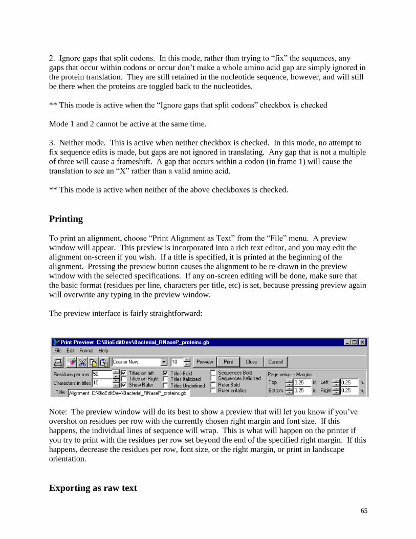
65
2. Ignore gaps that split codons. In this mode, rather than trying to “fix” the sequences, any
gaps that occur within codons or occur don’t make a whole amino acid gap are simply ignored in
the protein translation. They are still retained in the nucleotide sequence, however, and will still
be there when the proteins are toggled back to the nucleotides.
** This mode is active when the “Ignore gaps that split codons” checkbox is checked
Mode 1 and 2 cannot be active at the same time.
3. Neither mode. This is active when neither checkbox is checked. In this mode, no attempt to
fix sequence edits is made, but gaps are not ignored in translating. Any gap that is not a multiple
of three will cause a frameshift. A gap that occurs within a codon (in frame 1) will cause the
translation to see an “X” rather than a valid amino acid.
** This mode is active when neither of the above checkboxes is checked.
Printing
To print an alignment, choose “Print Alignment as Text” from the “File” menu. A preview
window will appear. This preview is incorporated into a rich text editor, and you may edit the
alignment on-screen if you wish. If a title is specified, it is printed at the beginning of the
alignment. Pressing the preview button causes the alignment to be re-drawn in the preview
window with the selected specifications. If any on-screen editing will be done, make sure that
the basic format (residues per line, characters per title, etc) is set, because pressing preview again
will overwrite any typing in the preview window.
The preview interface is fairly straightforward:
Note: The preview window will do its best to show a preview that will let you know if you’ve
overshot on residues per row with the currently chosen right margin and font size. If this
happens, the individual lines of sequence will wrap. This is what will happen on the printer if
you try to print with the residues per row set beyond the end of the specified right margin. If this
happens, decrease the residues per row, font size, or the right margin, or print in landscape
orientation.
Exporting as raw text
66
BioEdit provides an easy function for converting alignments into properly spaced raw text files.
To export the alignment as a raw text file (no formatting), select the “Save As ...” option from
the “File” menu and choose “Text Files” from the “Save as type” options in the save dialog.
You will get a dialog that asks for the number of residues per line (by tens) and the number of
characters per title to save:
Exporting as Rich Text
An alignment shaded for identities and similarities may be exported in rich text format,
preserving the residue highlighting as long as the file is viewed with Word 97 or newer or
another word processor that supports highlighting in rich text. The alignment is shaded
according to the current settings for shaded graphic views, and exporting in this format may also
be done directly from the shaded graphic view form. To export an alignment as rich text directly
from a document, choose File->Export->Rich text with current shaded view settings.
Shaded graphic view of alignment
For a presentation of the alignment showing identities and similarities shaded, select the titles
for the sequences you want to include, then choose “Graphic View” from the “File” menu of an
open document. This is similar to the print preview, but allows for the shading of identical and
similar residues in the alignment, and allows you to show any subset of the alignment.
The following options are currently offered:
Variable threshold percentage for shading residues (one threshold for both identities and
similarities)
Show or hide ruler
Show or hide titles on the left and right of sequence data
Show or hide position numbers on the left and right
Variable number of residues per line (by tens -- 20 to 2000)
Variable number of characters per title (5 to 30)
Titles may be bolded, italicized and/or underlined
Sequences may be italicized and/or bolded
A choice of scoring matrices is available
Fonts: Any font can be used and will spaced approximately correctly. However, some fonts
look odd in this view (most, actually, are spaced too wide because the widest character must
be accommodated), and typeset fonts work best. For greater control over the font, choose
“Character Font” from the “Font” menu.
Colors for background of page, identities and similarities and colors for non-identical,
identical and similar residue characters.
A title may be added which will be placed at the beginning of each page. In this release, this
creates a problem if the alignment requires more than one page, so it is best to leave the title
field blank.
Alignment may be drawn in the standard color table colors (to allow printing of the
alignment in color).

67
Shading according to identity and similarity (threshold defined by “Threshold (%) for
shading” on control panel) may be done with the user defined colors on the control panel, or
with current alignment color table colors.
Lines of sequence may be blocked into groups of 10 (like a Phylip file) or printed as
continuous, unbroken lines.
Translations may be shown below nucleic acid sequences in either 3-letter or one-letter codes
Shaded alignments may be exported as rich text documents which preserve colored
highlighting (Word 97 or above, or equivalent, is required to display highlighting in rich
text).
When certain changes are made to the current view, the “Redraw” button must be pressed for the
changes to take place on the screen. Many changes are automatically updated.
To change colors, either double-click on the labeled, colored box, or press the small button to the
left of it.
To copy a page to the clipboard for pasting into another application, choose “Copy” form the
“Edit” menu. A page may be copied as a bitmap or an Enhanced Windows Metafile (EMF).
Copying as a metafile allows for pasting directly into an application such as PowerPoint for
inclusion of a shaded alignment in a slide presentation, or into a page layout program for creation
of a publication figure. A metafile offers the advantage of being a vectored graphic (the graphics
are defined by formula/code rather than pixels such as in a bitmap) which can take advantage of
the full resolution of the output device. At this time, only an entire page can be copied. A later
version may offer annotation and selection capabilities, if there is demand for this.
Multiple pages are supported for long alignments, however, this is a serious problem with this
version of BioEdit. Currently, a page is defined vertically by the page height in inches specified
by the user in the graphic view window. When vertically scrolling through the graphic view, the
current page is shown in the upper right of the form. When the end of one page is reached, the
next page is drawn in its place. There is no continuing view from page to page, which can make
viewing page transitions on-screen very tedious. Also, some image-editing is required to
produce an image figure of an alignment that takes more than one page. Currently, it is easiest if
the alignment can be made to fit on one page. The height of a page can be set to up to 100
inches, but this will take an enormous amount of memory and is not recommended (each page is
a bitmapped image). To create an image longer than a piece of paper, you can increase the page
height and copy the image to the clipboard. On a slow computer, there is a delay as each new
page is drawn.
Previous versions of BioEdit determined the page size only vertically. The current version
calculates the specified page settings (from the print setup and the margin and page size settings)
and will clip the graphical image if it runs over the right side of the page. This should
correspond rather closely (may not always be perfect) with what will print on the currently
chosen printer with the current settings. Also, margins are now shown in the graphic view to
reflect a fairly accurate print preview for each page.
The following are two shaded views of a ClustalW alignment of bacteriorhodopsin protein
sequences from representative halophilic Archaea:
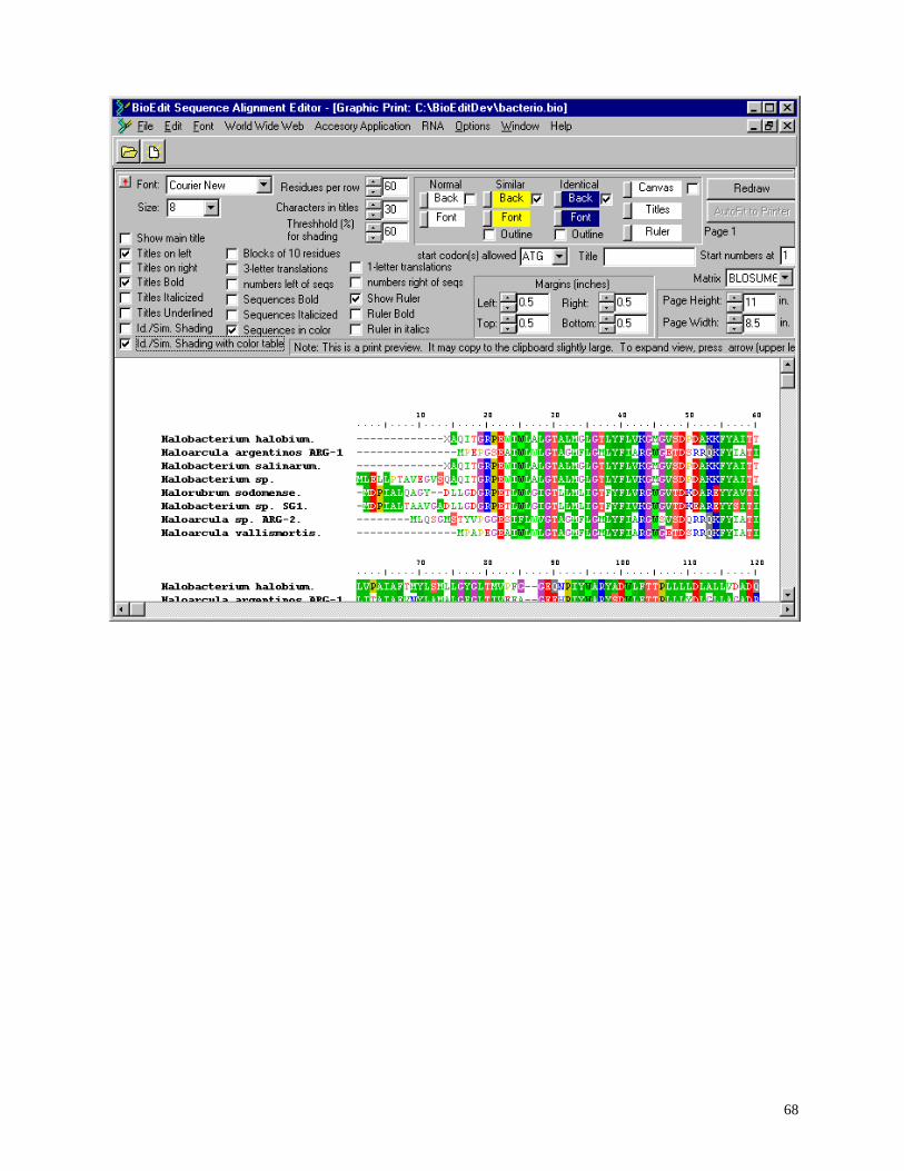
68
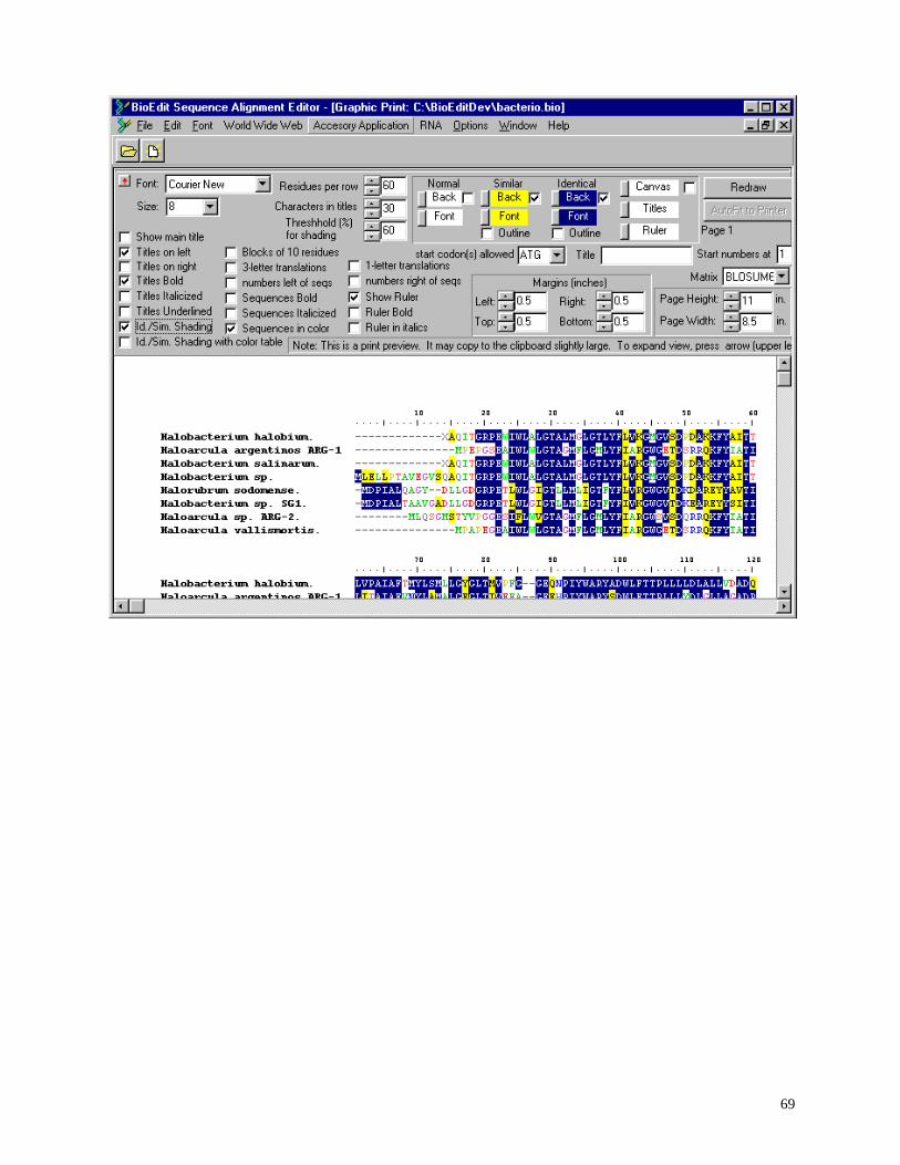
69

70
Information-based shading in the alignment window
The following view shows an information-based shaded view of an alignment of 75 16S rRNA
sequences from methanogenic Archaea. The region shown was picked by an
entropy/information-based search for conserved regions.
Compare this view to the split-window view below it showing the same alignment with this
region compared to a less well-conserved region (on the next page).
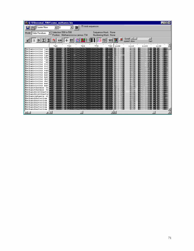
71
72
Restriction Maps
BioEdit offers two ways to generate restriction maps of nucleic acid sequences. An internal
restriction map utility allows generation of maps for sequences up to 65,536 nucleotides. It has
only really been tested up to about 35 Kb, and it takes a while on a slower computer for a large
sequence. You can also link directly to WebCutter restriction mapping via the World Wide
Web.
WebCutter: Highlight the title of the sequence you wish to map and choose “Auto-fed
WebCutter Restriction Mapping” from the “World Wide Web” menu.
BioEdit: Highlight the title of the sequence you wish to map and choose “Restriction Map”
from the “Sequence” menu. An interface window will appear with the following options:
-- Display Map: Display or omit a full map of the sequence and the complementary strand
showing the cut positions of each enzyme. Default: yes
-- Alphabetical by name: Display a list of all enzymes that cut, their recognition sequences,
frequency of cutting, and all positions (5' end starting at 1). Default: yes
-- Numeric by position: A list of all positions that are cut, in increasing order, and the enzymes
that cut there. Enzyme cut positions are defined at the cut site, rather than the start of the
recognition sequence (e.g.. if a BamHI site (G'GATC_C) started at position 1476, the cut
position would be reported as 1477 -- where it actually cuts). Default: no
-- List of unique sites: List of enzymes that cut only once in the entire sequence. Default: no
-- Enzymes that cut five or fewer times. Default: yes
-- Summary table of frequencies: A table of all enzymes currently selected and the number of
times they cut in the sequence. Default: no
-- Enzymes that do not cut. Default: yes
-- 4-base cutters: You may choose to omit enzymes that cut at a 4-base recognition sequence. To
include these enzymes, the box must be checked. Default: no (don’t include 4-base cutters).
-- 5-base cutters: Same as 4-base cutters.
-- Enzymes with degenerate recognition sequences: Many restriction enzymes recognize
sequences loosely. For example, AccI recognizes the sequence “GT'mk_AC”, where ‘m’ can be
A or C and ‘k’ can be G or T. You may wish to exclude these on occasion. Default: include
these.
-- Large recognition sites: Often for cloning, only the common 6-base recognizing enzymes are
used. If you do not want a map cluttered with extra information, uncheck this box (as well as 4-
base and 5-base cutters).
-- All Isoschizomers: The enzyme list file used is the GCG-format file available from ReBase.
Several enzymes are in this file which cut the same recognition sequence of other enzymes in the
file. To show only one enzyme for a particular recognition site, uncheck this box
(Default=unchecked). If this option is chosen, the map will be very large. Isoschizomers for all
enzymes which you choose to include may be examined by viewing the enzyme table from the
mapping interface (press the “View Current Enzyme Table” button).
-- Three frame translation: Shows a translation along the sequence as shown in the alignment
(assumed to be in the 5' to 3' orientation left to right).
-- Translation of complement: A three-frame translation of the complementary strand running the
opposite direction.
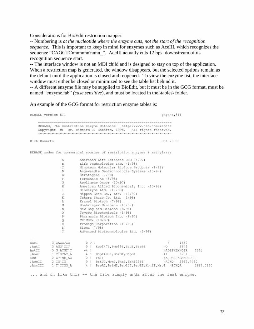
73
Considerations for BioEdit restriction mapper.
-- Numbering is at the nucleotide where the enzyme cuts, not the start of the recognition
sequence. This is important to keep in mind for enzymes such as AceIII, which recognizes the
sequence “CAGCTCnnnnnnn'nnnn_”. AceIII actually cuts 12 bps. downstream of its
recognition sequence start.
-- The interface window is not an MDI child and is designed to stay on top of the application.
When a restriction map is generated, the window disappears, but the selected options remain as
the default until the application is closed and reopened. To view the enzyme list, the interface
window must either be closed or minimized to see the table list behind it.
-- A different enzyme file may be supplied to BioEdit, but it must be in the GCG format, must be
named “enzyme.tab” (case sensitive), and must be located in the \tables\ folder.
An example of the GCG format for restriction enzyme tables is:
REBASE version 811 gcgenz.811
=-=-=-=-=-=-=-=-=-=-=-=-=-=-=-=-=-=-=-=-=-=-=-=-=-=-=-=-=-=-=-=-=-=
REBASE, The Restriction Enzyme Database http://www.neb.com/rebase
Copyright (c) Dr. Richard J. Roberts, 1998. All rights reserved.
=-=-=-=-=-=-=-=-=-=-=-=-=-=-=-=-=-=-=-=-=-=-=-=-=-=-=-=-=-=-=-=-=-=
Rich Roberts Oct 28 98
REBASE codes for commercial sources of restriction enzymes & methylases
A Amersham Life Sciences-USB (4/97)
B Life Technologies Inc. (1/98)
C Minotech Molecular Biology Products (1/98)
D Angewandte Gentechnologie Systeme (10/97)
E Stratagene (1/98)
F Fermentas AB (5/98)
G Appligene Oncor (10/97)
H American Allied Biochemical, Inc. (10/98)
I SibEnzyme Ltd. (10/98)
J Nippon Gene Co., Ltd. (10/97)
K Takara Shuzo Co. Ltd. (1/98)
L Kramel Biotech (7/98)
M Boehringer-Mannheim (10/97)
N New England BioLabs (8/98)
O Toyobo Biochemicals (1/98)
P Pharmacia Biotech Inc. (8/97)
Q CHIMERx (10/97)
R Promega Corporation (10/98)
S Sigma (7/98)
T Advanced Biotechnologies Ltd. (3/98)
..
AarI 3 CACCTGC 0 ? ! > 1667
;AatI 3 AGG'CCT 0 ! Eco147I,Pme55I,StuI,SseBI >O 6643
AatII 5 G_ACGT'C -4 ! >ADEFKLMNOPR 6643
;AauI 1 T'GTAC_A 4 ! Bsp1407I,BsrGI,SspBI >I 6251
AccI 2 GT'mk_AC 2 ! FblI >ABDEGJKLMNOPQRS
;AccII 2 CG'CG 0 ! BstUI,MvnI,ThaI,Bsh1236I >AJKQ 3992,7430
;AccIII 1 T'CCGG_A 4 ! BseAI,BsiMI,Bsp13I,BspEI,Kpn2I,MroI >EJKQR 3994,5140
... and on like this -- the file simply ends after the last enzyme.
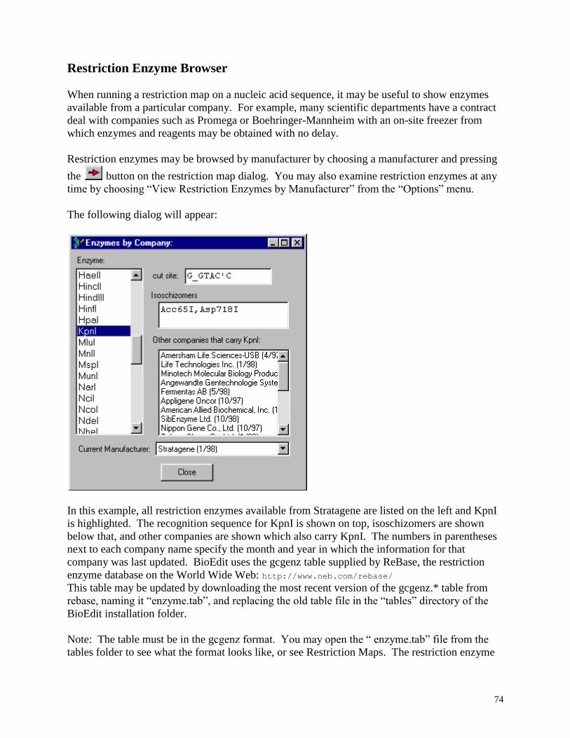
74
Restriction Enzyme Browser
When running a restriction map on a nucleic acid sequence, it may be useful to show enzymes
available from a particular company. For example, many scientific departments have a contract
deal with companies such as Promega or Boehringer-Mannheim with an on-site freezer from
which enzymes and reagents may be obtained with no delay.
Restriction enzymes may be browsed by manufacturer by choosing a manufacturer and pressing
the button on the restriction map dialog. You may also examine restriction enzymes at any
time by choosing “View Restriction Enzymes by Manufacturer” from the “Options” menu.
The following dialog will appear:
In this example, all restriction enzymes available from Stratagene are listed on the left and KpnI
is highlighted. The recognition sequence for KpnI is shown on top, isoschizomers are shown
below that, and other companies are shown which also carry KpnI. The numbers in parentheses
next to each company name specify the month and year in which the information for that
company was last updated. BioEdit uses the gcgenz table supplied by ReBase, the restriction
enzyme database on the World Wide Web: http://www.neb.com/rebase/
This table may be updated by downloading the most recent version of the gcgenz.* table from
rebase, naming it “enzyme.tab”, and replacing the old table file in the “tables” directory of the
BioEdit installation folder.
Note: The table must be in the gcgenz format. You may open the “ enzyme.tab” file from the
tables folder to see what the format looks like, or see Restriction Maps. The restriction enzyme
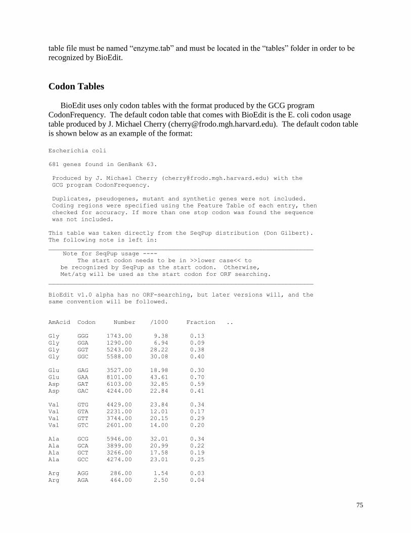
75
table file must be named “enzyme.tab” and must be located in the “tables” folder in order to be
recognized by BioEdit.
Codon Tables
BioEdit uses only codon tables with the format produced by the GCG program
CodonFrequency. The default codon table that comes with BioEdit is the E. coli codon usage
table produced by J. Michael Cherry ([email protected]). The default codon table
is shown below as an example of the format:
Escherichia coli
681 genes found in GenBank 63.
Produced by J. Michael Cherry ([email protected]) with the
GCG program CodonFrequency.
Duplicates, pseudogenes, mutant and synthetic genes were not included.
Coding regions were specified using the Feature Table of each entry, then
checked for accuracy. If more than one stop codon was found the sequence
was not included.
This table was taken directly from the SeqPup distribution (Don Gilbert).
The following note is left in:
_________________________________________________________________________
Note for SeqPup usage ----
The start codon needs to be in >>lower case<< to
be recognized by SeqPup as the start codon. Otherwise,
Met/atg will be used as the start codon for ORF searching.
_________________________________________________________________________
BioEdit v1.0 alpha has no ORF-searching, but later versions will, and the
same convention will be followed.
AmAcid Codon Number /1000 Fraction ..
Gly GGG 1743.00 9.38 0.13
Gly GGA 1290.00 6.94 0.09
Gly GGT 5243.00 28.22 0.38
Gly GGC 5588.00 30.08 0.40
Glu GAG 3527.00 18.98 0.30
Glu GAA 8101.00 43.61 0.70
Asp GAT 6103.00 32.85 0.59
Asp GAC 4244.00 22.84 0.41
Val GTG 4429.00 23.84 0.34
Val GTA 2231.00 12.01 0.17
Val GTT 3744.00 20.15 0.29
Val GTC 2601.00 14.00 0.20
Ala GCG 5946.00 32.01 0.34
Ala GCA 3899.00 20.99 0.22
Ala GCT 3266.00 17.58 0.19
Ala GCC 4274.00 23.01 0.25
Arg AGG 286.00 1.54 0.03
Arg AGA 464.00 2.50 0.04
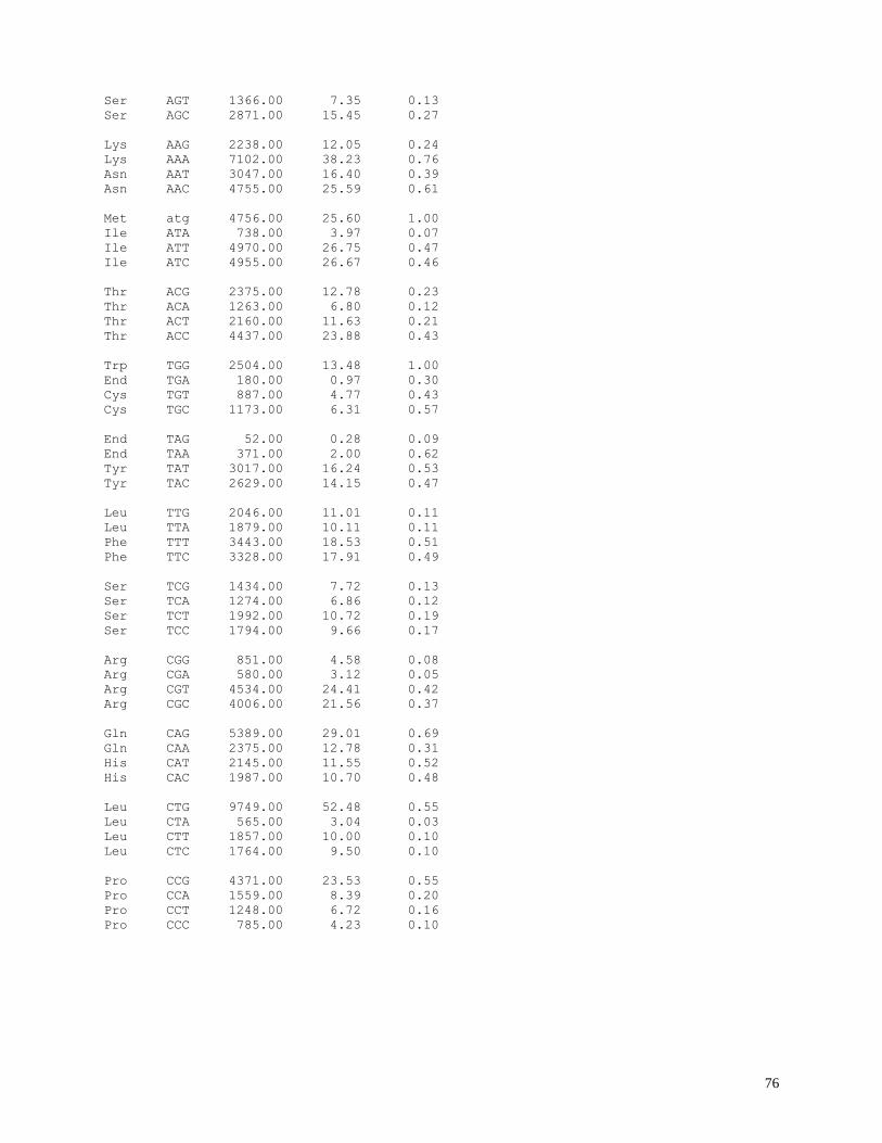
76
Ser AGT 1366.00 7.35 0.13
Ser AGC 2871.00 15.45 0.27
Lys AAG 2238.00 12.05 0.24
Lys AAA 7102.00 38.23 0.76
Asn AAT 3047.00 16.40 0.39
Asn AAC 4755.00 25.59 0.61
Met atg 4756.00 25.60 1.00
Ile ATA 738.00 3.97 0.07
Ile ATT 4970.00 26.75 0.47
Ile ATC 4955.00 26.67 0.46
Thr ACG 2375.00 12.78 0.23
Thr ACA 1263.00 6.80 0.12
Thr ACT 2160.00 11.63 0.21
Thr ACC 4437.00 23.88 0.43
Trp TGG 2504.00 13.48 1.00
End TGA 180.00 0.97 0.30
Cys TGT 887.00 4.77 0.43
Cys TGC 1173.00 6.31 0.57
End TAG 52.00 0.28 0.09
End TAA 371.00 2.00 0.62
Tyr TAT 3017.00 16.24 0.53
Tyr TAC 2629.00 14.15 0.47
Leu TTG 2046.00 11.01 0.11
Leu TTA 1879.00 10.11 0.11
Phe TTT 3443.00 18.53 0.51
Phe TTC 3328.00 17.91 0.49
Ser TCG 1434.00 7.72 0.13
Ser TCA 1274.00 6.86 0.12
Ser TCT 1992.00 10.72 0.19
Ser TCC 1794.00 9.66 0.17
Arg CGG 851.00 4.58 0.08
Arg CGA 580.00 3.12 0.05
Arg CGT 4534.00 24.41 0.42
Arg CGC 4006.00 21.56 0.37
Gln CAG 5389.00 29.01 0.69
Gln CAA 2375.00 12.78 0.31
His CAT 2145.00 11.55 0.52
His CAC 1987.00 10.70 0.48
Leu CTG 9749.00 52.48 0.55
Leu CTA 565.00 3.04 0.03
Leu CTT 1857.00 10.00 0.10
Leu CTC 1764.00 9.50 0.10
Pro CCG 4371.00 23.53 0.55
Pro CCA 1559.00 8.39 0.20
Pro CCT 1248.00 6.72 0.16
Pro CCC 785.00 4.23 0.10
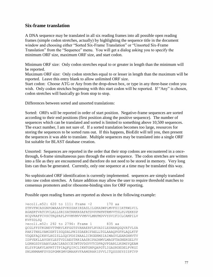
77
Six-frame translation
A DNA sequence may be translated in all six reading frames into all possible open reading
frames (simple codon stretches, actually) by highlighting the sequence title in the document
window and choosing either “Sorted Six-Frame Translation” or “Unsorted Six-Frame
Translation” from the “Sequence” menu. You will get a dialog asking you to specify the
minimum ORF size, maximum ORF size, and start codon.
Minimum ORF size: Only codon stretches equal to or greater in length than the minimum will
be reported.
Maximum ORF size: Only codon stretches equal to or lesser in length than the maximum will be
reported. Leave this entry blank to allow unlimited ORF size.
Start codon: Choose ATG or Any from the drop-down box, or type in any three-base codon you
wish. Only codon stretches beginning with this start codon will be reported. If “Any” is chosen,
codon stretches will basically go from stop to stop.
Differences between sorted and unsorted translations:
Sorted: ORFs will be reported in order of start position. Negative-frame sequences are sorted
according to their end positions (first position along the positive sequence). The number of
sequences which can be translated and sorted is limited to something above 10,500 sequences.
The exact number, I am not sure of. If a sorted translation becomes too large, resources for
storing the sequences to be sorted runs out. If this happens, BioEdit will tell you, then present
the sequences it was able to translate. Multiple sequences may be translated into a single ORF
list suitable for BLAST database creation.
Unsorted: Sequences are reported in the order that their stop codons are encountered in a once-
through, 6-frame simultaneous pass through the entire sequence. The codon stretches are written
into a file as they are encountered and therefore do not need to be stored in memory. Very long
lists can thus be generated. Currently, only one sequence at a time may be translated this way.
No sophisticated ORF identification is currently implemented. sequences are simply translated
into raw codon stretches. A future addition may allow the user to require threshold matches to
consensus promoters and/or ribosome-binding sites for ORF reporting.
Possible open reading frames are reported as shown in the following example:
>ecoli.m52: 620 to 111: Frame -2 170 aa
STKVFNCASGNPGWAAASPVKSSAKIRSASLILGKASWPLMVFSIIATRWLVIL
AGAERTVATCPCLALLSRISATRRKRSAFATDVPPNFNTRMVVTSLPLVEKKSP
HCQVRAFFCVSCTRQPAPLPVVMVMVVVMVVLMRFMDVVYSVIFICLCAMPILV
KVFSDLSQ
>ecoli.m52: 292 to 2796: Frame 1 835 aa
QCGLFFSTKGNEVTTMRVLKFGGTSVANAERFLRVADILESNARQGQVATVLSA
PAKITNHLVAMIEKTISGQDALPNISDAERIFAELLTGLAAAQPGFPLAQLKTF
VDQEFAQIKHVLHGISLLGQCPDSINAALICRGEKMSIAIMAGVLEARGHNVTV
IDPVEKLLAVGHYLESTVDIAESTRRIAASRIPADHMVLMAGFTAGNEKGELVV
LGRNGSDYSAAVLAACLRADCCEIWTDVDGVYTCDPRQVPDARLLKSMSYQEAM
ELSYFGAKVLHPRTITPIAQFQIPCLIKNTGNPQAPGTLIGASRDEDELPVKGI
SNLNNMAMFSVSGPGMKGMVGMAARVFAAMSRARISVVLITQSSSEYSISFCVP
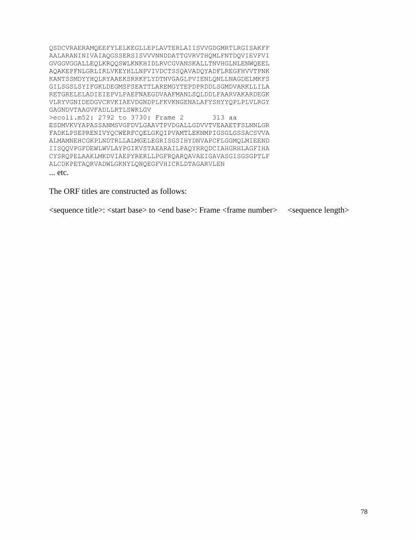
78
QSDCVRAERAMQEEFYLELKEGLLEPLAVTERLAIISVVGDGMRTLRGISAKFF
AALARANINIVAIAQGSSERSISVVVNNDDATTGVRVTHQMLFNTDQVIEVFVI
GVGGVGGALLEQLKRQQSWLKNKHIDLRVCGVANSKALLTNVHGLNLENWQEEL
AQAKEPFNLGRLIRLVKEYHLLNPVIVDCTSSQAVADQYADFLREGFHVVTPNK
KANTSSMDYYHQLRYAAEKSRRKFLYDTNVGAGLPVIENLQNLLNAGDELMKFS
GILSGSLSYIFGKLDEGMSFSEATTLAREMGYTEPDPRDDLSGMDVARKLLILA
RETGRELELADIEIEPVLPAEFNAEGDVAAFMANLSQLDDLFAARVAKARDEGK
VLRYVGNIDEDGVCRVKIAEVDGNDPLFKVKNGENALAFYSHYYQPLPLVLRGY
GAGNDVTAAGVFADLLRTLSWKLGV
>ecoli.m52: 2792 to 3730: Frame 2 313 aa
ESDMVKVYAPASSANMSVGFDVLGAAVTPVDGALLGDVVTVEAAETFSLNNLGR
FADKLPSEPRENIVYQCWERFCQELGKQIPVAMTLEKNMPIGSGLGSSACSVVA
ALMAMNEHCGKPLNDTRLLALMGELEGRISGSIHYDNVAPCFLGGMQLMIEEND
IISQQVPGFDEWLWVLAYPGIKVSTAEARAILPAQYRRQDCIAHGRHLAGFIHA
CYSRQPELAAKLMKDVIAEPYRERLLPGFRQARQAVAEIGAVASGISGSGPTLF
ALCDKPETAQRVADWLGKNYLQNQEGFVHICRLDTAGARVLEN ... etc.
The ORF titles are constructed as follows:
<sequence title>: <start base> to <end base>: Frame <frame number> <sequence length>
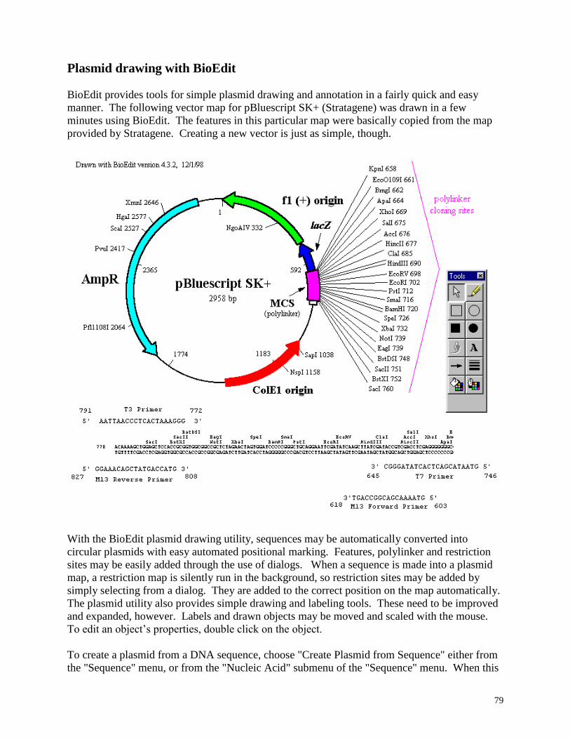
79
Plasmid drawing with BioEdit
BioEdit provides tools for simple plasmid drawing and annotation in a fairly quick and easy
manner. The following vector map for pBluescript SK+ (Stratagene) was drawn in a few
minutes using BioEdit. The features in this particular map were basically copied from the map
provided by Stratagene. Creating a new vector is just as simple, though.
With the BioEdit plasmid drawing utility, sequences may be automatically converted into
circular plasmids with easy automated positional marking. Features, polylinker and restriction
sites may be easily added through the use of dialogs. When a sequence is made into a plasmid
map, a restriction map is silently run in the background, so restriction sites may be added by
simply selecting from a dialog. They are added to the correct position on the map automatically.
The plasmid utility also provides simple drawing and labeling tools. These need to be improved
and expanded, however. Labels and drawn objects may be moved and scaled with the mouse.
To edit an object’s properties, double click on the object.
To create a plasmid from a DNA sequence, choose "Create Plasmid from Sequence" either from
the "Sequence" menu, or from the "Nucleic Acid" submenu of the "Sequence" menu. When this
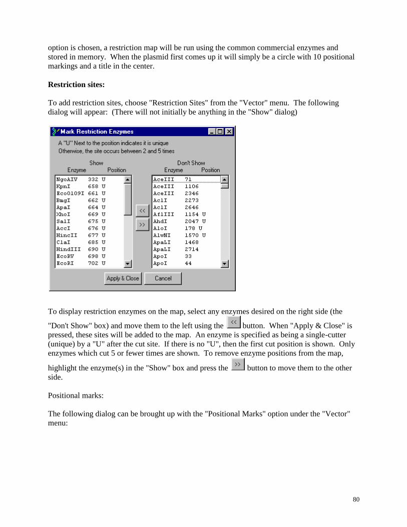
80
option is chosen, a restriction map will be run using the common commercial enzymes and
stored in memory. When the plasmid first comes up it will simply be a circle with 10 positional
markings and a title in the center.
Restriction sites:
To add restriction sites, choose "Restriction Sites" from the "Vector" menu. The following
dialog will appear: (There will not initially be anything in the "Show" dialog)
To display restriction enzymes on the map, select any enzymes desired on the right side (the
"Don't Show" box) and move them to the left using the button. When "Apply & Close" is
pressed, these sites will be added to the map. An enzyme is specified as being a single-cutter
(unique) by a "U" after the cut site. If there is no "U", then the first cut position is shown. Only
enzymes which cut 5 or fewer times are shown. To remove enzyme positions from the map,
highlight the enzyme(s) in the "Show" box and press the button to move them to the other
side.
Positional marks:
The following dialog can be brought up with the "Positional Marks" option under the "Vector"
menu:
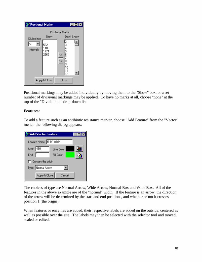
81
Positional markings may be added individually by moving them to the "Show" box, or a set
number of divisional markings may be applied. To have no marks at all, choose "none" at the
top of the "Divide into:" drop-down list.
Features:
To add a feature such as an antibiotic resistance marker, choose "Add Feature" from the "Vector"
menu. the following dialog appears:
The choices of type are Normal Arrow, Wide Arrow, Normal Box and Wide Box. All of the
features in the above example are of the "normal" width. If the feature is an arrow, the direction
of the arrow will be determined by the start and end positions, and whether or not it crosses
position 1 (the origin).
When features or enzymes are added, their respective labels are added on the outside, centered as
well as possible over the site. The labels may then be selected with the selector tool and moved,
scaled or edited.
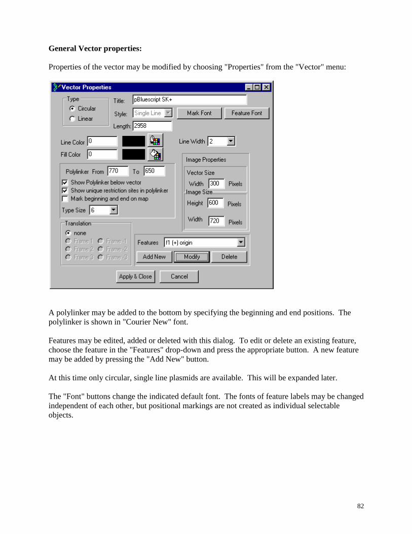
82
General Vector properties:
Properties of the vector may be modified by choosing "Properties" from the "Vector" menu:
A polylinker may be added to the bottom by specifying the beginning and end positions. The
polylinker is shown in "Courier New" font.
Features may be edited, added or deleted with this dialog. To edit or delete an existing feature,
choose the feature in the "Features" drop-down and press the appropriate button. A new feature
may be added by pressing the "Add New" button.
At this time only circular, single line plasmids are available. This will be expanded later.
The "Font" buttons change the indicated default font. The fonts of feature labels may be changed
independent of each other, but positional markings are not created as individual selectable
objects.
83
Drawing tools:
Very simple drawing tools are available which behave more or less like standard drawing tools
in most programs. The order of objects may be changed in the "Arrange" menu, and objects may
be grouped and ungrouped from the "Arrange" menu.
Note: Scaling grouped objects does not work well, as the objects are scaled independently of
each other.
To edit an object's properties, double-click on the object, or select the object and choose "Object
Properties" from the "Edit" menu.
Cut / Copy / Paste:
When an object(s) is copied in the plasmid utility, a structure is copied into memory for the use
of BioEdit, and a bitmap of the object or objects is copied to the clipboard. Objects may
therefore be pasted into other applications as bitmap images.
Printing:
When printing, the map is drawn to the printer at the printer's resolution to avoid the pixellation
that occurs with a screen-resolution bitmap. The print interface is not very advanced, however.
A left margin and top margin may be specified in the "Print Setup" dialog (from the "File" menu)
At this time there is no support for scaling output to the printer to defined print dimensions. The
size of the printed figure is determined by the ratio of printer resolution to screen resolution. The
full width of a screen set at 800 x 600 resolution corresponds to roughly 8.3 inches, which is
pretty close to the width of a normal paper page (8.5 inches). The plasmid itself scales slightly
small on the printer, and I’m currently trying to figure out why. The size relative to an 800 x 600
resolution screen is fairly close, however.
Moving the vector:
The vector may be moved around the page by first selecting it with the mouse (a dotted box will
be drawn around it to indicate it is selected), then dragging it with the mouse to its new location.
All of the labels and objects on the page will be moved accordingly.
84
Searching functions
The following search options are available under the Edit menu. These functions were never
originally conceived very well and have evolved sort of sloppily. Searching functionality is
lacking in BioEdit at this time and is in need of improvement.
Simple search: Find and Find Next
This is a very simple search function and needs to be improved. The menu option for
simple searching is found under Edit->Find. A standard search dialog is presented which allows
for searching of exact text strings (either case sensitive or insensitive) within selected sequences.
The search is always performed downwards from the beginning of the document, and only
includes sequences whose titles are selected (the search is performed only upon the sequences,
and does not include titles). When the text is found, the first instance encountered is highlighted
in the document window. The current search position is remembered. To continue the search to
find the next instance, select Edit->Find Again (F3, by default). If Edit->Find is chosen again,
the search position is reset to the beginning of the document.
Find in Titles and Find in Next Title
To highlight all titles containing specific text, choose Edit->Find in Titles. To highlight
the next title (either up or down) containing specific text, choose Edit->Find in Next Title. The
search is started at the last selected title in the specified direction.
Find Next ORF
When searching for ORFs, only sequences with selected titles are searched, and the search
begins after the last selected nucleotide. To search, choose Edit->Find Next ORF, or Sequence-
>Nucleic Acid->Find Next ORF. The search is performed according to the parameters specified
in the ORFs page of the preferences dialog. When an ORF is found, the sequence is highlighted
in the document window.
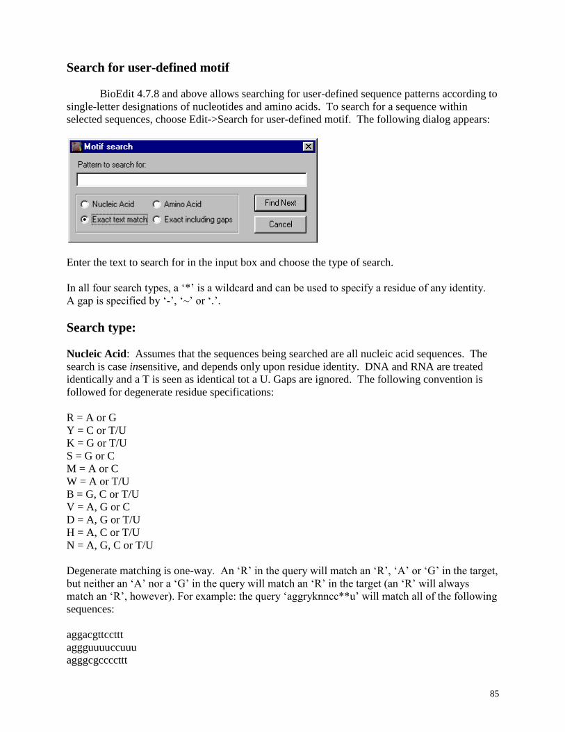
85
Search for user-defined motif
BioEdit 4.7.8 and above allows searching for user-defined sequence patterns according to
single-letter designations of nucleotides and amino acids. To search for a sequence within
selected sequences, choose Edit->Search for user-defined motif. The following dialog appears:
Enter the text to search for in the input box and choose the type of search.
In all four search types, a ‘*’ is a wildcard and can be used to specify a residue of any identity.
A gap is specified by ‘-’, ‘~’ or ‘.’.
Search type:
Nucleic Acid: Assumes that the sequences being searched are all nucleic acid sequences. The
search is case insensitive, and depends only upon residue identity. DNA and RNA are treated
identically and a T is seen as identical tot a U. Gaps are ignored. The following convention is
followed for degenerate residue specifications:
R = A or G
Y = C or T/U
K = G or T/U
S = G or C
M = A or C
W = A or T/U
B = G, C or T/U
V = A, G or C
D = A, G or T/U
H = A, C or T/U
N = A, G, C or T/U
Degenerate matching is one-way. An ‘R’ in the query will match an ‘R’, ‘A’ or ‘G’ in the target,
but neither an ‘A’ nor a ‘G’ in the query will match an ‘R’ in the target (an ‘R’ will always
match an ‘R’, however). For example: the query ‘aggryknncc**u’ will match all of the following
sequences:
aggacgttccttt
aggguuuuccuuu
agggcgccccttt
86
Amino Acid: Assumes that the sequences being searched are all amino acid sequences. The
search is case insensitive, and depends only upon residue identity. Gaps are ignored. The
following convention is followed for degenerate residue specifications:
X = any of the twenty standard amino acids
B = D or N
Z = E or Q
Like for nucleic acids, degenerate matching is one-way. A ‘B’ in the query will match a ‘B’, ‘D’
or ‘N’ in the target, but neither a ‘D’ nor a ‘N’ in the query will match an ‘B’ in the target (a ‘B’
will always match an ‘B’, however).
Standard one-letter amino acid codes are as follows:
A = Ala = alanine
C = Cys = cysteine
D = Asp = aspartate
E = Glu = glutamate
F = Phe = phenylalanine
G = Gly = glycine
H = His = histidine
I = Ile = isoleucine
K = Lys = lysine
L = leu = leucine
M = Met = methionine
N = Asn = asparagine
P = Pro = proline
Q = Gln = glutamine
R = Arg = arginine
S = Ser = serine
T = Thr = threonine
V = Val = valine
W = Trp = tryptophan
Y = Tyr = tyrosine
Exact text match:
A case insensitive search is performed, however, gaps (‘-’, ‘~’ or ‘.’) are ignored and ‘*’
represents any character. Note that a ‘T’ and a ‘U’ are different, even if the sequence type is
nucleic acid, and no degenerate identities are considered.

87
Exact including gaps:
Like an exact text match, but gaps are not ignored. A gap is still a ‘-’, ‘~’ or ‘.’, however, and
the search does not have to exactly specify the gap character present. A ‘*’ is still a wildcard in
this search and may be used to specifiy a character of any identity.
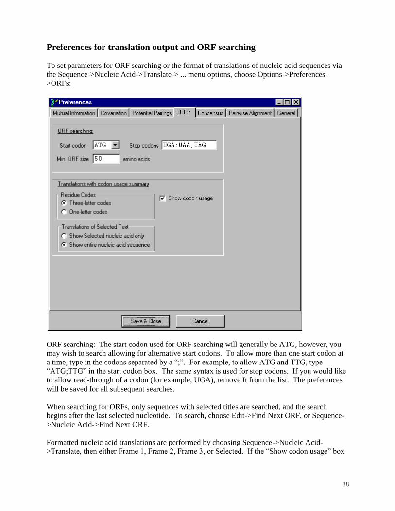
88
Preferences for translation output and ORF searching
To set parameters for ORF searching or the format of translations of nucleic acid sequences via
the Sequence->Nucleic Acid->Translate-> ... menu options, choose Options->Preferences-
>ORFs:
ORF searching: The start codon used for ORF searching will generally be ATG, however, you
may wish to search allowing for alternative start codons. To allow more than one start codon at
a time, type in the codons separated by a “;”. For example, to allow ATG and TTG, type
“ATG;TTG” in the start codon box. The same syntax is used for stop codons. If you would like
to allow read-through of a codon (for example, UGA), remove It from the list. The preferences
will be saved for all subsequent searches.
When searching for ORFs, only sequences with selected titles are searched, and the search
begins after the last selected nucleotide. To search, choose Edit->Find Next ORF, or Sequence-
>Nucleic Acid->Find Next ORF.
Formatted nucleic acid translations are performed by choosing Sequence->Nucleic Acid-
>Translate, then either Frame 1, Frame 2, Frame 3, or Selected. If the “Show codon usage” box
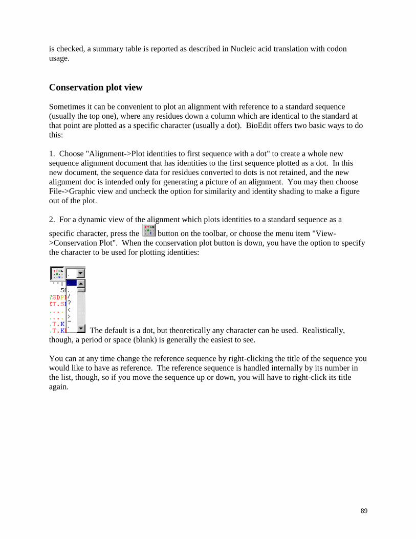
89
is checked, a summary table is reported as described in Nucleic acid translation with codon
usage.
Conservation plot view
Sometimes it can be convenient to plot an alignment with reference to a standard sequence
(usually the top one), where any residues down a column which are identical to the standard at
that point are plotted as a specific character (usually a dot). BioEdit offers two basic ways to do
this:
1. Choose "Alignment->Plot identities to first sequence with a dot" to create a whole new
sequence alignment document that has identities to the first sequence plotted as a dot. In this
new document, the sequence data for residues converted to dots is not retained, and the new
alignment doc is intended only for generating a picture of an alignment. You may then choose
File->Graphic view and uncheck the option for similarity and identity shading to make a figure
out of the plot.
2. For a dynamic view of the alignment which plots identities to a standard sequence as a
specific character, press the button on the toolbar, or choose the menu item "View-
>Conservation Plot". When the conservation plot button is down, you have the option to specify
the character to be used for plotting identities:
The default is a dot, but theoretically any character can be used. Realistically,
though, a period or space (blank) is generally the easiest to see.
You can at any time change the reference sequence by right-clicking the title of the sequence you
would like to have as reference. The reference sequence is handled internally by its number in
the list, though, so if you move the sequence up or down, you will have to right-click its title
again.
90
Basic Analysis Tools
BioEdit comes with a small (and somewhat uncoordinated) set of analysis functions and tools,
which are the focus of the rest of the docuemntation. Analysis features are split into two
categories:
1. External, independent programs which are written by other authors and are either distributed
with BioEdit or may be obtained from an outside source and can be run from the BioEdit
interface. BioEdit offers a somewhat general command line generator that may be
configured through a graphical interface to launch external analysis programs and feed
sequence data to them to facilitate an easier analysis environment from a single interface.
2. Functions which are built directly into BioEdit.
External Accessories
Installing TreeView:
TreeView is a phylogenetic tree viewing program written by Roderic D.M. Page. Previous
versions of BioEdit included a distribution of the TreeView executable and supporting libraries
in the apps folder. At the request of the author full TreeView installation is now distributed with
BioEdit. This installation is contained within the file called TreeView.zip.
To install TreeView, unzip the file to a temporary directory, then run the program called
"setup.exe" which will be created. TreeView will install itself on your system.
To configure TreeView to run through the accessory apps menu of BioEdit, choose
Add/Remove/Modify an Accessory Application from the Accessory Application menu. In the
"Name of Accessory" box, type “TreeView”. Press "Specify" next to the “Program” Box and
browse to the new location for the TreeView.exe program. Check the box called “Prompt for
input file”. In the “General Description” box, type “TreeView version 1.5.2. Copyright Roderic
D.M. Page, 1998. [email protected]. http://www.taxonomy.zoology.gla.ac.uk/rod/rod.html”
without any carriage returns. Then press “Add / Modify” at the bottom of the dialog. Upon
closing the window, you will be prompted to have BioEdit close and restart. For more
information on installing accessory applications, see Configuring and Using External
Applications.
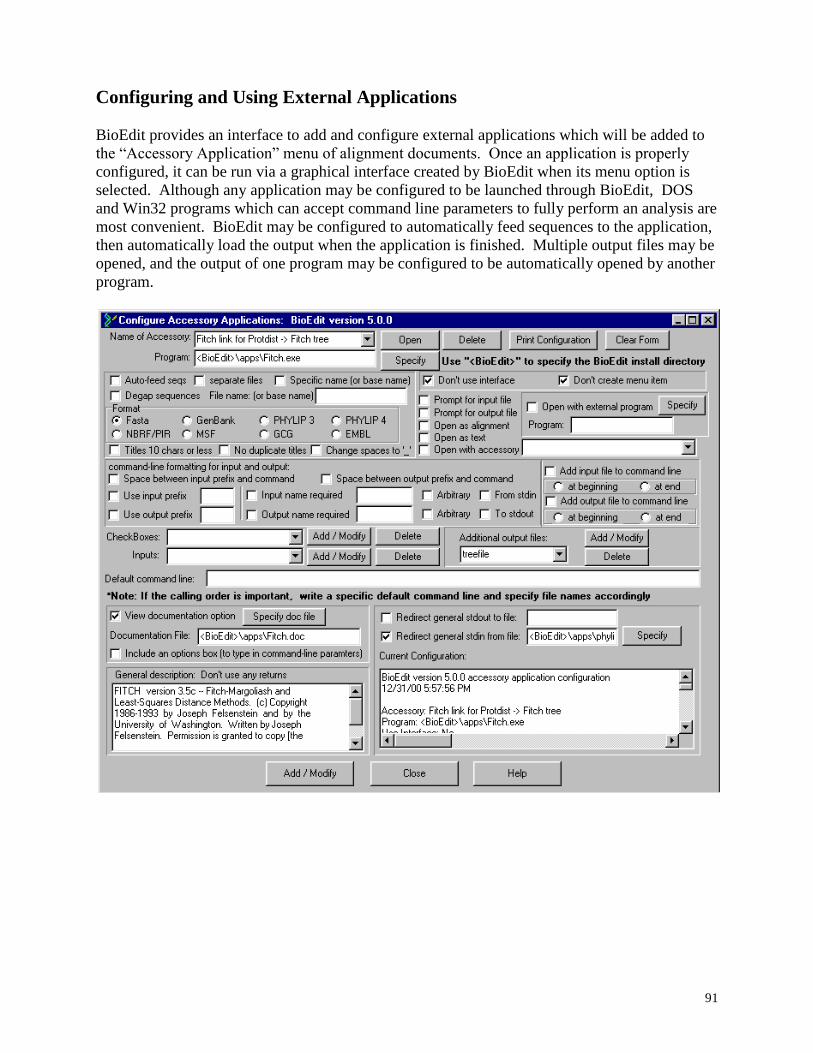
91
Configuring and Using External Applications
BioEdit provides an interface to add and configure external applications which will be added to
the “Accessory Application” menu of alignment documents. Once an application is properly
configured, it can be run via a graphical interface created by BioEdit when its menu option is
selected. Although any application may be configured to be launched through BioEdit, DOS
and Win32 programs which can accept command line parameters to fully perform an analysis are
most convenient. BioEdit may be configured to automatically feed sequences to the application,
then automatically load the output when the application is finished. Multiple output files may be
opened, and the output of one program may be configured to be automatically opened by another
program.
92
Adding and configuring a new application
BioEdit v2.0 and later offers a graphical interface for configuring external applications to be run
from a BioEdit alignment document. Unfortunately, there is no way to do this without knowing
how to run the application independently of BioEdit. A few programs come with the BioEdit
installation and are configured already. Permission has been granted by Joe Felsenstein to use
PHYLIP programs with BioEdit (as long as no money changes hands). Permission has also been
obtained from Roderic D.M. Page to distribute TreeView. TreeView is no longer pre-
configured, however. At the request of the author, BioEdit now comes with the TreeView install
package, which is extracted into the main installation folder upon installing BioEdit. For more
information, see Installing TreeView.
To add a new application to be included in the “Accessory Applications” menu, choose “Add /
Modify / Remove an Accessory Application” from the “Accessory Applications” menu.
There are several settings which must be specified for an accessory to be run successfully
through BioEdit. Many settings will not be required for many applications and each
configuration will be different, as programs are written differently by different people. One must
know how to run the program via a command line in order to configure BioEdit to run the
program. Refer to the documentation of your accessory application to learn how to run it before
trying to configure it as an accessory. The following options are present in the configuration
interface. Only the first two are universally required for all applications.
Name of Accessory: This is the name that will appear in the “Accessory Applications”
menu. This can be any name you want. It is recommended to keep it relatively short,
however, as it will be a menu option in all alignment documents.
Program: The absolute or relative path to the program, including the program name (usually
an .exe file, but could be a .com or a .bat file). To specify the path relative to the BioEdit
installation directory, specify the main installation directory as “<BioEdit>“ (not case
sensitive). For example, an application named “MyApp.exe” might be placed in the “apps”
directory. To allow the whole BioEdit directory to be moved without causing a problem with
finding the application, specify the path as “<BioEdit>\apps\MyApp.exe”. (Note: do not
include the quote marks). Alternatively, if the absolute path will be specified, you may
browse the disk to find the application by pressing “Specify”.
Automatically feed sequences to App: If the program analyzes sequence or alignment data
(such as ClustalW or certain PHYLIP programs), you may choose to have the sequences
automatically fed to the application. This is one of the most useful benefits of running the
program directly from an alignment editor. An application that takes only one or several
sequences may be done this way also, as BioEdit will only feed selected sequences at runtime
(if no sequences are selected, they will all be selected automatically).
Specific File name required (for auto-fed sequence data): Some applications expect a
specific input file name. For example, the PHYLIP programs all expect to process a file
called “infile”. If this is the case, check this box and enter the expected name in the “File
name” input box. Don’t include a path, since the file will be automatically saved to the
directory containing the application.
Degap sequences: Some applications require alignment data (such as DNAml, Protdist,
DNAdist, etc.) and gaps will be included in the input. Other programs (e.g. search programs
93
such as BLAST) may take simple sequence data rather than alignment data. In these cases,
gaps must be removed or they will be viewed as residues.
Format (for auto-fed sequences): Eight file formats are available for auto-feeding alignment
/ sequence data to programs: (if you have an application that requires a different format, you
may have to configure the application to take a certain file name, choose not to auto-feed the
sequences, and convert the file to the correct format before running the program -- or simply
run the program separately. If it would very convenient to have it run through BioEdit,
simply email me at [email protected] with file format name and specifications and it
would be a minor thing to write an export filter and add it to the accessory applications
method of BioEdit. If you need this, feel free to email me and I will mail back with an
address where the new copy of the program may be picked up and when (or if I can’t for
some reason, I will mail back and tell you that). Currently available formats are:
Fasta
GenBank
PHYLIP 2 / 3.2 (PHYLIP 3)
PHYLIP 4
NBRF/PIR
MSF (via ReadSeq.exe: Don Gilbert’s sequence conversion filter).
GCG (via ReadSeq.exe)
EMBL (via ReadSeq)
Prompt for input file: you may want to be prompted at runtime for an input file. BioEdit will
produce an open file dialog. The file name will be fed to the external program.
You may want BioEdit to prompt you at runtime to specify an output file name to feed to the
program.
Open as alignment: The main output of the program may be opened as a new alignment
document. (By default, there is expected to be one main output file, however, this is often
not the case, and additional output files may be specified in the box titled “Additional output
files:” -- this entry could be left blank and a single output could be specified as an additional
output. Functionally, this would make no difference).
Open as text. If the output is a text data file, it may be opened as text in the BioEdit rich text
editor.
Open with external program: Perhaps the program exports tabular or matrix data that you
would like to view in a spreadsheet program such as Microsoft Excel. You may specify any
external program to be launched and open the output automatically. You may browse the
disk by pressing “Specify”. You may also specify a path relative to the BioEdit installation
directory with “<BioEdit>“.
Note: An output file may be opened as a new alignment, as text and by an external
program all at the same time if you want.
Use input prefix: Some programs expect a specific prefix at the command line to specify the
input file, output file, the input of specific parameters, or all of these things. Other programs
may expect the input, output and parameters simply typed in a specific order. If you program
requires a prefix to specify the input file, check this box and enter the prefix exactly in the
associated edit box. Note: If the prefix and the file name will be separated by a space, type
that space after the prefix when configuring the application. For example, one application
may expect to see “-i inputFile” while another may expect “input=inputFile”. Depending on
how the applications are written, the first one may not work if the space is not included, and
the second one may not work if a space is included.
94
Use output prefix: Same as input prefix.
Input name required: Some applications require that an input file name be specified in the
command line (e.g. ClustalW). Others may expect a specific file name which therefore is not
specified at the command line (e.g. PHYLIP programs). If the application expects to be
given the name of the input file at the command line, check this option.
Output name required: Same as “Input name required”
Input or Output name arbitrary (check boxes labeled “Arbitrary”): Sometimes a file name is
required at the command line, but can be any file name, as long as it is specified correctly. If
this is the case, you may simply check the “Arbitrary” option(s) and BioEdit will assign input
and/or output files arbitrary names. For example, ClustalW is configured to automatically
feed sequences to the application, then automatically open the output as an alignment. The
“Input name required” option is checked, and so is the “Arbitrary” option. When ClustalW is
run through this interface, input and output files are given the names “~inTemp.tmp” and
“~outTemp.tmp”, respectively.
From stdin and To stdout: Some programs (such as FastDNAml”) expect to get input from
stdin and/or send output to stdout. Stdin and stdout are the standard system input and output
streams and the defaults are from the keyboard and to the screen, respectively. To redirect
the input or output from stdin or stdout to a file, which is necessary to run the program
automatically, choose the appropriate checkbox(es). Most programs that expect data from
stdin expect it to be redirected from a file anyway. Stdout must be redirected to a file in
order to be able to save the data and/or open it up in BioEdit or another program.
Checkboxes: The Interface created by BioEdit to run external applications may include
yes/no choices in the form of checkboxes so that certain program options may be set easily at
runtime. These checkboxes will be drawn on the interface created by BioEdit to run the
program. Theoretically, up to 50 checkbox options may be included per application. This
limit was set because I had a hard time imagining an application that would allow anywhere
close to that many options and not already have its own graphical interface. Most programs
will probably have none, and those that do will usually have fewer than 5. To add a
checkbox, type the Caption you want to appear on the interface in the Checkboxes” drop-
down list box, then press the “Add / Modify” button. A dialog will appear in which you may
specify the default state of the check box (checked or unchecked), and also the command line
action to specify for each choice. If no command line parameters will be added for a
particular choice, leave it blank. Press OK for the changes to be entered. To modify an
existing checkbox, choose it in the drop-down list and press “Add / Modify”. To delete a
checkbox, choose it from the list and press “Delete”.
Inputs: Some programs may allow or expect specific data to be entered which affects
program execution (for example, CAP assembly asks the user for the minimum base overlap
and the minimum percent match). For this purpose, input boxes may be included on the
accessory application interface. Add, modify or delete an input the same way you would a
checkbox. Each input may also have associated with it a checkbox, which allows the option
to choose whether or not to use the input at runtime. In the configuration dialog, you may
specify a command prefix for the parameter in the command line (may or may not be
required -- if not, leave it blank), and a default value that will appear as the input text in the
interface. If you want an associated checkbox, you must check this option and enter the
caption for the checkbox, as well as the default state of the checkbox. Up to 50 inputs are
theoretically allowed, all with the option for associated checkboxes.
95
Additional output files: Up to 10 different output files may be specified and specifically
dealt with, in addition to the “main” default output file. *** Note: It is assumed here that the
additional outputs are automatically generated by the program and the file names are not
specified at the command line ***. If this is not the case, this is not really a problem.
Simply either add the appropriate parameters to the default command line or include an edit
control on the program interface to enter them at runtime (see below). Add, modify or delete
additional output configurations the same as checkboxes and inputs. Each additional output
configuration expects a specific file name. In most cases, do not enter a path (just the file
name), as most programs will simply save the output in the directory they are in. If a specific
path is required, it may be included. Some programs (such as ClustalW) may produce an
output file which is given the same name as the input file, only with a different extension. In
this case, specify the filename as “<infile>.ext” (for example, if the input file name is
“temp.tmp” and the output is specified as “<infile>.out”, then the file should be named
“temp.out”). The output may be opened as an alignment, as text, by an external application,
or any combination of these three options. If the output is not opened by an external
application, the temporary file which contains it will automatically be deleted (you must save
any information you wish to keep).
Default command line: Certain parameters may be desired for all runs of the program. In
this case, specify these in the default command-line box. For example, ClustalW allows
output in GCG, GDE, PHYLIP or PIR (NBRF) formats. Since BioEdit read NBRF/PIR files
internally, “/output=PIR” may be specified as the default command line to provide an output
that BioEdit quickly recognizes as an alignment file.
Add input file to command line: If this box is checked, BioEdit will automatically construct a
command line that includes the input file and command prefix (if there is one), depending on
the configuration for the input file. It may be necessary to leave this box unchecked and
write the input file specs right into a default command line if the absolute position in the
command line is important and it is not at the beginning or end. Otherwise, select either the
“at beginning” or “at end” option to specifiy where to place the input file name in the
command line.
Add output file to command line: same as for input file
View documentation option: If documentation comes with the program, or you are
configuring the program for other people who are less familiar with it, you may want to
include an automatic link to the documentation. This will work if the documentation is in a
single text or rich text file. If this option I chosen, you may specify the doc file by pressing
“Specify” or by entering the path in the “Documentation file:” box. The designation
“<BioEdit>” may be used to specify a path relative to the BioEdit installation directory. If
this option is chosen, a button will appear on the interface with the label “View
Documentation”.
Include an options box (to type in command-line parameters). If you would like an input box
to appear on the interface which allows you to enter additional command-line parameters at
runtime, check this option. If you have an application which requires a very unique
arrangement of command line options, but is still convenient to run through BioEdit, you
may create an interface that has only this input box and simply enter the command-line at
runtime.
Redirect stdout. Some programs may print data or progress information to the screen when
running. If you would rather have this information saved to a file and opened by BioEdit for
96
viewing later, choose redirect stdout, specify a file name, and configure that file to be opened
as an additional output file (see above).
Redirect stdin: Some programs, such as programs in the PHYLIP package, provide a menu
when launched that allows settings to be specified. If a specific set of settings will be used
all of the time, a file may be created with the exact series of keystrokes that would specify
these settings from the menu(s), then stdin may be redirected to this file rather than the
keyboard. So far, this does not seem to work when programs are launched from within
BioEdit. There does not seem to be any good reason that it should not work however, and
this option has not been completely removed because I plan to fix it in the future. For now,
I’m not sure if the option will work in some cases and not in others, but it is probably best to
not use this option until it is figured out.
General description: In this box, type a description of the program that will be printed on the
interface at runtime. The description may be as long as you want, but it must be entered as a
single line of text. If any carriage returns are entered, the description will be truncated at the
first return character. This is because of the way the configuration data is stored. This
description will often contain a short description of the program and a reference to the
author(s).
“Add / Modify”: Pressing this button will save the entered information and list the current
configuration in the “Current configuration” box.
Pressing Close will close the dialog without updating the information.
To print the current configuration, press the “Print Configuration” button.
97
Modifying an existing configuration
To modify an existing application configuration, first bring up the configuration dialog by
choosing the “Add / Remove / Modify an Accessory Application” from the “Accessory
Application” menu. Press the arrow on the “Name of Accessory” drop-down box to drop down a
list of currently configured applications. Choose the application you would like to modify and
press “Open”. Reconfigure the application the way you want.
You may modify the information associated with checkboxes and inputs at any time by choosing
the title of the checkbox or input you would like to modify from the drop down lists associated
with them, then pressing the appropriate “Add / Modify” button. You may delete any checkbox
or input by highlighting its name (or typing it) in the appropriate drop-down box and pressing the
associated “Delete” button. Likewise, additional output file handling may be configured in the
same manner.

98
Removing an accessory application
To remove an accessory application from the configuration, simply bring the accessory
applications dialog up, then choose the name of the application you would like to remove from
the drop down list labeled “Name of Accessory”. Press the “Delete” button to remove the
accessory.
99
Storage of Accessory Application Configuration Information
BioEdit accessory application information is stored in a file called “accApp.ini” which is found
in the “apps” folder of the BioEdit installation. This file is organized in the same manner as the
BioEdit.ini file found in your Windows directory. The configuration information for the
ClustalW Sample configuration is shown below. As you can probably see, the information is a
little cryptic as is, though it can be deciphered with a minimal effort. It is much easier to
configure applications using the graphical interface than directly editing this configuration file,
and a more meaningful summary of each configuration showing the same information as below
is displayed on the interface and may be printed from the dialog as well. This file can be directly
edited, however, following the general format laid out below. Checkboxes are designated as
c<checkbox #>, starting at 0, and inputs are i<input #>, starting at 0. All of the categories of
data are written as shown below. Parameters which are not used or have no value are written
into the configuration as blanks. Values which may be either true or false are written as 1 or 0,
respectively.
[ClustalW multiple alignment program]
Program=<BioEdit>\apps\clustalw.exe
Auto-Feed=1
Degap Sequences=0
Auto-Feed File Format=1
Auto-Feed File Name Required=0
Specific File Name=
Prompt for Input File=0
Prompt for Output File=0
Open Output as Alignment=1
Open Output as Text=0
Open Output with External Program=0
External Program Name=
Input File Prefix=/INFILE=
Output File Prefix=/OUTFILE=
Specify Input File Name=1
Specify Output File Name=1
Input File Name=
Output File Name=
Input File Prefix Required=1
Output File Prefix Required=1
Input File Name Arbitrary=1
Output File Name Arbitrary=1
Redirect input from stdin=0
Redirect output from stdout=0
Default Command Line=/output=PIR
View Documentation Option=1
Documentation File=<BioEdit>\apps\clustalw.txt
Description=ClustalW: Thompson, J.D., Higgins, D.G. and Gibson, T.J. (1994). CLUSTAL W:
improving the sensitivity of progressive multiple sequence alignment through sequence
100
weighting, position specific gap penalties and weight matrix choice. Nucleic Acids Research,
submitted, June 1994.
Include Additional Options Box=1
Redirect General stdout=1
Stdout Redirected Filename=clustal.sto
Redirect General stdin=0
Stdin Redirected Filename=
c0 Title=Full Multiple Alignment
c0YES=/ALIGN
c0NO=
c0 Default=1
c1 Title=Calculate NJ Tree
c1YES=/TREE
c1NO=
c1 Default=0
c2 Title=FAST Algorithm for Guide Tree
c2YES=/QUICKTREE
c2NO=
c2 Default=0
i0 Title=Number of Bootstraps
i0 Prefix=/BOOTSTRAP=
i0 Default=1000
i0 CheckBox=1
i0 CheckBox Title=Bootstrap NJ Tree
i0 CheckBox Default=1
Additional Output 0 Name=<infile>.dnd
Additional Output 0 Open as Text=0
Additional Output 0 Open as Alignment=0
Additional Output 0 Open with External Program=1
Additional Output 0 External Program Name=<BioEdit>\apps\treev32.exe
Additional Output 1 Name=clustal.sto
Additional Output 1 Open as Text=1
Additional Output 1 Open as Alignment=0
Additional Output 1 Open with External Program=0
Additional Output 1 External Program Name=
101
Accessory Application Example: Configuring ClustalW to run through a
custom BioEdit interface
Below is a step-by-step example of configuring an external application to run from and work
with BioEdit. This example configures ClustalW, for which an interface was already directly
programmed into BioEdit before addition of the configuration interface. You will see that, after
configuring ClustalW correctly, calling the new menu option will bring up an interface that looks
slightly different than the one included in BioEdit, but is functionally identical. Also, if you run
ClustalW from the new interface, compared to the old one, it will run in a “thread” separate from
the main BioEdit application, which means that you can continue to work on other stuff while
the accessory application runs simultaneously in the background.
*** Step 0: Before step 1 of any application configuration, you must know what command line
options are required and what their specific designations are. If you are dealing with a new
program you have not used before, you probably need to read the documentation.
To configure ClustalW:
Bring up the configuration dialog by choosing “Add / Remove / Modify an Accessory
Application” from the “Accessory Application” menu.
Type “ClustalW Example Application” in the input labeled “Name of Accessory”.
To specify the program executable, press the “Specify” button and choose “clustalw.exe”
(the directory browser should start you off in the “apps” directory which contains
clustalw.exe. Replace the path up through “BioEdit” with “<BioEdit> to specify a relative
path. For example, if, after clicking on clustalw.exe, the Program box contains the text
“C:\BioEdit\apps\clustalw.exe”, change it to “<BioEdit>\apps\clustalw.exe”.
check the “Automatically feed sequences to App” box.
Check “Fasta” as the output format.
If you want the sequences degapped before running ClustalW, check the “Degap Sequences”
box. Otherwise leave this box unchecked (it shouldn’t really matter in this case)
Check the box titled “Open output as new alignment” to have BioEdit automatically open the
new alignment as a new document when ClustalW is finished running. Leave other boxes in
this area unchecked and ignore the “open with external program” option.
Check both “Use input prefix” and “Use output prefix”. These options tell BioEdit that the
command line must use specific prefixes to indicate which parameter specifies the input file
name and which specifies the output file name to ClustalW.
For the “Input file command prefix”, type “/INFILE=“
102
For the “Output file command prefix”, type “/OUTFILE=“
Check the boxes labeled “Input name required” and “Output name required”. These tell
BioEdit that ClustalW that the names of the input and output files are needed (they are not
some set file name that the program always looks for).
For both, check the “Arbitrary” box to indicate that any arbitrary file name may be used for
the input and output names, as long as ClustalW is told those names.
Leave the boxes called “Space between input prefix and command” and Space between
output prefix and command” unchecked.
Make sure that the box for “Add input file to command line” is checked and check the “at
beginning” box.
Check the “Add output file to command line” and again check the “at beginning” box.
Next, we will add the same checkbox options as seen on the internal ClustalW interface:
In the “CheckBoxes input, type “Full Multiple Alignment” and press “Add / Modify”. The
same name will appear as the “Title” parameter in the dialog that pops up. For the
“Command if checked” parameter, type “/ALIGN”. Leave the “Command if not checked”
input blank. Check the “Default checked” box.
In the “CheckBoxes input, type “Calculate NJ Tree” and press “Add / Modify”. For the
“Command if checked” parameter, type “/TREE”. Leave the “Command if not checked”
input blank. Do not check the “Default checked” box.
Create a checkbox called “FAST Algorithm for Guide Tree”. For the “Command if
checked” parameter, type “/QUICKTREE”. Leave the “Command if not checked” input
blank. Do not check the “Default checked” box.
Create an input called “Number of Bootstraps”. For the “Command prefix” parameter, type
“/BOOTSTRAP=”. In the “Default value input, type 1000. Check the box labeled
“Associate a checkbox”. Name the checkbox “Bootstrap NJ Tree” and choose the default
state as checked. This will allow you to choose whether or not to bootstrap, and, if done, the
number of bootstraps.
In the “Default command line” box, type “ /output=PIR”. This specifies that the program
save the output as an NBRF/PIR file.
Check the “View documentation option” box, then press the “Specify doc file” button.
Choose “clustalw.txt” as the documentation file. Modify the beginning of the path to the doc
file as <BioEdit>.
Check the box labeled “Include an options box (to type in command-line parameters)”.
103
In the “General description” box, type “ClustalW: Thompson, J.D., Higgins, D.G. and
Gibson, T.J. (1994). CLUSTAL W: improving the sensitivity of progressive multiple
sequence alignment through sequence weighting, position specific gap penalties and weight
matrix choice. Nucleic Acids Research, submitted, June 1994.”, without using any return
characters (type as a single continuous line of text).
If TreeView has already been installed, in the “Additional output files” box type
“<infile>.dnd” and press the “Add / Modify” button next to this box. In the dialog that
appears check “Open with external program”, then Choose “specify” and browse to the file
treev32.exe (the executable for TreeView -- this will likely be in C:\Program Files\Rod
Page\Tree View if you chose the defaults when installing). This specifies that a file will be
created by ClustalW with the same base file name as the input, but with an extension of .dnd.
This file is a phylogenetic tree, and may be opened by treev32.exe, which is the executable
for TreeView version 1.5.2, Copyright Roderic D.M. Page, 1998. This will cause this output
file to be opened automatically with TreeView.
In the “Additional output files” box type “clustal.sto” and press the “Add / Modify” button
next to this box. In the dialog that appears check “Open as new text document”. Then press
OK.
Check the “Redirect general stdout to file” and enter “clustal.sto” in the input box. This will
cause the general screen output to be directed to a file called “clustal.sto” which will be
brought up as a text document in BioEdit after ClustalW is finished executing.
Press the “Add / Modify” button at the bottom of the dialog. A configuration summary
should come up in the “Current Configuration” box which looks something like this:
BioEdit version 4.7.1 accessory application configuration 7/31/99 10:40:51 PM Accessory: ClustalW example application Program: <BioEdit>\APPS\Clustalw.exe Auto-Feed Sequences: Yes Auto-Feed File Format: Fasta Degap sequences: No Prompt for name of input file: No Open output as new alignment: Yes Open output as text document: No Open output with external program: No Prompt for name of output file: No Prefix required for input file: Yes Space after input prefix: No Prefix for input file: /INFILE= Use arbitrary default input file name: Yes Prefix required for output file: Yes Space after output prefix: No Prefix for output file: /OUTFILE= Specify input file name: Yes Use arbitrary default output file name: Yes Input file name: Specify output file name: Yes Output file name: Add input file to command line: Yes Add input file at beginning of command line. Add output file to command line: Yes Add output file at beginning of command line. Redirect input from stdin: No Redirect output from stdout: No
104
Additional output file 1: File Name: <infile>.dnd Open as new text document: No Open as new alignment document: No Open with external program: Yes External program name: C:\Program Files\Rod Page\TreeView\treev32.exe Additional output file 2: File Name: clustal.sto Open as new text document: Yes Open as new alignment document: No Open with external program: No Default command line: /output=PIR Redirect general stdout: Yes Redirect general stdout to file: clustal.sto Redirect general stdin: No Add option to view documentation: Yes Documentation file: C:\BioEdit\APPS\Clustalw.txt Include a box for additional command-line options: Yes Description ClustalW: Thompson, J.D., Higgins, D.G. and Gibson, T.J. (1994). CLUSTAL W: improving the sensitivity of progressive multiple sequence alignment through sequence weighting, position specific gap penalties and weight matrix choice. Nucleic Acids Research, submitted, June 1994. CheckBox 1: Title: Full Multiple Alignment Command when checked: /ALIGN Command when not checked: Default state: Yes CheckBox 2: Title: Calculate NJ Tree Command when checked: /TREE Command when not checked: Default state: No CheckBox 3: Title: FAST Algorithm for Guide Tree Command when checked: /QUICKTREE Command when not checked: Default state: No Input 1: Title: Number of Bootstraps Command Prefix: /BOOTSTRAP= Default value: 1000 Include associated CheckBox: Yes Associated CheckBox name: Bootstrap NJ Tree Associated CheckBox default state: Yes
Press “Close” to close the dialog. You will get a message asking if you want to restart
BioEdit for the new changes to take effect. Press “Yes” and wait for BioEdit to close down
and restart. Now the menu option “ClustalW Example Application” should appear in the
“Accessory Applications” menu.
Open a file containing some homologous sequences to be aligned. Choose “ClustalW
Example Application” from the “Accessory Applications” menu. You should see the
following interface, which is functionally identical to the one incorporated directly into
BioEdit.
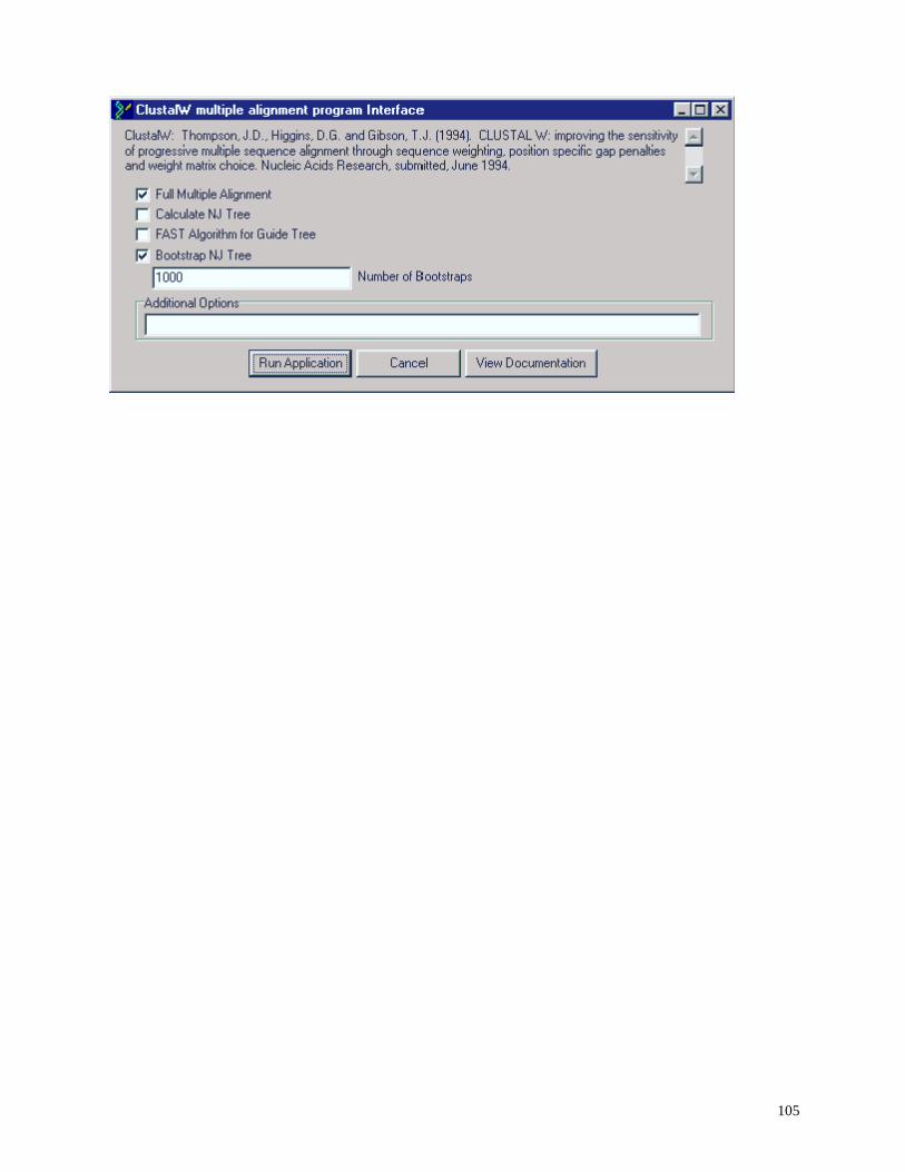
105
106
BLAST
A BLAST (Basic Local Alignment Search Tool) search is often the most convenient method
for detecting homology of a biological sequence to existing characterized sequences. BLAST
looks for homology by searching for locally aligned regions of identity and/or similarity between
a query sequence and sequences in a database. The algorithm works by the following general
method:
1. A query sequence is divided into short sequences (called words, ca. 3 to 8 residues, depending
on whether it’s protein or nucleic acid).
2. A table of all sequences of the same word size which can pair with each of the words from the
query sequence with a score above a defined threshold is constructed (the lookup table).
3. The database sequences are scanned for occurrence of sequences in the lookup table.
4. When a word is found in the database which can align to a word in the query over the critical
threshold, the alignment is extended in both directions. This extension continues in both
directions as long as the length of the extension does not exceed a defined limit without further
increasing the score of the alignment.
5. If, when an extension is terminated, the total sub-alignment score is above another defined
threshold, the alignment is reported.
6. When a threshold alignment is produced, that particular database sequence is re-scanned for
other non-redundant high-scoring segment pairs (HSPs) which score above yet another defined
cut-off (the sum of several non-significant sub-alignments within the same two sequences can,
when taken together, indicate significant similarity indicative of homology).
7. A statistical measure is reported which indicates the probability that a similar-scoring HSP or
set of HSPs found for a given query would result from searching the same database with a
randomly-generated sequence of the same length as the query.
For a reference on BLAST, see:
Altschul, Stephen F., Warren Gish, Webb Miller, Eugene W. Myers, and David J. Lipman
(1990). Basic local alignment search tool. J. Mol. Biol. 215:403-10.
and, for the newer gapped BLAST and PSI-BLAST versions,
Altschul, Stephen F., Thomas L. Madden, Alejandro A. Schäffer, Jinghui Zhang, Zheng Zhang,
Webb Miller, and David J. Lipman (1997), "Gapped BLAST and PSI-BLAST: a new generation
of protein database search programs", Nucleic Acids Res. 25:3389-3402.
for a description of the newer PHI-BLAST method, see:
Zhang, Zheng, Alejandro A. Schäffer, Webb Miller, Thomas L. Madden, David J. Lipman,
Eugene V. Koonin and Stephen F. Altschul (1998), "Protein sequence similarity searches using
patterns as seeds", Nucleic Acids Res. 26:3986-3990.
107
BLAST Programs
BLAST offers the following programs:
blastn: Search a nucleotide database with a nucleotide query
blastp: Search protein database with a protein query
tblastn: Search a six-frame dynamic translation of a nucleotide database with a protein query
blastx: Search a protein database with a six-frame translation of a nucleotide query sequence.
tblastx: Search a six-frame translation of a nucleotide database with a six-frame translation of a
nucleotide query sequence (very slow).
Local BLAST
The NCBI BLAST version 2.0.3 ( [Nov-14-1997], Altschul, Stephen F., Thomas L. Madden,
Alejandro A. Schaffer, Jinghui Zhang, Zheng Zhang, Webb Miller, and David J. Lipman (1997),
"Gapped BLAST and PSI-BLAST: a new generation of protein database search programs",
Nucleic Acids Res. 25:3389-3402.) is included in the BioEdit distribution and is found in the
\apps folder of the install directory. This is particular useful if you are interested in fishing out a
specific gene from a partially sequenced genome whose sequences have not yet been assigned
and deposited.
To use this program, you must first create a local database. You can create as many local
databases as you want, just keep in mind the following requirements:
1. Nucleotide and protein databases are separate entities.
2. Databases must be present within the \database directory of the BioEdit folder to be
recognized by the BioEdit local BLAST interface (the NCBI blastall.exe program, however, is a
stand-alone app that can be used entirely separately from BioEdit). When a database is created
using BioEdit, it is automatically placed into the \database directory.
Creating a local database
To create a local protein or nucleotide database for BLAST searching, you need only have a
Fasta-format file containing all of the sequences you want in the database. Nucleotide and
protein sequences cannot be mixed within the same database. From the “Accessory Application”
menu, choose “BLAST”, then “Create a local ... database file”. You will be prompted for the
input Fasta file. The rest is automatic. The database will be placed in to the \database folder of
the BioEdit install directory. The new database should appear in the appropriate database list
box of the local BLAST interface form.
Note: If you create a database or copy one into the \database folder, and it does not appear in the
choices on the BLAST search form, try quitting BioEdit and restarting. If this does not work,
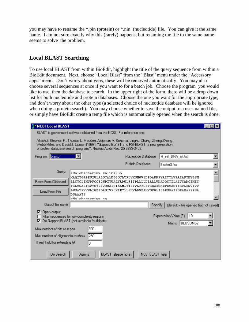
108
you may have to rename the *.pin (protein) or *.nin (nucleotide) file. You can give it the same
name. I am not sure exactly why this (rarely) happens, but renaming the file to the same name
seems to solve the problem.
Local BLAST Searching
To use local BLAST from within BioEdit, highlight the title of the query sequence from within a
BioEdit document. Next, choose “Local Blast” from the “Blast” menu under the “Accessory
apps” menu. Don’t worry about gaps, these will be removed automatically. You may also
choose several sequences at once if you want to for a batch job. Choose the program you would
like to use, then the database to search. In the upper right of the form, there will be a drop-down
list for both nucleotide and protein databases. Choose the one you want for the appropriate type,
and don’t worry about the other type (a selected choice of nucleotide database will be ignored
when doing a protein search). You may choose whether to save the output to a user-named file,
or simply have BioEdit create a temp file which is automatically opened when the search is done.
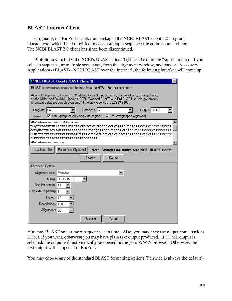
109
BLAST Internet Client
Originally, the BioEdit installation packaged the NCBI BLAST client 2.0 program
blatstcli.exe, which I had modified to accept an input sequence file at the command line.
The NCBI BLAST 2.0 client has since been discontinued.
BioEdit now includes the NCBI's BLAST client 3 (blastcl3.exe in the "/apps" folder). If you
select a sequence, or multiple sequences, from the alignment window, and choose "Accessory
Applications->BLAST->NCBI BLAST over the Internet", the following interface will come up:
You may BLAST one or more sequences at a time. Also, you may have the output come back as
HTML if you want, otherwise you may have plain text output produced. If HTML output is
selected, the output will automatically be opened in the your WWW browser. Otherwise, the
text output will be opened in BioEdit.
You may choose any of the standard BLAST formatting options (Pairwise is always the default):
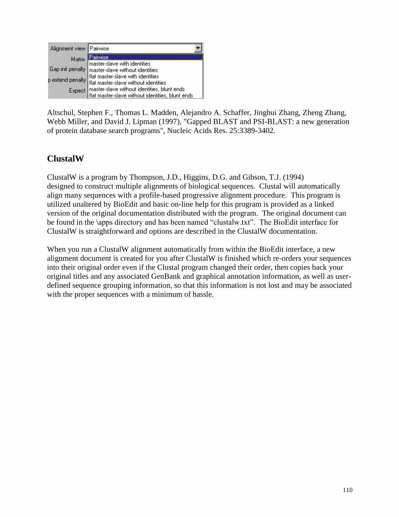
110
Altschul, Stephen F., Thomas L. Madden, Alejandro A. Schaffer, Jinghui Zhang, Zheng Zhang,
Webb Miller, and David J. Lipman (1997), "Gapped BLAST and PSI-BLAST: a new generation
of protein database search programs", Nucleic Acids Res. 25:3389-3402.
ClustalW
ClustalW is a program by Thompson, J.D., Higgins, D.G. and Gibson, T.J. (1994)
designed to construct multiple alignments of biological sequences. Clustal will automatically
align many sequences with a profile-based progressive alignment procedure. This program is
utilized unaltered by BioEdit and basic on-line help for this program is provided as a linked
version of the original documentation distributed with the program. The original document can
be found in the \apps directory and has been named “clustalw.txt”. The BioEdit interface for
ClustalW is straightforward and options are described in the ClustalW documentation.
When you run a ClustalW alignment automatically from within the BioEdit interface, a new
alignment document is created for you after ClustalW is finished which re-orders your sequences
into their original order even if the Clustal program changed their order, then copies back your
original titles and any associated GenBank and graphical annotation information, as well as user-
defined sequence grouping information, so that this information is not lost and may be associated
with the proper sequences with a minimum of hassle.
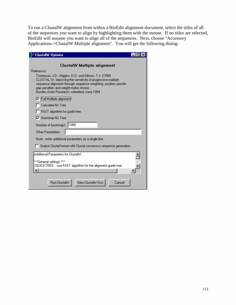
111
To run a ClustalW alignment from within a BioEdit alignment document, select the titles of all
of the sequences you want to align by highlighting them with the mouse. If no titles are selected,
BioEdit will assume you want to align all of the sequences. Next, choose "Accessory
Applications->ClustalW Multiple alignment". You will get the following dialog:
112
Using World Wide Web tools
Automated links
Restriction Mapping with Webcutter
If you have access to the World Wide Web, there is an automatic link to WebCutter, a web tool
for generating restriction maps. Simply highlight your sequence title in the edit window and
Choose “Auto-fed Restriction Mapping” from the “World Wide Web” menu. There are some
options to choose from, then press the “Analyze Sequence” button. In a short time your map will
be returned and reformatted. You may also use this feature with your external browser (which
may be necessary to fully view large maps).
BioEdit now also has an internal restriction map utility which has several nice options.
HTML BLAST with a Web Browser
This is general BLAST at NCBI. The only difference between using this feature and using
Netscape or Internet Explorer is that a selected sequence is automatically degapped and entered
into the query window of the BLAST form. If this feature is used with an external browser from
within BioEdit, however, the sequence is degapped and fed directly to the form. The most
obvious benefit of World Wide Web BLAST over the BLAST client program is that the resulting
hits have easy links directly to ENTREZ entries and to Medline abstracts. Since the BLAST
client program is just over 1 megabyte on disk, I may not include it in the next version of BioEdit
to make a smaller installation.
To use WWW BLAST from a BioEdit document, select the sequence title of interest and choose
“Auto-fed NCBI Standard BLAST” from the “World Wide Web” menu.
PSI-BLAST
PSI-BLAST is the newest search algorithm offered by NCBI. It is a variation on the original
BLAST algorithm and is embellished to provide a search method analogous to searching with a
consensus matrix defined by a set of homologous sequences in order to get a more sensitive
measure of distant homology.
PSI-BLAST (Position-Specific Iterated BLAST) is an extension to standard BLAST which
creates a position-specific weighted consensus matrix based upon an alignment of all high
scoring segment pairs (HSPs) scoring above a defined threshold resulting from a standard
BLAST search with the original query. During iterations of PSI-BLAST, the matrix is used in
place of the original query. The matrix is refined at each iteration. In most cases, the matrix
eventually converges to a point at which further iterations do not change the matrix. The
resulting position-weighted alignments may give a strong indication of distant homologies that
would be entirely missed with a single standard BLAST search.
113
For further reading on PSI-BLAST, see:
Altschul, Stephen F., Thomas L. Madden, Alejandro A. Schäffer, Jinghui Zhang, Zheng Zhang,
Webb Miller, and David J. Lipman (1997), "Gapped BLAST and PSI-BLAST: a new generation
of protein database search programs", Nucleic Acids Res. 25:3389-3402.
PHI-BLAST
PHI-BLAST (Pattern-Hit Initiated BLAST) searches for a user-specified pattern, or motif, and
reports on BLAST-like local alignments that are seeded around the pattern-matched region.
For more information on PHI-BLAST see:
http://www2.ncbi.nlm.nih.gov/BLAST/phiblast.html
For the paper describing PHI-BLAST, see:
Zhang, Zheng, Alejandro A. Schäffer, Webb Miller, Thomas L. Madden, David J. Lipman,
Eugene V. Koonin, and Stephen F. Altschul (1998), "Protein sequence similarity searches using
patterns as seeds", Nucleic Acids Res.26:3986-3990.
Prosite profile and pattern scans
Automated links to web pages (saved locally in the apps folder) are provided for Prosite profile
and pattern scans. For more information about Prosite, see:
http://www.expasy.ch/prosite/
A profilescan compares a protein or nucleic acid sequence against a profile library.
A pattern scan scans a protein sequence for the occurrence of patterns stored in the Prosite
database.
Both of these options may be found under Sequence->World Wide Web.
For a paper describing the Prosite database, see:
Hofmann, K., Bucher, P., Falquet, L., and Bairoch, A. (1999) The PROSITE database, its status
in 1999. Nucleic Acids Res. 27:215-219.
nnPredict protein secondary structure prediction
114
Please note: The following brief information is taken directly from
http://www.cmpharm.ucsf.edu/~nomi/nnpredict-instrucs.html
I am not qualified to discuss neural networks and parallel processing and BioEdit does not
perform any protein structure prediction, but simply provides a link to this program through the
World Wide Web.
"nnpredict is a program which uses a neural-network approach for predicting the secondary
structure type for each residue in an amino acid sequence. nnpredict was written by Donald
Kneller (Copyright (C) 1991 Regents of the University of California), and a WWW interface (the
interface linked to by BioEdit) was written by Nomi Harris ([email protected],
For papers describing the algorithm and distributed processing methodology, see:
D. G. Kneller, F. E. Cohen and R. Langridge (1990) "Improvements in Protein Secondary
Structure Prediction by an Enhanced Neural Network" J. Mol. Biol. (214) 171-182.
J. L. McClelland and D. E. Rumelhart. (1988) "Explorations in Parallel Distributed Processing"
vol 3. pp 318-362. MIT Press, Cambridge MA.
Other links
Entrez and PubMed
These sites are maintained by the NCBI (National Center for Biotechnology Information:
http://www.ncbi.nlm.nih.gov). PubMed contains the full Medline indexes freely available to the
public.
Pedro’s BioMolecular Research Tools
This site contains a plethora of biotechnology and molecular biology links, especially to services
available through server programs over the World Wide Web.
115
Constructing World Wide Web Bookmarks for BioEdit
BioEdit may store up to 500 World Wide Web bookmarks for which appear in the World Wide
Web menu at startup. These bookmarks may be used with your favorite external Web browser
as a convenient link to sequence analysis-related web sites from within a sequence editor.
The BioEdit web bookmarks are stored in a raw text file called “bookmark.txt”. This file is
found in the “apps” folder of the install directory. If the name of this file is changed, BioEdit
will not recognize it. If this file is corrupted, BioEdit will allow you to automatically write a
default file with some canned bookmarks.
The required format for the bookmarks file is very simple. Each entry consists of two lines of
text, one for the description and one for the URL. The format is as follows:
name=<description>
address=<exact URL>
The following example shows the default bookmarks file that comes with BioEdit (or did at one
time):
name=WebCutter Restriction Map Generator
address=http://www.firstmarket.com/cutter/cut2.html
name=BLAST at NCBI
address=http://www.ncbi.nlm.nih.gov/cgi-bin/BLAST/nph-blast?Jform=1
name=PSI-BLAST at NCBI
address=http://www.ncbi.nlm.nih.gov/cgi-bin/BLAST/nph-psi_blast
name=Pub Med Literature Search
address=http://www.ncbi.nlm.nih.gov/PubMed/medline.html
name=National Center for Biotechnology information
address=http://www.ncbi.nlm.nih.gov/
name=Pedro's BioMolecular Research Tools
address=http://www.fmi.ch/biology/research_tools.html
name=information about sequence logos (Tom Schneider)
address=http://www.bio.cam.ac.uk/seqlogo/
name=Sequence logo submission form
address=http://www.bio.cam.ac.uk/cgi-bin/seqlogo/logo.cgi
name=The Institute for Genomic Research (TIGR)
address=http://www.tigr.org/tigr_home/index.html
name=The RNase P Database
address=http://www.mbio.ncsu.edu/RNaseP/home.html
name=NCSU Microbiology Web Server
address=http://www.mbio.ncsu.edu/
That’s all there is to it. If a bookmark entry is not formatted correctly, it will be ignored.
If you have made an entry and it does not appear in the World Wide Web menu after restarting
BioEdit, check the entry to make sure the format matches exactly.

116
You may edit the bookmarks in any text editor. You may also edit them by choosing “View
bookmarks” from the World Wide Web menu. The bookmarks will appear in a text window
with the option to edit and save. At this time there is no graphical interface for bookmark
manipulation.
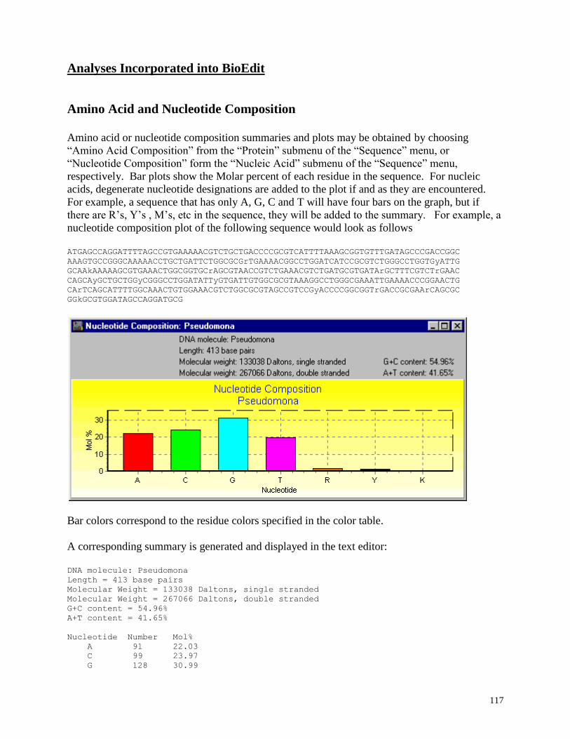
117
Analyses Incorporated into BioEdit
Amino Acid and Nucleotide Composition
Amino acid or nucleotide composition summaries and plots may be obtained by choosing
“Amino Acid Composition” from the “Protein” submenu of the “Sequence” menu, or
“Nucleotide Composition” form the “Nucleic Acid” submenu of the “Sequence” menu,
respectively. Bar plots show the Molar percent of each residue in the sequence. For nucleic
acids, degenerate nucleotide designations are added to the plot if and as they are encountered.
For example, a sequence that has only A, G, C and T will have four bars on the graph, but if
there are R’s, Y’s , M’s, etc in the sequence, they will be added to the summary. For example, a
nucleotide composition plot of the following sequence would look as follows
ATGAGCCAGGATTTTAGCCGTGAAAAACGTCTGCTGACCCCGCGTCATTTTAAAGCGGTGTTTGATAGCCCGACCGGC
AAAGTGCCGGGCAAAAACCTGCTGATTCTGGCGCGrTGAAAACGGCCTGGATCATCCGCGTCTGGGCCTGGTGyATTG
GCAAkAAAAAGCGTGAAACTGGCGGTGCrAGCGTAACCGTCTGAAACGTCTGATGCGTGATArGCTTTCGTCTrGAAC
CAGCAyGCTGCTGGyCGGGCCTGGATATTyGTGATTGTGGCGCGTAAAGGCCTGGGCGAAATTGAAAACCCGGAACTG
CArTCAGCATTTTGGCAAACTGTGGAAACGTCTGGCGCGTAGCCGTCCGyACCCCGGCGGTrGACCGCGAArCAGCGC
GGkGCGTGGATAGCCAGGATGCG
Bar colors correspond to the residue colors specified in the color table.
A corresponding summary is generated and displayed in the text editor:
DNA molecule: Pseudomona
Length = 413 base pairs
Molecular Weight = 133038 Daltons, single stranded
Molecular Weight = 267066 Daltons, double stranded
G+C content = 54.96%
A+T content = 41.65%
Nucleotide Number Mol%
A 91 22.03
C 99 23.97
G 128 30.99
118
T 81 19.61
R 7 1.69
Y 5 1.21
K 2 0.48
Amino Acid plots and summaries are similar, though residues other than the standard 20 amino
acids are ignored.
Molecular weights:
The molecular weights of proteins are calculated as the sum of the internal molecular weights of
each amino acid, or
where R = the side group, plus 2 hydrogens and an oxygen at the amino and
carboxy termini, respectively.
Nucleotide weights are calculated as the sum of the monophosphate forms of each ribonucleotide
or deoxyribonucleotide minus one water each. One water (18 Da) is added at the end to
represent the 3’ hydroxyl at the end of the chain and one more hydrogen at the 5’ phosphate end.
Nucleotide weights used are:
RNA M.W.
Adenosine 328.2
Guanosine 344.2
Cytidine 304.2
Uridine 305.2
Average AUGC 320.5
DNA
dAdenosine 312.2
dGuanosine 328.2
dCytidine 288.2
dThymidine 287.2
Average dATGC 304.0
These values were derived by adding all atoms in each nucleotide monophosphate minus one
oxygen and two hydrogens using:
C = 12.011
O = 15.9994
N = 14.00674
P = 30.973762
H = 1.00794
119
Entropy plots
An entropy plot can give an idea of the amount of variability through a column in an
alignment. It is a measure of the lack of “information content” at each position in the alignment.
More accurately, it is a measure of the lack of predictability for an alignment position. If there
are x sequences in an alignment (say x = 40 sequences) of DNA sequences, and at position y (say
y = position 5) there is an ‘A’ in all sequences, we can assume we have a lot of information for
position 5 and chances are if we had to guess at the base at position 5 of another homologous
sequence, we would be correct to guess ‘A’. We have maximum “information” for position 5,
and the entropy is 0. Now, if there are four possibilities for each position (A, G, C or T) and
each occurs at position 5 with a frequency of 0.25 (equally probable), then our information
content (how well we could predict the position for a new incoming sequence) has been reduced
to 0, and the entropy is at maximum variability.
Information is often measured in bits, which are basically either/or (yes/no, on/off) units, or a
base-2 number system. If there are 4 possible residues at a given position, then two bits of
information are required to determine the base at that position (e.g.., purine or pyrimidine? = 1
bit, if purine, ‘A’ or ‘G’? = 1 more bit -- 2 bits total). For proteins (with 20 amino acids) at most
5 bits are required (e.g.. 1st 10? -- 1 bit, 1
st 5 of block of 10? -- 1 more bit, 1
st 3 of block of 5?, 1
st
2 of 3?, 1st 1 or 2?: = 5 yes/no answers). If a position in an alignment can take any of four
positions, but always turns up ‘A’, we have no uncertainty at that position and therefore can say
we have maximum (two bits) of information.
Mathematically, the basis of information theory was defined by Claude Shannon:
H(l) = -f(b,l)log(base 2)f(b,l) (measured in bits)
where H(l) = the uncertainty, also called entropy at position l, b represents a residue (out of the
allowed choices for the sequence in question), and f(b,l) is the frequency at which residue b is
found at position l. The information content of a position l, then, is defined as a decrease in
uncertainty or entropy at that position. As an alignment improves in quality, therefore, the
entropy at each position (especially conserved regions) should decrease.
BioEdit plots the entropy at each position, rather than the information content, because, in order
to determine information at a position, the total number of possible residues must be known.
This will vary depending on whether one wishes to include gaps or degenerate nucleotide bases
such as S, M, K, W, etc. in the analysis. For entropy plotting, the sequences are treated as a
matrix of characters. Entropy at a column position is independent of the total information
possible at a given position, and depends only upon the frequencies of characters that appear in
that column. BioEdit uses the natural logarithm rather than log(base 2) for convenience, so the
values are actually in nits rather than bits, but the data are the same relative to each other.
Entropy is then calculated as H(l) = -f(b,l)ln(f(b,l)), which gives a measure of uncertainty at
each position relative to other positions. Maximum total uncertainty will be defined by the
maximum number of different characters found in a column. For example, if 20 amino acids and
gaps are represented, but no user-defined characters are present, then the maximum uncertainty
possible would be (21*(1/21)ln(1/21))=3.04 (if, say, there were 42 sequences in the alignment
and each character was represented exactly twice at a given column position). This measure is
not given in bits. Conversion to bits simply requires conversion to log base 2, however, and the
entropy calculation could be made as: H(l) = -f(b,l)*(ln(f(b,l)/ln2). This is not really necessary,
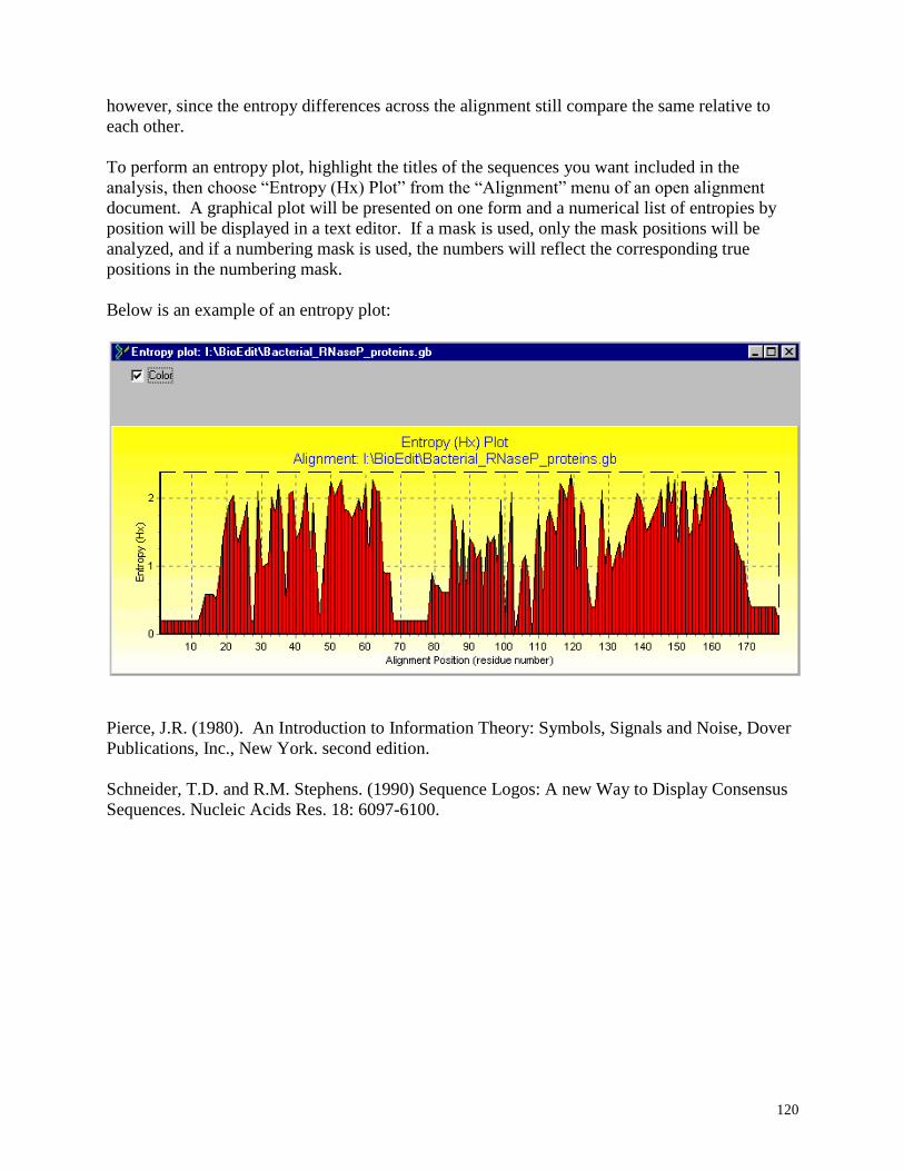
120
however, since the entropy differences across the alignment still compare the same relative to
each other.
To perform an entropy plot, highlight the titles of the sequences you want included in the
analysis, then choose “Entropy (Hx) Plot” from the “Alignment” menu of an open alignment
document. A graphical plot will be presented on one form and a numerical list of entropies by
position will be displayed in a text editor. If a mask is used, only the mask positions will be
analyzed, and if a numbering mask is used, the numbers will reflect the corresponding true
positions in the numbering mask.
Below is an example of an entropy plot:
Pierce, J.R. (1980). An Introduction to Information Theory: Symbols, Signals and Noise, Dover
Publications, Inc., New York. second edition.
Schneider, T.D. and R.M. Stephens. (1990) Sequence Logos: A new Way to Display Consensus
Sequences. Nucleic Acids Res. 18: 6097-6100.
121
Hydrophobicity Profiles
Mean Hydrophobicity profiles are generated using the general method of Kyte and Doolittle
(1982). Kyte and Doolittle compiled a set of “hydropathy scores” for the 20 amino acids based
upon a compilation of experimental data from the literature. A window of defined size is moved
along a sequence, the hydropathy scores are summed along the window, and the average (the
sum divided by the window size) is taken for each position in the sequence. The mean
hydrophobicity value is plotted for the middle residue of the window.
Hydrophobic moment profiles plot the hydrophobic moment of segments of defined length along
the sequence. For example, if the window size is 21 residues, the plotted value at a residue is the
hydrophobic moment of the window of ten residues on either side of the current residue.
Hydrophobic moment is calculated according to Eisenberg et. al. (1984):
= {[Hnsin(n)]^2 + [Hncos(n)]}^(1/2),
Where H is the hydrophobic moment, Hn is the hydrophobicity score of residue H at position n,
=100 degrees, n is position within the segment, and each hydrophobic moment is summed over
a segment of the same defined window length.
Mean hydrophobic moment profiles plot the average hydrophobic moment for a segment of
defined window length, using the same window width to calculate the hydrophobic moments.
For example, for a window size of 21, the hydrophobic moments of 21 segments, each 21
residues long and each value representing the start residue of the corresponding segment, are
summed and their average is taken and plotted for the center residue of the segment.
Previous versions of BioEdit simply plotted the mean hydrophobicity of a sequence segment at
the first position of the segment. The result was that the mean hydrophobicity at the end of the
plot, after the point L-W, where L is the sequence length and W is the window size, the mean
value would become deceptively closer to 0. The current method is more akin to the method of
Kyte and Doolittle, and may be more familiar.
Note: I do not have the expertise to make any claims about the predictive power of these profile
plots. BioEdit makes no conclusions about hydrophobic and/or transmembrane segments of
proteins, and interpretation of these plots is up to the judgment of the user.
For information and references about hydrophobicity analysis of proteins, see:
Cornette, J.L., K.B. Cease, H. Margalit, J.L. Spouge, J.A. Berzofsky and C. DeList. 1987.
Hydrophobicity Scales and Computational Techniques for Detecting Amphipathic Structures in
Proteins. J. Mol. Biol. 195: 659-685.
Eisenberg D. E. Schwarz, M. Komaromy and R.Wall. 1984. Analysis of membrane and surface
protein sequences with the hydrophobic moment plot. J. Mol. Biol. 179(1):125-42.
Hopp, T.P. and K.R. Woods. 1981. Prediction of protein antigenic determinants from amino
acid sequences. Proc. Natl. Acad. Sci. USA. 78(6): 3824-3828.
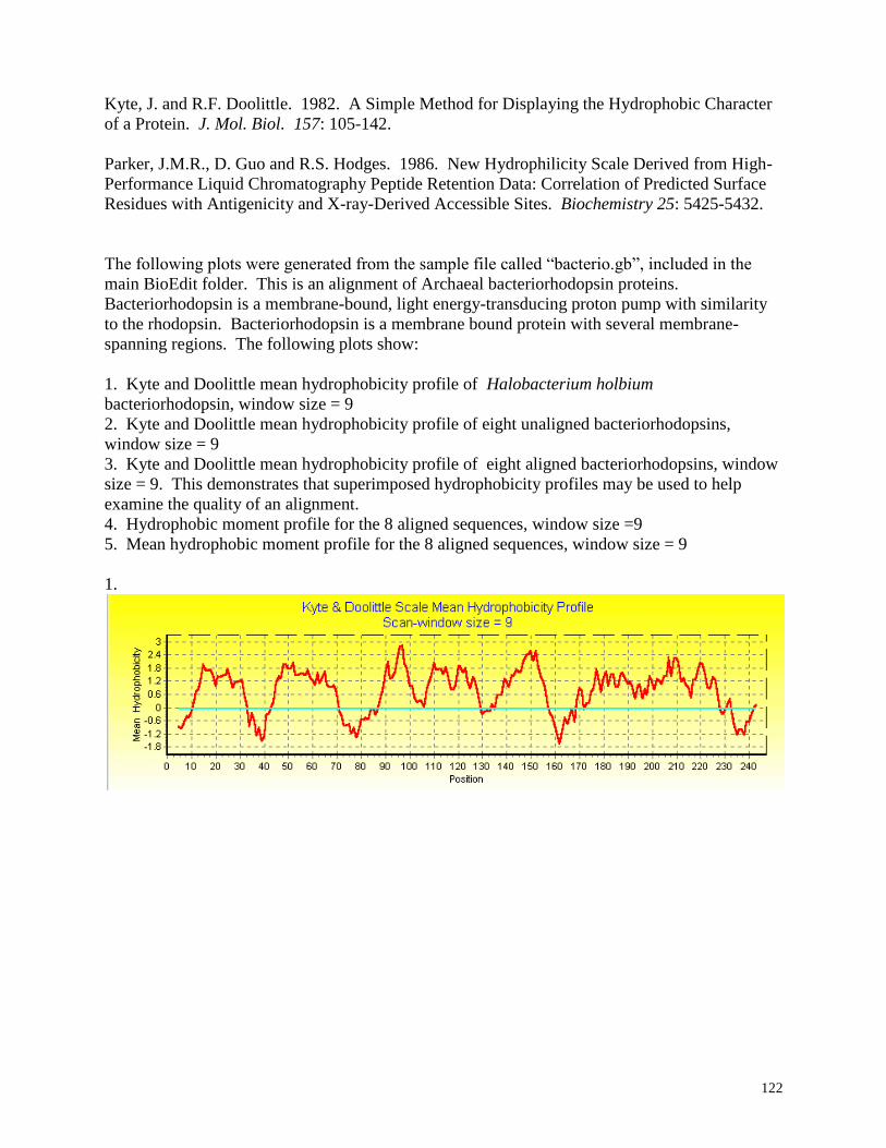
122
Kyte, J. and R.F. Doolittle. 1982. A Simple Method for Displaying the Hydrophobic Character
of a Protein. J. Mol. Biol. 157: 105-142.
Parker, J.M.R., D. Guo and R.S. Hodges. 1986. New Hydrophilicity Scale Derived from High-
Performance Liquid Chromatography Peptide Retention Data: Correlation of Predicted Surface
Residues with Antigenicity and X-ray-Derived Accessible Sites. Biochemistry 25: 5425-5432.
The following plots were generated from the sample file called “bacterio.gb”, included in the
main BioEdit folder. This is an alignment of Archaeal bacteriorhodopsin proteins.
Bacteriorhodopsin is a membrane-bound, light energy-transducing proton pump with similarity
to the rhodopsin. Bacteriorhodopsin is a membrane bound protein with several membrane-
spanning regions. The following plots show:
1. Kyte and Doolittle mean hydrophobicity profile of Halobacterium holbium
bacteriorhodopsin, window size = 9
2. Kyte and Doolittle mean hydrophobicity profile of eight unaligned bacteriorhodopsins,
window size = 9
3. Kyte and Doolittle mean hydrophobicity profile of eight aligned bacteriorhodopsins, window
size = 9. This demonstrates that superimposed hydrophobicity profiles may be used to help
examine the quality of an alignment.
4. Hydrophobic moment profile for the 8 aligned sequences, window size =9
5. Mean hydrophobic moment profile for the 8 aligned sequences, window size = 9
1.
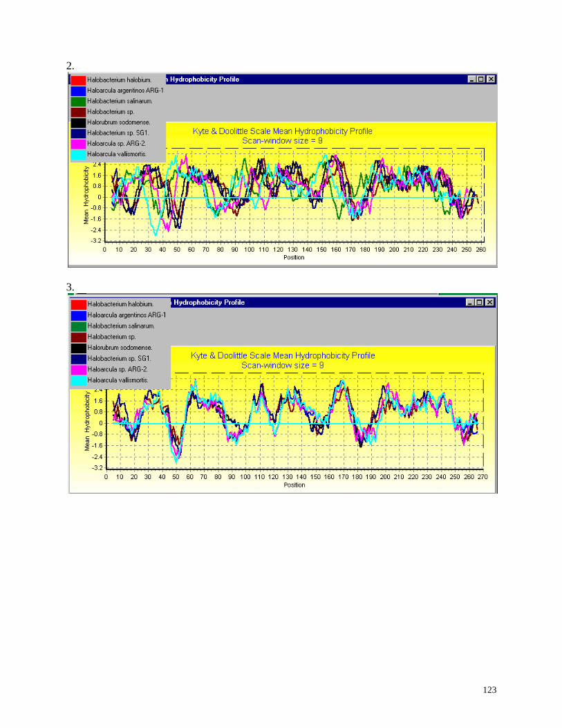
123
2.
3.
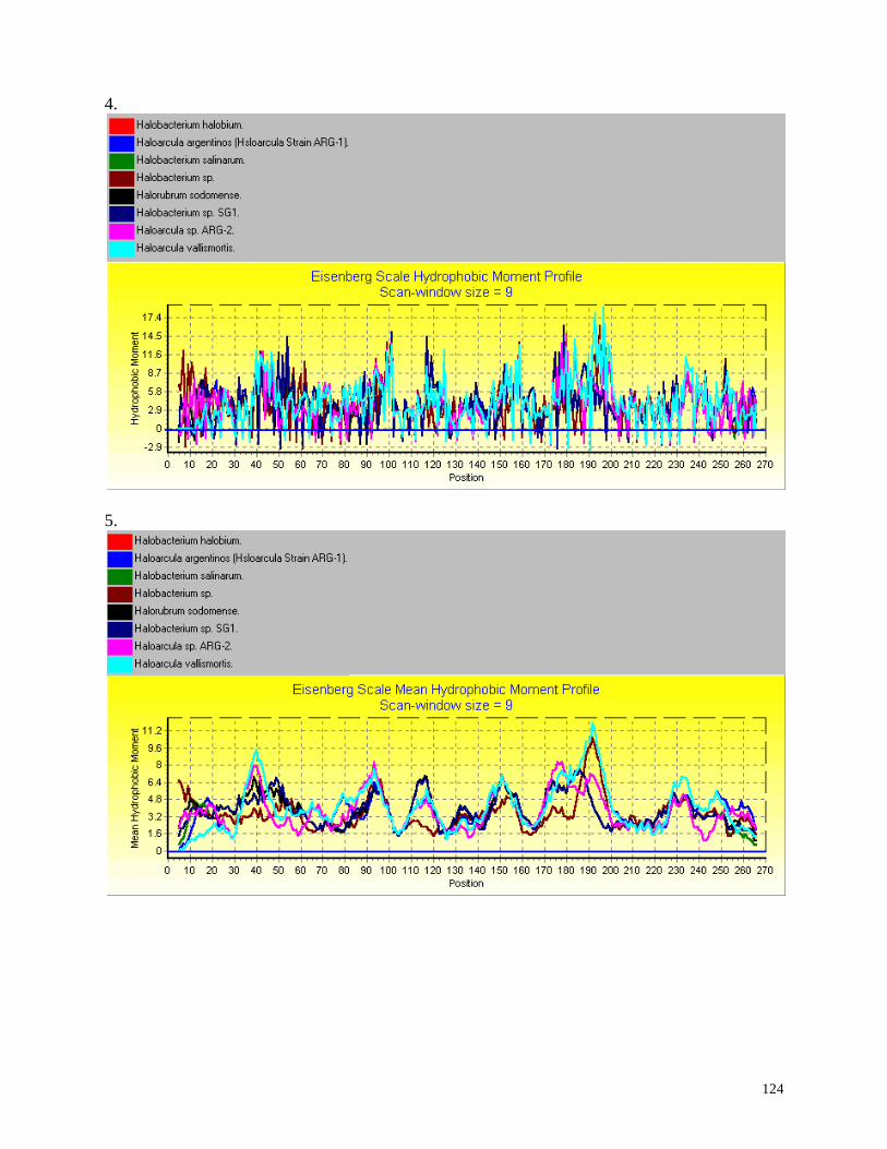
124
4.
5.
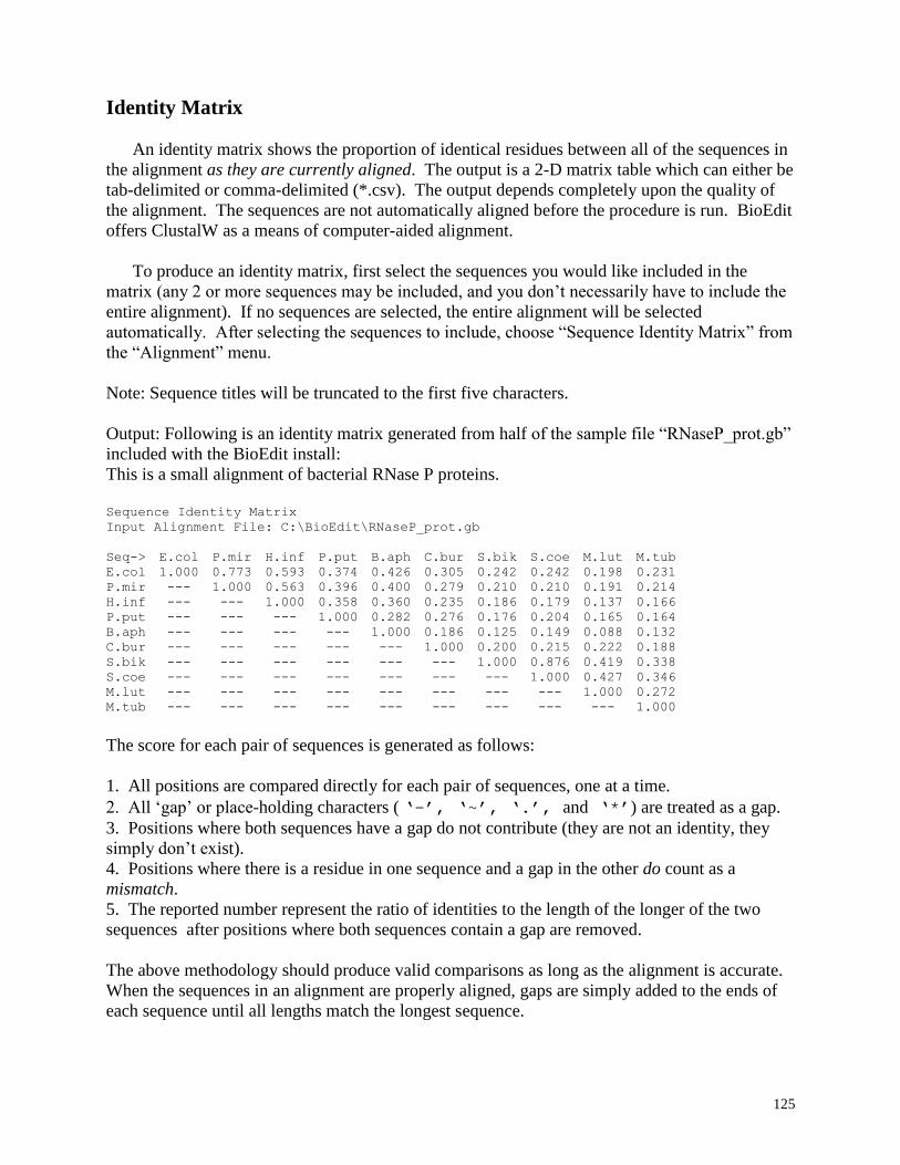
125
Identity Matrix
An identity matrix shows the proportion of identical residues between all of the sequences in
the alignment as they are currently aligned. The output is a 2-D matrix table which can either be
tab-delimited or comma-delimited (*.csv). The output depends completely upon the quality of
the alignment. The sequences are not automatically aligned before the procedure is run. BioEdit
offers ClustalW as a means of computer-aided alignment.
To produce an identity matrix, first select the sequences you would like included in the
matrix (any 2 or more sequences may be included, and you don’t necessarily have to include the
entire alignment). If no sequences are selected, the entire alignment will be selected
automatically. After selecting the sequences to include, choose “Sequence Identity Matrix” from
the “Alignment” menu.
Note: Sequence titles will be truncated to the first five characters.
Output: Following is an identity matrix generated from half of the sample file “RNaseP_prot.gb”
included with the BioEdit install:
This is a small alignment of bacterial RNase P proteins.
Sequence Identity Matrix
Input Alignment File: C:\BioEdit\RNaseP_prot.gb
Seq-> E.col P.mir H.inf P.put B.aph C.bur S.bik S.coe M.lut M.tub
E.col 1.000 0.773 0.593 0.374 0.426 0.305 0.242 0.242 0.198 0.231
P.mir --- 1.000 0.563 0.396 0.400 0.279 0.210 0.210 0.191 0.214
H.inf --- --- 1.000 0.358 0.360 0.235 0.186 0.179 0.137 0.166
P.put --- --- --- 1.000 0.282 0.276 0.176 0.204 0.165 0.164
B.aph --- --- --- --- 1.000 0.186 0.125 0.149 0.088 0.132
C.bur --- --- --- --- --- 1.000 0.200 0.215 0.222 0.188
S.bik --- --- --- --- --- --- 1.000 0.876 0.419 0.338
S.coe --- --- --- --- --- --- --- 1.000 0.427 0.346
M.lut --- --- --- --- --- --- --- --- 1.000 0.272
M.tub --- --- --- --- --- --- --- --- --- 1.000
The score for each pair of sequences is generated as follows:
1. All positions are compared directly for each pair of sequences, one at a time.
2. All ‘gap’ or place-holding characters ( ‘-’, ‘~’, ‘.’, and ‘*’) are treated as a gap.
3. Positions where both sequences have a gap do not contribute (they are not an identity, they
simply don’t exist).
4. Positions where there is a residue in one sequence and a gap in the other do count as a
mismatch.
5. The reported number represent the ratio of identities to the length of the longer of the two
sequences after positions where both sequences contain a gap are removed.
The above methodology should produce valid comparisons as long as the alignment is accurate.
When the sequences in an alignment are properly aligned, gaps are simply added to the ends of
each sequence until all lengths match the longest sequence.
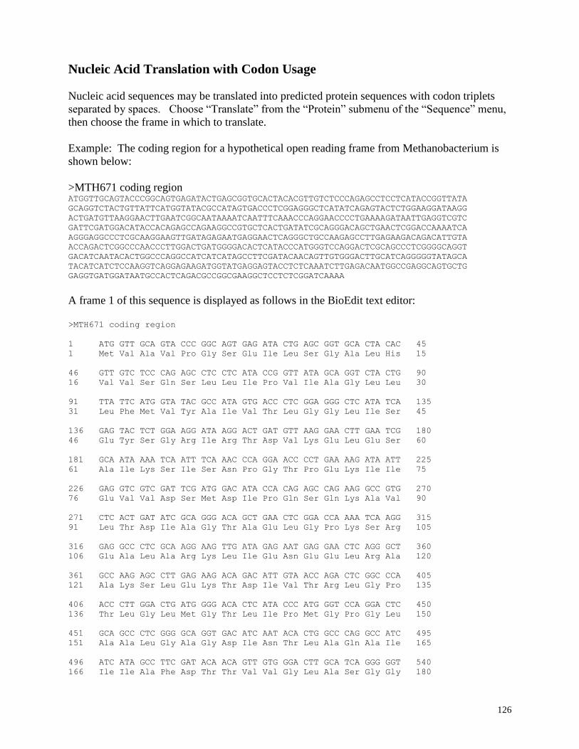
126
Nucleic Acid Translation with Codon Usage
Nucleic acid sequences may be translated into predicted protein sequences with codon triplets
separated by spaces. Choose “Translate” from the “Protein” submenu of the “Sequence” menu,
then choose the frame in which to translate.
Example: The coding region for a hypothetical open reading frame from Methanobacterium is
shown below:
>MTH671 coding region ATGGTTGCAGTACCCGGCAGTGAGATACTGAGCGGTGCACTACACGTTGTCTCCCAGAGCCTCCTCATACCGGTTATA
GCAGGTCTACTGTTATTCATGGTATACGCCATAGTGACCCTCGGAGGGCTCATATCAGAGTACTCTGGAAGGATAAGG
ACTGATGTTAAGGAACTTGAATCGGCAATAAAATCAATTTCAAACCCAGGAACCCCTGAAAAGATAATTGAGGTCGTC
GATTCGATGGACATACCACAGAGCCAGAAGGCCGTGCTCACTGATATCGCAGGGACAGCTGAACTCGGACCAAAATCA
AGGGAGGCCCTCGCAAGGAAGTTGATAGAGAATGAGGAACTCAGGGCTGCCAAGAGCCTTGAGAAGACAGACATTGTA
ACCAGACTCGGCCCAACCCTTGGACTGATGGGGACACTCATACCCATGGGTCCAGGACTCGCAGCCCTCGGGGCAGGT
GACATCAATACACTGGCCCAGGCCATCATCATAGCCTTCGATACAACAGTTGTGGGACTTGCATCAGGGGGTATAGCA
TACATCATCTCCAAGGTCAGGAGAAGATGGTATGAGGAGTACCTCTCAAATCTTGAGACAATGGCCGAGGCAGTGCTG
GAGGTGATGGATAATGCCACTCAGACGCCGGCGAAGGCTCCTCTCGGATCAAAA
A frame 1 of this sequence is displayed as follows in the BioEdit text editor:
>MTH671 coding region
1 ATG GTT GCA GTA CCC GGC AGT GAG ATA CTG AGC GGT GCA CTA CAC 45
1 Met Val Ala Val Pro Gly Ser Glu Ile Leu Ser Gly Ala Leu His 15
46 GTT GTC TCC CAG AGC CTC CTC ATA CCG GTT ATA GCA GGT CTA CTG 90
16 Val Val Ser Gln Ser Leu Leu Ile Pro Val Ile Ala Gly Leu Leu 30
91 TTA TTC ATG GTA TAC GCC ATA GTG ACC CTC GGA GGG CTC ATA TCA 135
31 Leu Phe Met Val Tyr Ala Ile Val Thr Leu Gly Gly Leu Ile Ser 45
136 GAG TAC TCT GGA AGG ATA AGG ACT GAT GTT AAG GAA CTT GAA TCG 180
46 Glu Tyr Ser Gly Arg Ile Arg Thr Asp Val Lys Glu Leu Glu Ser 60
181 GCA ATA AAA TCA ATT TCA AAC CCA GGA ACC CCT GAA AAG ATA ATT 225
61 Ala Ile Lys Ser Ile Ser Asn Pro Gly Thr Pro Glu Lys Ile Ile 75
226 GAG GTC GTC GAT TCG ATG GAC ATA CCA CAG AGC CAG AAG GCC GTG 270
76 Glu Val Val Asp Ser Met Asp Ile Pro Gln Ser Gln Lys Ala Val 90
271 CTC ACT GAT ATC GCA GGG ACA GCT GAA CTC GGA CCA AAA TCA AGG 315
91 Leu Thr Asp Ile Ala Gly Thr Ala Glu Leu Gly Pro Lys Ser Arg 105
316 GAG GCC CTC GCA AGG AAG TTG ATA GAG AAT GAG GAA CTC AGG GCT 360
106 Glu Ala Leu Ala Arg Lys Leu Ile Glu Asn Glu Glu Leu Arg Ala 120
361 GCC AAG AGC CTT GAG AAG ACA GAC ATT GTA ACC AGA CTC GGC CCA 405
121 Ala Lys Ser Leu Glu Lys Thr Asp Ile Val Thr Arg Leu Gly Pro 135
406 ACC CTT GGA CTG ATG GGG ACA CTC ATA CCC ATG GGT CCA GGA CTC 450
136 Thr Leu Gly Leu Met Gly Thr Leu Ile Pro Met Gly Pro Gly Leu 150
451 GCA GCC CTC GGG GCA GGT GAC ATC AAT ACA CTG GCC CAG GCC ATC 495
151 Ala Ala Leu Gly Ala Gly Asp Ile Asn Thr Leu Ala Gln Ala Ile 165
496 ATC ATA GCC TTC GAT ACA ACA GTT GTG GGA CTT GCA TCA GGG GGT 540
166 Ile Ile Ala Phe Asp Thr Thr Val Val Gly Leu Ala Ser Gly Gly 180
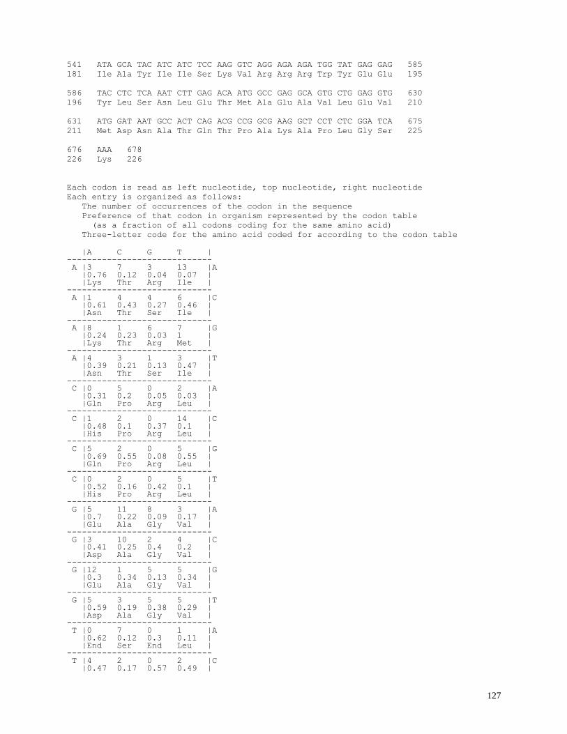
127
541 ATA GCA TAC ATC ATC TCC AAG GTC AGG AGA AGA TGG TAT GAG GAG 585
181 Ile Ala Tyr Ile Ile Ser Lys Val Arg Arg Arg Trp Tyr Glu Glu 195
586 TAC CTC TCA AAT CTT GAG ACA ATG GCC GAG GCA GTG CTG GAG GTG 630
196 Tyr Leu Ser Asn Leu Glu Thr Met Ala Glu Ala Val Leu Glu Val 210
631 ATG GAT AAT GCC ACT CAG ACG CCG GCG AAG GCT CCT CTC GGA TCA 675
211 Met Asp Asn Ala Thr Gln Thr Pro Ala Lys Ala Pro Leu Gly Ser 225
676 AAA 678
226 Lys 226
Each codon is read as left nucleotide, top nucleotide, right nucleotide
Each entry is organized as follows:
The number of occurrences of the codon in the sequence
Preference of that codon in organism represented by the codon table
(as a fraction of all codons coding for the same amino acid)
Three-letter code for the amino acid coded for according to the codon table
|A C G T | ----------------------------- A |3 7 3 13 |A |0.76 0.12 0.04 0.07 | |Lys Thr Arg Ile | ----------------------------- A |1 4 4 6 |C |0.61 0.43 0.27 0.46 | |Asn Thr Ser Ile | ----------------------------- A |8 1 6 7 |G |0.24 0.23 0.03 1 | |Lys Thr Arg Met | ----------------------------- A |4 3 1 3 |T |0.39 0.21 0.13 0.47 | |Asn Thr Ser Ile | ----------------------------- C |0 5 0 2 |A |0.31 0.2 0.05 0.03 | |Gln Pro Arg Leu | ----------------------------- C |1 2 0 14 |C |0.48 0.1 0.37 0.1 | |His Pro Arg Leu | ----------------------------- C |5 2 0 5 |G |0.69 0.55 0.08 0.55 | |Gln Pro Arg Leu | ----------------------------- C |0 2 0 5 |T |0.52 0.16 0.42 0.1 | |His Pro Arg Leu | ----------------------------- G |5 11 8 3 |A |0.7 0.22 0.09 0.17 | |Glu Ala Gly Val | ----------------------------- G |3 10 2 4 |C |0.41 0.25 0.4 0.2 | |Asp Ala Gly Val | ----------------------------- G |12 1 5 5 |G |0.3 0.34 0.13 0.34 | |Glu Ala Gly Val | ----------------------------- G |5 3 5 5 |T |0.59 0.19 0.38 0.29 | |Asp Ala Gly Val | ----------------------------- T |0 7 0 1 |A |0.62 0.12 0.3 0.11 | |End Ser End Leu | ----------------------------- T |4 2 0 2 |C |0.47 0.17 0.57 0.49 |
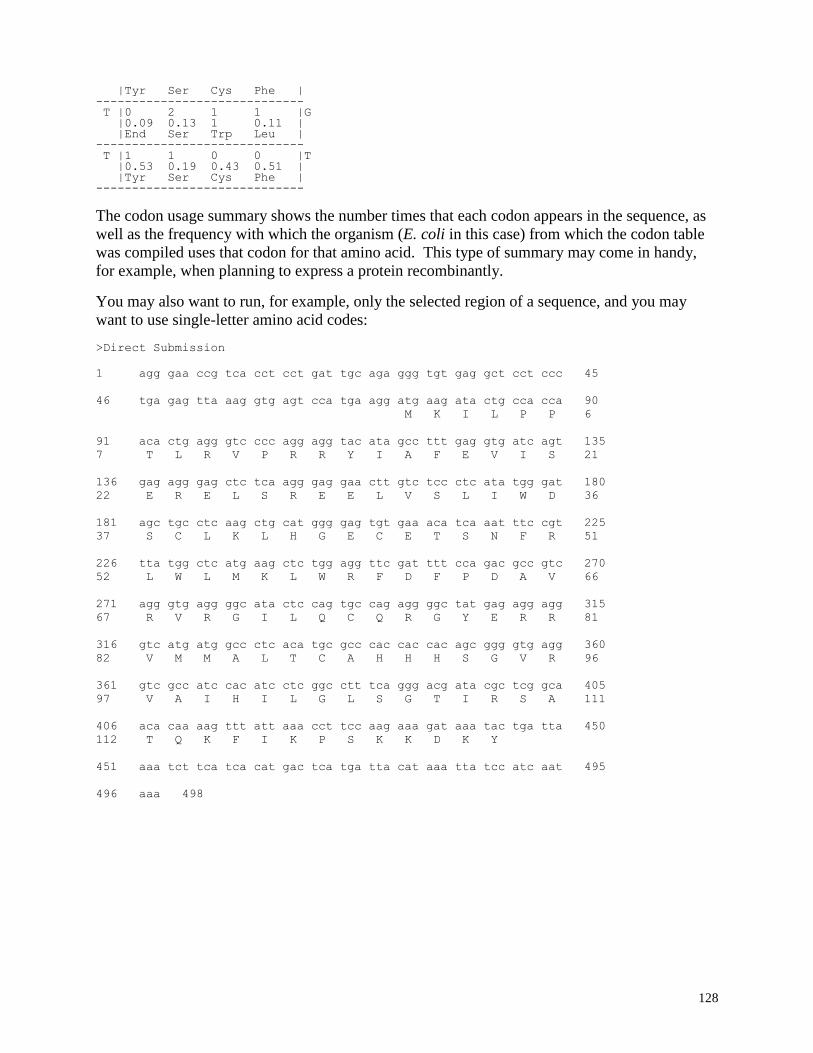
128
|Tyr Ser Cys Phe | ----------------------------- T |0 2 1 1 |G |0.09 0.13 1 0.11 | |End Ser Trp Leu | ----------------------------- T |1 1 0 0 |T |0.53 0.19 0.43 0.51 | |Tyr Ser Cys Phe | -----------------------------
The codon usage summary shows the number times that each codon appears in the sequence, as
well as the frequency with which the organism (E. coli in this case) from which the codon table
was compiled uses that codon for that amino acid. This type of summary may come in handy,
for example, when planning to express a protein recombinantly.
You may also want to run, for example, only the selected region of a sequence, and you may
want to use single-letter amino acid codes:
>Direct Submission
1 agg gaa ccg tca cct cct gat tgc aga ggg tgt gag gct cct ccc 45
46 tga gag tta aag gtg agt cca tga agg atg aag ata ctg cca cca 90
M K I L P P 6
91 aca ctg agg gtc ccc agg agg tac ata gcc ttt gag gtg atc agt 135
7 T L R V P R R Y I A F E V I S 21
136 gag agg gag ctc tca agg gag gaa ctt gtc tcc ctc ata tgg gat 180
22 E R E L S R E E L V S L I W D 36
181 agc tgc ctc aag ctg cat ggg gag tgt gaa aca tca aat ttc cgt 225
37 S C L K L H G E C E T S N F R 51
226 tta tgg ctc atg aag ctc tgg agg ttc gat ttt cca gac gcc gtc 270
52 L W L M K L W R F D F P D A V 66
271 agg gtg agg ggc ata ctc cag tgc cag agg ggc tat gag agg agg 315
67 R V R G I L Q C Q R G Y E R R 81
316 gtc atg atg gcc ctc aca tgc gcc cac cac cac agc ggg gtg agg 360
82 V M M A L T C A H H H S G V R 96
361 gtc gcc atc cac atc ctc ggc ctt tca ggg acg ata cgc tcg gca 405
97 V A I H I L G L S G T I R S A 111
406 aca caa aag ttt att aaa cct tcc aag aaa gat aaa tac tga tta 450
112 T Q K F I K P S K K D K Y
451 aaa tct tca tca cat gac tca tga tta cat aaa tta tcc atc aat 495
496 aaa 498
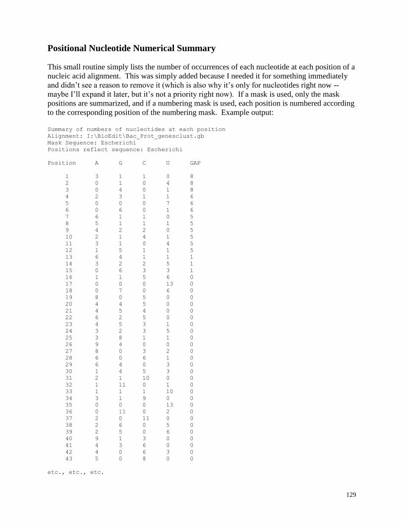
129
Positional Nucleotide Numerical Summary
This small routine simply lists the number of occurrences of each nucleotide at each position of a
nucleic acid alignment. This was simply added because I needed it for something immediately
and didn’t see a reason to remove it (which is also why it’s only for nucleotides right now --
maybe I’ll expand it later, but it’s not a priority right now). If a mask is used, only the mask
positions are summarized, and if a numbering mask is used, each position is numbered according
to the corresponding position of the numbering mask. Example output:
Summary of numbers of nucleotides at each position
Alignment: I:\BioEdit\Bac_Prot_genesclust.gb
Mask Sequence: Escherichi
Positions reflect sequence: Escherichi
Position A G C U GAP
1 3 1 1 0 8
2 0 1 0 4 8
3 0 4 0 1 8
4 2 3 1 1 6
5 0 0 0 7 6
6 0 6 0 1 6
7 6 1 1 0 5
8 5 1 1 1 5
9 4 2 2 0 5
10 2 1 4 1 5
11 3 1 0 4 5
12 1 5 1 1 5
13 6 4 1 1 1
14 3 2 2 5 1
15 0 6 3 3 1
16 1 1 5 6 0
17 0 0 0 13 0
18 0 7 0 6 0
19 8 0 5 0 0
20 4 4 5 0 0
21 4 5 4 0 0
22 6 2 5 0 0
23 4 5 3 1 0
24 3 2 3 5 0
25 3 8 1 1 0
26 9 4 0 0 0
27 8 0 3 2 0
28 6 0 6 1 0
29 6 4 0 3 0
30 1 4 5 3 0
31 2 1 10 0 0
32 1 11 0 1 0
33 1 1 1 10 0
34 3 1 9 0 0
35 0 0 0 13 0
36 0 11 0 2 0
37 2 0 11 0 0
38 2 6 0 5 0
39 2 5 0 6 0
40 9 1 3 0 0
41 4 3 6 0 0
42 4 0 6 3 0
43 5 0 8 0 0
etc., etc., etc.
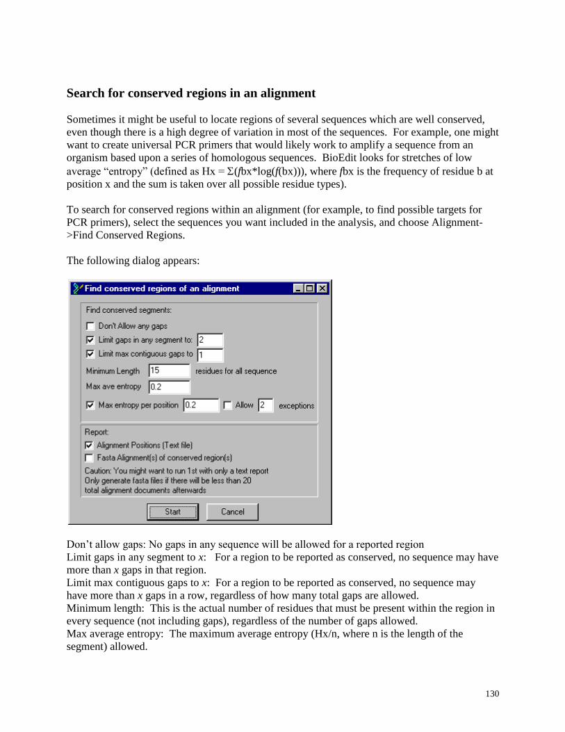
130
Search for conserved regions in an alignment
Sometimes it might be useful to locate regions of several sequences which are well conserved,
even though there is a high degree of variation in most of the sequences. For example, one might
want to create universal PCR primers that would likely work to amplify a sequence from an
organism based upon a series of homologous sequences. BioEdit looks for stretches of low
average “entropy” (defined as Hx = (fbx*log(f(bx))), where fbx is the frequency of residue b at
position x and the sum is taken over all possible residue types).
To search for conserved regions within an alignment (for example, to find possible targets for
PCR primers), select the sequences you want included in the analysis, and choose Alignment-
>Find Conserved Regions.
The following dialog appears:
Don’t allow gaps: No gaps in any sequence will be allowed for a reported region
Limit gaps in any segment to x: For a region to be reported as conserved, no sequence may have
more than x gaps in that region.
Limit max contiguous gaps to x: For a region to be reported as conserved, no sequence may
have more than x gaps in a row, regardless of how many total gaps are allowed.
Minimum length: This is the actual number of residues that must be present within the region in
every sequence (not including gaps), regardless of the number of gaps allowed.
Max average entropy: The maximum average entropy (Hx/n, where n is the length of the
segment) allowed.
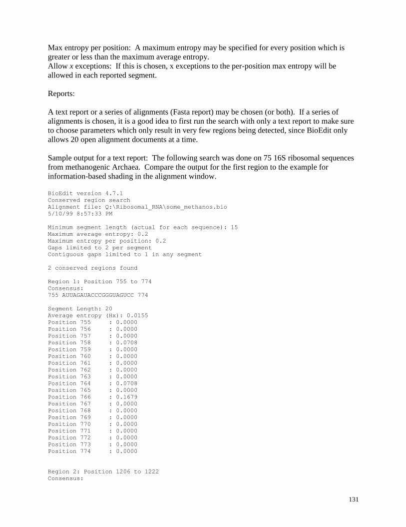
131
Max entropy per position: A maximum entropy may be specified for every position which is
greater or less than the maximum average entropy.
Allow x exceptions: If this is chosen, x exceptions to the per-position max entropy will be
allowed in each reported segment.
Reports:
A text report or a series of alignments (Fasta report) may be chosen (or both). If a series of
alignments is chosen, it is a good idea to first run the search with only a text report to make sure
to choose parameters which only result in very few regions being detected, since BioEdit only
allows 20 open alignment documents at a time.
Sample output for a text report: The following search was done on 75 16S ribosomal sequences
from methanogenic Archaea. Compare the output for the first region to the example for
information-based shading in the alignment window.
BioEdit version 4.7.1
Conserved region search
Alignment file: Q:\Ribosomal_RNA\some_methanos.bio
5/10/99 8:57:33 PM
Minimum segment length (actual for each sequence): 15
Maximum average entropy: 0.2
Maximum entropy per position: 0.2
Gaps limited to 2 per segment
Contiguous gaps limited to 1 in any segment
2 conserved regions found
Region 1: Position 755 to 774
Consensus:
755 AUUAGAUACCCGGGUAGUCC 774
Segment Length: 20
Average entropy (Hx): 0.0155
Position 755 : 0.0000
Position 756 : 0.0000
Position 757 : 0.0000
Position 758 : 0.0708
Position 759 : 0.0000
Position 760 : 0.0000
Position 761 : 0.0000
Position 762 : 0.0000
Position 763 : 0.0000
Position 764 : 0.0708
Position 765 : 0.0000
Position 766 : 0.1679
Position 767 : 0.0000
Position 768 : 0.0000
Position 769 : 0.0000
Position 770 : 0.0000
Position 771 : 0.0000
Position 772 : 0.0000
Position 773 : 0.0000
Position 774 : 0.0000
Region 2: Position 1206 to 1222
Consensus:
132
1206 ACACGCGGGCUACAAUG 1222
Segment Length: 17
Average entropy (Hx): 0.0182
Position 1206 : 0.0000
Position 1207 : 0.0000
Position 1208 : 0.0000
Position 1209 : 0.0000
Position 1210 : 0.0708
Position 1211 : 0.0708
Position 1212 : 0.0000
Position 1213 : 0.1679
Position 1214 : 0.0000
Position 1215 : 0.0000
Position 1216 : 0.0000
Position 1217 : 0.0000
Position 1218 : 0.0000
Position 1219 : 0.0000
Position 1220 : 0.0000
Position 1221 : 0.0000
Position 1222 : 0.0000
A less stringent search might find many regions, for example, for the same alignment:
BioEdit version 4.7.1
Conserved region search
Alignment file: Q:\Ribosomal_RNA\some_methanos.bio
5/10/99 9:34:06 PM
Minimum segment length (actual for each sequence): 10
Maximum average entropy: 0.4
Maximum entropy per position: 0.4 with 2 exceptions allowed
Gaps limited to 2 per segment
Contiguous gaps limited to 1 in any segment
36 conserved regions found ...
and so on ...
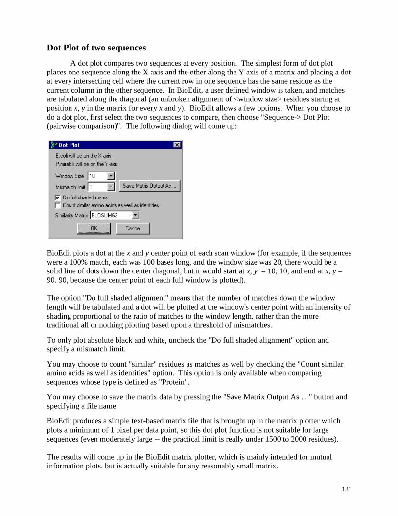
133
Dot Plot of two sequences
A dot plot compares two sequences at every position. The simplest form of dot plot
places one sequence along the X axis and the other along the Y axis of a matrix and placing a dot
at every intersecting cell where the current row in one sequence has the same residue as the
current column in the other sequence. In BioEdit, a user defined window is taken, and matches
are tabulated along the diagonal (an unbroken alignment of <window size> residues staring at
position x, y in the matrix for every x and y). BioEdit allows a few options. When you choose to
do a dot plot, first select the two sequences to compare, then choose "Sequence-> Dot Plot
(pairwise comparison)". The following dialog will come up:
BioEdit plots a dot at the x and y center point of each scan window (for example, if the sequences
were a 100% match, each was 100 bases long, and the window size was 20, there would be a
solid line of dots down the center diagonal, but it would start at x, y = 10, 10, and end at x, y =
90. 90, because the center point of each full window is plotted).
The option "Do full shaded alignment" means that the number of matches down the window
length will be tabulated and a dot will be plotted at the window's center point with an intensity of
shading proportional to the ratio of matches to the window length, rather than the more
traditional all or nothing plotting based upon a threshold of mismatches.
To only plot absolute black and white, uncheck the "Do full shaded alignment" option and
specify a mismatch limit.
You may choose to count "similar" residues as matches as well by checking the "Count similar
amino acids as well as identities" option. This option is only available when comparing
sequences whose type is defined as "Protein".
You may choose to save the matrix data by pressing the "Save Matrix Output As ... " button and
specifying a file name.
BioEdit produces a simple text-based matrix file that is brought up in the matrix plotter which
plots a minimum of 1 pixel per data point, so this dot plot function is not suitable for large
sequences (even moderately large -- the practical limit is really under 1500 to 2000 residues).
The results will come up in the BioEdit matrix plotter, which is mainly intended for mutual
information plots, but is actually suitable for any reasonably small matrix.
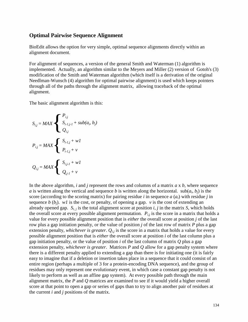
134
Optimal Pairwise Sequence Alignment
BioEdit allows the option for very simple, optimal sequence alignments directly within an
alignment document.
For alignment of sequences, a version of the general Smith and Waterman (1) algorithm is
implemented. Actually, an algorithm similar to the Meyers and Miller (2) version of Gotoh's (3)
modification of the Smith and Waterman algorithm (which itself is a derivation of the original
Needlman-Wunsch (4) algorithm for optimal pairwise alignment) is used which keeps pointers
through all of the paths through the alignment matrix, allowing traceback of the optimal
alignment.
The basic alignment algorithm is this:
{Si,j = MAX
Pi,j
Qi,j
Si-1,j-1 + sub(ai, bj)
{Pi,j = MAXSi-1,j + w1
Pi-1,j + v
{Qi,j = MAXSi,j-1 + w1
Qi,j-1 + v
In the above algorithm, i and j represent the rows and columns of a matrix a x b, where sequence
a is written along the vertical and sequence b is written along the horizontal. sub(ai, bj) is the
score (according to the scoring matrix) for pairing residue i in sequence a (ai) with residue j in
sequence b (bj). w1 is the cost, or penalty, of opening a gap. v is the cost of extending an
already opened gap. Si, j is the total alignment score at position i, j in the matrix S, which holds
the overall score at every possible alignment permutation. Pi,j is the score in a matrix that holds a
value for every possible alignment position that is either the overall score at position j of the last
row plus a gap initiation penalty, or the value of position j of the last row of matrix P plus a gap
extension penalty, whichever is greater. Qi,j is the score in a matrix that holds a value for every
possible alignment position that is either the overall score at position i of the last column plus a
gap initiation penalty, or the value of position i of the last column of matrix Q plus a gap
extension penalty, whichever is greater. Matrices P and Q allow for a gap penalty system where
there is a different penalty applied to extending a gap than there is for initiating one (it is fairly
easy to imagine that if a deletion or insertion takes place in a sequence that it could consist of an
entire region (perhaps a multiple of 3 for a protein-encoding DNA sequence), and the group of
residues may only represent one evolutionary event, in which case a constant gap penalty is not
likely to perform as well as an affine gap system). At every possible path through the main
alignment matrix, the P and Q matrices are examined to see if it would yield a higher overall
score at that point to open a gap or series of gaps than to try to align another pair of residues at
the current i and j positions of the matrix.
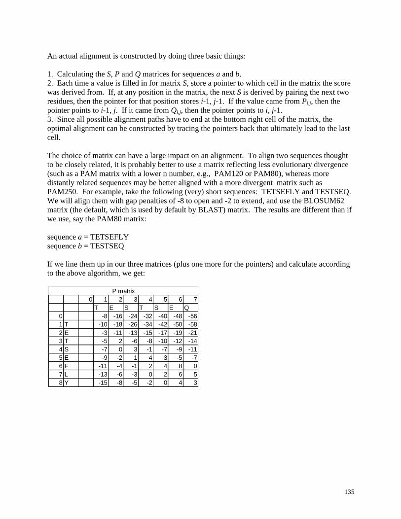
135
An actual alignment is constructed by doing three basic things:
1. Calculating the S, P and Q matrices for sequences a and b.
2. Each time a value is filled in for matrix S, store a pointer to which cell in the matrix the score
was derived from. If, at any position in the matrix, the next S is derived by pairing the next two
residues, then the pointer for that position stores i-1, j-1. If the value came from Pi,j, then the
pointer points to i-1, j. If it came from Qi,j, then the pointer points to i, j-1.
3. Since all possible alignment paths have to end at the bottom right cell of the matrix, the
optimal alignment can be constructed by tracing the pointers back that ultimately lead to the last
cell.
The choice of matrix can have a large impact on an alignment. To align two sequences thought
to be closely related, it is probably better to use a matrix reflecting less evolutionary divergence
(such as a PAM matrix with a lower n number, e.g., PAM120 or PAM80), whereas more
distantly related sequences may be better aligned with a more divergent matrix such as
PAM250. For example, take the following (very) short sequences: TETSEFLY and TESTSEQ.
We will align them with gap penalties of -8 to open and -2 to extend, and use the BLOSUM62
matrix (the default, which is used by default by BLAST) matrix. The results are different than if
we use, say the PAM80 matrix:
sequence a = TETSEFLY
sequence b = TESTSEQ
If we line them up in our three matrices (plus one more for the pointers) and calculate according
to the above algorithm, we get:
0 1 2 3 4 5 6 7
T E S T S E Q
0 -8 -16 -24 -32 -40 -48 -56
1 T -10 -18 -26 -34 -42 -50 -58
2 E -3 -11 -13 -15 -17 -19 -21
3 T -5 2 -6 -8 -10 -12 -14
4 S -7 0 3 -1 -7 -9 -11
5 E -9 -2 1 4 3 -5 -7
6 F -11 -4 -1 2 4 8 0
7 L -13 -6 -3 0 2 6 5
8 Y -15 -8 -5 -2 0 4 3
P matrix
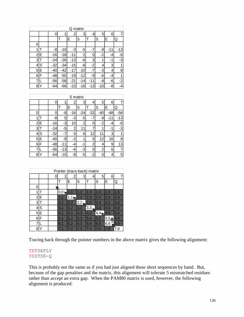
136
Tracing back through the pointer numbers in the above matrix gives the following alignment:
TETSEFLY
TESTSE-Q
This is probably not the same as if you had just aligned these short sequences by hand. But,
because of the gap penalties and the matrix, this alignment will tolerate 5 mismatched residues
rather than accept an extra gap. When the PAM80 matrix is used, however, the following
alignment is produced:
0 1 2 3 4 5 6 7
T E S T S E Q
0
1 T -8 -10 -3 -5 -7 -9 -11 -13
2 E -16 -18 -11 2 0 -2 -4 -6
3 T -24 -26 -13 -6 3 1 -1 -3
4 S -32 -34 -15 -8 -2 4 3 1
5 E -40 -42 -17 -10 -7 -3 4 8
6 F -48 -50 -19 -12 -9 -6 -4 1
7 L -56 -58 -21 -14 -11 -8 -6 -2
8 Y -64 -66 -23 -16 -13 -10 -8 -4
Q matrix
0 1 2 3 4 5 6 7
T E S T S E Q
0 0 -8 -16 -24 -32 -40 -48 -56
1 T -8 5 -3 -5 -7 -9 -11 -13
2 E -16 -3 10 2 0 -2 -4 -6
3 T -24 -5 2 11 7 1 -1 -3
4 S -32 -7 0 6 12 11 3 1
5 E -40 -9 -2 1 5 12 16 8
6 F -48 -11 -4 -1 2 4 9 13
7 L -56 -13 -6 -3 0 2 6 7
8 Y -64 -15 -8 -5 -2 0 4 5
S matrix
0 1 2 3 4 5 6 7
T E S T S E Q
0
1 T 0,0 1,1 1,2 1,3 1,4 1,5 1,6
2 E 1,1 1,1 2,2 2,3 2,4 1,5 2,6
3 T 2,1 2,2 2,2 2,3 2,4 3,5 3,6
4 S 3,1 3,2 3,2 3,3 3,3 4,5 4,6
5 E 4,1 4,1 4,3 4,3 4,4 4,5 5,6
6 F 5,1 5,2 5,3 5,4 5,5 5,5 5,6
7 L 6,1 6,2 6,3 6,4 6,5 6,6 6,5
8 Y 7,1 7,2 7,3 7,4 7,5 7,6 7,6
Pointer (trace-back) matrix
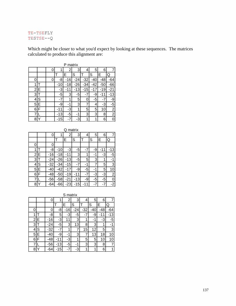
137
TE-TSEFLY
TESTSE--Q
Which might be closer to what you'd expect by looking at these sequences. The matrices
calculated to produce this alignment are:
P matrix
0 1 2 3 4 5 6 7
T E S T S E Q
0 0 -8 -16 -24 -32 -40 -48 -64
1 T -10 -18 -26 -34 -42 -50 -66
2 E -3 -11 -13 -15 -17 -19 -21
3 T -5 3 -5 -7 -9 -11 -13
4 S -7 1 5 0 -5 -7 -9
5 E -9 -1 3 7 4 -3 -5
6 F -11 -3 1 5 5 10 2
7 L -13 -5 -1 3 3 8 2
8 Y -15 -7 -3 1 1 6 0
Q matrix
0 1 2 3 4 5 6 7
T E S T S E Q
0 0
1 T -8 -10 -3 -5 -7 -9 -11 -13
2 E -16 -18 -11 3 1 -1 -3 -5
3 T -24 -26 -13 -5 5 3 1 -1
4 S -32 -34 -15 -7 -1 7 5 3
5 E -40 -42 -17 -9 -5 -1 5 10
6 F -48 -50 -19 -11 -7 -3 -3 2
7 L -56 -58 -21 -13 -9 -5 -5 0
8 Y -64 -66 -23 -15 -11 -7 -7 -2
S matrix
0 1 2 3 4 5 6 7
T E S T S E Q
0 0 -8 -16 -24 -32 -40 -48 -64
1 T -8 5 -3 -5 -7 -9 -11 -13
2 E -16 -3 11 3 1 -1 -3 -5
3 T -24 -5 3 13 8 3 1 -1
4 S -32 -7 1 7 15 12 5 3
5 E -40 -9 -1 3 7 13 18 10
6 F -48 -11 -3 1 5 5 10 10
7 L -56 -13 -5 -1 3 3 8 7
8 Y -64 -15 -7 -3 1 1 6 1
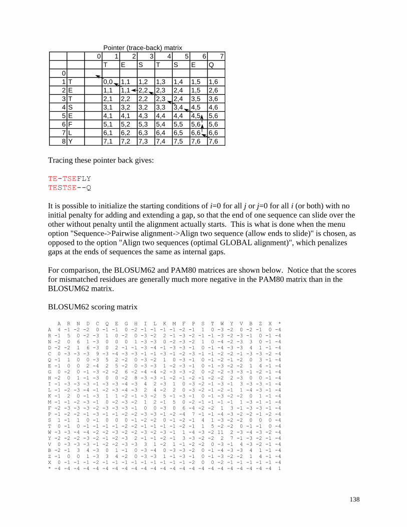
138
Tracing these pointer back gives:
TE-TSEFLY
TESTSE--Q
It is possible to initialize the starting conditions of i=0 for all j or j=0 for all i (or both) with no
initial penalty for adding and extending a gap, so that the end of one sequence can slide over the
other without penalty until the alignment actually starts. This is what is done when the menu
option "Sequence->Pairwise alignment->Align two sequence (allow ends to slide)" is chosen, as
opposed to the option "Align two sequences (optimal GLOBAL alignment)", which penalizes
gaps at the ends of sequences the same as internal gaps.
For comparison, the BLOSUM62 and PAM80 matrices are shown below. Notice that the scores
for mismatched residues are generally much more negative in the PAM80 matrix than in the
BLOSUM62 matrix.
BLOSUM62 scoring matrix
A R N D C Q E G H I L K M F P S T W Y V B Z X *
A 4 -1 -2 -2 0 -1 -1 0 -2 -1 -1 -1 -1 -2 -1 1 0 -3 -2 0 -2 -1 0 -4
R -1 5 0 -2 -3 1 0 -2 0 -3 -2 2 -1 -3 -2 -1 -1 -3 -2 -3 -1 0 -1 -4
N -2 0 6 1 -3 0 0 0 1 -3 -3 0 -2 -3 -2 1 0 -4 -2 -3 3 0 -1 -4
D -2 -2 1 6 -3 0 2 -1 -1 -3 -4 -1 -3 -3 -1 0 -1 -4 -3 -3 4 1 -1 -4
C 0 -3 -3 -3 9 -3 -4 -3 -3 -1 -1 -3 -1 -2 -3 -1 -1 -2 -2 -1 -3 -3 -2 -4
Q -1 1 0 0 -3 5 2 -2 0 -3 -2 1 0 -3 -1 0 -1 -2 -1 -2 0 3 -1 -4
E -1 0 0 2 -4 2 5 -2 0 -3 -3 1 -2 -3 -1 0 -1 -3 -2 -2 1 4 -1 -4
G 0 -2 0 -1 -3 -2 -2 6 -2 -4 -4 -2 -3 -3 -2 0 -2 -2 -3 -3 -1 -2 -1 -4
H -2 0 1 -1 -3 0 0 -2 8 -3 -3 -1 -2 -1 -2 -1 -2 -2 2 -3 0 0 -1 -4
I -1 -3 -3 -3 -1 -3 -3 -4 -3 4 2 -3 1 0 -3 -2 -1 -3 -1 3 -3 -3 -1 -4
L -1 -2 -3 -4 -1 -2 -3 -4 -3 2 4 -2 2 0 -3 -2 -1 -2 -1 1 -4 -3 -1 -4
K -1 2 0 -1 -3 1 1 -2 -1 -3 -2 5 -1 -3 -1 0 -1 -3 -2 -2 0 1 -1 -4
M -1 -1 -2 -3 -1 0 -2 -3 -2 1 2 -1 5 0 -2 -1 -1 -1 -1 1 -3 -1 -1 -4
F -2 -3 -3 -3 -2 -3 -3 -3 -1 0 0 -3 0 6 -4 -2 -2 1 3 -1 -3 -3 -1 -4
P -1 -2 -2 -1 -3 -1 -1 -2 -2 -3 -3 -1 -2 -4 7 -1 -1 -4 -3 -2 -2 -1 -2 -4
S 1 -1 1 0 -1 0 0 0 -1 -2 -2 0 -1 -2 -1 4 1 -3 -2 -2 0 0 0 -4
T 0 -1 0 -1 -1 -1 -1 -2 -2 -1 -1 -1 -1 -2 -1 1 5 -2 -2 0 -1 -1 0 -4
W -3 -3 -4 -4 -2 -2 -3 -2 -2 -3 -2 -3 -1 1 -4 -3 -2 11 2 -3 -4 -3 -2 -4
Y -2 -2 -2 -3 -2 -1 -2 -3 2 -1 -1 -2 -1 3 -3 -2 -2 2 7 -1 -3 -2 -1 -4
V 0 -3 -3 -3 -1 -2 -2 -3 -3 3 1 -2 1 -1 -2 -2 0 -3 -1 4 -3 -2 -1 -4
B -2 -1 3 4 -3 0 1 -1 0 -3 -4 0 -3 -3 -2 0 -1 -4 -3 -3 4 1 -1 -4
Z -1 0 0 1 -3 3 4 -2 0 -3 -3 1 -1 -3 -1 0 -1 -3 -2 -2 1 4 -1 -4
X 0 -1 -1 -1 -2 -1 -1 -1 -1 -1 -1 -1 -1 -1 -2 0 0 -2 -1 -1 -1 -1 -1 -4
* -4 -4 -4 -4 -4 -4 -4 -4 -4 -4 -4 -4 -4 -4 -4 -4 -4 -4 -4 -4 -4 -4 -4 1
Pointer (trace-back) matrix
0 1 2 3 4 5 6 7
T E S T S E Q
0
1 T 0,0 1,1 1,2 1,3 1,4 1,5 1,6
2 E 1,1 1,1 2,2 2,3 2,4 1,5 2,6
3 T 2,1 2,2 2,2 2,3 2,4 3,5 3,6
4 S 3,1 3,2 3,2 3,3 3,4 4,5 4,6
5 E 4,1 4,1 4,3 4,4 4,4 4,5 5,6
6 F 5,1 5,2 5,3 5,4 5,5 5,6 5,6
7 L 6,1 6,2 6,3 6,4 6,5 6,6 6,6
8 Y 7,1 7,2 7,3 7,4 7,5 7,6 7,6
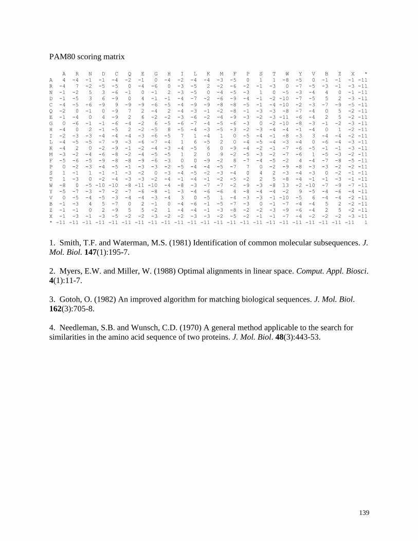
139
PAM80 scoring matrix
A R N D C Q E G H I L K M F P S T W Y V B Z X *
A 4 -4 -1 -1 -4 -2 -1 0 -4 -2 -4 -4 -3 -5 0 1 1 -8 -5 0 -1 -1 -1 -11
R -4 7 -2 -5 -5 0 -4 -6 0 -3 -5 2 -2 -6 -2 -1 -3 0 -7 -5 -3 -1 -3 -11
N -1 -2 5 3 -6 -1 0 -1 2 -3 -5 0 -4 -5 -3 1 0 -5 -3 -4 4 0 -1 -11
D -1 -5 3 6 -9 0 4 -1 -1 -4 -7 -2 -6 -9 -4 -1 -2 -10 -7 -5 5 2 -3 -11
C -4 -5 -6 -9 9 -9 -9 -6 -5 -4 -9 -9 -8 -8 -5 -1 -4 -10 -2 -3 -7 -9 -5 -11
Q -2 0 -1 0 -9 7 2 -4 2 -4 -3 -1 -2 -8 -1 -3 -3 -8 -7 -4 0 5 -2 -11
E -1 -4 0 4 -9 2 6 -2 -2 -3 -6 -2 -4 -9 -3 -2 -3 -11 -6 -4 2 5 -2 -11
G 0 -6 -1 -1 -6 -4 -2 6 -5 -6 -7 -4 -5 -6 -3 0 -2 -10 -8 -3 -1 -2 -3 -11
H -4 0 2 -1 -5 2 -2 -5 8 -5 -4 -3 -5 -3 -2 -3 -4 -4 -1 -4 0 1 -2 -11
I -2 -3 -3 -4 -4 -4 -3 -6 -5 7 1 -4 1 0 -5 -4 -1 -8 -3 3 -4 -4 -2 -11
L -4 -5 -5 -7 -9 -3 -6 -7 -4 1 6 -5 2 0 -4 -5 -4 -3 -4 0 -6 -4 -3 -11
K -4 2 0 -2 -9 -1 -2 -4 -3 -4 -5 6 0 -9 -4 -2 -1 -7 -6 -5 -1 -1 -3 -11
M -3 -2 -4 -6 -8 -2 -4 -5 -5 1 2 0 9 -2 -5 -3 -2 -7 -6 1 -5 -3 -2 -11
F -5 -6 -5 -9 -8 -8 -9 -6 -3 0 0 -9 -2 8 -7 -4 -5 -2 4 -4 -7 -8 -5 -11
P 0 -2 -3 -4 -5 -1 -3 -3 -2 -5 -4 -4 -5 -7 7 0 -2 -9 -8 -3 -3 -2 -2 -11
S 1 -1 1 -1 -1 -3 -2 0 -3 -4 -5 -2 -3 -4 0 4 2 -3 -4 -3 0 -2 -1 -11
T 1 -3 0 -2 -4 -3 -3 -2 -4 -1 -4 -1 -2 -5 -2 2 5 -8 -4 -1 -1 -3 -1 -11
W -8 0 -5 -10 -10 -8 -11 -10 -4 -8 -3 -7 -7 -2 -9 -3 -8 13 -2 -10 -7 -9 -7 -11
Y -5 -7 -3 -7 -2 -7 -6 -8 -1 -3 -4 -6 -6 4 -8 -4 -4 -2 9 -5 -4 -6 -4 -11
V 0 -5 -4 -5 -3 -4 -4 -3 -4 3 0 -5 1 -4 -3 -3 -1 -10 -5 6 -4 -4 -2 -11
B -1 -3 4 5 -7 0 2 -1 0 -4 -6 -1 -5 -7 -3 0 -1 -7 -4 -4 5 2 -2 -11
Z -1 -1 0 2 -9 5 5 -2 1 -4 -4 -1 -3 -8 -2 -2 -3 -9 -6 -4 2 5 -2 -11
X -1 -3 -1 -3 -5 -2 -2 -3 -2 -2 -3 -3 -2 -5 -2 -1 -1 -7 -4 -2 -2 -2 -3 -11
* -11 -11 -11 -11 -11 -11 -11 -11 -11 -11 -11 -11 -11 -11 -11 -11 -11 -11 -11 -11 -11 -11 -11 1
1. Smith, T.F. and Waterman, M.S. (1981) Identification of common molecular subsequences. J.
Mol. Biol. 147(1):195-7.
2. Myers, E.W. and Miller, W. (1988) Optimal alignments in linear space. Comput. Appl. Biosci.
4(1):11-7.
3. Gotoh, O. (1982) An improved algorithm for matching biological sequences. J. Mol. Biol.
162(3):705-8.
4. Needleman, S.B. and Wunsch, C.D. (1970) A general method applicable to the search for
similarities in the amino acid sequence of two proteins. J. Mol. Biol. 48(3):443-53.
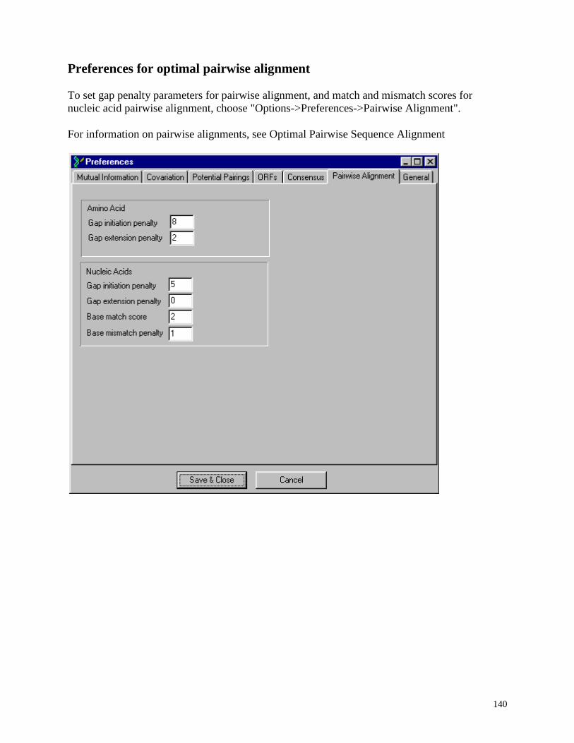
140
Preferences for optimal pairwise alignment
To set gap penalty parameters for pairwise alignment, and match and mismatch scores for
nucleic acid pairwise alignment, choose "Options->Preferences->Pairwise Alignment".
For information on pairwise alignments, see Optimal Pairwise Sequence Alignment
141
Substitution Matrices used for pairwise alignment and alignment shading
When trying to construct the most likely alignment between two (or more) sequences
assumed to be homologous (i.e., derived from the same ancestral sequence), criteria are needed
to specify the level of "similarity" between two aligned residues in order to assess their
contribution to the quality of the overall alignment. Although the level of similarity between two
residues is not literally meaningful (they are either identical or not, and they either occupy a
position in each respective sequence that is the same relative to the ancestral sequence, or they
do not), we do not have the data for the ancestral sequence(s) nor the evolutionary steps that led
to the current sequences, and we need a system that allows us to estimate the likelihood that one
residue has been substituted for another through natural selection (some reflection of the
frequency we can expect to see residue a substituted for residue b). A collection of similarity
values that compares every combination of available residues is called a substitution matrix. For
a general introduction to the generation of scoring matrices and basic sequence alignment, I
would recommend reference 1 (below)
BioEdit provides a small collection of common substitution matrices for optimal pairwise
alignment and for shading similar amino acids in the alignment document view and in the
graphic alignment view.
The following matrices are provided and can be found in the BioEdit/apps folder in plain text
format:
BLOSUM62: A commonly used matrix developed by Henikoff and Henikoff (2), which is
suggested to be more sensitive than the older PAM matrices (3) for database searching (4) and is
the default matrix used by the NCBI BLAST program.
The BLOSUM62 matrix supplied with BioEdit 5.0.0 was obtained from:
ftp://ncbi.nlm.nih.gov/repository/blocks/unix/blosum/BLOSUM/blosum62.bla
PAM40, PAM80, PAM120 and PAM250: Current PAM matrices, as generated by the PAM
program -- see:
http://www.cmbi.kun.nl/bioinf/tools/pam.shtml
PAM is an acronym for "Point Accepted Mutation" (3). One PAM unit is the evolutionary
"time", or divergence, that results in 1 amino acid substitution per 100 amino acids of protein on
average (1%). Larger PAM values indicate greater evolutionary divergence. The PAM matrices
were derived from alignments of closely related amino acid sequences, then extrapolated to
reflect evolutionary times of n PAM units for a PAMn matrix (the PAM120 matrix gives an
indication of the relative expected substitutions frequencies of all residue combinations in 120
PAM units of evolutionary distance). The number scores in these matrices are the "log odds"
ratio of the frequency observed of each substitution (in a given amount of evolutionary "time") to
the probability of finding the match randomly, or log(qn
a,b/pa,pb), where qa,b is the observed
frequency of a substitution in n units of evolution of residue a to residue b, and pa and pb are the
individual probabilities of finding residue a and b, respectively. The PAM250 matrix, then,
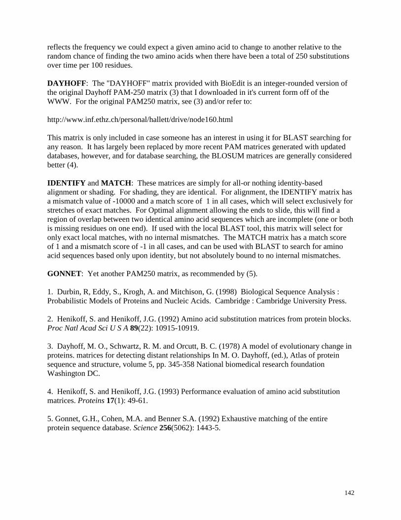
142
reflects the frequency we could expect a given amino acid to change to another relative to the
random chance of finding the two amino acids when there have been a total of 250 substitutions
over time per 100 residues.
DAYHOFF: The "DAYHOFF" matrix provided with BioEdit is an integer-rounded version of
the original Dayhoff PAM-250 matrix (3) that I downloaded in it's current form off of the
WWW. For the original PAM250 matrix, see (3) and/or refer to:
http://www.inf.ethz.ch/personal/hallett/drive/node160.html
This matrix is only included in case someone has an interest in using it for BLAST searching for
any reason. It has largely been replaced by more recent PAM matrices generated with updated
databases, however, and for database searching, the BLOSUM matrices are generally considered
better (4).
IDENTIFY and MATCH: These matrices are simply for all-or nothing identity-based
alignment or shading. For shading, they are identical. For alignment, the IDENTIFY matrix has
a mismatch value of -10000 and a match score of 1 in all cases, which will select exclusively for
stretches of exact matches. For Optimal alignment allowing the ends to slide, this will find a
region of overlap between two identical amino acid sequences which are incomplete (one or both
is missing residues on one end). If used with the local BLAST tool, this matrix will select for
only exact local matches, with no internal mismatches. The MATCH matrix has a match score
of 1 and a mismatch score of -1 in all cases, and can be used with BLAST to search for amino
acid sequences based only upon identity, but not absolutely bound to no internal mismatches.
GONNET: Yet another PAM250 matrix, as recommended by (5).
1. Durbin, R, Eddy, S., Krogh, A. and Mitchison, G. (1998) Biological Sequence Analysis :
Probabilistic Models of Proteins and Nucleic Acids. Cambridge : Cambridge University Press.
2. Henikoff, S. and Henikoff, J.G. (1992) Amino acid substitution matrices from protein blocks.
Proc Natl Acad Sci U S A 89(22): 10915-10919.
3. Dayhoff, M. O., Schwartz, R. M. and Orcutt, B. C. (1978) A model of evolutionary change in
proteins. matrices for detecting distant relationships In M. O. Dayhoff, (ed.), Atlas of protein
sequence and structure, volume 5, pp. 345-358 National biomedical research foundation
Washington DC.
4. Henikoff, S. and Henikoff, J.G. (1993) Performance evaluation of amino acid substitution
matrices. Proteins 17(1): 49-61.
5. Gonnet, G.H., Cohen, M.A. and Benner S.A. (1992) Exhaustive matching of the entire
protein sequence database. Science 256(5062): 1443-5.
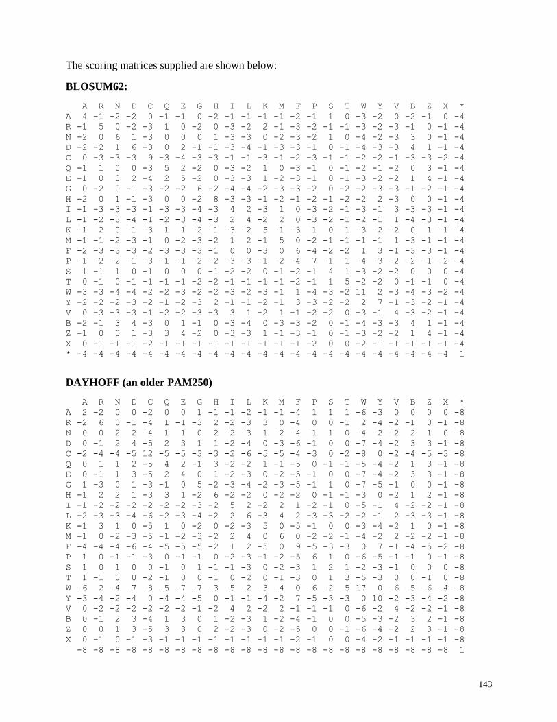
143
The scoring matrices supplied are shown below:
BLOSUM62:
A R N D C Q E G H I L K M F P S T W Y V B Z X *
A 4 -1 -2 -2 0 -1 -1 0 -2 -1 -1 -1 -1 -2 -1 1 0 -3 -2 0 -2 -1 0 -4
R -1 5 0 -2 -3 1 0 -2 0 -3 -2 2 -1 -3 -2 -1 -1 -3 -2 -3 -1 0 -1 -4
N -2 0 6 1 -3 0 0 0 1 -3 -3 0 -2 -3 -2 1 0 -4 -2 -3 3 0 -1 -4
D -2 -2 1 6 -3 0 2 -1 -1 -3 -4 -1 -3 -3 -1 0 -1 -4 -3 -3 4 1 -1 -4
C 0 -3 -3 -3 9 -3 -4 -3 -3 -1 -1 -3 -1 -2 -3 -1 -1 -2 -2 -1 -3 -3 -2 -4
Q -1 1 0 0 -3 5 2 -2 0 -3 -2 1 0 -3 -1 0 -1 -2 -1 -2 0 3 -1 -4
E -1 0 0 2 -4 2 5 -2 0 -3 -3 1 -2 -3 -1 0 -1 -3 -2 -2 1 4 -1 -4
G 0 -2 0 -1 -3 -2 -2 6 -2 -4 -4 -2 -3 -3 -2 0 -2 -2 -3 -3 -1 -2 -1 -4
H -2 0 1 -1 -3 0 0 -2 8 -3 -3 -1 -2 -1 -2 -1 -2 -2 2 -3 0 0 -1 -4
I -1 -3 -3 -3 -1 -3 -3 -4 -3 4 2 -3 1 0 -3 -2 -1 -3 -1 3 -3 -3 -1 -4
L -1 -2 -3 -4 -1 -2 -3 -4 -3 2 4 -2 2 0 -3 -2 -1 -2 -1 1 -4 -3 -1 -4
K -1 2 0 -1 -3 1 1 -2 -1 -3 -2 5 -1 -3 -1 0 -1 -3 -2 -2 0 1 -1 -4
M -1 -1 -2 -3 -1 0 -2 -3 -2 1 2 -1 5 0 -2 -1 -1 -1 -1 1 -3 -1 -1 -4
F -2 -3 -3 -3 -2 -3 -3 -3 -1 0 0 -3 0 6 -4 -2 -2 1 3 -1 -3 -3 -1 -4
P -1 -2 -2 -1 -3 -1 -1 -2 -2 -3 -3 -1 -2 -4 7 -1 -1 -4 -3 -2 -2 -1 -2 -4
S 1 -1 1 0 -1 0 0 0 -1 -2 -2 0 -1 -2 -1 4 1 -3 -2 -2 0 0 0 -4
T 0 -1 0 -1 -1 -1 -1 -2 -2 -1 -1 -1 -1 -2 -1 1 5 -2 -2 0 -1 -1 0 -4
W -3 -3 -4 -4 -2 -2 -3 -2 -2 -3 -2 -3 -1 1 -4 -3 -2 11 2 -3 -4 -3 -2 -4
Y -2 -2 -2 -3 -2 -1 -2 -3 2 -1 -1 -2 -1 3 -3 -2 -2 2 7 -1 -3 -2 -1 -4
V 0 -3 -3 -3 -1 -2 -2 -3 -3 3 1 -2 1 -1 -2 -2 0 -3 -1 4 -3 -2 -1 -4
B -2 -1 3 4 -3 0 1 -1 0 -3 -4 0 -3 -3 -2 0 -1 -4 -3 -3 4 1 -1 -4
Z -1 0 0 1 -3 3 4 -2 0 -3 -3 1 -1 -3 -1 0 -1 -3 -2 -2 1 4 -1 -4
X 0 -1 -1 -1 -2 -1 -1 -1 -1 -1 -1 -1 -1 -1 -2 0 0 -2 -1 -1 -1 -1 -1 -4
* -4 -4 -4 -4 -4 -4 -4 -4 -4 -4 -4 -4 -4 -4 -4 -4 -4 -4 -4 -4 -4 -4 -4 1
DAYHOFF (an older PAM250)
A R N D C Q E G H I L K M F P S T W Y V B Z X *
A 2 -2 0 0 -2 0 0 1 -1 -1 -2 -1 -1 -4 1 1 1 -6 -3 0 0 0 0 -8
R -2 6 0 -1 -4 1 -1 -3 2 -2 -3 3 0 -4 0 0 -1 2 -4 -2 -1 0 -1 -8
N 0 0 2 2 -4 1 1 0 2 -2 -3 1 -2 -4 -1 1 0 -4 -2 -2 2 1 0 -8
D 0 -1 2 4 -5 2 3 1 1 -2 -4 0 -3 -6 -1 0 0 -7 -4 -2 3 3 -1 -8
C -2 -4 -4 -5 12 -5 -5 -3 -3 -2 -6 -5 -5 -4 -3 0 -2 -8 0 -2 -4 -5 -3 -8
Q 0 1 1 2 -5 4 2 -1 3 -2 -2 1 -1 -5 0 -1 -1 -5 -4 -2 1 3 -1 -8
E 0 -1 1 3 -5 2 4 0 1 -2 -3 0 -2 -5 -1 0 0 -7 -4 -2 3 3 -1 -8
G 1 -3 0 1 -3 -1 0 5 -2 -3 -4 -2 -3 -5 -1 1 0 -7 -5 -1 0 0 -1 -8
H -1 2 2 1 -3 3 1 -2 6 -2 -2 0 -2 -2 0 -1 -1 -3 0 -2 1 2 -1 -8
I -1 -2 -2 -2 -2 -2 -2 -3 -2 5 2 -2 2 1 -2 -1 0 -5 -1 4 -2 -2 -1 -8
L -2 -3 -3 -4 -6 -2 -3 -4 -2 2 6 -3 4 2 -3 -3 -2 -2 -1 2 -3 -3 -1 -8
K -1 3 1 0 -5 1 0 -2 0 -2 -3 5 0 -5 -1 0 0 -3 -4 -2 1 0 -1 -8
M -1 0 -2 -3 -5 -1 -2 -3 -2 2 4 0 6 0 -2 -2 -1 -4 -2 2 -2 -2 -1 -8
F -4 -4 -4 -6 -4 -5 -5 -5 -2 1 2 -5 0 9 -5 -3 -3 0 7 -1 -4 -5 -2 -8
P 1 0 -1 -1 -3 0 -1 -1 0 -2 -3 -1 -2 -5 6 1 0 -6 -5 -1 -1 0 -1 -8
S 1 0 1 0 0 -1 0 1 -1 -1 -3 0 -2 -3 1 2 1 -2 -3 -1 0 0 0 -8
T 1 -1 0 0 -2 -1 0 0 -1 0 -2 0 -1 -3 0 1 3 -5 -3 0 0 -1 0 -8
W -6 2 -4 -7 -8 -5 -7 -7 -3 -5 -2 -3 -4 0 -6 -2 -5 17 0 -6 -5 -6 -4 -8
Y -3 -4 -2 -4 0 -4 -4 -5 0 -1 -1 -4 -2 7 -5 -3 -3 0 10 -2 -3 -4 -2 -8
V 0 -2 -2 -2 -2 -2 -2 -1 -2 4 2 -2 2 -1 -1 -1 0 -6 -2 4 -2 -2 -1 -8
B 0 -1 2 3 -4 1 3 0 1 -2 -3 1 -2 -4 -1 0 0 -5 -3 -2 3 2 -1 -8
Z 0 0 1 3 -5 3 3 0 2 -2 -3 0 -2 -5 0 0 -1 -6 -4 -2 2 3 -1 -8
X 0 -1 0 -1 -3 -1 -1 -1 -1 -1 -1 -1 -1 -2 -1 0 0 -4 -2 -1 -1 -1 -1 -8
-8 -8 -8 -8 -8 -8 -8 -8 -8 -8 -8 -8 -8 -8 -8 -8 -8 -8 -8 -8 -8 -8 -8 1
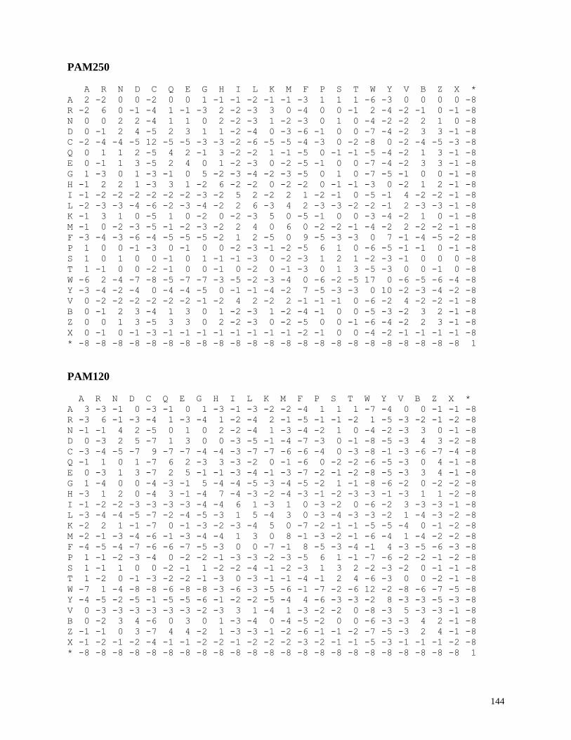
144
PAM250
A R N D C Q E G H I L K M F P S T W Y V B Z X *
A 2 -2 0 0 -2 0 0 1 -1 -1 -2 -1 -1 -3 1 1 1 -6 -3 0 0 0 0 -8
R -2 6 0 -1 -4 1 -1 -3 2 -2 -3 3 0 -4 0 0 -1 2 -4 -2 -1 0 -1 -8
N 0 0 2 2 -4 1 1 0 2 -2 -3 1 -2 -3 0 1 0 -4 -2 -2 2 1 0 -8
D 0 -1 2 4 -5 2 3 1 1 -2 -4 0 -3 -6 -1 0 0 -7 -4 -2 3 3 -1 -8
C -2 -4 -4 -5 12 -5 -5 -3 -3 -2 -6 -5 -5 -4 -3 0 -2 -8 0 -2 -4 -5 -3 -8
Q 0 1 1 2 -5 4 2 -1 3 -2 -2 1 -1 -5 0 -1 -1 -5 -4 -2 1 3 -1 -8
E 0 -1 1 3 -5 2 4 0 1 -2 -3 0 -2 -5 -1 0 0 -7 -4 -2 3 3 -1 -8
G 1 -3 0 1 -3 -1 0 5 -2 -3 -4 -2 -3 -5 0 1 0 -7 -5 -1 0 0 -1 -8
H -1 2 2 1 -3 3 1 -2 6 -2 -2 0 -2 -2 0 -1 -1 -3 0 -2 1 2 -1 -8
I -1 -2 -2 -2 -2 -2 -2 -3 -2 5 2 -2 2 1 -2 -1 0 -5 -1 4 -2 -2 -1 -8
L -2 -3 -3 -4 -6 -2 -3 -4 -2 2 6 -3 4 2 -3 -3 -2 -2 -1 2 -3 -3 -1 -8
K -1 3 1 0 -5 1 0 -2 0 -2 -3 5 0 -5 -1 0 0 -3 -4 -2 1 0 -1 -8
M -1 0 -2 -3 -5 -1 -2 -3 -2 2 4 0 6 0 -2 -2 -1 -4 -2 2 -2 -2 -1 -8
F -3 -4 -3 -6 -4 -5 -5 -5 -2 1 2 -5 0 9 -5 -3 -3 0 7 -1 -4 -5 -2 -8
P 1 0 0 -1 -3 0 -1 0 0 -2 -3 -1 -2 -5 6 1 0 -6 -5 -1 -1 0 -1 -8
S 1 0 1 0 0 -1 0 1 -1 -1 -3 0 -2 -3 1 2 1 -2 -3 -1 0 0 0 -8
T 1 -1 0 0 -2 -1 0 0 -1 0 -2 0 -1 -3 0 1 3 -5 -3 0 0 -1 0 -8
W -6 2 -4 -7 -8 -5 -7 -7 -3 -5 -2 -3 -4 0 -6 -2 -5 17 0 -6 -5 -6 -4 -8
Y -3 -4 -2 -4 0 -4 -4 -5 0 -1 -1 -4 -2 7 -5 -3 -3 0 10 -2 -3 -4 -2 -8
V 0 -2 -2 -2 -2 -2 -2 -1 -2 4 2 -2 2 -1 -1 -1 0 -6 -2 4 -2 -2 -1 -8
B 0 -1 2 3 -4 1 3 0 1 -2 -3 1 -2 -4 -1 0 0 -5 -3 -2 3 2 -1 -8
Z 0 0 1 3 -5 3 3 0 2 -2 -3 0 -2 -5 0 0 -1 -6 -4 -2 2 3 -1 -8
X 0 -1 0 -1 -3 -1 -1 -1 -1 -1 -1 -1 -1 -2 -1 0 0 -4 -2 -1 -1 -1 -1 -8
* -8 -8 -8 -8 -8 -8 -8 -8 -8 -8 -8 -8 -8 -8 -8 -8 -8 -8 -8 -8 -8 -8 -8 1
PAM120
A R N D C Q E G H I L K M F P S T W Y V B Z X *
A 3 -3 -1 0 -3 -1 0 1 -3 -1 -3 -2 -2 -4 1 1 1 -7 -4 0 0 -1 -1 -8
R -3 6 -1 -3 -4 1 -3 -4 1 -2 -4 2 -1 -5 -1 -1 -2 1 -5 -3 -2 -1 -2 -8
N -1 -1 4 2 -5 0 1 0 2 -2 -4 1 -3 -4 -2 1 0 -4 -2 -3 3 0 -1 -8
D 0 -3 2 5 -7 1 3 0 0 -3 -5 -1 -4 -7 -3 0 -1 -8 -5 -3 4 3 -2 -8
C -3 -4 -5 -7 9 -7 -7 -4 -4 -3 -7 -7 -6 -6 -4 0 -3 -8 -1 -3 -6 -7 -4 -8
Q -1 1 0 1 -7 6 2 -3 3 -3 -2 0 -1 -6 0 -2 -2 -6 -5 -3 0 4 -1 -8
E 0 -3 1 3 -7 2 5 -1 -1 -3 -4 -1 -3 -7 -2 -1 -2 -8 -5 -3 3 4 -1 -8
G 1 -4 0 0 -4 -3 -1 5 -4 -4 -5 -3 -4 -5 -2 1 -1 -8 -6 -2 0 -2 -2 -8
H -3 1 2 0 -4 3 -1 -4 7 -4 -3 -2 -4 -3 -1 -2 -3 -3 -1 -3 1 1 -2 -8
I -1 -2 -2 -3 -3 -3 -3 -4 -4 6 1 -3 1 0 -3 -2 0 -6 -2 3 -3 -3 -1 -8
L -3 -4 -4 -5 -7 -2 -4 -5 -3 1 5 -4 3 0 -3 -4 -3 -3 -2 1 -4 -3 -2 -8
K -2 2 1 -1 -7 0 -1 -3 -2 -3 -4 5 0 -7 -2 -1 -1 -5 -5 -4 0 -1 -2 -8
M -2 -1 -3 -4 -6 -1 -3 -4 -4 1 3 0 8 -1 -3 -2 -1 -6 -4 1 -4 -2 -2 -8
F -4 -5 -4 -7 -6 -6 -7 -5 -3 0 0 -7 -1 8 -5 -3 -4 -1 4 -3 -5 -6 -3 -8
P 1 -1 -2 -3 -4 0 -2 -2 -1 -3 -3 -2 -3 -5 6 1 -1 -7 -6 -2 -2 -1 -2 -8
S 1 -1 1 0 0 -2 -1 1 -2 -2 -4 -1 -2 -3 1 3 2 -2 -3 -2 0 -1 -1 -8
T 1 -2 0 -1 -3 -2 -2 -1 -3 0 -3 -1 -1 -4 -1 2 4 -6 -3 0 0 -2 -1 -8
W -7 1 -4 -8 -8 -6 -8 -8 -3 -6 -3 -5 -6 -1 -7 -2 -6 12 -2 -8 -6 -7 -5 -8
Y -4 -5 -2 -5 -1 -5 -5 -6 -1 -2 -2 -5 -4 4 -6 -3 -3 -2 8 -3 -3 -5 -3 -8
V 0 -3 -3 -3 -3 -3 -3 -2 -3 3 1 -4 1 -3 -2 -2 0 -8 -3 5 -3 -3 -1 -8
B 0 -2 3 4 -6 0 3 0 1 -3 -4 0 -4 -5 -2 0 0 -6 -3 -3 4 2 -1 -8
Z -1 -1 0 3 -7 4 4 -2 1 -3 -3 -1 -2 -6 -1 -1 -2 -7 -5 -3 2 4 -1 -8
X -1 -2 -1 -2 -4 -1 -1 -2 -2 -1 -2 -2 -2 -3 -2 -1 -1 -5 -3 -1 -1 -1 -2 -8
* -8 -8 -8 -8 -8 -8 -8 -8 -8 -8 -8 -8 -8 -8 -8 -8 -8 -8 -8 -8 -8 -8 -8 1
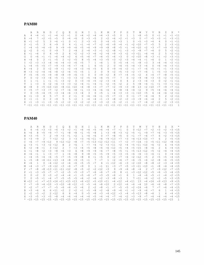
145
PAM80 A R N D C Q E G H I L K M F P S T W Y V B Z X *
A 4 -4 -1 -1 -4 -2 -1 0 -4 -2 -4 -4 -3 -5 0 1 1 -8 -5 0 -1 -1 -1 -11
R -4 7 -2 -5 -5 0 -4 -6 0 -3 -5 2 -2 -6 -2 -1 -3 0 -7 -5 -3 -1 -3 -11
N -1 -2 5 3 -6 -1 0 -1 2 -3 -5 0 -4 -5 -3 1 0 -5 -3 -4 4 0 -1 -11
D -1 -5 3 6 -9 0 4 -1 -1 -4 -7 -2 -6 -9 -4 -1 -2 -10 -7 -5 5 2 -3 -11
C -4 -5 -6 -9 9 -9 -9 -6 -5 -4 -9 -9 -8 -8 -5 -1 -4 -10 -2 -3 -7 -9 -5 -11
Q -2 0 -1 0 -9 7 2 -4 2 -4 -3 -1 -2 -8 -1 -3 -3 -8 -7 -4 0 5 -2 -11
E -1 -4 0 4 -9 2 6 -2 -2 -3 -6 -2 -4 -9 -3 -2 -3 -11 -6 -4 2 5 -2 -11
G 0 -6 -1 -1 -6 -4 -2 6 -5 -6 -7 -4 -5 -6 -3 0 -2 -10 -8 -3 -1 -2 -3 -11
H -4 0 2 -1 -5 2 -2 -5 8 -5 -4 -3 -5 -3 -2 -3 -4 -4 -1 -4 0 1 -2 -11
I -2 -3 -3 -4 -4 -4 -3 -6 -5 7 1 -4 1 0 -5 -4 -1 -8 -3 3 -4 -4 -2 -11
L -4 -5 -5 -7 -9 -3 -6 -7 -4 1 6 -5 2 0 -4 -5 -4 -3 -4 0 -6 -4 -3 -11
K -4 2 0 -2 -9 -1 -2 -4 -3 -4 -5 6 0 -9 -4 -2 -1 -7 -6 -5 -1 -1 -3 -11
M -3 -2 -4 -6 -8 -2 -4 -5 -5 1 2 0 9 -2 -5 -3 -2 -7 -6 1 -5 -3 -2 -11
F -5 -6 -5 -9 -8 -8 -9 -6 -3 0 0 -9 -2 8 -7 -4 -5 -2 4 -4 -7 -8 -5 -11
P 0 -2 -3 -4 -5 -1 -3 -3 -2 -5 -4 -4 -5 -7 7 0 -2 -9 -8 -3 -3 -2 -2 -11
S 1 -1 1 -1 -1 -3 -2 0 -3 -4 -5 -2 -3 -4 0 4 2 -3 -4 -3 0 -2 -1 -11
T 1 -3 0 -2 -4 -3 -3 -2 -4 -1 -4 -1 -2 -5 -2 2 5 -8 -4 -1 -1 -3 -1 -11
W -8 0 -5 -10 -10 -8 -11 -10 -4 -8 -3 -7 -7 -2 -9 -3 -8 13 -2 -10 -7 -9 -7 -11
Y -5 -7 -3 -7 -2 -7 -6 -8 -1 -3 -4 -6 -6 4 -8 -4 -4 -2 9 -5 -4 -6 -4 -11
V 0 -5 -4 -5 -3 -4 -4 -3 -4 3 0 -5 1 -4 -3 -3 -1 -10 -5 6 -4 -4 -2 -11
B -1 -3 4 5 -7 0 2 -1 0 -4 -6 -1 -5 -7 -3 0 -1 -7 -4 -4 5 2 -2 -11
Z -1 -1 0 2 -9 5 5 -2 1 -4 -4 -1 -3 -8 -2 -2 -3 -9 -6 -4 2 5 -2 -11
X -1 -3 -1 -3 -5 -2 -2 -3 -2 -2 -3 -3 -2 -5 -2 -1 -1 -7 -4 -2 -2 -2 -3 -11
* -11 -11 -11 -11 -11 -11 -11 -11 -11 -11 -11 -11 -11 -11 -11 -11 -11 -11 -11 -11 -11 -11 -11 1
PAM40
A R N D C Q E G H I L K M F P S T W Y V B Z X *
A 6 -6 -3 -3 -6 -3 -2 -1 -6 -4 -5 -6 -4 -7 -1 0 0 -12 -7 -2 -3 -2 -3 -15
R -6 8 -5 -9 -7 -1 -8 -8 -1 -5 -8 1 -3 -8 -3 -2 -5 -1 -9 -7 -6 -3 -5 -15
N -3 -5 7 2 -9 -3 -1 -2 1 -4 -6 0 -7 -8 -5 0 -1 -7 -4 -7 6 -2 -3 -15
D -3 -9 2 7 -12 -2 3 -3 -3 -6 -11 -4 -9 -13 -7 -3 -4 -13 -10 -7 6 2 -5 -15
C -6 -7 -9 -12 9 -12 -12 -8 -7 -5 -13 -12 -12 -11 -7 -2 -7 -14 -3 -5 -11 -12 -8 -15
Q -3 -1 -3 -2 -12 8 2 -6 1 -7 -4 -2 -3 -11 -2 -4 -5 -11 -10 -6 -2 6 -4 -15
E -2 -8 -1 3 -12 2 7 -3 -4 -5 -8 -4 -6 -12 -5 -4 -5 -15 -8 -6 2 6 -4 -15
G -1 -8 -2 -3 -8 -6 -3 6 -8 -9 -9 -6 -7 -8 -5 -1 -5 -13 -12 -5 -2 -4 -4 -15
H -6 -1 1 -3 -7 1 -4 -8 9 -8 -5 -5 -9 -5 -3 -5 -6 -6 -3 -6 -1 0 -4 -15
I -4 -5 -4 -6 -5 -7 -5 -9 -8 8 -1 -5 0 -2 -7 -6 -2 -12 -5 2 -5 -5 -4 -15
L -5 -8 -6 -11 -13 -4 -8 -9 -5 -1 7 -7 1 -2 -6 -7 -6 -5 -6 -2 -8 -6 -5 -15
K -6 1 0 -4 -12 -2 -4 -6 -5 -5 -7 6 -1 -12 -6 -3 -2 -10 -8 -8 -2 -3 -4 -15
M -4 -3 -7 -9 -12 -3 -6 -7 -9 0 1 -1 11 -3 -7 -5 -3 -11 -10 -1 -8 -4 -4 -15
F -7 -8 -8 -13 -11 -11 -12 -8 -5 -2 -2 -12 -3 9 -9 -6 -8 -4 2 -7 -9 -12 -7 -15
P -1 -3 -5 -7 -7 -2 -5 -5 -3 -7 -6 -6 -7 -9 8 -1 -3 -12 -12 -5 -6 -3 -4 -15
S 0 -2 0 -3 -2 -4 -4 -1 -5 -6 -7 -3 -5 -6 -1 6 1 -4 -6 -5 -1 -4 -2 -15
T 0 -5 -1 -4 -7 -5 -5 -5 -6 -2 -6 -2 -3 -8 -3 1 7 -11 -6 -2 -2 -5 -3 -15
W -12 -1 -7 -13 -14 -11 -15 -13 -6 -12 -5 -10 -11 -4 -12 -4 -11 13 -4 -14 -9 -13 -9 -15
Y -7 -9 -4 -10 -3 -10 -8 -12 -3 -5 -6 -8 -10 2 -12 -6 -6 -4 10 -6 -6 -8 -7 -15
V -2 -7 -7 -7 -5 -6 -6 -5 -6 2 -2 -8 -1 -7 -5 -5 -2 -14 -6 7 -7 -6 -4 -15
B -3 -6 6 6 -11 -2 2 -2 -1 -5 -8 -2 -8 -9 -6 -1 -2 -9 -6 -7 6 1 -4 -15
Z -2 -3 -2 2 -12 6 6 -4 0 -5 -6 -3 -4 -12 -3 -4 -5 -13 -8 -6 1 6 -4 -15
X -3 -5 -3 -5 -8 -4 -4 -4 -4 -4 -5 -4 -4 -7 -4 -2 -3 -9 -7 -4 -4 -4 -4 -15
* -15 -15 -15 -15 -15 -15 -15 -15 -15 -15 -15 -15 -15 -15 -15 -15 -15 -15 -15 -15 -15 -15 -15 1

146
GONNET
C S T P A G N D E Q H R K M I L V F Y W X *
C 12 0 0 -3 0 -2 -2 -3 -3 -2 -1 -2 -3 -1 -1 -2 0 -1 0 -1 -3 -8
S 0 2 2 0 1 0 1 0 0 0 0 0 0 -1 -2 -2 -1 -3 -2 -3 0 -8
T 0 2 2 0 1 -1 0 0 0 0 0 0 0 -1 -1 -1 0 -2 -2 -4 0 -8
P -3 0 0 8 0 -2 -1 -1 0 0 -1 -1 -1 -2 -3 -2 -2 -4 -3 -5 -1 -8
A 0 1 1 0 2 0 0 0 0 0 -1 -1 0 -1 -1 -1 0 -2 -2 -4 0 -8
G -2 0 -1 -2 0 7 0 0 -1 -1 -1 -1 -1 -4 -4 -4 -3 -5 -4 -4 -1 -8
N -2 1 0 -1 0 0 4 2 1 1 1 0 1 -2 -3 -3 -2 -3 -1 -4 0 -8
D -3 0 0 -1 0 0 2 5 3 1 0 0 0 -3 -4 -4 -3 -4 -3 -5 -1 -8
E -3 0 0 0 0 -1 1 3 4 2 0 0 1 -2 -3 -3 -2 -4 -3 -4 -1 -8
Q -2 0 0 0 0 -1 1 1 2 3 1 2 2 -1 -2 -2 -2 -3 -2 -3 -1 -8
H -1 0 0 -1 -1 -1 1 0 0 1 6 1 1 -1 -2 -2 -2 0 2 -1 -1 -8
R -2 0 0 -1 -1 -1 0 0 0 2 1 5 3 -2 -2 -2 -2 -3 -2 -2 -1 -8
K -3 0 0 -1 0 -1 1 0 1 2 1 3 3 -1 -2 -2 -2 -3 -2 -4 -1 -8
M -1 -1 -1 -2 -1 -4 -2 -3 -2 -1 -1 -2 -1 4 2 3 2 2 0 -1 -1 -8
I -1 -2 -1 -3 -1 -4 -3 -4 -3 -2 -2 -2 -2 2 4 3 3 1 -1 -2 -1 -8
L -2 -2 -1 -2 -1 -4 -3 -4 -3 -2 -2 -2 -2 3 3 4 2 2 0 -1 -1 -8
V 0 -1 0 -2 0 -3 -2 -3 -2 -2 -2 -2 -2 2 3 2 3 0 -1 -3 -1 -8
F -1 -3 -2 -4 -2 -5 -3 -4 -4 -3 0 -3 -3 2 1 2 0 7 5 4 -2 -8
Y 0 -2 -2 -3 -2 -4 -1 -3 -3 -2 2 -2 -2 0 -1 0 -1 5 8 4 -2 -8
W -1 -3 -4 -5 -4 -4 -4 -5 -4 -3 -1 -2 -4 -1 -2 -1 -3 4 4 14 -4 -8
X -3 0 0 -1 0 -1 0 -1 -1 -1 -1 -1 -1 -1 -1 -1 -1 -2 -2 -4 -1 -8
* -8 -8 -8 -8 -8 -8 -8 -8 -8 -8 -8 -8 -8 -8 -8 -8 -8 -8 -8 -8 -8 1
MATCH A R N B D C Q Z E G H I L K M F P S T W Y V X *
A 1 -1 -1 -1 -1 -1 -1 -1 -1 -1 -1 -1 -1 -1 -1 -1 -1 -1 -1 -1 -1 -1 -1 -1
R -1 1 -1 -1 -1 -1 -1 -1 -1 -1 -1 -1 -1 -1 -1 -1 -1 -1 -1 -1 -1 -1 -1 -1
N -1 -1 1 -1 -1 -1 -1 -1 -1 -1 -1 -1 -1 -1 -1 -1 -1 -1 -1 -1 -1 -1 -1 -1
B -1 -1 -1 1 -1 -1 -1 -1 -1 -1 -1 -1 -1 -1 -1 -1 -1 -1 -1 -1 -1 -1 -1 -1
D -1 -1 -1 -1 1 -1 -1 -1 -1 -1 -1 -1 -1 -1 -1 -1 -1 -1 -1 -1 -1 -1 -1 -1
C -1 -1 -1 -1 -1 1 -1 -1 -1 -1 -1 -1 -1 -1 -1 -1 -1 -1 -1 -1 -1 -1 -1 -1
Q -1 -1 -1 -1 -1 -1 1 -1 -1 -1 -1 -1 -1 -1 -1 -1 -1 -1 -1 -1 -1 -1 -1 -1
Z -1 -1 -1 -1 -1 -1 -1 1 -1 -1 -1 -1 -1 -1 -1 -1 -1 -1 -1 -1 -1 -1 -1 -1
E -1 -1 -1 -1 -1 -1 -1 -1 1 -1 -1 -1 -1 -1 -1 -1 -1 -1 -1 -1 -1 -1 -1 -1
G -1 -1 -1 -1 -1 -1 -1 -1 -1 1 -1 -1 -1 -1 -1 -1 -1 -1 -1 -1 -1 -1 -1 -1
H -1 -1 -1 -1 -1 -1 -1 -1 -1 -1 1 -1 -1 -1 -1 -1 -1 -1 -1 -1 -1 -1 -1 -1
I -1 -1 -1 -1 -1 -1 -1 -1 -1 -1 -1 1 -1 -1 -1 -1 -1 -1 -1 -1 -1 -1 -1 -1
L -1 -1 -1 -1 -1 -1 -1 -1 -1 -1 -1 -1 1 -1 -1 -1 -1 -1 -1 -1 -1 -1 -1 -1
K -1 -1 -1 -1 -1 -1 -1 -1 -1 -1 -1 -1 -1 1 -1 -1 -1 -1 -1 -1 -1 -1 -1 -1
M -1 -1 -1 -1 -1 -1 -1 -1 -1 -1 -1 -1 -1 -1 1 -1 -1 -1 -1 -1 -1 -1 -1 -1
F -1 -1 -1 -1 -1 -1 -1 -1 -1 -1 -1 -1 -1 -1 -1 1 -1 -1 -1 -1 -1 -1 -1 -1
P -1 -1 -1 -1 -1 -1 -1 -1 -1 -1 -1 -1 -1 -1 -1 -1 1 -1 -1 -1 -1 -1 -1 -1
S -1 -1 -1 -1 -1 -1 -1 -1 -1 -1 -1 -1 -1 -1 -1 -1 -1 1 -1 -1 -1 -1 -1 -1
T -1 -1 -1 -1 -1 -1 -1 -1 -1 -1 -1 -1 -1 -1 -1 -1 -1 -1 1 -1 -1 -1 -1 -1
W -1 -1 -1 -1 -1 -1 -1 -1 -1 -1 -1 -1 -1 -1 -1 -1 -1 -1 -1 1 -1 -1 -1 -1
Y -1 -1 -1 -1 -1 -1 -1 -1 -1 -1 -1 -1 -1 -1 -1 -1 -1 -1 -1 -1 1 -1 -1 -1
V -1 -1 -1 -1 -1 -1 -1 -1 -1 -1 -1 -1 -1 -1 -1 -1 -1 -1 -1 -1 -1 1 -1 -1
X -1 -1 -1 -1 -1 -1 -1 -1 -1 -1 -1 -1 -1 -1 -1 -1 -1 -1 -1 -1 -1 -1 0 -1
* -1 -1 -1 -1 -1 -1 -1 -1 -1 -1 -1 -1 -1 -1 -1 -1 -1 -1 -1 -1 -1 -1 -1 0
IDENTIFY Same as MATCH, with -10000 in place of all of the 1's.
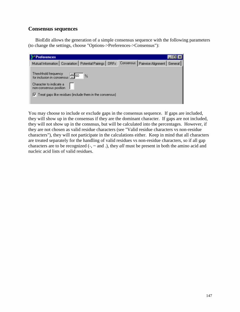
147
Consensus sequences
BioEdit allows the generation of a simple consensus sequence with the following parameters
(to change the settings, choose "Options->Preferences->Consensus"):
You may choose to include or exclude gaps in the consensus sequence. If gaps are included,
they will show up in the consensus if they are the dominant character. If gaps are not included,
they will not show up in the consnsus, but will be calculated into the percentages. However, if
they are not chosen as valid residue characters (see "Valid residue characters vs non-residue
characters"), they will not participate in the calculations either. Keep in mind that all characters
are treated separately for the handling of valid residues vs non-residue characters, so if all gap
characters are to be recognized (-, ~ and .), they all must be present in both the amino acid and
nucleic acid lists of valid residues.
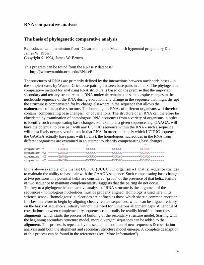
148
RNA comparative analysis
The basis of phylogenetic comparative analysis
Reproduced with permission from “Covariation”, the Macintosh hypercard program by Dr.
James W. Brown
Copyright © 1994, James W. Brown
This program can be found from the RNase P database:
http://jwbrown.mbio.ncsu.edu/RNaseP
The structures of RNAs are primarily defined by the interactions between nucleotide bases - in
the simplest case, by Watson-Crick base-pairing between base pairs in a helix. The phylogenetic
comparative method for analyzing RNA structure is based on the premise that the important
secondary and tertiary structure in an RNA molecule remains the same despite changes in the
nucleotide sequence of the RNA during evolution; any change in the sequence that might disrupt
the structure is compensated for by change elsewhere in the sequence that allows the
maintenance of the active structure. The homologous RNAs of different organisms will therefore
contain "compensating base changes", or covariations. The structure of an RNA can therefore be
elucidated by examination of homologous RNA sequences from a variety of organisms in order
to identify such compensating base changes. For example, a given sequence, e.g. GAAGA, will
have the potential to base pair with any UCUUC sequence within the RNA - such a sequence
will most likely occur several times in that RNA. In order to identify which UCUUC sequence
the GAAGA actually base pairs with (if any), the homologous nucleotides in the RNA from
different organisms are examined in an attempt to identify compensating base changes: * x x *
organism #1 -----GAAGA---------UCUUC--------UCUUC---------UCUUC-------
organism #2 -----GAUGA---------UCUUC--------UCUGC---------UCAUC-------
organism #2 -----GAUGA---------GCUUC--------UCUAC---------UCAUC-------
organism #2 -----GACGA---------UCUUC--------UCUGC---------UCGUC-------
In the above example, only the last UCUUC (UCUUC in organism #1, that is) sequence changes
to maintain the ability to base pair with the GAAGA sequence. Such compensating base changes
at two positions in a potential helix are considered "proof" of the presence of that helix. Failure
of two sequence to maintain complementarity suggests that the pairing do not occur.
The key to a phylogenetic comparative analysis of RNA structure is the alignment of the
sequences - homologous nucleotides must be properly aligned. Homology is used here in its
strictest sense - "homologous" nucleotides are defined as those which share a common ancestor.
It is best therefore to begin by aligning closely related sequences, which can be aligned reliably
on the basis of sequence similarity without the need for numerous alignment gaps. A handful of
covariations between complementary sequences can usually be readily identified from these
alignments, which starts the process of building of the secondary structure model. Starting with
the beginning secondary structure model, more divergent sequences can be added to the
alignment. This process is repeated by the sequential addition of new sequences & covariation
analysis until both the alignment and secondary structure model emerge. A complete description
of this process can be found in the references (see "More Information").

149
Once a complete secondary structure model is available, covariation analysis can be used to
identify interactions between nucleotides that are not in helices (higher-order structure),
non-canonical interactions, etc. Such interactions are identified because the associated
nucleotides will vary in concert (i.e. covary), even if the do not form a canonical base pair or are
part of a longer helix.
150
Using Masks
Masks are used to indicate a subsection of an alignment to be included in an analysis, at the
exclusion of everything else. For example, if you have an alignment of long RNA sequences and
you want to do a comparative analysis on only a small region to decipher a localized secondary
structure, you might want to exclude from the analysis the parts of the sequences that you do not
want data for. By specifying a mask prior to running covariation, potential pairings or mutual
information analyses, you tell the program to report data only for specified positions. Sometimes
one wishes to analyze an RNA secondary structure element in a structure for which a
standardized numbering system based on the structure from one organism exists (for example the
RNase P RNA from E. coli is often used to number nearly universal positions for all bacterial
RNase P RNAs). For this purpose, a sequence may be set as a numbering mask, and positions of
bases in a comparative analysis will be numbered to correspond to the numbering mask. Often
the numbering mask and sequence mask are the same.
Conventions used in BioEdit for masks:
For any mask, the three characters ‘-’, ‘~’ and ‘.’ (all gap indicators) designate that a position is
not to be included in an analysis.
Any other character specifies that the position be included.
For masks created in BioEdit, a ‘*’ generally indicates inclusion, a ‘-’ indicates exclusion.
A mask might look like this:
-----**********-----**********-----
This specifies that the first 5 are excluded, the next 10 included, etc.
A sequence and numbering mask may be used simultaneously in an analysis, but neither one is a
requirement. If the numbering is set to mask numbering in an analysis preferences set, then there
must be a numbering mask specified.
To set a sequence as a mask or numbering mask, choose the “Set as Sequence Mask” or “Set as
Numbering Mask” option under the “Sequence” menu.
To create a new mask, select the “Create New Mask” option under the “Sequence” menu. The
new mask will be created as a series of asterisks (e.g.
“***********************************************”)
To toggle mask positions on or off, select the region to be toggled with the mouse, then choose
“Toggle Mask” under the ”Sequence” menu.
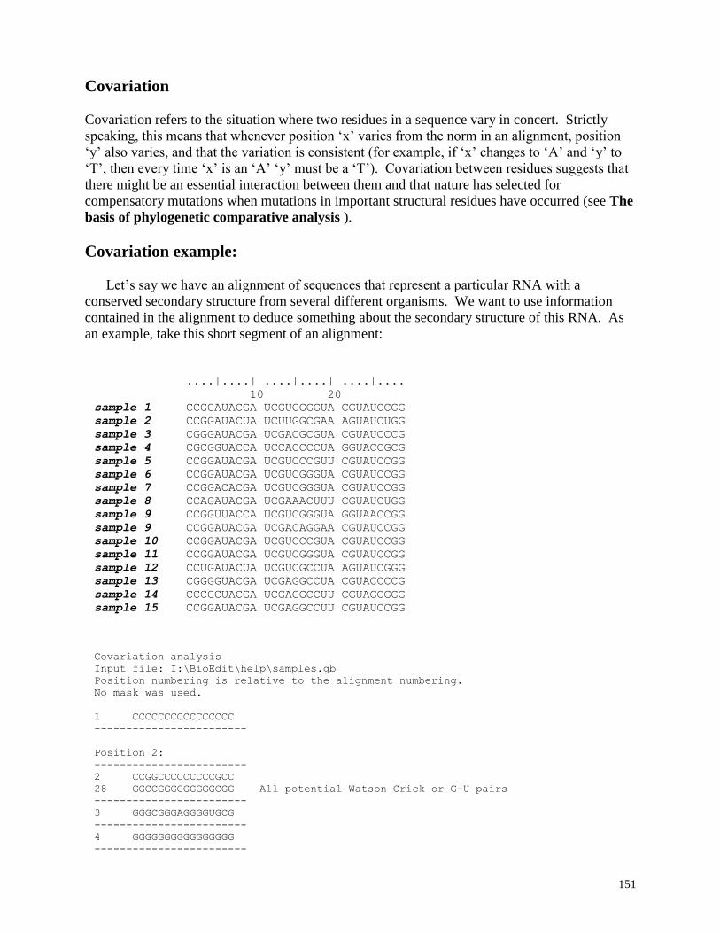
151
Covariation
Covariation refers to the situation where two residues in a sequence vary in concert. Strictly
speaking, this means that whenever position ‘x’ varies from the norm in an alignment, position
‘y’ also varies, and that the variation is consistent (for example, if ‘x’ changes to ‘A’ and ‘y’ to
‘T’, then every time ‘x’ is an ‘A’ ‘y’ must be a ‘T’). Covariation between residues suggests that
there might be an essential interaction between them and that nature has selected for
compensatory mutations when mutations in important structural residues have occurred (see The
basis of phylogenetic comparative analysis ).
Covariation example:
Let’s say we have an alignment of sequences that represent a particular RNA with a
conserved secondary structure from several different organisms. We want to use information
contained in the alignment to deduce something about the secondary structure of this RNA. As
an example, take this short segment of an alignment:
....|....| ....|....| ....|....
10 20
sample 1 CCGGAUACGA UCGUCGGGUA CGUAUCCGG
sample 2 CCGGAUACUA UCUUGGCGAA AGUAUCUGG
sample 3 CGGGAUACGA UCGACGCGUA CGUAUCCCG
sample 4 CGCGGUACCA UCCACCCCUA GGUACCGCG
sample 5 CCGGAUACGA UCGUCCCGUU CGUAUCCGG
sample 6 CCGGAUACGA UCGUCGGGUA CGUAUCCGG
sample 7 CCGGACACGA UCGUCGGGUA CGUAUCCGG
sample 8 CCAGAUACGA UCGAAACUUU CGUAUCUGG
sample 9 CCGGUUACCA UCGUCGGGUA GGUAACCGG
sample 9 CCGGAUACGA UCGACAGGAA CGUAUCCGG
sample 10 CCGGAUACGA UCGUCCCGUA CGUAUCCGG
sample 11 CCGGAUACGA UCGUCGGGUA CGUAUCCGG
sample 12 CCUGAUACUA UCGUCGCCUA AGUAUCGGG
sample 13 CGGGGUACGA UCGAGGCCUA CGUACCCCG
sample 14 CCCGCUACGA UCGAGGCCUU CGUAGCGGG
sample 15 CCGGAUACGA UCGAGGCCUU CGUAUCCGG
Covariation analysis
Input file: I:\BioEdit\help\samples.gb
Position numbering is relative to the alignment numbering.
No mask was used.
1 CCCCCCCCCCCCCCCC
------------------------
Position 2:
------------------------
2 CCGGCCCCCCCCCGCC
28 GGCCGGGGGGGGGCGG All potential Watson Crick or G-U pairs
------------------------
3 GGGCGGGAGGGGUGCG
------------------------
4 GGGGGGGGGGGGGGGG
------------------------
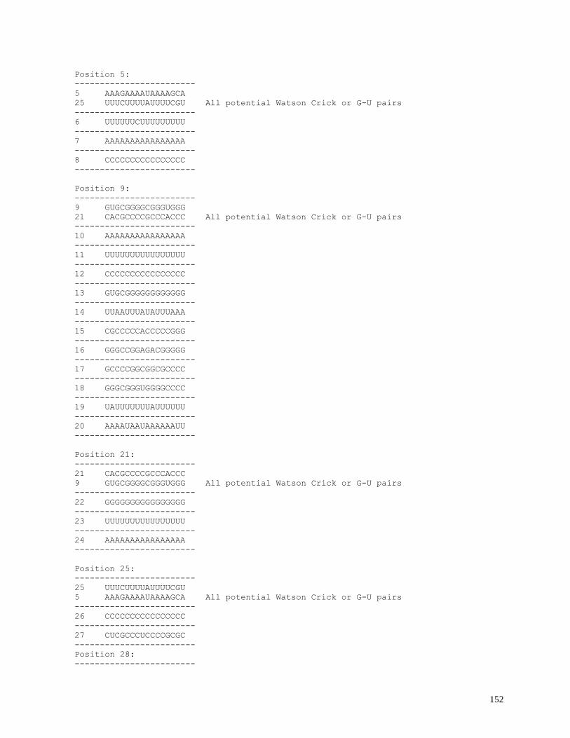
152
Position 5:
------------------------
5 AAAGAAAAUAAAAGCA
25 UUUCUUUUAUUUUCGU All potential Watson Crick or G-U pairs
------------------------
6 UUUUUUCUUUUUUUUU
------------------------
7 AAAAAAAAAAAAAAAA
------------------------
8 CCCCCCCCCCCCCCCC
------------------------
Position 9:
------------------------
9 GUGCGGGGCGGGUGGG
21 CACGCCCCGCCCACCC All potential Watson Crick or G-U pairs
------------------------
10 AAAAAAAAAAAAAAAA
------------------------
11 UUUUUUUUUUUUUUUU
------------------------
12 CCCCCCCCCCCCCCCC
------------------------
13 GUGCGGGGGGGGGGGG
------------------------
14 UUAAUUUAUAUUUAAA
------------------------
15 CGCCCCCACCCCCGGG
------------------------
16 GGGCCGGAGACGGGGG
------------------------
17 GCCCCGGCGGCGCCCC
------------------------
18 GGGCGGGUGGGGCCCC
------------------------
19 UAUUUUUUUAUUUUUU
------------------------
20 AAAAUAAUAAAAAAUU
------------------------
Position 21:
------------------------
21 CACGCCCCGCCCACCC
9 GUGCGGGGCGGGUGGG All potential Watson Crick or G-U pairs
------------------------
22 GGGGGGGGGGGGGGGG
------------------------
23 UUUUUUUUUUUUUUUU
------------------------
24 AAAAAAAAAAAAAAAA
------------------------
Position 25:
------------------------
25 UUUCUUUUAUUUUCGU
5 AAAGAAAAUAAAAGCA All potential Watson Crick or G-U pairs
------------------------
26 CCCCCCCCCCCCCCCC
------------------------
27 CUCGCCCUCCCCGCGC
------------------------
Position 28:
------------------------
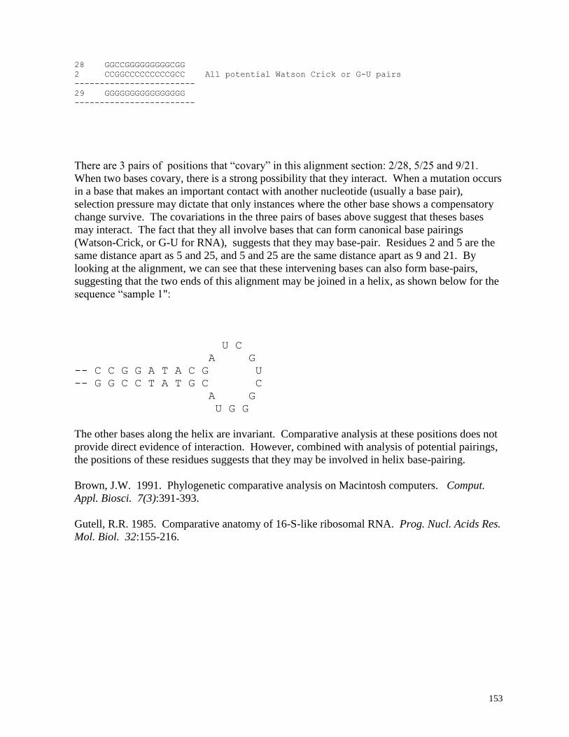
153
28 GGCCGGGGGGGGGCGG
2 CCGGCCCCCCCCCGCC All potential Watson Crick or G-U pairs
------------------------
29 GGGGGGGGGGGGGGGG
------------------------
There are 3 pairs of positions that “covary” in this alignment section: 2/28, 5/25 and 9/21.
When two bases covary, there is a strong possibility that they interact. When a mutation occurs
in a base that makes an important contact with another nucleotide (usually a base pair),
selection pressure may dictate that only instances where the other base shows a compensatory
change survive. The covariations in the three pairs of bases above suggest that theses bases
may interact. The fact that they all involve bases that can form canonical base pairings
(Watson-Crick, or G-U for RNA), suggests that they may base-pair. Residues 2 and 5 are the
same distance apart as 5 and 25, and 5 and 25 are the same distance apart as 9 and 21. By
looking at the alignment, we can see that these intervening bases can also form base-pairs,
suggesting that the two ends of this alignment may be joined in a helix, as shown below for the
sequence “sample 1":
U C
A G
-- C C G G A T A C G U
-- G G C C T A T G C C
A G
U G G
The other bases along the helix are invariant. Comparative analysis at these positions does not
provide direct evidence of interaction. However, combined with analysis of potential pairings,
the positions of these residues suggests that they may be involved in helix base-pairing.
Brown, J.W. 1991. Phylogenetic comparative analysis on Macintosh computers. Comput.
Appl. Biosci. 7(3):391-393.
Gutell, R.R. 1985. Comparative anatomy of 16-S-like ribosomal RNA. Prog. Nucl. Acids Res.
Mol. Biol. 32:155-216.
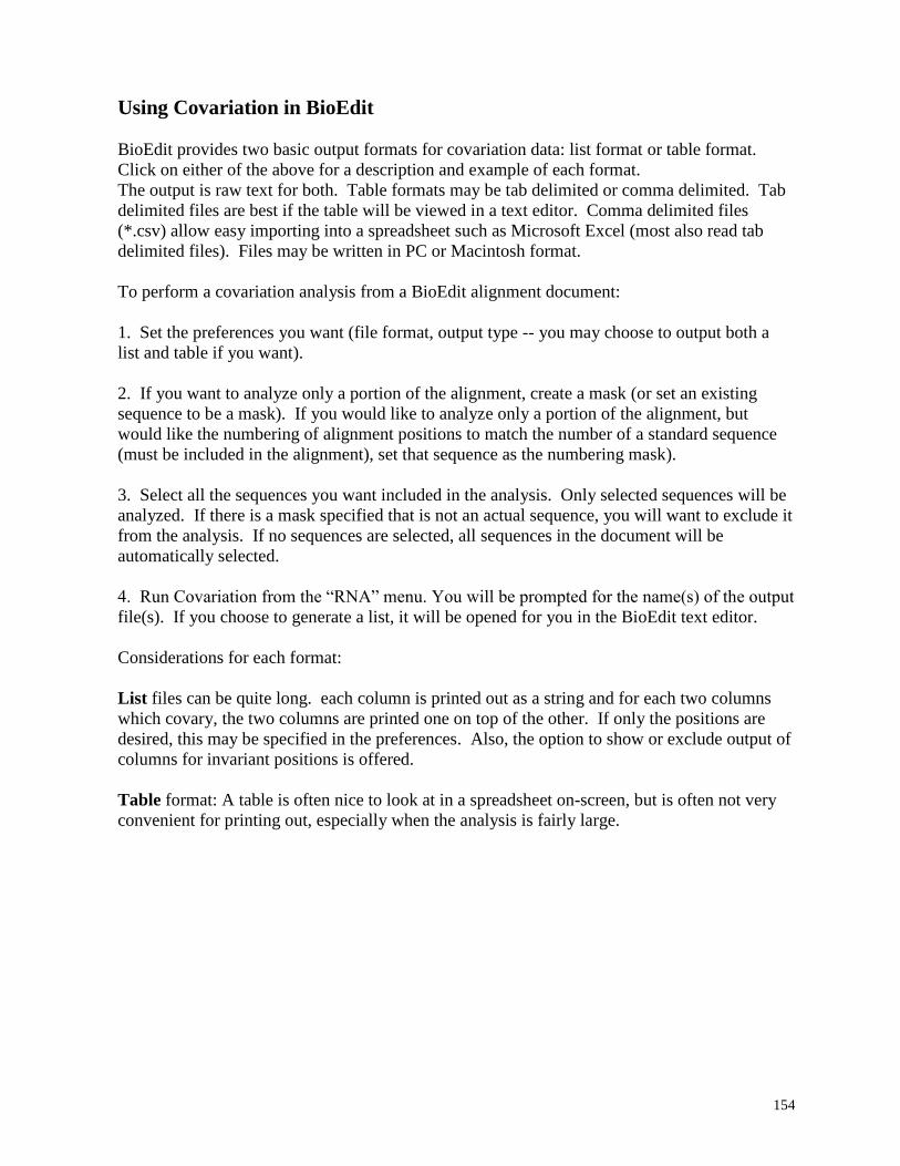
154
Using Covariation in BioEdit
BioEdit provides two basic output formats for covariation data: list format or table format.
Click on either of the above for a description and example of each format.
The output is raw text for both. Table formats may be tab delimited or comma delimited. Tab
delimited files are best if the table will be viewed in a text editor. Comma delimited files
(*.csv) allow easy importing into a spreadsheet such as Microsoft Excel (most also read tab
delimited files). Files may be written in PC or Macintosh format.
To perform a covariation analysis from a BioEdit alignment document:
1. Set the preferences you want (file format, output type -- you may choose to output both a
list and table if you want).
2. If you want to analyze only a portion of the alignment, create a mask (or set an existing
sequence to be a mask). If you would like to analyze only a portion of the alignment, but
would like the numbering of alignment positions to match the number of a standard sequence
(must be included in the alignment), set that sequence as the numbering mask).
3. Select all the sequences you want included in the analysis. Only selected sequences will be
analyzed. If there is a mask specified that is not an actual sequence, you will want to exclude it
from the analysis. If no sequences are selected, all sequences in the document will be
automatically selected.
4. Run Covariation from the “RNA” menu. You will be prompted for the name(s) of the output
file(s). If you choose to generate a list, it will be opened for you in the BioEdit text editor.
Considerations for each format:
List files can be quite long. each column is printed out as a string and for each two columns
which covary, the two columns are printed one on top of the other. If only the positions are
desired, this may be specified in the preferences. Also, the option to show or exclude output of
columns for invariant positions is offered.
Table format: A table is often nice to look at in a spreadsheet on-screen, but is often not very
convenient for printing out, especially when the analysis is fairly large.

155
Table output
Covariation tables are formatted as a 2-dimensional matrix of alignment positions (each
position compared to every other position). When two positions covary, a ‘5' is placed at the
matrix intersection of the two positions. If both of the positions are invariant, a ‘1' is placed in
that position. When they are not both invariant and do not covary, a 0 is placed at their
intersection.
As an example, take the following short alignment:
....|....| ....|....| ....|....
10 20
sample 1 CCGGAUACGA UCGUCGGGUA CGUAUCCGG
sample 2 CCGGAUACUA UCUUGGCGAA AGUAUCCGG
sample 3 CGGGAUACGA UCGACGCGUA CGUAUCCCG
sample 4 CGGGGUACCA UCCACCCCUA GGUACCCCG
sample 5 CCGGAUACGA UCGUCCCGUU CGUAUCCGG
sample 6 CCGGAUACGA UCGUCGGGUA CGUAUCCGG
sample 7 CCGGAUACGA UCGUCGGGUA CGUAUCCGG
sample 8 CCGGAUACGA UCGAAACUUU CGUAUCCGG
sample 9 CCGGUUACCA UCGUCGGGUA GGUAACCGG
sample 9 CCGGAUACGA UCGACAGGAA CGUAUCCGG
sample 10 CCGGAUACGA UCGUCCCGUA CGUAUCCGG
sample 11 CCGGAUACGA UCGUCGGGUA CGUAUCCGG
sample 12 CCGGAUACUA UCGUCGCCUA AGUAUCCGG
sample 13 CGGGGUACGA UCGAGGCCUA CGUACCCCG
sample 14 CCGGCUACGA UCGAGGCCUU CGUAGCCGG
sample 15 CCGGAUACGA UCGAGGCCUU CGUAUCCGG
Table output of covariation data would look like this (larger tables will appear wrapped in a word
processor, but may be viewed unwrapped in an editor such as WordPad):
Covariation analysis
Input file: D:\BioEdit\help\samples.gb
Matrix Output
5 = Covariation, 1 = Invariant
Position numbering is relative to the alignment numbering.
No mask was used.
1 2 3 4 5 6 7 8 9 10 11 12 13 14 15 16 17 18 19 20 21 22 23 24 25 26 27 28 29
1 0 0 1 1 0 1 1 1 0 1 1 1 0 0 0 0 0 0 0 0 0 1 1 1 0 1 1 0 1
2 0 0 0 0 0 0 0 0 0 0 0 0 0 0 0 0 0 0 0 0 0 0 0 0 0 0 0 5 0
3 1 0 0 1 0 1 1 1 0 1 1 1 0 0 0 0 0 0 0 0 0 1 1 1 0 1 1 0 1
4 1 0 1 0 0 1 1 1 0 1 1 1 0 0 0 0 0 0 0 0 0 1 1 1 0 1 1 0 1
5 0 0 0 0 0 0 0 0 0 0 0 0 0 0 0 0 0 0 0 0 0 0 0 0 5 0 0 0 0
6 1 0 1 1 0 0 1 1 0 1 1 1 0 0 0 0 0 0 0 0 0 1 1 1 0 1 1 0 1
7 1 0 1 1 0 1 0 1 0 1 1 1 0 0 0 0 0 0 0 0 0 1 1 1 0 1 1 0 1
8 1 0 1 1 0 1 1 0 0 1 1 1 0 0 0 0 0 0 0 0 0 1 1 1 0 1 1 0 1
9 0 0 0 0 0 0 0 0 0 0 0 0 0 0 0 0 0 0 0 0 5 0 0 0 0 0 0 0 0
10 1 0 1 1 0 1 1 1 0 0 1 1 0 0 0 0 0 0 0 0 0 1 1 1 0 1 1 0 1
11 1 0 1 1 0 1 1 1 0 1 0 1 0 0 0 0 0 0 0 0 0 1 1 1 0 1 1 0 1
12 1 0 1 1 0 1 1 1 0 1 1 0 0 0 0 0 0 0 0 0 0 1 1 1 0 1 1 0 1
13 0 0 0 0 0 0 0 0 0 0 0 0 0 0 0 0 0 0 0 0 0 0 0 0 0 0 0 0 0
14 0 0 0 0 0 0 0 0 0 0 0 0 0 0 0 0 0 0 0 0 0 0 0 0 0 0 0 0 0
15 0 0 0 0 0 0 0 0 0 0 0 0 0 0 0 0 0 0 0 0 0 0 0 0 0 0 0 0 0
16 0 0 0 0 0 0 0 0 0 0 0 0 0 0 0 0 0 0 0 0 0 0 0 0 0 0 0 0 0
17 0 0 0 0 0 0 0 0 0 0 0 0 0 0 0 0 0 0 0 0 0 0 0 0 0 0 0 0 0
18 0 0 0 0 0 0 0 0 0 0 0 0 0 0 0 0 0 0 0 0 0 0 0 0 0 0 0 0 0
19 0 0 0 0 0 0 0 0 0 0 0 0 0 0 0 0 0 0 0 0 0 0 0 0 0 0 0 0 0
20 0 0 0 0 0 0 0 0 0 0 0 0 0 0 0 0 0 0 0 0 0 0 0 0 0 0 0 0 0
21 0 0 0 0 0 0 0 0 5 0 0 0 0 0 0 0 0 0 0 0 0 0 0 0 0 0 0 0 0
22 1 0 1 1 0 1 1 1 0 1 1 1 0 0 0 0 0 0 0 0 0 0 1 1 0 1 1 0 1
23 1 0 1 1 0 1 1 1 0 1 1 1 0 0 0 0 0 0 0 0 0 1 0 1 0 1 1 0 1
24 1 0 1 1 0 1 1 1 0 1 1 1 0 0 0 0 0 0 0 0 0 1 1 0 0 1 1 0 1
25 0 0 0 0 5 0 0 0 0 0 0 0 0 0 0 0 0 0 0 0 0 0 0 0 0 0 0 0 0
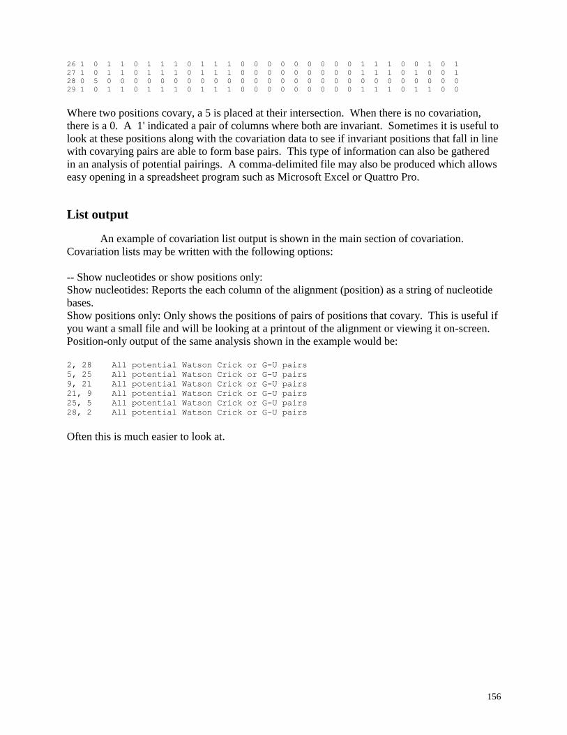
156
26 1 0 1 1 0 1 1 1 0 1 1 1 0 0 0 0 0 0 0 0 0 1 1 1 0 0 1 0 1
27 1 0 1 1 0 1 1 1 0 1 1 1 0 0 0 0 0 0 0 0 0 1 1 1 0 1 0 0 1
28 0 5 0 0 0 0 0 0 0 0 0 0 0 0 0 0 0 0 0 0 0 0 0 0 0 0 0 0 0
29 1 0 1 1 0 1 1 1 0 1 1 1 0 0 0 0 0 0 0 0 0 1 1 1 0 1 1 0 0
Where two positions covary, a 5 is placed at their intersection. When there is no covariation,
there is a 0. A 1' indicated a pair of columns where both are invariant. Sometimes it is useful to
look at these positions along with the covariation data to see if invariant positions that fall in line
with covarying pairs are able to form base pairs. This type of information can also be gathered
in an analysis of potential pairings. A comma-delimited file may also be produced which allows
easy opening in a spreadsheet program such as Microsoft Excel or Quattro Pro.
List output
An example of covariation list output is shown in the main section of covariation.
Covariation lists may be written with the following options:
-- Show nucleotides or show positions only:
Show nucleotides: Reports the each column of the alignment (position) as a string of nucleotide
bases.
Show positions only: Only shows the positions of pairs of positions that covary. This is useful if
you want a small file and will be looking at a printout of the alignment or viewing it on-screen.
Position-only output of the same analysis shown in the example would be:
2, 28 All potential Watson Crick or G-U pairs
5, 25 All potential Watson Crick or G-U pairs
9, 21 All potential Watson Crick or G-U pairs
21, 9 All potential Watson Crick or G-U pairs
25, 5 All potential Watson Crick or G-U pairs
28, 2 All potential Watson Crick or G-U pairs
Often this is much easier to look at.
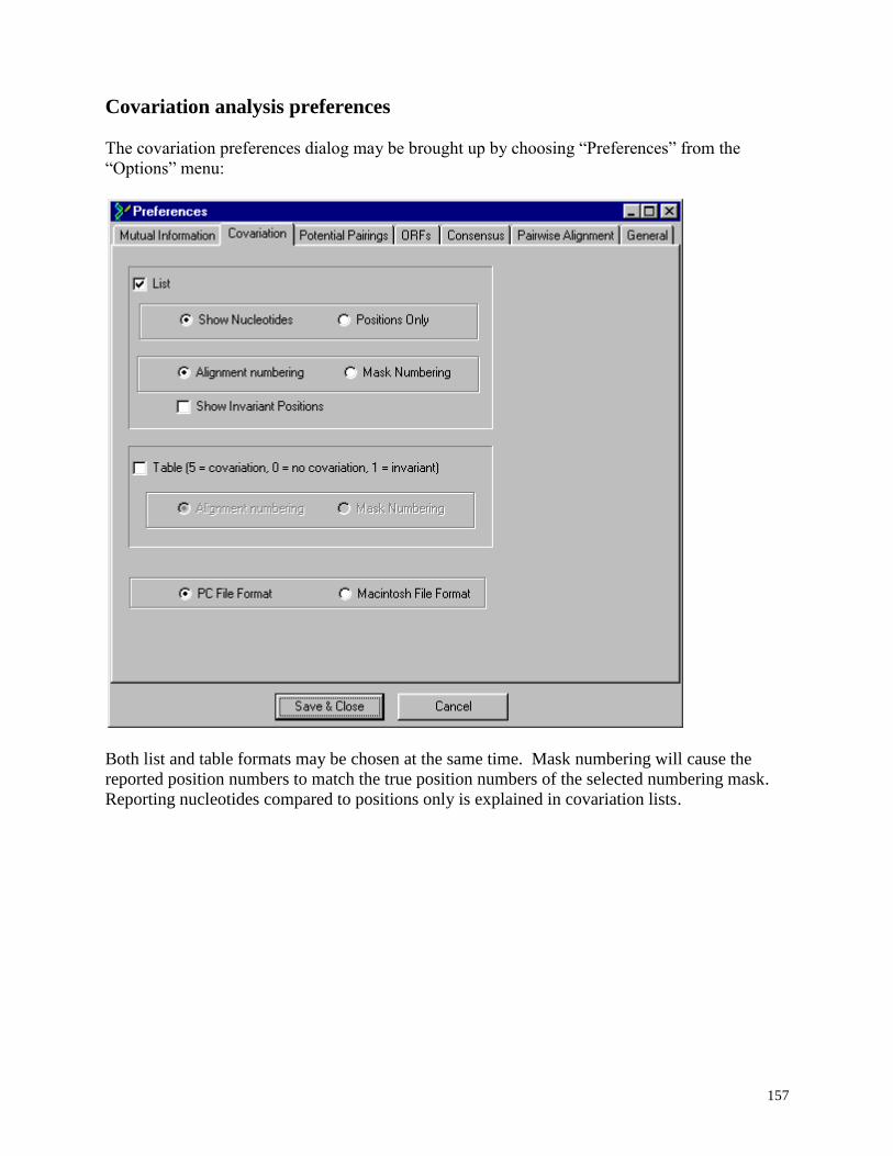
157
Covariation analysis preferences
The covariation preferences dialog may be brought up by choosing “Preferences” from the
“Options” menu:
Both list and table formats may be chosen at the same time. Mask numbering will cause the
reported position numbers to match the true position numbers of the selected numbering mask.
Reporting nucleotides compared to positions only is explained in covariation lists.
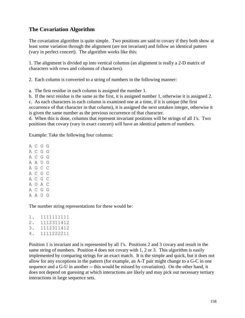
158
The Covariation Algorithm
The covariation algorithm is quite simple. Two positions are said to covary if they both show at
least some variation through the alignment (are not invariant) and follow an identical pattern
(vary in perfect concert). The algorithm works like this:
1. The alignment is divided up into vertical columns (an alignment is really a 2-D matrix of
characters with rows and columns of characters).
2. Each column is converted to a string of numbers in the following manner:
a. The first residue in each column is assigned the number 1.
b. If the next residue is the same as the first, it is assigned number 1, otherwise it is assigned 2.
c. As each characters in each column is examined one at a time, if it is unique (the first
occurrence of that character in that column), it is assigned the next untaken integer, otherwise it
is given the same number as the previous occurrence of that character.
d. When this is done, columns that represent invariant positions will be strings of all 1's. Two
positions that covary (vary in exact concert) will have an identical pattern of numbers.
Example: Take the following four columns:
A C G G
A C G G
A C G G
A A U G
A G C C
A C G C
A C G C
A U A C
A C G G
A A U G
The number string representations for these would be:
1. 1111111111
2. 1112311412
3. 1112311412
4. 1111222211
Position 1 is invariant and is represented by all 1's. Positions 2 and 3 covary and result in the
same string of numbers. Position 4 does not covary with 1, 2 or 3. This algorithm is easily
implemented by comparing strings for an exact match. It is the simple and quick, but it does not
allow for any exceptions in the pattern (for example, an A-T pair might change to a G-C in one
sequence and a G-U in another -- this would be missed by covariation). On the other hand, it
does not depend on guessing at which interactions are likely and may pick out necessary tertiary
interactions in large sequence sets.

159
Brown, J.W. 1991. Phylogenetic comparative analysis on Macintosh computers. Comput.
Appl. Biosci. 7(3):391-393.
Gutell, R.R. 1985. Comparative anatomy of 16-S-like ribosomal RNA. Prog. Nucl. Acids Res.
Mol. Biol. 32:155-216.
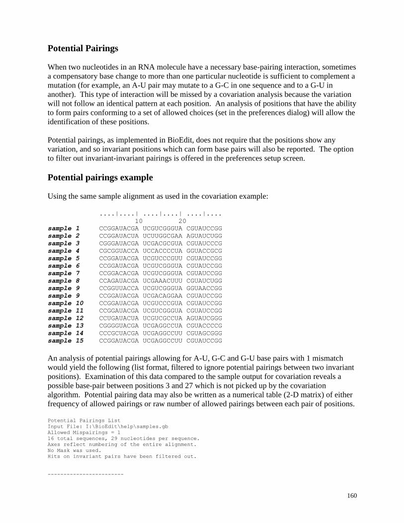
160
Potential Pairings
When two nucleotides in an RNA molecule have a necessary base-pairing interaction, sometimes
a compensatory base change to more than one particular nucleotide is sufficient to complement a
mutation (for example, an A-U pair may mutate to a G-C in one sequence and to a G-U in
another). This type of interaction will be missed by a covariation analysis because the variation
will not follow an identical pattern at each position. An analysis of positions that have the ability
to form pairs conforming to a set of allowed choices (set in the preferences dialog) will allow the
identification of these positions.
Potential pairings, as implemented in BioEdit, does not require that the positions show any
variation, and so invariant positions which can form base pairs will also be reported. The option
to filter out invariant-invariant pairings is offered in the preferences setup screen.
Potential pairings example
Using the same sample alignment as used in the covariation example:
....|....| ....|....| ....|....
10 20
sample 1 CCGGAUACGA UCGUCGGGUA CGUAUCCGG
sample 2 CCGGAUACUA UCUUGGCGAA AGUAUCUGG
sample 3 CGGGAUACGA UCGACGCGUA CGUAUCCCG
sample 4 CGCGGUACCA UCCACCCCUA GGUACCGCG
sample 5 CCGGAUACGA UCGUCCCGUU CGUAUCCGG
sample 6 CCGGAUACGA UCGUCGGGUA CGUAUCCGG
sample 7 CCGGACACGA UCGUCGGGUA CGUAUCCGG
sample 8 CCAGAUACGA UCGAAACUUU CGUAUCUGG
sample 9 CCGGUUACCA UCGUCGGGUA GGUAACCGG
sample 9 CCGGAUACGA UCGACAGGAA CGUAUCCGG
sample 10 CCGGAUACGA UCGUCCCGUA CGUAUCCGG
sample 11 CCGGAUACGA UCGUCGGGUA CGUAUCCGG
sample 12 CCUGAUACUA UCGUCGCCUA AGUAUCGGG
sample 13 CGGGGUACGA UCGAGGCCUA CGUACCCCG
sample 14 CCCGCUACGA UCGAGGCCUU CGUAGCGGG
sample 15 CCGGAUACGA UCGAGGCCUU CGUAUCCGG
An analysis of potential pairings allowing for A-U, G-C and G-U base pairs with 1 mismatch
would yield the following (list format, filtered to ignore potential pairings between two invariant
positions). Examination of this data compared to the sample output for covariation reveals a
possible base-pair between positions 3 and 27 which is not picked up by the covariation
algorithm. Potential pairing data may also be written as a numerical table (2-D matrix) of either
frequency of allowed pairings or raw number of allowed pairings between each pair of positions.
Potential Pairings List
Input File: I:\BioEdit\help\samples.gb
Allowed Mispairings = 1
16 total sequences, 29 nucleotides per sequence.
Axes reflect numbering of the entire alignment.
No Mask was used.
Hits on invariant pairs have been filtered out.
------------------------
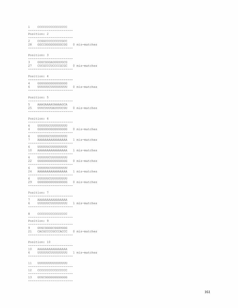
161
1 CCCCCCCCCCCCCCCC
------------------------
Position: 2
------------------------
2 CCGGCCCCCCCCCGCC
28 GGCCGGGGGGGGGCGG 0 mis-matches
------------------------
Position: 3
------------------------
3 GGGCGGGAGGGGUGCG
27 CUCGCCCUCCCCGCGC 0 mis-matches
------------------------
Position: 4
------------------------
4 GGGGGGGGGGGGGGGG
6 UUUUUUCUUUUUUUUU 0 mis-matches
------------------------
Position: 5
------------------------
5 AAAGAAAAUAAAAGCA
25 UUUCUUUUAUUUUCGU 0 mis-matches
------------------------
Position: 6
------------------------
6 UUUUUUCUUUUUUUUU
4 GGGGGGGGGGGGGGGG 0 mis-matches
------------------------
6 UUUUUUCUUUUUUUUU
7 AAAAAAAAAAAAAAAA 1 mis-matches
------------------------
6 UUUUUUCUUUUUUUUU
10 AAAAAAAAAAAAAAAA 1 mis-matches
------------------------
6 UUUUUUCUUUUUUUUU
22 GGGGGGGGGGGGGGGG 0 mis-matches
------------------------
6 UUUUUUCUUUUUUUUU
24 AAAAAAAAAAAAAAAA 1 mis-matches
------------------------
6 UUUUUUCUUUUUUUUU
29 GGGGGGGGGGGGGGGG 0 mis-matches
------------------------
Position: 7
------------------------
7 AAAAAAAAAAAAAAAA
6 UUUUUUCUUUUUUUUU 1 mis-matches
------------------------
8 CCCCCCCCCCCCCCCC
------------------------
Position: 9
------------------------
9 GUGCGGGGCGGGUGGG
21 CACGCCCCGCCCACCC 0 mis-matches
------------------------
Position: 10
------------------------
10 AAAAAAAAAAAAAAAA
6 UUUUUUCUUUUUUUUU 1 mis-matches
------------------------
11 UUUUUUUUUUUUUUUU
------------------------
12 CCCCCCCCCCCCCCCC
------------------------
13 GUGCGGGGGGGGGGGG
------------------------
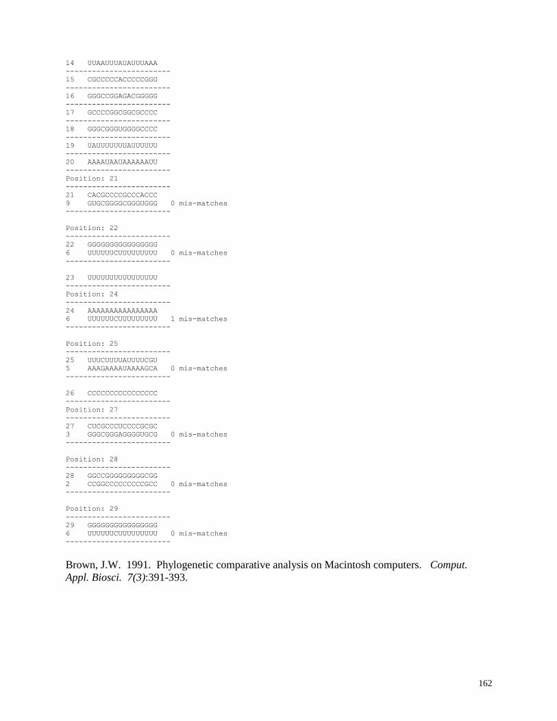
162
14 UUAAUUUAUAUUUAAA
------------------------
15 CGCCCCCACCCCCGGG
------------------------
16 GGGCCGGAGACGGGGG
------------------------
17 GCCCCGGCGGCGCCCC
------------------------
18 GGGCGGGUGGGGCCCC
------------------------
19 UAUUUUUUUAUUUUUU
------------------------
20 AAAAUAAUAAAAAAUU
------------------------
Position: 21
------------------------
21 CACGCCCCGCCCACCC
9 GUGCGGGGCGGGUGGG 0 mis-matches
------------------------
Position: 22
------------------------
22 GGGGGGGGGGGGGGGG
6 UUUUUUCUUUUUUUUU 0 mis-matches
------------------------
23 UUUUUUUUUUUUUUUU
------------------------
Position: 24
------------------------
24 AAAAAAAAAAAAAAAA
6 UUUUUUCUUUUUUUUU 1 mis-matches
------------------------
Position: 25
------------------------
25 UUUCUUUUAUUUUCGU
5 AAAGAAAAUAAAAGCA 0 mis-matches
------------------------
26 CCCCCCCCCCCCCCCC
------------------------
Position: 27
------------------------
27 CUCGCCCUCCCCGCGC
3 GGGCGGGAGGGGUGCG 0 mis-matches
------------------------
Position: 28
------------------------
28 GGCCGGGGGGGGGCGG
2 CCGGCCCCCCCCCGCC 0 mis-matches
------------------------
Position: 29
------------------------
29 GGGGGGGGGGGGGGGG
6 UUUUUUCUUUUUUUUU 0 mis-matches
------------------------
Brown, J.W. 1991. Phylogenetic comparative analysis on Macintosh computers. Comput.
Appl. Biosci. 7(3):391-393.
163
Using Potential Pairings in BioEdit
BioEdit provides two basic output formats for potential pairings data: lists or table format.
Click on either of the above for a description and example of each format.
The output is raw text for both. Table formats may be tab delimited or comma delimited. Tab
delimited files are best if the table will be viewed in a text editor. Comma delimited files (*.csv)
allow easy importing into a spreadsheet such as Microsoft Excel (most also read tab delimited
files). Files may be written in PC or Macintosh format.
To perform a potential pairings analysis from a BioEdit alignment document:
1. Set the preferences you want (file format, output type -- you may choose to output both a list
and table if you want).
2. Before staring, you will also want to decide which pairings are to be allowed. By default,
allowed pairings are initially set to A-T, C-G and G-U, but whenever preferences are saved from
the preferences dialog, these become the new defaults.
3. If you want to analyze only a portion of the alignment, create a mask (or set an existing
sequence to be a mask). If you would like to analyze only a portion of the alignment, but would
like the numbering of alignment positions to match the number of a standard sequence (must be
included in the alignment), set that sequence as the numbering mask).
4. Select all the sequences you want included in the analysis. Only selected sequences will be
analyzed. If there is a mask specified that is not an actual sequence, you will want to exclude it
from the analysis. If no sequences are selected, all sequences in the document will be
automatically selected.
5. Run “Potential Pairings” from the “RNA” menu of an open alignment document. You will be
prompted for the name(s) of the output file(s). If you choose to generate a list, it will be opened
for you in the BioEdit text editor.
Considerations for each format:
List files can be quite long. Invariant positions are shown and can often produce many
redundant matches that most likely don’t mean anything. For this reason, pairings between two
invariant positions may be filtered out.
Table format: A table is often nice to look at in a spreadsheet on-screen, but is often not very
convenient for printing out, especially when the analysis is fairly large.
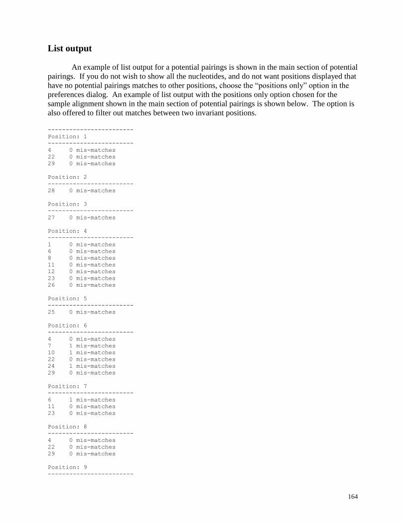
164
List output
An example of list output for a potential pairings is shown in the main section of potential
pairings. If you do not wish to show all the nucleotides, and do not want positions displayed that
have no potential pairings matches to other positions, choose the “positions only” option in the
preferences dialog. An example of list output with the positions only option chosen for the
sample alignment shown in the main section of potential pairings is shown below. The option is
also offered to filter out matches between two invariant positions.
------------------------
Position: 1
------------------------
4 0 mis-matches
22 0 mis-matches
29 0 mis-matches
Position: 2
------------------------
28 0 mis-matches
Position: 3
------------------------
27 0 mis-matches
Position: 4
------------------------
1 0 mis-matches
6 0 mis-matches
8 0 mis-matches
11 0 mis-matches
12 0 mis-matches
23 0 mis-matches
26 0 mis-matches
Position: 5
------------------------
25 0 mis-matches
Position: 6
------------------------
4 0 mis-matches
7 1 mis-matches
10 1 mis-matches
22 0 mis-matches
24 1 mis-matches
29 0 mis-matches
Position: 7
------------------------
6 1 mis-matches
11 0 mis-matches
23 0 mis-matches
Position: 8
------------------------
4 0 mis-matches
22 0 mis-matches
29 0 mis-matches
Position: 9
------------------------
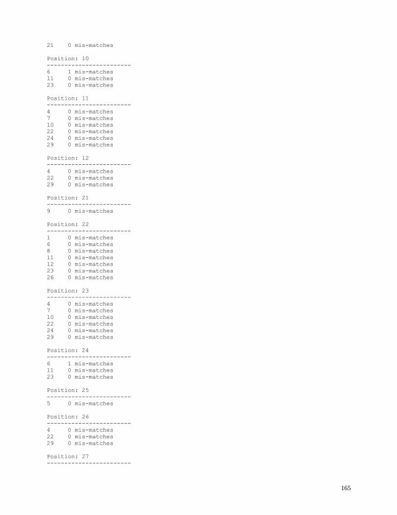
165
21 0 mis-matches
Position: 10
------------------------
6 1 mis-matches
11 0 mis-matches
23 0 mis-matches
Position: 11
------------------------
4 0 mis-matches
7 0 mis-matches
10 0 mis-matches
22 0 mis-matches
24 0 mis-matches
29 0 mis-matches
Position: 12
------------------------
4 0 mis-matches
22 0 mis-matches
29 0 mis-matches
Position: 21
------------------------
9 0 mis-matches
Position: 22
------------------------
1 0 mis-matches
6 0 mis-matches
8 0 mis-matches
11 0 mis-matches
12 0 mis-matches
23 0 mis-matches
26 0 mis-matches
Position: 23
------------------------
4 0 mis-matches
7 0 mis-matches
10 0 mis-matches
22 0 mis-matches
24 0 mis-matches
29 0 mis-matches
Position: 24
------------------------
6 1 mis-matches
11 0 mis-matches
23 0 mis-matches
Position: 25
------------------------
5 0 mis-matches
Position: 26
------------------------
4 0 mis-matches
22 0 mis-matches
29 0 mis-matches
Position: 27
------------------------
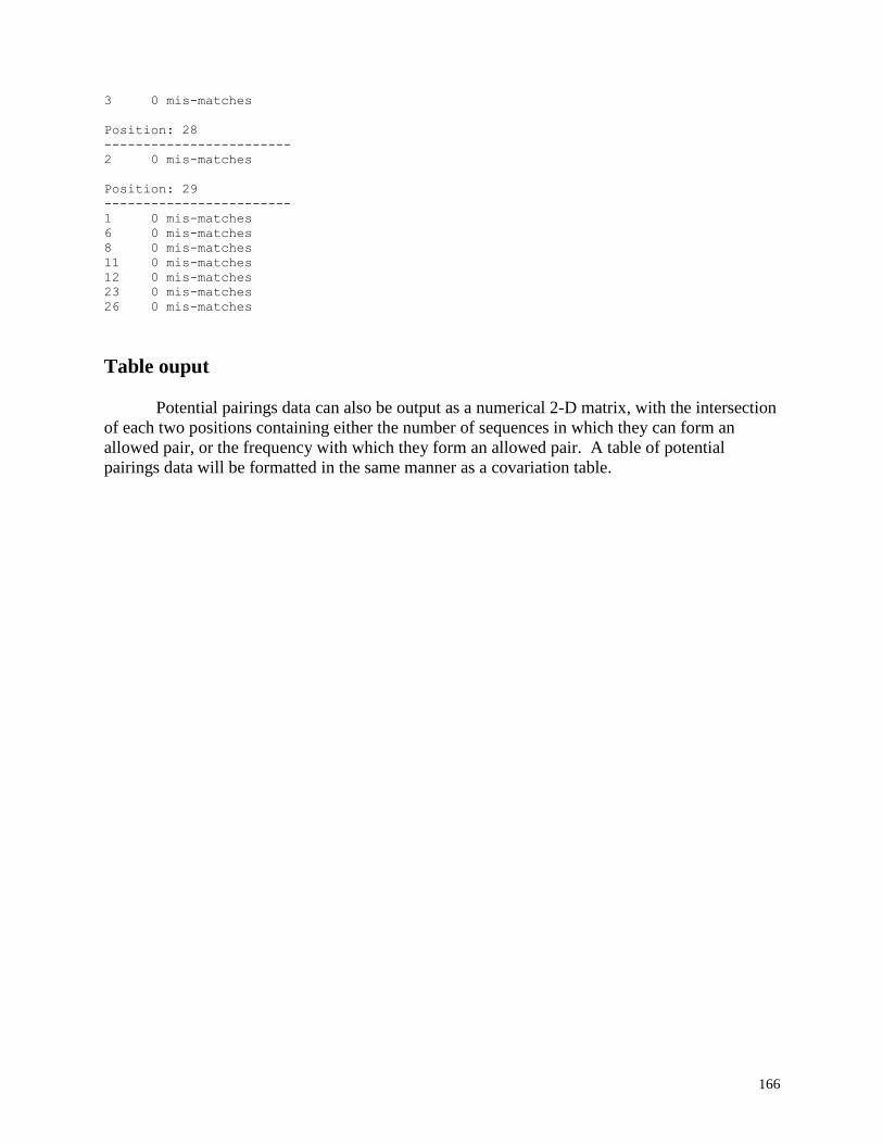
166
3 0 mis-matches
Position: 28
------------------------
2 0 mis-matches
Position: 29
------------------------
1 0 mis-matches
6 0 mis-matches
8 0 mis-matches
11 0 mis-matches
12 0 mis-matches
23 0 mis-matches
26 0 mis-matches
Table ouput
Potential pairings data can also be output as a numerical 2-D matrix, with the intersection
of each two positions containing either the number of sequences in which they can form an
allowed pair, or the frequency with which they form an allowed pair. A table of potential
pairings data will be formatted in the same manner as a covariation table.
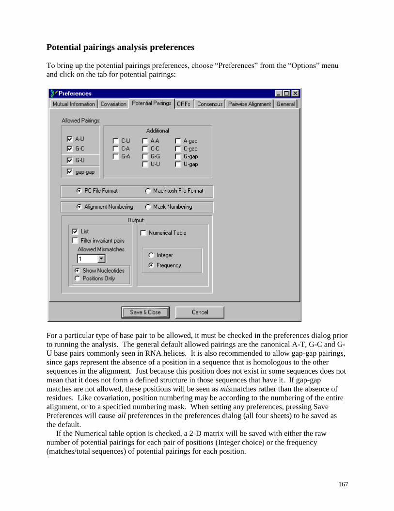
167
Potential pairings analysis preferences
To bring up the potential pairings preferences, choose “Preferences” from the “Options” menu
and click on the tab for potential pairings:
For a particular type of base pair to be allowed, it must be checked in the preferences dialog prior
to running the analysis. The general default allowed pairings are the canonical A-T, G-C and G-
U base pairs commonly seen in RNA helices. It is also recommended to allow gap-gap pairings,
since gaps represent the absence of a position in a sequence that is homologous to the other
sequences in the alignment. Just because this position does not exist in some sequences does not
mean that it does not form a defined structure in those sequences that have it. If gap-gap
matches are not allowed, these positions will be seen as mismatches rather than the absence of
residues. Like covariation, position numbering may be according to the numbering of the entire
alignment, or to a specified numbering mask. When setting any preferences, pressing Save
Preferences will cause all preferences in the preferences dialog (all four sheets) to be saved as
the default.
If the Numerical table option is checked, a 2-D matrix will be saved with either the raw
number of potential pairings for each pair of positions (Integer choice) or the frequency
(matches/total sequences) of potential pairings for each position.
168
The Potential Pairings Algorithm
The basic algorithm for potential pairings analysis is very straightforward and is
essentially a brute-force examination of every position compared to every other position in an
alignment against a set of allowed pairings.
Computationally, BioEdit approaches this numerically by assigning each nucleotide in each
sequence an integer value as follows:
A = 2
G = 3
C = 5
U = 9
GAP = 14
The sum of any two pairs of these numbers is unique (including each one paired to itself):
A+A = 4
A+C = 7
A+G = 5
A+U = 11
A+GAP =16
C+C = 10
C+G = 8
C+U = 14
C+GAP = 19
G+G = 6
G+U = 12
G+GAP = 17
U+U = 18
U+GAP = 23
GAP+GAP = 28
An array of 28 values which can take the value 1 or 0 is thus set up such that each of the
above sums represents the index to an array position holding a value which states that the pair is
allowed (1) or not allowed (0). As the residues are scanned for each pair of column positions in
the alignment, the value present at the array index of the sum of the two position residues for
each sequence is added to a total sum for that pair of positions (1 is added if the pair is a match,
otherwise 0 is added). If the total for a pair of positions is greater than or equal to the required
number (depends upon mismatches allowed), the potential pairing is reported in the output (for
table output, the total or total/number of sequences is reported for all positions).
169
Mutual Information Analysis
Before using mutual information as a structure probe, you probably want to read:
Gutell, R.R., A. Power, G.Z. Hertz, E.J. Putz and G.D. Stormo. 1992. Identifying constraints on
the higher-order structure of RNA: continued development and application of comparative
sequence analysis methods. Nucleic Acids Res. 20(21):5785-5795.
General Overview of Mutual Information
Mutual information, as applied to phylogenetic comparative analysis, is a measure of the
amount of information shared by two positions in a set of properly aligned sequences. This
measurement, symbolized as M(x,y) (the mutual information shared by positions x and y), gives
an idea of how strongly the identities of two positions are correlated, which is often a sign of
direct interaction such as base-pairing. Two other measurements that BioEdit will calculate, R1
and R2, give a measure of the contribution made by positions x and y to M(x,y). These
measurements are described at the end of mathematical overview of mutual information.
General Overview -- What is mutual information?
Mutual information analysis is an extension of the idea that information content may be
assessed as a general decrease in uncertainty about a particular situation. Given no prior
knowledge about a particular situation (such as the identity of a nucleotide in an RNA sequence),
uncertainty is at a maximum and one possesses no information about that situation. If the
identity of the nucleotide is discovered, uncertainty is removed and information about that
nucleotide is at a maximum. Now consider a large set of sequences, all of which contain a
homologous nucleotide at this position. Knowing the nucleotide’s identity in the first sequence
does not necessary offer much information about the same position in the next sequence or a
randomly chosen sequence. However, if the identity of this residue is known in many sequences,
and in nearly all of these sequences it is a particular base (say ‘C’), and is never a particular other
residue (say ‘G’), uncertainty drops way down about the possible identity of this base in an as yet
unexamined sequence. There is now considerable “information” accumulated about this base
which can be used to predict the probability of its identity being a particular base if a new
sequence is examined. This is the basis of the sequence logo (1) or the BioEdit implementation
of an entropy plot.
Mutual information extends this basic principal to examine the information content
shared between a pair of positions in an alignment. This is related to, and depends upon, the
information content of two individual positions, but refers specifically to the information that the
two positions possess together. More generally, it is a measure of the decrease in uncertainty
about the extent to which two things influence each other, or interact with each other. The use of
mutual information to probe RNA structure was developed by Robin Gutell (2). This measure is
ideally suited to phylogenetic comparative analysis because a high degree of mutual influence
between two positions may be a strong indication that these two residues directly interact.
As an example, examine the following small piece of an alignment:
1 2 3 4
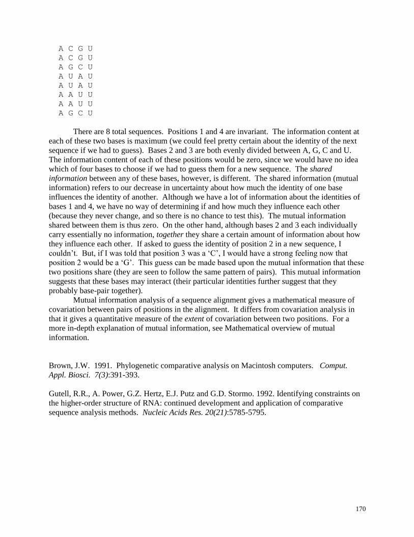
170
A C G U
A C G U
A G C U
A U A U
A U A U
A A U U
A A U U
A G C U
There are 8 total sequences. Positions 1 and 4 are invariant. The information content at
each of these two bases is maximum (we could feel pretty certain about the identity of the next
sequence if we had to guess). Bases 2 and 3 are both evenly divided between A, G, C and U.
The information content of each of these positions would be zero, since we would have no idea
which of four bases to choose if we had to guess them for a new sequence. The shared
information between any of these bases, however, is different. The shared information (mutual
information) refers to our decrease in uncertainty about how much the identity of one base
influences the identity of another. Although we have a lot of information about the identities of
bases 1 and 4, we have no way of determining if and how much they influence each other
(because they never change, and so there is no chance to test this). The mutual information
shared between them is thus zero. On the other hand, although bases 2 and 3 each individually
carry essentially no information, together they share a certain amount of information about how
they influence each other. If asked to guess the identity of position 2 in a new sequence, I
couldn’t. But, if I was told that position 3 was a ‘C’, I would have a strong feeling now that
position 2 would be a ‘G’. This guess can be made based upon the mutual information that these
two positions share (they are seen to follow the same pattern of pairs). This mutual information
suggests that these bases may interact (their particular identities further suggest that they
probably base-pair together).
Mutual information analysis of a sequence alignment gives a mathematical measure of
covariation between pairs of positions in the alignment. It differs from covariation analysis in
that it gives a quantitative measure of the extent of covariation between two positions. For a
more in-depth explanation of mutual information, see Mathematical overview of mutual
information.
Brown, J.W. 1991. Phylogenetic comparative analysis on Macintosh computers. Comput.
Appl. Biosci. 7(3):391-393.
Gutell, R.R., A. Power, G.Z. Hertz, E.J. Putz and G.D. Stormo. 1992. Identifying constraints on
the higher-order structure of RNA: continued development and application of comparative
sequence analysis methods. Nucleic Acids Res. 20(21):5785-5795.
171
Mathematical Overview of Mutual Information
Mutual information refers to the amount of information shared by the interaction of two
things, or the decease in uncertainty in one thing based upon knowledge about another. In
phylogenetic comparative analysis, this refers to the degree to which two positions in an
alignment are not independent of each other. The concept of mutual information was applied to
RNA structure analysis in 1992 by Robin Gutell.
If two positions, x and y, show a strong interdependence, then mutual information, or
M(x,y), will be relatively high. If the identities of x and y appear to be uncorrelated, M(x,y) will
be low or zero. Mutual information may be defined (in nits) as:
M(x,y) = fbxby)ln(fbxby/fbxfby) for all bases bx and by (or in bits if the log base 2 is used)
where bx and by refer to the identities of each possible base at positions x and y (A, G, C, U or
GAP in BioEdit -- ambiguous bases are ignored), fbx and fby are the frequencies of each base at
each position, and fbxby is the frequency of each possible pair of bases at x and y. When there is
no variation in one or both positions, mutual information is zero, and no interdependence can be
shown (although this does not prove that there is none, it just can’t be shown if the bases never
vary). For example, if x is always ‘A’, fbxfby is 0 for all combinations except when bx is ‘A’.
When bx = ‘A’, fbxfby = fby, and fbxby=fby, so ln(fbxby/fbxfby )=0.. For these two bases,
fbxby/fbxfby = 1 and ln(fbxby/fbxfby )=0. M(x,y) therefore will be zero when either base is
invariant. When both positions show maximum variation, fbx = fby = 1/n for all b, where n is
the number of possible bases to choose from (5 in BioEdit, treating gaps as a base). Now, for all
bx and by, 0<=fbxby<=1/n (because the frequency of a combination can’t possibly exceed the
frequency of either of its contributing bases). When all bases are completely independent of
each other, fbxby = 1/n^2 for all combinations bxby. For all bxby, then, (fbxby)log2(fbxby/fbxfby) =
1/n^2(ln((1/n^
2)/1/n^
2)) = 1/n^
2(ln(1)) = 0. M(x,y) = 0 when the bases at x and y vary
independently of each other. When the two bases are completely correlated, fbxby = 1/n for each
of the possible pairs, and 0 for all others. Therefore, (fbxby)ln(fbxby/fbxfby)=0 for all
combinations of bx and by except for exactly n times, for which (fbxby)ln(fbxby/fbxfby) =
1/n(ln((1/n)/1/n^2)) = 1/n(ln(n)) = (ln(n))/n. Therefore, the maximum value of M(x,y) occurs
when the two positions are completely correlated and is equal to M(x,y)(max) = n(ln(n))/n = ln(n).
If n = 5 (A, G, C, U or GAP, as implemented in BioEdit), then M(x,y)(max ) = 1n(5) = ca. 1.609.
The way BioEdit actually calculates M(x,y) is based upon the method used by Gutell et
al. M(x,y)=fbxby)ln(fbxby/fbxfby) is equivalent to:
M(x,y) = H(x) + H(y) - H(x,y),
where H(x) and H(y) are the entropy at positions x and y, respectively (see Entropy plots). The
entropy terms H(x) and H(y) are calculated as:
H(x) = -fbxln(fbx),
and
H(x,y) = -fbxbyln(fbxby).
172
Examination of these formulas will reveal that they will yield the same result as those
shown above. BioEdit uses the natural logarithm (ln) for convenience. If log base 2 is used
instead, information will be in bits, but the data are the same relative to each other.
Because M(x,y) measures the mutual interdependence of two positions, and depends
equally on frequencies of bases at each positions, it is a symmetric calculation (M(x,y) = M(y, x)).
In some cases where there is an interdependence between two bases, but some other factor
constrains one of those positions, the small amount of variation in one position causes M(x,y) to
be so small that the covariation between the two positions is missed. In these cases, two other
terms, R1(x), and R2(x) can sometimes bring this to light. R1 and R2 are ratios of mutual
information to entropy at the x and y positions, respectively.
R1(x) = M(x,y)/H(x)
R2(x) = M(x,y)/H(y) (and, incidentally, R2(x) = R1(y))
If position x shows little variation, but the variation it does show correlates with the variation
seen in position y, R1(x) will be relatively large. R1(x) and R2(x) will often not be equal.
Gutell, R.R., A. Power, G.Z. Hertz, E.J. Putz and G.D. Stormo. 1992. Identifying constraints on
the higher-order structure of RNA: continued development and application of comparative
sequence analysis methods. Nucleic Acids Res. 20(21):5785-5795.
173
Using Mutual Information in BioEdit
BioEdit calculates Mutual Information as M(x,y) = H(x) + H(y) - H(x,y) (see General
Overview of Mutual Information and Mathematical Overview of Mutual Information). This
information can give a good indication of mutual interdependence of two bases in an
evolutionarily conserved molecular structure which can be used to help build and refine
secondary and tertiary structures of RNA molecules through phylogenetic comparative analysis.
If you’re not familiar with mutual information analysis, you probably want to read:
Gutell, R.R., A. Power, G.Z. Hertz, E.J. Putz and G.D. Stormo. 1992. Identifying constraints on
the higher-order structure of RNA: continued development and application of comparative
sequence analysis methods. Nucleic Acids Res. 20(21):5785-5795.
Before doing a mutual information analysis, like any comparative sequence analysis, a
high quality alignment is absolutely necessary. If bases are not lined up in their homologous
positions, the resulting data and structures they lead to will necessarily be incorrect.
Also, be sure to choose the output type(s) you would like before running the analysis (see Setting
Mutual Information Preferences).
BioEdit allows the following options for mutual information output:
1. Tabular output (matrix):
a. M(x,y) -- full table or only above the diagonal (M(x,y) is symmetric).
b. R1(x) -- full table only
c. R2(x) -- full table only
Any or all of the above may be chosen at the same time. If more than one are chosen together, a
single table will be generated with the second value right below the first in each column. For
example, if M(x,y) and R1(x) are chosen together, R1(x) values will be printed directly below
M(x,y) values.
The option to set M(x,y) to 0 when x=y is offered (the real value is M(x,y) = H(x) when x=y).
Setting M(x,y) to 0 when x=y will suppress the diagonal on a plot of the M(x,y) matrix.
Output may be comma delimited or tab delimited. For text editor viewing, tab delimited is
recommended. For small tables, the BioEdit Rich Text Editor works well on “no word wrap”
mode.
An external application such as Excel may be linked to if you wish. As long as it can read the
file format and will accept a file as a command-line parameter, it will open your table after it is
generated.
2. List outputs:
a. Pbest: A Pbest list reports all scores within a user-specified percentage of the highest
M(x,y), R1(x) or R2(x) value. All three values are reported, but the cut-off for reporting and
sorting are according to the measure specified by the preferences. The Pbest output may be a
percentage of the highest score for each individual position taken separately, or for the highest
score in the entire analysis. P may be specified as 0 to 50% (whole numbers only).
174
b. Nbest: An Nbest list reports the N highest scores either for each position separately, or for
the entire analysis (chosen by the user). Like Pbest, M(x,y), R1(x) and R2(x) are reported, but
the score threshold and sorting are according to the value specified in the preferences.
For all types of analysis, the numbering of positions may be according to the numbering
as seen in the alignment window (alignment numbering), or to the true positions of the mask
(only included residues are incremented).
File output is in raw text which may be in PC or Macintosh format (only carriage returns
are different. For example, if one has access to a Macintosh and would like to use a program
such as SpyGlass Transform to view data, then M(x,y) matrix files should be output in
Macintosh format (otherwise the files need to be converted by a word processor).
To do a mutual information analysis from a BioEdit alignment document:
1. Have the alignment open in an alignment document window.
2. If you would like to use a mask, create one or specify an existing sequence to be the mask.
3. Select the preferences you would like for output (choose Analysis preferences” under the
“Options” menu, then click the “Mutual Information” tab).
4. Select all of the sequences you would like to be included in the analysis (sequences are
selected by selecting their titles). Only sequences whose titles are selected will be included in
the analysis. If no sequences at all are selected, all sequences will be automatically selected for
you. If you are using a mask that is not a sequence and specifies positions only, make sure to
exclude that from the analysis. An easy way to select all but one sequence is to use “Select all
Sequences” from the “Edit” menu, then deselect one sequence by Ctrl+left-mouse-click.
5. To run the analysis, choose “Mutual Information” from the “RNA” menu. You will be
prompted for a file name for each output chosen. List outputs will be opened in the text editor,
but matrix outputs will not. If you would like to link matrix outputs to a spreadsheet or other
external program, this may be done by setting this option in the preferences.
If you have output data as a matrix, you might want to view the data with the BioEdit matrix
plotter.
175
Mutual Information Example
In this example, mutual information analysis is performed on a segment of a sequence
alignment of bacterial RNase P RNA sequences. (click on alignment to view the alignment).
The chosen output is a full table of M(x,y) values and an Nbest list of the 5 highest scores for
each position. (see Setting mutual information preferences). Both the sequence and numbering
masks are set as E. coli. The numbering is according to the E. coli mask sequence. This part of
the alignment contains a highly structured region referred to as the “cruciform region” of RNase
P RNA (see E. coli sample RNase P RNA structure). The matrix text is too large to view within
this help, but a graphical plot of the table is a convenient way to look at it. With the BioEdit
matrix plotter, the data may be dynamically examined numerically as well as graphically.
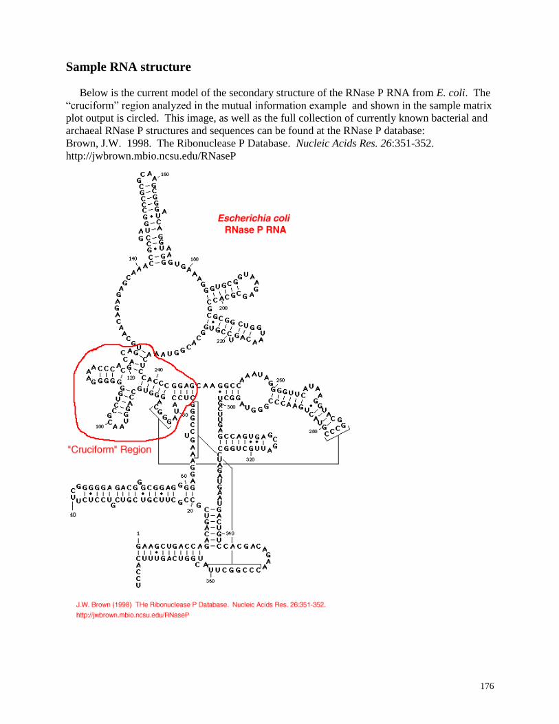
176
Sample RNA structure
Below is the current model of the secondary structure of the RNase P RNA from E. coli. The
“cruciform” region analyzed in the mutual information example and shown in the sample matrix
plot output is circled. This image, as well as the full collection of currently known bacterial and
archaeal RNase P structures and sequences can be found at the RNase P database:
Brown, J.W. 1998. The Ribonuclease P Database. Nucleic Acids Res. 26:351-352.
http://jwbrown.mbio.ncsu.edu/RNaseP
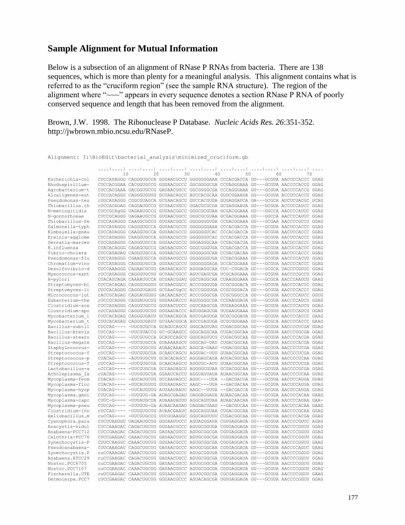
177
Sample Alignment for Mutual Information
Below is a subsection of an alignment of RNase P RNAs from bacteria. There are 138
sequences, which is more than plenty for a meaningful analysis. This alignment contains what is
referred to as the “cruciform region” (see the sample RNA structure). The region of the
alignment where “~~~” appears in every sequence denotes a section RNase P RNA of poorly
conserved sequence and length that has been removed from the alignment.
Brown, J.W. 1998. The Ribonuclease P Database. Nucleic Acids Res. 26:351-352.
http://jwbrown.mbio.ncsu.edu/RNaseP.
Alignment: I:\BioEdit\bacterial_analysis\minimized_cruciform.gb
....|....| ....|....| ....|....| ....|....| ....|....| ....|....| ....|....| ....
10 20 30 40 50 60 70
Escherichia-col CUCCAUAGGG CAGGGUGCCA GGUAACGCCU GGGGGGGAAA CCCACGACCA GU~~~GCGUA AACUCCACCC GGAG
Rhodospirillum- CUCCACGGAA CACGGUGCCG GGUAACGCCC GGCGGGGCGA CCUAGGGAAA GU~~~GCGUA AACCCCACCG GGAG
Agrobacterium-t CUCCACGAAA UACGGUGCCG GAUAACGUCC GGCGGGGCGA CCCAGGGAAA GU~~~GCGUA AACCCCACCG GGAG
Alcaligenes-eut CUCCACAGGG CAGGGUGUUG GCUAACAGCC AUCCACGCAA GUGCGGAAUA GG~~~GCGUA ACCUCCACCU GGAG
Pseudomonas-tes cUGCAUAGGG CGGCGUAGCA GCUAACAGCU GUCCACGUGA GUGAGGAUCA GA~~~GCGCA AUCUCUACGC GCAG
Thiobacillus.th cUCCACAGAG CAGGAUGCCG GCUAACGGCC GGACGCGCGA GCGAGGAAUA GG~~~GCGUA ACCUCCAUCC GGAG
N-meningitidis CUCCGCAgGG UAGAAUGCCG GUUAACGGCC GGGCGCGUAA GCGACGGAAA GU~~~GGCCA AACCCCAUUC GGAG
N-gonnorhoeae CUCCGCAGGG UAGAAUGCCG GUUAACGGCC GGGCGCGUAA GCGACGGAAA GU~~~GGCCA AACCCCAUUC GGAG
Thiobacillus-fe CUCCAUAGGG CAAGGCGCCG GUUAACGGCC GGGGGGGUGA CCUACGGAAA GU~~~GCGAA AACCCCGCCU GGAG
Salmonella-typh CUCCAUAGGG CAGGGUGCCA GGUAACGCCU GGGGGGGAAA CCCACGACCA GU~~~GCGUA AACUCCACCC GGAG
Klebsiella-pneu CUCCAUAGGG CAAGGUGCCA GGUAACGCCU GGGGGGUCAC CCCACGACCA GU~~~GCGUA AACUCCACCC GGAG
Erwinia-agglome CUCCAUAGGG CAAGGUGCCA GGUAACGCCU GGGGGGUCAC CCCACGACCA GU~~~GCGUA AACUCCACCC GGAG
Serratia-marces CUCCAUAGGG CAGGGUGCCA GGUAACGCCU GGGAGGGCAA CCUACGACUA GU~~~GCGUA AACUCCACCC GGAG
H.influenza CUACACAGGG CAGAGUGCCG GAUAACGUCC GGGCGGGUGA CCGACGACCA GU~~~GCGUA AACUCCACUC GUAG
Vibrio-cholera CUCCAUAGAG CAGGGUGCCA GGUAACGCCU GGGGGGGCAA CCUACGACAA GU~~~GCGUA AACUCCACCC GGAG
Pseudomonas-flu CUCCAUAGGG CGAAGUGCCA GGUAAUGCCU GGGGGGGUGA CCUACGGAAA GU~~~GCGUA AACCCCACUU GGAG
Chromatium-vino CUCCAUAGGG CAGGGUGCCA GGUAACGCCU GGGGGGGAGA UCCACGGAAA GU~~~GCGUA AACCCCACCC GGAG
Desulfovibrio-d CUCCAAAGGG CAGAACGCUG GAUAACAUCC AGGGAGGCAA CUC-CGGACA GC~~~GCGCA UACCCCGUUC GGAG
Myxococcus-xant cUCCAGAGGG CAGGGUGCUG GCUAACGGCC AGUCGAGCGA UCGCAGGAAA GU~~~GCGUA AACCCCGCCU GGAG
H-pylori CUACAUUAGA CAAAAUUCCA UCUAACGGAU GGCUAGGCAA CUAAGGGAAA GU~~~GCGCA AACCCAAUUU GAAG
Streptomyces-bi CUCCACAGAG CAGGGUGGUG GCUAACGGCC ACCCGGGUGA CCGCGGGACA GU~~~GCGUA AACCCCACUC GGAG
Streptomyces-li CUCCACAGGG CAGGGUGAUG GCUAaCGgCC ACCCGGGUGA CCGCGGGACA GU~~~GCGUA AACCCCACCC GGAG
Micrococcus-lut cACCGCAGAG CAGGAUGGUG GACAACAUCC ACCCGGGCGA CCGCGGGCCA GU~~~GCGUA AACCCCAUCC GGUG
Eubacterium-the cUCCGCAGGG CAGGAUGCUG GGUAAUACCC AGUGGGGCGA CCUAAGGAUA GU~~~GCGUA AACCCCAUCU GGAG
Clostridium-ace CUCCAUAGGG CAGGGUGCCG GGUAACUCCC GGUCAAGCGA UUGAAGGAAA GU~~~GCGUA AACCCCAUCU GGAG
Clostridium-spo cUCCAUAGGG CAGGGUGCUG GGUAAUACCC AGUGGAGCGA UUUAAGGAAA GU~~~GCGUG AACCCCAUCU GGAG
Mycobacterium_l CUUCACAGAG CAGGGUGAUU GCUAACAGCA AUCCGAGUGA UCGCGGGAUA GU~~~GCGUA AACCCCACCC GAAG
Mycobacterium_t CUUCACAGAG CAGGGUGAUU GCUAACGGCA AUCCGAGUGA UCGCGGGAAA GU~~~GCGCA AACCCCACCC GAAG
Bacillus-subtil CUCCAG---- -UUCGUGCCA GCAGUCAGCU GGGCAGUUAG CUGACGGCAA GU~~~GCGUA AACCCCUCGA GGAG
Bacillus-brevis CUCCAG---- -UUCGUACCG GC-GCAAGCC GGGCAGGCAA CUGACGGCAA GU~~~GCGUA AACCCUGCGA GGAG
Bacillus-stearo CUCCAG---- -UUCGUGCCA GCAUCCAGCU GGGCAGUUCG CUGACGGCAA GU~~~GCGUA AACCCCACGA GGAG
Bacillus-megate CUCCAG---- -UUCGUGCCA GUAAAAAGCU GGGCAG-UAU CUGACGGCAA GU~~~GCGUA AACCCCACGA GGAG
Staphylococcus- cUCCAG---- -UUCGUGCUG AUAACAAAUC AGGCA-UAAU -UGACGGCAA GU~~~GCGUA AACCCCUCGA GGAG
Streptococcus-f cUCCAG---- -UUCGUGCUA GCAAUCAGCU AGGUAC-UUU GUAACGGCAA GU~~~GCGUA AACCCCUCGA GGAG
Streptococcus-p CUACAG---- -AUUGUGCUG GCACACAGCC AGGGAUCAUA AUUACGGCAA GU~~~GCGUA AACCCCUCAA GUAG
Streptococcus-f cUCCAG---- -UUCGUGCUA GCAACAAGCU AGGUGC-AUU GUAACGGCAA GU~~~GCGUA AACCCCUCGA GGAG
Lactobacillus-a cCCCAG---- -UUCGUGCUA GCCAAUAGCU AGGGGCGUAA GCUACGGCAA GU~~~GCGUA AACCCCGCGA GGAG
Acholeplasma_la cUACAG---- -UUUGUGCUA GGAAUCACCU AGGUAUUAUA AUAACGGCAA GU~~~GCGUA AACCCCUCAA GUAG
Mycoplasma-ferm CUACAG---- -AUCAUGCUG GCCAAUAGCC AGGC---UUA --GACGACUA GU~~~GCGUA AACUCCAUGA GUAG
Mycoplasma-floc CUACAG---- -UUCAUGUUG GUUAAUAACC AAGC---UUA --GACGACAA GU~~~GCGUA AACUCCAUGA GUAG
Mycoplasma-hyop CUACAG---- -UUCAUGUUG AUUAAUAAUC AAGC--UUUA --GACGACCA GU~~~GCGUA AACUCCAUGA GUAG
Mycoplasma.geni CUUCAG---- -UUUGUG-UA AUAGCGAGAU UAGGAUGAUA AUAACGACAA GU~~~GCGUA AACUCCACAA GAAG
Mycoplasma-capr CUUC-G---- -UUUAUGCUA AUAAAUAUUU AGGCAGUUAA AUAACAACAA GU~~~GCGUA AACCCCAUAA GAA-
Mycoplasma-pneu CUUCAG---- -UUUGUG-UA AUAACAAGAU UAGGACUAAU --GACGUCAA GU~~~ACGUA AACUCCACAA GAAG
Clostridium-inn cUCCAG---- -UUUGUGCUG AUAACGAAUC AGGCAGGUAA CUGACGGCAA GU~~~GCGUA AACCCCGCAA GGAG
Heliobacillus.m cuCCAG---- -UUCGUGCCG UUCGUAAGGC GGGCAGUUUU CUGACGGCAA GU~~~GGCUA AACCCCACGA GGAG
Cyanophora.para CUCUUAAGGU UAGAAUGCUG GGUAAUUCCC AGUACGGAUA CGUGAGGAUA GU~~~GCGUA AACCCCGUUC AGAG
Anacystis-nidul CUCCAAAGAC CAGACUGCUG GGUAACGCCC AGUGCGGUGA CGUGAGGAGA GU~~~GCGUA AACCCCGGUU GGAG
Anabaena-PCC712 CUCCGAAGAC CAGACUGCUG GAUAACGUCC AGUGCGGCGA CGUGAGGAUA GU~~~GCGUA AACCCCGGUU GGAG
Calothrix-PCC76 CUCCGAAGAC CAAACUGCUG GAUAACGUCC AGUGCGGCGA CGUGAGGAUA GU~~~GCGUA AACCCCGGUU GGAG
Synechocystis-P CUUCCAAGGC CAAACUGCUG GGUAACGCCC AGUGCGGCGA CGUGAGGACA GU~~~GCGUA AACCCCGGUU GAAG
Pseudoanabaena- CUUCAAAGAU CAGGCUGCUG GAUAACGCCC AGUGCGGCAA CGUGAGGAUA GU~~~GCGUA AACCCCAGUC GAAG
Synechocystis.P cuCCAAAGAU CAAACUGCUG GGUAACGCCC AGUGCGGUGA CGUGAGGAUA GU~~~GCGUA AACCCCGGUG GGAG
Anabaena.ATCC29 cuCCGAAGAC CAGACUGCUG GAUAACUUCC AGUGCGGCGA CGUGAGGAUA GU~~~GCGUA AACCCCGGUU GGAG
Nostoc.PCC6705 cuCCGAAGAC CAGACUGCUG GAUAACGUCC AGUGCGGCGA CGUGAGGAUA GU~~~GCGUA AACCCCGGUU GGAG
Nostoc.PCC7107 cuCCGAAGAC CAAACUGCUG GAUAACGUCC AGUGCGGCGA CGUGAGGAUA GU~~~GCGUA AACCCCGGUU GGAG
Fischerella.UTE cuUCGAAGAC CAAACUGCUG GGUAACGCCC AGUGCGGCGA CGCGAGGAUA GU~~~GCGUA AACCCCGGUU GAAG
Dermocarpa.PCC7 cUCCGAAGAC CAAACUGCUG GGUAACGCCC AGUACAGCGA UGUGAGGAUA GU~~~GCGUA AACCCCGGUU GGAG
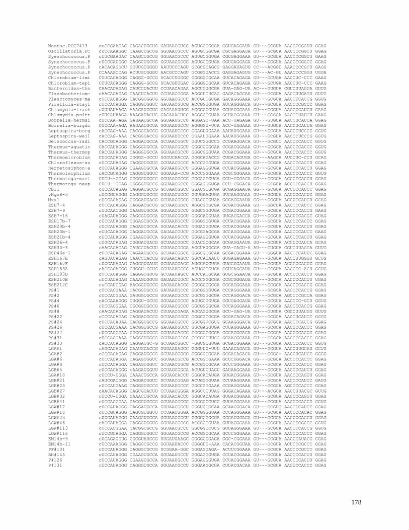
178
Nostoc.PCC7413 cuCCGAAGAC CAGACUGCUG GAUAACGUCC AGUGCGGCGA CGUGAGGAUA GU~~~GCGUA AACCCCGGUU GGAG
Oscillatoria.PC cuCCAAAGGC CAAGCUGCUG GGUAACGCCC AGUGCGGCGA CGCGAGGAUA GU~~~GCGUA AACCCCGGCU GGAG
Syenchococcus.P cUUCGAAGAC CAAGCUGCUG GGUAACGCCC AGUGCGGUGA CGUGAGGAAA GU~~~GCGUA AACCCCGGCU GAAG
Synechococcus.P cUCCCAUGGC CAGGCUGCUG GGUAACGCCC AGUGCGGUGA CGUGAGGAGA GU~~~GCGUA AACCCCGGCC GGAG
Synechococcus.P cACACAGGCU GGUUGUGGGU AAUUCCCAGU GCGCGCAGCG GAGGAUAGUG CC~~~ACGGU AAACCCCGCU GAGG
Synechococcus.P CCAAAGCCAG ACUUGUGGGU AACGCCCAGU GCGGGUACCG GAGGAGAGUG CC~~~AC-GU AAACCCCGGU UGGA
Chlorobium-limi CUUCACAGGG CAGGG-GCCG UCACCUGGGC GGGGGCGCAA GUCACAGAGA GU~~~GCUGA AACCUC-CCC GAAG
Chlorobium-tepi CUUCACAGGG CAGGG-GCCG UCACGUUGAC GGGGGCGCAA GUCACAGAGA GU~~~GCUGA AACCUC-CCC GAAG
Bacteroides-the CAACACAGAG CAUCCUACUU CCUAACAGAA AGCUGUGCGA GUA-GAG-UA AC~~~GUGUA CGUCUUAGGA GUUG
Flavobacterium- cAACACAGAG CAACUCACUU CCUAACGGGA AGGCUCUCAG GAGACAGCAA GU~~~GCGUA AACCUUGAGU GUUG
Planctomyces-ma cUCCACAGGG CACGGUGGUG GGUAACGCCC ACCGUCGCGA GACAGGGAAA GU~~~GCGUA AACCCCACCG GGUG
Pirellula-stayl cUCCACAGGA CAGGGUGGUC GAUAACGUCG ACCGGUGUGA AUCAGGGACA GU~~~GCGUA AACCCCGCCC GGAG
Chlamydia-trach cUUUAUAAGA AAAGAUGCUG GAGAAAUUCC AGGGGCGUAA GCUACGGAAA GU~~~GCGUA AACCCCAUCU GAAG
Chlamydia-psitt cUUCAUAAGA AAAGAUACUG GAGAAACUCC AGGGGCGUAA GCUACGGAAA GU~~~GCGCA AACCCUAUCU GAAG
Borrelia-hermsi cUCCAA-AGA GAUAAUGCUA GGUAAUGCCU AGGAGU-UAA ACU-UAGAGA GU~~~GUGUA AACCUCAUUA GGAG
Borrelia-burgdo CUCCAA-AGA AAUAAUGCUA GGUAAUGCCU AGGGGU-UUA ACC-UAGAAA GU~~~GUGUA AACCUCAUUA GGAG
Leptospira-borg cACCAG-AAA CACGGGACCG GGUAAUCCCC GGAGUUGAAA AAUAUGGAAA GU~~~GCGUA AACCCUCCCG GGUG
Leptospira-weil cACCAG-AAA CACGGGACCG GGUAAUUCCC GGAAUUGAAA AAUAUGGAAA GU~~~GCGUA AACCCUCCCG GGUG
Deincoccus-radi CACCGCAGGG CAGGAUGCCA GCUAACGGCU GGUCGGGCCG CCGAAGGACA GU~~~GCGUC AACCCCAUCC GGUG
Thermus-aquatic CACCAUAGGG CAGGGUGCCA GCUAACGGCU GGGCGGGCAA CCGACGGAAA GU~~~GCGCA AACCCCACCC GGUG
Thermus-thermop CACCAUAGGG CAGGGUGCCA GGUAACGCCU GGGCGGGUAA CCGACGGAAA GU~~~GCGCA AACCCCACCC GGUG
Thermomicrobium CUGCACAGAG CGGGG-GCCU GGGUCAACCA GGGCAGACCG CUGACAGUGA GC~~~AAGCA AUCCUC-CCU GCAG
Chloroflexus-au cUCCAUAGAG CAGGGUGGUG GGUAACGCCC ACCCGGGUGA CCGCGGGAAA GU~~~GCGCA AACCCCACCU GGAG
Herpetosiphon-a cUCCAUAGGG CGAAGUGCCA GGUAAUGCCU GGGAGGGUGA CCUACGGAAA GU~~~GCGCA AACCCCACCU GGAG
Thermoleophilum cACCGCAGGG CAGGGUGGUC GGGAAA-CCG ACCCGGGAAA CCGCGGGAAA GU~~~GCGCA AACCCCACCC GGUG
Thermotoga-mari CUCU--GGAG CGGGGUGCCG GGUAACGCCC GGGAGGGUGA CCU-CGGACA GG~~~GCGCA ACCCCCACCU GGAG
Thermotoga-neap CUCU--GGAG CGGGGUGCCG GGUAACGCCC GGGAGGGUGA CCU-CGGACA GG~~~GCGCA ACCCCCACCU GGAG
vB11 cUCCACAGAG CAGGAUGCCG GCUAACGGCC GGACGCGCGA GCGAGGAAUA GG~~~GCGUA ACCUCCAUCC GGAG
vHge8-3 cUCCGCAGGG CAGGGUGCCG GGUAACUCCC GGUGAAGUGA UUCAAGGAAA GU~~~GCGUA AACCCCACUC GGAG
Mxa1 cUGCACAGAG CGGGAUGACG GCUAACGGCC GUACGCGUAA GCGAGGAAUA GG~~~GCGUA ACCUCCAUCU GCAG
ESH7-4 cUCCACAGGG CAGGAUGCUG GCUAACGGCC AGGCGUGCGA GCGACGGAAA GU~~~GGCUA AACCCCAUCC GGAG
ESH7-9 cUUCAACGGG CAAGGUGCCA GGUAACGCCU GGGCGGGUGA CCGACGGAAA GU~~~GCGUA AACCCCACCG GAAG
ESH7-16 cUACAUAGGG CAGCGUGCCA GCUAACGGCU GGGCAGGUAA UUGACGACCA GU~~~GCGUA AACUCCACGC GUAG
ESH17b-7 cUCCAUAGGG CGGAGUGCCA GGUAAUGCCU GGGGGGGUGA CCUACGGAAA GU~~~GCGUA AACCCCACUC GGAG
ESH20b-4 cUCCAUAGGG CAGAGCGCCA GGUAACACCU GGGAGGGUGA CCUACGGAAA GU~~~GCGUA AACCCCACUU GGAG
ESH20b-1 cUUCACAGGG CAGGAUGCCA GAUAACGUCU GGCGGAGCGA UCCAGGGAAA GU~~~GCGUA AACCCCAUCC GAAG
ESH21b-4 cUCCAUAGGG CGAAGUGCCA GGUAAUGCCU GGGAGGGUGA CCUACGGAAA GU~~~GCGUA AACCCCACUU GGAG
ESH26-4 cUGCACAGAG CGGGAUGACG GCUAACGGCC GUACGCGCAA GCGAGGAAUA GG~~~GCGUA ACCUCCAUCA GCAG
ESH30-3 cAACACAGAG CAUCCUACUU CUUAACGGGA AGCUAUGCGA GUA-GAGU-A AU~~~GUGUA CGUCUUAGGA GUUG
ESH46a-1 cUCCACAGAG CAGAAUGCCG GCUAACGGCC GGGCGCGCAA GCGACGGAAA GU~~~GGGUA AACCCCAUUC GGAG
ESH167E cAGUACAGAG CAACCCACCG GUGAACAGCC GGCCACAAUU GUGAGAGAAA GU~~~GCGUA AACCUUGGGU GCUG
ESH167F cUCCAUAGAG CAGGGUGAUG GCUAACGACC AUCCACGUGA GUGCGGAAUA GG~~~GCGUA ACCGCCACCC GGAG
ESH183A cACCACAGGG CUGGU-GCUG GGUAAUGCCC AGUGCGGUGA CGUGAGGAUA GU~~~GCGUA AACCCC-ACU GGUG
ESH183D cUCCAUAGGG CAGGGUGUUG GCUAAUAGCC AUCCACGCAA GUGCGGAAUA GG~~~GCGUA ACCUCCACCU GGAG
ESH210B cUCUACAGAG CAAAGUGGUG GAUAACUUCC ACCCGGGCGA CCGCGGGAUA GU~~~GCGCA AACCCCACUU UGAG
ESH212C cuCCAUCGAC AACGGUGCCG GAUAACACCC GGCGGGGCGA CCCAGGGAAA GU~~~GCGCA AACCCCACCG GGAG
PS#1 cUCCACGAAA CACGGUGCCG GAUAAUGCCC GGCGGGGUGA CCCAGGGAAA GU~~~GCGCA AACCCCACCG GGAG
PS#2 cUCCACGGAA GAUGGUGCCG GGUAACGCCC GGCGGGGCGA CCCAGGGACA GC~~~GCGCA AGCCCCGCCA GGAG
PS#4 cACCAAAGGG CUGGU-GCUG GGUAACGCCC AGUGCGGUGA CGUGAGGAUA GU~~~GCGUA AACCCC-GCU GGUG
PS#6 cUCCACGGAA CGCGGUGCCG GGUAACGCCC GGCGGGGCGA CCCAGGGAAA GU~~~GCGCA AACCCCACCG GGAG
PS#8 cAACACAGAG CAGGAUACUU CUUAACGAGA AGCAGUGCGA GCU-GAG-UA GU~~~GUGUA CGCCUUAUGG GUUG
PS#22 cCCCACAGAG CAGGAUGCCG GCUAACGGCC GGGCGCGCGA GCGACAGACA GU~~~GCGCA AACCUCAUCC GGGG
PS#24 cUCCACAUAA CACGGUGCCG GGUAACGCCC GGCGGUCGUG GCAAGGGACA GU~~~GCGCA AACCCCACCG GGAG
PS#26 cUCCACGAAA CACGGUGCCG GAUAAUGUCC GGCGAGGUGA CUUAGGGAAA GU~~~GCGCA AACCCCACCC GGAG
PS#27 cUCCACGGAA CGCGGUGCCG GGUAACACCC GGCGGGGCGA CCCAGGGACA GU~~~GCGCA AACCCCACCG GGAG
PS#31 cUCCACGAAA CAGGGUGGCG GGUAACGCCC GCCGGCUUCG GCAAGGGAAA GU~~~GCGCA AACCCCACCC GGAG
PS#33 cACCACAGGG CAGGAUGC-G GCUAACGGCC -GGCGCGUGA GCGACGGAAA GU~~~GCGCA AACCCCAUCC GGUG
LGA#1 cAGCACAGAG CAAUGCACCG GUGAAUAGCC GGGUUC-UUU GAAACAGACA GU~~~GCGUA AACCUUGCAU GCUG
LGA#2 cCCCACAGAG CAGGAUGCCG GCUAACGGCC GGGCGCGCAA GCGACAGACA GU~~~GCGC- AACCUCAUCC GGGG
LGA#6 cUCCACAGGA CAGAGUGGUC GGUAACGCCG ACCGGCGAAA GCUCGGGACA GG~~~GCGCA ACCCCCACUC GGAG
LGA#8 cUCCACAGGA CAGAGUGGUC GCUAACGGCG ACCGGCGCAA GCUCGGGAAA GU~~~GCGCA AACCCCACUC GGAG
LGB#5 cUCCACAGGG cAAGAUGGUU GCUAGCGGCA ACUGUCUAGU GAUAAGGAAA GU~~~GCGUA AACCCCAUCU GGAG
LGA#10 cUCCU-UGGA CAAACUGCCA GGUAGCACCU GGGCACAUGA GUGACGGAAA GU~~~GCGUA AACCCCAGUU GGAG
LGB#21 cAUCGACGGG CAGGAUGGUC UCUAACGGAG ACUGGGGUAA CCUAAGGAAA GU~~~GCGCA AACCCCAUCC GAUG
LGB#23 cUCCAUGAAG CAGGGUGCCG GGUAAUGCCC GGCCGGGAAA CCGAGGGAAA GC~~~GCGCA AGCCCCACCC GGAG
LGB#27 cAACACAGGG CAGCGUACUU CCUAACGGGA AGGCCCUUAG GGGACAGAAA GU~~~ACGCA AACCUUACGC GUUG
LGB#32 cUCCU-UGGA CAAACUGCCA GGUAACACCU GGGCACAUGA GUGACGGAAA GU~~~GCGUA AACCCCAGUU GGAG
LGB#41 cUCCACGGAA CACGGUGCCG GGUAACGCCC GGCGGCCUCG GUUAGGGAAA GU~~~GCGUA AACCCCACCG GGUG
LGW#17 cUCCAUAGGG CAGGAUGCCA GUUAACGGCU GGGUGCGCAA GCAACGGACA GU~~~GCGUG AACCCCAUCC GGAG
LGW#18 cUCCGCAGGG CAGUGUGGUU CCUAACGGGA ACCGGGGUAA CCCAGGGAAA GU~~~GCGUA AACCCCACAC GGAG
LGW#23 cUCCAUAGGG CAAGGUGCCA GGUAACGCCU GGGGGGGCGA CCCACGGACA GU~~~GCGCA AACCCCACCU GGAG
LGW#46 cACCAUAGGA CAGGGUGGUG GGUAACGCCC ACCGGCGUAA GUUAGGGAAA GU~~~GCGUA AACCCCGCCC GGUG
LGW#113 cUCCACGGAA CACGGUGCCG GGUAACGCCC GGCGGCCUCG GUUAGGGAAA GU~~~GCGUA AACCCCACCG GGUG
LGW#116 cUCCGCAGGA CAGGGUGGUC GGUAACGCCG ACCGGCGCAA GCUCGGGAAA GU~~~GCGCA AACCCCACCC GGAG
EM14b-9 cUCAGAGGUG CGCGUAUCCG UUGAUGAAGC GGGGCGGAGA CGC-CGGAAA GU~~~GCGUA AACCCAUACG CGAG
EM14b-11 cUCCAAAGGG CAGGGCGCCG GGUAAUACCC GGGGUG-AAA CACACGGUAA GG~~~GCGUA ACUCCCGCCC GGAG
PF#101 cUCCAUAGGG CAGGGCGCUG UCGGAA-GGC GGGAGUAGA- ACUUCGGAAA GU~~~GCGCA AACCCCGCCC GGAG
BH#145 cUCCAUAGGG CGAAGUGCCA GGUAAUGCCU GGGAGGGUGA CCUACGGAAA GU~~~GCGUA AACCCCACUU GGAG
P#126 cUCCAUAGGG CGAAGUGCCA GGUAAUGCCU GGGAGGGUGA CCUACGGAAA GU~~~GCGUA AACCCCACUU GGAG
P#131 cUCCAUAGGG CAGGGUGCCA GGUAACGCCU GGGAAGGCGA CUUACGACAA GU~~~GCGUA AACUCCACCC GGAG
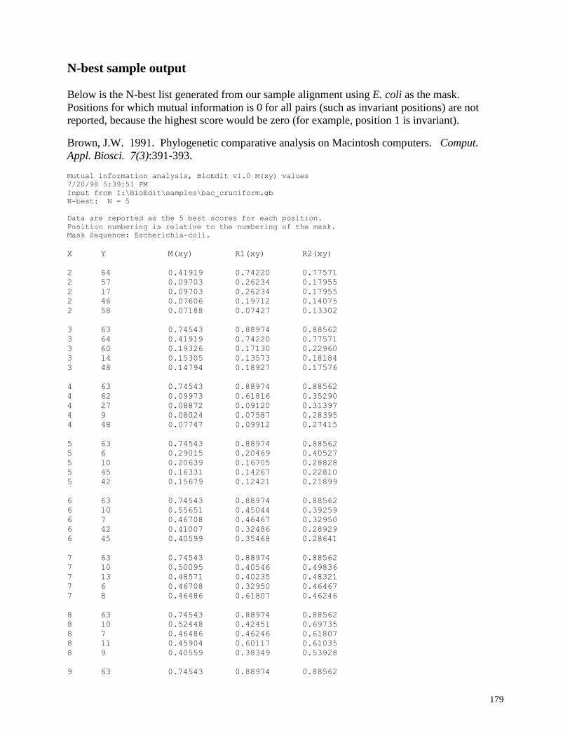
179
N-best sample output
Below is the N-best list generated from our sample alignment using E. coli as the mask.
Positions for which mutual information is 0 for all pairs (such as invariant positions) are not
reported, because the highest score would be zero (for example, position 1 is invariant).
Brown, J.W. 1991. Phylogenetic comparative analysis on Macintosh computers. Comput.
Appl. Biosci. 7(3):391-393. Mutual information analysis, BioEdit v1.0 M(xy) values
7/20/98 5:39:51 PM
Input from I:\BioEdit\samples\bac_cruciform.gb
N-best: N = 5
Data are reported as the 5 best scores for each position.
Position numbering is relative to the numbering of the mask.
Mask Sequence: Escherichia-coli. X Y M(xy) R1(xy) R2(xy)
2 64 0.41919 0.74220 0.77571
2 57 0.09703 0.26234 0.17955
2 17 0.09703 0.26234 0.17955
2 46 0.07606 0.19712 0.14075
2 58 0.07188 0.07427 0.13302
3 63 0.74543 0.88974 0.88562
3 64 0.41919 0.74220 0.77571
3 60 0.19326 0.17130 0.22960
3 14 0.15305 0.13573 0.18184
3 48 0.14794 0.18927 0.17576
4 63 0.74543 0.88974 0.88562
4 62 0.09973 0.61816 0.35290
4 27 0.08872 0.09120 0.31397
4 9 0.08024 0.07587 0.28395
4 48 0.07747 0.09912 0.27415
5 63 0.74543 0.88974 0.88562
5 6 0.29015 0.20469 0.40527
5 10 0.20639 0.16705 0.28828
5 45 0.16331 0.14267 0.22810
5 42 0.15679 0.12421 0.21899
6 63 0.74543 0.88974 0.88562
6 10 0.55651 0.45044 0.39259
6 7 0.46708 0.46467 0.32950
6 42 0.41007 0.32486 0.28929
6 45 0.40599 0.35468 0.28641
7 63 0.74543 0.88974 0.88562
7 10 0.50095 0.40546 0.49836
7 13 0.48571 0.40235 0.48321
7 6 0.46708 0.32950 0.46467
7 8 0.46486 0.61807 0.46246
8 63 0.74543 0.88974 0.88562
8 10 0.52448 0.42451 0.69735
8 7 0.46486 0.46246 0.61807
8 11 0.45904 0.60117 0.61035
8 9 0.40559 0.38349 0.53928
9 63 0.74543 0.88974 0.88562
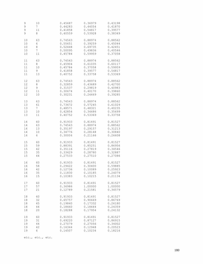
180
9 10 0.45687 0.36979 0.43198
9 7 0.44283 0.44054 0.41870
9 11 0.41858 0.54817 0.39577
9 8 0.40559 0.53928 0.38349
10 63 0.74543 0.88974 0.88562
10 6 0.55651 0.39259 0.45044
10 8 0.52448 0.69735 0.42451
10 7 0.50095 0.49836 0.40546
10 11 0.45784 0.59959 0.37058
11 63 0.74543 0.88974 0.88562
11 8 0.45904 0.61035 0.60117
11 10 0.45784 0.37058 0.59959
11 9 0.41858 0.39577 0.54817
11 13 0.40752 0.33758 0.53369
12 63 0.74543 0.88974 0.88562
12 8 0.32859 0.43689 0.42700
12 9 0.31537 0.29819 0.40983
12 11 0.30674 0.40170 0.39860
12 10 0.30231 0.24469 0.39285
13 63 0.74543 0.88974 0.88562
13 61 0.73672 0.57245 0.61029
13 7 0.48571 0.48321 0.40235
13 10 0.42854 0.34686 0.35499
13 11 0.40752 0.53369 0.33758
14 60 0.91933 0.81491 0.81527
14 63 0.74543 0.88974 0.88562
14 13 0.35197 0.29157 0.31213
14 10 0.34776 0.28148 0.30840
14 6 0.30004 0.21166 0.26608
15 60 0.91933 0.81491 0.81527
15 59 0.88391 0.85251 0.86956
15 42 0.35116 0.27819 0.34546
15 35 0.33429 0.28780 0.32887
15 44 0.27533 0.27510 0.27086
16 60 0.91933 0.81491 0.81527
16 58 0.29422 0.30400 0.59885
16 42 0.12736 0.10089 0.25923
16 35 0.11830 0.10185 0.24079
16 15 0.10383 0.10215 0.21134
17 60 0.91933 0.81491 0.81527
17 57 0.36986 1.00000 1.00000
17 21 0.12789 0.21581 0.34579
18 60 0.91933 0.81491 0.81527
18 32 0.65757 0.90669 0.86769
18 45 0.19840 0.17332 0.26180
18 44 0.18460 0.18444 0.24359
18 20 0.18288 0.17954 0.24132
19 60 0.91933 0.81491 0.81527
19 31 0.69220 0.87127 0.86915
19 44 0.27079 0.27056 0.34002
19 42 0.16344 0.12948 0.20523
19 6 0.14507 0.10234 0.18216
etc., etc., etc.
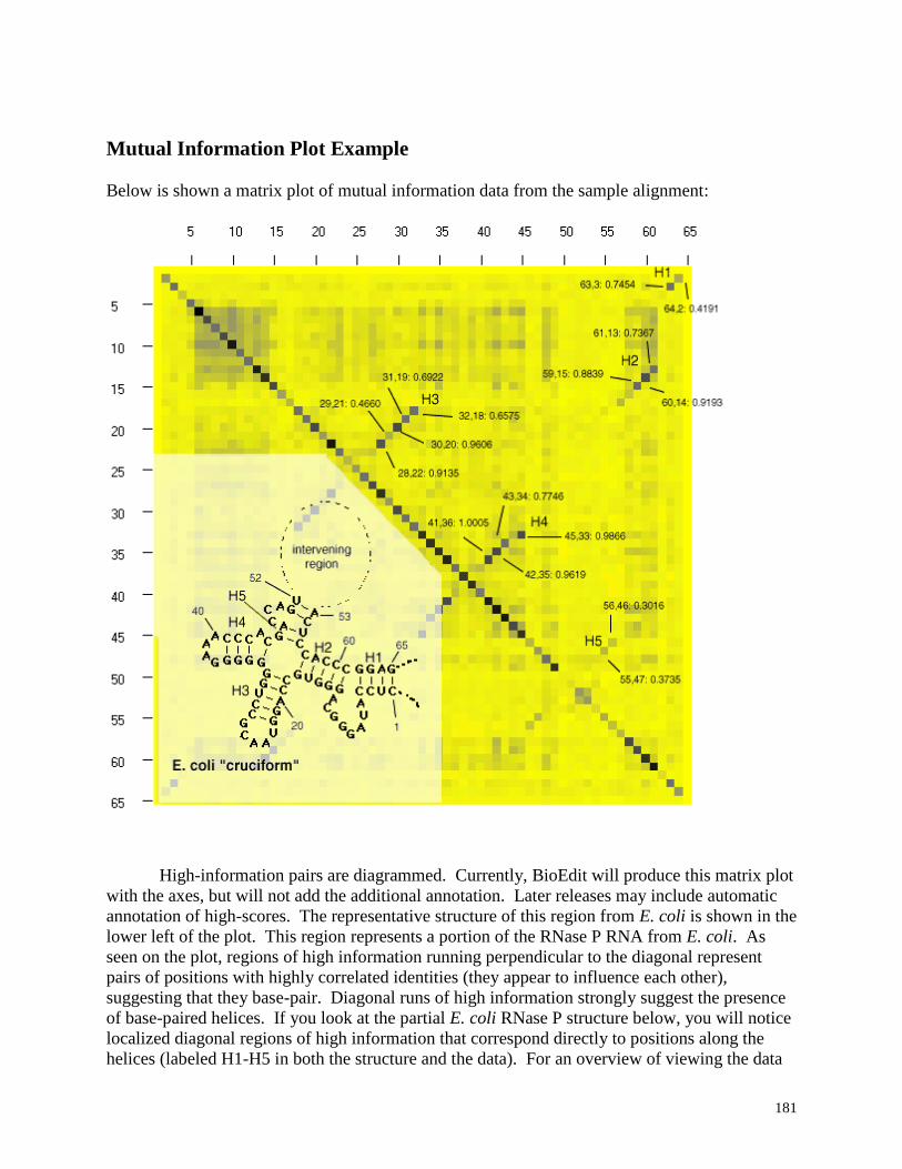
181
Mutual Information Plot Example
Below is shown a matrix plot of mutual information data from the sample alignment:
High-information pairs are diagrammed. Currently, BioEdit will produce this matrix plot
with the axes, but will not add the additional annotation. Later releases may include automatic
annotation of high-scores. The representative structure of this region from E. coli is shown in the
lower left of the plot. This region represents a portion of the RNase P RNA from E. coli. As
seen on the plot, regions of high information running perpendicular to the diagonal represent
pairs of positions with highly correlated identities (they appear to influence each other),
suggesting that they base-pair. Diagonal runs of high information strongly suggest the presence
of base-paired helices. If you look at the partial E. coli RNase P structure below, you will notice
localized diagonal regions of high information that correspond directly to positions along the
helices (labeled H1-H5 in both the structure and the data). For an overview of viewing the data
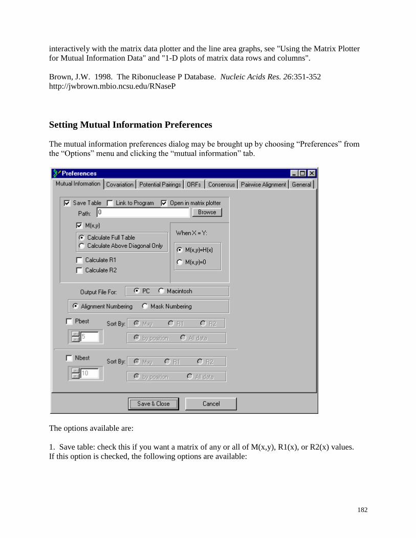
182
interactively with the matrix data plotter and the line area graphs, see "Using the Matrix Plotter
for Mutual Information Data" and "1-D plots of matrix data rows and columns".
Brown, J.W. 1998. The Ribonuclease P Database. Nucleic Acids Res. 26:351-352
http://jwbrown.mbio.ncsu.edu/RNaseP
Setting Mutual Information Preferences
The mutual information preferences dialog may be brought up by choosing “Preferences” from
the “Options” menu and clicking the “mutual information” tab.
The options available are:
1. Save table: check this if you want a matrix of any or all of M(x,y), R1(x), or R2(x) values.
If this option is checked, the following options are available:
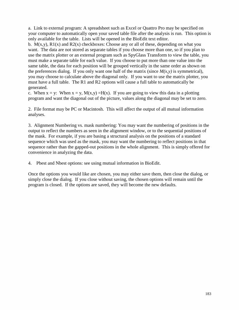
183
a. Link to external program: A spreadsheet such as Excel or Quattro Pro may be specified on
your computer to automatically open your saved table file after the analysis is run. This option is
only available for the table. Lists will be opened in the BioEdit text editor.
b. M(x,y), R1(x) and R2(x) checkboxes: Choose any or all of these, depending on what you
want. The data are not stored as separate tables if you choose more than one, so if you plan to
use the matrix plotter or an external program such as SpyGlass Transform to view the table, you
must make a separate table for each value. If you choose to put more than one value into the
same table, the data for each position will be grouped vertically in the same order as shown on
the preferences dialog. If you only want one half of the matrix (since M(x,y) is symmetrical),
you may choose to calculate above the diagonal only. If you want to use the matrix plotter, you
must have a full table. The R1 and R2 options will cause a full table to automatically be
generated.
c. When x = y: When x = y, M(x,y) =H(x). If you are going to view this data in a plotting
program and want the diagonal out of the picture, values along the diagonal may be set to zero.
2. File format may be PC or Macintosh. This will affect the output of all mutual information
analyses.
3. Alignment Numbering vs. mask numbering: You may want the numbering of positions in the
output to reflect the numbers as seen in the alignment window, or to the sequential positions of
the mask. For example, if you are basing a structural analysis on the positions of a standard
sequence which was used as the mask, you may want the numbering to reflect positions in that
sequence rather than the gapped-out positions in the whole alignment. This is simply offered for
convenience in analyzing the data.
4. Pbest and Nbest options: see using mutual information in BioEdit.
Once the options you would like are chosen, you may either save them, then close the dialog, or
simply close the dialog. If you close without saving, the chosen options will remain until the
program is closed. If the options are saved, they will become the new defaults.
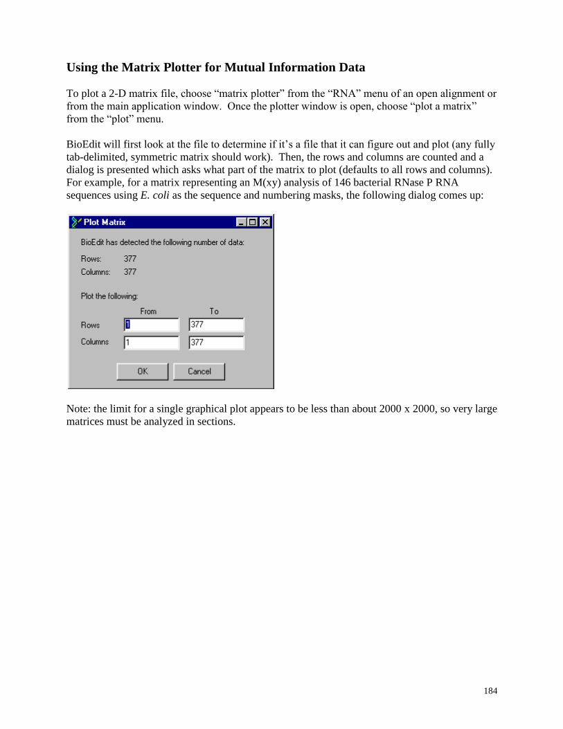
184
Using the Matrix Plotter for Mutual Information Data
To plot a 2-D matrix file, choose “matrix plotter” from the “RNA” menu of an open alignment or
from the main application window. Once the plotter window is open, choose “plot a matrix”
from the “plot” menu.
BioEdit will first look at the file to determine if it’s a file that it can figure out and plot (any fully
tab-delimited, symmetric matrix should work). Then, the rows and columns are counted and a
dialog is presented which asks what part of the matrix to plot (defaults to all rows and columns).
For example, for a matrix representing an M(xy) analysis of 146 bacterial RNase P RNA
sequences using E. coli as the sequence and numbering masks, the following dialog comes up:
Note: the limit for a single graphical plot appears to be less than about 2000 x 2000, so very large
matrices must be analyzed in sections.
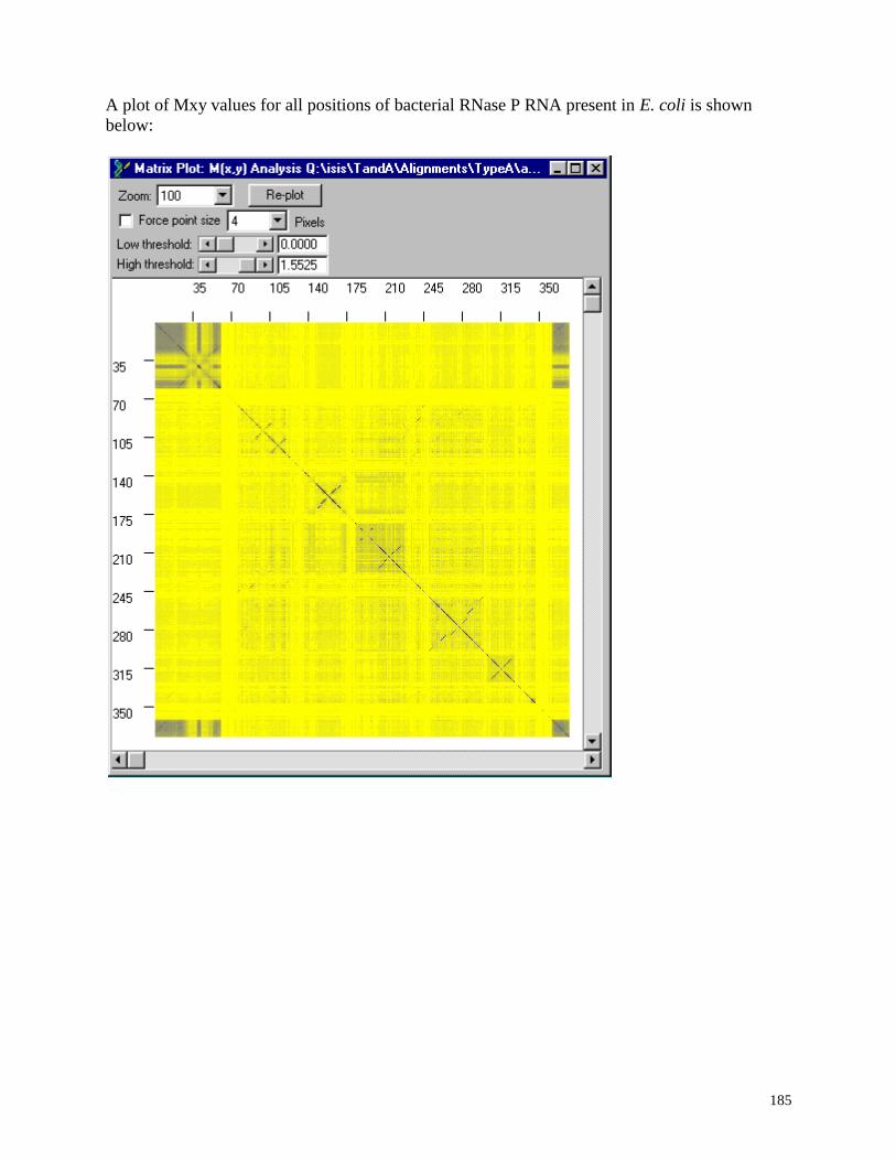
185
A plot of Mxy values for all positions of bacterial RNase P RNA present in E. coli is shown
below:
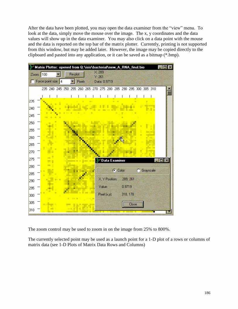
186
After the data have been plotted, you may open the data examiner from the “view” menu. To
look at the data, simply move the mouse over the image. The x, y coordinates and the data
values will show up in the data examiner. You may also click on a data point with the mouse
and the data is reported on the top bar of the matrix plotter. Currently, printing is not supported
from this window, but may be added later. However, the image may be copied directly to the
clipboard and pasted into any application, or it can be saved as a bitmap (*.bmp).
The zoom control may be used to zoom in on the image from 25% to 800%.
The currently selected point may be used as a launch point for a 1-D plot of a rows or columns of
matrix data (see 1-D Plots of Matrix Data Rows and Columns)
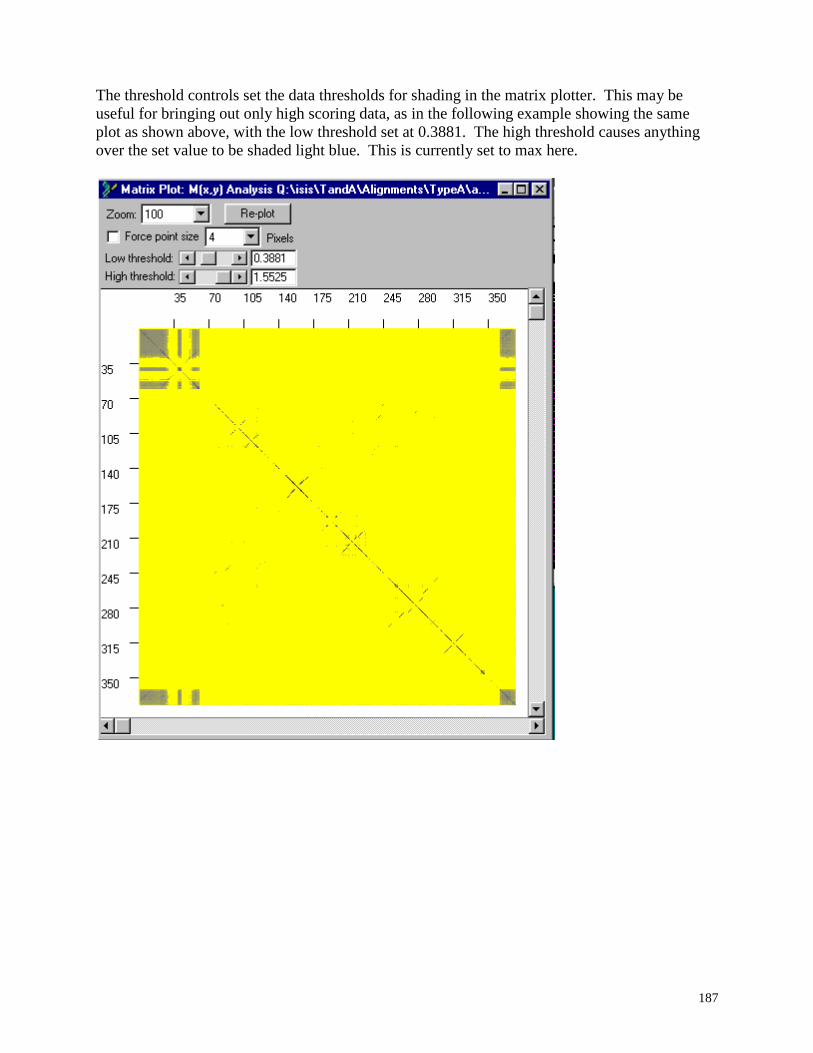
187
The threshold controls set the data thresholds for shading in the matrix plotter. This may be
useful for bringing out only high scoring data, as in the following example showing the same
plot as shown above, with the low threshold set at 0.3881. The high threshold causes anything
over the set value to be shaded light blue. This is currently set to max here.
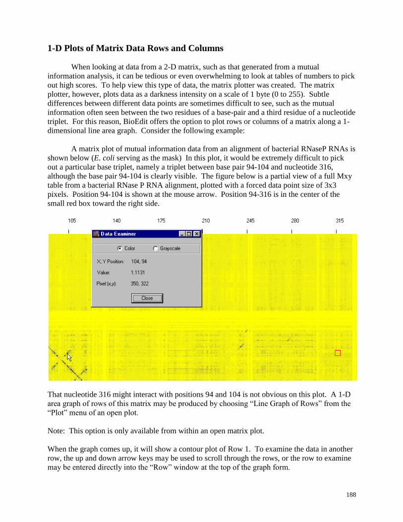
188
1-D Plots of Matrix Data Rows and Columns
When looking at data from a 2-D matrix, such as that generated from a mutual
information analysis, it can be tedious or even overwhelming to look at tables of numbers to pick
out high scores. To help view this type of data, the matrix plotter was created. The matrix
plotter, however, plots data as a darkness intensity on a scale of 1 byte (0 to 255). Subtle
differences between different data points are sometimes difficult to see, such as the mutual
information often seen between the two residues of a base-pair and a third residue of a nucleotide
triplet. For this reason, BioEdit offers the option to plot rows or columns of a matrix along a 1-
dimensional line area graph. Consider the following example:
A matrix plot of mutual information data from an alignment of bacterial RNaseP RNAs is
shown below (E. coli serving as the mask) In this plot, it would be extremely difficult to pick
out a particular base triplet, namely a triplet between base pair 94-104 and nucleotide 316,
although the base pair 94-104 is clearly visible. The figure below is a partial view of a full Mxy
table from a bacterial RNase P RNA alignment, plotted with a forced data point size of 3x3
pixels. Position 94-104 is shown at the mouse arrow. Position 94-316 is in the center of the
small red box toward the right side.
That nucleotide 316 might interact with positions 94 and 104 is not obvious on this plot. A 1-D
area graph of rows of this matrix may be produced by choosing “Line Graph of Rows” from the
“Plot” menu of an open plot.
Note: This option is only available from within an open matrix plot.
When the graph comes up, it will show a contour plot of Row 1. To examine the data in another
row, the up and down arrow keys may be used to scroll through the rows, or the row to examine
may be entered directly into the “Row” window at the top of the graph form.
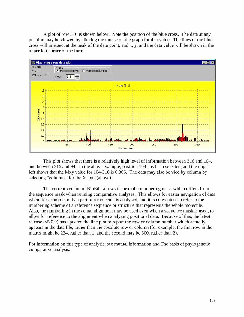
189
A plot of row 316 is shown below. Note the position of the blue cross. The data at any
position may be viewed by clicking the mouse on the graph for that value. The lines of the blue
cross will intersect at the peak of the data point, and x, y, and the data value will be shown in the
upper left corner of the form.
This plot shows that there is a relatively high level of information between 316 and 104,
and between 316 and 94. In the above example, position 104 has been selected, and the upper
left shows that the Mxy value for 104-316 is 0.306. The data may also be vied by column by
selecting “columns” for the X-axis (above).
The current version of BioEdit allows the use of a numbering mask which differs from
the sequence mask when running comparative analyses. This allows for easier navigation of data
when, for example, only a part of a molecule is analyzed, and it is convenient to refer to the
numbering scheme of a reference sequence or structure that represents the whole molecule.
Also, the numbering in the actual alignment may be used even when a sequence mask is used, to
allow for reference to the alignment when analyzing positional data. Because of this, the latest
release (v5.0.0) has updated the line plot to report the row or column number which actually
appears in the data file, rather than the absolute row or column (for example, the first row in the
matrix might be 234, rather than 1, and the second may be 300, rather than 2).
For information on this type of analysis, see mutual information and The basis of phylogenetic
comparative analysis.
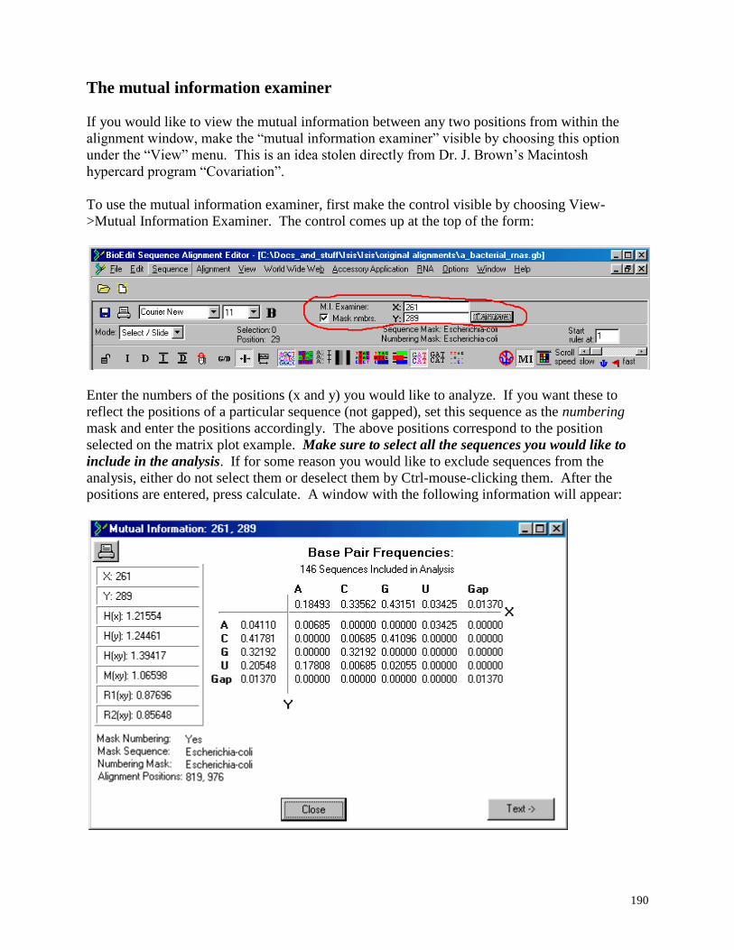
190
The mutual information examiner
If you would like to view the mutual information between any two positions from within the
alignment window, make the “mutual information examiner” visible by choosing this option
under the “View” menu. This is an idea stolen directly from Dr. J. Brown’s Macintosh
hypercard program “Covariation”.
To use the mutual information examiner, first make the control visible by choosing View-
>Mutual Information Examiner. The control comes up at the top of the form:
Enter the numbers of the positions (x and y) you would like to analyze. If you want these to
reflect the positions of a particular sequence (not gapped), set this sequence as the numbering
mask and enter the positions accordingly. The above positions correspond to the position
selected on the matrix plot example. Make sure to select all the sequences you would like to
include in the analysis. If for some reason you would like to exclude sequences from the
analysis, either do not select them or deselect them by Ctrl-mouse-clicking them. After the
positions are entered, press calculate. A window with the following information will appear:
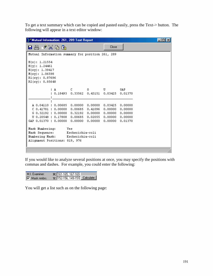
191
To get a text summary which can be copied and pasted easily, press the Text-> button. The
following will appear in a text editor window:
If you would like to analyze several positions at once, you may specify the positions with
commas and dashes. For example, you could enter the following:
You will get a list such as on the following page:
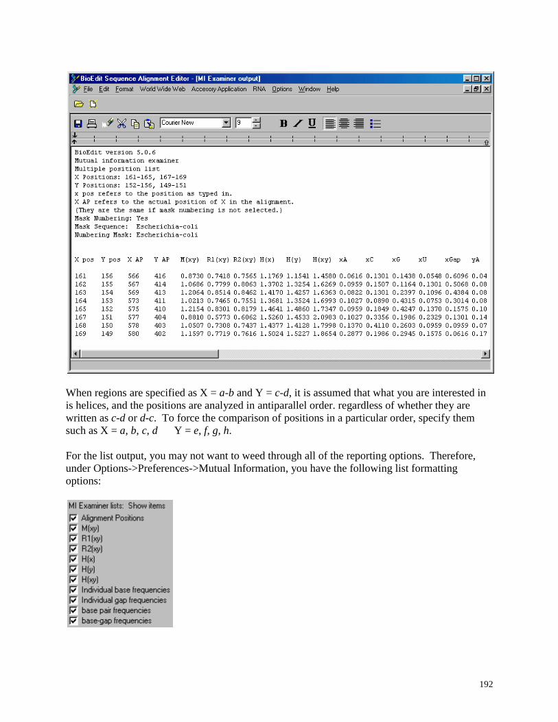
192
When regions are specified as X = a-b and Y = c-d, it is assumed that what you are interested in
is helices, and the positions are analyzed in antiparallel order. regardless of whether they are
written as c-d or d-c. To force the comparison of positions in a particular order, specify them
such as X = a, b, c, d Y = e, f, g, h.
For the list output, you may not want to weed through all of the reporting options. Therefore,
under Options->Preferences->Mutual Information, you have the following list formatting
options: