Bilinear discretization of quadratic vector fieldsBilinear discretization of quadratic vector ﬁelds Yuri B. Suris (Technische Universität Berlin) Oberwolfach Workshop “Geometric

Bilinear discretization of quadratic vectorfields

Yuri B. Suris

(Technische Universität Berlin)

Oberwolfach Workshop “Geometric Integration”, MFO, 24.03.2011

Yuri B. Suris Kahan-Hirota-Kimura Discretizations

Kahan’s discretization

I W. Kahan. Unconventional numerical methods fortrajectory calculations (Unpublished lecture notes, 1993).

x = Q(x) + Bx + c (x − x)/ε = Q(x , x) + B(x + x)/2 + c,

where B ∈ Rn×n, c ∈ Rn, each component of Q : Rn → Rn is aquadratic form, and Q(x , x) = (Q(x + x)−Q(x)−Q(x))/2 isthe corresponding symmetric bilinear function. Thus,

xk (xk − xk )/ε, x2k xk xk , xjxk (xj xk + xjxk )/2.

Note: equations for x always linear, the map x = f (x , ε) isalways reversible and birational,

f−1(x , ε) = f (x ,−ε).


Illustration: Lotka-Volterra system

Kahan’s integrator for the Lotka-Volterra system:{x = x(1− y),

y = y(x − 1),

{x − x = ε(x + x)− ε(xy + xy),

y − y = ε(xy + xy)− ε(y + y).

Explicitly: x = x

(1 + ε)2 − ε(1 + ε)x − ε(1− ε)y1− ε2 − ε(1− ε)x + ε(1 + ε)y

,

y = y(1− ε)2 + ε(1 + ε)x + ε(1− ε)y1− ε2 − ε(1− ε)x + ε(1 + ε)y

.


0.4 0.6 0.8 1.0 1.2 1.4 1.6 1.80.4

0.6

0.8

1.0

1.2

1.4

1.6

1.8

Left: three orbits of Kahan’s discretization with ε = 0.1,right: one orbit of the explicit Euler with ε = 0.01.I J.M. Sanz-Serna. An unconventional symplectic integrator

of W.Kahan. Applied Numer. Math. 16 (1994) 245–250.A sort of an explanation of a non-spiralling behavior: Kahan’sintegrator for the Lotka-Volterra system is symplectic (Poisson).


The problem of integrable discretization. Hamiltonianapproach (Birkhäuser, 2003)

Consider a completely integrable flow

x = f (x) = {H, x} (1)

with a Hamilton function H on a Poisson manifold P with aPoisson bracket {·, ·}. Thus, the flow (1) possesses manyfunctionally independent integrals Ik (x) in involution.

The problem of integrable discretization: find a family ofdiffeomorphisms P → P,

x = Φ(x ; ε), (2)

depending smoothly on a small parameter ε > 0, with thefollowing properties:


1. The maps (2) approximate the flow (1):

Φ(x ; ε) = x + εf (x) + O(ε2).

2. The maps (2) are Poisson w. r. t. the bracket {·, ·} or someits deformation {·, ·}ε = {·, ·}+ O(ε).

3. The maps (2) are integrable, i.e. possess the necessarynumber of independent integrals in involution,Ik (x ; ε) = Ik (x) + O(ε).

While integrable lattice systems (like Toda or Volterra lattices)can be discretized in a systematic way (based, e.g., on ther -matrix structure), there is no systematic way to obtain decentintegrable discretizations for integrable systems of classicalmechanics.


Missing in the book: Hirota-Kimura discretizations

I R.Hirota, K.Kimura. Discretization of the Euler top. J. Phys.Soc. Japan 69 (2000) 627–630,

I K.Kimura, R.Hirota. Discretization of the Lagrange top. J.Phys. Soc. Japan 69 (2000) 3193–3199.

Reasons for this omission: discretization of the Euler topseemed to be an isolated curiosity; discretization of theLagrange top seemed to be completely incomprehensible, if noteven wrong.

Renewed interest stimulated by a talk by T. Ratiu at theOberwolfach Workshop “Geometric Integration”, March 2006,who claimed that HK-type discretizations for the Clebschsystem and for the Kovalevsky top are also integrable.


Hirota-Kimura’s discrete time Euler top

x1 = α1x2x3,

x2 = α2x3x1,

x3 = α3x1x2,

x1 − x1 = εα1(x2x3 + x2x3),

x2 − x2 = εα2(x3x1 + x3x1),

x3 − x3 = εα3(x1x2 + x1x2).

Features:I Equations are linear w.r.t. x = (x1, x2, x3)T:

A(x , ε)x = x , A(x , ε) =

1 −εα1x3 −εα1x2−εα2x3 1 −εα2x1−εα3x2 −εα3x1 1

,

result in an explicit (rational) map, which is reversible(therefore birational):

x = f (x , ε) = A−1(x , ε)x , f−1(x , ε) = f (x ,−ε).


I Explicit formulas rather messy:

x1 =x1 + 2εα1x2x3 + ε2x1(−α2α3x2

1 + α3α1x22 + α1α2x2

3 )

∆(x , ε),

x2 =x2 + 2εα2x3x1 + ε2x2(α2α3x2

1 − α3α1x22 + α1α2x2

3 )

∆(x , ε),

x3 =x3 + 2εα3x1x2 + ε2x3(α2α3x2

1 + α3α1x22 − α1α2x2

3 )

∆(x , ε),

where ∆(x , ε) = det A(x , ε)

= 1− ε2(α2α3x21 + α3α1x2

2 + α1α2x23 )− 2ε3α1α2α3x1x2x3.

(Try to see reversibility directly from these formulas!)


I Two independent integrals:

I1(x , ε) =1− ε2α2α3x2

1

1− ε2α3α1x22, I2(x , ε) =

1− ε2α3α1x22

1− ε2α1α2x23.

I Invariant volume form:

ω =dx1 ∧ dx2 ∧ dx3

φ(x), φ(x) = 1− ε2αiαjx2

k

and bi-Hamiltonian structure found in:M. Petrera, Yu. Suris. On the Hamiltonian structure of theHirota-Kimura discretization of the Euler top. Math. Nachr.,2010, 283, 1654–1663, arXiv:0707.4382 [math-ph].


Hirota-Kimura’s discrete time Lagrange top

Equations of motion of the Lagrange top:

m1 = (α− 1)m2m3 + γp2,

m2 = (1− α)m1m3 − γp1,

m3 = 0,p1 = αp2m3 − p3m2,

p2 = p3m1 − αp1m3,

p3 = p1m2 − p2m1.

It is Hamiltonian w.r.t. Lie-Poisson bracket of e(3), has fourfunctionally independent integrals in involution: two Casimirfunctions,

C1 = p21 + p2

2 + p23, C2 = m1p1 + m2p2 + m3p3,

the Hamilton function, and the (trivial) “fourth integral”,

H1 =12

(m21 + m2

2 + αm23) + γp3, H2 = m3.


Discretization:

m1 −m1 = ε(α− 1)(m2m3 + m2m3) + εγ(p2 + p2),

m2 −m2 = ε(1− α)(m1m3 + m1m3)− εγ(p1 + p1),

m3 −m3 = 0,p1 − p1 = εα(p2m3 + p2m3)− ε(p3m2 + p3m2),

p2 − p2 = ε(p3m1 + p3m1)− εα(p1m3 + p1m3),

p3 − p3 = ε(p1m2 + p1m2 − p2m1 − p2m1).

As usual, this gives an explicit birational map (m, p) = f (m,p, ε).The trivial conserved quantity m3 = const. Quite nontrivial tofind any further conserved quantity!


Hirota-Kimura’s “method” for finding integrals

Consider the expression A = m21 + m2

2 − Bp3 − Cp23, and

determine A,B,C by requiring that they are conservedquantities. For this aim, solve the system of three equations forthese three unknowns:

A + Bp3 + Cp23 = m2

1 + m22,

A + Bp3 + Cp23 = m2

1 + m22,

A + B p˜3 + C p˜23 = m˜ 2

1 + m˜ 22

with (m, p) = f (m,p, ε) and ( m˜ , p˜) = f−1(m,p, ε). Then checkthat A,B,C = A,B,C(m,p, ε) are conserved quantities, indeed.Proceed similarly to determine the conserved quantitiesD, . . . ,M from

D = m1p1 + m2p2 − Ep3 − Fp23, K = p2

1 + p22 − Lp3 −Mp2

3.

Does this make any sense for you???


Nevertheless, Hirota-Kimura’s “method” turns out to be valid inthis case and also for remarkably many other Hirota-Kimuratype discretizations.

How should it be interpreted? Solve (symbolically) the system

(A + Bp3 + Cp23) ◦ f i(m,p, ε) = (m2

1 + m22) ◦ f i(m,p, ε)

with i = −1,0,1. Verify that A = A ◦ f , B = B ◦ f , C = C ◦ f .Alternatively, solve another copy of the above system withi = 0,1,2, and check that the solutions coincide. But then thissystem should be satisfied for all i ∈ Z. In other words, for any(m,p) ∈ R6, certain linear combination

A + Bp3 + Cp23 − (m2

1 + m22)

vanishes along the orbit of (m,p) under the map f .This is a very special feature of both the map f and the set offunctions (1,p3,p2

3,m21 + m2

2). Also the sets of functions

(1,p3,p23,m1p1 + m2p2), (1,p3,p2

3,p21 + p2

2)

have this property. It is formalized in the following definition.Yuri B. Suris Kahan-Hirota-Kimura Discretizations

Hirota-Kimura bases

Definition. For a given birational map f : Rn → Rn, a set offunctions Φ = (ϕ1, . . . , ϕl), linearly independent over R, iscalled a HK-basis, if for every x0 ∈ Rn there exists a vectorc = (c1, . . . , cl) 6= 0 such that

c1ϕ1(f i(x0)) + . . .+ clϕl(f i(x0)) = 0 ∀i ∈ Z.

For a given x0 ∈ Rn, the set of all vectors c ∈ Rl with thisproperty will be denoted by KΦ(x0) and called the null-space ofthe basis Φ (at the point x0). This set clearly is a vector space.

Note: we cannot claim that h = c1ϕ1 + ...+ clϕl is an integral ofmotion, since vectors c ∈ KΦ(x0) vary from one initial point x0 toanother.However: existence of a HK-basis Φ with dim KΦ(x0) = dconfines the orbits of f to (n − d)-dimensional invariant sets.


From HK-bases to integrals

Proposition. If Φ is a HK-basis for a map f , thenKΦ(f (x0)) = KΦ(x0).

Thus, the d-dimensional null-space KΦ(x0) is a Gr(d , l)-valuedintegral. Its Plücker coordinates are scalar integrals.

Especially simple is the situation when the null-space of aHK-basis has dimension d = 1.

Corollary. Let Φ be a HK-basis for f with dim KΦ(x0) = 1 for allx0 ∈ Rn. Let KΦ(x0) = [c1(x0) : . . . : cl(x0)] ∈ RPl−1. Then thefunctions cj/ck are integrals of motion for f .

In other words, normalizing cl(x0) = 1 (say), we find that allother cj (j = 1, . . . , l − 1) are integrals of motion. It is not clearwhether one can say something general about the number offunctionally independent integrals among them. It varies inexamples (sometimes just = 1 and sometimes > 1).


Hirota-Kimura bases for the discrete Lagrange top

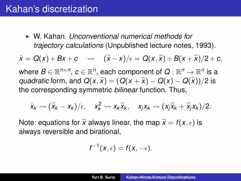
Thus, results by Hirota and Kimura in the Lagrange top casecan be put as follows:

Theorem. The three sets of functions,

Φ1 = (m21 + m2

2, p23, p3, 1),

Φ2 = (m1p1 + m2p2, p23, p3, 1),

Φ3 = (p21 + p2

2, p23, p3, 1),

are HK-bases for the discrete time Lagrange top withone-dimensional null-spaces.

It follows that any orbit lies on a two-dimensional surface in R6

which is intersection of three quadrics and a hyperplanem3 = const .


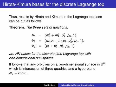
An impression about the complexity of the integrals thus foundcan be given by this: KΦ1(x) = [c0 : c1 : c2 : −1], with

c0 =m2

1 + m22 + 2γp3 + ε2c(4)

0 + ε4c(6)0 + ε6c(8)

0 + ε8c(10)0

∆1∆2,

(and similar expressions for c1, c2), where

∆1 = 1 + ε2α(1− α)m23 − ε2γp3,

∆2 = 1 + ε2∆(2)2 + ε4∆

(4)2 + ε6∆

(6)2 ;

coefficients ∆(q) and c(q)k are polynomials of degree q in the

phase variables.


A simple integral (unnoticed by Hirota and Kimura) is given by:Theorem. The set

Γ = (m1p1 −m1p1, m2p2 −m2p2, m3p3 −m3p3)

is a HK-basis for the discrete time Lagrange top withone-dimensional null-space KΓ(x) = [1 : 1 : I ],

I =(2α− 1) + ε2(α− 1)(m2

1 + m22) + ε2γ(m1p1 + m2p2)/m3

1 + ε2α(1− α)m23 − ε2γp3

.

Another result which was unknown to Hirota and Kimura reads:Theorem. The discrete time Lagrange top possesses aninvariant volume form:

f ∗ω = ω, ω =dm1 ∧ dm2 ∧ dm3 ∧ dp1 ∧ dp2 ∧ dp3

∆2(m,p).


Further examples of integrable HK-discretizations

Work in progress with A. Pfadler, M. Petrera. An overview givenin arXiv:1008.1040 [nlin.SI] (to appear in Regular andChaotic Dyn.). An (incomplete) list of examples:I Three-wave interaction system.I Periodic Volterra chain of period N = 3,4:

xk = xk (xk+1 − xk−1), k ∈ Z/NZ

I Dressing chain with N = 3:

xk + xk+1 = x2k+1 − x2

k + αk+1 − αk , k ∈ Z/NZ, N odd.

I System of two interacting Euler tops.I Kirchhof and Clebsch cases of the rigid body motion in an

ideal fluid.


Clebsch case

Clebsch case of the motion of a rigid body in an ideal fluid:

m1 = (ω3 − ω2)p2p3,

m2 = (ω1 − ω3)p3p1,

m3 = (ω2 − ω1)p1p2,

p1 = m3p2 −m2p3,

p2 = m1p3 −m3p1,

p3 = m2p1 −m1p2.

It is Hamiltonian w.r.t. Lie-Poisson bracket of e(3), has fourfunctionally independent integrals in involution:

Ii = p2i +

m2j

ωk − ωi+

m2k

ωj − ωi, (i , j , k) = c.p.(1,2,3),

and H4 = m1p1 + m2p2 + m3p3.Yuri B. Suris Kahan-Hirota-Kimura Discretizations

Hirota-Kimura discretization of the Clebsch system

Hirota-Kimura-type discretization (proposed by T. Ratiu onOberwolfach Meeting “Geometric Integration”, March 2006):

m1 −m1 = ε(ω3 − ω2)(p2p3 + p2p3),

m2 −m2 = ε(ω1 − ω3)(p3p1 + p3p1),

m3 −m3 = ε(ω2 − ω1)(p1p2 + p1p2),

p1 − p1 = ε(m3p2 + m3p2)− ε(m2p3 + m2p3),

p2 − p2 = ε(m1p3 + m1p3)− ε(m3p1 + m3p1),

p3 − p3 = ε(m2p1 + m2p1)− ε(m1p2 + m1p2).

What follows is based on: M. Petrera, A. Pfadler, Yu. Suris. Onintegrability of Hirota-Kimura type discretizations. Experimentalstudy of the discrete Clebsch system. Experimental Math.,2009, 18, 223–247, arXiv:0808.3345 [nlin.SI]


A birational map(mp

)= f (m,p, ε) = M−1(m,p, ε)

(mp

),

M(m,p, ε) =

1 0 0 0 εω23p3 εω23p20 1 0 εω31p3 0 εω31p10 0 1 εω12p2 εω12p1 00 εp3 −εp2 1 −εm3 εm2−εp3 0 εp1 εm3 1 −εm1εp2 −εp1 0 −εm2 εm1 1

,

with ωij = ωi − ωj . The usual reversibility:

f−1(m,p, ε) = f (m,p,−ε).

Numerators and denominators of components of m, p arepolynomials of degree 6, the numerators of pi consist of 31monomials, the numerators of mi consist of 41 monomials, thecommon denominator consists of 28 monomials.


Phase portraits

0.650.7

0.750.8

0.850.9

0.951

−1

−0.5

0

0.5

1−1

−0.5

0

0.5

1

0.5

1

1.5

−0.8−0.6−0.4−0.200.20.40.60.8−0.5

−0.4

−0.3

−0.2

−0.1

0

0.1

0.2

0.3

0.4

0.5

An orbit of the discrete Clebsch system with ω1 = 0.1, ω2 = 0.2,ω3 = 0.3 and ε = 1; projections to (m1,m2,m3) and to(p1,p2,p3); initial point (m0,p0) = (1,1,1,1,1,1).


−8 −6 −4 −2 0 2 4 6 8−10

0

10

−1.5

−1

−0.5

0

0.5

1

1.5

−3

−2

−1

0

1

2

3

−0.50

0.51

1.52

2.5−1.5

−1

−0.5

0

0.5

1

1.5

An orbit of the discrete Clebsch system with ω1 = 1, ω2 = 0.2,ω3 = 30 and ε = 1; projections to (m1,m2,m3) and to(p1,p2,p3); initial point (m0,p0) = (1,1,1,1,1,1).


Results for the discrete Clebsch system

Theorem. a) The set of functions

Φ = (p21,p

22,p

23,m

21,m

22,m

23,m1p1,m2p2,m3p3,1)

is a HK-basis for f , with dim KΦ(m,p) = 4. Thus, any orbit of flies on an intersection of four quadrics in R6.b) The following four sets of functions are HK-bases for f withone-dimensional null-spaces:

Φ0 = (p21,p

22,p

23,1),

Φ1 = (p21,p

22,p

23,m

21,m

22,m

23,m1p1),

Φ2 = (p21,p

22,p

23,m

21,m

22,m

23,m2p2),

Φ3 = (p21,p

22,p

23,m

21,m

22,m

23,m3p3).

There holds: KΦ = KΦ0 ⊕ KΦ1 ⊕ KΦ2 ⊕ KΦ3 .


HK-basis Φ0

Theorem. At each point (m,p) ∈ R6 there holds:

KΦ0(m,p) =

[1J0

+ ε2ω1 :1J0

+ ε2ω2 :1J0

+ ε2ω3 : −1],

where

J0(m,p, ε) =p2

1 + p22 + p2

3

1− ε2(ω1p21 + ω2p2

2 + ω3p23).

This function is an integral of motion of the map f .This is the only “simple” integral of f !


HK-bases Φ1,Φ2,Φ3

Theorem. At each point (m,p) ∈ R6 there holds:

KΦ1(m,p) = [α1 : α2 : α3 : α4 : α5 : α6 : −1],

KΦ2(m,p) = [β1 : β2 : β3 : β4 : β5 : β6 : −1],

KΦ3(m,p) = [γ1 : γ2 : γ3 : γ4 : γ5 : γ6 : −1],

where αj ,βj , and γj are rational functions of (m,p), even withrespect to ε. They are integrals of motion of the map f . Forj = 1,2,3 they are of the form

h =h(2) + ε2h(4) + ε4h(6) + ε6h(8) + ε8h(10) + ε10h(12)

2ε2(p21 + p2

2 + p23)∆

,

∆ = m1p1 + m2p2 + m3p3 + ε2∆(4) + ε4∆(6) + ε6∆(8),

where h stands for any of the functions αj , βj , γj , j = 1,2,3, andthe corresponding h(2q) and ∆(2q) are homogeneouspolynomials in phase variables of degree 2q. For instance,


HK-bases Φ1,Φ2,Φ3 (continued)

α(2)1 = H3 − I1, α

(2)2 = −I1, α

(2)3 = −I1,

β(2)1 = −I2, β

(2)2 = H3 − I2, β

(2)3 = −I2,

γ(2)1 = −I3, γ

(2)2 = −I3, γ

(2)3 = H3 − I3,

where H3 = p21 + p2

2 + p23. The four integrals J0, α1, β1 and γ1

are functionally independent.


Complexity issues

The claims of the last two theorems refer to the solutions of thefollowing systems:

(c1p21 + c2p2

2 + c3p23) ◦ f i = 1,

(α1p21 + α2p2

2 + α3p23 + α4m2

1 + α5m22 + α6m2

3) ◦ f i = m1p1 ◦ f i ,

(β1p21 + β2p2

2 + β3p23 + β4m2

1 + β5m22 + β6m2

3) ◦ f i = m2p2 ◦ f i ,

(γ1p21 + γ2p2

2 + γ3p23 + γ4m2

1 + γ5m22 + γ6m2

3) ◦ f i = m3p3 ◦ f i .

The first one has to be solved for one non-symmetric range ofl − 1 = 3 values of i , or for two different such ranges. The lastthree systems have to be solved for a non-symmetric range ofl − 1 = 6 values of i . This can be done numerically (in rationalarithmetic) without any difficulties, but becomes (nearly)impossible for a symbolic computation, due to complexity of f 2.


Complexity of f 2

Degrees of numerators and denominators of f 2:

deg degp1degp2

degp3degm1

degm2degm3

Denom. of f 2 27 24 24 24 12 12 12Num. of p1 ◦ f 2 27 25 24 24 12 12 12Num. of p2 ◦ f 2 27 24 25 24 12 12 12Num. of p3 ◦ f 2 27 24 24 25 12 12 12Num. of m1 ◦ f 2 33 28 28 28 15 14 14Num. of m2 ◦ f 2 33 28 28 28 14 15 14Num. of m3 ◦ f 2 33 28 28 28 14 14 15

The numerator of the p1-component of f 2(m,p), as apolynomial of mk ,pk , contains 64 056 monomials; as apolynomial of mk ,pk , and ωk , it contains 1 647 595 terms.

Need new ideas! The main one: find (observe numerically)linear relations between the components of KΦ(x0), and thenuse them to replace the dynamical relations.


Example

Plotting solutions (c1, c2, c3) of the system

(c1p21 + c2p2

2 + c3p23) ◦ f i = 1, i = 0,1,2

with varying initial data, we get:

−15

−10

−5

0

−14−12−10−8−6−4−20−15

−10

−5

0

Komp. 1,2,3

Straight line two linear relations between (c1, c2, c3)!


Summary for the Clebsch system

We established the integrability of the Hirota-Kimuradiscretization of the Clebsch system, in the sense ofI existence, for every initial point (m,p) ∈ R6, of a

four-dimensional pencil of quadrics containing the orbit ofthis point;

I existence of four functionally independent integrals ofmotion (conserved quantities).

This remains true also for an arbitrary flow of the Clebschsystem (with one “simple” and three very big integrals).

Our proofs are computer assisted. We did not find a generalstructure, which would provide us with less computationalproofs and with more insight. In particular, nothing like a Laxrepresentation has been found. Nothing is known about theexistence of an invariant Poisson structure for these maps.


Conjecture

The previous discussion seems to support the followingConjecture. For any algebraically completely integrable systemwith a quadratic vector field, its Hirota-Kimura discretizationremains algebraically completely integrablepushed forward in our paper in “Exp. Math.”. However, atpresent we have a number of apparent counterexamples (it isextremely difficult to prove non-integrability), including the socalled Zhukovsky-Volterra gyrostat. However, the HKdiscretization maintains integrability much more often than amere coincidence would allow.

The full story still has to be clarified.


Documents

Bilinear discretization of quadratic vector fieldsBilinear discretization of quadratic vector ﬁelds Yuri B. Suris (Technische Universität Berlin) Oberwolfach Workshop “Geometric