Bid- and ask-side liquidity in the NYSE limit order book✩

Tolga Cenesizoglu∗

Alliance Manchester Business School

Gunnar Grass

HEC Montreal

Abstract

We disentangle bid- and ask-side liquidity using 11 years ofcomprehensive NYSE limit orderbook data to document several empirical facts improving ourunderstanding of the determinants,commonality, and pricing of liquidity. First, the ask- but not bid-side liquidity of financial stocksdeteriorates during the 2008 short-selling ban. Second, bid- (ask-)side liquidity decreases (in-creases) in lagged short- and long-term returns, indicating persistent contrarian behavior in limitorders. Third, liquidity commonality increases during thefinancial crisis, more so on the bid- thanon the ask-side. Finally, ask- but not bid-side illiquiditypredicts daily returns, while both forecastmonthly returns.

Key words: Market Liquidity, Limit Order Book, Financial Crisis, Short Selling Ban, MarketMicrostructure, Asset PricingJEL classification:G01, G12, G14, G18

✩The paper benefited substantially from helpful comments from Yakov Amihud, Patrick Augustin, Christian Do-rion, Jan Ericsson, Pascal Francois, Ruslan Goyenko, Alexandre Jeanneret, Dimitri Vayanos, Ingrid Werner, andparticipants at the 2015 HEC-McGill Winter Finance Workshop and the 2015 CIREQ Econometrics Conference. Wethank Craig Holden and Stacey Jacobsen for providing their SAS code online. Financial support from the Fonds deRecherche du Quebec sur la Société et la Culture (FRQSC) is gratefully acknowledged.

∗Corresponding author:Tolga CenesizogluAddress: Booth Street East, Manchester, M13 9SS, UKPhone:+ 44 740 431 1657Email: tolga.cenesizoglu@manchester.ac.uk

Preprint submitted to TBA September 26, 2016

1. Introduction

A lack of market liquidity can dampen security prices, reduce market efficiency, and foster

financial crises. Given its importance for financial marketsand the economy, numerous articles

examine the time series dynamics, cross sectional determinants, and pricing of liquidity.1 In line

with early theoretical work, most empirical studies treat liquidity symmetrically. However, more

recent theoretical research shows that liquidity in downward markets can be fundamentally differ-

ent from that in upward markets and highlights the importance of distinguishing between buy- and

sell-side liquidity.2

In this paper, we disentangle buy- and sell-side liquidity at daily frequency by observing (rather

than estimating) ask- and bid-side transaction costs in eleven years of comprehensive, high fre-

quency limit order book (LOB) data.3 Exploring this new data offers the unique possibility to

establish novel empirical facts that can serve as an orientation for future research, which is the

primary objective of this paper. Observing the precise dynamics of bid- and ask-side liquidity at

daily frequency enables us to conduct the following analyses of their determinants, commonali-

ties, and pricing in the cross section. First, we document drastic imbalances between the bid- and

ask-side LOB liquidity of financial stocks during the days ofthe 2008 short sell ban, indicating

that this regulatory intervention heavily distorted liquidity provision. Second, we examine the de-

terminants of bid- versus ask liquidity in the daily cross-section of stocks. Amongst others, we

show that competition for market making reduces trading costs on the bid-side more than on the

1See Holden et al. (2014) for a survey of the empirical literature on liquidity.2See Chacko et al. (2008), Brunnermeier and Pedersen (2009),Rosu (2009), and Goettler et al. (2009), amongst

other papers.3Earlier empirical studies of the LOB include Biais et al. (1995), Wuyts (2008), Kalay and Wohl (2009), Cao et al.

(2009), and Roesch and Kaserer (2014), who examine French, Spanish, Israeli, Australian, and German LOB data,respectively. However, they do not analyze the asymmetriesbetween buy- and sell-side liquidity in detail. Brennanet al. (2012) argue that liquidity asymmetries are understudied and empirically analyze the pricing of buy- and sell-sidemeasures of liquidity which they estimate from transactiondata on a monthly basis.

1

ask-side. Furthermore, we find that contemporaneous and lagged measures of trade direction are

the most important determinants of daily LOB imbalance, indicating contrarian liquidity provision

in the LOB. Third, we estimate liquidity commonalities on the bid- and ask-sides separately and

document significant differences in their variations over time. During the financial crisis, liquidity

commonality increased more on the bid than on the ask side. A potential explanation for this is that

market participants’ need to sell fast via market orders is likely to co-move more systematically

than their need to buy, especially in times of economic distress. Given that market sells (buys)

are matched with and thus eliminate limit buy (sell) orders,the bid-side of the limit order is then

likely to decrease in a more systematic fashion than its ask-side. This finding can also explain the

fact that sell-side liquidity matters more for pricing thanbuy side liquidity. Finally, our daily data

enables us to disentangle the effects of short term price pressure induced by liquidity imbalances

from long-term liquidity premia. The following describes our analysis in further detail.

We obtain our data from the Thomson Reuters Tick History (TRTH) market depth files, which

include millisecond time-stamped snapshots with prices and quantities in the first ten levels of

the LOB’s ask and bid sides. We calculate ask (bid) side transaction cost at each snapshot as

a liquidity taker’s marginal cost of immediacy,MCIA (MCIB), defined as the volume-weighted

transaction costs - relative to the midprice - for an investor instantaneously accepting all ask (bid)

offers in the first ten levels of the book, scaled by the total dollar volume he acquires (sells). The

measures exhaust price and quantity information from all ten levels of the book and capture the

inverse slope of the LOB, which Deuskar and Johnson (2011) describe as “an extremely powerful

and nearly unbiased [estimate of price impact that captures] an important dimension of market

illiquidity.” We obtain daily measures by averagingMCIA andMCIB calculated for each snapshot

reported on a given stock-day. Our sample includes 2,103 stocks traded on the New York Stock2

Exchange (NYSE) between 2002 and 2012. Over this period, average bid- and ask side-transaction

costs equal 1.64 and 1.54 basis points per additional one thousand USD traded, respectively.

In a first step, we plot the time series of daily ask- and bid-side liquidity. During the short sell-

ing ban imposed on financial stocks between September 19th and October 8th 2008, the liquidity

of financial stocks decreased dramatically on the ask-side relative to the bid-side. Their value-

weighted averageMCI ask-bid imbalance,MCIIMB, jumped from about zero (a balanced book) to

approximately 0.6, implying that during the ban, buying large financial stocks in the LOB became

roughly four times more expensive than selling them. Furthermore, we also document small but

significant changes in the LOB imbalance of non-financial stocks during the ban, which point to

illiquidity spillovers.

We then examine the differences between firm-level determinants of bid- and ask-side liquidity.

To this end, we estimate seemingly unrelated regressions ofMCIA and MCIB on (1) proxies for

traditional determinants of the bid-ask spread, includingturnover for order processing costs, real-

ized volatility for inventory holding costs, trading dispersion across exchanges for market maker

competition, and the probability of informed trading and absolute order imbalance for adverse

selection costs; (2) proxies for directional trading pressure, comprising the imbalance in market

orders, contemporaneous and lagged short-term returns, long-run excess return, and (3) a set of

control variables. We find that all traditional determinants, except inventory holding costs, have

a stronger impact on bid-side than ask-side liquidity. These differences are statistically and eco-

nomically significant. Amongst others, they are consistentwith the view that liquidity providers

are able to extract higher rents when facing demand for immediacy from the sell-side, which can

explain the premium inMCIB over MCIA observed for the largest part of our sample period. All

proxies for directional trading pressure exhibit significantly negative relations with ask-side trans-3

action costs and significantly positive relations with bid-side transaction costs, indicating persistent

contrarian behavior in limit orders.

We then analyze whether the differences between firm-level determinants of bid- and ask-side

liquidity can also be found at the market-level. We do this byregressing equally- and value-

weighted averages ofMCIA andMCIB on aggregate-level turnover, VIX, proxies for directional

trading pressure, and control variables. Again, most variables have significantly different effects

on bid- and ask-side liquidity. For example, the effect of aggregate-level turnover on both equally

and value-weighted averages onMCIB is substantially more negative than onMCIA. The effect of

directional trading pressure onMCIB is higher than onMCIA.

We next turn our attention to differences in bid- and ask-side liquidity commonalities, which

we estimate following Chordia et al. (2000). We find significant evidence of commonality in both

MCIA andMCIB which spikes during the financial crisis. The economic magnitude of commonal-

ity is significantly larger on the bid side than on the ask sideand this difference is most pronounced

in times of crisis.

Finally, we analyze the differences in the power of bid- and ask-side liquidity in predicting daily

and monthly stock returns. We expect that liquidity affects stock returns through price pressure

from imbalances, which dominate in the short run, and liquidity premia, which dominate in the

long run. Both channels imply a positive relationship between MCIA and both daily and monthly

returns. In contrast, the relationship betweenMCIB and returns is less straightforward to predict

as it depends on whether price pressure or liquidity premia dominate. We expect the liquidity

premium to result in a positive relationship between laggedMCIB and monthly returns and the

relationship betweenMCIB and next-day returns to be less positive than forMCIA. Our empirical

analysis supports our predictions. We report results for in-sample predictive regressions of daily4

and monthly returns on lagged values of ask- and bid-side liquidity measures as well as daily and

monthly portfolio sorts based on ask- and bid-side liquidity measures. At the daily frequency, both

MCIA andMCIB predict higher returns, but the evidence is much stronger for MCIA thanMCIB.

At the monthly frequency, we no longer observe a significant difference between the predictive

powers ofMCIA andMCIB.

The remainder of the paper is organized as follows. Section 2introduces the marginal cost of

immediacy as a measure of LOB liquidity. Section 3 describesour sample selection, compares

LOB to trade and quote based liquidity measures and displaystime series of LOB liquidity and

imbalance. Section 4 identifies the determinants of LOB ask versus bid liquidity at the firm and

aggregate levels and documents the existence of and changesin liquidity commonality. Section 5

then documents that our MCI measures predict daily and monthly stock returns. Finally, Section 6

concludes.

2. Measuring LOB Liquidity

In this section, we introduce an LOB liquidity measure in thespirit of Grossman and Miller

(1988), who motivate their model of the supply and demand of immediacy by noting that “the cost

of trading immediately rather than delaying the order, particularly when the order is a large one [...]

is the essence of market liquidity”. More recently, Chacko et al. (2008) model transaction costs

as the price of immediacy, which is zero if markets are perfectly liquid and otherwise increases in

the traded quantity. Our liquidity measure, which we refer to as“Marginal Cost of Immediacy”

or MCIA (MCIB) for the ask (bid) side, is defined as the value-weighted transaction costs of an

investor who demands immediacy by instantaneously accepting all ask (bid) offers in the first ten

levels of the order book, scaled by the total dollar volume heacquires (sells).5

The TRTH Market Depth (MD) NYSE file used in this study contains millisecond timestamped

snapshots of the LOB including ask and bid prices and quantities for the first ten levels of the book.

Figure 1 shows a sample snapshot of the LOB for IBM on July 2nd,2007 at 3 PM. The left and

right sides show bid (B1 to B10) and ask (A1 to A10) information for the first ten levels of the

book, respectively. The upper graph separately plots the order price (line) and order size (bars). In

the lower panel, both dimensions are combined.

[Figure 1 about here.]

The calculation ofMCIA andMCIB can be illustrated using the transformed order book shown

in the lower graph of Figure 1, in which the logarithm of the volume-weighted average price of the

ask (bid) side scaled by the midprice,VWAPMA,L (VWAPMB,L), is plotted against the cumulative

dollar volume at levelL of the ask (bid) side,DolVolA,L (DolVolB,L). More precisely,VWAPMA,L

is defined for a given snapshot of the LOB as follows:

VWAPMA,L = ln

(

VWAPA,L

M

)

, (1)

where

VWAPA,L =DolVolA,L∑L

l=1 QA,l

(2)

and

DolVolA,L =L

∑

l=1

PA,l × QA,l. (3)

The price and quantity available at thel th level of the ask side are denoted byPA,L=l andQA,L=l,

respectively, andM is the midquote price defined simply as the average ofPA,L=1 andPB,L=1. For

the bid side,VWAPMB,L is defined analogously.6

VWAPMA,L (VWAPMB,L) thus corresponds to the transaction cost of buying (selling) all stocks

available up to levelL in the book, expressed as a log return relative to the midquote price. Scaling

this by the total dollar volume acquired (sold) yields our measure of marginal transaction costs, the

marginal cost of immediacy,MCIA (MCIB), for the ask (bid) side.MCIA andMCIB correspond to

the inverse of the slope of the ask and bid sides in this transformed LOB and can be computed as:

MCIA =VWAPMA,L=10

DolVolA,L=10(4)

and

MCIB =−VWAPMB,L=10

DolVolB,L=10, (5)

for the ask and bid sides, respectively.MCIA andMCIB is measured in basis points (bp) per 1,000

US dollars.MCI is conceptually and empirically closely related to the “Inverse Limit Order Book

Slope (ILOBS)” of Deuskar and Johnson (2011), which measures the price impact per traded

quantity. Given its unit of measurementILOBS changes around stock splits and varies across

stocks with high and low prices even if they are equally expensive to trade. This is unproblematic

in the study of Deuskar and Johnson (2011), as their analysisis restricted to S&P 500 e-mini

futures. However, it makesILOBS less suitable thanMCI when examining the liquidity of a

broad cross-section of stocks observed over multiple years.

The MCI measures are straightforward to interpret. For instance,MCIA = 0.2 means that an

immediacy-demanding investor who purchases an additionalUSD 1,000 by accepting sell orders

shown in the ask schedule of the book will face additional transaction costs of 0.2 bp. If he

purchased an additional USD 1,000,000, transaction costs would increase to 2.0%. For the highly

7

liquid LOB of IBM’s stock plotted in Figure 1,MCIB and MCIA are substantially lower. They

equal approximately 0.0055 bp per USD 1,000 (5.87 bp dividedby USD 1.06 mio) and 0.0033 bp

per USD 1.000 (4.25 bp divided by USD 1.27 mio). Given its definition, we refer toMCIA and

MCIB as measures of liquidity or transaction costs interchangeably.

In addition to the level ofMCI, we study its bid-ask imbalance, defined as the difference

betweenMCIA andMCIB, scaled by their sum:

MCIIMB =MCIA − MCIBMCIA + MCIB

. (6)

As both MCIA and MCIB are positive by construction,MCIIMB lies between -1 and+1. An

MCIIMB of zero implies that accepting all sell orders is as expensive as accepting all buy or-

ders. Values below zero mean that the marginal cost of accepting ask orders (buying) is lower than

the marginal cost of accepting bid orders (buying). The opposite is true for positive values. For

MCIIMB equal to+1 (-1), all of a liquidity taker’s transaction costs are due to buying (selling).

We do not introduceMCIA andMCIB to improve upon existing measures. In fact, as we will

discuss in the next section,MCIA andMCIB are highly correlated with Amihud (2002) measure

of liquidity, the aforementionedILOBS measure and others. We introduce these measures simply

due to the lack of a well-accepted LOB liquidity measure that(i) is in line with the Amihud et al.

(2012)’s definition of liquidity,4 (ii) combines the information on LOB prices and quantities,(iii)

can be compared over time and across stocks and (iv) uses information embedded in all ten levels

4Amihud et al. (2012) defines a liquid security as one that can be traded in large amounts quickly and at a low cost.Widespread measures consistent with this general definition include the ones proposed by Roll (1984), Ho and Macris(1984), Choi et al. (1988), Glosten and Harris (1988), Huangand Stoll (1996), Lesmond et al. (1999), Amihud (2002),Pastor and Stambaugh (2003), Hasbrouck (2004), Holden (2009), Jankowitsch et al. (2011), and Feldhuetter (2011).

8

of the LOB. Our MCI measures of LOB liquidity and imbalance meet all of these criteria.5

We include the following additional measures based on the TRTH dataset in our overview of

the dataset presented subsequently. We compute thePercent Quoted Spread(PrctQuotedSpreadL)

as the bid-ask spread scaled by the midquote price. TheAggregate Dollar Volume(DolVolL) of

the book is the sum of the cumulative volume at the same levelL of the bid and ask sides.Volume

Imbalancesare the difference between ask and bid volume scaled by their sum. We compute these

measures for levelsL = 1 andL = 10, and they serve two purposes. First and foremost, the

correlation between those based onL = 1 using TRTH and the same variable computed using TAQ

provide information on the validity of the TRTH dataset. A high correlation suggests that Level 1

information from TRTH is similar to that from TAQ. Second, those based onL = 10 disentangle

the information on the cost and quantity dimensions combined in ourMCI measures.

3. Dataset and Summary Statistics

3.1. Data Sources and Sample Selection

This study aggregates high-frequency stock market data from the Thomson Reuters Tick His-

tory (TRTH) and the Trade and Quote (TAQ) databases into a joint dataset of daily observations that

is complemented by data from the Center for Research in Security Prices (CRSP) and Compustat.

The primary sources of data used in this study are the TRTH Market Depth (MD) New York Stock

Exchange (NYSE) files, which include comprehensive high-frequency LOB data. They comprise

the bid and ask prices and aggregate order volumes for ten levels for each side of the book (bid

5MCI is similar to the “Xetra Liquidity Measure (XLM)” publishedby the German Stock Exchange to describethe LOB liquidity (and the conceptually identical “Cost of Round Trip (CRT)” of Irvine et al. (2000)), which alsoreports separate measures for buy- and sell-side trading costs. As discussed in Appendix A-3, XLM is not suitable forstudying a heterogenous cross-section of stocks, as is donein this article.

9

and ask). The snapshot of the LOB for a single stock at a specific point in time thus consists of

40 data points. Each snapshot is identified by a Reuters Instrument Code (RIC) and a millisecond

timestamp. As soon as there is a change in price or quantity atany level of the book due to a newly

placed, withdrawn, or executed order, a new snapshot of the entire book is created. In other words,

we can observe the LOB for all stocks in our sample with millisecond precision.6 Our sample

period begins in January 2002 – when the NYSE began making level-two LOB data available to

market participants outside the trading floor and TRTH MD data begin – and ends in December

2012.7

Our sample selection criteria, which we discuss in more detail in Appendix A-2, are similar to

these used by Korajczyk and Sadka (2008). Briefly, we requirethat each snapshot includes price

and volume data for all levels and that prices increase monotonically throughout the book. We

further delete observations with Level 1 (Level 10) bid-askspreads above 25% (250%), midprices

below $1 or above $1000. Next, we eliminate securities for which we are unable to establish a link

to the CRSP files using the matching procedure described in Appendix A-1, and all securities other

than ordinary common shares. Finally, we delete all firm-daypairs with fewer than 100 snapshots

in the TRTH data or fewer than 100 trades in the matched TAQ dataset, as well as observations

with incomplete CRSP or Compustat data. Following Chordia et al. (2002) who argue that daily

time intervals balance the trade-off between reducing problems related to very-high-frequencydata

and capturing short-term effects among the variables of interest, we aggregate all TRTH and TAQ

6Although the TRTH MD data are also available for stocks listed on NASDAQ, we follow Korajczyk and Sadka(2008) and restrict our analysis to stocks listed on the NYSEdue to differences in trading mechanisms between thetwo exchanges.

7We exclude days for which the number of book snapshots per trading hour is less than 50% of the monthlyaverage, namely January 28th, February 1st, October 31st and November 20th, 2002, January 21st and October 15th,2003, January 13th, 2004, and May 4th, 2009. TRTH confirms technical problems related to data collection for thesedays.

10

liquidity measures on a daily basis by computing their equally weighted average.8 This results in

a sample of 2,103 stocks over 2,740 trading days and 3.37 million stock-day observations.

We should note that our dataset only reflects a part of overallliquidity provided by market

participants. The TRTH data do not include hidden orders and– unlike TAQ data – is restricted

to limit orders placed at the NYSE. Our liquidity measures might therefore overstate the actual

transaction costs. However, as argued in Fong et al. (2014),TRTH provides useful information on

the true cost of trading. Furthermore, Deuskar and Johnson (2011) document that a measure of the

inverse slope of the LOB similar to ours is “an extremely powerful and nearly unbiased [estimate

of price impact that captures] an important dimension of market illiquidity.”

3.2. Descriptive Statistics and Correlations

In this section, we present summary statistics for our liquidity measures and some selected

measures computed using TAQ data as well as their correlations. We refer to measures computed

from the best bid and ask (observed in both, the TAQ and the TRTH data) asLevel Imeasures and

those computed using information from higher levels of the LOB asLevel II measures. Examining

the relationship between Level I and Level II measures computed from information beyond the best

bid and ask provides initial insights into the information content of Level II data and also serves as

a validity check for the TRTH data.

We compute all Level I measures discussed in Holden and Jacobsen (2014) from monthly TAQ

files using their “Interpolated Time Technique” approach asdiscussed in detail in Appendix A-4.

Given the very high correlations between some of their measures, we report results only for the

percent quoted spread in basis points (PrctQuotedSpread), percent effective spread in basis points

8We also considered a time-weighted average, i.e., assigning greater weight to snapshots that were in effect for alonger period of time, and our results remain similar.

11

(EffectiveSpreadPercent), total dollar depth available at both the best bid and ask prices in mil-

lions of dollars (TotalDepthDollar), the total dollar depth imbalance between bid and ask sides

(TotalDepthDollarImbalance), the percent price impact in basis points (PercentPriceImpact),

and the buy-to-sell order imbalance (OrderImbalance). In addition to their measures, we also con-

sider the common Amihud (2002) illiquidity measure (AmihudIlliq) and the annualized realized

volatility (RealizedVol).

Table 1 presents descriptive statistics for variables computed from TRTH Level II LOB data

(Panel (A)) and TAQ Level I data (Panel (B)).

[Table 1 about here.]

Comparing the summary statistics for TRTH variables and their TAQ analogs suggests that the

information about transaction costs in financial markets isconsistent between both datasets. For

example, the average (median) percent quoted spread equals20.3bp (12.0bp) for TRTH data and

16.1bp (10.5bp) for TAQ data. The difference between these can be explained by the fact that

the TAQ bid-ask spread is computed for the National Best Bid and Offer (NBBO) quotes, where

the national best bid (offer) is the highest (lowest) quote available across all US stock exchanges,

whereas the TRTH bid-ask spread is computed based on NYSE data alone. Furthermore, as one

would expect, the dollar depth at the national best bid and offers are significantly lower than that

in the NYSE limit order book.

[Table 2 about here.]

Similarly, correlations between TRTH variables and their TAQ analogs presented in Table 2 suggest

that Level I information from TRTH is similar to that from TAQ. For example, TAQPrctQuoted-

Spreadand TRTHPrctQuotedSpreadL=1 are 90% correlated andTotalDepthDollarbased on TAQ12

and its analog based on TRTH,DolVolL=1, are also highly correlated at 87%. These summary

statistics confirm the integrity of the TRTH data set reported in Fong et al. (2014).

Correlations between other variables are in line with intuition. Higher depth is accompanied

by lower spreads. Marginal transaction costsMCI are positively related to spreads and negatively

related to volume. The correlation betweenMCIA or MCIB and the Amihud (2002) illiquidity

measure amounts to 74%. Imbalances in depth andMCI exhibit a substantial negative relationship

as expected. Correlations between imbalance measures and illiquidity measures are low, indicating

that order imbalances capture different information.

The reported summary statistics forMCIA andMCIB already reveal several differences between

bid and ask side liquidity. First, average bid- and ask side-transaction costs are, respectively,

1.64 and 1.54 basis points per additional one thousand USD traded, suggesting that selling is, on

average, more expensive than buying. This, in turn, impliesa negative average transaction cost

imbalance. In line with this finding, the ask side has, on average, a higher depth, than the bid side,

as suggested byDolVolIMB,L=10. Furthermore, althoughMCIA andMCIB are positively correlated,

this correlation is less than 80%, suggesting differences in their information contents.

3.3. Time Series of Average Bid- and Ask-side Liquidity

In this section, we present the evolution of market-wide bid- and ask-side liquidity over time.

To this end, we first present monthly equally- and value-weighted averages of ask- and bid-side

transaction costsMCIA andMCIB and their imbalances over the entire sample period in Figures 2

and 3, before focussing in on the 2008 short selling ban.

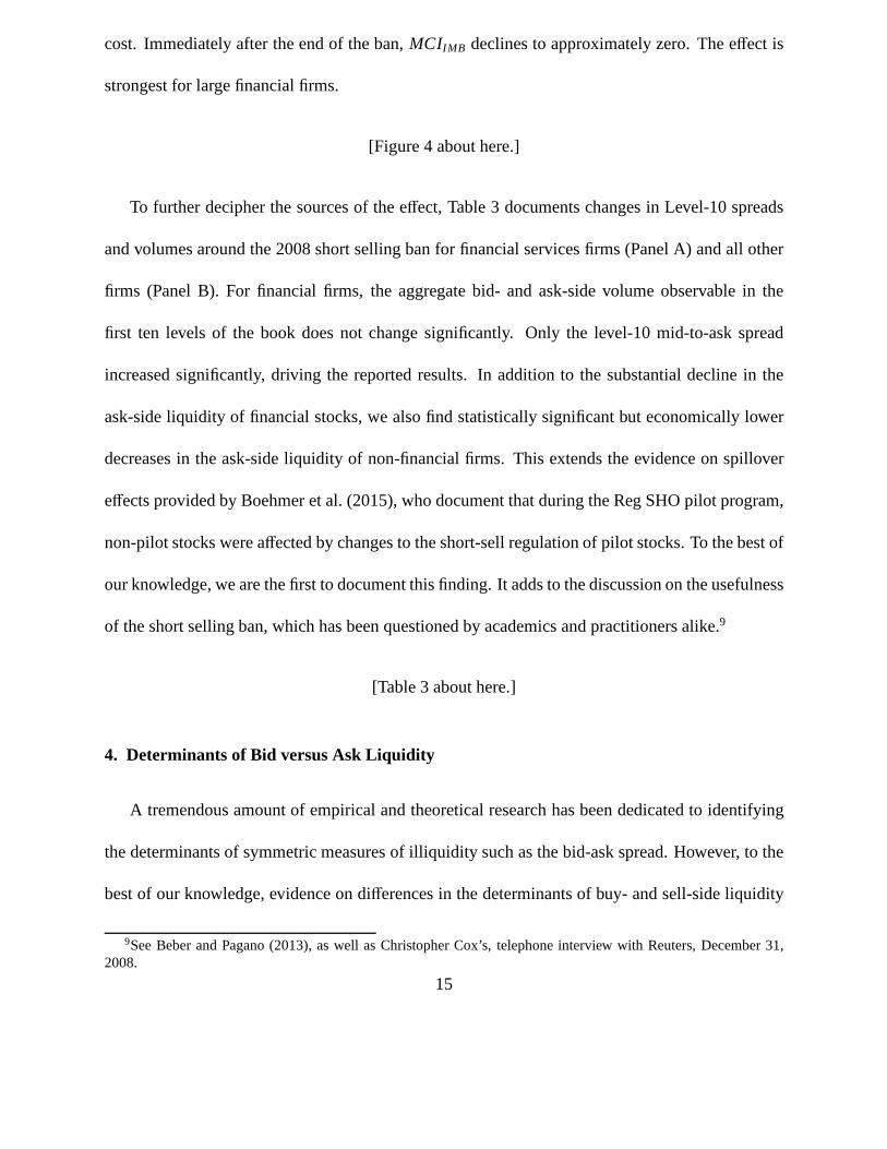
We observe improvements in market liquidity (decreases in transaction costs) prior to the fi-

nancial crisis. In relative terms, the decrease in transaction costs was larger for firms with a high

13

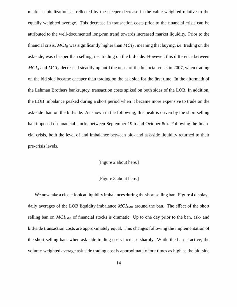
market capitalization, as reflected by the steeper decreasein the value-weighted relative to the

equally weighted average. This decrease in transaction costs prior to the financial crisis can be

attributed to the well-documented long-run trend towards increased market liquidity. Prior to the

financial crisis,MCIB was significantly higher thanMCIA, meaning that buying, i.e. trading on the

ask-side, was cheaper than selling, i.e. trading on the bid-side. However, this difference between

MCIA andMCIB decreased steadily up until the onset of the financial crisisin 2007, when trading

on the bid side became cheaper than trading on the ask side forthe first time. In the aftermath of

the Lehman Brothers bankruptcy, transaction costs spiked on both sides of the LOB. In addition,

the LOB imbalance peaked during a short period when it becamemore expensive to trade on the

ask-side than on the bid-side. As shown in the following, this peak is driven by the short selling

ban imposed on financial stocks between September 19th and October 8th. Following the finan-

cial crisis, both the level of and imbalance between bid- andask-side liquidity returned to their

pre-crisis levels.

[Figure 2 about here.]

[Figure 3 about here.]

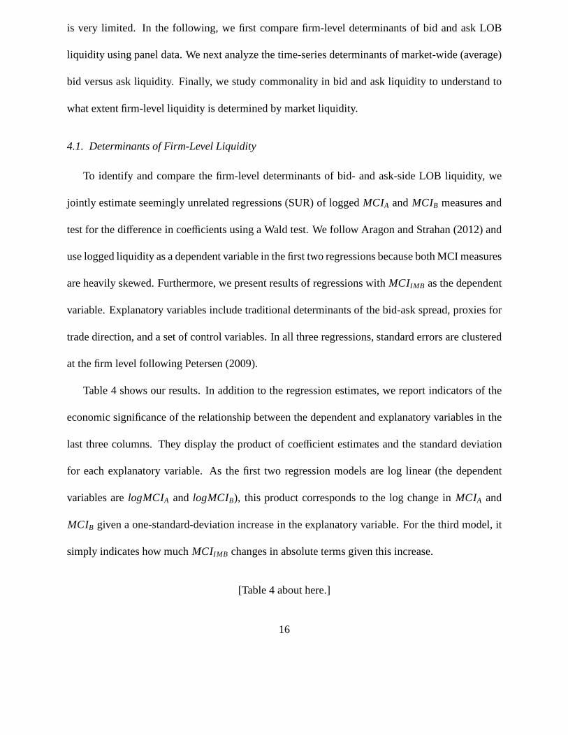
We now take a closer look at liquidity imbalances during the short selling ban. Figure 4 displays

daily averages of the LOB liquidity imbalanceMCIIMB around the ban. The effect of the short

selling ban onMCIIMB of financial stocks is dramatic. Up to one day prior to the ban,ask- and

bid-side transaction costs are approximately equal. This changes following the implementation of

the short selling ban, when ask-side trading costs increasesharply. While the ban is active, the

volume-weighted average ask-side trading cost is approximately four times as high as the bid-side

14

cost. Immediately after the end of the ban,MCIIMB declines to approximately zero. The effect is

strongest for large financial firms.

[Figure 4 about here.]

To further decipher the sources of the effect, Table 3 documents changes in Level-10 spreads

and volumes around the 2008 short selling ban for financial services firms (Panel A) and all other

firms (Panel B). For financial firms, the aggregate bid- and ask-side volume observable in the

first ten levels of the book does not change significantly. Only the level-10 mid-to-ask spread

increased significantly, driving the reported results. In addition to the substantial decline in the

ask-side liquidity of financial stocks, we also find statistically significant but economically lower

decreases in the ask-side liquidity of non-financial firms. This extends the evidence on spillover

effects provided by Boehmer et al. (2015), who document that during the Reg SHO pilot program,

non-pilot stocks were affected by changes to the short-sell regulation of pilot stocks. To the best of

our knowledge, we are the first to document this finding. It adds to the discussion on the usefulness

of the short selling ban, which has been questioned by academics and practitioners alike.9

[Table 3 about here.]

4. Determinants of Bid versus Ask Liquidity

A tremendous amount of empirical and theoretical research has been dedicated to identifying

the determinants of symmetric measures of illiquidity suchas the bid-ask spread. However, to the

best of our knowledge, evidence on differences in the determinants of buy- and sell-side liquidity

9See Beber and Pagano (2013), as well as Christopher Cox’s, telephone interview with Reuters, December 31,2008.

15

is very limited. In the following, we first compare firm-leveldeterminants of bid and ask LOB

liquidity using panel data. We next analyze the time-seriesdeterminants of market-wide (average)

bid versus ask liquidity. Finally, we study commonality in bid and ask liquidity to understand to

what extent firm-level liquidity is determined by market liquidity.

4.1. Determinants of Firm-Level Liquidity

To identify and compare the firm-level determinants of bid- and ask-side LOB liquidity, we

jointly estimate seemingly unrelated regressions (SUR) ofloggedMCIA andMCIB measures and

test for the difference in coefficients using a Wald test. We follow Aragon and Strahan (2012)and

use logged liquidity as a dependent variable in the first two regressions because both MCI measures

are heavily skewed. Furthermore, we present results of regressions withMCIIMB as the dependent

variable. Explanatory variables include traditional determinants of the bid-ask spread, proxies for

trade direction, and a set of control variables. In all threeregressions, standard errors are clustered

at the firm level following Petersen (2009).

Table 4 shows our results. In addition to the regression estimates, we report indicators of the

economic significance of the relationship between the dependent and explanatory variables in the

last three columns. They display the product of coefficient estimates and the standard deviation

for each explanatory variable. As the first two regression models are log linear (the dependent

variables arelogMCIA and logMCIB), this product corresponds to the log change inMCIA and

MCIB given a one-standard-deviation increase in the explanatory variable. For the third model, it

simply indicates how muchMCIIMB changes in absolute terms given this increase.

[Table 4 about here.]

16

Our MCI measures capture the cost of trading in the LOB, whichconsists of a series of bid-

ask quotes. It is thus natural to regressMCIA and MCIB on the traditional determinants of the

bid-ask spread. These include a market maker’s order processing costs, his inventory holding

costs (Garman (1976), Stoll (1978), Amihud and Mendelson (1986), Ho and Stoll (1981)) and his

costs of adverse selection due to the risk of being picked off by an informed trader (Glosten and

Milgrom (1985), Kyle (1985)). In addition, several studies, including Chacko et al. (2008), argue

that market makers can use their power to extract rents from selling immediacy if market making

is not perfectly competitive. We proxy for these four determinants as follows.10

We measure order processing costs asTurnover, defined as the log of the daily dollar trading

volume reported in CRSP. Not surprisingly, the relationship betweenTurnoverand our illiquidity

measureslogMCIA andlogMCIB is negative and highly significant. Furthermore,Turnoverhas by

far the highest economic impact on trading costs. A one-standard-deviation decrease inTurnover

results in an increase (stated as log change) of 97.9% (101.9%) in MCIA (MCIB). More impor-

tantly, the impact ofTurnoveris higher on bid-side liquidity than on ask-side liquidity,which is

also reflected by a positive and significant relationship betweenTurnoverandMCIIMB.

Our proxy for inventory holding costs is realized volatility, RealizedVol, which we compute

from intraday TAQ data. In line with expectations, the relationship between both of our illquidity

measures andRealizedVolis positive, statistically significant and economically meaningful. A

one-standard-deviation increase in volatility increasesMCIA and MCIB by approximately 42%.

RealizedVoldoes not appear to drive difference in bid- versus ask-side liquidity; the difference

between coefficients is insignificant. The relationship between realizedvolatility and MCIIMB is

10For an overview of empirical analyses of the bid-ask spread using these and alternative proxies, see Bollen et al.(2004).

17

negative but only significant at the 10% level.

Given the lack of more detailed information, we captureCompetitionbetween market makers

as one minus the Herfindahl index measuring the dispersion oftrading volume across exchanges

based on TAQ data. We find a statistically and economically significant negative relationship be-

tweenCompetitionand trading costs. We further observe that its impact on bid-side liquidity is

substantially higher than that on ask-side liquidity together with a positive and statistically signif-

icant coefficient in theMCIIMB regression. A potential explanation is that market makers are able

to extract higher rents from the demand for immediacy on the sell (bid) side because the need to

sell shares quickly is arguably more widespread than the urge to buy them. Increased competition

would then reduce the liquidity provider’s rent more on the bid than on the ask side.

Finally, we include the Easley et al. (1996) probability of informed trading (PIN) and absolute

order imbalance (AbsOrderImbalance) as proxies for the cost of adverse selection.11 Again in line

with expectations, we find thatMCI increases in adverse selection costs. Absolute order imbalance

has significantly stronger effect on bid- than ask-side transaction costs, while the same cannot be

said aboutPIN. However, we should note the economic importance of these factors is relatively

low.

Our next set of variables labelled “Trade Direction” captures whether a stock is or has been un-

der directional trading pressure. It includes contemporaneous order imbalance (OrderImbalance)

and return (Ret), the previous day’s return (RetLag), as well as the Campbell et al. (2008) long-run

excess return until the day before (ExretAvg).

11The calculation ofPIN is based on the approach described in Lin and Ke (2011) and detailed in Appendix A-5.We compute order imbalance as the difference between the number of Lee and Ready (1991) buy minus sell ordersscaled by their sum. We include the daily availableAbsOrderImbalancein addition toPIN, as the latter needs to beestimated from longer time series – we use data from the preceding month.

18

All these measures exhibit a significantly negative relationship with logMCIA and a signifi-

cantly positive relationship withlogMCIB and are, in economic terms, the most important determi-

nants of imbalance in LOB liquidity,MCIIMB. Higher lagged/contemporaneous returns or buy-sell

order imbalance implies a higher ask-side liquidity and a lower bid-side liquidity. Loosely speak-

ing, investors provide more bid and less ask side liquidity during or following falling stock prices,

while the opposite holds when stock prices rise. This in turnsuggests that liquidity providers

exhibit contrarian behavior. Our findings are also in line with the model of Rosu (2009), which

predicts that a sell order will decrease bid prices more thanask prices.

Finally, our set of control variables includes logged market capitalization (S ize), the Camp-

bell et al. (2008) measures log stock price winsorized at $15, market to book ratio (MB), leverage

(Lever), profitability (Pro f it), and cash holdings (Cash), a dummy for financial services firms

(FS), one for days during which the 2008 short selling ban wasactive (Ban), and their interac-

tion. Liquidity increases inS ize, which is the second most important determinant oflogMCIA

and logMCIB in economic terms. More importantly, this effect is not only statistically but also

economically stronger for ask-side than bid-side liquidity. It is also noteworthy that the illiquidity

of non-financial services firms decreased during the 2008 short selling ban, indicated by theBan

coefficient. For financial stocks, this increase was stronger on the ask than on the bid side. These

findings suggest that effects from the short selling ban on financial stocks spilled over to unregu-

lated non-financial stocks. They are in line with the evidence for illiquidity spillovers in regulatory

experiments documented in Boehmer et al. (2015). The coefficients of most other controls are not

surprising and some of them have statistically different effects on bid and ask side liquidity, but

they do not seem to be economically important.

19

4.2. Time-Series Determinants of Aggregate Liquidity

In this section, we examine whether the differences between firm-level determinants of bid-

and ask-side liquidity persist at the market-level. As documented in Table 5, we regress the daily

time series of equally and value-weighted averages ofMCIA, MCIB andMCIIMB on independent

variables comprising those used by Brennan et al. (2012) to analyze the time series of their monthly

buy- and sell-side measures of liquidity. Their variables include the VIX implied volatility index12

(VIX), the ratio of the number of stocks with a positive contemporaneous return to that with a

negative return (UpDown Ratio), today’s and yesterday’s market return (RetM andRetMLag), as

well as the TED spread measuring funding liquidity (TED). We add the log of the market-wide

dollar trading volume measured in billions of USD (TurnoverM), as turnover is the most important

determinant of LOB liquidity at the firm level, and a dummy variable for the 2008 short selling

ban on financial stocks (Ban). Market returns and volume are computed from stocks listedon the

NYSE, AMEX and NASDAQ.

As in the previous section, we assign these variables to the categories “Traditional Determi-

nants”, “Trade Direction”, and “Control Variables”. As opposed to firm-levelMCI measures,

their averages are not plagued by heavy skewness, and we therefore do not estimate log-linear re-

gressions but use the non-transformedMCI measures as dependent variables. As in the previous

section, we report indicators of the economic significance of the relationship between dependent

and explanatory variables, which are displayed in Panel B ofTable 5. It reports the product of

coefficient estimates and the standard deviation for each explanatory variable. In contrast to the

12Whaley (2008) argues that the VIX implied volatility index is asymmetric by construction, with a greater responseto downward price movements than upward price movements. Inother words, VIX is more volatile in down thanup markets. This fact in turn might affect the interpretation of the coefficient estimate on this variable, which willbe smaller in down markets compared to up markets, ceteris paribus. To mitigate this effect, we also consideredalternative measures of market volatility, such as realized volatility computed using daily market returns. Our resultsremain quantitatively similar to those presented.

20

previous section, none of our dependent variable is logged.These statistics thus indicate how

much the dependent variable changes in absolute terms givena one-standard-deviation increase in

the explanatory variable.

[Table 5 about here.]

Our findings indicate that the macro equivalents to our most important determinants of firm-

level MCI measures are indeed important determinants of aggregate LOB liquidity and imbalance.

Again, turnover (TurnoverM) and volatility (VIX) drive aggregate LOB liquidity. Their relation-

ship with equally and value-weightedMCIA andMCIB is statistically highly significant. In addi-

tion, they are the two most economically important determinants of LOB liquidity. The impact of

TurnoverM on both equally and value-weighted bid side liquidityMCIB is substantially more neg-

ative than onMCIA. Results for the relationship between measures of trade direction, including

contemporaneous returns, lagged returns, and theUpDown Ratio, are mixed. Their relationship

with MCIA andMCIB varies across regression specifications, and even statistically significant re-

lationships are of low economic importance. However, consistent with our firm-level results, their

impact onMCIB is higher than that onMCIA and all of them are negatively related to equally and

value-weighted LOB imbalanceMCIIMB. When markets rise, bid-side liquidity deteriorates more

(or improves less) than ask-side liquidity. This indicatesthat the previously documented contrarian

behavior of liquidity providers at the firm-level carries over to the aggregate market.

Surprisingly, while (not reported) bivariate correlations between the TED spread and allMCI

measures are positive, the relationship becomes negative after controlling for other factors in three

out of four regression specifications. For our dataset and atan aggregate level, we can therefore not

confirm the hypothesis that limited funding liquidity during the financial crisis drove transaction21

costs, as would be expected from Brunnermeier and Pedersen (2009), for instance. The differential

impact of the 2008 short selling ban on bid versus ask liquidity displayed in Figure 4 remains

significant in this multivariate setting, as indicated by the significant difference between theBan

coefficients and the positive and significant relationship between BanandMCIIMB.

Overall, our results on the relationship between trading costs and explanatory variables are

in line with our expectations based on the predictions of microstructure models and the study

of aggregate market liquidity by Chordia et al. (2001). However, neither the theoretical nor the

empirical literature provides much guidance on whether theexplanatory variables should have any

differential relationship with the ask and bid sides. The only exception is Brennan et al. (2012),

who analyze differences in the determinants of monthly Level I estimates of buy- and sell-side

liquidity. Our results on the time-series determinants of aggregate liquidity complement theirs in

that they are based on daily Level II data comprising the financial crisis, confirm the differential

impact of the 2008 short selling ban on bid versus ask liquidity, and highlight the substantial

economic impact ofTurnoverM andVIX on liquidity. As volatility, turnover, and returns drive

LOB liquidity both at the firm and aggregate levels, a naturalnext step is to examine the prevalence

of commonality in liquidity.

4.3. Commonalities in Bid and Ask Side Liquidity

As Korajczyk and Sadka (2008) note, the absolute level of illiquidity only requires a small

premium to compensate investors for higher transaction costs. In contrast, systematic comove-

ments of individual with market-wide liquidity can justifysubstantial liquidity premia. Accord-

ingly, commonality in market liquidity has important implications for asset pricing. In this section,

we document differences in bid- versus ask-side commonality and by studyingits time variation

22

around the financial crisis.13

4.3.1. Estimation

Commonality in LOB liquidity implies covariation between stock-specific and aggregateMCI

measures. As in Chordia et al. (2000), we estimate the following market model of liquidity for

each stock:

∆LIQi,t = αi + β1,i∆LIQM\i,t + β2,i∆LIQM\i,t−1 + β3,i∆LIQM\i,t+1 + βX,iX t + εi,t, (7)

where∆LIQi,t is the percentage change in stock i’s liquidityLIQ from trading day t-1 to t and

∆LIQM\i,t the contemporaneous change in the cross-sectional averageof LIQ. X t represents con-

trol variables including lagged, contemporaneous and leadmarket returns, as well as the relative

change in the realized volatility of stocki. Studying changes rather than levels reduces econo-

metric problems due to the persistence of liquidity. When computing average market liquidity

LIQM \ i, we exclude stocki. This avoids an overestimation of commonality due to noisy data and

outliers. As highlighted by Chordia et al. (2000), althoughthis adjustment has a minor effect on

the explanatory variables and thus the coefficient for each stock, it can substantially affect average

betas.

4.3.2. Commonality in the Pooled Sample

Table 6 presents the results of stock-level regressions using data from the entire sample period.

Commonality is documented for bid- and ask-side LOB liquidity and its imbalance. In line with

Chordia et al. (2000), the results confirm the existence of commonality in bothMCIA andMCIB.

13Studies documenting and explaining different features of commonality include Chordia et al. (2000), Coughenourand Saad (2004), Korajczyk and Sadka (2008), Kamara et al. (2008), Comerton-Forde et al. (2010), and Karolyi et al.(2012).

23

The sum of concurrent, lead and lag coefficients is positive and significant, and market liquidity

contributes 1.6% (1.5%) to the explanatory power ofMCIB (MCIA) regressions on average. While

this difference in marginal explanatory power∆R2 is insignificant, the economic magnitude of

commonality is significantly larger on the bid than on the askside. The sum of the three market

illiquidity coefficients equals 0.62 for the former and 0.54 for the latter. A potential explanation

for this is that market participants’ need to sell is likely to co-move more systematically than their

need to buy, especially in times of economic distress. Market sells (which are matched with and

thus eliminate limit buy orders) are then likely to co-vary more systematically than market buys.

Similarly, the number of placed limit buy (bid) orders is then likely to decrease in a more systematic

fashion than is true for limit sells. To further investigatethis hypothesis, the next section examines

changes in the level of commonality around the financial crisis.

Liquidity imbalancesMCIIMB show no signs of commonality. On average, none of the three

coefficients is significant. The median∆R2 is zero. This indicates that the strong positive rela-

tionship betweenMCIIMB and stock returns documented in Section 5 is not due to the pricing of a

systematic liquidity factor but rather reflects temporary and idiosyncratic price pressure.

[Table 6 about here.]

4.3.3. Time Series of Commonality

In this section, we explore differences in the variations of ask- and bid-side liquidity common-

ality over time. Given the lack of commonality inMCIIMB, we do not report time series results for

this variable but instead focus onMCIA andMCIB. Table 7 presents the results of the stock-level

regressions described above estimated using data from non-overlapping six-month sample periods

instead of the full sample period. Each row in Table 7 shows averages and statistics from a t-test24

for the sum of all three market liquidity coefficients (Sum), together with average∆R2. During the

2008 financial crisis, LOB liquidity of firms in the financial services industry was affected by fac-

tors less relevant for industrial firms, including the shortselling ban on financial stocks discussed

in Section 3. We therefore report commonality results for the subsample of financial services firms

(SIC codes 6000-6999) and industrial firms (all others) separately.

[Table 7 about here.]

We find substantial time variation in liquidity commonality. Commonality increases for both

industrial and financial services firms on the bid and ask sideduring the financial crisis, peaking

in the second half of 2008. In line with our hypothesis statedin the previous section,∆R2s are

significantly higher on the bid than on the ask side. Our results indicate that bid-side liquidity

is more prone to being driven by systematic factors in times of crisis than is ask-side liquidity.

This finding can explain why the premium for sell-side liquidity is higher than that for buy-side

liquidity, as reported by Brennan et al. (2012) and Brennan et al. (2013). In contrast to the peak

of commonality at the core of the financial crisis at the end of2008, the substantial increase in

commonality in the second half of 2009 is puzzling, and we leave it to future research to identify

its causes.

5. Predictive Power of Bid versus Ask Liquidity

In this section, we analyze the differences in the power of ask- and bid-side liquidity in predict-

ing stock returns. We first make predictions concerning the channels through which we expect ask-

and bid-side liquidity to affect returns and then test our hypotheses in-sample and out-of-sample

through portfolio sorts.

25

5.1. Two Channels for Return Predictability

There are two known channels through which LOB liquidity canaffect returns. First, Cao et al.

(2009) and Brogaard et al. (2014) argue that an imbalance between sell- and buy-side liquidity can

result in short-term price pressure and document a positiverelationship between Level I order im-

balance and next-day stock returns. Translating their finding to the LOB, short-run returns should

be high when the bid side is more liquid than the ask side (MCIB < MCIA). Second, the existence

of a liquidity premium documented in numerous studies including Amihud and Mendelson (1986),

Brennan and Subrahmanyam (1996), and Amihud (2002) impliesthat long-run returns increase in

both laggedMCIA andMCIB.

Taken together, we expect the following. The first channel implies a positive relationship be-

tween imbalance (MCIIMB) and returns, which is more pronounced for daily than for monthly

returns. Both channels imply a positive relationship between ask illiquidity (MCIA) and both daily

and monthly returns. In contrast, the relationship betweenMCIB and returns is less straightforward

to predict.

We expect the liquidity premium to result in a positive relation between laggedMCIB and

returns (second channel). In contrast, as a high bid-side liquidity (a low MCIB) reflects a high

demand for a stock, upside price pressure can result in a negative relation between laggedMCIB

and returns (first channel). As price pressure is typically short lived, we expect to observe a more

positive relation betweenMCIB and returns on a monthly basis (where the second channel domi-

nates) than on a daily basis (where both channels can offset each other). To test these predictions,

we report results for in-sample predictive regressions of daily and monthly returns on our three

MCI measures, as well as for daily and monthly portfolio sorts.

We expect the liquidity premium to result in a positive relationship between laggedMCIB and26

monthly returns and the relationship betweenMCIB and next-day returns to be less positive than

for MCIA. To test these predictions, we report results for in-samplepredictive regressions of daily

and monthly returns on our threeMCI measures, as well as for daily and monthly portfolio sorts.

5.2. In-Sample Predictability

We first estimate linear regressions for the pooled sample. Specifically, we regress daily or

monthly return on lagged values ofMCIA, MCIB or MCIIMB and control for lagged returns in

each regression. Table 9 presents coefficient estimates and HAC standard errors. The left side

displays the power of bid- versus ask-side liquidity in forecasting daily returns. In line with our

expectations, daily returns increase in laggedMCIIMB andMCIA and less so inMCIB. Signs and

levels of significance are identical in regressions with monthly returns, displayed on the right side

of the table. However, theMCIB coefficient is no longer lower than theMCIA coefficient, which is

consistent with the prediction that the liquidity premia channel dominates at longer horizons.

[Table 8 about here.]

We complement the in-sample results for the pooled sample with firm-by-firm predictive re-

gressions that include the same variables as before. We require a stock to have at least 24 monthly

or 63 daily observations to be included in this analysis. Figure 5 presents the (winsorized) distribu-

tion of the coefficient estimates on theMCI measures from the firm-by-firm predictive regressions.

We complement the histogram with the descriptive statistics of the (unwinsorized) distribution in

Table 9.

Overall, coefficient signs and significances are similar to those found for the pooled sample.14

At the daily level, an increase in bothMCIA and MCIB predicts, on average, higher returns. In

14The adjusted R2 of the firm-by-firm regressions are very low and are not reported for brevity. This is not surprising,as it is well known that stock returns are notoriously difficult to forecast.

27

line with our expectations, the evidence is stronger forMCIA, which has a positive and significant

coefficient estimate for 25% of the stocks in our sample, compared with 14% for MCIB. This is

also reflected in the coefficient estimates on laggedMCIIMB, which, on average, positively predicts

daily returns. At the monthly level, results are similar forthe predictive relationship between

and returns andMCIA as well asMCIB. However, the predictive relationship betweenMCIIMB

and monthly returns is less clear at the firm level. The coefficient estimates on laggedMCIIMB

are almost symmetrically distributed around zero, with almost an equal number of positive and

negative coefficient estimates and only approximately 8% that are significant. This suggests that

MCIIMB does not possess much predictive power at longer horizons and is consistent with the

prediction that the liquidity premia channel dominates at longer horizons.

[Figure 5 about here.]

[Table 9 about here.]

5.3. Portfolio Sorts

Finally, we verify the robustness of the in-sample evidenceby conducting portfolio sorts. Ta-

ble 10 reports equally and value-weighted returns (Panel A)and four-factor alphas (Panel B) of

portfolios formed on a daily basis. At the end of each tradingday, stocks are assigned to a portfo-

lio according to the quintile of theirMCI measure and held until the end of the next trading day,

when new portfolios are defined. Of course, these portfolio strategies are very costly to implement

given the ongoing rebalancing. Our results therefore do notindicate whether a strategy is profitable

after trading costs. Rows 1-5 report returns and alphas of the respective portfolio. For alphas, re-

ported in Panel B, we also display the level of significance totest whether they are different from

zero. We omit the results of these tests in Panel A, as all portfolio returns are significantly positive.28

Table 11 reports the same results but for portfolios formed at the end of month M (depending on

the averageMCI value in M) and held until the end of month M+1.

[Table 10 about here.]

[Table 11 about here.]

Our results strongly support our initially stated hypotheses. Equally weighted daily returns and

alphas increase significantly inMCIA andMCIIMB but not inMCIB. Over one year (252 trading

days), the return on the equally weighted highMCIIMB portfolio is 21.17% higher than that of the

low MCIIMB portfolio. In fact, the four-factor alpha of the latter is negative, indicating that there is

both upward and downward price pressure. The highMCIIMB quintile alpha of 5.948 basis points

per day is substantial. However, entering a long position inhigh MCIIMB implies buying stocks

with an illiquid ask (sell) side, which is particularly costly. Comparing equally weighted to value-

weighted results, the price pressure hypothesis only appears to hold for smaller stocks. The return

and alpha of the high value-weightedMCIIMB portfolio do not differ significantly from those of the

low MCIIMB portfolio. This is not true forMCIA, which may be because it also captures the second

channel through which liquidity affects returns, liquidity premia. These become more visible in

monthly portfolio sorts. In line with our hypothesis, returns and alphas increase in bothMCIA

andMCIB. While the difference between high and lowMCI is not statistically significant, this is

likely due to the relatively low number of months covered by our sample, which limits the power

of this monthly analysis. In sum, our results are in line withthe argument that lagged liquidity

can affect short-run returns by creating price pressure and is positively related to long-run return

because investors demand a premium for holding illiquid stocks.

29

6. Conclusion

In this paper, we disentangle buy- and sell-side liquidity at daily frequency by observing (rather

than estimating) ask- and bid-side transaction costs in eleven years of comprehensive, high fre-

quency limit order book (LOB) data. Observing the precise dynamics of bid- and ask-side liquidity

at daily frequency enables us to conduct novel analyses of their determinants, commonalities, and

pricing in the cross section that contribute to existing research in multiple ways.

First, average bid- and ask-side transaction costs are, respectively, 1.64 and 1.54 basis points

per additional one thousand USD traded, suggesting that selling is, on average, more expensive

than buying. Second, the ask- but not bid-side liquidity of financial stocks deteriorates during the

2008 short selling ban. Third, the factors driving liquidity differ between bid- and ask-side. Both

at the firm- and at the market-level, well-known determinants of the bid-ask spread have a stronger

impact on bid- than ask-side transaction costs. Furthermore, we document that bid-side (ask-

side) liquidity decreases (increases) in lagged short- andlong-term returns, indicating persistent

contrarian behavior in limit orders. Fourth, liquidity commonality increases during the financial

crisis, more so on the bid than on the ask side. Finally, ask- but not bid-side liquidity predicts daily

returns, while both forecast monthly returns.

The relevance of our results extends beyond academic research. Our analysis of changes in

bid- and ask-side liquidity around the 2008 short selling ban can helppolicy makersunderstand

the mechanisms through which regulatory interventions affect liquidity provision. Amongst others,

we document that the ban’s asymmetric effect on liquidity provision was not limited to financial

stocks but extended to industrial stocks, indicating spillover effects. Our study can helpinvestors

understand when differentiating between ask- and bid-side liquidity matters. At times, it can be

30

cheap to buy but expensive to sell and vice versa. Strategiesintended to reduce transaction costs

should depend on the trade direction. Furthermore, we document that LOB imbalances reflect price

pressure and can predict daily returns, while the predictive power of LOB liquidity for monthly

returns appears to be driven by liquidity premia.

Our results indicate directions for future research using limit order book data. For instance, it

would be interesting to further examine the impact of regulatory intervention on liquidity provision

by studying the effect of Regulation SHO on the LOB. Comparing the LOBs of NASDAQand

NYSE can provide insights into the relevance of differences in trading mechanisms on liquidity.

Finally, future research could explore whether information in the LOB can be used to predict the

higher moments of the return distribution.

31

Appendix

A-1. Matching TRTH and CRSP

The primary security identifier in the TRTH data is the Reuters Instrument Code (RIC), which

consists of a security’s ticker symbol and an optional extension indicating specific exchanges or

security types. The primary identifier of a security in the CRSP database is its Permno. The only

additional identifier in our TRTH dataset is the company name. As tickers and company names vary

over time and across databases, they are known to be unreliable identifiers for matching databases.

We therefore establish a table allowing us to link TRTH and CRSP data on a daily basis using

three matching criteria: the level of closing prices, the correlation between closing price returns

and similarities in the ticker or company name. In sum, we consider the criteria to be strict and,

accordingly, the resulting link to be conservative. Despite the strictness of the link, we nevertheless

cover more than 98% of the volume in NYSE common stocks included in the CRSP database. The

following describes the matching procedure in greater detail.

In a first step, we identify the CRSP security that best matches the price patterns of a TRTH

security in a given month from the entire universe of NYSE-listed securities reported in CRSP for

each TRTH stock-month. To do so, we need daily time series of closing prices. While a CRSP

closing price is typically the last transaction price, we derive the TRTH closing price as the Level-1

midprice of the last book snapshot reported for a stock during trading hours. We then gather the

time series of daily closing prices reported in TRTH and CRSPinto monthly blocks. Stock-months

with fewer than 10 prices are excluded from the matching procedure at this stage. Links for such

stock-months with very few observations are established using the links obtained from the months

around them in a later step.

32

We now compute two matching parameters, price distance and return correlation. The former is

the average absolute difference between the time series of prices for a given stock in agiven month.

The second is the correlation between returns computed fromthe prices. If, in a given month, the

CRSP security with the highest correlation is also the one with the lowest price distance, we save

the CRSP Permno identifier together with the value of both matching parameters. If this is not

the case, but the CRSP stock with the highest correlation with the TRTH stock in a given month

has an average price distance of less than l%, we use this as the best match and again save both

parameters. If no best match has been identified yet and the correlation computed for the security

with the lowest price distance is at least 90%, we use the minimum-distance security as the best

match.

This step produced a matrix containing a Permno for each RIC-month for which a best match

was identified. We observe very few outliers in these Permno time series, indicating the valid-

ity of the employed matching criteria. We replace these outliers with the Permno link from the

surrounding months.

In a next step, we validate the monthly link by comparing the RIC identifier – which contains

the security’s ticker symbol – to all CRSP tickers reported in the CRSP names file for a given

Permno. If we find a CRSP ticker symbol that fully matches the RIC ticker or only differs by one-

or two-digit ticker extensions included in the RIC, we consider a link valid. For all non-verified

links, we manually compare the company names from CRSP and TRTH. If these are not identical,

we discard the link. Out of 6959 TRTH securities for which we identify a link in at least one

month, only 14 are not verified based on ticker or company name.

Finally, we translate the monthly linking table to a daily one to avoid losing data from stock-

months with fewer than 10 price observations. In a month without a link, we use the link from the33

preceding or subsequent month.15 We then identify the beginning (ending) day of a link as the first

(last) one with a price distance of less than 5%.

A-2. Sample Selection

Securities in the TRTH database are identified by the ReutersInstrument Code (RIC). Between

2002 and May 2006, the MD database includes RICs ending with “.CX”, <.CX> denoting Nas-

daq’s Computer-Assisted Execution System (CAES). According to Thomson Reuters, the CAES

quote is the best aggregated quote from market makers participating in the Intermarket Trading

System (ITS). We compared data entries between securities with RICs ending in .CX to their coun-

terpart not ending in .CX for randomly selected dates and found that the data are fully identical.

We therefore exclude all securities with RICs with a .CX ending.

After the exclusion of these double entries, our initial dataset includes 52.44 billion snapshots.

We require each snapshot to give a full picture of the book, excluding any snapshot for which

order price or volume data are missing for any level of the book. This reduces the number of

snapshots to 49.61 billion. We next limit the sample to snapshots for which prices are strictly

monotonically increasing over the 20 levels of the book. This eliminates all negative bid-ask

spreads and decreases the sample size to 44.83 billion snapshots. In line with Korajczyk and Sadka

(2008), we delete entries with very large bid-ask spreads and those not reported for NYSE trading

hours.16 We then delete observations with a midprice of $1 or less or $1000 or more, yielding

44.49 billion observations. Limiting our sample to securities for which we are able to establish a

link to data reported in the CRSP files as detailed in AppendixA-1 further decreases this number

15This never causes a conflict because there are no occurrencesof stock-months without link that are preceded by alink that is different from the subsequent link.

16We delete observations with a Level-1 (10) ask price that is more than 25% (250%) higher than the Level-1 (10)bid price.

34

to 42.83 billion. Removing all securities other than ordinary common shares identified by a CRSP

sharecode of 10 or 11 results in our sample of 31.32 billion LOB snapshots. Finally, deleting all

firm-days with fewer than 100 snapshots in the TRTH data or fewer than 100 trades in the matched

TAQ dataset as well as observations without return data in CRSP or balance sheet information in

Compustat results in a sample of 31.19 billion observationsreported for 2,103 stocks over 2,740

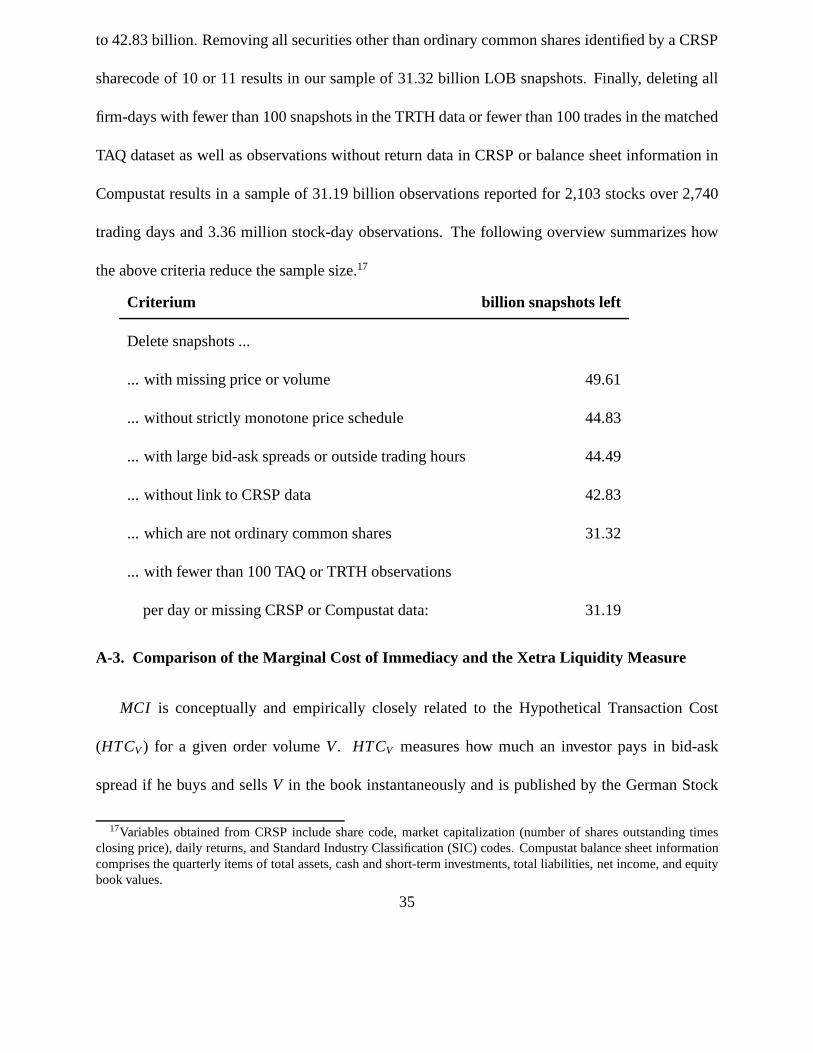
trading days and 3.36 million stock-day observations. The following overview summarizes how

the above criteria reduce the sample size.17

Criterium billion snapshots left

Delete snapshots ...

... with missing price or volume 49.61

... without strictly monotone price schedule 44.83

... with large bid-ask spreads or outside trading hours 44.49

... without link to CRSP data 42.83

... which are not ordinary common shares 31.32

... with fewer than 100 TAQ or TRTH observations

per day or missing CRSP or Compustat data: 31.19

A-3. Comparison of the Marginal Cost of Immediacy and the Xetra Liquidity Measure

MCI is conceptually and empirically closely related to the Hypothetical Transaction Cost

(HTCV) for a given order volumeV. HTCV measures how much an investor pays in bid-ask

spread if he buys and sellsV in the book instantaneously and is published by the German Stock

17Variables obtained from CRSP include share code, market capitalization (number of shares outstanding timesclosing price), daily returns, and Standard Industry Classification (SIC) codes. Compustat balance sheet informationcomprises the quarterly items of total assets, cash and short-term investments, total liabilities, net income, and equitybook values.

35

Exchange under the label “Xetra Liquidity Measure” to describe the LOB liquidity of traded secu-

rities.18 In Figure 1, theHTCV=US D 1mio corresponds to the length of the horizontal line and equals

approximately 5.5 basis points. Relative toHTCV, MCI has two main advantages. First,MCI ex-

hausts all information from the book, whileHTCV only uses information up to the level at which

the cumulative volume reachesV.19 Second,MCI can be calculated for any stock, whileHTCV is

restricted to LOBs with a cumulative bid and ask volume of at leastV. This makesHTC unsuit-

able for studying a wide cross-section of stocks. Although we accordingly do not report results

for HTC, we observe that in a given size category (allowing theHTC measure to be meaningful

across all stocks),HTCV andMCI are almost perfectly correlated.

We aggregate all TRTH measures on a daily basis by computing their equally weighted average.

To avoid spurious results due to extreme outliers, we winsorize all Level I and Level II variables

by setting the value below the 0.1 fractile (above the 99.9thpercentile) equal to the value of the 0.1

(99.9) fractile.

A-4. Calculation of Level I Measures

The following details the calculation of Level 1 measures ofliquidity computed from TAQ data.

The first set of level I liquidity measures is based on Holden and Jacobsen (2014). The authors

compare the quality of a wide range of liquidity measures constructed from the expensive Daily

TAQ (DTAQ) database to measures based on the more commonly used Monthly TAQ (MTAQ)

database. While they conclude that DTAQ is the first best, they suggest an interpolated time tech-

nique that makes it possible to improve the quality of MTAQ measures. We use these improved

18See Roesch and Kaserer (2014).19In the example given in Figure 1, the measure ignores the information contained in levels 7-10 of the ask schedule.

36

MTAQ measures as a benchmark to assess the marginal information content of our Level II mea-

sures. Given the substantial correlation between some of their measures, we report results only

for the following measures. Whenever necessary, we use the Lee and Ready (1991) algorithm to

classify orders into buys and sells.

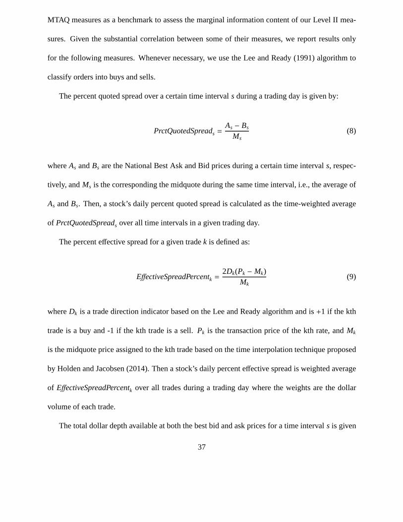
The percent quoted spread over a certain time intervals during a trading day is given by:

PrctQuotedSpreads =As − Bs

Ms(8)

whereAs andBs are the National Best Ask and Bid prices during a certain timeintervals, respec-

tively, andMs is the corresponding the midquote during the same time interval, i.e., the average of

As andBs. Then, a stock’s daily percent quoted spread is calculated as the time-weighted average

of PrctQuotedSpreads over all time intervals in a given trading day.

The percent effective spread for a given tradek is defined as:

EffectiveSpreadPercentk =2Dk(Pk − Mk)

Mk(9)

whereDk is a trade direction indicator based on the Lee and Ready algorithm and is+1 if the kth

trade is a buy and -1 if the kth trade is a sell.Pk is the transaction price of the kth rate, andMk

is the midquote price assigned to the kth trade based on the time interpolation technique proposed

by Holden and Jacobsen (2014). Then a stock’s daily percent effective spread is weighted average

of EffectiveSpreadPercentk over all trades during a trading day where the weights are thedollar

volume of each trade.

The total dollar depth available at both the best bid and ask prices for a time intervals is given

37

by :

TotalDepthDollars = Bs× QBs + As× QA

s (10)

whereQAs andQB

s are the total quantities available at the best ask and bid quotes, respectively. A

stock’s daily total dollar depth can then be calculated as the time-weighted average of total dollar

depth available over all time intervals. The total dollar depth imbalance between bid and ask sides

is defined as the time-weighted average of the ratio of dollardepth available at the best ask price

to total dollar depth available at both the best bid and ask prices.

The percent price impact for the kth trade is given by:

PercentPriceImpactk =2Dk(Mk+5 − Mk)

Mk(11)

whereMk+5 is the midquote price five minutes after the kth trade. The percent price impact for

a stock in a given trading is the dollar-volume-weighted average of percent price impact over all

trades.

We include two different measures of imbalance against which we can benchmark our principal

measure of imbalanceMCIIMB. Similar to Holden and Jacobsen (2014), we compute a measureof

order imbalance as:

OrderImbalance=NB − NS

NB + NS, (12)

whereNB andNS are the number of buys and sells according to the Lee and Ready(1991) trade

classification. In addition, we calculate the Level 1 quantity imbalance as:

TotalDepthDollarImbalance=As × QA

s

Bs× QBs + As × QA

s

, (13)

38

where the denominator corresponds to Equation 10.

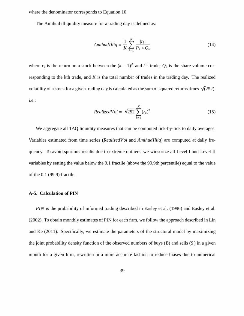
The Amihud illiquidity measure for a trading day is defined as:

AmihudIlliq=1K

K∑

k=1

|rk|Pk ∗ Qk

(14)

whererk is the return on a stock between the (k − 1)th andkth trade,Qk is the share volume cor-

responding to the kth trade, andK is the total number of trades in the trading day. The realized

volatility of a stock for a given trading day is calculated asthe sum of squared returns times√

(252),

i.e.:

RealizedVol=√

252K

∑

k=1

(rk)2 (15)

We aggregate all TAQ liquidity measures that can be computedtick-by-tick to daily averages.

Variables estimated from time series (RealizedVoland AmihudIlliq) are computed at daily fre-

quency. To avoid spurious results due to extreme outliers, we winsorize all Level I and Level II

variables by setting the value below the 0.1 fractile (abovethe 99.9th percentile) equal to the value

of the 0.1 (99.9) fractile.

A-5. Calculation of PIN

PIN is the probability of informed trading described in Easley et al. (1996) and Easley et al.

(2002). To obtain monthly estimates of PIN for each firm, we follow the approach described in Lin

and Ke (2011). Specifically, we estimate the parameters of the structural model by maximizing

the joint probability density function of the observed numbers of buys (B) and sells (S) in a given

month for a given firm, rewritten in a more accurate fashion toreduce biases due to numerical

39

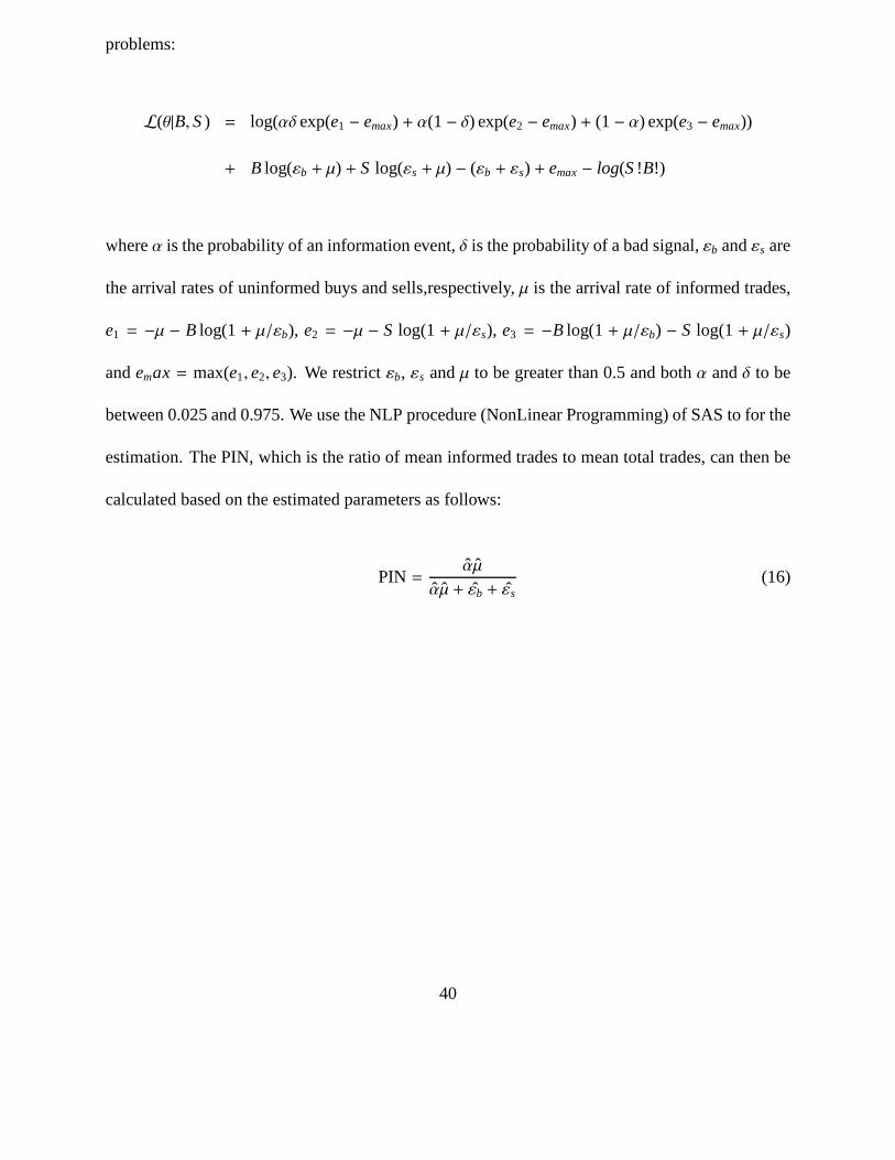
problems:

L(θ|B,S) = log(αδ exp(e1 − emax) + α(1− δ) exp(e2 − emax) + (1− α) exp(e3 − emax))

+ B log(εb + µ) + S log(εs + µ) − (εb + εs) + emax− log(S!B!)

whereα is the probability of an information event,δ is the probability of a bad signal,εb andεs are

the arrival rates of uninformed buys and sells,respectively, µ is the arrival rate of informed trades,

e1 = −µ − B log(1+ µ/εb), e2 = −µ − S log(1+ µ/εs), e3 = −B log(1+ µ/εb) − S log(1+ µ/εs)

andemax = max(e1, e2, e3). We restrictεb, εs andµ to be greater than 0.5 and bothα andδ to be

between 0.025 and 0.975. We use the NLP procedure (NonLinearProgramming) of SAS to for the

estimation. The PIN, which is the ratio of mean informed trades to mean total trades, can then be

calculated based on the estimated parameters as follows:

PIN =α̂µ̂

α̂µ̂ + ε̂b + ε̂s(16)

40

References

Amihud, Y., 2002. Illiquidity and stock returns: Cross-section and time-series effects. Journal of Financial Markets

5 (1), 31–56.

Amihud, Y., Mendelson, H., 1986. Asset pricing and the bid ask spread. Journal of Financial Economics 17 (2),

223–249.

Amihud, Y., Mendelson, H., Pedersen, L. H., 2012. Market liquidity: Asset pricing, risk, and crises. Cambridge

University Press.

Aragon, G. O., Strahan, P. E., 2012. Hedge funds as liquidityproviders: Evidence from the Lehman bankruptcy.

Journal of Financial Economics 103 (3), 570–587.

Beber, A., Pagano, M., 2013. Short-selling bans around the world: Evidence from the 2007-09 crisis. Journal of

Finance 68 (1), 343–381.

Biais, B., Hillion, P., Spatt, C., 1995. An empirical analysis of the limit order book and the order flow in the paris

bourse. Journal of Finance 50 (5), 1655–1689.

Boehmer, E., Jones, C. M., Zhang, X., 2015. Potential pilot problems: Treatment spillovers in financial regulatory

experiments. Unpublished Working Paper., 1–36.

Bollen, N. P., Smith, T., Whaley, R. E., 2004. Modeling the bid/ask spread: Measuring the inventory-holdingpremium.

Journal of Financial Economics 72 (1), 97–141.

Brennan, M., Huh, S.-W., Subrahmanyam, A., 2013. An analysis of the Amihud illiquidity premium. Review of Asset

Pricing Studies 3 (1), 133–176.

Brennan, M. J., Chordia, T., Subrahmanyam, A., Tong, Q., 2012. Sell-order liquidity and the cross-section of expected

stock returns. Journal of Financial Economics 105 (3), 523–541.

Brennan, M. J., Subrahmanyam, A., 1996. Market microstructure and asset pricing: On the compensation for illiquidity

in stock returns. Journal of Financial Economics 41 (3), 441–464.

Brogaard, J., Hendershott, T., Riordan, R., 2014. High-frequency trading and price discovery. Review of Financial

Studies 27 (8), 2267–2306.

Brunnermeier, M. K., Pedersen, L. H., 2009. Market liquidity and funding liquidity. Review of Financial studies 22 (6),

2201–2238.

41

Campbell, J. Y., Hilscher, J., Szilagyi, J., 2008. In searchof distress risk. Journal of Finance 63 (6), 2899–2939.

Cao, C., Hansch, O., Wang, X., 2009. The information contentof an open limit-order book. Journal of Futures Markets

29 (1), 16–41.

Carhart, M. M., 1997. On persistence in mutual fund performance. The Journal of finance 52 (1), 57–82.

Chacko, G. C., Jurek, J. W., Stafford, E., 2008. The price of immediacy. The Journal of Finance63 (3), 1253–1290.

Choi, J. Y., D. Salandro, D., Shastri, K., 1988. On the estimation of bid-ask spreads: Theory and evidence. Journal of

Financial and Quantitative Analysis 23 (2), 219–230.

Chordia, T., Roll, R., Subrahmanyam, A., 2000. Commonalityin liquidity. Journal of Financial Economics 56 (1),

03–28.

Chordia, T., Roll, R., Subrahmanyam, A., 2001. Market liquidity and trading activity. Journal of Finance 56, 501–530.

Chordia, T., Roll, R., Subrahmanyam, A., 2002. Order imbalance, liquidity, and market returns. Journal of Financial

Economics 65 (1), 111–130.

Comerton-Forde, C., Hendershott, T., Jones, C. M., Moulton, P. C., Seasholes, M. S., 2010. Time variation in liquidity:

The role of market-maker inventories and revenues. Journalof Finance 65 (1), 295–331.

Coughenour, J. F., Saad, M. M., 2004. Common market makers and commonality in liquidity. Journal of Financial

Economics 73 (1), 37–69.

Deuskar, P., Johnson, T. C., 2011. Market liquidity and flow-driven risk. Review of Financial Studies 24 (3), 721–753.

Easley, D., Hvidkjaer, S., O’hara, M., 2002. Is informationrisk a determinant of asset returns? The Journal of Finance

57 (5), 2185–2221.

Easley, D., Kiefer, N. M., O’Hara, M., Paperman, J. B., 1996.Liquidity, information, and infrequently traded stocks.

Journal of Finance 51, 1405–1436.

Feldhuetter, P., 2011. The same bond at different prices: Identifying search frictions and selling pressures. Review of

Financial Studies 25 (4), 1155–1206.

Fong, K., Holden, C., Trzcinka, C., 2014. What are the best proxies for global research? Unpublished working paper.

Indiana University.

Garman, M. B., 1976. Market microstructure. Journal of Financial Economics 3 (3), 257–275.

Glosten, L. R., Harris, L. E., 1988. Estimating the components of the bid/ask spread. Journal of Financial Economics

42

21 (1), 123–142.

Glosten, L. R., Milgrom, P. R., 1985. Bid, ask, and transaction prices in a specialist market with heterogeneously

informed agents. Journal of Financial Economics 14 (1), 71–100.

Goettler, R. L., Parlour, C. A., Rajan, U., 2009. Informed traders and limit order markets. Journal of Financial Eco-

nomics 93 (1), 67–87.

Grossman, S. J., Miller, M. H., 1988. Liquidity and market structure. The Journal of Finance 43 (3), 617–633.

Hasbrouck, J., 2004. Liquidity in the futures pits: Inferring market dynamics from incomplete data. Journal of Finan-

cial and Quantitative Analysis 39 (3), 305–326.

Ho, T. S. Y., Macris, R. H., 1984. Dealer bid-ask quotes and transaction prices: An empirical study of some AMEX

options. Journal of Finance 39 (1), 23–45.

Ho, T. S. Y., Stoll, H. R., 1981. Optimal dealer pricing undertransactions and return uncertainty. Journal of Financial

Economics 9 (1), 47–73.

Holden, C., 2009. New low-frequency liquidity measures. Journal of Financial Markets 12 (4), 778–813.

Holden, C. W., Jacobsen, S., 2014. Liquidity measurement problems in fast, competitive markets: Expensive and

cheap solutions. Journal of Finance 69 (4), 1747–1785.

Holden, C. W., Jacobsen, S. E., Subrahmanyam, A., 2014. The empirical analysis of liquidity. Kelley School of

Business Research Paper (2014-09).

Huang, R. D., Stoll, H. R., 1996. Dealer versus auction markets: A paired comparison of execution costs on NASDAQ

and the NYSE. Journal of Financial Economics 41 (3), 313–357.

Irvine, P. J., Benston, G. J., Kandel, E., 2000. Liquidity beyond the inside spread: Measuring and using information in

the limit order book. Available at SSRN 229959.

Jankowitsch, R., Nashikkar, A. J., Subrahmanyam, M. G., 2011. Price dispersion in OTC markets: A new measure of

liquidity. Journal of Banking and Finance 34 (2), 343–357.

Kalay, A., Wohl, A., 2009. Detecting liquidity traders. Journal of Financial and Quantitative Analysis 44 (1), 29–54.

Kamara, A., Lou, X., Sadka, R., 2008. The divergence of liquidity commonality in the cross-section of stocks. Journal

of Financial Economics 89 (3), 444–466.

Karolyi, G. A., Lee, K.-H., Van Dijk, M. A., 2012. Understanding commonality in liquidity around the world. Journal

43

of Financial Economics 105 (1), 82–112.

Korajczyk, R. A., Sadka, R., 2008. Pricing the commonality across alternative measures of liquidity. Journal of Finan-

cial Economics 87 (1), 45–72.

Kyle, A. S., 1985. Continuous auctions and insider trading.Econometrica 53 (6), 1315–1335.

Lee, C., Ready, M., 1991. Inferring trade direction from intraday data. Journal of Finance 46 (2), 733–746.

Lesmond, D. A., Ogden, J. P., Trzcinka, C. A., 1999. A new estimate of transaction costs. Review of Financial Studies

12 (5), 1113–1141.

Lin, H.-W. W., Ke, W.-C., 2011. A computing bias in estimating the probability of informed trading. Journal of

Financial Markets 14, 625–640.

Pastor, L., Stambaugh, R. F., 2003. Liquidity risk and pricediscovery. Journal of Political Economy 111 (3), 642–685.

Petersen, M. A., 2009. Estimating standard errors in financepanel data sets: Comparing approaches. Review of Finan-

cial Studies 22 (1), 435–480.

Roesch, C. G., Kaserer, C., 2014. Reprint of: Market liquidity in the financial crisis: The role of liquidity commonality

and flight-to-quality. Journal of Banking and Finance 45 (1), 152–170.

Roll, R., 1984. A simple implicit measure of the effective bid-ask spread in an efficient market. Journal of Finance

39 (4), 1127–1139.

Rosu, I., 2009. A dynamic model of the limit order book. The Review of Financial Studies 22 (11), 4601–4641.

Stoll, H. R., 1978. The supply of dealer services in securities markets. Journal of Finance 33 (4), 1133–1151.

Whaley, R. E., 2008. Understanding vix. Available at SSRN 1296743.

Wuyts, G., 2008. The impact of liquidity shocks through the limit order book. Unpublished working paper. University

of Leuven.

44

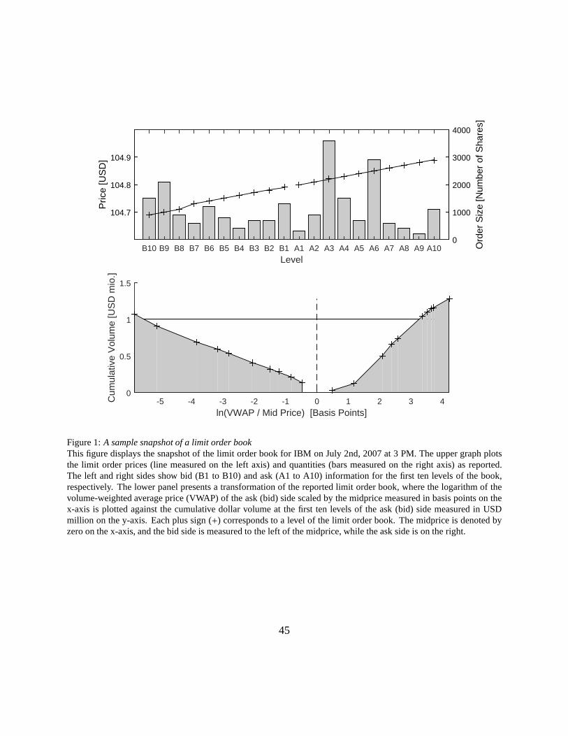
Ord

er S

ize

[Num

ber

of S

hare

s]

0

1000

2000

3000

4000

LevelB10 B9 B8 B7 B6 B5 B4 B3 B2 B1 A1 A2 A3 A4 A5 A6 A7 A8 A9 A10

Pric

e [U

SD

]

104.7

104.8

104.9

ln(VWAP / Mid Price) [Basis Points]-5 -4 -3 -2 -1 0 1 2 3 4C

umul

ativ

e V

olum

e [U

SD

mio

.]

0

0.5

1

1.5

Figure 1:A sample snapshot of a limit order bookThis figure displays the snapshot of the limit order book for IBM on July 2nd, 2007 at 3 PM. The upper graph plotsthe limit order prices (line measured on the left axis) and quantities (bars measured on the right axis) as reported.The left and right sides show bid (B1 to B10) and ask (A1 to A10)information for the first ten levels of the book,respectively. The lower panel presents a transformation ofthe reported limit order book, where the logarithm of thevolume-weighted average price (VWAP) of the ask (bid) side scaled by the midprice measured in basis points on thex-axis is plotted against the cumulative dollar volume at the first ten levels of the ask (bid) side measured in USDmillion on the y-axis. Each plus sign (+) corresponds to a level of the limit order book. The midpriceis denoted byzero on the x-axis, and the bid side is measured to the left of the midprice, while the ask side is on the right.

45

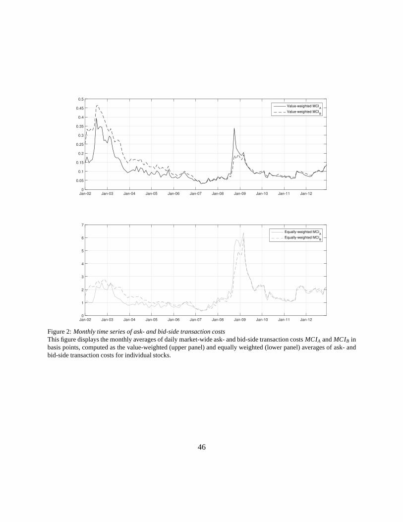
Jan-02 Jan-03 Jan-04 Jan-05 Jan-06 Jan-07 Jan-08 Jan-09 Jan-10 Jan-11 Jan-120

0.05

0.1

0.15

0.2

0.25

0.3

0.35

0.4

0.45

0.5

Value-weighted MCIA

Value-weighted MCIB

Jan-02 Jan-03 Jan-04 Jan-05 Jan-06 Jan-07 Jan-08 Jan-09 Jan-10 Jan-11 Jan-120

1

2

3

4

5

6

7

Equally-weighted MCIA

Equally-weighted MCIB

Figure 2:Monthly time series of ask- and bid-side transaction costsThis figure displays the monthly averages of daily market-wide ask- and bid-side transaction costsMCIA andMCIB inbasis points, computed as the value-weighted (upper panel)and equally weighted (lower panel) averages of ask- andbid-side transaction costs for individual stocks.

46

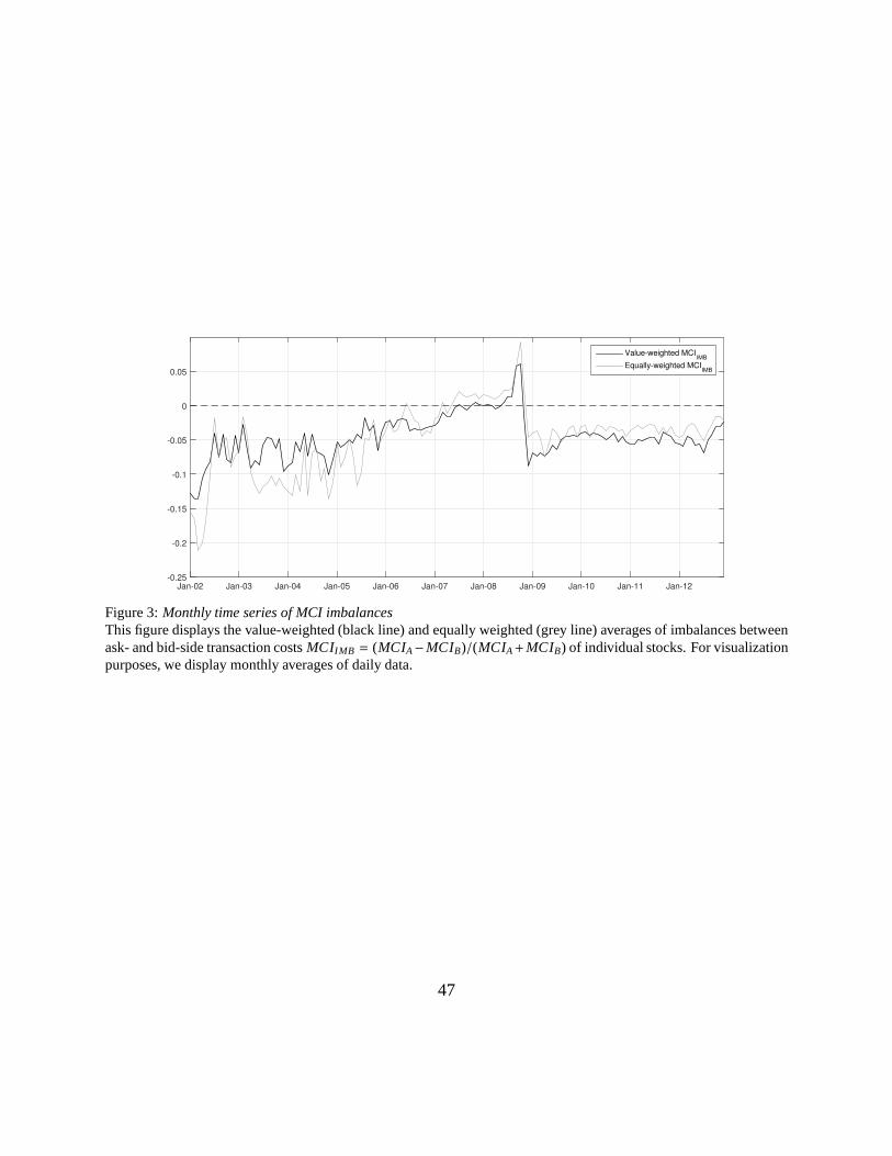
Jan-02 Jan-03 Jan-04 Jan-05 Jan-06 Jan-07 Jan-08 Jan-09 Jan-10 Jan-11 Jan-12-0.25

-0.2

-0.15

-0.1

-0.05

0

0.05

Value-weighted MCIIMB

Equally-weighted MCIIMB

Figure 3:Monthly time series of MCI imbalancesThis figure displays the value-weighted (black line) and equally weighted (grey line) averages of imbalances betweenask- and bid-side transaction costsMCIIMB = (MCIA−MCIB)/(MCIA+MCIB) of individual stocks. For visualizationpurposes, we display monthly averages of daily data.

47

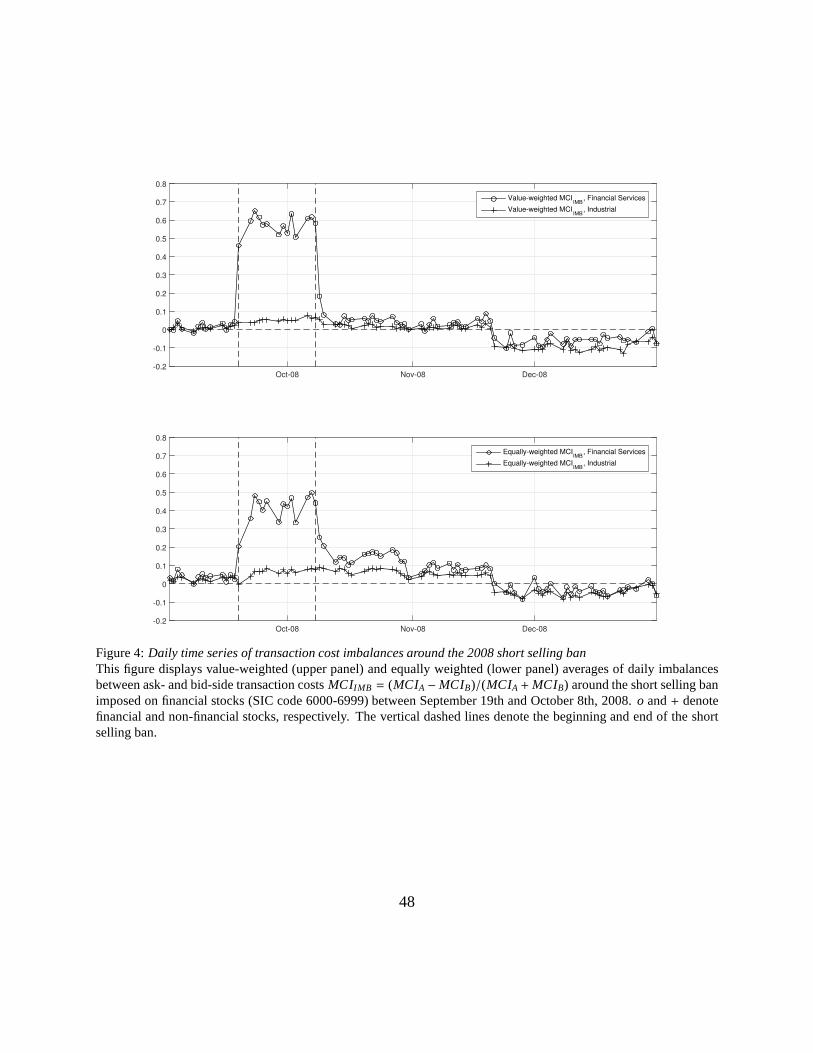
Oct-08 Nov-08 Dec-08-0.2

-0.1

0

0.1

0.2

0.3

0.4

0.5

0.6

0.7

0.8

Value-weighted MCIIMB

, Financial Services

Value-weighted MCIIMB

, Industrial

Oct-08 Nov-08 Dec-08-0.2

-0.1

0

0.1

0.2

0.3

0.4

0.5

0.6

0.7

0.8

Equally-weighted MCIIMB

, Financial Services

Equally-weighted MCIIMB

, Industrial

Figure 4:Daily time series of transaction cost imbalances around the2008 short selling banThis figure displays value-weighted (upper panel) and equally weighted (lower panel) averages of daily imbalancesbetween ask- and bid-side transaction costsMCIIMB = (MCIA −MCIB)/(MCIA+MCIB) around the short selling banimposed on financial stocks (SIC code 6000-6999) between September 19th and October 8th, 2008.o and+ denotefinancial and non-financial stocks, respectively. The vertical dashed lines denote the beginning and end of the shortselling ban.

48

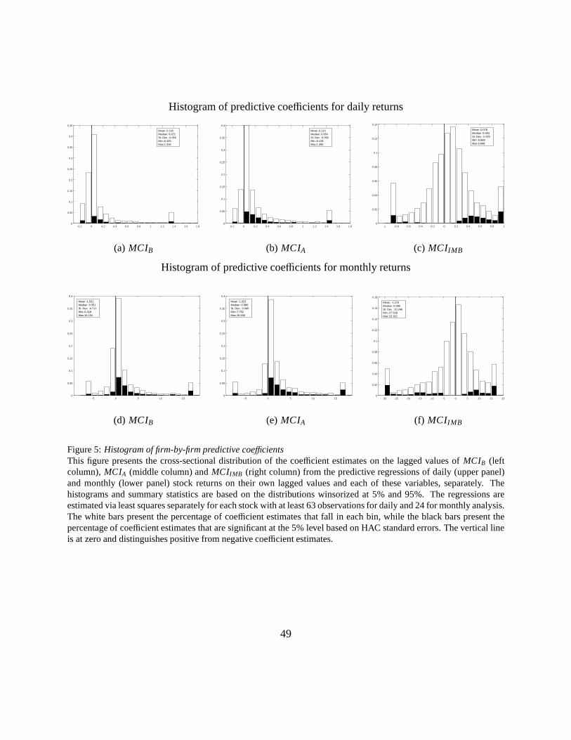
Histogram of predictive coefficients for daily returns

-0.2 0 0.2 0.4 0.6 0.8 1 1.2 1.4 1.6 1.80

0.05

0.1

0.15

0.2

0.25

0.3

0.35

0.4

0.45

Mean :0.140Median :0.022St. Dev. :0.350Min:-0.193Max:1.319

(a) MCIB

-0.2 0 0.2 0.4 0.6 0.8 1 1.2 1.4 1.6 1.80

0.05

0.1

0.15

0.2

0.25

0.3

0.35

0.4

Mean :0.210Median :0.060St. Dev. :0.392Min:-0.139Max:1.494

(b) MCIA

-1 -0.8 -0.6 -0.4 -0.2 0 0.2 0.4 0.6 0.8 10

0.02

0.04

0.06

0.08

0.1

0.12

0.14

Mean :0.078Median :0.094St. Dev. :0.422Min:-0.889Max:0.948

(c) MCIIMB

Histogram of predictive coefficients for monthly returns

-5 0 5 10 150

0.05

0.1

0.15

0.2

0.25

0.3

0.35

0.4

Mean :1.551Median :0.351St. Dev. :4.711Min:-6.318Max:16.154

(d) MCIB

-5 0 5 10 150

0.05

0.1

0.15

0.2

0.25

0.3

0.35

0.4

Mean :1.923Median :0.686St. Dev. :5.045Min:-7.752Max:16.566

(e) MCIA

-30 -25 -20 -15 -10 -5 0 5 10 15 200

0.02

0.04

0.06

0.08

0.1

0.12

0.14

0.16

0.18

Mean :-1.270Median :0.280St. Dev. :10.246Min:-27.509Max:16.182

(f) MCIIMB

Figure 5:Histogram of firm-by-firm predictive coefficientsThis figure presents the cross-sectional distribution of the coefficient estimates on the lagged values ofMCIB (leftcolumn),MCIA (middle column) andMCIIMB (right column) from the predictive regressions of daily (upper panel)and monthly (lower panel) stock returns on their own lagged values and each of these variables, separately. Thehistograms and summary statistics are based on the distributions winsorized at 5% and 95%. The regressions areestimated via least squares separately for each stock with at least 63 observations for daily and 24 for monthly analysis.The white bars present the percentage of coefficient estimates that fall in each bin, while the black bars present thepercentage of coefficient estimates that are significant at the 5% level based on HAC standard errors. The vertical lineis at zero and distinguishes positive from negative coefficient estimates.

49

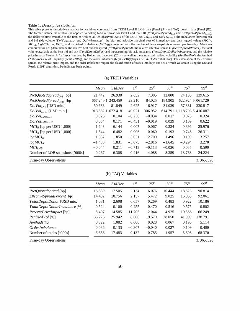
Table 1:Descriptive statistics.This table presents descriptive statistics for variables computed from TRTH Level II LOB data (Panel (A)) and TAQ Level Idata (Panel (B)).The former include the relative (as opposed to dollar) bid-ask spread for level 1 and level 10 (PrctQuotedSpreadL=1 andPrctQuotedSpreadL=10),the dollar volume available at the first, as well as all ten observed levels of the LOB (DolVolL=1 andDolVolL=10), the imbalances between askand bid side volume (DolVolIMB,L=1 and DolVolIMB,L=10), the bid- and ask-side marginal cost of immediacy and theirlogged values (MCIB,MCIA, logMCIA, logMCIB) and its bid-ask imbalance (MCIIMB), together with the number of book snapshots observed per firm-day. Measurescomputed for TAQ data include the relative best bid-ask spread (PrctQuotedSpread), the relative effective spread (EffectiveSpreadPercent), the totalvolume available at the best bid and ask (TotalDepthDollar) and the according bid-ask imbalance (TotalDepthDollarImbalance), and the relativeprice impact (PercentPriceImpact) as used by Holden and Jacobsen (2014), as well as the annualized realized volatility (RealizedVol), the Amihud(2002) measure of illiquidity (AmihudIlliq), and the order imbalance (buys - sells)/(buys+ sells) (OrderImbalance). The calculation of the effectivespread, the relative price impact, and the order imbalance require the classification of trades into buys and sells, which we obtain using the Lee andReady (1991) algorithm.bp indicates basis points.

(a) TRTH Variables

Mean S tdDev 1st 25th 50th 75th 99th

PrctQuotedSpreadL=1 [bp] 21.442 26.938 2.652 7.305 12.808 24.185 139.615PrctQuotedSpreadL=10 [bp] 667.240 1, 243.459 29.210 84.025 184.905 622.924 6, 061.729DolVolL=1 [USD mio.] 50.688 81.849 2.625 16.917 31.039 57.381 330.817DolVolL=10 [USD mio.] 913.882 1, 072.418 49.021 306.952 614.791 1, 118.703 5, 410.087DolVolIMB,L=1 0.025 0.104 −0.236 −0.034 0.017 0.078 0.324DolVolIMB,L=10 0.054 0.171 −0.431 −0.019 0.039 0.109 0.622MCIB [bp per USD 1,000] 1.643 6.144 0.007 0.067 0.224 0.896 25.976MCIA [bp per USD 1,000] 1.544 6.482 0.006 0.060 0.193 0.746 26.311logMCIB −1.352 1.850 −5.031 −2.700 −1.496 −0.109 3.257logMCIA −1.488 1.831 −5.075 −2.816 −1.645 −0.294 3.270MCIIMB −0.044 0.211 −0.713 −0.113 −0.036 0.035 0.590Number of LOB snapshots [’000s] 9.267 6.308 0.216 4.088 8.359 13.763 24.224

Firm-day Observations 3, 365, 528

(b) TAQ Variables

Mean S tdDev 1st 25th 50th 75th 99th

PrctQuotedSpread[bp] 15.839 17.505 2.134 6.076 10.444 18.623 90.814EffectiveSpreadPercent[bp] 14.482 18.756 2.157 5.472 9.025 16.038 92.861TotalDepthDollar[USD mio.] 1.031 2.698 0.057 0.269 0.483 0.922 10.186TotalDepthDollarImbalance[%] 0.524 0.100 0.255 0.470 0.516 0.575 0.802PercentPriceImpact[bp] 8.407 14.585 −11.705 2.044 4.925 10.366 66.249RealizedVol[%] 35.276 25.942 8.606 19.570 28.050 41.909 138.791AmihudIlliq 0.322 1.082 0.006 0.028 0.067 0.190 5.114OrderImbalance 0.036 0.133 −0.307 −0.040 0.027 0.109 0.400Number of trades [’000s] 6.656 17.483 0.132 0.785 1.957 5.698 68.370

Firm-day Observations 3, 365, 528

50

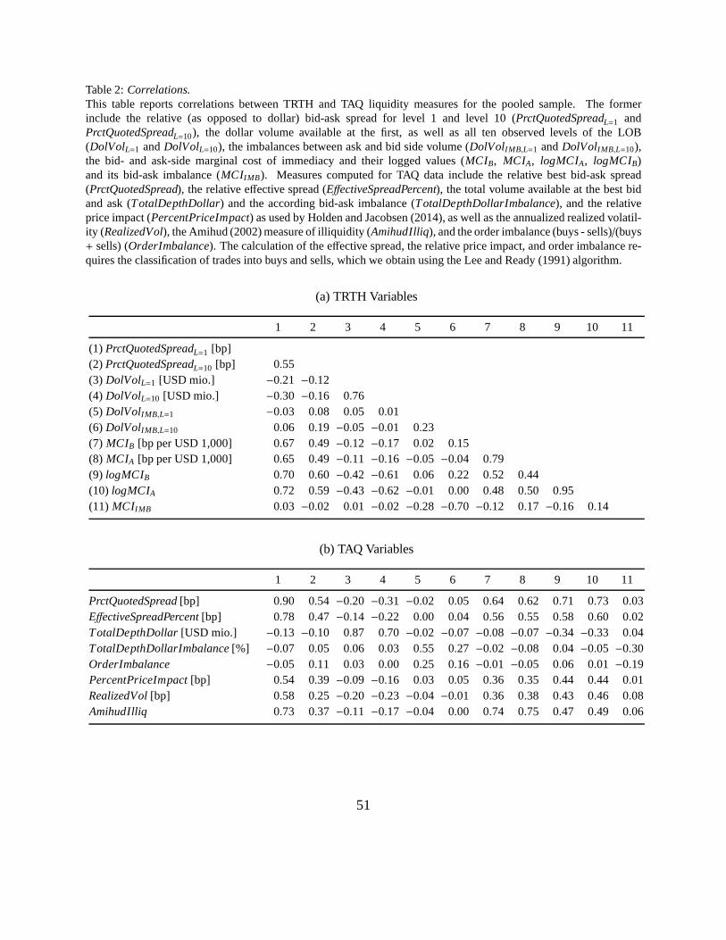
Table 2:Correlations.This table reports correlations between TRTH and TAQ liquidity measures for the pooled sample. The formerinclude the relative (as opposed to dollar) bid-ask spread for level 1 and level 10 (PrctQuotedSpreadL=1 andPrctQuotedSpreadL=10), the dollar volume available at the first, as well as all ten observed levels of the LOB(DolVolL=1 andDolVolL=10), the imbalances between ask and bid side volume (DolVolIMB,L=1 andDolVolIMB,L=10),the bid- and ask-side marginal cost of immediacy and their logged values (MCIB, MCIA, logMCIA, logMCIB)and its bid-ask imbalance (MCIIMB). Measures computed for TAQ data include the relative best bid-ask spread(PrctQuotedSpread), the relative effective spread (EffectiveSpreadPercent), the total volume available at the best bidand ask (TotalDepthDollar) and the according bid-ask imbalance (TotalDepthDollarImbalance), and the relativeprice impact (PercentPriceImpact) as used by Holden and Jacobsen (2014), as well as the annualized realized volatil-ity (RealizedVol), the Amihud (2002) measure of illiquidity (AmihudIlliq), and the order imbalance (buys - sells)/(buys+ sells) (OrderImbalance). The calculation of the effective spread, the relative price impact, and order imbalance re-quires the classification of trades into buys and sells, which we obtain using the Lee and Ready (1991) algorithm.

(a) TRTH Variables

1 2 3 4 5 6 7 8 9 10 11

(1) PrctQuotedSpreadL=1 [bp](2) PrctQuotedSpreadL=10 [bp] 0.55(3) DolVolL=1 [USD mio.] −0.21 −0.12(4) DolVolL=10 [USD mio.] −0.30 −0.16 0.76(5) DolVolIMB,L=1 −0.03 0.08 0.05 0.01(6) DolVolIMB,L=10 0.06 0.19 −0.05 −0.01 0.23(7) MCIB [bp per USD 1,000] 0.67 0.49 −0.12 −0.17 0.02 0.15(8) MCIA [bp per USD 1,000] 0.65 0.49 −0.11 −0.16 −0.05 −0.04 0.79(9) logMCIB 0.70 0.60 −0.42 −0.61 0.06 0.22 0.52 0.44(10) logMCIA 0.72 0.59 −0.43 −0.62 −0.01 0.00 0.48 0.50 0.95(11) MCIIMB 0.03 −0.02 0.01 −0.02 −0.28 −0.70 −0.12 0.17 −0.16 0.14

(b) TAQ Variables

1 2 3 4 5 6 7 8 9 10 11

PrctQuotedSpread[bp] 0.90 0.54 −0.20 −0.31 −0.02 0.05 0.64 0.62 0.71 0.73 0.03EffectiveSpreadPercent[bp] 0.78 0.47 −0.14 −0.22 0.00 0.04 0.56 0.55 0.58 0.60 0.02TotalDepthDollar[USD mio.] −0.13 −0.10 0.87 0.70 −0.02 −0.07 −0.08 −0.07 −0.34 −0.33 0.04TotalDepthDollarImbalance[%] −0.07 0.05 0.06 0.03 0.55 0.27 −0.02 −0.08 0.04 −0.05 −0.30OrderImbalance −0.05 0.11 0.03 0.00 0.25 0.16 −0.01 −0.05 0.06 0.01 −0.19PercentPriceImpact[bp] 0.54 0.39 −0.09 −0.16 0.03 0.05 0.36 0.35 0.44 0.44 0.01RealizedVol[bp] 0.58 0.25 −0.20 −0.23 −0.04 −0.01 0.36 0.38 0.43 0.46 0.08AmihudIlliq 0.73 0.37 −0.11 −0.17 −0.04 0.00 0.74 0.75 0.47 0.49 0.06

51

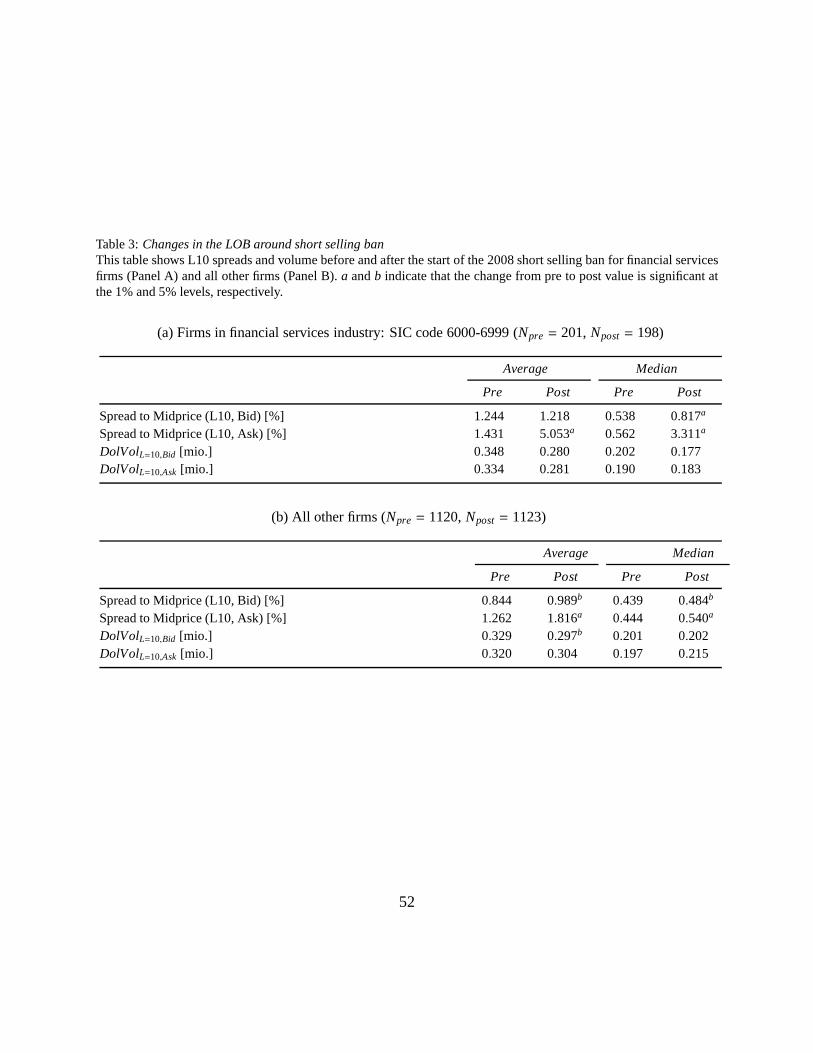
Table 3:Changes in the LOB around short selling banThis table shows L10 spreads and volume before and after the start of the 2008 short selling ban for financial servicesfirms (Panel A) and all other firms (Panel B).a andb indicate that the change from pre to post value is significantatthe 1% and 5% levels, respectively.

(a) Firms in financial services industry: SIC code 6000-6999(Npre = 201,Npost= 198)

Average Median

Pre Post Pre Post

Spread to Midprice (L10, Bid) [%] 1.244 1.218 0.538 0.817a

Spread to Midprice (L10, Ask) [%] 1.431 5.053a 0.562 3.311a

DolVolL=10,Bid [mio.] 0.348 0.280 0.202 0.177DolVolL=10,Ask [mio.] 0.334 0.281 0.190 0.183

(b) All other firms (Npre = 1120,Npost= 1123)

Average Median

Pre Post Pre Post

Spread to Midprice (L10, Bid) [%] 0.844 0.989b 0.439 0.484b

Spread to Midprice (L10, Ask) [%] 1.262 1.816a 0.444 0.540a

DolVolL=10,Bid [mio.] 0.329 0.297b 0.201 0.202DolVolL=10,Ask [mio.] 0.320 0.304 0.197 0.215

52

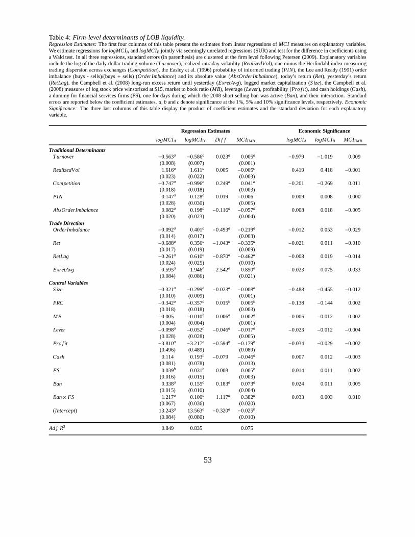
Table 4:Firm-level determinants of LOB liquidity.Regression Estimates:The first four columns of this table present the estimates from linear regressions ofMCI measures on explanatory variables.We estimate regressions forlogMCIA andlogMCIB jointly via seemingly unrelated regressions (SUR) and testfor the difference in coefficients usinga Wald test. In all three regressions, standard errors (in parenthesis) are clustered at the firm level following Petersen (2009). Explanatory variablesinclude the log of the daily dollar trading volume (Turnover), realized intraday volatility (RealizedVol), one minus the Herfindahl index measuringtrading dispersion across exchanges (Competition), the Easley et al. (1996) probability of informed trading (PIN), the Lee and Ready (1991) orderimbalance (buys - sells)/(buys+ sells) (OrderImbalance) and its absolute value (AbsOrderImbalance), today’s return (Ret), yesterday’s return(RetLag), the Campbell et al. (2008) long-run excess return until yesterday (ExretAvg), logged market capitalization (S ize), the Campbell et al.(2008) measures of log stock price winsorized at $15, marketto book ratio (MB), leverage (Lever), profitability (Pro f it), and cash holdings (Cash),a dummy for financial services firms (FS), one for days during which the 2008 short selling ban was active (Ban), and their interaction. Standarderrors are reported below the coefficient estimates.a, b andc denote significance at the 1%, 5% and 10% significance levels,respectively.EconomicSignificance: The three last columns of this table display the product of coefficient estimates and the standard deviation for each explanatoryvariable.

Regression Estimates Economic Significance

logMCIA logMCIB Di f f MCI IMB logMCIA logMCIB MCIIMB

Traditional DeterminantsTurnover −0.563a −0.586a 0.023a 0.005a −0.979 −1.019 0.009

(0.008) (0.007) (0.001)RealizedVol 1.616a 1.611a 0.005 −0.005c 0.419 0.418 −0.001

(0.023) (0.022) (0.003)Competition −0.747a −0.996a 0.249a 0.041a −0.201 −0.269 0.011

(0.018) (0.018) (0.003)PIN 0.147a 0.128a 0.019 −0.006 0.009 0.008 0.000

(0.028) (0.030) (0.005)AbsOrderImbalance 0.082a 0.198a −0.116a −0.057a 0.008 0.018 −0.005

(0.020) (0.023) (0.004)Trade Direction

OrderImbalance −0.092a 0.401a −0.493a −0.219a −0.012 0.053 −0.029(0.014) (0.017) (0.003)

Ret −0.688a 0.356a −1.043a −0.335a −0.021 0.011 −0.010(0.017) (0.019) (0.009)

RetLag −0.261a 0.610a −0.870a −0.462a −0.008 0.019 −0.014(0.024) (0.025) (0.010)

ExretAvg −0.595a 1.946a −2.542a −0.850a −0.023 0.075 −0.033(0.084) (0.086) (0.021)

Control VariablesS ize −0.321a −0.299a −0.023a −0.008a −0.488 −0.455 −0.012

(0.010) (0.009) (0.001)PRC −0.342a −0.357a 0.015b 0.005b −0.138 −0.144 0.002

(0.018) (0.018) (0.003)MB −0.005 −0.010b 0.006a 0.002a −0.006 −0.012 0.002

(0.004) (0.004) (0.001)Lever −0.098a −0.052c −0.046a −0.017a −0.023 −0.012 −0.004

(0.028) (0.028) (0.005)Pro f it −3.810a −3.217a −0.594b −0.179b −0.034 −0.029 −0.002

(0.496) (0.489) (0.089)Cash 0.114 0.193b −0.079 −0.046a 0.007 0.012 −0.003

(0.081) (0.078) (0.013)FS 0.039b 0.031b 0.008 0.005b 0.014 0.011 0.002

(0.016) (0.015) (0.003)Ban 0.338a 0.155a 0.183a 0.073a 0.024 0.011 0.005

(0.015) (0.010) (0.004)Ban× FS 1.217a 0.100a 1.117a 0.382a 0.033 0.003 0.010

(0.067) (0.036) (0.020)(Intercept) 13.243a 13.563a −0.320a −0.025b

(0.084) (0.080) (0.010)

Ad j. R2 0.849 0.835 0.075

53

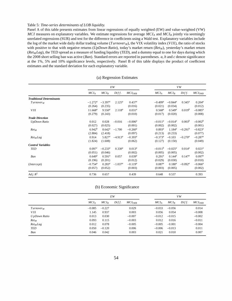
Table 5:Time-series determinants of LOB liquidity.Panel A of this table presents estimates from linear regressions of equally weighted (EW) and value-weighted (VW)MCI measures on explanatory variables. We estimate regressions for averageMCIA andMCIB jointly via seeminglyunrelated regressions (SUR) and test for the difference in coefficients using a Wald test. Explanatory variables includethe log of the market wide daily dollar trading volume (TurnoverM), the VIX volatility index (VIX), the ratio of stockswith positive to that with negative returns (UpDown Ratio), today’s market return (RetM), yesterday’s market return(RetMLag), the TED spread as a measure of funding liquidity (TED), and a dummy equal to one for days during whichthe 2008 short selling ban was active (Ban). Standard errors are reported in parentheses.a, b andc denote significanceat the 1%, 5% and 10% significance levels, respectively. Panel B of this table displays the product of coefficientestimates and the standard deviation for each explanatory variable.

(a) Regression Estimates

EW VW

MCIA MCIB Di f f . MCIIMB MCIA MCIB Di f f . MCIIMB

Traditional DeterminantsTurnoverM −1.272a −3.397a 2.125a 0.437a −0.499a −0.844a 0.345a 0.204a

(0.264) (0.235) (0.016) (0.021) (0.034) (0.012)VIX 11.668a 9.550a 2.118a 0.031a 0.568a 0.549a 0.019b −0.085a

(0.279) (0.243) (0.010) (0.017) (0.020) (0.008)Trade Direction

UpDown Ratio 0.012 0.028 −0.016 −0.006a −0.011a −0.014a 0.003b −0.002b

(0.027) (0.025) (0.001) (0.002) (0.002) (0.001)RetM 6.942b 8.642a −1.700 −0.260a 0.893a 1.184a −0.291b −0.823a

(2.884) (2.418) (0.097) (0.213) (0.233) (0.077)RetM Lag 0.914 5.827a −4.913a −0.393a −0.373a −0.103 −0.270a −0.287a

(1.824) (1.608) (0.062) (0.127) (0.150) (0.049)Control Variables

TED 0.097c −0.233a 0.330a 0.013a −0.011b −0.025a 0.014a 0.021a

(0.051) (0.046) (0.002) (0.005) (0.005) (0.002)Ban 0.649a 0.591a 0.057 0.039a 0.291a 0.144a 0.147a 0.097a

(0.196) (0.201) (0.012) (0.029) (0.030) (0.010)(Intercept) −0.754a 0.283a −1.037a −0.119a 0.087a 0.180a −0.092a −0.066a

(0.057) (0.052) (0.003) (0.003) (0.005) (0.002)

Ad j. R2 0.736 0.657 0.439 0.648 0.537 0.393

(b) Economic Significance

EW VW

MCIA MCIB Di f f . MCIIMB MCIA MCIB Di f f . MCIIMB

TurnoverM −0.085 −0.227 0.029 −0.033 −0.056 0.014VIX 1.145 0.937 0.003 0.056 0.054 −0.008U pDown Ratio 0.013 0.030 −0.007 −0.012 −0.015 −0.002RetM 0.093 0.115 −0.003 0.012 0.016 −0.011RetM Lag 0.012 0.078 −0.005 −0.005 −0.001 −0.004TED 0.050 −0.120 0.006 −0.006 −0.013 0.011Ban 0.046 0.042 0.003 0.021 0.010 0.007

54

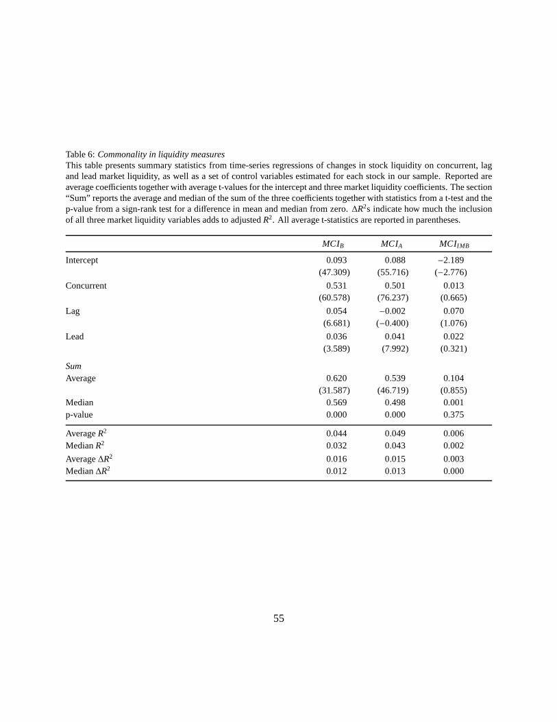
Table 6:Commonality in liquidity measuresThis table presents summary statistics from time-series regressions of changes in stock liquidity on concurrent, lagand lead market liquidity, as well as a set of control variables estimated for each stock in our sample. Reported areaverage coefficients together with average t-values for the intercept andthree market liquidity coefficients. The section“Sum” reports the average and median of the sum of the three coefficients together with statistics from a t-test and thep-value from a sign-rank test for a difference in mean and median from zero.∆R2s indicate how much the inclusionof all three market liquidity variables adds to adjustedR2. All average t-statistics are reported in parentheses.

MCIB MCIA MCIIMB

Intercept 0.093 0.088 −2.189(47.309) (55.716) (−2.776)

Concurrent 0.531 0.501 0.013(60.578) (76.237) (0.665)

Lag 0.054 −0.002 0.070(6.681) (−0.400) (1.076)

Lead 0.036 0.041 0.022(3.589) (7.992) (0.321)

SumAverage 0.620 0.539 0.104

(31.587) (46.719) (0.855)Median 0.569 0.498 0.001p-value 0.000 0.000 0.375

AverageR2 0.044 0.049 0.006MedianR2 0.032 0.043 0.002

Average∆R2 0.016 0.015 0.003Median∆R2 0.012 0.013 0.000

55

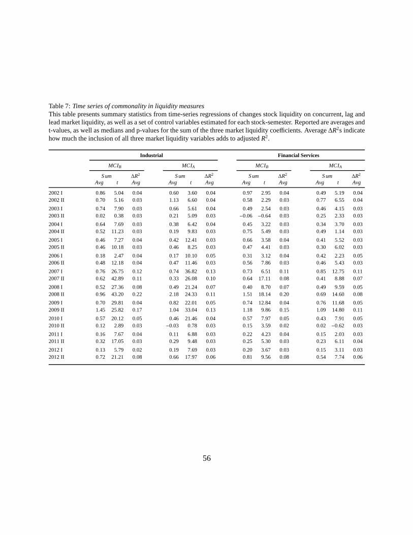
Table 7:Time series of commonality in liquidity measuresThis table presents summary statistics from time-series regressions of changes stock liquidity on concurrent, lag andlead market liquidity, as well as a set of control variables estimated for each stock-semester. Reported are averages andt-values, as well as medians and p-values for the sum of the three market liquidity coefficients. Average∆R2s indicatehow much the inclusion of all three market liquidity variables adds to adjustedR2.

Industrial Financial Services

MCIB MCIA MCIB MCIA

S um ∆R2 S um ∆R2 S um ∆R2 S um ∆R2

Avg t Avg Avg t Avg Avg t Avg Avg t Avg

2002 I 0.86 5.04 0.04 0.60 3.60 0.04 0.97 2.95 0.04 0.49 5.19 0.042002 II 0.70 5.16 0.03 1.13 6.60 0.04 0.58 2.29 0.03 0.77 6.55 0.04

2003 I 0.74 7.90 0.03 0.66 5.61 0.04 0.49 2.54 0.03 0.46 4.15 0.032003 II 0.02 0.38 0.03 0.21 5.09 0.03 −0.06 −0.64 0.03 0.25 2.33 0.03

2004 I 0.64 7.69 0.03 0.38 6.42 0.04 0.45 3.22 0.03 0.34 3.70 0.032004 II 0.52 11.23 0.03 0.19 9.83 0.03 0.75 5.49 0.03 0.49 1.14 0.03

2005 I 0.46 7.27 0.04 0.42 12.41 0.03 0.66 3.58 0.04 0.41 5.52 0.032005 II 0.46 10.18 0.03 0.46 8.25 0.03 0.47 4.41 0.03 0.30 6.02 0.03

2006 I 0.18 2.47 0.04 0.17 10.10 0.05 0.31 3.12 0.04 0.42 2.23 0.052006 II 0.48 12.18 0.04 0.47 11.46 0.03 0.56 7.86 0.03 0.46 5.43 0.03

2007 I 0.76 26.75 0.12 0.74 36.82 0.13 0.73 6.51 0.11 0.85 12.75 0.112007 II 0.62 42.89 0.11 0.33 26.08 0.10 0.64 17.11 0.08 0.41 8.88 0.07

2008 I 0.52 27.36 0.08 0.49 21.24 0.07 0.40 8.70 0.07 0.49 9.59 0.052008 II 0.96 43.20 0.22 2.18 24.33 0.11 1.51 18.14 0.20 0.69 14.60 0.08

2009 I 0.70 29.81 0.04 0.82 22.01 0.05 0.74 12.84 0.04 0.76 11.68 0.052009 II 1.45 25.82 0.17 1.04 33.04 0.13 1.18 9.86 0.15 1.09 14.80 0.11

2010 I 0.57 20.12 0.05 0.46 21.46 0.04 0.57 7.97 0.05 0.43 7.91 0.052010 II 0.12 2.89 0.03 −0.03 0.78 0.03 0.15 3.59 0.02 0.02 −0.62 0.03

2011 I 0.16 7.67 0.04 0.11 6.88 0.03 0.22 4.23 0.04 0.15 2.03 0.032011 II 0.32 17.05 0.03 0.29 9.48 0.03 0.25 5.30 0.03 0.23 6.11 0.04

2012 I 0.13 5.79 0.02 0.19 7.69 0.03 0.20 3.67 0.03 0.15 3.11 0.032012 II 0.72 21.21 0.08 0.66 17.97 0.06 0.81 9.56 0.08 0.54 7.74 0.06

56

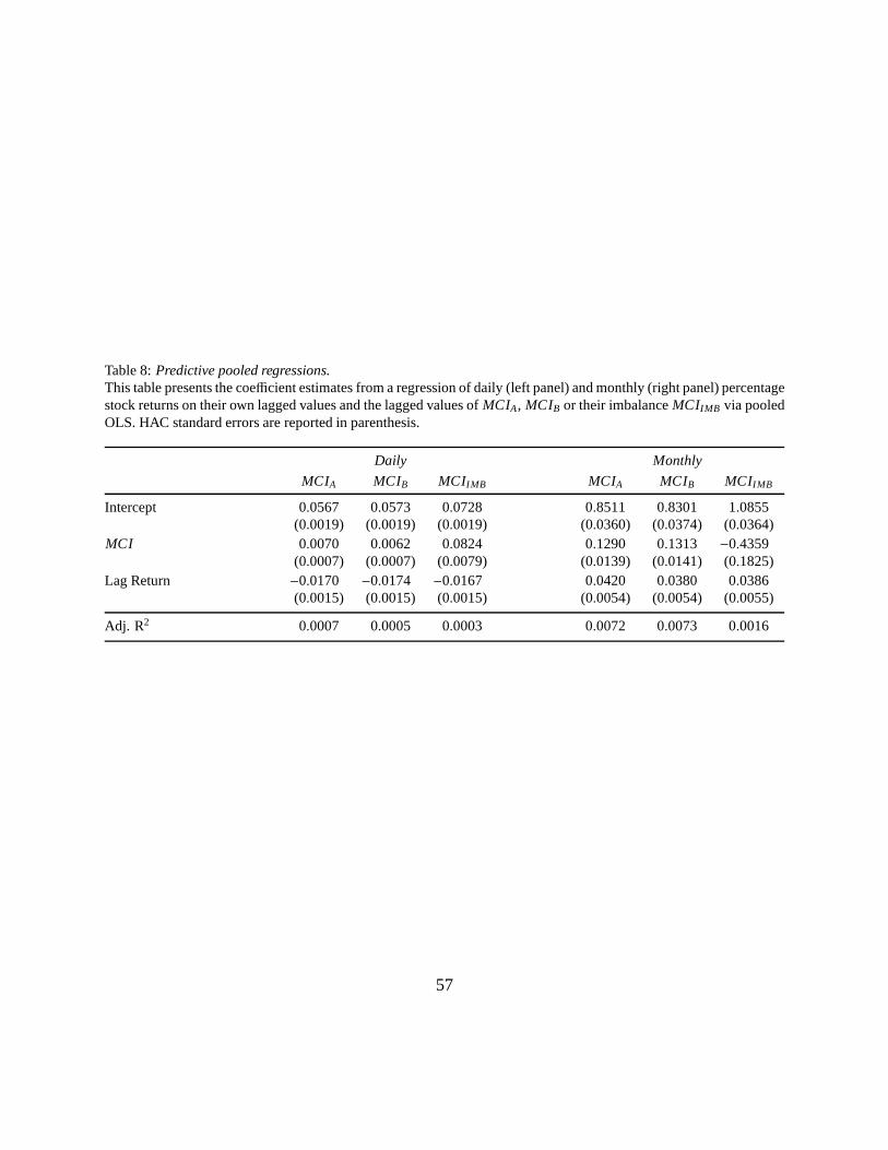
Table 8:Predictive pooled regressions.This table presents the coefficient estimates from a regression of daily (left panel) and monthly (right panel) percentagestock returns on their own lagged values and the lagged values of MCIA, MCIB or their imbalanceMCIIMB via pooledOLS. HAC standard errors are reported in parenthesis.

Daily Monthly

MCIA MCIB MCIIMB MCIA MCIB MCIIMB

Intercept 0.0567 0.0573 0.0728 0.8511 0.8301 1.0855(0.0019) (0.0019) (0.0019) (0.0360) (0.0374) (0.0364)

MCI 0.0070 0.0062 0.0824 0.1290 0.1313 −0.4359(0.0007) (0.0007) (0.0079) (0.0139) (0.0141) (0.1825)

Lag Return −0.0170 −0.0174 −0.0167 0.0420 0.0380 0.0386(0.0015) (0.0015) (0.0015) (0.0054) (0.0054) (0.0055)

Adj. R2 0.0007 0.0005 0.0003 0.0072 0.0073 0.0016

57

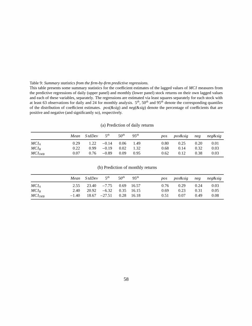
Table 9:Summary statistics from the firm-by-firm predictive regressions.This table presents some summary statistics for the coefficient estimates of the lagged values ofMCI measures fromthe predictive regressions of daily (upper panel) and monthly (lower panel) stock returns on their own lagged valuesand each of these variables, separately. The regressions are estimated via least squares separately for each stock withat least 63 observations for daily and 24 for monthly analysis. 5th, 50th and 95th denote the corresponding quantilesof the distribution of coefficient estimates.pos(& sig) andneg(& sig) denote the percentage of coefficients that arepositive and negative (and significantly so), respectively.

(a) Prediction of daily returns

Mean S tdDev 5th 50th 95th pos pos& sig neg neg& sig

MCIA 0.29 1.22 −0.14 0.06 1.49 0.80 0.25 0.20 0.01MCIB 0.22 0.99 −0.19 0.02 1.32 0.68 0.14 0.32 0.03MCIIMB 0.07 0.76 −0.89 0.09 0.95 0.62 0.12 0.38 0.03

(b) Prediction of monthly returns

Mean S tdDev 5th 50th 95th pos pos& sig neg neg& sig

MCIA 2.55 23.40 −7.75 0.69 16.57 0.76 0.29 0.24 0.03MCIB 2.40 20.92 −6.32 0.35 16.15 0.69 0.23 0.31 0.05MCIIMB −1.40 18.67 −27.51 0.28 16.18 0.51 0.07 0.49 0.08

58

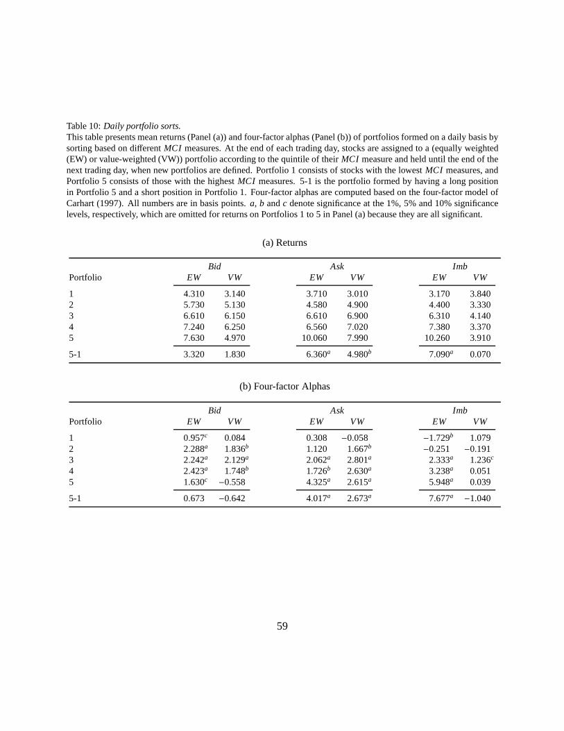
Table 10:Daily portfolio sorts.This table presents mean returns (Panel (a)) and four-factor alphas (Panel (b)) of portfolios formed on a daily basis bysorting based on differentMCI measures. At the end of each trading day, stocks are assignedto a (equally weighted(EW) or value-weighted (VW)) portfolio according to the quintile of theirMCI measure and held until the end of thenext trading day, when new portfolios are defined. Portfolio1 consists of stocks with the lowestMCI measures, andPortfolio 5 consists of those with the highestMCI measures. 5-1 is the portfolio formed by having a long positionin Portfolio 5 and a short position in Portfolio 1. Four-factor alphas are computed based on the four-factor model ofCarhart (1997). All numbers are in basis points.a, b andc denote significance at the 1%, 5% and 10% significancelevels, respectively, which are omitted for returns on Portfolios 1 to 5 in Panel (a) because they are all significant.

(a) Returns

Bid Ask ImbPortfolio EW VW EW VW EW VW

1 4.310 3.140 3.710 3.010 3.170 3.8402 5.730 5.130 4.580 4.900 4.400 3.3303 6.610 6.150 6.610 6.900 6.310 4.1404 7.240 6.250 6.560 7.020 7.380 3.3705 7.630 4.970 10.060 7.990 10.260 3.910

5-1 3.320 1.830 6.360a 4.980b 7.090a 0.070

(b) Four-factor Alphas

Bid Ask ImbPortfolio EW VW EW VW EW VW

1 0.957c 0.084 0.308 −0.058 −1.729b 1.0792 2.288a 1.836b 1.120 1.667b −0.251 −0.1913 2.242a 2.129a 2.062a 2.801a 2.333a 1.236c

4 2.423a 1.748b 1.726b 2.630a 3.238a 0.0515 1.630c −0.558 4.325a 2.615a 5.948a 0.039

5-1 0.673 −0.642 4.017a 2.673a 7.677a −1.040

59

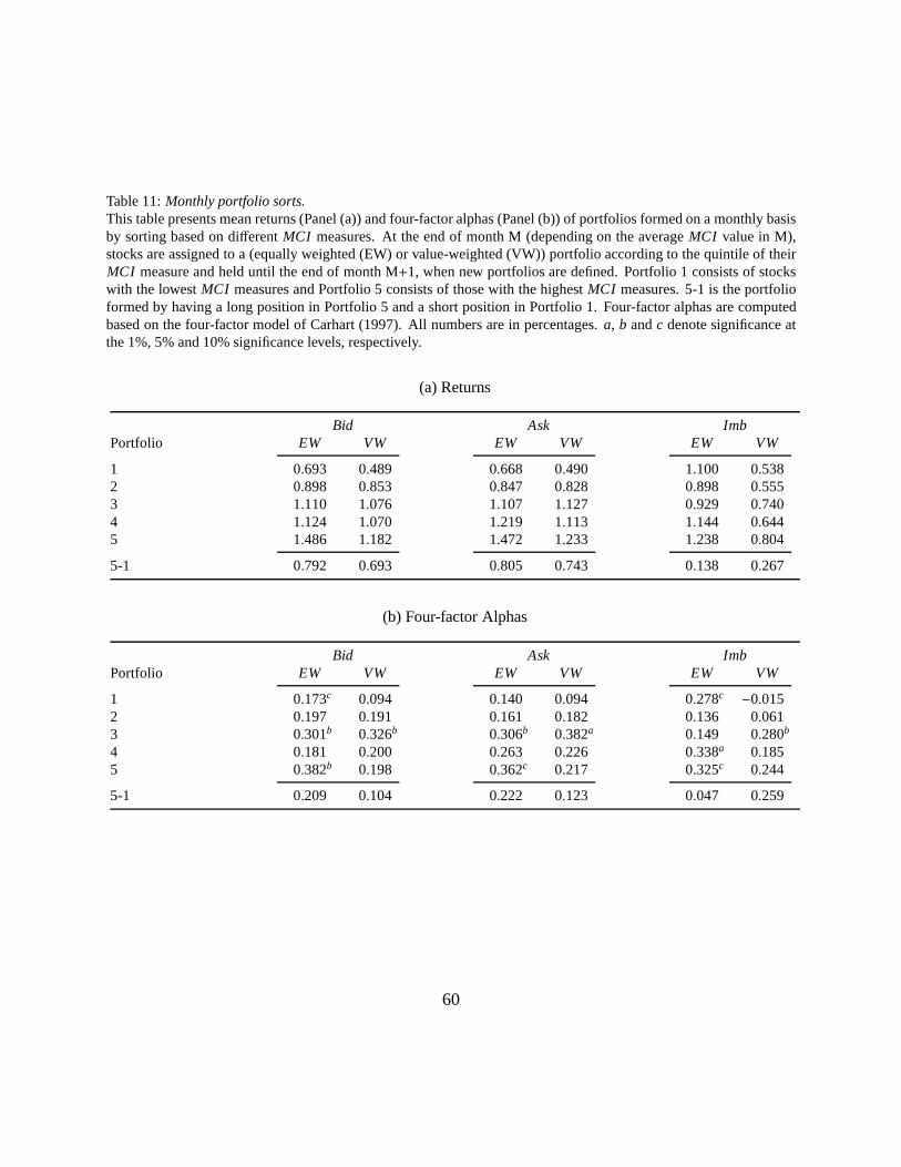
Table 11:Monthly portfolio sorts.This table presents mean returns (Panel (a)) and four-factor alphas (Panel (b)) of portfolios formed on a monthly basisby sorting based on differentMCI measures. At the end of month M (depending on the averageMCI value in M),stocks are assigned to a (equally weighted (EW) or value-weighted (VW)) portfolio according to the quintile of theirMCI measure and held until the end of month M+1, when new portfolios are defined. Portfolio 1 consists of stockswith the lowestMCI measures and Portfolio 5 consists of those with the highestMCI measures. 5-1 is the portfolioformed by having a long position in Portfolio 5 and a short position in Portfolio 1. Four-factor alphas are computedbased on the four-factor model of Carhart (1997). All numbers are in percentages.a, b andc denote significance atthe 1%, 5% and 10% significance levels, respectively.

(a) Returns

Bid Ask ImbPortfolio EW VW EW VW EW VW

1 0.693 0.489 0.668 0.490 1.100 0.5382 0.898 0.853 0.847 0.828 0.898 0.5553 1.110 1.076 1.107 1.127 0.929 0.7404 1.124 1.070 1.219 1.113 1.144 0.6445 1.486 1.182 1.472 1.233 1.238 0.804

5-1 0.792 0.693 0.805 0.743 0.138 0.267

(b) Four-factor Alphas

Bid Ask ImbPortfolio EW VW EW VW EW VW

1 0.173c 0.094 0.140 0.094 0.278c −0.0152 0.197 0.191 0.161 0.182 0.136 0.0613 0.301b 0.326b 0.306b 0.382a 0.149 0.280b

4 0.181 0.200 0.263 0.226 0.338a 0.1855 0.382b 0.198 0.362c 0.217 0.325c 0.244

5-1 0.209 0.104 0.222 0.123 0.047 0.259

60