Embed Size (px)
Citation preview

BICYCLE LEVEL OF SERVICE IN URBAN
INDIAN CONTEXT
MINAKSHI SHESHADRI NAYAK
DEPARTMENT OF CIVIL ENGINEERING
NATIONAL INSTITUTE OF TECHNOLOGY
ROURKELA-769008, ODISHA
MAY 2013
BICYCLE LEVEL OF SERVICE IN URBAN INDIAN CONTEXT
Thesis
Submitted in partial fulfillment of the requirements
For the degree of
Master of Technology
in
Transportation Engineering
By
Minakshi Sheshadri Nayak
Roll no-211CE3245
Under guidance of
Prof. P.K Bhuyan
DEPARMENT OF CIVIL ENGINEERING
NATIONAL INSTITUTE OF TECHNOLOGY
ROURKELA-769008
2013

i
NATIONAL INSTITUTE OFTECHNOLOGY ROURKELA – 769008
CERTIFICATE
This is to certify that project entitled “Bicycle Level of Service in Urban Indian Context” submitted by MINAKSHI SHESHADRI NAYAK in partial fulfillment of the requirements for the award of Master Of Technology Degree in Civil Engineering with specialization in Transportation Engineering at National Institute of Technology, Rourkela is an authentic work carried out by her under my personal supervision and guidance. To the best of my knowledge the matter embodied in this project review report has not been submitted in any other university /institute for award of any Degree or Diploma.
Prof. P.K Bhuyan
Department of civil engineering
National Institute of Technology,
Rourkela -769008

ii
ACKNOWLEDGEMENT
First and foremost, I am deeply indebted to Dr. P.K Bhuyan my advisor and guide, for the
motivation, guidance, tutelage and patience throughout the research work. I appreciate his broad
range of expertise and attention to detail, as well as the constant encouragement he has given me
over the years. There is no need to mention that a big part of this thesis is the result of joint work
with him, without which the completion of the work would have been impossible.
My sincere thanks to Prof. M. Panda former HOD of Civil Engineering Department, NIT
Rourkela and Dr. U. Chattaraj for providing valuable co-operation and needed advice
generously all along my M.Tech study.
I would like to extend my gratefulness to Dr. S. Sarangi, Director, NIT Rourkela and Dr. N.
Roy, HOD, Civil Engineering Department, NIT Rourkela for providing the necessary facilities
for my research work.
I also want to convey sincere thanks to all my friends of the Transportation Engineering
Specialization for their co-operation and cheering up ability which made this project work
smooth. I apologize, if I have forgotten anyone.
Last but not the least, my parents and the one above all of us, the omnipresent God, for the
blessing that has been bestowed upon me in all my endeavours.
Minakshi Sheshadri Nayak
Roll No-211CE3245

iii
Abstract
India is a developing country the traffic especially in urban streets is very much heterogeneous
consisting various kinds of vehicles having different operational characteristics. Bicycle level of
service (BLOS) identifies the quality of service for bicyclists that currently exists within the
roadway environment. Because of poor traffic management and un-planned lane space utilization
BLOS is decreased. For the safe and convenient traffic flow, it is necessary to measure the Level
of Service (LOS) of the bicyclist for urban roads in Indian context. At present BLOS ranges for
LOS categories are not well defined for highly heterogeneous traffic flow on urban streets in
Indian context. In this study, accordingly, an attempt has been made to arrive at suitable criteria
for the BLOS analysis of urban on-streets. In the present study the basic premise of urban streets
and BLOS are discussed. Literatures from various sources are collected and an in-depth review
on analysis of BLOS is carried out.The video camera was employed to collect the data sets of 35
segments from two cities, Rourkela and Bhubaneswar of Odisha State, India. The average
effective width of the outside through lane, motorized vehicle volumes, motorized vehicle
speeds, heavy vehicle (truck) volumes, pavement conditionand percentage of on street parking
are considered as the influencing factors in defining levels of service criteria of bicyclist in urban
street. Emphasis is put on the calibration of BLOS model developed by the Florida Department
of Transportation in classifying the levels of service of the bicyclist provided by road
infrastructure. The collected data are used to calibrate the BLOS model to find the BLOS score
of each road segment. Calibrated model coefficients appropriate in Indian context are determined
using multivariate regression analysis. In order to define levels of service provided by urban on-
street segments, BLOS scores are classified into six categories (A-F) using k-mean, HAC, fuzzy
c-means,Affinity Propagation (AP), Self Organizing Map (SOM) and GA-fuzzy clustering

iv
methods. These clustering methods show different BLOS ranges for service categories.
However, to know the most appropriate clustering technique applicable in Indian context,
Average Silhouette Width (ASW) is calculated for every clustering method. After a thorough
investigation it is induced that K-meanclustering method is the most appropriate one to define
BLOS categories. The defined BLOS score ranges in this study are observed to be higher than
that witnessed by FDOT studies; implies the kind of service the bicyclist perceived in urban
Indian context is inferior to that observed by FDOT. From all the factors that affect BLOS score,
“effective width of outside through lane” affect the most. The study concludes that bicyclist
travel, more often, at the poor quality of service of “D”, “E” and “F”, than good quality of
service of “A”, “B” and “C”. This may be due to lack of proper attention by the planners and
developers towards bicycle facilities in urban Indian context.
Keywords: Urban Street segment, BLOS, BLOS score, K-means clustering, Hierarchical
agglomerative clustering, Fuzzy c-means clustering, Affinity Propagation clustering, Self
Organizing Map clustering, GA-fuzzy clustering and Average Silhouette Width.
v
Contents
Items Page No.
Certificate i
Acknowledgement ii
Abstract iii
Contents v
List of Figures ix
List of Tables xi
Abbreviations xii
1. Introduction 1-6
1.1 General 1
1.2 Statement of the Problem 5
1.3 Objectives 5
1.4 Organization of the Report 6
2. Urban Streets and Bicycle Level of Service Concepts 7-11
3. Review of Literature 12-22
3.1 General 12

vi
3.2 Bicyclist Safety and LOS 12
3.3 Intersection Bicycle LOS 14
3.4 Shared On-Street LOS 15
3.5 Quality of Service using Perception of Bicyclist 17
3.6 Modeling and Simulation 19
4. Cluster Analysis 23-42
4.1 Introduction 23
4.2 Cluster Partitions 23
4.2.1 Hard partition 24
4.2.2 Fuzzy partition 25
4.3 Methods of Cluster Analysis 25
4.3.1 K-means clustering 26
4.3.2 Fuzzy c-means clustering 28
4.3.3 Hierarchical agglomerative clustering 33
4.3.4 Affinity Propagation (AP) clustering 36
4.3.5 GA-Fuzzy Algorithm 37
4.3.6 Self-organizing map (SOM) clustering 40
4.4 Cluster Validation Measure: Silhouettes 41
4.5 Average silhouette width 41

vii
5. Methodology 43-49
5.1 Bicycle Level of Service (BLOS) Model 43
5.2 Terms used in BLOS model 47
6. Study Area and Data Collection 50-54
6.1 Introduction 50
6.2 study corridor and data collection 50
6.2.1 Study corridor 50
6.2.2 Data collection 53
7. Results of Cluster Analysis for LOS Criteria 55-68
7.1 Introduction 55
7.1.1 K-means Clustering 55
7.1.2 Hierarchical Agglomerative Clustering (HAC) 57
7.1.3 Fuzzy C-Means (FCM) Clustering 59
7.1.4Affinity Propagation (AP) clustering 62
7.1.5 GA-Fuzzy Algorithm 63
7.1.6 Self-organizing map (SOM) clustering 64

viii
8. Summary, Conclusions and Future Scope 69-71
8.1 Summary 69
8.2 Conclusion 70
8.3 Contributions 71
8.4 Applications 71
8.5 Limitations and Future Scope 71
References 73-80
List of Publications 81

ix
List of Figures
Figure No. Page No.
1.1 Overall framework of the study 4
2.1 Representing various types of bicycle lane 10
2.2 The designated bicycle lane with pavement marking 11
2.3 Cycle prohibited by IRC-67 11
4.1 Flowchart of AP Clustering 36
5.1 Co-relationship between influencing attributes and BLOS 44
5.2 Width of pavement for the outside lane and shoulder (Wt) 48
(Two lane undivided)
5.3 Width of pavement for the outside lane and shoulder (Wt) 48
(For multilane road)
6.1 Map showing the road segments of data collection for 51
Rourkela city
6.2 Map showing the road segments of data collection for 51
for Bhubaneswar city
6.3 D –block(Koel Nager) to Police station ,Rorkela Jiripani 52
6.4 Jan path road, Bhubaneswar 52
6.5 Ring Road, Rourkela 52
6.6 AG chowk to PMG chowk, Bhubaneswar Bhubaneswar 52
6.7 Handycam fitted on a tripod stand 53

x
7.1 K-Means clustering of BLOS Scores 56
7.2 Silhouettes Plot of BLOS Scores using K-Means Clustering 56
7.3 HAC of BLOS Scores 58
7.4 Silhouettes Plot of BLOS Scores using HAC 58
7.5 Dendogram using HAC on bicycle score data 59
7.6 FCM Clustering of BLOS Scores 61
7.7 Silhouettes Plot of BLOS Scores using FCM Clustering 61
7.8 Plot for bicycle LOS for Urban Street segments using Affinity 63
Propagation (AP) clustering
7.9 Plot for bicycle LOS for Urban Street segments using 64
GA-Fuzzy clustering
7.10 Plot for bicycle LOS for Urban Street segments using SOM clustering 65
7.11 Comparison of ASW value of various clustering methods 67

xi
List of Tables
Table No. Page No.
5.1 Bicycle LOS Categories by FDOT 45
6.1 Roadway attributes of street segments collected during inventory survey 54
7.1 Classification of scores to define BLOS categories in Indian context 66
7.2 Ranges of ASW (cf. Roossseuw 1987; Kaufman & Roosseeuw 1990:chapter 2) 66
7.3 Comparison of BLOS ranges of Indian context with FDOT BLOS ranges 68

xii
Abbreviations
ANN Artificial Neural Network
AP Affinity Propagation
ASW Average Silhouette Width
BCI Bicycle Compatibility Index
BLOS Bicycle Level of Service
BSIR Bicycle Safety Index Rating
FCM Fuzzy C-Means
FDOT Florida Department of Transportation
FFS Free Flow Speed
FHWA Federal Highway Administration
GIS Geographic Information System
GPS Global Positioning System
HAC Hierarchical Agglomerative Clustering
HCM Highway Capacity Manual
IHS Intersection Hazard Score
ISI Intersection Safety Index
km/hr kilometer per hour
LOS Level of Service
QOS Quality of Service
RCI Roadway Condition Index
SOM Self Organizing Map

xiii
SW Silhouette width
TRB Transportation Research Board

1
Chapter 1
Introduction
1.1General
In India urban areas are on the edge of bursting , with official data signifying a rapid population
explosion, which could touch 530 million in 2021.In 1951, there were only 5 Indian cities with a
population greater than 1 million and 41 cities greater than 0.1 million population. Much of
Indians are living in 0.56 million villages. In 2011, there are 3 cities with population greater than
10 million and 53 cities with population greater than 1 million. Over 833 million Indians live in
0.64 million villages but 377 million live in about 8,000 urban centers. By 2031, it is projected
that there will be 6 cities with a population greater than 10 million. In the decade of 1991–2001,
immigration to major cities caused rapid increase in urban population. The percentage of urban
Indians population has increased from 27.8 percent in 2001 to 31.16 percent in 2011.
Bicycling and walking are the fundamental form of mobility and are the mode of liberty of
transportation for the people who are either too old or too young to drive. Cycles are important
mode of transportation in Indian cities, towns and rural areas. Due to renewed interest in the
environmental movement cycles have become popular in recent times. For a pollution free
environment, it contributes a lot as a cycle makes no noise and emits no pollutants and occupies
less space than motorized vehicles. Transportation planners and engineers therefore have the
same level of responsibility to provide safety and comfort to the bicyclists as they do for
motorists. As the Bicycle level of service (BLOS) is not well defined for highly heterogeneous

2
traffic flow condition on urban corridors in India. For the safe and convenient traffic flow, it is
necessary to measure the LOS of the bicyclist for urban roads in Indian context.
The Bicycle Level of Service Models based on the established research documented in
Transportation Research Record 1578 published by the Transportation Research Board (TRB) of
the National Research Council. BLOS model was developed with a background of over
250,000miles of evaluated urban, suburban, and rural roads and streets across North America. In
many urbanized areas, planning agencies and state highway departments are using this
established method of evaluating and establishing their roadway networks. Over the past decade,
some states in USA including Florida studies have been undertaken in order to develop
systematic means of measuring bicyclists experienced LOS (A-F). Even though these studies use
various study designs, model development techniques and LOS criteria, the produced models
each have a high validity. These studies provided a solid methodological base for this study.
Present study emphasized on on-street LOS of bicycle facility.
Botma (1995) proposed LOS methodologies for bicycle paths and bicycle pedestrian paths in
terms of events, an event occurs when one user passes another user traveling in the same
direction, or when one user encounters another user traveling in the opposite direction. As events
become more frequent, the LOS deteriorates from A to F. The Florida Department Of
Transportation (FDOT, 2009) and Highway Capacity Manual (HCM, 2010) designates six levels
of service from “A” to “F” for BLOS facility, with LOS “A” representing the best operating
conditions and LOS “F” the worst. With the “A” through “F” LOS scheme, traffic engineers are

3
much better able to explain to the general public and elected officials operating and design
concepts of urban streets.
Science the BLOS is not well defined for Indian context, an in-depth research is carried out to
define bicycle level of service in the present study. From various literature BLOS model
developed by Florida Department of Transportation is found as the appropriate model. BLOS
model is calibrated by using various road segment data and using multivariate regression
analysis model co-efficient are determined according to Indian urban road conditions. BLOS
score data are calculated from BLOS model for all road segments within the study area and are
classified using k-mean, HAC, fuzzy c-means, Affinity Propagation (AP), SOM and GA-fuzzy
clustering methods. The used clustering methods are compared by using the Average Silhouette
Width (ASW) method and the BLOS category ranges provided by the best clustering method (k-
means clustering) are compared with the FDOT ranges.

4
The overall framework of the study is illustrated in fig 1.1
Figure 1.1 Overall framework of the study
Selection of study area and road network
Data collection
� Number of motorized vehicles � Percentage of heavy vehicles � Number of through lanes � Average travel speed of every segments � Pavement condition rating � Width of pavement for outside lane and shoulder � Width of bicycle lane or parking lane if present
Calibration of BLOS model
� To decide various influencing factors � Determination of coefficients using multivariate regression
Summary, Conclusion, Limitation and Future scope of the study
Calculation of BLOS score for each segment
To define LOS categories for urban Indian context using various cluster analysis techniques.

5
1.2Statement of the problem
India is a developing country; the traffic especially in urban streets is very much heterogeneous;
consisting various kinds of vehicles having different operational characteristics. The urban road
networks in recent times are badly suffering from the problems like decreasing speed, increased
congestion, increased travel time and decreased LOS and increase accidental rate. In Indian
context researchers neglect the non-motorized mode of transportation (bicycle and pedestrian)
effect of the above problems. There is not much more facility for bicycles such as bicycle lanes,
zigzag pavement marking at junctions and no specific laws for bicyclist. In the present scenario
bicyclists are sometime forced to share the carriageway with motorized modes of transportation.
Due to that reason streamline flow interrupted and conflicts of bicyclist with heavy vehicle
increased. So, accident rate also increased and the bicycle LOS rate decreased. As the BLOS is
not well defined for highly heterogeneous traffic flow condition on urban corridors in India,
policy makers cannot include it as a part of the development process. For safe and convenient
traffic flow, it is necessary to measure the LOS of the bicyclist for urban roads in Indian context.
1.3Objectives
Based on the above problem statement, the objectives of this study are:
� To develop a methodology for deriving a bicycle level of score that could be used by
bicycle coordinators, transportation planners, traffic engineers, and others to evaluate the
capability of specific roadways to accommodate both motorists and bicyclists for urban
street classes in the context of Indian cities.
� To find the most suitable cluster analysis method in defining BLOS ranges for urban
streets.

6
� To define BLOS scores of the level of service categories for the bicycle mode while
traveling on urban roads in Indian context.
1.4Organization of the Report
This report is organized into eight chapters. The first chapter introduces the topic, defines the
problem and provides the objectives and scope of the work. In the second chapter a discussion on
urban street and bicycle level of service concepts have been presented. The third chapter presents
the review of literature on the bicycle level of service analysis of urban streets in various
countries. The fourth chapter presents cluster analysis algorithms to classify the bicycle level of
service. The fifth chapter presents the study method that is followed to define LOS criteria for
bicycle mode while traveling on urban road context. The sixth chapter presents study area and
data collection procedure for the present study. In the seventh chapter, results and analysis of the
findings have been presented. The eighth chapter presents summery, conclusion and future
scope.

7
Chapter 2
Urban Streets and Bicycle Level of Service Concepts
Bicycle level of service (BLOS) also known as bicycle level of comfort (BLOC), i.e. how much
a bicyclist satisfied in the journey period. Bicycle level of service (BLOS) and bicycle level of
comfort (BLOC) measure by using rating on the experience of bicycling on the urban road
network. The rating ranges from A to F, where A represent the best and F represent the worst
scaling of LOS.
There are three basic criteria that contribute to the bicycle level of service:-
1. Stress Levels
2. Roadway Condition Index
3. Capacity-Based Level of Service
1. Stress Levels- Stress level evaluation based upon curb lane vehicle speeds, curb lane vehicle
volumes, and curb lane widths. Bicycle stress levels are easy to calculate because of only three
input variables, but they do not include other factors hypothesized to affect bicycle suitability.
2. Roadway Condition Index – For roadway condition index variables used are traffic volumes,
speed limit, curb lane width, pavement condition factors, and location factors which are mostly
used by bicycle planners in urban areas where data can be economically collected for roadways.

8
3. Capacity-Based Level of Service- Some capacity based study have been adapted in the 2000
Highway Capacity Manual .
Urban Streets
The term “urban street”, refers to urban arterials and collectors, including those in downtown
areas. In the hierarchy of street transportation facilities, urban streets are ranked between local
streets and multilane suburban and rural highways. The difference is determined principally by
street function, control conditions, and the character and intensity of roadside development.
Arterial streets are roads that primarily serve longer through trips. Also an important function of
arterials is providing admittance to abutting commercial and residential land uses. Collector
streets provide both land admittance and traffic flow within residential, commercial, and
industrial areas. Collector streets are more flexible than arterial streets in two ways.Firstly their
admittance function is more important than that of arterials, and secondly unlike arterials their
operation is not always dominated by traffic signals.
Downtown streets are not only moving through traffic but also provide admittance to local
businesses for passenger cars, transit buses and trucks. Turning movements at downtown
intersections are often greater than 20 percent of total traffic volume because downtown flow
typically involves a significant amount of circulatory traffic. Downtown streets are signalized
facilities that often resemble arterials.

9
Bicycle lanes
There are three types of bicycle lanes
(1) Shared use path: -completely separated present on two sides of the street used by both
bicyclist and pedestrians.
(2) On street Bike (bicycle) lane: -A designated lane present on the street separated from
other lanes and used by only bicyclist.
(3) Bike rout signed shared roadway : - Bike route sign is provided on the side of the street
and used by pedestrian, motorized vehicles and bicyclist as shown in fig 2.1.

10
Bicycle lane classification:-
Figure2.1 Representing various types of bicycle lane (Source: -Nevada
Bicycle Transportation plan)

11
On-Street Bicycle Lanes
Designated bicycle lanes are assigned exclusively on a street for the use of bicycles. These lanes
detach from motor vehicle traffic by pavement markings as shown in fig2. 2. Bicycle lanes are
normally placed on streets where bicycle use is moderate to high. Bicycle lanes are provided for
one direction flow, with a lane provided on each side of the street. Some cases shoulders are used
by the bicyclist as the same way as they use a designated bicycle lane, where paved shoulders are
part of the cross section and not part of the designated traveled way for vehicles and such
shoulders may also be shared with pedestrians. In such cases, bicycle traffic is separated from
motor vehicle traffic by a right-edge marking.
Figure2.2 Represent the designated bicycle lane with pavement marking (Source
Developing a bicycling level of service map for New York state )
Figure2.3 Cycle prohibited ( Source IRC-67)

12
Chapter 3
Review of Literature
3.1 General
Level of service (LOS) is a quantitative stratification of a performance measure or measures that
represent quality of service. The LOS concept facilitates the presentation of results, through the
use of a familiar A (best) to F (worst) scale. LOS is defined by one or more service measures that
both reflect the traveler perspective and are useful to operating agencies. Several models have
been developed to relate roadway geometric and operational characteristics of bicyclists
perceived levels of comfort and safety (i.e., to measure bicycle compatibility).
3.2 Bicyclist Safety and LOS
Davis (1987) developed the Bicycle Safety Index Rating (BSIR) consists of two sub-models, one
for roadway segments and one for intersections . The safety of roadway segments depends on
traffic volume, speed limit, outside lane width, pavement condition, and a variety of geometric
factors. The safety of intersections is a function of traffic volume, the type of signalization, and
several geometric factors. Epperson (1994) modified the BSIR and called the roadway condition
index (RCI), in Broward County, Florida. The RCI was further modified by placing less weight
on pavement and location factors and by increasing the interaction between curb lane width,
speed limit, and traffic volume. Sorton and Walsh (1994) determined bicyclist safety in terms of
stress levels as a function of three primary variables peak-hour traffic volume in the curb lane,
motor vehicle speeds in the curb lane, and curb lane width. Secondary variables such as the
number of commercial driveways were acknowledged but were not included in the analysis

13
because of funding limitations. Landis (1994) developed the Intersection Hazard Score (IHS),
which was based on the RCI and other earlier models. The variables in this model included
traffic volume, speed limit, outside lane width, pavement condition and the number of
driveways.
Hunter et al. (1999) have studied the differences between bike lanes and wide curb lanes. They
observed videotapes of almost 4,600 bicyclists and evaluated operational characteristics and
interactions between bicyclists and motorists. Overall, they concluded that the type of bicycle
facility had much less impact on operations and safety than other site characteristics and
recommended that both bike lanes and wide curb lanes be used to improve riding conditions for
bicyclists. Torbic et al. (2001) have developed new rumble strip configurations for safety and
comfortable riding of the bicyclist. Three primary steps were involved in the development of the
new configurations. First, simulation was used to evaluate different configurations for their
potential to be bicycle friendly. Second, several configurations that had the greatest potential to
be bicycle friendly were installed and field experiments were conducted to further evaluate their
effectiveness. Finally, the field data were analyzed and the configurations that were installed
were ranked based on their ability to provide a comfortable and controllable ride for bicyclists.
Zolnik and Cromley (2006) have developed a poissioned- multilevel bicycle level of service
methodology using the bicycle-motor vehicle collision frequency and severity in the GIS
environment. This new methodology complements bicycle level of service methodologies on
mental stressors by incorporating the characteristics of cyclists involved in bicycle- motor
vehicle collisions as well as the physical stressors where bicycle-motor vehicle collisions

14
occurred to assess bicycle, level of service for regional road network. Carter et al. (2007) have
developed a macro-level Bicycle Intersection Safety Index (Bike ISI) by using video data and
online ratings surveys, which incorporated both measures of safety. The Bike ISI used data on
traffic volume, number of lanes, speed limit, presence of bike lanes, parking, and traffic control
to give a rating for an intersection approach according to a six-point scale.
Duthie et al. (2010) have examined the impact of design elements, including the type and width
of the bicycle facility, the presence of adjacent motor vehicle traffic, parking turnover rate, land
use and the type of motorist bicyclist interface to define the roadway configurations that lead to
safe motorist and bicyclist behavior. Kendrick et al. (2011) have attempted to measure and
compare simultaneous ultrafine particulate exposure (UFP) for cyclists in a traditional bicycle
lane and a cycle track for urban areas. Ultrafine particle exposure concentrations were compared
in two settings: (a) a traditional bicycle lane adjacent to the vehicular traffic lanes and (b) a cycle
track design with a parking lane separating bicyclists from vehicular traffic lanes. UFP number
concentrations were significantly higher in the typical bicycle lane than the cycle track. Authors
revealed that a cycle track roadway design may be more protective for cyclists than a traditional
bicycle lane in terms of lowering exposure concentrations of UFPs.
3.3 Intersection Bicycle LOS
Crider (2001) has attempted to set up a system of determining “point” level of service for urban
intersections. This is a useful concept, because many of the problems that a bicyclist encounters
are small, geographically speaking. There may be a narrow road under a bridge or one
particularly dangerous intersection, or a bus stop that does not allow bicyclists on board or lack
15
of bicycle parking; all of which will tarnish a bicycling experience for an entire trip. Landis et al.
(2003) built upon the segment BLOS to develop an intersection BLOS. Data were obtained from
bicyclists who rode through selected intersections and provided comfort and safety ratings on a
scale of A through F. In this study roadway traffic volume, total width of the outside through
lane, and the intersection crossing distance was found to be the primary factors influencing
bicyclists’ safety and comfort at intersections whereas the presence of a bike lane or paved
shoulder stripe was not as important as it was in the BLOS for segments. Dougald et al. (2012)
have defined to assess the effectiveness of the zigzag pavement markings for mid-block.
Effectiveness was defined in three ways: (1) an increase in motorist awareness in advance of the
crossing locations; (2) a positive change in motorist attitudes; and (3) motorist understanding of
the markings. The authors found that motorists have limited understanding of the purpose of the
markings and the markings installed in advance of the two crossings heightened the awareness of
approaching motorists.
3.4 Shared On-Street LOS
In Highway Capacity Manual (2000), Botma’s (1995) LOS methodology for exclusive and
shared paths has been adopted. The LOS for on-street bicycle lanes is also dependent on the
number of events, which vary according to the bicycle flow rate, mean speed of the bicycle and
standard deviation of the speed. For bicycle lanes on urban streets, the LOS depends on average
bicyclist speeds. Guttenplan. et. al. (2001) have presented methods of determining the LOS to
scheduled fixed-route bus users, pedestrians, and bicyclists on arterials and through vehicles.
This was a comprehensive approach for LOS of individual modes conducted for arterial roads in
Florida. Dowling et al. (2008) have developed a methodology for the assessment of the quality of

16
service provided by urban streets for the flow of traffic by various modes on the road network at
national level. In this research the authors have categorized urban travels into four types
(motorized vehicle, transit mode, bicycle rider, and walk mode) and hence developed separate
LOS models for each mode of travel. Robertson (2010) developed an empirically supported
methodology for determining when shared roadways were not acceptable based upon multimodal
Level of Service analysis. The author has used micro simulation to evaluate changes in
automobile LOS that result from the bicycle presence in the traveled way.
Transport Research Board (2008) published NCHRP report 616 in which it has been developed
and calibrated a method for evaluating the multimodal level of service (MMLOS) provided by
different urban street designs and operations. It is designed for evaluating ‘complete streets’,
context-sensitive design alternatives and smart growth from the perception of all users of street.
The MMLOS method estimates the auto, bus, bicycle, and pedestrian level of service on urban
streets. The data requirements of the MMLOS method included geometric cross-section, signal
timing, the posted speed limit, bus headways, traffic volumes, transit benefaction and pedestrian
volumes. Implementing agencies have been provided with a tool for testing different allocations
of scare street right-of-way to the different models. However, according to 2010 version of
Highway Capacity Manual (HCM, 2010), there are many ways to measure the performance of a
transportation facility or service- and many points of view that can be considered in deciding
which measurements to make. The agency operates a roadway, automobile drivers, pedestrians,
bicyclists, bus passengers, decision makers, and the community at large all have their own
perspectives on how a roadway or service should perform and what constitutes “good”
performance. As a result, there is no one right way to measure and interpret performance. In

17
chapter 23 of HCM (2010), it has been described off‐Street Bicycle Facilities, and provides
capacity and level-of-service estimation procedures for shared-use paths: paths physically
separated from highway traffic for the use of pedestrians, bicyclists, runners, inline skaters, and
other users of non-motorized modes; and Exclusive off-street bicycle paths: paths physically
separated from highway traffic for the exclusive use of bicycles. Elias (2011) investigated both
an auto-oriented and a complete street design for four typical right-of-way (ROW) widths and
their effects on bicyclists and pedestrians by using new multimodal LOS methodology, which
was based on an NCHRP project and was documented in NCHRP Report 616 .The author
included a small collector road (60 ft), large collector (80 ft), small arterial (100 ft), and large
arterial (120 ft). The results of this research helped in determining cross-section design, to
consider when designing a facility with pedestrians or bicyclists in mind.
3.5 Quality of Service using Perception of Bicyclist
Turner et al. (1997) have studied on Bicycle suitability criteria. In that study, fourteen state
departments of transportation were contacted to analyze their installation of bicycle suitability
criteria. They were picked based on similar geography to Texas and the existence of known
statewide suitability criteria by the state department of transportation. Petritsch et.al(2007) have
developed Bicycle LOS for arterials model, which was based upon Pearson correlation analyses,
stepwise regression and PROBIT modeling of approximately 700 combined real-time
perceptions (observations) from bicyclists riding a course along arterial roadways. The study
participant represented a cross section of age, gender, riding experience, and residency. The
Bicycle LOS for arterials model provides a measure of the bicyclist’s perspective on how well an
arterial roadway’s geometric and operational characteristics meets his/her needs. This model is

18
highly reliable, has a high correlation coefficient (R2=0. 74) with the average ordinal
observations, and is convenient to the huge majority of metropolitan areas in the United States.
Jensen (2007) developed methods for objectively quantifying pedestrian and bicyclist stated
satisfaction with road sections between intersections. Pedestrian and bicyclist satisfaction models
were developed using cumulative logit regression of ratings and variables. The results provided a
measure of how well urban and rural roads accommodate Pedestrian and bicycle travel.
Yang et al. (2010) have analyzed of personal factors that affected people’s decisions to bicycle
for commuting trips included commuter demographic characteristics, perceived benefits, and trip
distance. The authors compared between a binomial logit model with the latent variable and a
binomial logit model without a latent variable to find the effects of personal factors on bicycle
commuting. Monsere et al. (2012) have assessed various user perceptions of two innovative
types of separated on-road bicycle facilities such as cycle tracks and buffered bike lanes installed
in Portland, to test facilities that were thought to bring higher levels of comfort to bicycle riders
through increased separation from motor vehicle traffic. After one year of use, the surveys found
improved perceptions of safety and comfort among cyclists, particularly women. Li et al. (2012)
have investigated the contributing factors to bicyclists’ perception of comfort on physically
separated bicycle paths and quantify their impact. The survey was conducted on 29 physically
separated bicycle paths in the metropolitan area of Nanjing, China. The factor analysis (FA) and
ordered probit (OP) model were used to analyze the data. The results demonstrate that the mean
perception of comfort is significantly different between age groups, but not significantly
different between gender groups and between electric bicycles and conventional bicycles. The
model estimates show that bicyclists’ perception of comfort on physically separated bicycle

19
paths are significantly influenced by physical environmental factors, including the width of
bicycle lanes, width of shoulder, presence of grade and bus stop, land use, the flow rate of
electric and conventional bicycles.
Seiichi and Katia (2012) have presented the results of behavioral and statistical analyses, which
focused on the behaviors and attitudes of active cyclists within the Japanese urban context. The
analyses were based on the Hokkaido University Transport Survey (HUTS) conducted in April
2011. They highlight characteristics of the transport system and the households, and also
individual perceptions that affect students and staff decisions towards cycling. Lowry et al.
(2012) have introduced a method to assess the quality of bicycle travel throughout a community
by comparing between bicycle suitability and bikeability. The proposed calculation for
bikeability builds upon a common accessibility equation and was demonstrated through a case
study involving three different capital investment scenarios.
3.6 Modeling and Simulation
Dixon (1996) created a BLOS model as part of the Gainesville Mobility Plan Prototype as an
answer to congestion problems in the Gainesville, FL region, USA. This model includes
variables, which measure bicycle facility provided, conflicts, speed discrepancy between car and
bicycle, motor vehicle LOS, level of maintenance and intermodal links (yes or no). The
Gainesville LOS adds up the factors in each realm and determines an established LOS for
bicyclists based upon the factors and their associated values. This model is less statistically
strong than the Landis model, but is easier to understand and calculate without computing
equipment and software. Niemeier (1996) examined composition, weather, and time-of-year

20
count variability for a longitudinal bicycle count program. By using Poisson Bicycle Count
model authors proposed a new bicycle functional classification system based on PM peak period
composition. Landis et al. (1997) have developed a Bicycle Level of Service (BLOS) model for
roadway segments by having bicyclists ride selected roadway segments on a real-life course and
provide comfort and safety ratings on a scale of A through F. The presence of a stripe separating
the motor vehicle and bicycle areas of an outside travel lane resulted in the perception of a safer
condition than an outside travel lane of the same width but without a delineated motor vehicle
and bicycle areas. According to the survey results, cycling space and car speed received the
greatest weights (30 and 20 out of a possible 100, respectively) in the index.
FDOT (2002) has concluded that the Bicycle LOS Model, developed by Sprinkle Consulting Inc.
(SCI), is the best analytical methodology. But according to FDOT (2009) Bicycle LOS Model
(Landis, 1997), is the best analytical methodology as it is an operational model. According to
FDOT, in the Bicycle LOS Model, bicycle levels of service are based on five variables such as
the average effective width of the outside through lane, motorized vehicle volumes, motorized
vehicle speeds, heavy vehicle volumes, pavement condition ratings. Sprinkle Consulting Inc.
(SCI) (2007) has developed a Bicycle Level of Service Model for segments’ having statistically-
calibrated mathematical equation is the most accurate method of evaluating the bicycling
conditions of shared roadway environments. The Model clearly reflects the effect on bicycling
suitability due to factors such as roadway width lane widths, striping combinations, traffic
volume, pavement surface conditions, motor vehicles speed and on-street parking.
21
Harkey et al. (1998) have developed a Bicycle Compatibility Index (BCI) for urban and
suburban roadways at midblock locations. The BCI was developed from bicyclists watching a
videotape of various roadway segments and providing ratings of how comfortable they would
feel riding on each segment. Federal Highway Administration (FHWA, 1998) developed the
Bicycle Compatibility Index (BCI) to evaluate the capability of urban and suburban roadway
sections (i.e., midblock locations that are exclusive of major intersections) to accommodate both
motorists and bicyclists and incorporated those variables that bicyclists typically use to assess the
"bicycle friendliness" of a roadway (e.g., curb lane width, traffic volume, and vehicle speeds).
Kidarsa et al. (2006) have developed a model of loop detector–bicycle interaction, verified the
model with field measurement, and provided plots documenting the location of bicycle detection
zone hot spots adjacent to loop detectors. The authors suggested that when the loops were
installed under the pavement, the loop closer to the stop bar be connected to its own individual
loop detector to improve its capability to detect bicycles rather than wired in series. Heinen and
Maat (2012) have described mode alternation in the Netherlands and compared data from a
longitudinal survey with a single-moment survey focusing on bicycle commuting to evaluate the
reliability of the latter. Travel data are usually collected at a single moment in time and repeated
measures, resulting in longitudinal data. It was found that the error in single-moment surveys
cannot be easily corrected. The authors revealed that transport models should include mode
variation in their models and it is essential to collect and analyze longitudinal data. LaMondia
and Duthie (2012) have studied the impacts that roadway environment, motorist and bicyclist
activities have on bicyclist or motorist interactions based on video footage of traffic movements
during peak commuting hours at four locations in Austin, Texas. The authors considered this

22
interaction by developing three unique ordered probit regression models describing bicyclist
lateral location, bicyclist or motorist interaction movement and bicyclist or motorist distance.
Bhuyan and Rao (2010, 2011, 2012) have used Global Positioning System (GPS) and various
methods such as Fuzzy-C means (FCM), Hierarchical Agglomerative Clustering (HAC), k-
means and k-medoid clustering to classify urban streets into number of classes and average travel
speed on segments into number of LOS categories.

23
Chapter 4
Cluster Analysis
4.1 Introduction
This chapter presents the details of algorithms used in defining levels of service criteria for
bicycle of urban streets.
4.2 Cluster Partitions
Since clusters can formally be seen as subset of the data set, one possible classification of
clustering methods can be according to whether the subsets are crisp (hard) or fuzzy. Hard
clustering methods are based on classical set theory, and require that an object either does or
does not belong to a cluster. Hard clustering in a data set X means partitioning the data into a
specified number of mutually exclusive subsets of X. The number of observations is denoted by
N and number of subsets (clusters) is denoted by c. The structure of the partition matrix M =
[µik]:
M=
cNNN
c
c
,2,1,
,22,21,2
,12,11,1
....
:::::
:::::
....
....
µµµ
µµµµµµ

24
Where, µik the membership functional value of the ith data point in kth cluster group, c is the
number of subsets (clusters), N is the number of data points.
4.2.1 Hard partition
The objective of clustering is to partition the data set X into c clusters. For the time being,
assuming that c is known, based on prior knowledge, for instance, or it is a trial value, of which
partition results must be validated. Using classical sets, a hard partition can be defined as a
family of subsets{ })(1 XPciAi ⊂≤≤ ; its properties are as follows;
,1 XAU ici == (4.1a)
,1 cji ≤≠≤ (4.1b)
,XAi ⊂⊂φ .1 ci ≤≤ (4.1c)
If c=N, each Ai is necessarily a singleton, { } ixA ii ∀= : since this is a trivial case, the range of c
is usually Nc <≤2
These conditions mean that the subsets (data points) Ai contain all the data in X, they must be
disjoint and none of them is empty nor contains all the data in X. Partition can be represented in a
matrix notation.
A N×c matrix M= [ ikµ ] represents the hard partition if and only if its elements satisfy:
{ }1,0∈ikµ , ,1 Ni ≤≤ ,1 ck ≤≤ (4.2a)
∑=
=c
kik
1
,1µ ,1 Ni ≤≤ (4.2b)

25
∑=
<<N
iik N
1
0 µ , .1 ck ≤≤ (4.2c)
∑=
=c
kik
1
1µ means each xk is in exactly one of the c subsets; and ∑=
<<N
iik N
1
0 µ means that no
subject is empty, and no subject is of X : in other words, Nc <≤2 .
4.2.2 Fuzzy partition
Fuzzy partition can be seen as a generalization of hard partition, it allows ikµ attaining real
values in [0, 1]. A N×c matix M= [ ikµ ] represents the fuzzy partitions, its conditions are given
by:
]1,0[∈ikµ , ,1 Ni ≤≤ ,1 ck ≤≤ (4.3a)
∑=
=c
kik
1
,1µ ,1 Ni ≤≤ (4.3b)
∑=
<<N
iik N
1
0 µ , .1 ck ≤≤ (4.3c)
Equation (4.3b) constrains the sum of each row to 1, and thus the total membership of each
object in X equals one where, ikµ expresses a normalized membership value of ith element of X
belongs to xth partitions. The distribution of memberships among the c fuzzy subsets is not
constrained.
4.3 Methods of Cluster Analysis
The methods to be discussed can be categorized as follows:

26
• K-mean method, is characterized by a centrally located object called the representative
object and each time an object changes clusters the centroids of both its old and new
cluster are recalculated.
• Fuzzy C-Means Clustering (FCM), method, where objects are not assigned to a particular
cluster but possess a membership function indicating the strength of membership to each
cluster.
• Hierarchical Agglomerative Clustering (HAC), starts with all points belonging to their
own cluster and then iterates merging the two closest clusters until it gets only one
cluster.
• Affinity Propagation (AP), an clustering algorithm that identifies exemplars among data
points and forms clusters of data points around these exemplars.
• GA-fuzzy, algorithms are search algorithms that are based on concepts of natural
selection and natural genetics.
• Self-organizing map (SOM) is a type of artificial neural network that use unsupervised
learning to produce a lower-dimensional (usually 2D) representation of the input space of
the training data set samples.
The above mentioned six methods of solving the clustering problem are discusses in the
following subsections.
4.3.1 K-means Clustering
K-means is one the simplest algorithms that can solve the well known clustering problem. To
perform k-means cluster analysis on a data set; the following steps are followed:

27
Step 1: Placing K points into the space represented by the objects that are being clustered. These
points represent initial group centroids.
Step 2: Assigning each object to the group whose centroid is closest to the object.
Step 3: Recalculating the positions of the K centroids after assigning all objects
Step 4: Repeating Steps 2 and 3 until the centroids no longer move. This produces a separation of
the objects into groups.
Choosing the number of clusters 1< c < N and initializing random cluster centers from the data
set, the following steps were followed
Step 1 From a data set of N points, k-means algorithm allocates each data point to one of c
clusters to minimize the within-cluster sum of squares:
),()(2ik
Tikik vxvxD −−= ,1 ci ≤≤ .1 Nk ≤≤ (4.4)
is a squared inner-product distance norm.
Where, ikD 2 is the distance matrix between data points and the cluster centers, xk is the kth data
point in cluster i, and vi is the mean for the data points over cluster i, called the cluster centers. If
ikD becomes zero for somekx , singularity occurs in the algorithms, so the initializing centers are
not exactly the random data points, they are just near them. (with a distance of 1010− in each
dimension)
Step 2 Selecting points for a cluster with the minimal distances, they belong to that cluster.
Step 3 Calculating cluster centers

28
i
N
ji
li N
x
v
i
∑== 1)( (4.5)
0max )1()( ≠− −ll vv (4.6)
Where Ni is the number of objects in the cluster i, j is the jth cluster; l is the number of iterations.
The main problem of k-means algorithm is that the random initialization of centers, because the
calculation can run into wrong results, if the centers “have no data points”. Hence, it is proposed
to run k-means several times to achieve the correct result. To avoid the problem described above,
the cluster centers are initialized with randomly chosen data points.
Advantages of k-means clustering:
The main advantages of this algorithm are its simplicity and speed which allows it to run on
large datasets.
Disadvantages of k-means clustering:
Its disadvantage is that it does not yield the same result with each run, since the resulting clusters
depend on the initial random assignments. It minimizes intra-cluster variance, but does not
ensure that the result has a global minimum of variance.
4.3.2 Fuzzy c-means clustering
Fuzzy C-Means (FCM) clustering algorithm introduced by Bezdek (1981) is adopted in the
present study, which is considered one of most popular and accurate algorithms in cluster
analysis/pattern recognition (Fukunaga, 1990; Jain and Dubes, 1988; Sayed et al., 1995; Wang,

29
1997). Based on concepts, centers are as similar as possible to each other within a cluster and as
different as possible from elements in other clusters. Bezdek et al. (1999) have presented
successful application of Euclidian distance to a wide variety of clustering problems. Hence,
though the fuzzy c-means algorithm is able to handle different distance measures, the Euclidian
distance between two data points was employed in this study.
The Fuzzy c-means clustering algorithm is based on the minimization of an objective function
called c-means functional. It is defined by Dunn as:
2
1 1
)(),;(Aik
c
i
N
k
mik VXVMXJ −=∑∑
= =
µ (4.7)
Where
nic RVVVVVV ∈= ],.....,,.........,,[ 321 (4.8)
is a vector of cluster prototypes (centers), which have to be determined, and
)()(22ik
TikAikikA VXAVXVXD −−=−= (4.9)
is a squared inner-product distance norm.
Where, X is the data set, U is the partition matrix; V is the vector of cluster centers; Vi is the
mean for those data points over cluster i; m is the weight exponent which determines the
fuzziness of the clusters (default value is 2); n is the number of observations; ikD 2 is the
distance matrix between data points (Xk) and the cluster centers (Vi ); Ai is a set of data points in
the ith cluster;

30
Statistically, (4.7) can be seen as a measure of the total variance of Xk from Vi .The
minimization of the c-means functional (4.7) represents a nonlinear optimization problem that
can be solved by using a variety of variable methods, ranging from grouped coordinate
minimization, over simulated annealing to genetic algorithm. The most popular method,
however, is a simple Picard iteration through the first-order conditions for stationary points of
(4.7), known as the fuzzy c-means algorithm.
The stationary points of the objective function (4.7) can be found by adjoining the constraint
(4.3b) to J by means of Lagrange multipliers:
∑∑ ∑∑= = ==
−+=c
i
N
k
c
iik
N
kkikA
mik DVMXJ
1 1 11
2 1)(),,;( µλµλ (4.10)
and by setting the gradients of (J ) with respect to M, V and λ to zero. If kD iikA ,2 ,0 ∀> and
m>1, then (M, V) may minimize (4.11) only if
,1
1
12
∑=
−
=
c
j
m
jkA
ikA
ik
DD
µ ,1 ci ≤≤ Nk ≤≤1 (4.11)
and
∑
∑
=
==N
k
kim
N
kk
mik
i
XV
1
,
1
µ
µ, ,1 ci ≤≤ (4.12)
This solution also satisfies the constraints (4.3a) and (4.3c). It is to be noted that equation (4.12)
gives iV as the weighted mean of the data items that belong to a cluster, where the weights are
the membership degrees. That is why the algorithm is called c-means. It can be seen that the
FCM algorithm is a simple iteration through (4.11) and (4.12). The FCM algorithm computes

31
with the standard Euclidian distance norm. Hence it can only detect clusters with the same shape
and orientation because the common choice of norm inducing matrix is; A=I
or A is defined as the inverse of the nn× covariance matrix; A= 1−F , with
( )( )∑=
−−=N
k
Tkk XXXX
NF
1
1 (4.13)
HereX denotes the sample mean of the data. Given the data set X, choose the number of clusters
1<c<N. Take the weight exponent m>1, the termination tolerance ε >0 and the norm-inducing
matrix as A.
After initializing the partition matrix randomly, the algorithm repeats for each iteration of l=1,
2…
Step 1: computing the cluster prototypes (means)
civN
k
mlki
N
k
Xml
ikl
i
k
≤≤=∑
∑
=
−
=
−
1,)(
)(
1
)1(,
1
)1(
)(
µ
µ (4.14)
Steps 2: computing the distances
NkcivxAvxD ikT
ikikA ≤≤≤≤−−= 1,1),()(2 (4.15)
Step 3: updating the partition matrix
∑=
−
=
c
j
m
jkA
ikA
lki
D
D
1
)1(2
)(,
1µ (4.16)

32
ε⟨− − )1()( until ll MM
Where, vi is the calculated cluster center which is the mean of the data points in cluster i;
Changing the weight exponent m of the memberships in this fuzzy c-means algorithm has some
influence on the allocation of the objects in the clustering. What is certain is that decreasing the
weight exponent will yield higher values of the largest membership coefficients, i.e., the clusters
will appear less fuzzy. However, because the aim of fuzzy clustering is to use the particular
features of fuzziness, we should not go too far in that direction. Hence the correct choice of
weight exponent is important: as m approaches one, the partition becomes hard. The partition
becomes maximally fuzzy, (i.e. ikµ =1/c), when m approaches infinity. A value of 2 for the
weight exponent, however, seems to be a reasonable choice, and is applied for the clustering
problem of this study as a default value.
Advantages of fuzzy c-means clustering
It has the advantage that it does not force every object into a specific cluster. Fuzzy clustering
has two main advantages over other methods:
Firstly, memberships can be combined with other information. In particular, in the special case
where memberships are probabilities, results can be combined from different sources using
Bayes' theorem. Secondly, the memberships for any given object indicate whether there is a
second best cluster that is almost as good as the best cluster, a phenomenon which is often
hidden when using other clustering techniques.

33
Disadvantage of fuzzy c- means clustering
It has the disadvantage that there is massive output and much more information to be interpreted.
Unfortunately, the computations are rather complex and therefore neither transparent nor
intuitive.
4.3.3 Hierarchical agglomerative clustering
Basic procedure
To perform Hierarchical Agglomerative Clustering (HAC) on a data set, the following procedure
is followed:
Step 1:
Find the similarity or dissimilarity between every pair of objects in the data set. In this step, we
calculate the distance between objects using the distance function. The distance function
supports many different ways to compute this measurement.
Step 2:
Group the objects into a binary, hierarchical cluster tree. In this step, we link together pairs of
objects that are in close proximity using the linkage function. The linkage function uses the
distance information generated in step 1 to determine the proximity of objects to each other. As
objects are paired into binary clusters, the newly formed clusters are grouped into larger clusters
until a hierarchical tree is formed.
Step 3:

34
Determine where to divide the hierarchical tree into clusters. In this step, we divide the objects in
the hierarchical tree into clusters using the cluster function. The cluster function can create
clusters by detecting natural groupings in the hierarchical tree or by cutting off the hierarchical
tree at an arbitrary point.
Finding the similarities between objects
The distance function is used to calculate the distance between every pair of objects in a data set.
For a data set made up of m objects, there are m (m-1)/2 pairs in the data set. The result of this
computation is commonly known as a distance or dissimilarity matrix. There are many ways to
calculate this distance information. By default, for p-dimentional data objects i = (xi1,xi2, ...,xip)
and j = (xj1,xj2, ...,xjp), the distance function calculates distance for each pair of objects i and j by
the most popular choice, the Euclidean distance
2 2 21 1 2 2( , ) ( ) ( ) ......... ( )i j i j ip jpd i j x x x x x x= − + − + + − (4.17)
However, we can specify one of several other options like
City block distance or Manhattan distance, defined by
1 1 2 2( , ) ............i j i j ip jpd i j x x x x x x= − + − + + − (4.18)
A generalization of both the Euclidean and the Manhattan metric is the Minkowski distance
given by:
( )1
1 1 2 2( , ) ............q q q qi j i j ip jpd i j x x x x x x= − + − + + − (4.19)

35
Where, q is any real number larger than or equal to 1. For the special case of q = 1, the
Minkowski distance gives the City Block distance, and for the special case of q = 2, the
Minkowski distance gives the Euclidean distance. And other options are like Cosine distance,
Correlation distance, Hamming distance, Jaccard distance.
Defining the links between objects
Once the proximity between objects in the data set has been computed, we can determine which
objects in the data set should be grouped together into clusters, using the linkage function. The
linkage function takes the distance information generated by distance function and links pairs of
objects that are close together into binary clusters (clusters made up of two objects). The linkage
function then links these newly formed clusters to other objects to create bigger clusters until all
the objects in the original data set are linked together in a hierarchical tree.
Single linkage, also called nearest neighbor, uses the smallest distance between objects in the
two groups.
Complete linkage, also called furthest neighbor, uses the largest distance between objects in the
two groups.
Average linkage, uses the distance between average points of the objects in the two groups.
Centroid linkage, uses the distance between the centroids of the two groups.
Ward linkage uses the incremental sum of squares; that is, the increase in the total within-group
sum of squares as a result of joining two groups.

36
4.3.4 Affinity Propagation (AP) clustering
Affinity propagation (AP) is a relatively new clustering algorithm that has been introduced by
Brendan J. Frey and Delbert Dueck. AP is used to classify the BLOS score for the different street
segment for urban street. AP an algorithm that identifies exemplars among data points and forms
clusters of data points around these exemplars. It operates by simultaneously considering all data
points as potential exemplars and exchanging messages between data points until a good set of
exemplars and clusters emerges. Different Street segments were analyzed in this research to get
the BLOS score value and the values were clustered using AP.
4.1 Flowchart of AP Clustering
Steps:
1. Input similarity matrix s(i,k): the similarity of point i to point k.
2. Initialize the availabilities a(i, k) to zero: a(i, k)=0.
3. Updating all responsibilities r (i,k):

37
{ }kk
kiskiakiskir≠
+−←'
),(),(max),(),( ''
(4.20)
4. Updating all availabilities a (i,k):
{ }{ }{ } ikkirkkrkiakiii
≠+← ∑ ∉for ,),(,0max),(,0min),(
,:
'''
(4.21)
5. Availabilities and responsibilities matrix were added to monitor the exemplar decisions. For a
particular data point i ; a(i,k) + r(i,k) > 0 for identification exemplars.
6. If decisions made in step 3 did not change for a certain times of iteration or a fixed number of
iteration reaches, go to step 5. Otherwise, go to step 1.
7. Assign other data points to the exemplars using the nearest assign rule that is to assign each
data point to an exemplar which it is most similar to.
4.3.5 GA-Fuzzy Algorithm
The GA is a stochastic global search method that mimics the metaphor of natural biological
evolution. GA operates on a population of potential solutions applying the principle of survival
of the fittest to produce (hopefully) better and better approximations to a solution. At each
generation, a new set of approximations is created by the process of selecting individuals
according to their level of fitness in the problem domain and breeding them together using
operators borrowed from natural genetics. This process leads to the evolution of populations of
individuals that are better suited to their environment than the individuals that they were created
from, just as in natural adaptation.
Genetic algorithms (GAs) based on the mechanism of natural selection and genetics have been
widely used for various optimization problems. Because GAs use population-wide search instead

38
of a point search, and the transition rules of GAs are stochastic instead of deterministic, the
probability of reaching a false peak in GAs is much less than one in other conventional
optimiztion methods. Although GAs can not guarantee to attain the global optimum in theory,
but non-inferior solutions can be obtained at least and sometimes it is possible to attain the global
optimum.
• Genetic algorithm
The quality of cluster result is determined by the sum of distances from objects to the centers of
clusters with the corresponding membership values: ∑∑= =
=m
k
c
iik
mki xvdJ
1 1
),()(µ where ),( ji xvd is the
Euclidean distances between the object 3
),...,,( 21
πjnjjj xxxx = and the center of cluster
),1(),,...,,( 21 ∞∈= mvvvv knkki is the exponential weight determining the fuzziness of clusters.
The local minimum obtained with the fuzzy c-means algorithm often differs from the global
minimum. Due to large volume of calculation realizing the search of global minimum of function
J is difficult. GA which uses the survival of fittest gives good results for optimization problem.
GA doesn’t guarantee if the global solution will be ever found but they are efficient in finding a
“Sufficiently good” solution within a “sufficient short” time.
• FCM clustering
Step 1. Set Algorithm Parameters: c - the number of clusters; m - exponential weight; - Stop
setting algorithm.
Step 2. Randomly generate a fuzzy partition matrix F satisfying the following conditions

39
CiMkF kiki ,1,,1],1,0[],[ ==∈= µµ (4.22)
MkCi
ki ,1,1,1
==∑=
µ (4.23)
CiNMk
ki ,1,0,1
=<< ∑=
µ (4.24)
Step 3. Calculate the centers of clusters: ci
X
V
Nk
mki
Nkk
mki
i ,1,)(
)(
,1
,1 =⋅
=∑
∑
=
=
µ
µ
(4.25)
Step 4. Calculate the distance between the objects of the X and the centers of clusters:
ciMkVXD ikki ,1,,1,2
==−= (4.26)
Here X is the observation matrix
Step 5. Calculate the elements of a fuzzy partition ),1,,1( Mkci == :
If 0>kiD : )1(
1
,12
2 )1
(
1
−
=∑⋅
=m
cj jk
ik
ki
DD
µ
(4.27)
If 0=kiD : =kjµ
=≠=
cjij
ij
,1,,0
,1
(4.28)

40
Step 6. Check the condition ε<−2*FF Where F* is the matrix of fuzzy partition on the
previous iteration of the algorithm. If "yes", then go to step 7, otherwise - to Step 3.
Step 7. End.
4.3.6 Self-organizing map (SOM) clustering
Self-organizing map (SOM) is a type of artificial neural network that use unsupervised learning
(in the learning process) to produce a lower-dimensional (usually 2D) representation of the input
space of the training data set samples. This input space are called as a map ( grid,random or
hexagonal). In this research hexagonal input space is used. Self-organizing maps are different
from other artificial neural networks. SOM uses a neighbourhood function to preserve the
topological properties of the input space.
The clustering using SOM algorithm was done in two steps.
1. The input data are compared with all the input weight vectors (t) and the Best Matching
Unit (BMU) on the map is identified. The BMU is the node having the lowest Euclidean
distance with respect to the input pattern x(t). The final topological organization of the
map is heavily influenced by this distance. BMU (t) is identified by:
For all i,||x(t)- (t)||≤|| x(t)- (t) (4.29)
2. Weight vectors of BMU are updated as
(t+1)= (t)+ (x(t)- (t)) (4.30)
Here is the neighbourhood function. Which is
= (4.31)
41
Where 0< <1 is the learning rate factor which decreases with each iteration . and
are the locations of neurons in the input lattic. defines the width of the
neighbourhood function. The above two steps were repeated iteratively till the pattern in input
was processed.
4.4 Cluster Validation Measure: Silhouettes
Cluster validity is concerned with checking the quality of clustering results. The graphical
representation of each clustering is provided by displaying the silhouettes introduced by
Rousseeuw (1987). A wide silhouette indicates large silhouette values and hence a pronounced
cluster. The other dimension of a silhouette is its height, which simply equals the number of
objects within a category. The average of the silhouettes for all objects in a cluster is called the
average silhouette width of that cluster. For application purpose the maximum value of average
silhouette width for the entire data set is called the silhouette coefficient. The silhouette
coefficient is a dimensionless quantity which is at most equal to 1.
4.5 Average silhouette width
Average silhouette width ASW (Kaufman & Roosseeuw 1990: Chapter 2) coefficient assesses
the optimal ratio of the intra-cluster dissimilarity of the objects within their clusters and the
dissimilarity between elements of objects between clusters.
� ASW measures the global goodness of clustering
� ASW = ( Qi SWi) / n
� 0 < ASW < 1
� The larger ASW the better the split

42
Silhouette width (SW)
SW is a way to assess the strength of clusters
� SW of a point measures how well the individual was clustered
� SWi = (bi-ai) / max(ai,bi)
� Where a is the average distance from point ai i to all other points in i‘ s cluster, and bi is
is the minimum average distance from point i to all points in another cluster -1 < SWi < 1

43
Chapter 5
Methodology
5.1 Bicycle Level of Service (BLOS) Model
There are various models used in previous studies in different countries to determine BLOS.
Among all these models, FDOT (2009) concluded that Bicycle LOS Model developed by Landis
(1997), is the best analytical methodology as it is an operational model. The BLOS Model is an
evaluation of bicyclist perceived safety and comfort with respect to motor vehicle traffic while
travelling in a roadway corridor. It identifies the factors that affect the quality of service for
bicyclists that currently exists within the roadway environment. In the BLOS Model, bicycle
LOS are based on five variables with relative importance ordered in the following list:
• Average effective width of the outside through lane
• Motorized vehicle volumes
• Motorized vehicle speeds
• Heavy vehicle volumes
• Pavement condition
These influencing attributes have developed certain relationships with BLOS is represented in
the Figure 5.1.

44
Figure 5.1 Co-relationship between influencing attributes and BLOS
Although, FDOT (2009) have considered above variables and different factors such as volume
of directional motorized vehicles in the peak 15 minute time period, total number of directional
thru lanes, posted speed limit, total width of outside lane (and shoulder) pavement, percentage of
segment with occupied on-street parking, width of paving between the outside lane stripe and the
edge of pavement, width of pavement striped for on-street parking, effective width as a function
of traffic volume, effective speed factor and average annual daily traffic(AADT) to calculate
BLOS score.
BLOS= 0.507�� ��15 �� � + 0.199���(1 + 10.38�)2 + 7.066(1 ��5� )2 − 0.005(��)2 + 0.760
Source: 2009 FDOT quality/level of service handbook
According to FDOT bicycle LOS Categories are represented by the following table
(Motorized vehicle volumes, Motorized vehicle speeds, Heavy vehicle volumes)
(Average effective width of the outside through lane, Pavement condition)
BLOS
Attributes affecting BLOS

45
Table 5.1 Bicycle LOS Categories
BLOS SCORE
A ≤ 1.5
B > 1.5 and ≤ 2.5
C > 2.5 and ≤ 3.5
D > 3.5 and ≤ 4.5
E > 4.5 and ≤ 5.5
F > 5.5
r\ (Source 2009 FDOT quality/level of service handbook)
An in-depth analysis is carried out in this study based on the BLOS model and by using various
cluster analysis methods BLOS score are classified in Indian context. According to Indian urban
traffic condition, roadway factors and speed factors BLOS score are calculated by using the
following equation:
BLOS=0. 478�� ��15 �� � + 0.193���(1 + 10.38�)2 + 2.95(1 ��5� )2 − 0.074(��)2 + 1.729
This BLOS model is represented by the following forms of a multi-variable regression analysis
y=
Where the coefficients are calculated for Indian context by using multivariate regression analysis
as, =0. 478 =0. 193 =2. 95 = -0.074 c=1. 729

46
Where:
BLOS = Bicycle level of service score
Ln = Natural log
= Volume of directional motorized vehicles in the peak 15 minute time period
L = Total number of directional thru lanes
= Effective speed factor = 1.1199 In ( – 32.18) + 0.8103
= Posted speed limit (a surrogate for average running speed)
HV = percentage of heavy vehicles
= FHWA’s five point pavement surface condition rating
We = Average effective width of the outside thru lane
(Which incorporates the existence of a paved shoulder or
Bicycle lane if present)
Where:
We = WV - (10ft x %OSP) Where Wl= 0
We = WV + Wl (1 - 2x %OSP) Where Wl> 0 &Wps = 0
We = WV + Wl- 2 (10 x %OSP) Where Wl> 0 &Wps> 0
and a bicycle lane exists
Where:
Wt = total width of the outside lane (and shoulder) pavement
%OSP = percentage of segment with occupied on-street parking
Wl = width of paving between the outside lane stripe and
the edge of pavement
Wps = width of pavement striped for on-street parking

47
WV = Effective width as a function of traffic volume
Where:
WV = Wt if ADT > 4,000 veh/day
WV = Wt (2-(0.00025 x ADT)) if ADT < 4,000 veh/day,
And if the street/road is undivided and unstriped
5.2 Terms used in BLOS model
Width of pavement for the outside lane and shoulder (Wt)
� Wt measurement is taken from the center of the road (yellow stripe) to the gutter pan of
the curb (or to the curb if there is no gutter present).
� In the case of a multilane configuration, it is measured from the outside lane stripe to the
edge of pavement. Wt does not include the gutter pan.
� When there is angled parking adjacent to the outside lane, Wt is measured to the traffic-
side end of the parking stall stripes.
� The presence of unstriped on-street parking does not change the measurement; the
measurement should still be taken from the center of the road to the gutter pan.

48
Figure 5.2 Width of pavement for the outside lane and shoulder (Wt) (two lane undivided)
Bisra chowk to Bandhamunda chowk, Rourkela
Figure 5.3 Width of pavement for the outside lane and shoulder (Wt) (For multilane road)
AG chowk to Rajmahal chowk
Wt
Wt
Curb and
gutter

49
Width of paving between the shoulder stripe and the edge of pavement (Wl)
� This measurement is taken when there is additional pavement to the right of an edge
stripe, such as when striped shoulders, bike lanes, or parking lanes are present. It is
measured from the shoulder/edge stripe to the edge of pavement, or to the gutter pan of
the curb. Wl does not include the gutter pan.
� When there is angled parking adjacent to the outside lane, Wl is measured to the traffic-
side end of the parking stall stripes.
Width of pavement striped for on-street parking (Wps)
Measurement is taken only if there is parking to the right of a striped bike lane. If there is
parking on two sides on a one-way, single-lane street, the combined width of striped parking is
reported.

50
Chapter 6
Study Area and Data Collection
6.1 Introduction
In this chapter, details of study area and data collection procedure are described. To achieve the
objectives of this research, data sets of road segment attributes and traffic flow parameters are
collected from two cities in the State of Odisha, India. The data used in this research are
collected limited to two cities only because of time and budget constraints. The following section
presents the detail description about study area and data collection procedure. The Roadway
attributes collected for BLOS model are also discussed in detail.
6.2 Study Corridors and Data Collection
6.2.1 Study corridors
Steel city Rourkela and capital city of Odisha State, Bhubaneswar are considered as the study
areas for this research. Fifteen segments of the Rourkela road network and twenty segments of
the Bhubaneswar road network are observed in the present study. The road segments on these
two cities are preferred because of variation observed in road geometry and traffic behavior.
Rourkela City is located in the north western part of Odisha State. It is situated about 340
kilometers north of the state capital Bhubaneswar. As perceived in other parts of India, the traffic
flow on these two cities are highly heterogeneous. In Rourkela, the road segments taken into

51
considerations are mostly two lane un-divided carriageways and few segments are four lane
divided carriageways. Whereas, in Bhubaneswar city roads segments are typically four lanes
divided carriageways, some segments are six lane divided and few segments are two lane un-
divided. There are significant percentages of two wheelers and three wheelers in the total
composition of vehicles. The design speed limit for these segments is 40km/h. Some segments
included in this study, however, are having very good flow characteristics with wide roads,
footpath/ shoulder, access facilities but there is no facility of separate bicycle lanes which is
more often observed in Indian context. Therefore, the methodology developed in this study for
defining levels of service criteria for on-street bicycle facilities could be applied to the urban
streets of Indian cities in general.
Figure 6.1 Map showing the road
segments of data collection for Rourkela
Figure 6.2 Map showing the road
segments of data collection for
Bhubaneswar city

52
Fig6.5 Ring Road, Rourkela
Fig6.6 AG chowk to PMG chowk, Bhubaneswar
Fig.6.3 D –block(Koel Nager) to Police station ,Jhirpani, Rourkela
Fig.6.4 Jan path road, Bhubaneswar
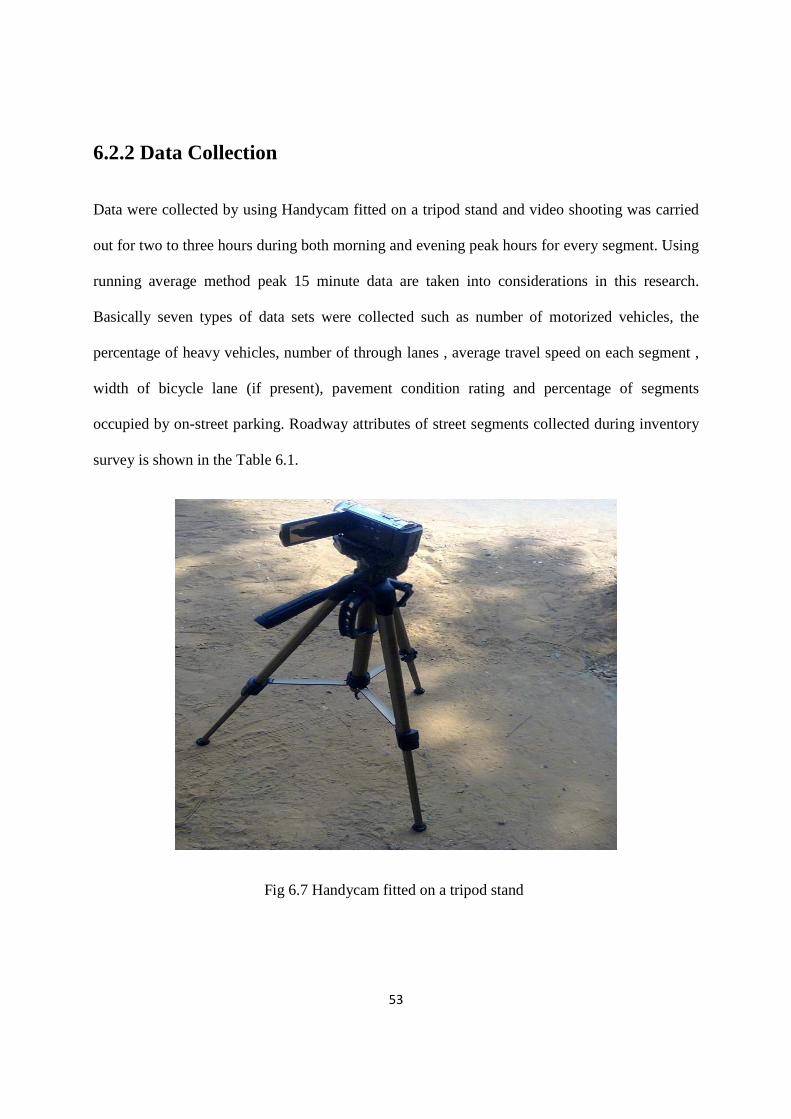
53
6.2.2 Data Collection
Data were collected by using Handycam fitted on a tripod stand and video shooting was carried
out for two to three hours during both morning and evening peak hours for every segment. Using
running average method peak 15 minute data are taken into considerations in this research.
Basically seven types of data sets were collected such as number of motorized vehicles, the
percentage of heavy vehicles, number of through lanes , average travel speed on each segment ,
width of bicycle lane (if present), pavement condition rating and percentage of segments
occupied by on-street parking. Roadway attributes of street segments collected during inventory
survey is shown in the Table 6.1.
Fig 6.7 Handycam fitted on a tripod stand

54
Table 6.1 Roadway attributes of street segments collected during inventory survey
Segment No. ……………………………………………………………………… Segment Name ……………………………………………………………………
Attributes
No. of lanes
No. of vehicles in peak
15minutes
Percentage of heavy vehicles
No. of through lanes
Average travel
speed on street
segments
Bicycle lane
(Yes/No)
Pavement condition
rating (Excellent-5……Bad-
1)
On Street
Parking (%)
Six Lane Divided
540 1 1 40 No 5 0%
Four Lane Divided
280 5 1 40 No 4 1%
Two Lane Undivided
700 7 1 40 No 3 2%
Two Lane Undivided
800 9 1 40 No - 3%
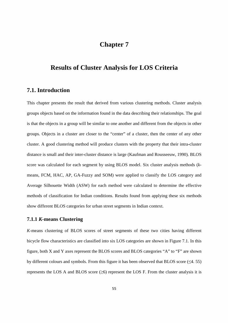
55
Chapter 7
Results of Cluster Analysis for LOS Criteria
7.1. Introduction
This chapter presents the result that derived from various clustering methods. Cluster analysis
groups objects based on the information found in the data describing their relationships. The goal
is that the objects in a group will be similar to one another and different from the objects in other
groups. Objects in a cluster are closer to the “center” of a cluster, then the center of any other
cluster. A good clustering method will produce clusters with the property that their intra-cluster
distance is small and their inter-cluster distance is large (Kaufman and Rousseeuw, 1990). BLOS
score was calculated for each segment by using BLOS model. Six cluster analysis methods (k-
means, FCM, HAC, AP, GA-Fuzzy and SOM) were applied to classify the LOS category and
Average Silhouette Width (ASW) for each method were calculated to determine the effective
methods of classification for Indian conditions. Results found from applying these six methods
show different BLOS categories for urban street segments in Indian context.
7.1.1 K-means Clustering
K-means clustering of BLOS scores of street segments of these two cities having different
bicycle flow characteristics are classified into six LOS categories are shown in Figure 7.1. In this
figure, both X and Y axes represent the BLOS scores and BLOS categories “A” to “F” are shown
by different colours and symbols. From this figure it has been observed that BLOS score (≤4. 55)
represents the LOS A and BLOS score (≥6) represent the LOS F. From the cluster analysis it is
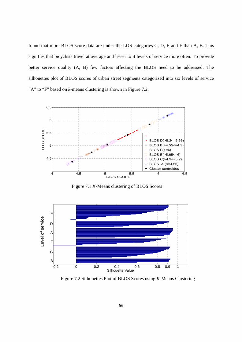
56
found that more BLOS score data are under the LOS categories C, D, E and F than A, B. This
signifies that bicyclists travel at average and lesser to it levels of service more often. To provide
better service quality (A, B) few factors affecting the BLOS need to be addressed. The
silhouettes plot of BLOS scores of urban street segments categorized into six levels of service
“A” to “F” based on k-means clustering is shown in Figure 7.2.
4 4.5 5 5.5 6 6.5
4.5
5
5.5
6
6.5
BLOS SCORE
BLO
S S
CO
RE
BLOS D(>5.2<=5.65)
BLOS B(>4.55<=4.9)
BLOS F(>=6)
BLOS E(>5.65<=6)BLOS C(>4.9<=5.2)
BLOS A (<=4.55)
Cluster centroides
-0.2 0 0.2 0.4 0.6 0.8 0.9 1
E
D
A
F
C
B
Silhouette Value
Leve
l of s
ervi
ce
Figure 7.1 K-Means clustering of BLOS Scores
Figure 7.2 Silhouettes Plot of BLOS Scores using K-Means Clustering

57
From this figure it has been observed that Silhouette values lie between 0.9 and 1.0 for BLOS
categories A and B. Based on this plot, it has been observed that BLOS data of group A and B
are strongly bonded, although data are less in comparison to group C and E. This suggests that
segments providing good quality of services are having very good geometry features (pavement
in good condition, bicyclist get good percentage of shared space) and traffic flow of motorised
vehicles are well managed within the available width of roadways. There lies an average bonding
between the data of group C and D; which indicate that pavement condition of some segments
are good and some segments are below average. Similarly, on some segments traffic movement
is well organized and on some segments traffic move in a very haphazard manner. Bonding
among data sets for LOS E and F are comparatively poor. This is because of large diversity lies
among road segments in terms of road geometry and general operational characteristics of traffic
flow. Also large numbers of road segments are within BLOS categories E and F; which indicate
that a major share of the road network are not bicycle user friendly and need substantial
improvement in this regard.
7.1.2 Hierarchical Agglomerative Clustering (HAC)
Another hard partitioning method such as Hierarchical Agglomerative Clustering (HAC) is used
to classify BLOS scores to find the LOS categories for different urban street segments surveyed
are shown in Figure 7.3. In this method, hierarchical tree of binary clusters was divided into
larger clusters using the cluster function and desired number of groups formed. In this figure,
BLOS scores for six categories “A” to “F” for urban street segments are shown by different
colours and shapes. From this figure it has been observed that BLOS score (≤4. 5) represents the
LOS A and BLOS score (≥5. 85) represent the LOS F. Figure indicate more dense group C, D, E
and F than A, B. Also, data sets under BLOS categories A and B follow shorter ranges compared

58
to others. Traffic on these two better service categories mostly follows more homogeneous flow
with better roadway geometry features. Whereas, traffic flow for other categories are
heterogeneous with varying roadway features makes it more congested to flow by vehicles and
bicyclists. The silhouettes plot for the bicycle score of LOS categories “A” to “F” for urban
street segments based on HAC clustering is shown in Figure 7.4.
4 4.5 5 5.5 6 6.54
4.5
5
5.5
6
6.5
BLOS SCORE
BLO
S S
CO
RE
BLOS E(>5.5<=5.85)
BLOS D(>5.15<=5.5)
BLOS A(<=4.5)
BLOS B(>4.5<=4.75)
BLOS C(>4.75<=5.15)
BLOS F(>=5.85)
-0.4 -0.2 -0 0.2 0.4 0.6 0.8 10.750.7
A
B
E
F
D
C
Silhouette Value
Leve
l of se
rvic
e
Figure 7.3 HAC of BLOS Scores
Figure 7.4 Silhouettes Plot of BLOS Scores using HAC

59
From this figure it has been observed that silhouette values lie between 0.8 and 1.0 for few street
segments of BLOS category A and in maximum cases silhouette values lies between 0.60 and
0.75, indicated by BLOS categories (B-E) and silhouette values lies between 0.4 and 0.70,
indicated by BLOS category F. For the group A, B and C data are well bonded within the same
group than the other groups of data.
Hierarchical tree of binary clusters was divided into larger clusters using the cluster function.
The dendogram formed out of bicycle score data was cut off at a level where it formed six
clusters as shown in Figure 7.5; the dendogram is shown starting from a level where it will have
only 30 leaf nodes. Therefore, in Figure 7.5, some of the leaf nodes among these 30 nodes will
have multiple data points.
4 5 3 18 1 2 6 20 7 9 111415211712101922232629 8 132425162827300
0.2
0.4
0.6
0.8
1
LEAF NODES
DIS
TA
NC
E V
EC
TO
R
Figure 7.5 Dendogram using HAC on bicycle score data
7.1.3 Fuzzy C-Means (FCM) Clustering
Fuzzy clustering generalizes partition clustering methods (such as k-means) by allowing an
individual to be partially classified into more than one cluster. In partition clustering, each

60
individual is a member of only one cluster. Where as in fuzzy clustering objects are not assigned
to a particular cluster: they possess a membership coefficient indicating the strength of
membership in all or some of the clusters. This is called fuzzification of the cluster
configuration. In a fuzzy cluster analysis, the number of subsets is assumed to be known, and the
membership coefficient of each object in each cluster is estimated using an iterative method,
usually a standard optimization technique based on a heuristic objective function. The concept of
a membership coefficient derives from fuzzy logic but the connection between fuzzy logic and
fuzzy cluster analysis is usually only through the application of membership coefficient, and not
the more comprehensive theory.
Fuzzy C-Means (FCM) Clustering is also used for the classification of BLOS scores into
categories. BLOS scores found using BLOS model developed in Indian context are used as the
input values in Fuzzy C-Means (FCM) Clustering for the classification of the service measure
into six categories are shown in Figure 7.6. In this figure, bicycle scores of LOS categories “A”
to “F” for urban street segments are shown by different colours and symbols. From this figure it
has been observed that BLOS score (≤4. 5) represents the LOS A and BLOS score (≥6) represent
the LOS F. The silhouettes plot for the BLOS scores of service categories “A” to “F” of urban
street segments based on Fuzzy C-Means (FCM) clustering is shown in Figure 7.7. From this
figure it has been observed that Silhouette values lie between 0.90 and 1.0 for street segments
under BLOS categories A and B, which indicates that data are well bonded because of similarity
in road features and traffic characteristics. The same characteristics for BLOS categories C, D, E
and F are somewhat varying.

61
4 4.5 5 5.5 6 6.5
4
4.5
5
5.5
6
6.5
BLOS SCORE
BLO
S S
CO
RE
Cluster centroids
BLOS F(>=6)
BLOS A(<=4.5)
BLOS C(>4.9<=5.2)
BLOS B(>4.5<=4.9)
BLOS E(>5.6<=6)
BLOS D(>5.2<=5.6)
-0.2 0 0.2 0.4 0.6 0.8 0.90.95 1
B
A
C
D
F
E
Silhouette Value
Leve
l of s
ervi
ce
Figure 7.6 FCM Clustering of BLOS Scores
Figure 7.7 Silhouettes Plot of BLOS Scores using FCM Clustering

62
7.1.4 Affinity Propagation (AP) clustering
AP which is a new clustering tool developed in the recent past is used to classify the BLOS score
for different urban street to find the ranges of LOS categories. Every algorithm has its natural
way of classification of the data set into number of groups. When a data set is clustered into its
optimal number of clusters the quality of the cluster is best as the variation between the data
points belonging to a particular cluster is minimal. The user selects initial “self similarity” values
from a set derived from the data itself, such that lower self similarity values give rise to a smaller
number of clusters.
BLOS scores of various street segments found by the calibration of BLOS model are given to the
algorithm in the form of similar matrix. The distribution of data after AP clustering is shown in
fig 7.8. The different cluster group represents different LOS categories for urban streets. Where
LOS A represent the best (<=4. 5) and LOS F represent the worst (>=5. 85). From the categories
ranges it is observed that more data are in the LOS categories C,D,E and F than A, B i.e. number
of street segments having more BLOS score are higher. Also level of service ranges are higher
than the ranges provided by FDOT. It indicates that the bicycle level of service in Indian cities is
poorer than the Florida due to scarcity of facility for bicyclists in the roadway environment in
Indian urban context.

63
0 A B C D E F4
4.5
5
5.5
6
6.5
LEVEL OF SERVICE
BLO
S S
CO
RE
BLOS F>=5.85
BLOS E>(5.55-5.85)
BLOS D>(5.16-5.55)
BLOS C>(4.85-5.16)
BLOS B>(4.5-4.85)
BLOS A<=4.5
Figure 7.8 Plot for bicycle LOS for Urban Street segments using Affinity Propagation (AP)
clustering
7.1.5 GA-Fuzzy
Like the previous algorithms input data (BLOS score) to GA-Fuzzy clustering and its output
(cluster centers) found from the cluster analysis are used in computing the values to classify the
input data. In this study data collected from 35 road segments were analyzed using BLOS model
and BLOS score for each segment are classified using GA-Fuzzy algorithm. GA-Fuzzy
algorithm classified BLOS score data of each segment for each direction into six clusters to find
the LOS ranges of different urban street segments. The result of clustering is shown in figure 7.9.
Each LOS class represented in the figure with a different symbol and colour. Legend of the
figure illustrated the ranges of LOS classes (A-F), where LOS A represent the best (<=4. 5) and
LOS F represent the worst (>=6). From the figure it is observed that more data are in LOS group
C, D, E and F (poor) than A, B (good) quality level of service. Because of unplanned lane space
utilization and poor management of traffic in urban Indian context.

64
0 A B C D E F4
4.5
5
5.5
6
6.5
LEVEL OF SERVICE
BLO
S S
CO
RE
BLOS F>=6
BLOS E>(5.6-6)
BLOS D>(5.15-5.6)
BLOS C>(4.9-5.15)
BLOS B>(4.5-4.9)
BLOS A<=4.5
Figure 7.9 Plot for bicycle LOS for Urban Street segments using GA-Fuzzy clustering
7.1.6 SOM in ANN
Similarly SOM algorithm of ANN is also used to classify BLOS score found from BLOS model
for the categorization of LOS ranges. The result of clustering is shown in figure 7.10. Each LOS
class represented in the figure with a different symbol and colour and ranges (A-F), where LOS
A represent the best (<=4. 85) and LOS F represent the worst (>=6). In this clustering method
data points of group A are more than the other clustering methods which indicates SOM method
consider relatively more number of good qualities of street segments than the other methods, but
like the other methods the figure represents more data points in group D, E and F than A,B and
the separation between the data points of group A are higher than the other group indicates not
properly bonded.

65
0 A B C D E F4
4.5
5
5.5
6
6.5
LEVEL OF SERVICE
BLO
S S
CO
RE
BLOS F>=6
BLOS E>(5.65-6)
BLOS D>(5.4-5.65)
BLOS C>(5-5.4)
BLOS B>(4.85-5)
BLOS A<=4.85
Figure 7.10 Plot for bicycle LOS for Urban Street segments using SOM clustering
K-means, HAC, FCM, AP, GA-Fuzzy and SOM clustering methods are used to classify BLOS
scores to find LOS ranges. Values of LOS ranges of six methods are different from one to
another as represented in Table 3. The lowest value represents BLOS A, i.e. the compatibility
level is extremely high and the highest value represents BLOS F, i.e. the compatibility level is
extremely low. From different plots of various clustering methods it is interpreted that poor
service quality (D, E, and F) follow the road segments more often than good quality of service
(A, B, C). To full fill the objective of the study i.e. to know the best clustering method suitable to
define BLOS criteria in Indian context, Average Silhouettes Width (ASW) for all these six
clustering methods are calculated. From the calculated ASW, it is observed that K-means, HAC,
FCM, AP, GA-Fuzzy and SOM clustering methods have ASW values 0.7263, 0.604, 0.7167,
0.571, 0.564 and 0.465 respectively. Table 7.1 represents various BLOS ranges derived from
various clustering method and ASW of these used methods.

66
Table 7.1 Classification of scores to define BLOS categories in Indian context
BLOS K-means
Clustering
Hierarchical Agglomerative
Clustering (HAC)
Fuzzy C-Means (FCM)
Clustering
Affinity Propagation
(AP) clustering
GA-Fuzzy
Self
Organizing
Map
(SOM)
A ≤4.55 ≤4.5 ≤4.5 ≤4.5 ≤4.5 ≤4.85 B >4.55≤4.9 >4.5≤4.75 >4.5≤4.9 >4.5≤4.85 >4.5≤4.9 >4.85≤5 C >4.9≤5.2 >4.75≤5.15 >4.9≤5.2 >4.85≤5.16 >4.9≤5.16 >5≤5.4
D >5.2≤5.65 >5.15≤5.5 >5.2≤5.6 >5.16≤5.55 >5.16≤5.6 >5.4≤5.65
E >5.65≤6 >5.5≤5.85 >5.6≤6 >5.55≤5.85 >5.6≤6 >5.65≤6 F ≥6 ≥5.85 ≥6 ≥5.85 ≥6 ≥6
Average Silhouette
Width ASW
0.7263 0.604 0.7167 0.571 0.564 0.465
Various ranges of Average Silhouette Width are presented in table 7.2 indicate the strength and
weakness of the structure.
Table 7.2 Ranges of ASW (Source: Kaufman & Roosseeuw 1990, chapter 2, pp. 88)
ASW of various used clustering methods is different from one to another and compared as
shown in figure 7.11.
I 0.71-1.00 A strong structure has been found
II 0.51-0.70 A reasonable structure has been found
III 0.26-0.50 The structure is weak and could be artificial
IV ≤ 0.25 No substantial structure has been found

67
Figure 7.11 Comparison of ASW values of various clustering methods
According to Kaufman & Roosseeuw (1990) more the ASW value represents a strong structure.
K-means and FCM have the ASW ranges in between 0.71-1.0 (strong structure), HAC, AP and
GA-fuzzy have the ASW ranges in between 0.51-0.70 (reasonable structure) and SOM has the
ASW ranges in between 0.26-0.50 (weak structure). Science K-means clustering has the highest
average silhouette width than the other five clustering methods, K-means is a more suitable
method to classify BLOS score of urban on street road segments in Indian context. BLOS score
ranges of each individual level of service category using K-means clustering are elaborated in
Table 7.3. From the table it can be outlined that level of service ranges are higher than the ranges
provided by FDOT.

68
Table 7.3 Comparison of BLOS ranges in Indian context with FDOT BLOS ranges
BLOS K-MEAN CLUSTERING
BLOS RANGES FDOT BLOS RANGES
A ≤4.55 ≤ 1.5 B >4.55≤4.9 > 1.5 and ≤ 2.5 C >4.9≤5.2 > 2.5 and ≤ 3.5 D >5.2≤5.65 > 3.5 and ≤ 4.5 E >5.65≤6 > 4.5 and ≤ 5.5 F ≥6 > 5.5

69
Chapter 8
Summary, Conclusions and Future Scope
8.1 Summary
In this study, an attempt has been made to define bicycle LOS criteria for urban on-streets in the
context of Indian cities. Handycam was used to collect data from different street segments.
Various methods of bicycle LOS analysis are discussed in the literature review. From literatures
it is observed that BLOS model developed by FDOT is in a very generic form, the coefficients of
which can be easily calibrated in Indian context. BLOS model associate with several factors
from which average effective width of the outside through lane, motorized vehicle volumes,
motorized vehicle speeds, percentage of heavy vehicles (truck) and pavement condition rating
have significant effect whereas bicycle volumes and pedestrian volumes have insignificant effect
on BLOS. From all these factors “effective width of outside through lane” affect the most to
BLOS score. Many researchers have adopted this model to define LOS in different countries and
some have adopted Bicycle Compatibility Index (BCI) model. Based on safety point of view
various models were developed such as Bicycle Safety Index Rating (BSIR), roadway condition
index (RCI), Intersection Hazard Score (IHS), and Intersection Safety Index (ISI).
Defining BLOS is basically a classification problem and cluster analysis is found to be the most
suitable technique for solving this classification problem. Cluster analysis groups objects based
on the information found in the data describing their relationships. K-means, hierarchical
agglomerative, fuzzy c-means, Affinity Propagation (AP), SOM and GA-fuzzy clustering are the

70
six methods, those are employed to define LOS criteria in this study. The validation parameter,
“silhouette” is used to evaluate and compare partitions resulting from different clustering
algorithms and resulting from the same algorithms under different parameters. ASW is
calculated for every clustering method to compare between the clustering methods and to find
the best clustering method. K-mean cluster analysis is found to be the most suitable method in
defining BLOS ranges for level of service categories of urban streets in Indian context.
8.2Conclusion
Following are the important conclusions that are drawn from the present study in defining
Bicycle level of service criteria for urban streets in Indian context.
� The BLOS model which is calibrated for Indian context having lower coefficient values
for a1, a2, a3 and higher value for a4 than BLOS model developed by FDOT 2009.
� It is observed that the numbers of motorized vehicles, vehicular speed and percentage of
heavy vehicles have a negative impact and width of outside through lane, pavement
condition rating have a positive impact on bicycle LOS.
� Bicycle LOS on urban on-streets are defined based on BLOS scores used by six cluster
analysis methods. Defined BLOS scores for LOS categories are found to be different for
all six clustering methods. BLOS score ranges for LOS categories (A-F) in the present
study are found to be higher (implies lower in BLOS) than the ranges provided by FDOT
(2009). The poor in service quality are due to the absence of separate bicycle lane, highly
heterogeneous traffic flow on urban road corridors with varying geometry in India.
� Due to higher in Average Silhouettes Width (ASW) K-means is perceived to be better to
classify BLOS score data than the other five clustering methods applied in this study.

71
� Also, it was found that bicycle traveled, more often, at the poor quality of service of “D”,
“E” and “F”, than good quality of service of “A”, “B” and “C”.
8.3 Contributions
Bicycle level of service ranges for level of service categories of urban streets are defined using
cluster analysis methods and BLOS model is calibrated and co-efficients are changed
considering the local conditions of road segments for the first time in Indian context.
8.4Applications
BLOS assessment may be functional in several ways:
The bicycle level of service categories (A-F) defined in this study can be used in general in the
bicycle level of service analysis of urban streets in Indian context which will help to the
transportation planner and designer for a bicycle friendly environment. A bicycle map can be
produced to attract bicyclist and a pollution free environment can be predicted.
8.5 Limitations and Future Scope
There are opportunities for further improvement to this study. Some of them are given below:
The study area for the present study was confined to two cities in India due to time and budget
constraints. Similar study needs to be carried out in a number of cities in India. As one calibrated
model and six clustering methods, are used for this study, there are opportunities for calibration
of various models such as BCI, BSIR and ISI using the field data and use of various clustering
methods for defining LOS criteria of bicycle in urban Indian context. In this study BLOS scores
72
are calculated only for on street segments, similar research needs to be carried out for signalized
intersections and off-street bicycle facilities.
The model is not applicable to off-street bicycle facilities, such as shared use paths or sidewalks.
This study is a quantitative analysis of bicycle level of service but bicyclist perception of existing
facility should be paid due consideration while defining bicycle level of service criteria of urban
streets. In true sense to make the methodology on bicycle level of service analysis more realistic
stated preference survey of bicyclist needs to be conducted and analyzed. However, the structure
of the combined methodology on bicycle level of service analysis using quantitative and
qualitative methods needs a thorough research.
73
References
Bezdek, J. C. Pattern recognition with fuzzy objective function algorithm. Plenum, New York.
1981.
Bezdek, J. C. Keller, J. M. Krishnapuram, R. and Pal, N. R. Fuzzy models and algorithms for
pattern recognition and image processing, Kluwer Academic Pub., Norway.1999.
Bhuyan, P. K., Rao, K.V. K. Defining los criteria of Urban Streets using GPS data: k-means and
k-medoid clustering in Indian context., Transport, Taylor and Francis, Vol. 27 (2), 2012, pp.
149-157.
Bhuyan ,P. K., Rao, K.V. K. Defining Level of Service Criteria of urban Streets in Indian
Context. European Transport, Issue 49, 2011, pp. 38-52.
Bhuyan, P.K., Rao K.V.K. FCM Clustering Using GPS Data for Defining Level of Service
Criteria of Urban Streets. Transport Problems: an International Scientific Journal, Poland, Vol.
5 (4), 2010, pp. 105-113.
Botma, H. Method to Determine Level of Service for Bicycle Paths and Pedestrian- Bicycle
Path. Transportation Research Record, 1502, Transportation Research Board, Washington, D.C.
1995.

74
Carter , D.L., Hunter, W.W., Zegeer, C.V., Stewart, J.R., Huang, H. Bicyclist Intersection Safety
Index. 86th annual meeting of the Transportation Research Board , National Research Council,
Washington, D.C. 2007, pp. 1–16.
Crider, L., Burden, J. Han, F. Multimodal los point level of service project. Gainesville, Florida.
http://www11.myflorida.com/planning/systems/sm/los/pdfs/pointlos.pdf, 2001.
Davis, J. Bicycle Safety Evaluation. Auburn University, City of Chattanooga, and Chattanooga-
Hamilton County Regional Planning Commission, TN, 1987.
Dixon, L. B. Bicycle and Pedestrian Level-of-Service Performance Measures and Standards for
Congestion Management Systems. Transportation Research Record, 1538, Transportation
Research Board, Washington, D.C. 1996, pp. 1-9.
Dougald, L.E., Dittberner, R.A., Sripathi,H.K. Creating safer mid-block pedestrian and bicycle
crossing environments: The zig-zag pavement marking experiment. Annual meeting of the
Transportation Research Board, Washington, D.C., 2012, pp. 1–18.
Dowling, R., Reinke, D., Flannery, A., Ryus, P., Vandehey, M., Petritsch, T., Landis.,
Rouphail,N. Bonneson, J. Multimodal Level of Service Analysis for Urban Streets, NCHRP
report 616, Transportation Research Board, Washington D.C. 2008.

75
Dowling, R., Flannery, A., Landis, B., Petritsch, T., Rouphail, N., Ryus, P. Multimodal Level of
Service Analysis for Urban Streets, Transportation Research Reecord, 2071, Transportation
Research Board , Washington, D.C., 2008, pp1-7.
Duthie, J., Brady, J. F., Mills, A. F., Machemehl, R. B. Effects of On-Street Bicycle Facility
Configuration on Bicyclist and Motorist Behavior. Transportation Research Record, 2190,
Transportation Research Board , Washington, D.C., 2010 , pp. 37-44.
Elias. A. Automobile-Oriented or Complete Street? Pedestrian and Bicycle Level of Service in
the New Multimodal Paradigm. Transportation Research Record, 2257, Transportation Research
Board Washington, D.C., 2011, pp. 80–86.
Epperson, B. Evaluating the Suitability of Roadways for Bicycle Use: Towards a Cycling Level
of Service. Transportation Research Record, 1438. Transportation Research Board, Washington,
DC. 1994.
FDOT, Quality/Level of service handbook. Department of Transportation. State of Florida.
2002.
FDOT, Quality/Level of service handbook. Department of Transportation. State of Florida.
2009.

76
FHWA. The Bicycle Compatibility Index: A Level of Service Concept, Implementation Manual.
Federal Highway Administration, FHWA- RD-98-095, Washington, DC. 1998.
Frey, B. J., Dueck, D. Clustering by passing messages between data points. Science, 315 (5814),
2007, pp. 972–976.
Fukunaga, K. Introduction to statistical pattern recognition. Academic Press, San Diego, CA.
1990.
Guttenplan, Landis, Crider L., McLeod, S.D. Multimodal Level-of-Service Analysis at Planning
Level. Transportation Research Record, 1776, Transportation Research Board, Washington,
D.C., 2001, pp. 151-158.
Harkey, D.L., Reinfurt, D.W., Knuiman, M., Stewart, J.R., Sorton, A., Development of the
Bicycle Compatibility Index: A Level of Service Concept. Federal Highway Administration,
FHWA-RD-98-072., McLean, VA. 1998.
Heinen, E., Maat, K. Are longitudinal data unavoidable? Measuring variation in bicycle mode
choice. 91st annual meeting of the Transportation Research Board, National Research Council,
Washington, D.C., 2012 pp. 1–21.
Highway Capacity Manual. Transportation Research Board, 2000, Washington, D.C.

77
Highway Capacity Manual. Transportation Research Board, 2010, Washington, D.C.
Hunter, W. W., Stewart, J. R., Stutts, J. C. Study of Bicycle Lanes Versus Wide Curb Lanes.
Transportation Research Record, 1674, Transportation Research Board, Washington, D.C.,
1999.
Jain, A.K., Dubes, R.C. Algorithms for clustering data, Prentice Hall, Englewood Cliffs, 1988.
Jensen, S. U. Pedestrian Bicycle Level of Service on Roadway Segments. Transportation
Research Record, 2031, Transportation Research Board , Washington, D.C., 2007, pp. 1-17.
Kaufman, L., Rousseeuw, P. J. Finding groups in data: An introduction to cluster analysis,
Wiley, New York, 1990.
Kendrick, C. M., Moore, A., Haire, A., Bigazzi, A., Figliozzi, M., Monsere,C.M., George,L.
Impact of Bicycle Lane Characteristics on Exposure of Bicyclists to Traffic-Related Particulate
Matter. Transportation Research Record, 2247, Transportation Research Board, Washington,
D.C., 2011, pp. 24–32.
Kidarsa, R., Pande, T., Vanjari, S. V., Krogmeier, J. V., Bullock Design Considerations for
Detecting Bicycles with Inductive Loop Detectors. Transportation Research Record,. 1978,
Transportation Research Board, Washington, D.C., 2006, pp. 1-7.

78
LaMondia, J. J, Duthie,J. C. An Ordered Probit Regression Analysis of Factors Influencing
Bicycle-Vehicle Interactions on Urban Roadways. 91st annual meeting of the Transportation
Research Board, Washington, D.C., 2012, pp. 1–20.
Landis, B. W. Bicycle Interaction Hazard Score: A Theoretical Model.” Transportation
Research Record ,1438, Transportation Research Board, Washington, DC.1994.
Landis, B. W., Vattikuti, V. R., Ottenberg, R. M., Petritsch, T. A, Guttenplan, M., Crider, L. B.
Intersection Level of Service for the Bicycle Through Movement. Transportation Research
Record, 1828, Transportation Research Board, Washington, D.C., 2003, pp. 101-106.
Landis, B. W., Vattikuti, V. R. Brannick , M. T. Real-Time Human Perceptions Toward a
Bicycle Level of Service. Transportation Research Record, 1578, Transportation Research
Board, Washington , D.C., 1997, pp. 119-126.
Li, Z., Wang, W., Liu, P., Schneider, R. Ragland, D.R. Investigating Bicyclists’ Perception of
Comfort on Physically Separated Bicycle Paths: An Examination based on Survey Data in China.
91st annual meeting of the Transportation Research Board, Washington, D.C., 2012. pp. 1–23.
Lowry, M. B., Callister, D., Gresham, M., Moore, B. Using Bicycle Level of Service to Assess
Community-wide Bikeability. 91st annual meeting of the Transportation Research Board,
Washington, D.C., 2012, pp. 1–15.

79
Monsere, C. M., McNeil, N., Dill, J. Multi-User Perspectives on Separated, On-Street Bicycle
Infrastructure. 91th annual meeting of the Transportation Research Board, Washington, D.C.,
2012, pp. 1–14.
Niemeier, D. A. Longitudinal analysis of bicycle count variability: results and modeling
implications” Transportation Engineering, ASCE 122 (3), 1998.pp. 200-206.
Petritsch, T. A., Landis, B. W., Huang, H. F., McLeod, P.S. Bicycle Level of Service for
Arterials. annual meeting of the Transportation Research Board, National Research Council,
Washington, D.C., 2007, pp. 1–22.
Robertson, J. A. A Traffic Operations Method for Assessing Automobile and Bicycle Shared
Roadways, Submitted to the Office of Graduate Studies Texas A&M University, 2010. pp.1-13.
Rousseeuw, P. J. Silhouettes: A graphical aid to the interpretation and validation of cluster
analysis. J. Comput. Appl. Math., 20, 1987. pp. 53-65.
Sayed, T. Abdelwahad, W., Navin, F. Identifying accident prone locations using fuzzy pattern
recognition. Journal of Transportation Engineering, ASCE, 121(4), 1995, pp. 352–358.
Seiichi, A., Katia, K.,Investigating active cyclists’ behavior: Influencing factors on commuting
by bicycle. 91st annual meeting of the Transportation Research Board, Washington, D.C., 2012,
pp. 1–14.

80
Sorton, A. Thomas , W. Bicycle Stress Level as a Tool to Evaluate Urban and Suburban Bicycle
Compatibility. Transportation Research Record, 1438. Transportation Research Board,
Washington, DC. 1994.
Sprinkle Consulting Lnc. (SCI), Bicycle level of service: Applied model. Tampa, F L. 2007.
Torbic, D., Elefteriadou, L., El-Gindy, M. Development of Rumble Strip Configurations That
Are More Bicycle Friendly. Transportation Research Record, 1773, Transportation Research
Board, Washington, D.C., 2001.pp. 23-31.
Turner, S., Shafer, C. S., Stewart, W. P. Bicycle suitability criteria: literature review and state-of-
the-practice survey. 1997.
Wang, X. L. A course in fuzzy systems and control, Prentice-Hall International, Upper Saddle
River, New Jersey. 1997.
Yang, C., Wang, W., Shan, X., Jin, J., Lu, J. Li, Z. Effects of Personal Factors on Bicycle
Commuting in Developing Countries: Case Study of Nanjing, China. Transportation Research
Record, 2193, Transportation Research Board, Washington, D.C., 2010, pp. 96–104.
Zolnik, E. J., Cromley, E. K. A Poission-multilevel, bicycle level-of-service methodology for
rural road networks. 86th annual meeting of the Transportation Research Board, National
Research Council, Washington, D.C., 2006. pp. 1–13.

81
List of Publications
Journals: published
1. Bhuyan, P. K, Nayak, M. S. A Review on Level of Service Analysis of Urban Streets.
Transport reviews, Vol. 33, No. 2, 2013, 219–238.
Submitted
2. Nayak, M. S., Bhuyan, P.K. Bicycle Level of Service in Urban Indian Context. Transport
policy, 2013.
Under Preparation
3. Nayak, M. S., Bhuyan, P.K. Defining BLOS Criteria of Urban on Street Road Segments Using
SOM, GA-Fuzzy and AP Clustering in Indian Context. Transportation, 2013.