Beyond-the-Standard-Model Contributions to Rare B Decays Analyzed with Variational-Bayes Enhanced Adaptive Importance Sampling

Master's thesis

Stephan JahnFebruary 2015

AbstractWe propose an algorithm that automatically finds a Gaussian mixture to be used as proposal density for importance sampling. The algorithm uses Markov chains to find regions of interest and the variational-Bayes approach to fit a Gaussian mixture. We provide an open-source implementation in the python package pypmc. This work improves the algorithm developed by Frederik Beaujean (2012) in the sense that the enhanced algorithm needs fewer function evaluations to produce equivalent results. In the future, the algorithm can be stabilized with our extension of the variational-Bayes approach in the context of Student's T mixture densities. We apply the Gaussian version of our algorithm to constrain the effective couplings in an effective theory governing b→ s quark transitions. Our analysis of the scalar, pseudoscalar, and tensor Wilson coefficients requires sampling and numerical integration of a multimodal, 37 dimensional function. The combined experimental constraints on the B →K μ

+μ

− angular decay distribution and the branching ratios of B s→μ

+μ

− and B →K *μ

+μ

− can simultaneously constrain all Wilson coefficients mentioned above. We find that the standard model is in good agreement with the data acquired during the last LHC run.

Contents1 Introduction 1

2 Probability theory 42.1 Basics........................................................................................................42.2 Bayes' theorem.........................................................................................52.3 Law of large numbers..............................................................................6

3 Variational Bayes 83.1 Basics........................................................................................................83.2 Gaussian mixture...................................................................................103.3 Student's T mixture................................................................................13

3.3.1 Framework...............................................................................................143.3.2 Conjugate prior for the degrees of freedom............................................20

4 Monte Carlo sampling methods 224.1 Markov chains.........................................................................................224.2 Importance sampling.............................................................................24

4.2.1 Basics......................................................................................................244.2.2 Adaptive importance sampling................................................................25

5 Importance sampling initialized with Markov chains 295.1 Markov chain prerun..............................................................................305.2 First Proposal for importance sampling..............................................30

5.2.1 Hierarchical clustering.............................................................................315.2.2 Population Monte Carlo...........................................................................325.2.3 Variational Bayes.....................................................................................335.2.4 Discussion................................................................................................35

5.3 Further proposal updates......................................................................435.3.1 Original algorithm.....................................................................................435.3.2 Enhanced algorithm.................................................................................445.3.3 Discussion................................................................................................46

5.4 Final run..................................................................................................47

6 Bayesian analysis of new physics in rare B decays 486.1 Theory of rare B decays........................................................................486.2 Methodology...........................................................................................51

6.2.1 Experimental constraints.........................................................................536.2.2 Parameters and priors.............................................................................54

6.3 Results and discussion.........................................................................566.4 Sampling performance..........................................................................62

7 Conclusion 65

A Probability Distributions 67A.1 Gauss / Normal.......................................................................................67A.2 Student's T..............................................................................................67

A.3 Gamma....................................................................................................68A.4 Log-gamma.............................................................................................68A.5 Dirichlet...................................................................................................69A.6 Wishart....................................................................................................70A.7 Normal-Wishart.......................................................................................70

B The python package pypmc 71

C Supplement to chapter 6 71C.1 The HPQCD form factor constraint.......................................................71C.2 Wilson coefficients – SM prediction.....................................................73C.3 Internal EOS report................................................................................73

List of abbreviations 77

Bibliography 78

Acknowledgments 86

1 IntroductionThe standard model (SM) of particle physics was recently celebrated for its latest success, the discovery of the last missing particle - the Higgs boson [ATLAS12] [CMS12] [EB64] [Hig64] [GHK64]. However, several unsolved questions and unexplained phenomena remain. Neutrino masses [BM14] and dark matter [Tri87] are only two of them. Plenty of SM extensions have been proposed in an attempt to solve the remaining problems. Many (e.g. supersymmetry [Mar11]) predict new elementary particles.There are in principle two methods to look for new particles: Direct and indirect searches. In a direct search, one tries to produce one or more new elementary particles on shell as part of the final state of a high-energy collision. So far, only SM particles have been seen at colliders such as the LHC.We only consider the indirect search via flavor physics here. In the standard model, flavor changing processes can only be mediated by the charged W± bosons. Thus, SM flavor-changing neutral currents (FCNCs) first occur at one-loop level in perturbation theory. Particles beyond the SM may manifest themselves as additional particles that run in the loop. There is a good chance to find new physics in FCNC observables since we can hope for new physics contributions that enter at the same order as SM contributions. In particular, rare decays of B mesons (mesons with b quark content) are candidates to find new physics because SM contributions exhibit further suppression [Bea12]. In this thesis, we consider B decays, where the b quark turns into an s quark and where a lepton-antilepton pair ℓ+ ℓ− is emitted.In order to account for new physics in a model-independent way, B physics is commonly discussed in an effective field theory (EFT) framework (cf. chapter 6.1). In an EFT, all physics at energy scales above the b -quark scale is reduced to effective couplings - the Wilson coefficients C i . On the one hand, the Wilson coefficients can be calculated from a concrete high-energy theory (like the SM) in a procedure called “matching”. On the other hand, the Wilson coefficients can be regarded as numerical values to be extracted from experimental data.Currently, there is special interest in B physics since LHCb recently reported a sizable deviation from the SM in one of the B0

→K *0ℓ+ ℓ− optimized observables [LHC13A]. Descotes-Genon et al. [DMV13] claim large deviations from the standard model in C 7 and C 9 . However, other authors [BBD14] [JC14] comment that the theory uncertainties may be underestimated.In this thesis, we use recent measurements of the muonic (ℓ=μ) B s→μ

+μ

− and B→K (*)

μ+μ

− observables (cf. chapter 6) to fit the (pseudo)scalar and tensor Wilson coefficients. The chosen observables are particularly sensitive to the aforementioned Wilson coefficients. We derive more stringent constraints and compare them to the SM.

The treatment of uncertainties is achieved in a natural way by the Bayesian approach. We account for theory uncertainties by the introduction of so-called nuisance parameters. Our Bayesian analysis yields a posterior distribution that is not analytically tractable and high (30-40) dimensional. More elaborate theoretical treatment may lead to more parameters (dimensions) in the future. We consequently need sophisticated algorithms that at least partially overcome the “curse of dimensionality”. Discrete approximate symmetries, for example C i→−Ci , often lead to a multimodal posterior. Well established algorithms fail because of high dimensionality (e.g. grid-based methods) or multimodality (e.g. Markov chain Monte Carlo).

1

In order to compare different models in a Bayesian framework, we are required to numerically integrate the posterior. As a consequence, we need an algorithm that can compute integrals of multimodal nonnegative functions and that still works in O(40) dimensions. Parallel algorithms are desirable since parallelization is the only way to profit from computing clusters and the next generations of processors. The number of calls to the posterior should, in our application, be kept at a minimum. A single call to the posterior distribution of the Wilson coefficients takes a few seconds.

The challenges described above are typical for Bayesian analyses. Sampling and numerical integration in high dimensions are still unsolved problems. There is no standard algorithm that tackles all of the above mentioned difficulties yet. This thesis is therefore focused on the development of such an algorithm.For unimodal distributions, Hamiltonian (originally: hybrid) Monte Carlo (HMC) [DKPR87] is probably the most efficient known sampling algorithm. It is based on the famous Metropolis-Hastings algorithm [Met+53] [Has70] combined with a sophisticated proposal. However, HMC requires that the target is differentiable and it needs the full gradient as a callable function. Since our targets are multimodal and we do not have access to their gradients1, we cannot use HMC. Besides, it only samples the target but it does not compute the integral. A promising approach to compute integrals is nested sampling [Ski06], where the target is sampled under constraints. A very recent integration approach is proposed by Caldwell and Liu [CL14]. Their trick is to compute the integral only in a subvolume and extrapolate to the entire parameter space. Unfortunately, none of these approaches is applicable for our kind of problem.Importance sampling (cf. chapter 4.2.1) is a promising tool for our purposes. It can cope with multimodal distributions and is trivially parallelized. However, it only works reasonably in high dimensions if the proposal density is not too different from the target distribution. Adaptive importance sampling [Cap+08] [Kil+09] (see also chapter 4.2.2) uses previously obtained samples to improve an existing proposal but this again only works well if the first proposal is not too bad. The question how to find a good first proposal is answered by [Bea12] [BC13]. They suggest to first run local-random-walk Markov chains (cf. chapter 4.1) that just need a moderate initialization. Then, they use the Markov chain samples to generate a proposal for importance sampling. However, the user has to carefully tune many parameters by hand. In addition, a lot of samples are drawn but only used once for a single proposal update.In chapter 5, we present several ways to improve their approach. Our goal is an algorithm that draws samples from an arbitrary function with as few calls to the target function as possible. The results should be robust even with poor parameter input by the user. To approach this goal, we suggest a more efficient usage of population Monte Carlo (PMC) than presented in [Cap+08] and [Kil+09]. Moreover, we incorporate a method suggested by Cornuet et al. [Cor+12] to combine the importance samples from multiple proposals. We further suggest to use the variational-Bayes (VB) method (cf. chapter 3) instead of PMC. We show that VB with Gaussian mixtures is robust against a poor initialization. Last but not least, we provide an extension to existing variational-Bayes approaches with Student's T mixture densities. Because of the heavier tail, we hope that replacing the Gaussian for Student's T distribution reduces outliers (see chapter 4.5 in [Bea12]) and therefore increases the quality of the importance samples.

1 The analytical gradient is not calculated yet and the finite differences method would be far too expensive.

2

The outline of this thesis is as follows: In chapter 2, we review the most important definitions and theorems of probability theory. Chapters 3.1 and 3.2 contain reviews of the general variational-Bayes approach and the specific case with Gaussian mixtures. We extend existing work on the variational-Bayes method with Student's T mixtures in chapter 3.3. Well established sampling algorithms are briefly reviewed in chapter 4. The main work is summarized in chapter 5. There, we present and compare different algorithms that can be used to automatically generate meaningful importance samples. In addition to the toy problems in chapter 5, we also apply the newly developed algorithm to search for new physics in rare B decays in chapter 6.

3

2 Probability theoryWe explain the most important concepts of probability theory in this chapter. Our discussion is restricted to definitions and statements needed in other chapters of this thesis. Useful textbooks for further reading include [Koc07], [Jam06], or [JB03]. The modern axiomatic probability theory is based on a book by Kolmogorov published in 1933 [Kol33].

2.1 Basics

Definition: Probability

Let Ω denote some set (the “sample space”) and ℘(Ω) its power set. The mapping2 P:℘(Ω)→ℝ is called probability if and only if

Axiom 1 P(Ω)=1 (normalization)Axiom 2 ∀ A∈℘(Ω): P( A)≥0 (positivity)Axiom 3 If {An}n∈ℕ is a sequence of mutually exclusive sets (∀ i≠ j : A i∩ A j=∅) then

P(∪n∈ℕ

An)=∑n∈ℕ

P (An) ( σ -additivity).

~

If we set An=∅ ∀n≥N for some finite N ∈ℕ , the finite sum rule is implied by axiom 3.A variable that is connected to the sample space by some function y=f (x ), x∈Ω is called a random variable. If P( y ) is the sampling probability of y , we say “ y is distributed according to P “, y∼P .We denote the joint probability of A and B by P( A ,B)≡P (A∩B) . The conditional probability of A given B is denoted as P( A∣B) and defined by

P( A∣B)≡P( A ,B)

P(B). (1)

The definition of conditional probability gives rise to two important theorems, the law of total probability and Bayes' theorem.

Theorem: Law of total probability

Let {Bn} be a finite or countable partition of Ω ; i.e. the Bn are mutually exclusive and

∪n∈ℕ

Bn=Ω . Then for all A ,C∈℘(Ω)

P( A∣C)=∑n

P (A∣Bn ,C) P(Bn∣C) . (2)

~2 To be precise, P is defined on Z⊆P (Ω) where Z is a σ -algebra. We do not delve into these

mathematical details here.

4

We often consider continuous random variables and a continuous sample space Ω⊆ℝn . It

can be shown that for a nonnegative function p:Ω→ℝ0+ with ∫Ω

p=1 , the integral

P( A)≡∫Ap (x)d x , where A⊆Ω , defines a probability. The function p is called the

probability density function (PDF). The law of total probability,

p(x∣z )=∫ p(x∣y , z ) p ( y∣z )d y , (3)

also holds for PDFs. It is often assumed to be clear from the context, whether a symbol denotes a probability or a probability density.

2.2 Bayes' theorem

Theorem: Bayes' theorem

P(θ∣D , M )=P(D∣θ , M )P(θ∣M )

P(D∣M )(4)

~

Bayes' theorem is the basis of our analysis in chapter 6. It describes how to invert a conditional probability; i.e. it describes how to calculate P(θ∣D , M ) when P(D∣θ , M ) is known. The probability P(D∣θ , M ) is called “likelihood”. It is the sampling probability of a particular data set D , given a model M and model parameters θ . The probability P(θ∣M ) is called “prior”. It describes the knowledge about the parameters θ before

looking at the data. The left hand side of (4) is called the “posterior”. It describes the knowledge about the model parameters θ after we have seen the data D . The denominator Z≡P (D∣M ) is called “evidence”. Using the law of total probability (3), the evidence

Z≡P (D∣M )=∫ dθ P(D∣θ ,M )P (θ∣M) (5)

turns out to be the integral of the numerator. As long as only one model M is considered, the evidence is just an unimportant normalization constant. However, if there are multiple models, the evidence plays a key role in model comparison. Suppose we have two different models that describe the data generating process; i.e. the two likelihoods P(D∣θi , M i) , i=1,2 . We specify the priors P(θi∣M i) , i=1,2 and then make an experiment

that generates data D . What we would like to know is P(M i∣D), i=1,2 , the probability of model i given the data D . Bayes' theorem states

P(M i∣D)=P(D∣M i)P(M i)

P(D)

P(M 1∣D)

P(M 2∣D)=

P(D∣M 1)

P(D∣M 2)⋅

P(M 1)

P(M 2)≡

Z1

Z2

⋅P(M 1)

P(M 2)

. (6)

Note that the probability P(M i∣D) is only defined for the models M 1 and M 2 . It is therefore NOT the absolute probability of model i . It rather is the probability of model i

5

among the other considered models. If there is just one model, P(M∣D ) is always equal to one. It is therefore more useful to consider the ratio

P(M i∣D)=P(D∣M i)P(M i)

P(D)

P(M 1∣D)

P(M 2∣D)=

P(D∣M 1)

P(D∣M 2)⋅

P(M 1)

P(M 2)≡

Z1

Z2

⋅P(M 1)

P(M 2). (7)

The ratio Z1/ Z2 is called Bayes factor, the ratio of the priors is called the prior odds. If no model is preferred a priori ( P(M 1)=P(M 2)) , the Bayes factor Z1/ Z2 is equal to the posterior odds P(M 1∣D )/P( M2∣D ) . A Bayes factor larger than one means that the data prefer model one, a Bayes factor smaller than one means that model two is preferred.

2.3 Law of large numbers

The most important statements in probability theory are “expectation values” (also called “mean values”). As the name suggests, the expectation value describes the expected (more precisely “average”) outcome of a random experiment. By the law of large numbers, the expectation value is equal to the average over many events. The standard deviation estimates how much the samples scatter around the expectation value.

Definition: Expectation value, (co-)variance and standard deviation

Let P be the PDF of a continuous random variable x . Then the integral EP[x ]≡E[ x ]≡∫ x P (x)d x is called the expectation value of x .

The expectation value var (x)≡E [(x−E [x ])2 ] =

simple calculationE[ x2

]−E [x ]2 is called variance

and √var (x ) is called standard deviation of x .For two random variables x and y , cov (x , y)≡E [(x−E [x ])( y−E [ y])] defines the covariance between x and y .

~

Two random variables x and y are called independent if and only if P(x∣y)=P (x) and P( y∣x)=P ( y) . x and y are called uncorrelated if and only if cov (x , y)=0 . Independent

random variables are always uncorrelated but uncorrelated random variables are not necessarily independent.The likelihood (and therefore the posterior) is often only available as computer code. In that case, the only way we can deal with the posterior is a finite number of “samples”. The law of large numbers ensures that we can at least approximate the expectation values of interest with them.

Theorem: Strong law of large numbers

Let {xn} be a sequence of independent and identically distributed (iid) samples (that is the xn are independent and all distributed according to the same probability distribution). Let

further E [|xn|]<∞ and

6

SN≡1N

∑n=1

N

xn .

Then limN →∞

SN=E[ x ] (almost surely).

~

An elementary proof of the theorem is given in [Ete81]. The requirement E [|xn|]<∞ is implied by finite variance var [x ]<∞⇒ E [|x|]<∞ as a consequence of Jensen's inequality.

7

3 Variational BayesThe variational-Bayes technique is an extremely powerful method to find an approximation to a probability distribution given samples from it. In chapter 3.1, we derive the general results of variational Inference. In the subsequent chapters, we apply these to a Gaussian (chapter 3.2) and a Student's T (chapter 3.3) mixture model. Recently, variational-Bayes approaches have been used to cluster and classify given data sets [TIF12]. In this work, VB is used in order to find a suitable proposal density for importance sampling (cf. chapter 4.2).

3.1 Basics

In this chapter, we derive the main general result of variational Inference. All model specific applications are based on the result denoted at the end of this section in (16). A more detailed derivation can be found in chapter 10.1 of [Bis06] which is also the guideline for this chapter.The general setup is that we have observed an iid data set that we denote by X={x1,... , xN} . The data X are part of the input and therefore fixed. Furthermore, we

need to have a model which allows us to formulate the “joint probability distribution” P(X ,Z ,θ) in terms of the data X , a set of parameters θ , and a set of “latent variables” Z={z1,... , zN} .

Latent variables describe unobserved data. Any variable associated to a single observation is called latent if the model defines a probability distribution for that variable P(zi∣x i ,θ) . In our application, latent variables occur in the context of mixture densities

P(xn∣θ)=∑k=1

K

πk Pk (xn∣θ) , πk∈θ , ∑k=1

K

π k=1, πk≥0 . (8)

When samples from a mixture like (8) are drawn, the visible data are X={x1,... , xN} . We can now ask for each of the xn , which component k is responsible for it. That means we consider the component index k as latent variable. Because the samples come without the latent variables, they are also called “hidden” variables. We denote the latent variables with Z={z1,... , zN} such that znk=1 if k is the component that gave rise to xn and znk=0 otherwise. By the law of total probability (2), a mixture density can be rewritten as a density where the latent variables are marginalized out:

P(xn∣θ)=∑k=1

K

P (znk=1∣θ)P (xnk∣znk=1,θ) , P(znk=1∣θ)≡πk

, P(xn∣znk=1, θ)≡Pk (xn∣θ) .(9)

P(znk∣xn ,θ) can be formulated using Bayes formula:

P(znk=1∣xn,θ)=P (znk=1∣θ)P (xn∣znk=1,θ)

P(xn∣θ). (10)

In a general mixture model (9), the joint probability is

8

P(X ,Z ,θ)=∏n=1

N

P (xn∣znk=1,θ)P(znk=1∣θ)P(θ)

=∏n=1

N

P(xn∣zn ,θ) P(zn∣θ)P(θ)

where the prior P(θ) has to be defined according to the specific problem at hand.

Introducing an arbitrary probability distribution q , we can write for the log of the evidence of our model:

ln P(X )=L (q)+ KL(q∥P) (11)

with

L (q)=∫ q(Z ,θ) ln{P (X ,Z ,θ)

q (Z ,θ) }d Zdθ (12)

KL(q∥P)=−∫ q(Z ,θ) ln {P(Z ,θ∣X)

q (Z ,θ) }d Zdθ (13)

KL(q∥P) is known as the “Kullback-Leibler divergence q to P “ [KL51], where q=q (Z ,θ) and P=P(Z ,θ∣X) . Though it is not symmetric, it is widely used as distance-measure between two probability distributions. The KL divergence is nonnegative and the unique global minimum KL(q∥P)=0 is reached if and only if q=P . We would like to know the posterior distribution of the parameters and latent variables P(Z ,θ∣X ) . However, we assume the true posterior to be too complicated to deal with and therefore look for an approximation q (Z ,θ) . No matter how we constrain q (Z ,θ) , we should try to minimize its “distance” (i.e. KL(q∥P) ) to the posterior P(Z ,θ∣X ) . Taking a closer look at (11), we see that minimizing KL(q∥P) is equivalent to maximizing L (q) , the “log-likelihood bound”. Because KL(q∥P) is nonnegative, L (q) provides a lower bound of ln P(X ) .In order to obtain an analytically tractable q , we restrict it to factorize as q (Z ,θ)= q (Z)q (θ) . Surprisingly this very general restriction, together with a specific kind of prior distribution, automatically determines the functional form of q . By functional form we mean that there is a closed fixed form expression for q in terms of a finite number of so-called hyperparameters. With a factorizing q , the log-likelihood bound can be rewritten as:

L (q)=∫ q(Z ,θ) ln{P (X ,Z ,θ)

q (Z ,θ) }d Zdθ

=∫ q(Z)q(θ) ln {P(X ,Z ,θ)

q(Z)q(θ) }d Zd θ

= ∫ q (Z)(∫ q(θ) ln { P(X , Z ,θ)} dθ ) d Z

−∫ q(Z) ln {q (Z)} d Z−∫q (θ) ln {q(θ)} dθ

=−KL ( q(Z)∥~P (X ,Z))−∫ q(θ) ln {q(θ)}d θ+const

(14)

9

where we define

ln~P(X ,Z)≡∫ q(θ) ln { P(X ,Z ,θ)}dθ+const=Eq (θ)[ ln P( X , Z ,θ)]+const (15)

If we assume exp (∫ q(θ) ln {P(X ,Z ,θ)}dθ ) to be integrable with respect to Z , then ~P (X ,Z) defines a probability distribution for the latent variables Z (where “const” is just

the log of its normalization). For a fixed q (θ) , L (q) is maximized when KL (q (Z)∥

~P(X , Z)) is minimized; i.e., for q (Z)=~P (X ,Z) . By exchanging Z and θ in the

above derivation we can analogously calculate the other factor q (θ) . We summarize the general result:

q(θ)=exp ( Eq(Z )[ ln P (X ,Z ,θ)] )

∫exp ( Eq( Z)[ ln P(X ,Z ,θ)])d θ⇔ ln q(θ)=Eq( Z)[ ln P(X ,Z ,θ)]+const

q (Z)=exp (Eq(θ)[ ln P (X ,Z ,θ)] )

∫exp ( Eq (θ)[ ln P(X ,Z ,θ)]) d Z⇔ ln q(Z)=Eq(θ)[ ln P (X ,Z ,θ)]+const

(16)

Formula (16) describes a formalism to find an optimal (in the sense of minimal KL (q∥P ) ) factorizing (q (Z ,θ)=q(Z)q(θ)) approximation to the true posterior P(Z ,θ∣X ) . A closer look at (16) discovers that calculating one of q 's factors requires the other. For a suitable model's joint probability P(X ,Z ,θ) , (16) can nevertheless fix the functional form of q . Then the two equations in (16) reduce to hyperparameter update equations. This basic principle is the same as in every so-called “EM-like” (EM for Expectation Maximization) algorithm. The EM-algorithm was first introduced in [DLR77]. The lower equation of (16) updates the estimate of the latent variables q (Z) given an estimate of the model parameters q (θ) . The step that estimates the latent variables is called the “E-step”. The upper equation of (16) updates the parameter estimate q (θ) given the latent variable distribution q (Z) . The parameter update is called “M-step” in the EM algorithm. E- and M- step are iterated until a stopping criterion is reached. For the variational-Bayes approach, we use the relative change of the lower likelihood bound L (q) . In the original EM-algorithm [DLR77], there is no distribution q (θ) whose hyperparameters are updated but the M-step directly adapts the parameters θ . In the next two sections we apply (16) in the context of Gaussian and Student's T mixture models.

3.2 Gaussian mixture

In this chapter, we explain how the variational-Bayes technique can be used in the context of Gaussian Mixture densities. In this work, we only state ansatz and result. For a detailed derivation see chapter 10.2 in [Bis06].The general prerequisites (cf. chapter 3.1) are that we have iid data X={x1, ... ,xN } and a model for the “joint probability distribution” P(X ,Z ,θ) . In the following, we construct P(X ,Z ,θ) .

In this specific application, we assume the data to originate from a Gaussian mixture:

P(xn∣θ)=∑k=1

K

πk N (xn∣μ k ,Σk) , ∑k=1

K

πk=1 . (17)

10

Note that we aggregate all model parameters into θ={π ,μ , Σ} .A latent variable model is obtained by reinterpreting the component weights πk as marginalized latent variables. For that purpose, we introduce the latent variables Z={zn}n where zn=( zn1 , ..., znK ) is a binary vector. That means, exactly one entry of zn is one while the others are zero. For a given n , the nonzero znk indicates the component that gave rise to xn . With Z , (17) can be rewritten as a latent variable model (cf. eq's (10.37) and (10.38) in [Bis06]):

P(Z∣π )=∏n=1

N

∏k=1

K

πkz nk

P(X∣Z ,μ ,Σ)=∏n=1

N

∏k=1

K

N (xn∣μk ,Σk)znk

P(X ,Z∣θ)=P(Z∣π)P (X∣Z ,μ ,Σ)

(18)

In order to write down P(X ,Z ,θ)=P(X , Z∣θ)P (θ) , we are only left to specify the prior distribution P(θ) :

P(θ)=P(π) P(μ ,Σ)P(π )=Dir (π∣α0)

P(μ ,Σ)=NW −1(μ ,Σ∣m0 ,β0 ,V0 ,ν 0)

(19)

In (19), we define the functional form P(θ) of the prior in terms of the hyperparameters3 Θ={α0 ,m0,β0 ,V0 , ν0} . The prior is chosen such that the variational posterior for the parameters q (θ) takes the same functional form but with updated hyperparameters

q (θ)=q(π )q (μ ,Σ)q (π )=Dir (π∣α)

q (μ , Σ)=NW −1(μ ,Σ∣m ,β ,V ,ν) ,(20)

see also [Bis06]. This property defines our prior to be the “conjugate prior”. The functional forms of q (Z) and q (θ) are not imposed but arise as a consequence of the general result denoted in (16). The only assumption on q (Z ,θ) is its factorization into q (Z)q (θ) .q (Z) takes the form

q (Z)=∏n=1

N

∏k=1

K

rnkz nk , (21)

where rnk=r nk(m ,β ,V ,ν) , the responsibility matrix, is calculated from (16). The result reads

rnk=ρnk /∑k'=1

K

ρnk' (22)

3 Parameters that describe the prior distribution are called “hyperparameters”.

11

where

ln ρnk=Eq (θ)[ ln πk−12

ln|Σ|−12

(xn−μ k)T

Σ−1

(xn−μ k)] . (23)

Note that q (Z) and P (Z )=P (Z∣π ) take the same functional form. With a fixed closed-form expression for q (Z ,θ)=q (Z)q (θ) but a priori unknown hyperparameters, the variational-Bayes algorithm reduces to subsequent updates of r for fixed {m ,β ,V ,ν} (“E-step”) and updates of {m ,β ,V ,ν} for fixed r (“M-step”).A detailed derivation can be found in [Bis06], chapter 10.2. We do not review all the technical calculation details but rather focus on their interpretation. Take a closer look at the parameters μ and Σ . As indicated by (19) and (20), the mean values and covariances follow a Normal-inverse-Wishart distribution

NW −1(μ ,Σ∣m ,β ,V ,ν)≡∏

k =1

K

N (μ k∣mk ,βk−1

Σk )W −1(Σk∣V k , νk) , (24)

see also Appendix A.7 and Appendix B in [Bis06]. Concentrate on the Normal distribution in (24). We recognize that mk is the most likely position of component k 's mean according to our current state of knowledge. Ignoring the covariance Σ k for a moment, we see that βk parametrizes the belief in mk . The larger βk , the smaller the variance of μk . Similarly, V k parametrizes the most likely covariance of component k and νk its reliability. The only difference between the notation of prior and posterior are the subscripted zeros on the hyperparameters. After we have seen the data, we have a new estimate for the means and covariances and a stronger belief. In fact, one can define an effective number of samples N k for each component and the update equations for βk and νk read:

βk=β0k+N k (25)

νk=ν0k+N k (26)

where

N k≡∑n=1

N

rnk (27)

To summarize, the Normal-inverse-Wishart distribution parametrizes an estimate for the component means and covariances taking into account the number of samples these estimates rely on. For the sake of completeness, we also state the update equations for mk and V k (cf. chapter 10.2 in [Bis06]):

mk=1βk

(β0 m0k+N k xk ) (28)

V k=V 0 k+N k Sk+β0k N k

βk( xk−m0k ) ( xk−m0k )

T (29)

12

where

xk ≡1N k

∑n=1

N

rnk xn (30)

Sk≡1N k

∑n=1

N

rnk (xn−xk ) (xn− xk )T (31)

For the component weights πk there is just one hyperparameter αk with update equation

αk=αk0+ N k . (32)

A guess of the component weights can be extracted from q (π ) for example by its mean, its mode or by drawing a sample from q (π ) . For more details about the Dirichlet distribution see Appendix A.5.When the data X are provided as importance-weighted samples X={(x1, ω1) , ... , (xN ,ωN )}(cf. chapter 4.2), the update equations for N k , xk , and Sk have to be adapted as

N k=N ∑n=1

N

ωnr nk (33)

xk =NN k

∑n=1

N

ωn rnk xn (34)

Sk=NN k

∑n=1

N

ωn rnk (xn− xk ) (xn− xk )T , (35)

where the

ωn≡ωn

∑n '=1

N

ωn '(36)

denote the self-normalized weights.

3.3 Student's T mixture

The variational-Bayes approximation in the context of Student's T mixtures is an extension of the Gaussian case discussed in the previous chapter. Huge parts of the calculations are similar or even identical to the Gaussian case. In typical applications, the data do not originate from a Gaussian mixture. For example, we use the variational-Bayes algorithm to find a proposal density to importance sample an arbitrary target distribution. If the target asymptotically decays like 1/ x2 and the proposal is a Gaussian mixture, then the variance of the integral estimate (74) is infinite. Student's T distribution has fatter tails and a T mixture can be tuned to finite integral-estimator variance. Also in the clustering application, Student's T mixtures appear to be more robust than Gaussians [AV07].

13

3.3.1 Framework

The main trick is to rewrite Student's T distribution as an (uncountably infinite) Gaussian mixture

T ( x∣μ ,Σ , τ )=∫0

∞

N ( x∣μ ,1u

Σ)G (u∣τ2

, τ2 )du . (37)

This trick has also been applied by other authors ([SB05], [AV07], [TIF12]) in order to formulate the variational-Bayes framework for Student's T mixtures. An early approach has been published by Svensen and Bishop [SB05]. They impose more factorization on the variational posterior than in later approaches. Their additional assumption is a factorization of the latent variable posterior q (Z ,U )=q (Z)q (U ) . Neglecting correlations between Z and U can destabilize the algorithm as shown by Archambeau and Verleysen [AV07]. Archambeau and Verleysen offer a method that only assumes q (Z ,U ,θ)=q(Z ,U )q(θ) . However, they directly maximize the degrees of freedom without introducing a prior P(τ ) . Takekawa et al. [TIF12] extend Achambeau and Verleysen's work with a dof prior P(τ ) . They find the conjugate prior Τ(τ∣ξ ,σ ) for the degrees of freedom but only consider special cases. As far as we know, this is the first work where the full conjugate prior Τ(τ∣ξ ,σ ) is presented. With this extension, it is possible to include the variational posterior as an informative prior in a subsequent run.

As in the Gaussian case, we assume the data to originate from a mixture but this time not with Gaussian but with Student's T components. The probability of a single sample reads:

P(xn∣θ)=∑k=1

K

πk T (xn∣μk ,Σk , τk) , ∑k=1

K

πk=1 (38)

with the set of parameters θ={π ,μ , Σ ,τ } . In equation (18), we see how to rewrite the component weights π as a latent variable model marginalized over Z . In a similar way, we can use (37) to reinterpret the degrees of freedom τ={τ1, ..., τK } in the T distribution as the result of marginalizing over a latent variable U={unk∣n=1,. . ,N , k=1,... , K , unk>0} . Technically, we assign each datum xn an additional covariance scale factor for each Gaussian component k . We can now formulate the likelihood as follows:

P(Z∣π )=∏n=1

N

∏k=1

K

πkz nk

P(U∣Z ,τ )=∏n=1

N

∏k=1

K

G (unk∣τk

2,τk

2 )znk

P(X∣Z ,U ,μ , Σ)=∏n=1

N

∏k=1

K

N (xn∣μ k ,1

unk

Σ k)znk

P(X ,Z ,U∣θ)=P(Z∣π )P(U∣Z , τ )P(X∣Z ,U ,μ ,Σ) .

(39)

This likelihood is equivalent to that used by [SB05], [AV07], and [TIF12]. (39) reproduces the Student's T mixture (38) if the latent variables Z and U are marginalized out

14

∑Z

∫P(X , Z ,U∣θ)dU=P (X∣θ)≡∏n=1

N

P(xn∣θ) .

To complete the model, we must define the prior P(θ) . We want the posterior to take the same functional form as the prior; i.e. we want to have the conjugate prior. Then, the algorithm reduces to EM-like (hyper-)parameter updates. Like Takekawa et. al. [TIF12] we only assume factorization as q (Z ,U ,θ)=q(Z ,U )q(θ) on the variational posterior. A possible conjugate prior turns out to be

P(θ)=P(π) P(μ ,Σ)P( τ )P(π )=Dir (π∣α0)

P(μ ,Σ)=NW −1(μ , Σ∣m0 ,β0 ,V 0 ,ν 0)

P(τ )=Τ( τ∣ξ0, σ0)

(40)

Τ (τ∣ξ ,σ )≡∏k=1

K

Τ( τk∣ξk ,σ k )

Τ (τk∣ξk ,σk )≡CΤ(ξk ,σk)( ( τk /2 )τk

2

Γ ( τk /2 ) )σ k

exp (−ξk

τk

2 ) ,

where CΤ−1

(ξ ,σ)=∫0

∞

d τ( ( τ /2 )τ2

Γ ( τ/2 ) )σ

exp(−ξ τ2 )

(41)

ensures normalization one. The prior (40) is almost the same as in the Gaussian case (19). There is just an additional factor for the degrees of freedom P(τ ) . The hyperparameters in the Student's T case are Θ={α0, m0 ,β0,V 0,ν 0,ξ0,σ0} . We parametrize the Normal N and the Normal-(inverse-)Wishart NW −1 distribution in terms of (scaled) covariance matrices V and Σ . For comparison with [SB05] and [AV07], note that they state an equivalent formulation in terms of precision matrices W and Λ . The Normal distribution has no specific name for either parametrization. The (inverse-)Wishart distribution is called inverse-Wishart distribution in the covariance and Wishart distribution in the precision parametrization. The update equations are equivalent, no matter whether one uses NW (μ ,Λ∣m ,β ,W ,ν) or NW −1 (μ ,Σ∣m ,β ,S ,ν) where V=W−1 and Λ=Σ

−1 .

The conjugate prior for the degrees of freedom (41) has also been found by Takekawa et al. [TIF12] in the special cases σ k=0 and σ k=1 . We could not find an analytical expression for its normalization constant CΤ . For the moment we formally derive the update equations as analytical expressions up to expectation values over Τ(τk∣ξk ,σk) . Their analytical expressions (or approximations) are subject to future work. We discuss some properties of Τ in chapter 3.3.2.

The general result implied by (16) reads

ln q (Z ,U )=Eq(θ) [ ln P( X , Z ,U ,θ)]+constln q (θ ) =Eq (Z , U )[ ln P(X ,Z ,U ,θ)]+const

(42)

15

for two sets of latent variables Z={znk} and U={unk } . We can calculate ln q (Z ,U ) from the general result (42) by plugging in the model defined in (39) and (40). There are only two new terms (Eq (θ) [ ln P(U∣Z , τ )] , Eq (θ)[ ln P(τ )]) compared to the Gaussian case. The rest is equal up to rescaling of the covariance matrix Σ by unk

−1 . Moreover, we may absorb Eq (θ)[ ln P( τ)] into the normalization constant because it depends on neither Z nor U . Inserting the explicit expressions for the probability density functions denoted in (39) yields (“E-step”)

q (Z ,U )=q (U∣Z)q (Z)

q (U∣Z)≡∏n=1

N

∏k=1

K

G (unk∣ak , bnk )znk

q (Z)≡∏n=1

N

∏k=1

K

rnkz nk , rnk=

ρnk

∑k '=1

K

ρnk '

ak=Eq (θ)[ τk

2+

d2 ]

bnk=Eq (θ)[ τk

2+

12

(xn−μ k )TΣ

−1(xn−μ k)]

ln ρnk=Eq (θ)[ ln πk−12

ln|Σ|−12

(xn−μ k)T

Σ−1

(xn−μ k)+τk

2ln

τk

2−ln Γ[

τk

2 ]] ,

(43)

where d denotes the dimensionality. (43) is obtained without knowing anything about q (θ) except that it is a proper probability distribution. To see this, first note that terms in ln P(X ,Z ,U ,θ) with a Z or U dependence only appear in the likelihood ln P(X ,Z ,U∣θ) (39) but not in the prior ln P(θ) (40). Further note that znk only appears as overall exponent (factor on log scale) which directly fixes the functional form of q (Z) . U only appears as linear factor or as ln unk . Since the same holds for the log of a gamma distribution,

ln G (u∣a ,b)=−ln Γ(a)+a ln b+(a−1) lnu−bu≡(a−1) lnu−bu+const ,

ln q (U∣Z) can be expressed as the log of a gamma distribution.We now illustrate how Τ(τ∣ξ ,σ ) arises as a conjugate prior for the degrees of freedom. By the general result (42):

ln q (θ)=Eq (Z , U)[ ln P (X ,Z ,U ,θ)]+const

=Eq(Z ,U)[ ln ( P(X , Z ,U∣θ)P(θ))]+const=Eq(Z ,U)[ ln P(X , Z ,U∣θ)]+Eq (Z ,U )[ ln P (θ)]+const=Eq(Z ,U)[ ln P(U∣Z , τ)] +Eq(Z ,U )[ ln P(τ )]+<independent of τ >

(44)

In the last step of (44), we insert P(X ,Z ,U∣θ)=P(Z∣π )P(U∣Z , τ )P(X∣Z ,U ,μ ,Σ) from (39) and P(θ)=P(π) P(μ ,Σ)P( τ ) from (40). By assumption q (θ) takes the same functional form as P(θ) , in particular ln q (θ)=ln q (π )+ ln q (μ , Σ)+ ln q(τ ) . We can identify all terms that depend on τ in (44) with ln q (τ ) . We then obtain:

16

ln q (τ )=Eq(Z ,U)[ ln P(U∣Z ,τ )]+Eq (Z ,U )[ ln P( τ)]+const=Eq(Z ,U)[ ln P(U∣Z , τ)]+ ln P (τ )+const .

(45)

The distribution P(U∣Z ,τ )=∏n=1

N

∏k=1

K

G (unk∣τk

2,τk

2 )znk

is fixed by the model's likelihood (39).

Explicitly inserting the Gamma distribution's pdf (cf. Appendix A.3, formula (131)) into (45) yields:

ln q (τ )=∑n=1

N

∑k=1

K

Eq( Z ,U )[ znk (τk

2ln

τk

2−ln Γ [

τk

2 ]+(τk

2−1) lnunk−

τk

2unk)]

+ ln P (τ )+const .

(46)

The terms independent of unk can be computed using Eq (Z , U )[ znk ]=Eq(Z ) [znk ]=rnk . We are left with Eq (Z , U) [ znk unk ] and Eq (Z , U )[ znk ln unk ] . In order to compute these, we write down the definitions of the expectation values with the explicit q (Z ,U ) from (43):

Eq (Z , U )[ znk unk ]≡∑Z

∫d U q(Z ,U) znk unk

=∑Z∫ dU ∏

n '=1

N

∏k '=1

K

rn 'k 'zn' k ' G (un 'k '∣ak ' ,bn ' k' )

zn' k' znk unk

=znk∈{0,1}

rnk ∫0

∞

dunk G (unk∣ak , bnk ) unk

=Eq (Z) [znk ] EG (unk∣ak , bnk)[unk ]

(47)

The step from the second to the third line in (47) is implied by znk 's properties: znk∈{0,1} and for fixed n there is exactly one k∈{0,... , K } such that znk=1 . The other expectation value,

Eq (Z , U )[ znk ln unk ]=Eq (Z )[znk ] EG (unk∣ak ,bnk)[ lnunk] , (48)

can be computed analogous to Eq (Z , U )[ znk unk ] . The required expectation values over the Gamma distribution in (47) and (48) can be found in Appendix A.3. Putting all together, we obtain an expression for ln q (τ ) in terms of the degree-of-freedom prior P(τ ) and the hyperparameters rnk , ak , and bnk :

ln q (τ )=∑n=1

N

∑k=1

K

r nk [τk

2ln

τk

2−ln Γ[

τk

2 ]+(τk

2−1)(ψ(ak)−ln bnk)−

τk

2

ak

bnk]

+ ln P (τ )+const .

(49)

Because ln q (τ )=ln [∏k=1

K

q (τk)]=∑k=1

K

ln [q (τk) ] and similarly for P(τ ) , the conjugate prior for

a single τk can be extracted from (49) as

17

q( τk )

P( τk)∝( ( τk /2 )

τ k /2

Γ [τk /2 ] )∑n=1

N

rnk

e−

τk

2∑n=1

N

rnk (ln bnk−ψ(ak)+a k

bnk). (50)

In (50), we dropped a factor of exp(−∑n=1

N

r nk ( ψ(ak)−ln bnk )) since it has no τk dependence

and can therefore be merged into the normalization constant. By comparing (50) and (41),

we can identify q (τk)/ P(τk )∝Τ(τk∣∑n=1

N

rnk ( lnbnk−ψ(ak)+ak

bnk) ,∑

n=1

N

rnk) . If we now impose

P(τk)≡Τ ( τk∣ξ0k ,σ0k ) then q (τk)=Τ ( τk∣ξk ,σk ) where ξk and σ k are determined by (50). As a side remark note that Τ ( τk∣ξk ,σ k ) is not the unique conjugate dof prior. If we for

example choose P(τk)≡Τ ( τk∣ξ0k ,σ0k )⋅e−ϵ τ2

,ϵ>0 , then q (τk)=Τ ( τk∣ξk ,σk )⋅e−ϵ τ2

; i.e.,

Τ ( τk∣ξ0k ,σ0k )⋅e−ϵ τ2

,ϵ>0 is another possible conjugate prior.

The functional form of the other terms in q (θ) ,

q (θ)=P(π )P (μ , Σ) P(τ )q (π )=Dir (π∣α)

q (μ , Σ)=NW (μ , Σ∣m ,β ,V ,ν)q (τ )=Τ(τ∣ξ ,σ ) ,

(51)

follows from the general result (42) just like q (τ ) . The variational posterior (51) turns out to take the same form as the prior (40), so (40) and (51) describe a conjugate prior for Student's T mixtures. Explicit insertion of all expressions into (42) also determines the hyperparameter update equations (M-step),

αk=α0k+N k (52)

mk=1βk

(β0k m0k+NkUxk ) (53)

βk=β0k+N kU (54)

V k=V0+N kU Sk+

β0

βkN k

U( xk−m0 ) ( xk−m0 )

T(55)

νk=ν0k+N k (56)

ξk=ξ0k+R kb−N k ψ(ak)+N k

U (57)

σ k=σ0k+N k , (58)

where we define

N k≡∑k=1

K

rnk (59)

18

N kU≡∑

k =1

K

r nk

ak

bnk

(60)

xk ≡1

N kU ∑

n=1

N

rnk

an

bnk

xn (61)

Sk≡1

N kU ∑

k=1

N

rnk

an

bnk

(xn−μ)(xn−μ)T

(62)

Rkb≡∑

n=1

N

rnk ln bnk (63)

ψ(t)≡ddt

Γ(t) , Γ(t)≡∫0

∞

xt−1

e−x

dx (digamma and gamma function). (64)

We can now insert the explicit form of q (θ) into (43) to evaluate the expectation values (E-step):

Eq (τ ) [ τk ]=<future work>

Eq (θ) [( xn−μk )TΣ

−1(xn−μk )]= d

βk+νk (xn−mk)V

−1(xn−mk )

Eq (θ) [ ln πk ]=ψ(αk)−ψ(∑k=1

K

α)Eq (θ) [ ln|Σ|]=∑

i=1

d

ψ( νk+1+i

2 )+d ln 2− ln Σ k

Eq (τ )[τk ln τk−ln Γ [τk

2 ]]=<future work> .

(65)

Only expectation values over q (τ ) are new compared to the Gaussian case. The other expectation values can be found in the literature, for example Bishop's book [Bis06] (chapter 10.2) or in [TIF12] by Takekawa et al. Unfortunately, we cannot come up with analytical solutions for the new expectation values. As for the normalization constant of q (τ ) , these integrals are postponed to future work.Even in the current state, it is possible to implement the Student's T update equations. The unknown integrals are just one dimensional and can be approximated using standard grid quadrature. However, the integrals cannot be numerically precalculated and reduced to a one dimensional interpolation table as done in [TIF12]. The distribution q (τk)=Τ ( τk∣ξk ,σk ) and therefore all q (τ ) expectation values depend on two parameters where σ k can take arbitrarily large values. Takekawa et al. [TIF12] state P(τk)=Τ ( τk∣ξ0k ,0 ) as prior and q (τk)=Τ ( τk∣ξ0k ,1 ) as posterior. That contradicts our update equation for σ k (58). We believe that Takekawa et al. accidentally introduce a surplus factor of 1/ N k in step (46) or (49). Unfortunately, their paper only states the final result such that it is impossible for us to compare individual steps of the derivation. In an implementation using the computations stated above, the normalization CΤ(ξk ,σ k ) and the q (τ ) expectation values in (65) must be numerically calculated in each update iteration for each component k .

19

3.3.2 Conjugate prior for the degrees of freedom

The dof prior

Τ(τ∣ξ ,σ )≡CΤ(ξ ,σ )( ( τ /2 )τ2

Γ ( τ/2 ) )σ

exp(−ξτ

2 ) , (66)

where CΤ ensures normalization, is defined for positive τ and the parameter range −1<σ<ξ . For other parameters, Τ is not integrable and consequently not a proper probability distribution. Plots for several parameter values ξ and σ are shown in figure 1.For large τ , Stirling's approximation

Γ( x)≈√ 2 π

x ( xe )

x

, (67)

with e denoting Euler's number, can be applied:

Τ∞(τ∣ξ ,σ)≡CΤ(ξ ,σ) (2 π )−σ/2( τ

2 )σ /2

exp(−( ξ−σ ) τ2 ) . (68)

The integrability constraint σ<ξ can be seen from the approximation for large τ (68). The constraint σ>−1 can be derived similarly by inserting the expansion of the gamma function

Γ( τ

2 ) =τ→0 2

τ+O (1) (69)

at zero. For further information about the gamma function see for example [AS72]. The limiting approximations are fine to determine the allowed parameter ranges but in practice, both of them are not good enough to evaluate Τ when τ is of order one or ten. We could not find a useful approximation in that regime.To calculate the normalization, we can split the integral as

CΤ(ξ ,σ)=∫0

Λ

Τ(τ∣ξ ,σ )+∫Λ

∞

Τ∞ (τ∣ξ ,σ) , (70)

where Λ depends on the desired accuracy ( Τ∞=Τ only holds in the limit τ→∞ ). Τ∞ can be integrated analytically such that the numerical integration to obtain CΤ(ξ ,σ) is only required for the first integral in (70). Once CΤ(ξ ,σ) is calculated, the expectation value Eq (τ ) [ τk ] can be split and partially treated analytically analogous to (70). We could not find

a closed form solution for the other required expectation value Eq (τ )[ τk /2 ln τk /2−ln Γ [ τk /2 ] ] in either τ -range.Note that the asymptotic Τ∞ (68) is a Gamma distribution (cf. Appendix A.3). The limiting Τ∞ could in principle be used as global approximation for Τ , even in the regime where Stirling's approximation does not hold. The approximation's mode is shifted though. We

20

also tried to match the 68% credibility interval and the mode of a gamma distribution to Τ . In that case, the asymptotic behavior for τ→∞ is not resembled correctly.For σ→∞ and a constant ratio ξ /σ , Τ becomes strongly peaked at its unique global maximum. For σ large enough, Laplace's method is an alternative option to calculate the required integrals. What ” σ large enough” means exactly depends on ξ in a nontrivial way.Numerically dealing with Τ is difficult because numerator and denominator of the ratio (τ /2)

τ/ 2/Γ ( τ/2 ) can take larger values than a double precision floating point number can

represent. That is already a problem when we just want to plot Τ for fixed parameter values. This issue can be overcome, if we calculate ln(Τ) on log-scale and exponentiate afterwards.

Figure 1: Plots of the conjugate prior for the degrees of freedom (66). Note that the mode only depends on the ratio ξ /σ .

21

4 Monte Carlo sampling methodsWe discuss standard sampling algorithms in this chapter. The overall goal is to plot histograms of any probability density that is available as computer code. To draw a one dimensional histogram of parameter x1, we need to calculate integrals like

∫d x1 ... d xn P(x1 ,... , xn)1[a , b] (x1) ,

where [ a ,b ] are the individual x1 bins, 1 is the indicator function, and P the target density. We discuss two algorithms to calculate the expectation value

E[ f ]≡∫d x1 ... d xn P(x1 ,... , xn) f (x1 , ... , xn) ,

of an arbitrary function f . An x i histogram turns out to be the special case f (x1 , ... , xn)= 1[a ,b ](xi) .

4.1 Markov chains

Markov chains can be used to draw samples from an arbitrary probability distribution that is available as callable computer code. An associated algorithm is well known: the famous Metropolis-Hastings algorithm [Met+53] [Has70]. It is a standard sampling tool in Bayesian inference for example to calculate binned marginal distributions as needed to draw histograms. We run it as guided local random walk with a local Student's T or Gaussian proposal density. A detailed description is given in [Bea12].The guided local random walk typically performs well on target distributions with only one local maximum (mode). However, if the target distribution has multiple disconnected regions, a single Markov chain tends to only explore one of them. Consider for example a one dimensional Gaussian mixture (17) with mean values -5 and +5, and both variances equal to 0.1. The mixture and a histogram of Markov chain samples are plotted in figure 2.

For illustration, we estimate the probability that a point in the left mode is proposed when the chain is in the right mode. As usual, we use a local Gaussian proposal such that the probability to propose xn+1 is

N ( xn+1∣xn ,σproposal)

when the chain is currently located at xn . The proposal variance σproposal typically takes values slightly below two after 200 proposal adaptations using 500 samples each. Suppose the chain is at +4, just left of the right Gaussian's 3σ -interval. The probability to propose a point between -6 and -4 (that interval exceeds the 3σ -interval of the left Gaussian),

22

∫−6

−4

N (x∣+4,σ proposal)d x≤ [(−4)−(−6)]⏟ sup−x∈[ 4,6 ]

N (x∣+4,σ proposal)⏟

= 2 N (−4∣+4,σ proposal)

is less than 10−7 for σ proposal=√2 . If a call to the target takes about one second (this is the case for the distribution we consider in chapter 6), we expect to wait more than 3.8 months (107 s ) for a mode switch. Note that the chain is mostly farther from the left mode such that the true probability of a mode switch is less than this estimate. Further note that we only consider the probability that a point in the other mode is proposed but not the acceptance probability. The situation tends to become much worse in higher dimensions – the curse of dimensionality.

Figure 2: The blue line shows a one dimensional Gaussian mixture (17), where both components have variance 0.1. The mean values are -5 and +5. The black histogram visualizes the samples acquired by a Gaussian local-random-walk Markov chain initialized at +5 with initial proposal variance 0.01. The chain was run 100,000 iterations using self-adaptation every 500 steps. Due to the local-random-walk character, only one of the Gaussians is found by the Markov chain.

23

4.2 Importance sampling

Importance sampling is a well established numerical integration technique. It allows to calculate expectation values with respect to a probability distribution using samples from a different probability distribution. It is explained in many textbooks, for example chapter 4.5 in [Lem09].

4.2.1 Basics

We want to calculate the expectation value of a function f under the probability distribution P :

EP( X)[ f (X)]≡∫ f (x )P(x )dx . (71)

A multiplication by 1=q (x) /q(x ) and application of the law of large numbers (cf. chapter 2.3) yields an estimate using samples distributed like q :

EP( X)[ f (X)]≡∫ f (x )P(x )dx

=∫ f (x)P(x )

q(x )q (x)dx

= limN →∞

1N ∑

i=1

N

f (xi)P(x i)

q(x i)x∼q

(72)

Note that we get the standard law of large numbers when q and P are identical. The quantities ωi≡P (xi)/q (xi) are called importance weights. The set of N importance-weighted samples {(x i ,ω i)} where x∼q can be used like a set of N samples distributed like P . However, N weighted samples always contain less information about P than N unweighed samples from P . We discuss the quality of importance samples in chapter 4.2.2.

We define the N -samples expectation-value estimator

μfN≡

1N

∑i=1

N

ωi f (x i) x∼q

and the true expectation value μf≡EP (X )[ f (X )] . When we want to calculate expectation values like (72) numerically, we can only draw a finite number of samples N . Therefore we only have the random variable μf

N as an estimate of the true expectation value we are

after. It shall be emphasized again: μfN is a RANDOM VARIABLE. Its full distribution is for

our purposes of little interest.4 We only want to prove that μfN provides an unbiased

estimate of our target expectation value (i.e. E [μ fN ]=EP (X )[ f (X)] ) and calculate its

variance as uncertainty estimate.The full mathematical proof of unbiasedness is given in (73). By the strong law of large numbers, M iid samples of μf

N average to the true expectation value in the limit M →∞ .

4 For N →∞ it converges to a Gaussian by the central limit theorem.

24

Note that (μ fN )m is itself a sum over data points that we label xnm . Further note that the set

of all these data points {xnm} is iid according to q by assumption. Exchanging sums and application of the law of large numbers finally proves unbiasedness:

E [μ fN ]= lim

M →∞

1M

∑m=1

M

(μfN )m= lim

M→∞

1M ∑

m=1

M1N ∑

n=1

N

f (xmn)P( xmn)

q(xmn)

=1N ∑

n=1

N

limM→ ∞

1M ∑

m=1

M

f (xmn)P(xmn)

q (xmn)

=x∼q 1

N ∑n=1

N

∫ f (xn)P(xn)

q (xn)q(xn)dxn

=1N

∑n=1

N

∫ f (xn) P(xn)dxn=∫ f (x) P(x )dx

≡EP( X)[ f (X)] .

(73)

The variance of μfN is

var (μfN )≡E [ (μf

N−μf )

2 ]= 1N [∫ P(x)

q (x)P (x) f (x )

2 dx−(∫ P (x) f ( x)dx)2

] (74)

(proof is similar to (73)). Like for the mean value, we can only rely on our N samples to estimate the variance. We define the unbiased variance estimator:

(σ fN )

2≡

1N (N −1)

∑i=1

N

( f (x i)ωi−μ fN )

2x∼q (75)

Unbiasedness can be proved similar to (73). The square root of (σ fN )

2 is NOT an unbiased

estimate of the standard deviation of μfN but still quantifies its reliability. σ f

N systematically

overestimates the standard deviation because E [√ f (x )]≤√ E [ f (x )] is implied by Jensen's inequality.

4.2.2 Adaptive importance sampling

In principle, IS with any proposal q that covers all of P 's support converges to the desired expectation value in the limit of infinitely many samples (cf. (72)). Unfortunately we cannot take that limit on a computer but only draw a finite number of samples. So, the main task when applying importance sampling is to get as much information as possible out of as few samples as possible. We should therefore try to minimize the uncertainty of our estimator μf

N under certain constraints. For reliable results, the proposal density q must be sufficiently “close” to P . The proposal must be a properly normalized probability density and we must be able to draw samples distributed according to q . A good compromise between complexity of q and its “distance” to P are Gaussian ( N , cf. Appendix A.1) and Student's T ( T , cf. Appendix A.2) mixtures

25

q (x∣θ)=∑k=1

K

πk qk( x∣θk ∖{πk }) , qk∈{N ,T }, ∑k=1

K

πk=1, πk ≥0 , (76)

where θ denotes the parameters of a Gaussian mixture θk={πk ,μk , Σk} or a Student's T θk={π k ,μk , Σk ,νk } mixture. In the following we restrict all proposal densities to the functional form (76). We shall now minimize the uncertainty of μf

N , i.e. its variance denoted in equation (74), with respect to q . For that purpose it suffices to inspect the term in the difference that actually depends on q . It is obviously impossible to adapt q for all possible functions f at the same time. However, in a typical Bayesian application P is the posterior and only known up to its normalization constant, the evidence Z . In that case, f (x)≡Z is the unknown normalization constant and P the normalized posterior but we typically only have access to the product Z⋅P . Note that multiplicative constants are invisible to Markov chains. It is therefore sensible to optimize q for a constant function f (x) . We only need to minimize the first term of var (μf

N ) (74) when we want to minimize

with respect to q (x) . Application of Jensen's inequality connects the uncertainty var (μfN )

with the Kullback-Leibler divergence (see chapter 3.1) KL(P∥q) as

log (∫ P (x)

q(x )P(x )dx) ≥

Jensen∫ ( logP(x )

q(x ) ) P(x)dx≡KL(P∥q) . (77)

In (77) we dropped the constant prefactor Z2/ N . We are NOT guaranteed to minimize

var (μfN ) when we minimize the Kullback-Leibler divergence. Nevertheless, we can hope to

approach the unique global minimum P=q because KL(q∥P)=0⇔KL(P∥q )=0⇔ var (μf

N )=0⇔P=q . Population Monte Carlo (PMC), a common adaptive importance sampling algorithm is based on the minimization of KL(P∥q) . All of PMC's details are described for example in [Cap+08] or [Hoo+12]. This is also the approach used in [Bea12]. An equivalent5 approach is to draw samples x∼P (or importance-weighted samples) and maximize the log likelihood

ln [∏n

q(xn∣θ)]=∑n=1

N

ln q (xn∣θ) =x∼P

N →∞∫P (x) ln q (x∣θ)dx=const−KL(P∥q) (78)

where

const=∫P(x ) ln P (x)d x , xn∼P ,

with respect to the parameters θ . In that approach, one effectively assumes the target density P to be a mixture like (76) during the proposal adaptation. It is also possible to use the variational-Bayes algorithm to infer a full probability distribution for the parameters θ . One can then take the mean or mode of θ 's distribution as parameter values for a Gaussian or Student's T mixture proposal. We provide a discussion of different adaptation schemes in chapter 5.

5 Strictly speaking these methods are only equivalent in the limit N →∞ using the law of large numbers. We consider them as equivalent anyway because PMC approximates the Kullback-Leibler integral in exactly the same way as indicated by (78).

26

The quality of importance-weighted samples can be judged by estimates of KL(P∥q) . The Kullback-Leibler divergence can be approximated using the law of large numbers as

KL(P∥q)≡∫ d xq (x)P( x)

q(x )ln

P(x)

q (x)=

N →∞ 1N

∑i=1

N

ωi ln ωi , xi∼q , (79)

if P(x) 's normalization Z is known. In standard Bayesian applications, Z is unknown and there is no access to P(x) and therefore the correctly normalized weights ωi . We only have their unnormalized versions Z⋅P (x) and ωi≡ωi⋅Z . We can use the self-normalized importance weights

ωi≡ωi

∑jω j

=N →∞ ωi

N Z=

ωi

N, x i∼q , (80)

as approximation of the correctly normalized weights ωi divided by the number of samples N . Replacing the true by the self-normalized weights in (79) yields an approximation

KL(P∥q) =N →∞

∑i=1

N

ω i lnω i+ ln N , x i∼q (81)

calculable without knowing Z .

The Kullback-Leibler divergence takes values out of [ 0,∞ ] where 0 is equivalent to P=q . Following [Kil+09], [BC13], and [Bea12], we use the normalized perplexity

P ≡1N

exp(−∑i=1

N

ωi ln ωi) (82)

as estimate for exp(−KL(P∥q)) instead of directly KL(P∥q) . P takes values out of [ 0,1 ] such that P close to one indicates good agreement between P and q . In practice one should aim for a perplexity as high as possible. The use of P over KL(P∥q) is motivated as dealing with percentages is more natural for a human than with an abstract distance [GG14].

Another assessment criterion is the effective sample size

ESS≡1

1+C2 , C2≡1N

∑i=1

N

( N ωi−1 )2 . (83)

The effective sample size estimates how large an equivalent set of unweighted iid samples would be. Suppose N 0 samples have weight ωi=0 and N c

=N −N 0 samples have weight

ωi=1 /N c . Then C2=(N −N c

)/ N c and the ESS=N c/N is the fraction of samples with

nonzero weight. The same reasoning can be found in [Bea12] and [LC95]. The ESS is

27

connected to the variance estimate introduced in (75) via Z2 C2 =N →∞

(σ fN )

2. Importance

samples with higher effective sample size therefore result in an integral estimate with lower uncertainty.

28

5 Importance sampling initialized with Markov chains

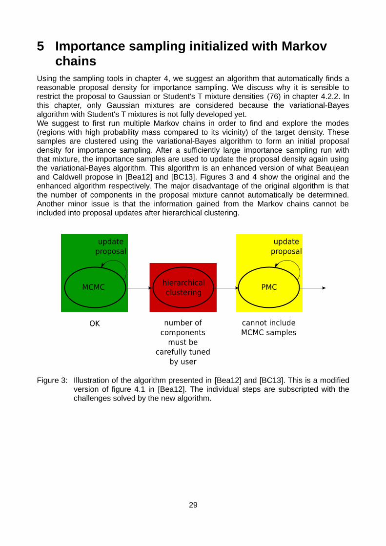
Using the sampling tools in chapter 4, we suggest an algorithm that automatically finds a reasonable proposal density for importance sampling. We discuss why it is sensible to restrict the proposal to Gaussian or Student's T mixture densities (76) in chapter 4.2.2. In this chapter, only Gaussian mixtures are considered because the variational-Bayes algorithm with Student's T mixtures is not fully developed yet.We suggest to first run multiple Markov chains in order to find and explore the modes (regions with high probability mass compared to its vicinity) of the target density. These samples are clustered using the variational-Bayes algorithm to form an initial proposal density for importance sampling. After a sufficiently large importance sampling run with that mixture, the importance samples are used to update the proposal density again using the variational-Bayes algorithm. This algorithm is an enhanced version of what Beaujean and Caldwell propose in [Bea12] and [BC13]. Figures 3 and 4 show the original and the enhanced algorithm respectively. The major disadvantage of the original algorithm is that the number of components in the proposal mixture cannot automatically be determined. Another minor issue is that the information gained from the Markov chains cannot be included into proposal updates after hierarchical clustering.

Figure 3: Illustration of the algorithm presented in [Bea12] and [BC13]. This is a modified version of figure 4.1 in [Bea12]. The individual steps are subscripted with the challenges solved by the new algorithm.

29

Figure 4: Illustration of the enhanced algorithm. This is a modified version of figure 4.1 in [Bea12].

5.1 Markov chain prerun

In this first step, the main goal is to transform the target function P into samples for further processing. Typically, P exists as callable code on a computer but does not have a simple closed-form expression. In particular, we cannot analytically calculate integrals of interest such as expectation values and the evidence. In many cases, only a function proportional to the target distribution P is available. The reason is that every nonnegative integrable function P' : ℝ

d→ℝ0

+ with nonzero integral defines a probability density function

P(x)≡P '( x)/∫P ' (x)d x . We can often formulate P' but, as mentioned before, not analytically integrate it. However, by the strong law of large numbers (cf. chapter 2.3) we can approximate expectation values by a finite number of samples distributed according to P . Hence, we need an algorithm to draw samples from P while we only have its

unnormalized version P' . Looking into chapter 4.1, we find an algorithm that meets this requirement for unimodal target densities. Although local-random-walk Markov chains cannot cope with multimodal target distributions, each chain produces reliable samples of the one mode it is trapped in if run long enough. We therefore run multiple chains and combine the samples as described in chapter 5.2.The resulting Markov chain samples strongly depend on the proposal density and the initial position. How to overcome most difficulties related to the Markov chains is explained in [BC13] and more detailed in [Bea12]. For the toy examples we discuss in this chapter, we run ten chains with a Gaussian proposal density. The initial covariance matrix is set to 0.1 times the unit matrix. Note that this Markov chain step is unchanged compared to the algorithm presented in [BC13]/[Bea12].

5.2 First Proposal for importance sampling

In this step, we want to use the Markov chain samples to generate a Gaussian mixture

q (x∣θ)≡∏n=1

N

q(xn∣θ) , q (xn∣θ)≡∑k=1

K

πk N k (xn∣μ k , Σk) , ∑k=1

K

πk=1, πk≥0 (84)

as proposal density for importance sampling. Given the samples x={x1, ... ,xN} and the number of components K , one approach to minimize the IS related uncertainty is to maximize the likelihood q (x∣θ) with respect to the parameters θ={π ,μ , Σ} (cf. chapter

30

4.2.2). Note that K is implicitly included in θ as μ={μk }k=1K and Σ={Σk}k=1

K . The first question to be addressed is how many components K the mixture should have. A standard approach is to penalize the likelihood for too many free parameters. Then one optimizes a penalized likelihood

~q (θ ,K )≡q(x∣θ)+ penalty (K) , where q (x∣θ)=∏i=1

N

q(xn∣θ) (85)

for several fixed values of K with respect to the parameters θ and chooses the solution that maximizes ~q . A summary of common information criteria (= likelihood penalizations) is given in [BG97]. Note that maximizing the likelihood is an ill-posed problem in the sense that for K≥1 , the likelihood becomes arbitrarily large when a component collapses onto a single sample (see chapter 9.2.1 in [Bis06]). The penalty term is required because surplus components do not change the unpenalized likelihood. Consider for example a maximum likelihood solution for some fixed number of components K . Introducing a new component K +1 with negligible weight πK +1≈0 does not change the unpenalized likelihood.The approach explained above requires to adapt multiple mixtures with different numbers of components. A less compute intensive method is to set a relatively high initial K and remove components whose weights πk drop below some threshold. This can also be motivated by the later use of q (x∣θ) as proposal for IS: Only few samples are drawn from components with small weight. Thus those components do not essentially contribute to the final samples. Moreover, we adapt μ k and Σ k using the samples effectively assigned to component k . If there are too many components, there are not enough samples to accurately learn all the μ k and Σ k .

5.2.1 Hierarchical clustering

Hierarchical clustering is an algorithm that reduces a Gaussian mixture density (84) to another Gaussian mixture with fewer components. The idea is to reduce the complexity while preserving as much information as possible. A full explanation of the algorithm is available in [GR04]. The user has to specify the input mixture and an initial guess for the output mixture. Beaujean and Caldwell [BC13] [Bea12] propose to summarize the Markov chain samples (cf. chapter 5.1) by a Gaussian mixture and then reduce that mixture with hierarchical clustering. In the following, we briefly review their suggestion how to set the input mixture and the initial guess for the output mixture.The input mixture is generated by partitioning the chains into “short patches” of length L , where L is user defined. We use L=100 for the toy examples discussed later in this chapter. Each patch forms a Gaussian component in the initial mixture with sample mean and sample covariance as parameters. All components in the initial mixture are assigned equal weight. The idea behind these short patches is to summarize the small scale features of the target density. The local-random-walk Markov chains slowly diffuse through parameter space such that the short patches summarize local features of the target density. Note that setting all component weights equal does typically not reproduce the correct relative weighting between isolated modes (cf. chapter 4.1). If the target has multiple modes, each local-random-walk Markov chain only explores one of them. The samples of one chain are distributed according to only one of the modes. The probability for a chain to end up in a specific mode is NOT equal to the total probability mass of that mode. Combining multiple chains does therefore NOT reproduce samples that are

31

distributed according to the full target distribution. Nevertheless, the mean values and covariance correctly summarize the local structure of the target.The initial guess for the output mixture is generated from “long patches” in three steps. First, the chains that have explored the same mode are grouped together. Then, the samples of each chain group are split into patches. Finally, Gaussians are created from these patches. Our grouping criterion is the Gelman-Rubin R value proposed in [GR92]. The R value is defined for a group of at least two Markov chains. An R value of O(1) means that the chains have converged (e.g. have explored the same mode). The procedure of grouping the chains is done as follows: The first chain opens a new group. The second chain is inserted into the first group if the R value of both chains is less than a certain user defined critical R value Rcrit (we use Rcrit=2 for the toy examples in this chapter). If the R value is larger than Rcrit , the second chain opens a new group. The next chain is merged into an existing group if the common R value is below the threshold Rcrit , otherwise it opens a new group. This procedure is repeated until all chains are assigned to a group. The initial output mixture is created such that each chain group contributes with Kg components, where the number of components per group Kg is user defined. We use Kg=15 for the toy examples unless stated otherwise. Kg Gaussians are created from a

chain group as follows: If the chain group contains at most K g chains, divide each individual chain in the group into ⌊ Kg /kg ⌋ or ⌈ Kg /kg ⌉ patches6, where k g is the number of chains in the group and the operators ⌈ ⌉ and ⌊ ⌋ denote ceiling and floor. Each patch is summarized as Gaussian component with sample mean and sample covariance. If the chain group contains more chains than K g , combine the individual chains to one long chain. Then k g=1 and the first case applies.

5.2.2 Population Monte Carlo

The PMC algorithm presented in [Kil+09] addresses the problem of improving a Gaussian or Student's T mixture proposal using importance samples. Its input consists of a Gaussian or Student's T mixture and importance-weighted samples. The output is a Gaussian mixture that is “closer” to the target density in the sense of KL(P∥q) (cf. chapter 4.2.2). It is based on the maximum likelihood approach; i.e. it tries to increase q (x∣θ) in each iteration. Like VB, PMC is an EM-like algorithm. In the E-step, PMC calculates the responsibility matrix (similar to what we call r in chapter 3.2) using the fixed input mixture. In the subsequent M-step, the responsibilities are fixed and used to maximize the likelihood q (x∣θ) with respect to the parameters θ . Unlike VB, PMC directly adapts the parameters θ , not a set of hyperparameters.To use PMC, we have to specify its input; i.e. a Gaussian mixture and importance-weighted samples. We use the “long patches” introduced in 5.2.1 as initial Gaussian mixture and the Markov chain samples. Due to the local-random-walk character, the MC samples are highly autocorrelated. We reduce the autocorrelation by taking every 100 th

sample only. All importance weights are set to one, which is not obvious in case of multiple modes. If we assume that all Markov chains are globally converged, then the samples are distributed according to the target distribution. In that case, we can reinterpret the samples as importance samples where proposal and target density are the same. The importance weights are all equal to one then. We know however, that a local-random-walk Markov chain (cf. chapter 4.1) typically only samples from a single mode. Reinterpreted as

6 If kg does not divide K g , it is impossible to make each chain contribute with the same number of components. In that case, the first chains contribute with one more component than the last ones such that the whole group contributes with exactly K g components.

32

importance samples, the proposal function of an individual chain is not the full target density but the target restricted to one mode. Correct sample weighting would require to know the probability mass inside each mode. By setting all weights to one, we assume that all modes have equal integrated probability. The modes are usually well separated such that components in different modes have negligible overlap. As a consequence, the responsibility of a component for a sample in a different mode is insignificant. Thus, PMC tends to locally find accurate Gaussian mixtures but fails to estimate the relative component weights between components located in different modes. The misjudged weights can be corrected in further proposal updates with weighted samples (cf. chapter 5.3).All papers we are aware of ([BC13], [Cap+04], [Cap+08], [Kil+09]) propose to perform only one PMC update with the same set of samples. Multiple updates can lead to “overfitting”. This effect is discussed in more detail in Bishop's book [Bis06], chapter 9.2.1: When a mixture component collapses onto a single sample in one dimension, the likelihood q (x∣θ)

increases with shrinking variance of that one component (N (xn∣μk ,σ k) ∝σ k→ 0

1/σ k∈q (x∣θ)) . In

higher dimensions, the same effect occurs for a singular covariance matrix when a component gets assigned less samples than the dimensionality. Because we prune components with too few effective samples, overfitting is no problem in our approach.We run PMC for exactly 1,000 updates using the output mixture from the previous step as input to the next. Note that PMC offers no intrinsic convergence criterion, see the discussion in chapter 5.2.4 for further details. After each step, we prune components with weight πk less than (2 K)

−1 where K is the number of components of the long patches. The critical component weight (2 K)

−1 is motivated as follows: Suppose the target density is a Gaussian mixture consisting of K t components and all of them have equal weight; i.e. πk=1/ K t ∀ k . It seems sensible to prune components that have much smaller weight than the average. In practice, we have to specify a cutoff that defines “much smaller”. Half of the expected average weight (2 K)

−1 works well on toy targets.

5.2.3 Variational Bayes

A detailed explanation of the variational-Bayes algorithm with Gaussian mixtures can be found in chapter 3.2. Unlike PMC, VB does not directly adapt the parameters of a Gaussian mixture. It rather matches a set of hyperparameters that describe the probability distribution of the parameters. The required input consists of a set of samples, the prior hyperparameters, and an initial guess for the posterior hyperparameters. Like for PMC, we thin the MC samples by a factor of 100. In the following, we explain how to set the prior hyperparameters α0 , m0 , β0 , V0 , and ν0 , and how to initialize their posterior counterparts (without subscript zero).In order to set the hyperparameters we should first try to understand their meaning. The “accuracy parameters” αk (52), βk (54), and νk (56) are all updated as prior value plus effective number of samples N k assigned to component k . They can be interpreted as the number of observations giving rise to our current estimates of the component weights, means, and covariances, respectively. The component mean and covariance estimates themselves are coded into mk and V k . mk denotes mean and mode of the probability distribution for component k 's position μ k . If estimates of the component means or modes are available, they should enter mk . The interpretation of V k is the most difficult. Before interpreting V k , first note that neither the Wishart nor the inverse-Wishart distribution is symmetric. If there is prior knowledge, it is not always obvious whether to tune mean or mode of Σ k 's distribution. Second, note that VB can equivalently be

33

formulated in two ways: Using the inverse-Wishart distribution and covariance matrices or using the Wishart distribution and precision (inverted covariance) matrices. In chapter 3, we present the version with covariance matrices. A formulation in terms of precisions can be found in chapter 10 in Bishop's book [Bis06]. Knowing about both formulations, one has to decide whether to tune either mode or mean of either the covariance Σ k or the precision Σ k

−1 when prior knowledge or a posterior estimate is present. Luckily, the difference between all those approaches becomes negligible for νk≫d because they all result in setting V k=O(νk±d )⋅Σ k . By d , we denote the dimensionality of μk and Σ k .

In our setup, no prior information about the target distribution is available. We therefore tune the hyperparameters to approximate a proper uninformative prior.The accuracy parameters can simply be set to their mathematical lower limits plus some positive number ϵ≪1 . We set α0k=10−5 which means, interpreting the Dirichlet distribution, we know that our prior has too many components. In fact the Dirichlet distribution favors solutions with weight π0 k close to zero if α0 k<1 . The uniform distribution is exactly obtained if all α0k=1 . In practice, it is only important to set all α0k close to one or zero and to have sufficiently many samples N k ≫1 . Note that the Dirichlet distribution constrains α0k>0 , in particular α0 k=0 is forbidden. In the limit β0k→0 the Gaussian in the Normal-Wishart distribution approaches the uniform distribution. We are not allowed to set β0k=0 , so we set β0k=10−5 . ν0 k is constrained by ν0k>d−1 ,

consequently we set ν0k=d−1+10−5 .We do not have prior estimates for the mean values m0 , but we must choose a set of favored points. We can tune m0 such that it has the least impact on m , the posterior component mean estimates. This is achieved for m0=0 because then the update equation for mk (28) is just the mean value of the samples assigned to component k (if we neglect the influence of β0 : βk=β0k+N k≈N k ).In order to set V0 k , best practice is again trying to make its posterior equivalent V k as independent of the prior as possible. Looking at the update equation (29), we see that it should fulfill V0 k≪N k Sk ; i.e. it should be much less than the sample covariance times the number of samples. This cannot be assured in advance, when the sample covariances of the individual components are not known yet. V0 k therefore has to be tuned to the actual problem. We usually set V0 k=I⋅10−10 or V0 k=I⋅10−20 , where I denotes the unit matrix.To summarize, the prior accuracy parameters should be chosen close to their lower bounds, m0=0 , and V0 k should be diagonal and each entry should be much less than the expected posterior component covariances.Our stopping criterion is a relative change of L (q) less than 10−10 or an absolute change of less than 10−5 . In addition, we allow at most 1,000 updates. VB is rather robust against bad initial posterior hyperparameters. We simply use the “long patches” as for hierarchical clustering and PMC. For details refer to the implementation of “GaussianInference” in pypmc (cf. Appendix B). We pass the long patches as “initial_guess”.In order to automatically find a reasonable number of components, we finally have to specify a criterion which components to prune. For VB, we remove a component, when its effective number of samples N k drops below a certain value. By experience, N k <N /2 K long patches prunes only unimportant components provided that enough samples

and initial components are present. This is the same prune criterion as for PMC (πk

PMC<1/2K long patches) since PMC sets the component weights to πk

PMC=N k /N . We check

for removable components after each E-step.

34

The VB output is an approximation of the full probability distribution for the parameters θ={π ,μ , Σ} . We use the mode of the parameter distribution,

πk=αk−1

∑k=1

K

αk−K

if αk>1 else 0, μk=mk , Σ k=( νk−d )−1

⋅V k ,(86)

as parameters for our initial IS proposal. Note that Σ k is determined by the mode of the distribution of its inverse Σ k

−1 . That is because our VB implementation in pypmc (cf. Appendix B) follows the notation of Bishop's book [Bis06] using precision instead of covariance matrices. Other methods to extract parameter values from the distribution are not considered in this work.

5.2.4 Discussion

We compare the algorithms described above mainly by the quality of the importance samples drawn from the resulting proposal (84). Most important is the effective sample size introduced in chapter 4.2.2. With low ESS, more samples and consequently more function evaluations are needed to calculate expectation values, such as the binned marginal likelihood needed for histograms. The perplexity (82) quantifies the distance between target and proposal. We analyze perplexity and effective sample size as a function of the number of Markov chain samples. We would like to keep the Markov chains as short as possible for two reasons. First, Markov chains are purely sequential algorithms, so the ability of massive parallelization as available on a computing cluster cannot speed up the chains. Second, the Markov chain samples are the only samples that do not directly enter the evidence calculation. Another criterion is the ability to reliably determine a reasonable number of components. For this step alone, the number of components is not important. Only in further updates (cf. chapter 5.3), the number of samples needs to grow with the number of components. How many components to take is an open question in the original algorithm [BC13] [Bea12].In our tests, only VB could robustly prune unnecessary components and at the same time achieve at least moderate perplexities and effective sample size. In contrast to hierarchical clustering, VB and PMC optimize the proposal density using the full data set, not just a Gaussian mixture of “short patches”. Consequently these algorithms should be able to produce a better fit in the sense of higher perplexity and ESS (cf. chapter 4.2.2).

5.2.4.1 Asymptotically Gaussian toy target

We first apply the algorithms to an asymptotically Gaussian target:

P(x)=N ( y (x)∣0,Σ )

y (x)={x2−β ( x12−σ1

2 ) i=1

x i i≠1

Σ =diag(σ12 ,1,… ,1)

(87)

35

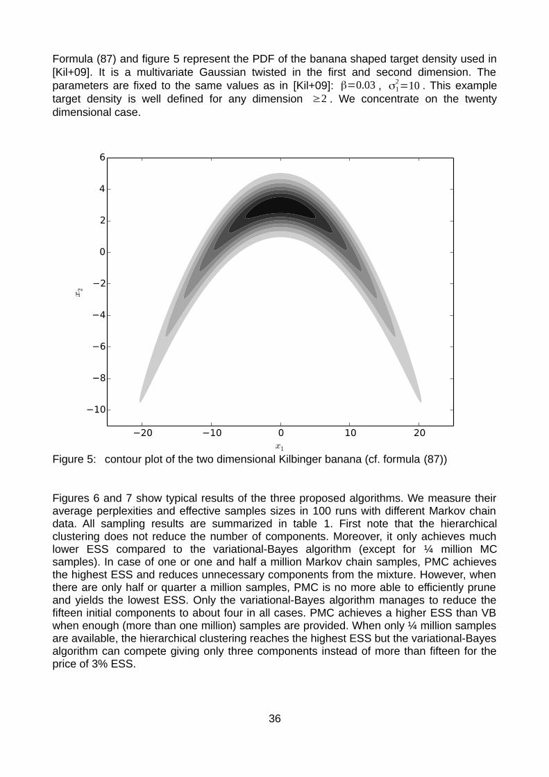
Formula (87) and figure 5 represent the PDF of the banana shaped target density used in [Kil+09]. It is a multivariate Gaussian twisted in the first and second dimension. The parameters are fixed to the same values as in [Kil+09]: β=0.03 , σ1

2=10 . This example target density is well defined for any dimension ≥2 . We concentrate on the twenty dimensional case.

Figure 5: contour plot of the two dimensional Kilbinger banana (cf. formula (87))

Figures 6 and 7 show typical results of the three proposed algorithms. We measure their average perplexities and effective samples sizes in 100 runs with different Markov chain data. All sampling results are summarized in table 1. First note that the hierarchical clustering does not reduce the number of components. Moreover, it only achieves much lower ESS compared to the variational-Bayes algorithm (except for ¼ million MC samples). In case of one or one and half a million Markov chain samples, PMC achieves the highest ESS and reduces unnecessary components from the mixture. However, when there are only half or quarter a million samples, PMC is no more able to efficiently prune and yields the lowest ESS. Only the variational-Bayes algorithm manages to reduce the fifteen initial components to about four in all cases. PMC achieves a higher ESS than VB when enough (more than one million) samples are provided. When only ¼ million samples are available, the hierarchical clustering reaches the highest ESS but the variational-Bayes algorithm can compete giving only three components instead of more than fifteen for the price of 3% ESS.

36

Figure 6: Typical result when running the algorithms discussed in this chapter using 500,000 Markov chain samples (a). The MC data are thinned by a factor 100 and used to infer a Gaussian mixture by hierarchical clustering (b), Population Monte Carlo (c) and the variational-Bayes algorithm (d). The colored ellipses reflect the covariance projected into the first two dimensions.

37

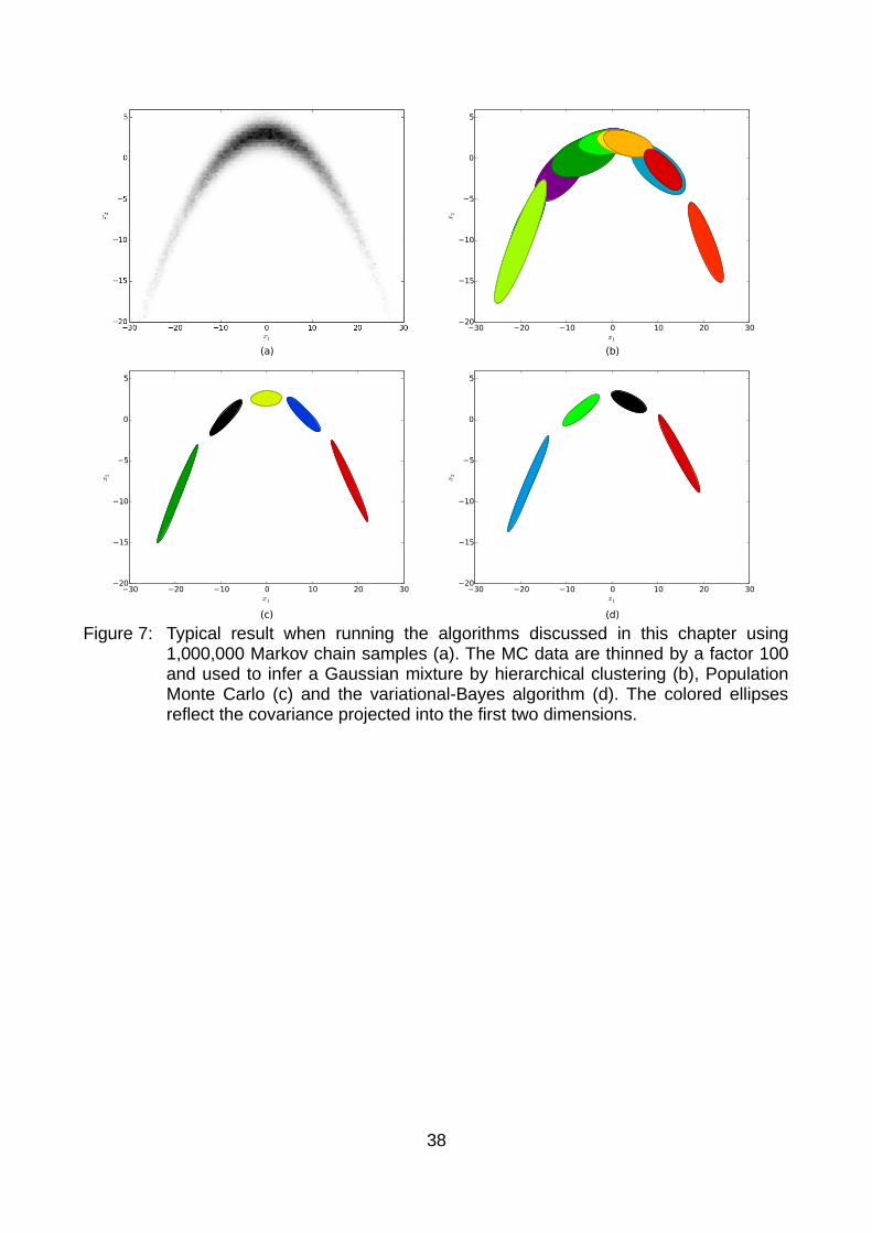
Figure 7: Typical result when running the algorithms discussed in this chapter using 1,000,000 Markov chain samples (a). The MC data are thinned by a factor 100 and used to infer a Gaussian mixture by hierarchical clustering (b), Population Monte Carlo (c) and the variational-Bayes algorithm (d). The colored ellipses reflect the covariance projected into the first two dimensions.

38

HC PMC VB

samples per Markov chain

K final P[%]

ESS[%]

K final P[%]

ESS[%]

K final P[%]

ESS[%]

¼ million16.2±4.1

56.5±8.3

19.5±10.3

12.7±3.7

29.3±9.2

4.69±3.59

3.4±0.6

63.6±8.0

16.7±11.6

½ million15.0±0

61.6±3.4

32.7±12.0

8.6±2.1

68.1±7.9

29.9±13.5

4.0±0.4

77.7±2.9

40.2±15.0

1 million15.0±0

62.2±1.3

41.8±9.0

5.6±1.0

86.8±2.1

63.6±15.1

4.4±0.5

85.1±2.4

60.5±14.6

1½ million15.0±0

61.7±2.6

44.8±8.9

5.3±0.7

89.3±3.5

71.1±15.2

4.7±0.5

87.4±4.0

66.5±16.5

Table 1: Final number of components ( K final ), perplexity ( P ) and Effective Sample Size (ESS) for the banana shaped target (figure 5) averaged over 100 runs. The number of samples stated in the first column is the length of each individual chain before thinning. The errors stated above are calculated as the square root of the sample variance. The notation a±b does NOT imply a Gaussian distribution here.

5.2.4.2 Fat-tailed toy target

We also analyze a target function with nongaussian tails. Student's T mixture proposals are more suitable than Gaussian mixtures in such cases. The tail probability of Student's T distribution can be adjusted by its degrees of freedom parameter. If we want to use Gaussian mixtures anyway, we have to cut the target function down to a compact support. Otherwise, the variance of the integral estimator is infinite. If for example the target density decays polynomially and the proposal density like a Gaussian, then the first integral in (74) does not converge. We only consider Gaussian mixture proposal densities because our variational-Bayes implementation for Student's T mixtures is not ready yet.We benchmark the different algorithms on the multimodal toy target density

P(x)={sin( x1

2 )10

(1+sin( x2

2 )2

)∏i=3

d

min ( 14,

1

xi2 ) ∀ x i : −6<x i<6

0 else

. (88)

In this section. The density denoted in (88) is plotted in figure 8. The multimodal target is defined in all dimensions d≥2 but we only consider the twenty dimensional case.

39

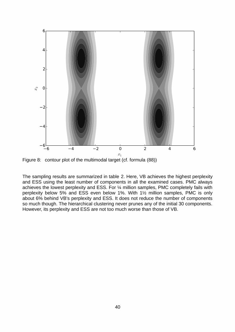
Figure 8: contour plot of the multimodal target (cf. formula (88))

The sampling results are summarized in table 2. Here, VB achieves the highest perplexity and ESS using the least number of components in all the examined cases. PMC always achieves the lowest perplexity and ESS. For ¼ million samples, PMC completely fails with perplexity below 5% and ESS even below 1%. With 1½ million samples, PMC is only about 6% behind VB's perplexity and ESS. It does not reduce the number of components so much though. The hierarchical clustering never prunes any of the initial 30 components. However, its perplexity and ESS are not too much worse than those of VB.

40

Figure 9: Typical result when running the algorithms discussed in this chapter using 1,500,000 Markov chain samples (a). The two modes have equal probability mass. The right mode looks more important because it is mapped out by more chains. The MC data are thinned by a factor 100 and used to infer a Gaussian mixture by hierarchical clustering (b), Population Monte Carlo (c) and the variational-Bayes algorithm (d). The colored ellipses reflect the covariance projected into the first two dimensions.

41

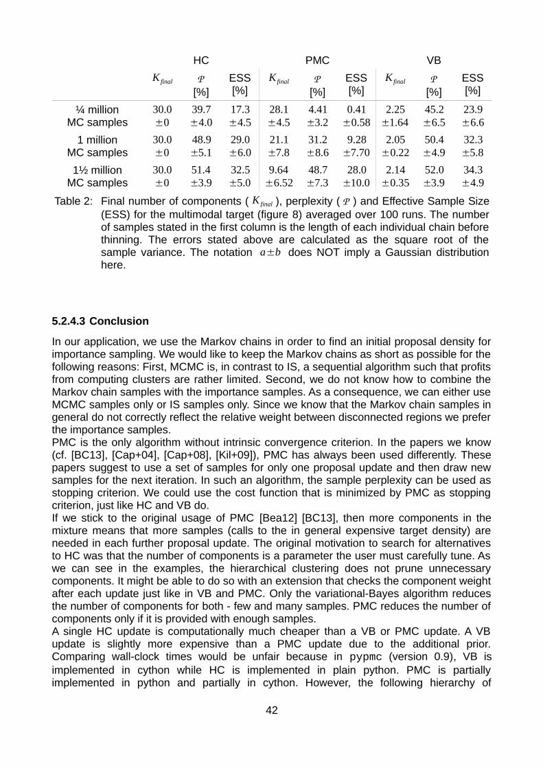
HC PMC VB

K final P[%]

ESS[%]

K final P[%]

ESS[%]

K final P[%]

ESS[%]

¼ millionMC samples

30.0±0

39.7±4.0

17.3±4.5

28.1±4.5

4.41±3.2

0.41±0.58

2.25±1.64

45.2±6.5

23.9±6.6

1 millionMC samples

30.0±0

48.9±5.1

29.0±6.0

21.1±7.8

31.2±8.6

9.28±7.70

2.05±0.22

50.4±4.9

32.3±5.8

1½ millionMC samples

30.0±0

51.4±3.9

32.5±5.0

9.64±6.52

48.7±7.3

28.0±10.0

2.14±0.35

52.0±3.9

34.3±4.9

Table 2: Final number of components ( K final ), perplexity ( P ) and Effective Sample Size (ESS) for the multimodal target (figure 8) averaged over 100 runs. The number of samples stated in the first column is the length of each individual chain before thinning. The errors stated above are calculated as the square root of the sample variance. The notation a±b does NOT imply a Gaussian distribution here.

5.2.4.3 Conclusion

In our application, we use the Markov chains in order to find an initial proposal density for importance sampling. We would like to keep the Markov chains as short as possible for the following reasons: First, MCMC is, in contrast to IS, a sequential algorithm such that profits from computing clusters are rather limited. Second, we do not know how to combine the Markov chain samples with the importance samples. As a consequence, we can either use MCMC samples only or IS samples only. Since we know that the Markov chain samples in general do not correctly reflect the relative weight between disconnected regions we prefer the importance samples.PMC is the only algorithm without intrinsic convergence criterion. In the papers we know (cf. [BC13], [Cap+04], [Cap+08], [Kil+09]), PMC has always been used differently. These papers suggest to use a set of samples for only one proposal update and then draw new samples for the next iteration. In such an algorithm, the sample perplexity can be used as stopping criterion. We could use the cost function that is minimized by PMC as stopping criterion, just like HC and VB do.If we stick to the original usage of PMC [Bea12] [BC13], then more components in the mixture means that more samples (calls to the in general expensive target density) are needed in each further proposal update. The original motivation to search for alternatives to HC was that the number of components is a parameter the user must carefully tune. As we can see in the examples, the hierarchical clustering does not prune unnecessary components. It might be able to do so with an extension that checks the component weight after each update just like in VB and PMC. Only the variational-Bayes algorithm reduces the number of components for both - few and many samples. PMC reduces the number of components only if it is provided with enough samples.A single HC update is computationally much cheaper than a VB or PMC update. A VB update is slightly more expensive than a PMC update due to the additional prior. Comparing wall-clock times would be unfair because in pypmc (version 0.9), VB is implemented in cython while HC is implemented in plain python. PMC is partially implemented in python and partially in cython. However, the following hierarchy of

42

computational effort should hold if all three algorithms were implemented in the same programming language: HC is much less expensive than PMC is slightly less expensive than VB.The algorithm to be considered “best” depends on the target distribution and the available computing resources. The important quantities we want to calculate are expectation values like (72). We can reduce the uncertainty of the importance sampling estimates in two ways, an improved proposal (see chapter 4.2.2) and more samples (see equation (74)). In total, we want as accurate estimates as possible in a minimal amount of time. If the target density is easy to evaluate, then a less expensive but less accurate proposal adaptation (eg HC) and more importance samples (more target evaluations) may be faster than running PMC or VB at all.

5.3 Further proposal updates

When we have a proposal density from the Markov chains, we could in principle just use it for importance sampling without any further adaptation. However, further improvements in perplexity and effective sample size can be reached with additional data. When the target has multiple modes (like in the multimodal example), the component weights cannot be learned from the Markov chains. In which mode a chain ends up, rather depends on the size of the mode's support and the chain's initial position than on the mode's total probability (cf chapter 4.1). Importance samples however contain the globally correct weighting information.One should never use PMC to cluster the Markov chains and then VB for subsequent proposal updates or vice versa. According to our experience, perplexity and effective sample size decrease when PMC and VB are mixed. The reason is that PMC and VB converge into different solutions. Consequently, it doesn't make sense to consider further adaptations regardless of the algorithm that produced the initial proposal. We compare the complete original algorithm (cf. figure 3) to our proposed enhancement (cf. figure 4). Both algorithms are reviewed in the following.

5.3.1 Original algorithm

In the original algorithm, the first proposal is generated by hierarchical clustering as described in chapter 5.2.1. The resulting mixture is then used as proposal for importance sampling. In total N IS=K⋅N c importance samples are drawn from the first proposal, where the user has to define the number of samples per component N c . In the examples provided in this chapter we choose N c=600 . The importance samples and the mixture density are then passed to PMC. After a single PMC update, the PMC output mixture is used to draw K⋅Nc importance samples. These samples and the newly obtained mixture are passed back to PMC for an update. PMC and importance sampling are iterated for at most 25 times until the sample perplexity increases less than 5%,

( P t−P t−1)P t−1

< 5% , (89)

where t enumerates the proposal update steps. A component that gets less than twenty samples assigned in a PMC step is removed.An exhaustive explanation is provided in [Bea12], a detailed summary can be found in [BC13].

43

5.3.2 Enhanced algorithm

In the new algorithm, we basically replace the hierarchical clustering and PMC by the variational-Bayes algorithm. The first proposal is generated as described in chapter 5.2.3, the further updates are discussed below. The alternatives to HC described in chapter 5.2 already yield a quite good proposal. As a consequence, further updates are degraded to optional improvements on not-too-hard problems.The variational-Bayes algorithm (cf. chapter 3.2) updates the probability distribution of the parameters θ={π ,μ , Σ} of a Gaussian mixture. The prior distribution of the parameters is parametrized by a set of hyperparameters Θ0

t ={α0t ,m0

t ,β0t ,V0

t , ν0t } where t indexes the

number of proposal updates; t=0 indicates the VB run with MCMC data. The variational posterior takes the same functional form but with updated hyperparameters Θ

t={α

t ,mt ,βt ,V t ,ν t} . For subsequent proposal updates, we could forward the parameter

distribution obtained in the previous step as informative prior; i.e. we could set

Θ0t +1=Θt . (90)

We do NOT follow this procedure because the variational posterior is an APPROXIMATION of the true posterior. Consequently, equation (90) introduces an approximation every time it is applied. We therefore recommend to rather use the sample combination described in chapter 5.4 and plug the importance samples into VB altogether. The procedure we follow is sketched in figure 10. We always combine all available importance samples and impose the informative prior obtained from MCMC with the following exception:Special care has to be taken of α

t=0 , the hyperparameter that describes the component weights inferred from the Markov chain data. If the target has multiple disconnected regions, the Markov chains do not reproduce the correct component weights (cf. chapter 4.1). Consequently, the probability distribution of the component weights inferred with the Markov chain data is incorrect. We account for this additional knowledge by setting α0 k

t≥1=10−5≠αkt =0 ; i.e. we impose the same uninformative prior for the component weights

as in the first VB run (cf. chapter 5.2.3).

Our choice of Θ0t≥1

={α0t≥1,m0

t≥1 ,β0t≥1 ,V 0

t≥1 ,ν 0t≥1

} codes exactly the information we gain from the Markov chains: We have valid estimates for the component means μ and covariances Σ that are coded by m0

t≥1 and V0t≥1 . Both of them rely on a finite number of samples that

are coded into β0t ≥1 and ν0

t≥1 . We know the guess of the component weights π could be wrong. We therefore set α0

t≥1 such that it approximates “not watched yet”.The estimate of π is incorrect only if the Markov chains have not explored the full parameter space. Whenever the target distribution is unimodal and the chains are run long enough, the component-weight estimates coded by α

t =0 are reliable. If we can assure that all chains have mixed, for example because they are all assigned to the same group by the Gelman-Rubin R value (cf. chapter 5.2.1), the results would probably improve if we set α0

t ≥1=α

t=0 . However, we stick to the setting α0kt≥1

=10−5≠αk

t=0 in any case throughout this thesis.In contrast to PMC in the original algorithm, VB has access to the information extracted from the Markov chains by the informative prior. Nevertheless, our prior lacks informative component-weight estimates α0

t . Like in the original algorithm, the component weights are

44

exclusively derived from importance sampling. In the following, we discuss how to set the number of importance samples N IS

t to be drawn from each proposal. The only really critical behavior of the variational-Bayes algorithm is that important components may be removed if N IS

t is too small. But that actually is a consequence of a desired feature: We want components that get few effective samples assigned to be removed. One should therefore choose N IS

t =1≫K to ensure that every component has a chance to survive.

During later proposal updates, we include all earlier samples such that N ISt

≫K for t>1 is

automatically fulfilled if N ISt =1≫K . As a side remark note that the number of samples is

totally uncritical if the variational-Bayes algorithm is run with a full informative prior.

For the toy examples discussed in the next section, we run VB only once with N IS=6,000 importance samples. This is motivated by the fact that we already have a pretty good proposal from the MCMC data. In fact, most often the old convergence criterion (89) would indicate convergence after the first VB run with importance samples. Like in the first VB run, we stop when the log-likelihood bound L (q) changes less than 10−10 relative or less than 10−5 absolute or after a thousand steps. Components with less than one effective sample are pruned.

Figure 10: Sketch of the enhanced algorithm. The samples from multiple Markov chains are clustered by the variational-Bayes algorithm. The resulting proposal is used for Importance sampling. Optional further proposal updates use the variational posterior of the very first VB run as prior and all available importance samples as data. Authored by Frederik Beaujean; taken with the author's permission.

45

5.3.3 Discussion

The original algorithm uses PMC exactly like it is suggested in the literature ([Cap+04], [Cap+08], [Kil+09]). In particular, each PMC update is performed with new samples. The original algorithm therefore needs more target evaluations than the enhanced version. However, generating the first proposal using VB is more expensive than HC. While the hierarchical clustering converges after O(10) steps, the first variational-Bayes run typically needs O(500) steps. In addition, a VB step is more expensive than a HC step. For the price of lower perplexity and ESS and more components, the number of VB steps can be reduced by imposing looser convergence criteria (e.g. less than a relative change of 10−5 or an absolute change of 10−3 in the log-likelihood bound). But even then, VB still needs O(100) steps to converge.If the first proposal is not too bad, further updates using VB converge in O(10) steps. According to our experience, if the variational-Bayes algorithm needs much more than ten steps in further updates, then the Markov chains did not explore all of their modes. The computational effort concerning only further proposal updates (not considering calls to the target) is comparable to the old algorithm. PMC and importance sampling must be iterated O(10) times until convergence; i.e. O(10) PMC update steps must be run. Nevertheless, the old algorithms needs much more samples and thus target evaluations.For an easy to evaluate target density, many evaluations are not a problem. However, a single call to the target density we map out in chapter 6 takes a few seconds. Thus, our problem requires an algorithm with as few function evaluations as possible. Note that more samples (and consequently more target evaluations) is always a possibility to increase the effective number of samples N eff ≡ESS⋅N even with a bad (low ESS) proposal. If the target is much faster to evaluate than the proposal updates, it can be better to draw more importance samples from a less well adapted proposal.To summarize, hierarchical clustering to obtain the first proposal is in general faster but worse than the variational-Bayes algorithm (cf. chapter 5.2). Further updates have comparable computational effort concerning VB and PMC but the old algorithm needs much more target evaluations. ESS and perplexity of the old algorithm are lower than those of the enhanced algorithm (cf. table 3). It depends on the time a target evaluation takes whether the old or the new algorithm is faster to produce the desired effective number of samples N eff ≡ESS⋅N .

Note that the time spent with importance sampling can be tuned against the time spent with proposal updates by minor modifications in both algorithms. We can run multiple PMC updates using the same set of importance samples, similar to what we suggest in chapter 5.2.2. That reduces the number of target evaluations while it increases the number of PMC updates. We can soften the convergence criteria for the variational-Bayes algorithm. Then we get a proposal that produces samples with lower ESS and we need more importance samples to obtain the same number of effective samples. Cornuet et al. [Cor+12] propose a combination of importance samples from multiple proposal densities. Their combination allows to always run PMC using all available samples. That increases the time needed for a single PMC update but probably decreases the number of PMC steps needed until convergence. It also allows to include all samples into the evidence calculation and histogram plots; i.e. it shortens the final run (cf. chapter 5.4). We review their method in chapter 5.4.

46

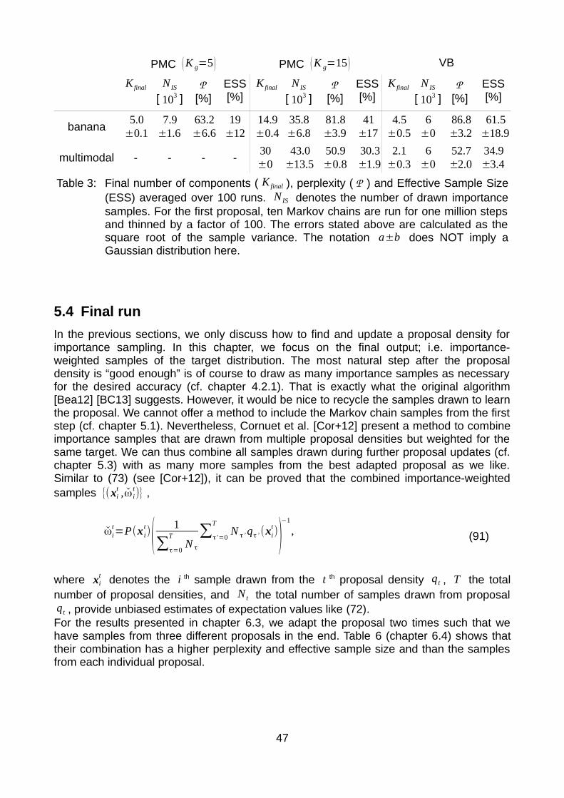
PMC ( K g=5 ) PMC ( K g=15 ) VB

K final N IS

[ 103 ]P

[%]ESS[%]

K final N IS

[ 103 ]P

[%]ESS[%]

K final N IS

[ 103 ]P

[%]ESS[%]

banana5.0

±0.17.9

±1.663.2±6.6

19±12

14.9±0.4

35.8±6.8

81.8±3.9

41±17

4.5±0.5

6±0

86.8±3.2

61.5±18.9

multimodal - - - -30±0

43.0±13.5

50.9±0.8

30.3±1.9

2.1±0.3

6±0

52.7±2.0

34.9±3.4

Table 3: Final number of components ( K final ), perplexity ( P ) and Effective Sample Size (ESS) averaged over 100 runs. N IS denotes the number of drawn importance samples. For the first proposal, ten Markov chains are run for one million steps and thinned by a factor of 100. The errors stated above are calculated as the square root of the sample variance. The notation a±b does NOT imply a Gaussian distribution here.

5.4 Final run

In the previous sections, we only discuss how to find and update a proposal density for importance sampling. In this chapter, we focus on the final output; i.e. importance-weighted samples of the target distribution. The most natural step after the proposal density is “good enough” is of course to draw as many importance samples as necessary for the desired accuracy (cf. chapter 4.2.1). That is exactly what the original algorithm [Bea12] [BC13] suggests. However, it would be nice to recycle the samples drawn to learn the proposal. We cannot offer a method to include the Markov chain samples from the first step (cf. chapter 5.1). Nevertheless, Cornuet et al. [Cor+12] present a method to combine importance samples that are drawn from multiple proposal densities but weighted for the same target. We can thus combine all samples drawn during further proposal updates (cf. chapter 5.3) with as many more samples from the best adapted proposal as we like. Similar to (73) (see [Cor+12]), it can be proved that the combined importance-weighted samples {(xi

t ,ω it)} ,

ωit=P(x i

t)(

1

∑τ=0

TN τ

∑τ '=0

TN τ ' qτ ' (xi

t))

−1

, (91)

where xit denotes the i th sample drawn from the t th proposal density q t , T the total

number of proposal densities, and N t the total number of samples drawn from proposal q t , provide unbiased estimates of expectation values like (72).For the results presented in chapter 6.3, we adapt the proposal two times such that we have samples from three different proposals in the end. Table 6 (chapter 6.4) shows that their combination has a higher perplexity and effective sample size and than the samples from each individual proposal.

47

6 Bayesian analysis of new physics in rare B decays

In this chapter, we analyze if there is evidence for physics beyond the standard model (SM) in rare B-meson decays analogous to [BBD14]. Furthermore, we improve the constraints on scalar, pseudoscalar and tensor Wilson coefficients. The outline of this chapter is as follows: We first describe the theory in chapter 6.1. Our analysis method is described in chapter 6.2. We state and discuss the posterior distribution of the Wilson coefficients and the Bayes factor between the models EFT and SM (see chapter 6.2) as results in chapter 6.3. Finally, we evaluate the performance of our new algorithm in chapter 6.4.

6.1 Theory of rare B decays

Effective field theories (EFTs) allow the theoretical treatment of high-energy physics without knowing its exact structure. The EFT concept in a nutshell can be seen in figure 11: By integrating the heavy W- and Z-bosons out of the standard model, effective operators with effective couplings like C 9 and C 10 arise. The effective couplings capture all heavy particles that can run in the loop, including particles beyond the standard model if present. All heavy fields ( W± , Z0 , top quark, heavy beyond SM) are summarized in the Wilson coefficients whereas the low-energy fields (bottom and lighter quarks, photon, gluon) remain active in the effective theory. A detailed introduction to the concept of EFT is provided in [Neu05] and [Bur98].

Figure 11: Example of leading-order contributions to b→ s ℓ ℓ transitions in (a) the standard model and (b) the effective field theory defined by (92)

We analyze transitions of a b-quark to an s-quark and a lepton-antilepton pair ℓ ℓ in a low-energy effective theory. The b→ s ℓ ℓ effective Hamiltonian reads (cf. [Dyk12], [CMM97], [BHP07])

48

Z0

(a)

W±

,

ℓ ℓ

b s

¯

u ,c , tu , c , tC9,10

ℓ ℓb s

(b)

¯

Heff =−4GF

√2V tbV ts

*(C 1O1c+C2O2c+ ∑

i≠1⋅,2⋅

CiOi)

−4GF

√2V ubV us

*(C1(O1c−O1u)+C 2(O2c−O2u))

+ ... + h.c.

(92)

with the operator basis

O1 c=[ s μT a PL c] [ c μT a PLb ] , O1 u=[ s μT a PLu ][ u μ T a PLb] ,

(93)

O2 c=[ s μ PLc ][ c μ PLb] , O2 u=[ s μ PLu] [u μ PLb ] ,

O3=[ s μ PLb ]∑q[q μ q ] , O5=[ s μ ν ρ PLb]∑q

[ q μ ν ρ q] ,

O4=[ s μT a PLb ]∑q[ q μ T aq ] , O6=[ s μ ν ρT a PLb ]∑q

[ q μ ν ρT a q] ,

O7=e

(4 π )2mb [ s σ

μ νPR b] Fμ ν , O9=

e2

(4 π )2[ s μ PL b][ ℓ μℓ] ,

O8=gs

(4 π )2mb [ s σ

μ ν T a PR b]Gμ νa , O10=

e2

(4 π )2[ s μ PLb ][ ℓ μ 5 ℓ] ,

OS=e2

(4 π )2[ s PR b ][ ℓ ℓ ] , OP=

e2

(4 π )2[ s PR b ][ ℓ 5ℓ] ,

(94)

OT=e2

(4 π )2[ s σμ ν b ][ ℓσμ νℓ] , OT 5=

e2

( 4π )2[ s σμ ν b] [ ℓσμ ν 5ℓ] ,

the Fermi constant GF , and the CKM matrix elements V ij , i∈{u , c ,t }, j∈{d , s , b} . We also consider the chirality-flipped operators O7

' , O9' , O10

' , OS' , and OP

' where the left projector PL=(1−5)/2 is replaced by the right projector PR=(1+ 5)/2 and vice versa. We neglect electroweak penguin operators; i.e. operators including sums like

∑qeq [q Γq ] , (95)

where Γ denotes a combination of Dirac matrices and eq the quark charge.

This work is focused on constraining the scalar (C S , CS') , pseudoscalar (CP , CP

') , tensorial

(CT) , and pseudotensorial (C T 5) Wilson coefficients. Their corresponding operators (94) do not arise in an effective low-energy theory based on integrating heavy fields out of the standard model [BHP07]. Consequently, nonzero values can only be generated by new physics.Quarks can only be indirectly observed as hadrons. In experiments, we can only generate hadronic initial states and observe hadronic final states. We therefore have to consider

49

experimentally tractable decays of hadrons with b-quark content. The simplest possible hadrons consist of a quark and an antiquark - the mesons. Instead of b→ s ℓ ℓ transitions at the quark level, we consider decays of mesons with bottom-quark content (B-mesons). To be precise, we consider CP-averaged observables of the decays B s→ℓ+ ℓ− , B±

→K±ℓ+ ℓ− , and B0→K *0ℓ+ ℓ− . Our nomenclature of B- and K-mesons follows [PDG14].

Detailed theoretical calculations are not within the scope of this work, we just summarize the most important facts here. The calculation of hadronic decay amplitudes is a highly nontrivial task due to nonperturbative QCD. The decays B →K (*)ℓ+ℓ− require a different theoretical treatment in the high and the low q2 regime where different approximations are valid. By q2 , we denote the dilepton invariant mass. High q2 is associated with low hadronic recoil (momentum of the final K (*)

) and low q2 is associated with large hadronic recoil. For high q2 (q2

≥14GeV 2) , an operator product expansion [GP04] is used to

calculate higher orders in perturbation theory. At low q2 (1GeV 2≤q2

≤6GeV 2) , we use

QCD factorization (QCDF) as described in [BFS01]. At leading order both procedures coincide with the so-called naïve factorization,

⟨K (*) ℓ ℓ|[ s Γ1b ][ ℓ Γ2 ℓ]|B⟩=⟨ K (*)|[ s Γ1 b]|B ⟩⟨ ℓ ℓ|[ ℓ Γ2ℓ ]|0⟩ , (96)

where Γ1,2 denote combinations of Dirac matrices as they appear in the operators (93) (94). We disregard the intermediate region 6GeV 2

<q2<14GeV 2 because it is plagued by

large nonperturbative contributions from hadronic resonances (J/ and ') [Wei+09]. The hadronic matrix elements ⟨K (*)|[ s Γ1 b]|B⟩ define the B →K form factors f 0,+, T [BHP07] and the B→K * form factors V , A0,1,2,3 , T1,2,3 [BZ05]. At large recoil, the form factors can be calculated from light-cone sum rules [BB98]. At low recoil, lattice calculations are available [HPQCD13] (see also Appendix C.1).Loop corrections are calculated in the MS

________

renormalization scheme at the scale μ=4.2GeV ≈mb , where mb denotes the MS

________

b-quark mass. The calculation of observables is performed using the EOS flavor program [EOS]. For sampling the posterior, we use the pypmc (cf. Appendix B) implementation of the algorithm described in chapter 5. Since the considered experimental input consists of CP-averaged observables only, we assume no CP violation beyond the SM; i.e. real Wilson coefficients.The theory provides a mapping from parameters (here the Wilson coefficients C i

(,) ) to observables. In the following, we reference the theoretical calculations of the observables used in the next section. Furthermore, we motivate our choice of observables from the theoretical point of view. The overall goal is to infer (constrain) the Wilson coefficients C 10

(,) , C S(,) ,C P

(,), C T , and C T 5 from experimental data while keeping the other Wilson coefficients fixed at their standard model values. Roughly speaking, we want to invert the mapping provided by theory. We show how to do that using Bayes' formula in chapter 6.2.

EOS implements the B s→ℓ+ ℓ− branching ratio as calculated in [Bob+01]. There are no (pseudo)tensor contributions to B s→ℓ+ ℓ− decay amplitudes but the (pseudo)scalar contributions are enhanced compared to SM contributions. Because of the vanishing vector-current matrix element,

⟨0|s μb|B s⟩=0 , (97)

50

every Wilson coefficient can only appear together with its chirality-flipped counterpart as C i−C i

,.The B±

→K±ℓ+ ℓ− normalized angular differential decay width (cf. equation (1.2) in [BHP07]),

1Γ

d Γ

dcos θ=

34

( 1−FH ) (1−cos2θ )+

12

FH +A FBcos θ , (98)

and the (binwise) integrated branching fraction

B=1

Γtot∫ dq2 dΓ

dq2 (99)

are calculated in [BHP07] for large and in [BHD13] for low recoil of the K meson. The operators specified in (94) enter the B±

→K±ℓ+ ℓ− branching ratio B at the same order as the SM contributions. In the forward-backward asymmetry A FB and the flat term FH , (pseudo)scalar and tensor contributions are even enhanced by a factor of √q2

/mℓ (remember that we only consider q2

≥1GeV 2 and that mℓ=μ≈0.1GeV ). In contrast to B s→ℓ+ ℓ− decays, the pseudovector-current related matrix elements of B±

→K±ℓ+ ℓ− amplitudes vanish,

⟨K -|s μ 5 b|B- ⟩=0 , (100)

and therefore the Wilson coefficients can only appear as C i+C i, . In order to constrain all

Wilson coefficients simultaneously, we require additional observables to resolve degeneracies. We therefore also include the B0

→K *0ℓ+ ℓ− branching ratio into our analysis. The decay width of B0

→K *0ℓ+ ℓ− is described in [BHD13] for low and in [BHP08] for large K* recoil.

6.2 Methodology

Our primary goal is to map out the probability distribution of the Wilson coefficients C given experimental data D using Bayes' theorem (cf. chapter 2.2). Furthermore, we want to judge whether the data are in favor of new physics. We therefore compare two models, the model where we infer the Wilson coefficients from the data, and the model where we fix the Wilson coefficients to their standard model values (cf. Appendix C.2). We denote these by EFT and SM .Being theorists, we are not interested in modeling a detector but rather want to rely on experimentalists' publications. The idea is that the experimentalists reduce their full data set consisting of events in their detectors to the likelihood P(D∣O) , where O is a set of relevant “observables”. P(D∣O) as a function of O is taken from experimentalists' publications. Although Bayesian analyses are uncommon in experimental physics, we assume that their publications provide distributions that approximate

P(D∣O)=∫ d νex P(D∣O , νex )P(ν ex∣O) ; (101)

51

i.e. the distribution where experimental nuisance parameters νex are properly marginalized out. We further assume that the likelihood P(D∣O) and the experimental nuisance parameters νex are independent7 of the model M and the theory parameters θ . The theory defined in chapter 6.1 provides a model-dependent mapping from theory parameters θ={C , νth} to observables O such that the likelihood of θ in the model M can be formulated as

P(D∣θ ,M)=P (D∣O (θ ,M)) . (102)

Take for example the angular distribution of the decay B →K ℓ+ ℓ− denoted in (98). The measurable distribution is completely defined by the observables O={AFB ,F H} that themselves can be calculated from the theory as A FB= AFB(θ ,M) and FH=FH (θ , M) . We can split the calculation of P(D∣θ ,M) into two parts, the probability of the data given the relevant observables P(D∣O) and the observable prediction from theory O(θ ,M ) for a given model M and its theory parameters θ . Given these, we can formulate

P(C ,νth∣D ,EFT) ∝Bayes

P (D∣C , νth ,EFT ) P0(C , νth∣EFT)

= P(D∣O(C , νth ,EFT)) P0(C ,νth∣EFT )(103)

and

P(νth∣D ,SM) ∝Bayes

P (D∣νth ,SM) P0(νth∣SM)

= P(D∣O(νth ,SM))P0(ν th∣SM)(104)

using Bayes' theorem (4) and (102).We split the theory parameters into the Wilson coefficients we want to infer from the data8 C ={C 10

(,) ,C S(, ), C P

(,) , C T , C T 5} and other parameters νth (such as quark masses or the CKM matrix elements). A complete description of the so-called nuisance parameters νth can be found in chapter 6.2.2.Formula (103) is the key equation of our method. It describes how to calculate the posterior P(C ,νth∣D ,EFT) (which is what we want to know) from the likelihood P(D∣O) as a function of observables O , the mapping from parameters to observables O(C ,ν th , EFT), and the parameter prior P0(C ,νth∣EFT) . Note that we assume the likelihood P(D∣O) to depend on the underlying model M∈{EFT ,SM , ...} only via the set of relevant observables O . For the example of the B →K ℓ+ ℓ− angular distribution that means we only consider theories that predict an angular distribution as denoted in (98) but the observables O={AFB ,F H} may differ between the different models.The main tool to cope with the posterior P(C ,νth∣D , EFT) are importance-weighted samples (cf. chapter 4.2) drawn using the algorithm described in chapter 5. The model

7 Note that this is an assumption we have to make but it is not always entirely true. The current B →K *ℓ+ ℓ− angular analysis by LHCb for example assumes that there are no (pseudo)scalar and tensor

operators (cf. section 6.2.1); i.e. it does depend on the model M .8 In principle, we would like to infer all Wilson coefficients but for practical reasons, we have to restrict our

analysis. For example, we assume all Wilson coefficients to be real because we only consider measurements of CP-averaged observables.

52

EFT allows deviations of the Wilson coefficients from the standard model predictions. To judge whether the data are in favor of new physics, we use the importance samples to calculate the evidence

ZM=∫ dθ P (D∣O(θ ,M)) P0(θ∣M) , M∈{EFT ,SM}, θ={C , νth if M=EFT

νth if M=SM(105)

and the Bayes factor (cf. chapter 2.2) between the models EFT (103) and SM (104). Furthermore, we can use the samples to draw marginal distributions of the posterior. The results are presented in chapter 6.3.A description of included measurements is listed in chapter 6.2.1. We specify the parameters and their priors in chapter 6.2.2. For the theory calculation O(θ ,M ) (cf. chapter 6.1), we use the EOS flavor program [EOS].

6.2.1 Experimental constraints

We consider the latest experimental results from LHCb, CDF, and CMS. Our main interest is in the new 2014 LHCb results of the angular B±

→K±μ

+μ

− observables (cf. formula (98)) published in [LHC14B]. The recent measurement provides an angular analysis to so far unrivaled accuracy. As mentioned in the previous chapter, the B±

→K±μ

+μ

− angular observables are very sensitive to (pseudo)scalar and (pseudo)tensor operators. We include the integrated branching fractions, A FB , and FH (all CP-averaged) in the bins q2

∈[ 1.10,6.00 ] GeV 2 and q2∈[ 15.00,22.00 ] GeV 2 as stated in [LHC14A] and [LHC14B] into

our likelihood. We further include the (CP-averaged) measurements of A FB and the integrated branching fraction in the bins q2

∈[ 1.00,6.00 ] GeV 2 , q2∈[ 14.18,16.00 ] GeV 2 , and

q2∈[ 16.00,22.86 ] GeV 2 from [CDF12].We also impose the combined CMS-LHCb [Arc14] measurement of the total branching fraction for the (CP-averaged) decay B s→μ

+μ

− .Unfortunately, the angular analysis of B0

→K * 0μ

+μ

− decays carried out by LHCb [Cia14] assumes no contributions from the operators (94) that we are interested in. The main reason for this is that they claim to have too few events to fix all parameters in their fit. We can therefore only consistently include the integrated branching ratio of B0

→K *0μ

+μ

− decays. To be precise, we consider the measurements of the integrated and CP-averaged B0

→K *0μ

+μ

− ( B0→ K* 0μ+μ−) branching ratio in the bins q2∈[ 1.00, 6.00 ] GeV 2 , q2

∈[ 14.18,16.00 ] GeV 2 , and q2∈[ 16.00,19.00 ] GeV 2 published in [LHC13B], [CMS13], and

[CDF12]. Note that the last q2 -bin in [CDF12] is slightly wider q2∈[ 16.00,19.21 ] GeV 2 .Note that there are indications of lepton-flavor-universality violation [LHC14C]. We therefore do not include BaBar [BaBar12A] [Babar12B] and Belle [Belle09] data because they average over the two lepton flavors ℓ=μ and ℓ=e . Instead, we only include purely muonic (ℓ=μ) decays; i.e. we fit the muonic Wilson coefficients. Further note that all included measurements provide only CP-averaged observables. Since we do not include observables sensitive to CP violation, we consider only real Wilson coefficients; i.e. we assume no CP violation beyond the Standard model.

53

6.2.2 Parameters and priors

We denote the theory parameters θ={C , νth} as combination of the Wilson coefficients C ={C 10

(,) ,C S(, ), C P

(,) , C T , C T 5} and the nuisance parameters νth . Our nuisance parameters νth are: The CKM matrix in modified Wolfenstein parametrization, the charm and the

bottom quark mass, the B →K and B→K * form factors in the parametrization presented in [KMPW10], the B s decay constant f Bs

, and subleading corrections. Other “parameters” (eg. the Wilson coefficients C 1−9

(,) ) that can affect the relevant observables (cf. chapter 6.2.1) are considered as part of the model M (cf. chapter 6.2) and kept fixed while we sample through the parameters θ . The reason to include nuisance parameters at all is uncertainty propagation. In order to account for theory uncertainties, we include them as nuisance parameters with an informative prior. The posterior distribution of the Wilson coefficients (where the nuisance parameters are marginalized out) then contains the correctly propagated uncertainty of the nuisance parameters.

We impose a factorizable prior,

P0({C ,ν th})=∏i

P0(C i)∏j

P0(ν j) , (106)

where we introduce the notation C ={C i} and νth={ν j} . We specify the prior of the Wilson coefficients as

P0(Ci)={(2ai)−1 if Ci∈[−ai ,+ai ]

0 elsewhere ai={

8 if Ci∈{C10 ,C10,

}

2 if C i∈{CS(,) ,CP

( ,) ,CT ,CT 5}

.(107)

The nuisance parameters are assigned informative priors based on the references listed in table 4. We interpret symmetric uncertainties denoted by θ=μ±σ as Gaussian with given mean and variance P0(θ)=N (θ∣μ ,σ) . For asymmetric uncertainties θ=μ−σlower

+σupper , we adapt the log-gamma distribution (cf. Appendix A.4) such that the mode matches μ , the 68% interval matches [μ−σlower ,μ+σupper ] , and

P0(μ+σupper)=P0(μ−σlower) . (108)

Since we calculate the decay amplitudes as truncated infinite series, all contributions higher than a certain order are neglected. We partially account for this uncertainty by nuisance parameters that are added (or multiplied) to the most uncertain amplitudes. We impose a Gaussian with mean zero (one) and standard deviation based on power counting for each subleading correction (cf. table 4). This treatment is exactly the same as for the analysis discussed in [BBD14] (see also [BBDW12]). We discuss one of the subleading corrections in more detail here because its posterior shows large deviations from the prior. The quantity T , defined in [BHP07], is the QCDF result that accounts for contributions from O1−6 to the amplitude of B→K ℓ+ ℓ− . The QCDF framework is valid at large recoil up to corrections of order Λ/mB≈Λ/mb . We replace T →T +Λ/mB where Λ is a nuisance parameter with Gaussian prior P0(Λ)=N (Λ∣0 ,0.5GeV ) restricted to the range [−1 ,1 ] to account for this uncertainty.

54

We parametrize the q2 -dependence of the B →K and B→K * form factors as suggested in [KMPW10] (see also Appendix C.1). The parametrization of each form factor consists of its value at q2

=0 and a slope parameter. Hence, each of the form factors f 0,+, T , V , A0,1,2,3 , and T1,2,3 introduces two nuisance parameters with the following exceptions: By

kinematics, the B →K form factors obey

f 0(0)=f +(0) . (109)

As a consequence, we only need five instead of six nuisance parameters for the B →K form factors. The B→K * form factors are constrained by the exact relations (see for example [BZ05])

A3(q2)=

mB+mV

2mV

A1(q2)−

mB − mV

2mV

A2(q2) (110)

and

A0(0)=A3(0) . (111)

Thus, the form factor A3 is redundant and does not give rise to any nuisance parameter. The form factor A0(q2) only enters via suppressed terms. We therefore do not include the uncertainty of its parametrization denoted in [KMPW10]; i.e. we do not introduce nuisance parameters related to A0(q2) . The tensorial form factors T1,2,3 can be substituted for V and A0,1,2 up to corrections of order 1/mb (see e.g. [GP04] for low and [BF00] for large recoil). In total, we use 6 nuisance parameters to describe the B →K * form factors V and A1,2 .

There are three more constraints on the form factors that are not included in the prior explained above. Although A0(q2) is fixed, we impose the constraint

A0(0)=0.29−0.07+0.10 (112)

given in table 4 of [KMPW10]. This constraint should only change the evidence by a constant factor and is therefore irrelevant in the present analysis. However, if we decide to vary A0(q2) in the future, it will not be forgotten. In addition, we constrain the ratio

V (0)

A1(0)=1.33±0.40 (113)

as published in [Ham+13]9. To include the lattice results [HPQCD13] calculated at low recoil for the B →K form factors, we introduce the constraint described in Appendix C.1.

9 Note that the value slightly changes in version two of the paper. We only noticed the update after we finished our analysis and thus use the old value.

55

nuisance parameter(s) reference

CKM matrix in modified Wolfenstein parametrization (4 parameters) [UTfit13]

charm and bottom quark mass (2 parameters) [PDG14]

f Bs, the B s decay constant; we use f Bs

=(227.6 ±5.0)MeV as presented in November 2014 on http://www.latticeaverages.org/ (1 parameter)

[LWL10]

B →K form factors (5 parameters) [KMPW10]

subleading B →K amplitude corrections, see text (2 parameters)[BBDW12][BBD14]

B→K * form factors (6 parameters) [KMPW10]

subleading B→K * amplitude corrections, see text (9 parameters)[BBDW12][BBD14]

Table 4: List of the in total 29 theory nuisance parameters νth . We assign informative priors to the nuisance parameters. The sources of information are referenced here.

The full prior is listed in the internal EOS report in Appendix C.3.

6.3 Results and discussion

In this section, we discuss our global fit of the Wilson coefficients; i.e. the posterior distributions denoted in equation (103). The marginal 68% and 95% credibility intervals are listed in table 5. Important marginal distributions of the posterior are shown in figures 12 and 13. The Wilson coefficients that are not plotted against each other appear to be weakly correlated. Note that the plots shown in this section are smoothed as described in Appendix F of [Bea12].

68% 95%

C 10 [−3.6,−2.4 ]∪ [−1.6,1.2 ]∪[ 2.4 ,3.2 ] [−4.2,4.4 ]

C 10, [−3.6 ,−2.1 ]∪[−1.6,1.2 ]∪ [2.5 ,2.9 ] [−4.5 ,4.1 ]

C S [−0.21 ,0.14 ] [−0.34 ,0.30 ]

C S, [−0.21 ,0.14 ] [−0.34 ,0.34 ]

C P [−0.23 ,0.19 ] [−0.38 ,0.40 ]

C P, [−0.21 ,0.19 ] [−0.38 ,0.38 ]

C T [−0.28 ,0.11 ] [−0.46 ,0.26 ]

C T 5 [−0.21 ,0.21 ] [−0.38 ,0.36 ]

Table 5: 68% and 95% credibility intervals of the marginalized one-dimensional posterior distributions P(Ci∣D ,EFT) . The credibility intervals are calculated from 1D histograms. We start from the highest bin and subsequently include lower bins until the total probability mass of all included bins covers at least 68% or 95%.

56

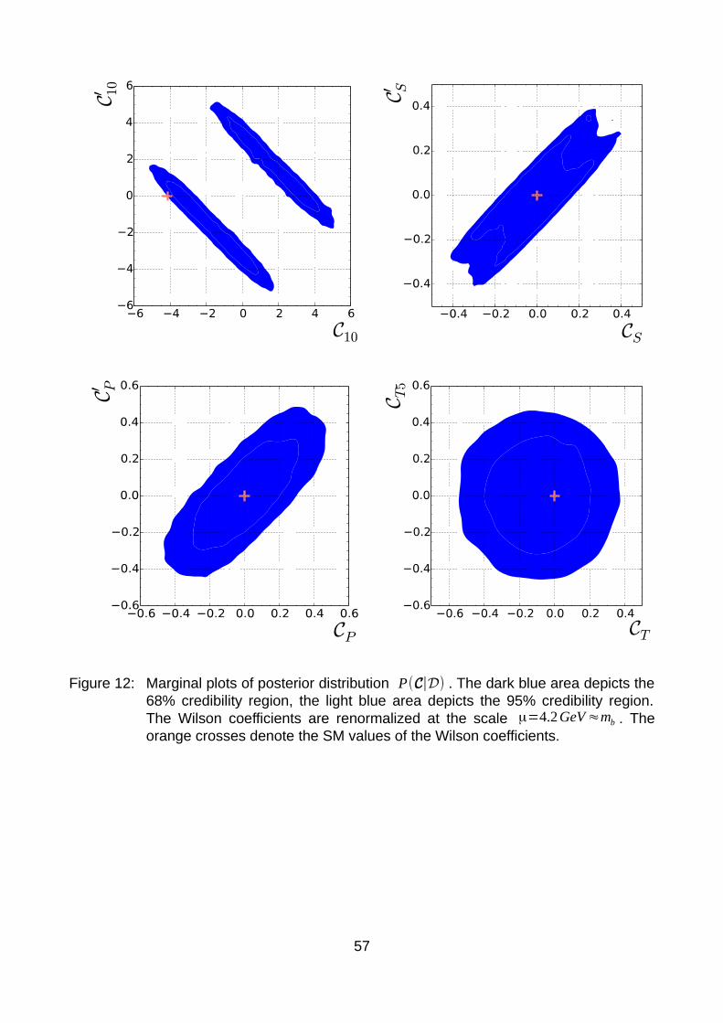
Figure 12: Marginal plots of posterior distribution P(C∣D) . The dark blue area depicts the 68% credibility region, the light blue area depicts the 95% credibility region. The Wilson coefficients are renormalized at the scale μ=4.2GeV ≈mb . The orange crosses denote the SM values of the Wilson coefficients.

57

Figure 13: Marginal plots of posterior distribution P(C∣D) . The dark blue area depicts the 68% credibility region, the light blue area depicts the 95% credibility region. The Wilson coefficients are renormalized at the scale μ=4.2GeV ≈mb . The orange crosses denote the SM values of the Wilson coefficients.

58

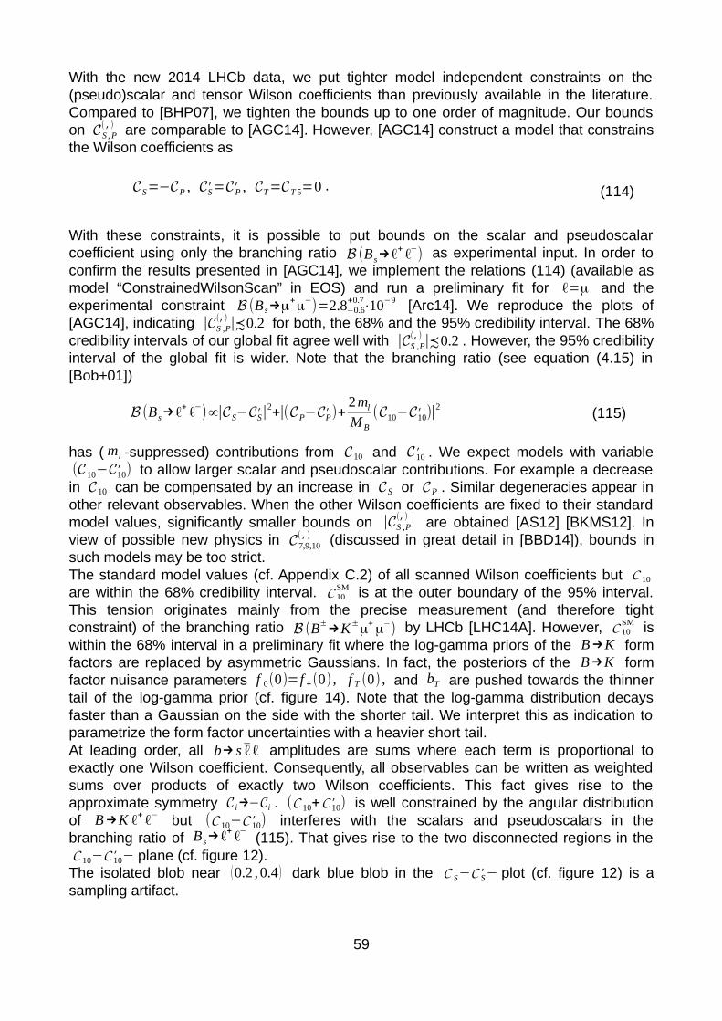
With the new 2014 LHCb data, we put tighter model independent constraints on the (pseudo)scalar and tensor Wilson coefficients than previously available in the literature. Compared to [BHP07], we tighten the bounds up to one order of magnitude. Our bounds on C S , P

(,) are comparable to [AGC14]. However, [AGC14] construct a model that constrains the Wilson coefficients as

C S=−CP , CS,=CP

, , CT=CT 5=0 . (114)

With these constraints, it is possible to put bounds on the scalar and pseudoscalar coefficient using only the branching ratio B (B s→ℓ+ ℓ−) as experimental input. In order to confirm the results presented in [AGC14], we implement the relations (114) (available as model “ConstrainedWilsonScan” in EOS) and run a preliminary fit for ℓ=μ and the experimental constraint B (B s→μ

+μ

−)=2.8−0.6

+0.7⋅10−9 [Arc14]. We reproduce the plots of

[AGC14], indicating |CS ,P(,)

|≾0.2 for both, the 68% and the 95% credibility interval. The 68% credibility intervals of our global fit agree well with |CS ,P

(,)|≾0.2 . However, the 95% credibility

interval of the global fit is wider. Note that the branching ratio (see equation (4.15) in [Bob+01])

B (B s→ℓ+ ℓ−)∝|C S−CS,|

2+|(CP−CP

,)+

2ml

MB

(C10−C10,

)|2

(115)

has ( ml -suppressed) contributions from C 10 and C 10, . We expect models with variable

(C 10−C10,

) to allow larger scalar and pseudoscalar contributions. For example a decrease in C 10 can be compensated by an increase in C S or CP . Similar degeneracies appear in other relevant observables. When the other Wilson coefficients are fixed to their standard model values, significantly smaller bounds on |CS ,P

(,)| are obtained [AS12] [BKMS12]. In

view of possible new physics in C 7,9,10(,) (discussed in great detail in [BBD14]), bounds in

such models may be too strict.The standard model values (cf. Appendix C.2) of all scanned Wilson coefficients but C 10 are within the 68% credibility interval. C 10

SM is at the outer boundary of the 95% interval. This tension originates mainly from the precise measurement (and therefore tight constraint) of the branching ratio B (B±

→K±μ

+μ

−) by LHCb [LHC14A]. However, C 10

SM is within the 68% interval in a preliminary fit where the log-gamma priors of the B →K form factors are replaced by asymmetric Gaussians. In fact, the posteriors of the B →K form factor nuisance parameters f 0(0)=f +(0) , f T (0) , and bT are pushed towards the thinner tail of the log-gamma prior (cf. figure 14). Note that the log-gamma distribution decays faster than a Gaussian on the side with the shorter tail. We interpret this as indication to parametrize the form factor uncertainties with a heavier short tail.At leading order, all b→ s ℓ ℓ amplitudes are sums where each term is proportional to exactly one Wilson coefficient. Consequently, all observables can be written as weighted sums over products of exactly two Wilson coefficients. This fact gives rise to the approximate symmetry C i→−Ci . (C 10+C 10

,) is well constrained by the angular distribution

of B →K ℓ+ ℓ− but (C 10−C 10,

) interferes with the scalars and pseudoscalars in the branching ratio of B s→ℓ+ ℓ− (115). That gives rise to the two disconnected regions in the C 10−C 10

,− plane (cf. figure 12).

The isolated blob near (0.2 ,0.4 ) dark blue blob in the C S−C S,− plot (cf. figure 12) is a

sampling artifact.

59

Figure 14: The nuisance parameters describing the B →K form factors are pushed towards the thinner tail of the log-gamma prior. This effect is most clearly visible in f T (0) . The dashed line shows the prior, the solid line shows the posterior. The dark and light blue regions indicate the 68% and the 95% credibility interval, respectively.

Unlike in the analogous C 7 ,9 , 10(,) -fits [BBD14], the subleading B →K * parameters exhibit no

recognizable deviation from the prior, probably because we only include the branching ratio B (B0

→K *0μ

+μ

−) instead of the full angular distribution (cf. chapter 6.2.1). However,

the nuisance parameter Λ that parametrizes the unknown 1/mb corrections to the B →K form-factor relations at large recoil (cf. chapter 6.2.2) is pulled towards negative values (figure 15). Its posterior is centered at -0.5. Λ=0 , corresponding to negligible subleading corrections, is at the boundary of the 95% posterior credibility interval. In the model with SM-valued Wilson coefficients (model SM ), Λ=0 is even outside the 99.7% (3σ) interval.

60

f T (0)

Figure 15: Subleading contributions to the 1/mb expansion of the amplitude B →K ℓ+ ℓ− , see section 6.2.2. The dashed line shows the prior, the solid line shows the posterior. The dark and light blue regions indicate the 68% and the 95% credibility intervals.

With the findings above, we conclude that a better understanding of the form factors is needed. In particular, we see indications for sizable contributions beyond the well established QCDF at large recoil. This is further discussed by Jäger and Camalich [JC14]. To summarize, more precise theory calculations are needed in order to distinguish between theory uncertainties and new physics [BBD14] [JC14].

The two evidences ZEFT and ZSM are:

ZSM =(4.40±0.02 )⋅10114 , ZEFT=(4.76±0.05 )⋅10108 , (116)

resulting in a Bayes factor of

ZSM /ZEFT≈9.24⋅105 . (117)

Note that the evidence ZEFT depends on the prior range described by the parameters ai in equation (107). Each of the priors P0(Ci) contributes with a factor of (2ai)

−1 to the

61

Λ[GeV ]

evidence. In the following, we investigate the sensitivity of ZEFT to the prior ranges. We define the model EFT ' just like the model EFT but with a tightened prior

P0,(Ci)={(2ai

,)−1 if Ci∈[−ai

,,+a i

,]

0 elsewhere a i

,={

4 if C i∈{C 10 ,C 10,

}

0.3 if C i∈{CS(,) ,CP

( ,) ,CT ,CT 5}(118)

for the Wilson coefficients. The smaller ranges are chosen such that they cover the corresponding 1D 68% credibility intervals and part of the 1D 95% intervals; i.e. we choose the prior ranges such that they only cover important regions. The idea is to ensure that the model EFT ' is not rejected because of too large a parameter volume. We can estimate the evidence ZEFT ' by

ZEFT '=∫ dθ P(D∣O(θ), EFT ')P0(θ ,EFT ')

=∫dθ 1EFT ' (θ)P (D∣O(θ) ,EFT)P0(θ ,EFT)P0(θ ,EFT ' )

P0(θ ,EFT )

≤∫dθ P(D∣O(θ) ,EFT) P0(θ ,EFT)P0(θ ,EFT ')

P0(θ ,EFT)

=ZEFT

P0(θ ,EFT ' )

P0(θ ,EFT)≈1.67⋅10114 ,

(119)

where 1EFT ' denotes the indicator function of the allowed parameter values in the model EFT ' . The prior ratio P0(θ ,EFT ' )/P0(θ ,EFT) reduces to ∏Ci

P0'(Ci)/ P0(C i)=(8 /4)

2

⋅(2/0.3)6≈350,000 since the prior over the nuisance parameters is unchanged. The

numerical values are read off from (107) and (118). Since even with the tighter priors the Bayes factor is less than one (to be precise ≤0.38 ), we conclude that the data do not favor the new-physics model. However, if we impose a strong enough prior in favor of new physics, the posterior odds might still favor the model with new physics. As motivated in the introduction, there undoubtedly are phenomena that cannot be explained by the SM and we therefore should find deviations from the SM at some point.The observables of rare B meson decays seem to be well described by the models EFT and SM . In both models, all pull values (see chapter 7.3 in [Bea12]) are below 2σ .

6.4 Sampling performance

In this section, we evaluate the new algorithm that we present in chapter 5. All statements in this section refer to the algorithm's performance to sample from the posterior distribution P(C ,νth∣D ,EFT) unless stated otherwise.

The Markov chain prerun (cf. chapter 5.1) is performed with the following parameter settings: We run 10 Markov chains, each for 103,000 steps. We discard the first 3,000 samples immediately after creation as part of the burn-in. In particular, these 3,000 samples do not enter the first self-adaptation. For the remaining 105 samples, we run the self-adaptation after every 5,000th sample. Another 10,000 of these samples are deleted as burn-in. We use a Gaussian proposal with an initially diagonal covariance matrix. We do not use the initialization suggested in equation (3.22) of [Bea12]. Instead, we set the

62

proposal variance to 0.01 for the Wilson coefficients. For the nuisance parameters that have an informative prior, we set 10−4

⋅1 /2⋅( σupper+σ lower ) where σupper and σlower denote the upper and lower uncertainties of the prior. That setting is actually an unnoticed bug. The initial proposal variance suggested in equation (3.22) of [Bea12] would be (1/2⋅( σupper+σlower ))

2; i.e. we accidentally miss the square. The prefactor 10−4 is needed

with the faulty initialization because otherwise the proposal is so wide that only points outside the important regions are proposed. Despite of this bug, the self-adaptive Markov chains produce reliable samples. This indicates that MCMC is robust against poor parameter settings.For comparison, we run hierarchical clustering and the variational-Bayes algorithm to obtain a first proposal for importance sampling (cf. chapter 5.2). We thin the MC samples that we plug into VB by a factor of 50. The chain grouping by R value results in two groups - the two stripes that are nicely visible in the upper left plot of figure 12. Hierarchical clustering achieves P =0.225% and ESS=0.065% (estimated from 100,800 samples) while VB yields a ten-times higher perplexity and doubles the ESS (cf. table 6). The parameter settings are Kg=50 for HC and Kg=10 for VB. We do not try other values of

Kg but in particular the old algorithm is very sensitive to that parameter. In fact, none of the 100 initial output components for HC is pruned during the HC run. In contrast, the number of components is reduced from 20 to 12 by VB. We run three further proposal updates (cf. chapter 5.3) but with the variational-Bayes algorithm only. For each proposal update with VB, we combine all samples from earlier proposals as described in [Cor+12] (see also chapter 5.4) and impose the VB posterior of the MCMC data as informative prior. Since there obviously are two disconnected regions (figure 12, upper left plot), we set the VB hyperparameters α0k to the “uninformative” value 10−5 (see chapter 5.3.2 for a discussion of the hyperparameter settings). Empirical perplexity and effective sample size of the remaining proposals are listed in table 6. The variational-Bayes algorithm reduces the number of components to 4 during the first further proposal update. In the two remaining updates, the number of components does not change any more.

P [%]

ESS [%]

number of samples

first proposal 2.32 0.13 302,400

second proposal 2.30 0.22 201,600

third proposal 4.89 0.51 453,600

combination 6.11 1.17 957,600

Table 6: Perplexity ( P ) and Effective Sample Size (ESS) of the samples used for the plots and for calculating the Bayes factor in chapter 6.3.

The plots in this chapter are drawn with the combined importance-weighted samples (957,600 samples in total). The combined weights are free of severe outliers such that cropping (see chapter 4.3.3.1 in [Bea12]) becomes unnecessary. This is a major improvement as outliers are a major difficulty in the importance-sampling approach. Nevertheless, when only regarding the samples from a single proposal (without combination à la Cornuet et al. [Cor+12]) outliers still occur. We can see the reduction of

63

outliers in the effective samples sizes: The last individual proposal alone achieves the highest ESS=0.51% , whereas the ESS of the combination is more than twice as large (cf. table 6).However, the effective number of samples N eff ≡ESS⋅N , where N denotes the total number of importance samples, is the important quantity that determines the accuracy of integral estimates and the quality of plots. As can be seen in (75), a worse proposal can always (at least in theory) be compensated by more samples. In total, we gain roughly N eff =11,000 effective samples for approximately two million calls to the posterior (one

million MCMC samples plus one million importance samples).Note that the old algorithm needs many more function evaluations. In table 7.4 of [Bea12], we see that PMC must be run at least ten times until convergence on 18 to 31 dimensional similar problems. With O(50) components and N c≥3,000 (cf. table 7.4 in [Bea12]), more than 10⋅50⋅3,000=1.5⋅106 importance samples are drawn but not merged into the final output. Another one to five million samples are drawn during MCMC. Thus, the old algorithm needs more than 2.5 million calls to the target before the first sample that enters the final output can be drawn. The output only consists of the additionally drawn final two million importance samples.The effective sample sizes reached after typically much more than two million calls to the target vary between 6% and 45% (table 7.4 in [Bea12]). In contrast, the proposal for our 29 dimensional fit of only the nuisance parameters (model SM ) already reaches an ESS of 48% using just the about one million samples from MCMC.Note that all distributions considered in table 7.4 of [Bea12] are at most 31 dimensional. Due to the curse of dimensionality, our 37 dimensional distribution P(C ,νth∣D ,EFT) can less well be approximated by a Gaussian mixture which results in a lower ESS. We expect that the old algorithm would, just like our enhanced version, only yield an ESS at the percent level. However, the old algorithm would need millions of samples to generate the proposal. Furthermore, the old algorithm would discard the millions of learning samples and need another final sampling run.

64

7 ConclusionWe tighten earlier data-driven constraints on the scalar, pseudoscalar, and tensor Wilson coefficients in an effective b→ s theory. The angular observables of B →K ℓ+ ℓ− and the branching fraction of B s→ℓ+ ℓ− are particularly sensitive to these coefficients since the vectorial couplings of the SM are helicity suppressed. We are, to our knowledge, the first to constrain all of C 10

(,) , C S(,) ,C P

(,), C T , and C T 5 simultaneously in a global fit. We extend previous work [AGC14] [AS12] [BKMS12] where more restricted models and, except for [AGC14], older data are considered. In contrast, we consider all Wilson coefficients as a-priori independent. As a consequence, we need more observables in order to constrain the additional degrees of freedom and thus exploit the latest measurements.Moreover, we account for theory uncertainties, in particular the not-well-known hadronic form factors, in an atypically sophisticated way. This is naturally achieved in the Bayesian approach by the introduction of nuisance parameters. To better constrain the (pseudo)scalar and tensor Wilson coefficients, it would be desirable to have B →K * angular analyses that do not assume these coefficients to vanish.We argue that the current theoretical approach needs a refinement to distinguish between new physics and theory uncertainties. In particular, we see indications of sizable 1/mb corrections to the well established QCDF approach. Furthermore, the exclusion of C 10

SM at 2σ only arises when log-gamma distributions instead of asymmetric Gaussians are used to parametrize the B →K form-factor prior. We conclude that the shorter tails of the log-gamma distributions decay too fast and hence introduce that unexpected deviation.We further point out that the bounds on C S , P

(,) , C T , and C T 5 are less strict in models with variable C 10

(,) compared to models that fix C 10(,)

=C 10(,)SM . We expect even looser bounds in

models that additionally allow non-SM values for C 7(,) and C 9

(,) .The inferred (pseudo)scalar and tensor Wilson coefficients agree well (within the 68% credibility interval) with the standard model prediction. The Bayes factors favor the standard model SM over generic new-physics models EFT ( ' ) .

To run the global fit at all, we have to develop an algorithm that can sample and integrate a multimodal and 37 dimensional nonnegative function. We present an enhanced version of the algorithm suggested in [Bea12] [BC13]. We find that the combination of Markov chains, the variational-Bayes algorithm, and importance sampling can efficiently sample and integrate O(40) dimensional and multimodal functions even when only little analytical knowledge is available.We show two possibilities to improve the proposal density generated from the Markov chain samples compared to [Bea12] [BC13]: First, using VB instead of the hierarchical clustering results in an algorithm that reliably reduces unnecessary components. On the contrary, the number of components has to be carefully tuned in the old algorithm and its automatic determination is considered as an open question in [Bea12]. Second, running multiple PMC updates with a very large number of Markov chain samples can result in a better proposal than obtained with VB. Nevertheless, we recommend to rather use VB because it is more robust against too few MCMC samples. In addition, the variational-Bayes algorithm comes with an advantage for further proposal updates: It is possible to include the information acquired from the Markov chains. In contrast to PMC, the variational-Bayes algorithm takes a prior distribution into account. We can therefore consistently provide VB with an informative prior that summarizes exactly the information gained from MCMC.

65

With our improved post processing of the Markov chain samples, the further proposal updates become less important. However, we still achieve an increase in ESS by a factor of five after two further proposal updates in the global fit.We gain another factor of two in ESS when we merge the samples of all intermediate proposals as suggested in [Cor+12]. In addition, the combination of samples brings several more benefits: First, it significantly reduces outliers. In fact, we do not need to crop any outliers, which is a major advantage over the algorithm considered in [Bea12] [BC13]. Second, the samples drawn for further proposal updates can be merged into the final output. Without the ability to combine samples, these would have to be discarded like in the original algorithm. Third, the combination stabilizes further proposal updates since all previously drawn importance samples are directly included, not only the latest ones.We expect that our current approach works, for real-life problems, in up to O(40) dimensions; i.e. we believe that we already drive our algorithm to its maximum. Our approach is based on approximating the target function and it is known that an error of ϵ in each dimension enters the importance weights as (1+ϵ)

d . Nonetheless, in the regime of ≾40 dimensions, we provide a generic algorithm to sample and integrate an in principle arbitrary function. In particular, we provide an algorithm that can cope with multimodality in high dimensions. It shall be emphasized that there is no standard integration or sampling algorithm for high-dimensional and multimodal target functions yet.We apply the variational-Bayes approach with Gaussian mixtures so far. If we revive the cropping and replace the Gaussians by Student's T distributions, up to O(50) dimensional problems should become tractable. The hope with Student's T distribution is that outliers are reduced by the heavier tails, also for low-dimensional targets that decay slower than a Gaussian. We therefore develop an extension to existing variational-Bayes approaches with Student's T mixture densities. We are, to our knowledge, the first to discuss that method with the full conjugate prior for the degree-of-freedom parameter. We derive the update equations up to integrals over the degree-of-freedom prior. These 1D integrals can, taking care of several pitfalls, be computed numerically; i.e. we provide an implementation-ready description. The conjugate prior that naturally arises does not belong to any well known class of probability distributions. We further show that the conjugate dof-prior is not unique. The development of analytic expressions for the yet unsolved integrals is postponed to future work.Besides the algorithm best suited to our problem, we discuss alternatives for other kinds of problems. In chapter 5.2.4.1, we show that our modified usage of PMC (cf. chapter 5.2.2) can achieve higher ESS than HC or VB but only if enough Markov chain samples are provided. Since for us “enough” would mean “way too many”, we do not follow that approach. However, if it is fast to evaluate the target distribution or if the effective number of samples N eff ≡ESS⋅N is considered less important than the ESS, PMC can be the better choice over VB. In case of a low-dimensional and very-fast-to-evaluate target distribution, meaning that PMC or VB updates take much longer than calls to the target, it might be sensible to stay with the hierarchical clustering.We provide an open source implementation of the aforementioned algorithms in the python package pypmc (cf. Appendix B).

66

Appendix

A Probability DistributionsIn this section, we define the probability distributions used throughout this work. In this chapter we consistently denote the dimensionality with d . Bold Symbols are used for vector or matrix variables whereas normal printed symbols denote real numbered variables.

A.1 Gauss / Normal

In physics, the univariate Normal distribution is widely used to approximate uncertainties. Whenever a physicist writes a=b±c it is implied that the variable a has been measured to take the value b with an uncertainty c . Translated into the Bayesian framework that means a is a random variable distributed according to the univariate Normal distribution N (a∣b , c) . The Normal distribution also arises as limiting distribution in the central limit theorem.The two names “Normal” and “Gaussian” distribution are commonly considered equivalent.The parameters of a Gaussian are the mean value μ∈ℝ

d and the covariance matrix

Σ∈ℝd×d , positivedefinite where d denotes the dimensionality. The support is x∈ℝ

d .

PDF: N ( x∣μ , Σ)≡(2π )−

d2|Σ|

−12 exp(−1

2(x−μ)

TΣ

−1(x−μ)) (120)

mode: x=μ (121)

mean: E[ x]=μ (122)

cov.: cov [ x]=Σ (123)

The univariate normal distribution (d=1 ) is usually parametrized in terms of the standard deviation σ≡√Σ ∈ℝ

+ instead of the covariance. In order to avoid confusion, we clarify that we mean

N ( x∣μ ,σ)≡1

√2π σe

−(x−μ )

2

2σ2

(124)

whenever we talk about the univariate Normal distribution.

A.2 Student's T

Student's T distribution is similar to the Normal distribution but has heavier tails. The tail probability mass is adjusted by an additional parameter compared to the Gaussian; the degrees of freedom ν>0 . Like the Gaussian, Student's T distribution takes the parameters μ∈ℝ

d and Σ∈ℝd×d , positive definite . Note that Σ is NOT the covariance matrix in this case (128).

67

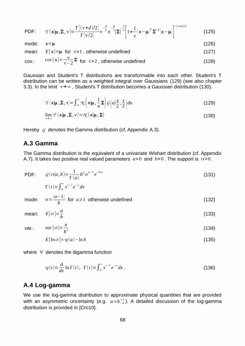
PDF: T (x∣μ ,Σ , ν)≡Γ [(ν+d )/2 ]

Γ [ ν/2 ]ν

−d2 π

−d2|Σ|

−12 [1+

1

ν( x−μ )

TΣ

−1 (x−μ )]−(ν+d )/2

(125)

mode: x=μ (126)

mean: E[ x]=μ for ν>1 , otherwise undefined (127)

cov.: cov [ x]= νν−2

Σ for ν>2 , otherwise undefined (128)

Gaussian and Student's T distributions are transformable into each other. Student's T distribution can be written as a weighted integral over Gaussians (129) (see also chapter 3.3). In the limit ν→∞ , Student's T distribution becomes a Gaussian distribution (130).

T ( x∣μ ,Σ , τ )=∫0

∞

N ( x∣μ ,1u

Σ)G (u∣τ2

, τ2 )du (129)

limν→ ∞

T (x∣μ ,Σ ,ν)=N (x∣μ , Σ) (130)

Hereby G denotes the Gamma distribution (cf. Appendix A.3).

A.3 Gamma

The Gamma distribution is the equivalent of a univariate Wishart distribution (cf. Appendix A.7). It takes two positive real valued parameters a>0 and b>0 . The support is σ>0 .

PDF: G (σ∣a ,b)≡1

Γ(a)b

aσ

a−1e

−bσ(131)

Γ( t)≡∫0

∞

x t−1e−x dx

mode: σ=(a−1 )

b for a≥1 otherwise undefined (132)

mean: E[σ ]=ab

(133)

var.: var [σ]=a

b2 (134)

E[ ln σ ]=ψ(a)− ln b (135)

where ψ denotes the digamma function

ψ(t)≡ddx

ln Γ(t) , Γ( t)≡∫0

∞

xt−1

e−x

dx . (136)

A.4 Log-gamma

We use the log-gamma distribution to approximate physical quantities that are provided with an asymmetric uncertainty (e.g. a=b− d

+ c ). A detailed discussion of the log-gamma distribution is provided in [Cro10].

68

PDF: LogGamma ( x∣ν ,λ ,α )≡1

Γ(α)|λ|exp {α ( x−ν

λ )−exp( x−ν

λ )} (137)

x , ν ,λ ∈ℝ , α>0

mode: x=ν−λ lnα (138)

mean: E[ x ]=ν+λ ψ(α) (139)

var.: var [x ]=λ2ψ1(α) (140)

where ψ≡ψ0 denotes the digamma function (136) and ψn ,

ψn(t)≡dn+1

dt n+1 ln Γ(t) , Γ( t)≡∫0

∞

xt−1e−x dx , (141)

denotes the polygamma function.

A.5 Dirichlet

The Dirichlet distribution arises as conjugate prior for the component weights in Gaussian or Student's T mixture models (cf. chapters 3.2 and 3.3). The parameter αk can be interpreted as the number of observed samples from component k . One may expect the component weights to be the self-normalized vector α which is exactly the mean (144). With more observations the uncertainty on the component weights decreases (145).

PDF: Dir (π∣α )≡C (α)∏k=1

K

πkαk−1 (142)

C(α)≡Γ(∑k=1

K

αk)/∏k=1

K

Γ ( αk )

π∈ℝK , 0≤πk≤1, ∑k=1

K

πk=1 , α∈ℝK ,αk>0

mode: πk=(αk−1 ) /(∑k '=1

K

αk'−K ) for αk>1 otherwise undefined (143)

mean: E[π ]=α/∑k=1

K

αk (144)

var.: var [πk ]=

αk (∑k'=1

K

αk '−αk)(∑

k '=1

K

αk ' )2

(∑k '=1

K

αk '+1)(145)

69

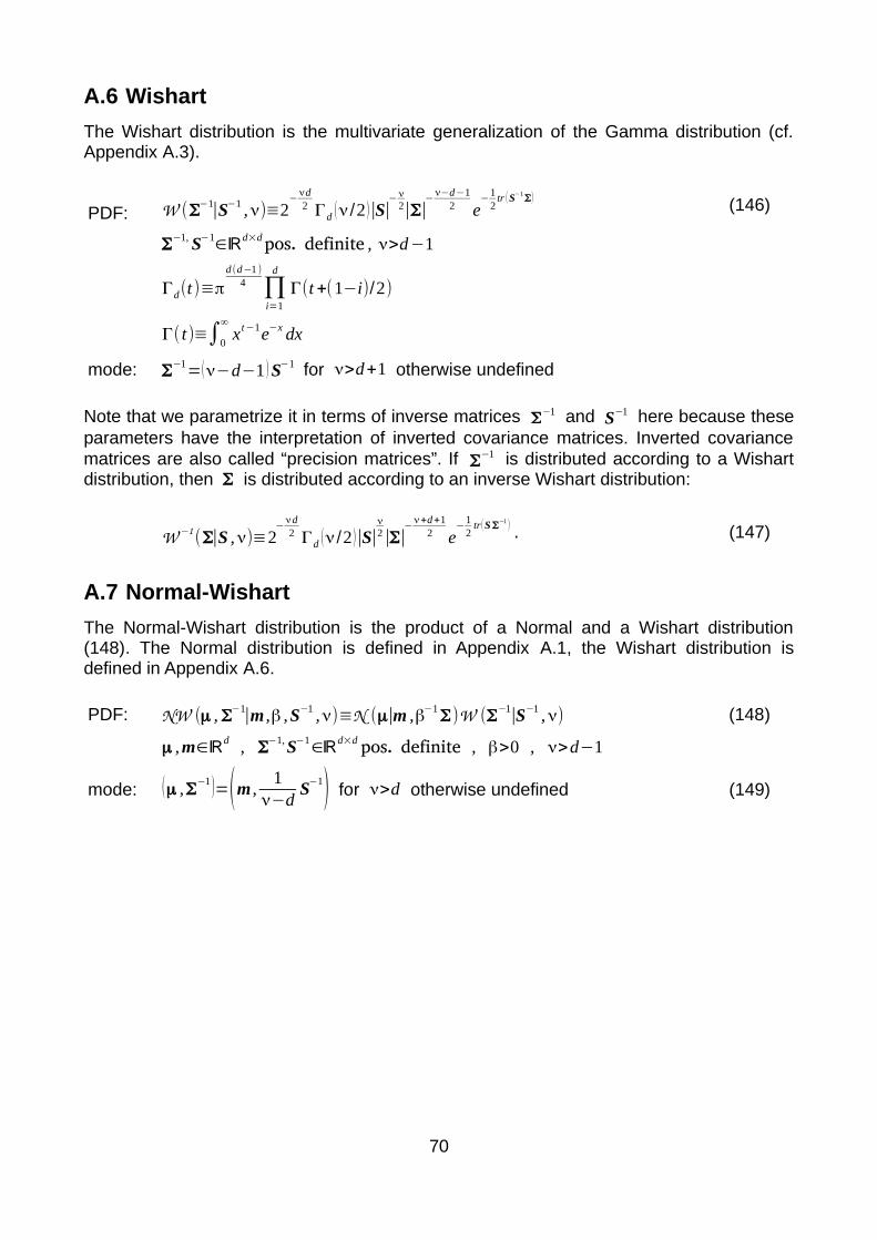
A.6 Wishart

The Wishart distribution is the multivariate generalization of the Gamma distribution (cf. Appendix A.3).

PDF: W (Σ−1∣S−1 ,ν)≡2−

νd2 Γd (ν/2 )|S|

− ν2|Σ|

−ν−d−1

2 e−

12

tr ( S−1Σ) (146)

Σ−1, S−1

∈ℝd×dpos. definite , ν>d−1

Γd(t)≡πd (d−1 )

4 ∏i=1

d

Γ(t +(1−i)/2)

Γ( t)≡∫0

∞

x t−1e−x dx

mode: Σ−1

=(ν−d−1 ) S−1 for ν>d+1 otherwise undefined

Note that we parametrize it in terms of inverse matrices Σ−1 and S−1 here because these

parameters have the interpretation of inverted covariance matrices. Inverted covariance matrices are also called “precision matrices”. If Σ

−1 is distributed according to a Wishart distribution, then Σ is distributed according to an inverse Wishart distribution:

W −1(Σ∣S ,ν)≡2

−νd2 Γd (ν/2 )|S|

ν2|Σ|

−ν+d+1

2 e−

12

tr ( S Σ−1 ) . (147)

A.7 Normal-Wishart

The Normal-Wishart distribution is the product of a Normal and a Wishart distribution (148). The Normal distribution is defined in Appendix A.1, the Wishart distribution is defined in Appendix A.6.

PDF: NW (μ , Σ−1

∣m ,β ,S−1 ,ν)≡N (μ∣m ,β−1Σ)W (Σ

−1∣S−1 ,ν) (148)

μ ,m∈ℝd , Σ

−1,S−1∈ℝ

d×d pos. definite , β>0 , ν>d−1

mode: (μ ,Σ−1 )=(m ,

1ν−d

S−1) for ν>d otherwise undefined (149)

70

B The python package pypmcpypmc explains itself like this:

pypmc is a python package focusing on adaptive importance sampling. It can be used for integration and sampling from a user-defined target density. A typical application is Bayesian inference, where one wants to sample from the posterior to marginalize over parameters and to compute the evidence. The key idea is to create a good proposal density by adapting a mixture of Gaussian or student's t components to the target density. The package is able to efficiently integrate multimodal functions in up to about 30-40 dimensions at the level of 1% accuracy or less. For many problems, this is achieved without requiring any manual input from the user about details of the function.

We originally developed pypmc to test and compare the different proposal updating algorithms presented in chapter 5 during the preparation of this thesis. Releases can be downloaded from the python package index https://pypi.python.org/pypi/pypmc. The full development history is available on github https://github.com/fredRos/pypmc. Detailed installation instructions can be found in the full documentation available online at http://pythonhosted.org/pypmc. The documentation also contains examples that illustrate the usage of the most important functions and classes. In addition, all public methods are documented in the reference guide.pypmc implements self-adaptative Markov chains (cf. chapter 4.1) and importance sampling (cf. chapter 4.2.1) along with the clustering algorithms hierarchical clustering (cf. chapter 5.2.1), variational-Bayes clustering (cf. chapter 3), and PMC (cf. chapter 5.2.2). The posterior distributions of the Wilson coefficients shown in chapter 6.3 have been mapped out with pypmc. With a parallel sampler class it is also possible to run multiple Markov chains or importance sampling on a computing cluster using mpi4py. pypmc was run on C2PAP (http://www.universe-cluster.de/c2pap) for the Wilson coefficient analysis (cf. chapter 6).

C Supplement to chapter 6C.1 The HPQCD form factor constraint

The B →K μ+μ

− form factors in EOS are each parametrized by two nuisance parameters as described in [KMPW10]. The parametrization consists of the form factor at q2

=0 and a slope parameter. We vary their values at q2

=0 ( f T (0) , f 0(0)=f + (0)) and a slope

parameter for each form factor (bT , b0, b+ ) . Recent lattice calculations [HPQCD13] use a different parametrization. To include their result, we draw 50,000 B →K form factor samples using their parametrization (with uncertainties) for the values of q2

=17 GeV 2 , q2=20GeV 2 , and q2

=23GeV 2 . We include the sample mean and covariance (cf. table 7) as Gaussian constraint on the form factors. This constraint is available in [EOS] as “B->K::f_0+f_++f_T@HPQCD-2013A”. The same method is also applied in [BBD14].

71

central values

q2 17 20 23

f 0(q2) 0.616 0.723 0.87

f + (q2) 1.13 1.63 2.68

f T (q2) 1.02 1.47 2.42

covariance matrix

f 0(17) f 0(20) f 0(23) f + (17) f + (20) f + (23) f T (17) f T (20) f T (23)

f 0(17) 0.0303 0.0298 0.0253 0.0231 0.0224 0.0146 0.00544 0.005052 0.00354

f 0(20) 0.0338 0.0321 0.0172 0.0224 0.0163 0.00263 0.00498 0.00587

f 0(23) 0.0400 0.0129 0.0185 0.0232 0.000503 0.00268 0.00494

f + (17) 0.0531 0.0486 0.0250 0.0205 0.0143 0.00499

f + (20) 0.0726 0.0701 0.0146 0.0206 0.0226

f + (23) 0.133 -0.00222 0.0149 0.0341

f T (17) 0.0596 0.0557 0.0475

f T (20) 0.0844 0.105

f T (23) 0.181

Table 7: Reproduced B+→ K+ form factors from [HPQCD13] at q2

=17, 20, 23 GeV 2 ; the GeV 2 is omitted for brevity. This constraint enters the likelihood used in chapter 6 as multivariate Gaussian.

72

C.2 Wilson coefficients – SM prediction

The standard model predicts the following numerical values for the Wilson coefficients:

C 1SM

=−0.291 C 2SM

=+1.01

C 3SM

=−0.00616 C 5SM

=+0.000429

C 4SM

=−0.0873 C 6SM

=+0.00116

C 7SM

=−0.337 C 9

SM=+4.27

C 8

SM=−0.183 C 10

SM=−4.17

Table 8: Standard model predictions for the Wilson coefficients.

Coefficients of operators not listed in table 8 but in equation (93) or (94) are zero in the standard model. When we state that we “keep some Wilson coefficient fixed at its standard model value”, we mean that we insert the value stated above. These values are taken from the file “parameters.cc” in [EOS]. For the theoretical calculation see [BMU00].

C.3 Internal EOS report

In the EOS python interface, the log-posterior (cf. equation (103)) is implemented as callable class named “Analysis”. The following is an excerpt of the string representation of the “Analysis” instance used for the model EFT . The model SM uses the same constraints and parameters except for the Wilson coefficients. With the information provided below, it is possible to reconstruct the “Analysis” instance we use.

Constraints (25): B^0_s->mu^+mu^-::BR@CMS-LHCb-2014 B^+->K^+mu^+mu^-::BR[15.00,22.00]@LHCb-2014 B^+->K^+mu^+mu^-::A_FB[15.00,22.00]@LHCb-2014 B^+->K^+mu^+mu^-::F_H[15.00,22.00]@LHCb-2014 B^+->K^+mu^+mu^-::BR[14.18,16.00]@CDF-2012 B^+->K^+mu^+mu^-::BR[16.00,22.86]@CDF-2012 B^+->K^+mu^+mu^-::A_FB[14.18,16.00]@CDF-2012 B^+->K^+mu^+mu^-::A_FB[16.00,22.86]@CDF-2012 B^+->K^+mu^+mu^-::BR[1.10,6.00]@LHCb-2014 B^+->K^+mu^+mu^-::A_FB[1.10,6.00]@LHCb-2014 B^+->K^+mu^+mu^-::F_H[1.10,6.00]@LHCb-2014 B^+->K^+mu^+mu^-::BR[1.00,6.00]@CDF-2012 B^+->K^+mu^+mu^-::A_FB[1.00,6.00]@CDF-2012 B^0->K^*0mu^+mu^-::BR[1.00,6.00]@CDF-2012 B^0->K^*0mu^+mu^-::BR[14.18,16.00]@CDF-2012 B^0->K^*0mu^+mu^-::BR[16.00,19.21]@CDF-2012 B^0->K^*0mu^+mu^-::BR[1.00,6.00]@CMS-2013A

73

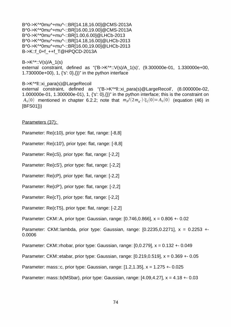
B^0->K^*0mu^+mu^-::BR[14.18,16.00]@CMS-2013A B^0->K^*0mu^+mu^-::BR[16.00,19.00]@CMS-2013A B^0->K^*0mu^+mu^-::BR[1.00,6.00]@LHCb-2013 B^0->K^*0mu^+mu^-::BR[14.18,16.00]@LHCb-2013 B^0->K^*0mu^+mu^-::BR[16.00,19.00]@LHCb-2013 B->K::f_0+f_++f_T@HPQCD-2013A

B->K^*::V(s)/A_1(s)external constraint, defined as “('B->K^*::V(s)/A_1(s)', (9.300000e-01, 1.330000e+00, 1.730000e+00), 1, {'s': 0},{})” in the python interface

B->K^*ll::xi_para(s)@LargeRecoilexternal constraint, defined as “('B->K^*ll::xi_para(s)@LargeRecoil', (8.000000e-02, 1.000000e-01, 1.300000e-01), 1, {'s': 0},{})” in the python interface; this is the constraint on A0(0) mentioned in chapter 6.2.2; note that mB/(2mK*)⋅ξ∥(0)= A0(0) (equation (46) in

[BFS01]))

Parameters (37):

Parameter: Re{c10}, prior type: flat, range: [-8,8]

Parameter: Re{c10'}, prior type: flat, range: [-8,8]

Parameter: Re{cS}, prior type: flat, range: [-2,2]

Parameter: Re{cS'}, prior type: flat, range: [-2,2]

Parameter: Re{cP}, prior type: flat, range: [-2,2]

Parameter: Re{cP'}, prior type: flat, range: [-2,2]

Parameter: Re{cT}, prior type: flat, range: [-2,2]

Parameter: Re{cT5}, prior type: flat, range: [-2,2]

Parameter: CKM::A, prior type: Gaussian, range: [0.746,0.866], x = 0.806 +- 0.02

Parameter: CKM::lambda, prior type: Gaussian, range: [0.2235,0.2271], x = 0.2253 +- 0.0006

Parameter: CKM::rhobar, prior type: Gaussian, range: [0,0.279], x = 0.132 +- 0.049

Parameter: CKM::etabar, prior type: Gaussian, range: [0.219,0.519], x = 0.369 +- 0.05

Parameter: mass::c, prior type: Gaussian, range: [1.2,1.35], x = 1.275 +- 0.025

Parameter: mass::b(MSbar), prior type: Gaussian, range: [4.09,4.27], x = 4.18 +- 0.03

74

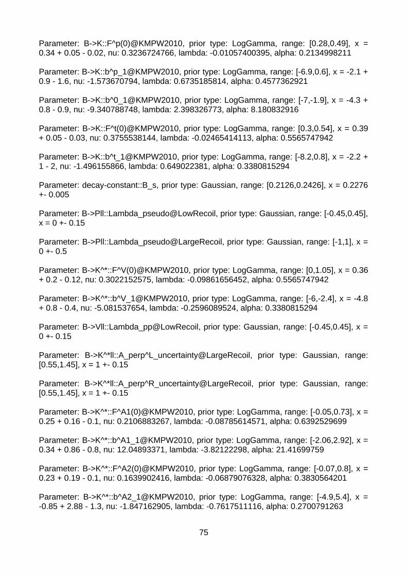
Parameter: B->K::F^p(0)@KMPW2010, prior type: LogGamma, range: [0.28,0.49], x = 0.34 + 0.05 - 0.02, nu: 0.3236724766, lambda: -0.01057400395, alpha: 0.2134998211

Parameter: B->K::b^p_1@KMPW2010, prior type: LogGamma, range: [-6.9,0.6], x = -2.1 + 0.9 - 1.6, nu: -1.573670794, lambda: 0.6735185814, alpha: 0.4577362921

Parameter: B->K::b^0_1@KMPW2010, prior type: LogGamma, range: [-7,-1.9], x = -4.3 + 0.8 - 0.9, nu: -9.340788748, lambda: 2.398326773, alpha: 8.180832916

Parameter: B->K::F^t(0)@KMPW2010, prior type: LogGamma, range: [0.3,0.54], x = 0.39 + 0.05 - 0.03, nu: 0.3755538144, lambda: -0.02465414113, alpha: 0.5565747942

Parameter: B->K::b^t_1@KMPW2010, prior type: LogGamma, range: [-8.2,0.8], x = -2.2 + 1 - 2, nu: -1.496155866, lambda: 0.649022381, alpha: 0.3380815294

Parameter: decay-constant::B_s, prior type: Gaussian, range: [0.2126,0.2426], x = 0.2276 +- 0.005

Parameter: B->Pll::Lambda_pseudo@LowRecoil, prior type: Gaussian, range: [-0.45,0.45], x = 0 +- 0.15

Parameter: B->Pll::Lambda_pseudo@LargeRecoil, prior type: Gaussian, range: [-1,1], x = 0 +- 0.5

Parameter: B->K^*::F^V(0)@KMPW2010, prior type: LogGamma, range: [0,1.05], x = 0.36 + 0.2 - 0.12, nu: 0.3022152575, lambda: -0.09861656452, alpha: 0.5565747942

Parameter: B->K^*::b^V_1@KMPW2010, prior type: LogGamma, range: [-6,-2.4], x = -4.8 + 0.8 - 0.4, nu: -5.081537654, lambda: -0.2596089524, alpha: 0.3380815294

Parameter: B->Vll::Lambda_pp@LowRecoil, prior type: Gaussian, range: [-0.45,0.45], x = 0 +- 0.15

Parameter: B->K^*ll::A_perp^L_uncertainty@LargeRecoil, prior type: Gaussian, range: [0.55,1.45], x = 1 +- 0.15

Parameter: B->K^*ll::A_perp^R_uncertainty@LargeRecoil, prior type: Gaussian, range: [0.55,1.45], x = 1 +- 0.15

Parameter: B->K^*::F^A1(0)@KMPW2010, prior type: LogGamma, range: [-0.05,0.73], x = 0.25 + 0.16 - 0.1, nu: 0.2106883267, lambda: -0.08785614571, alpha: 0.6392529699

Parameter: B->K^*::b^A1_1@KMPW2010, prior type: LogGamma, range: [-2.06,2.92], x = 0.34 + 0.86 - 0.8, nu: 12.04893371, lambda: -3.82122298, alpha: 21.41699759

Parameter: B->K^*::F^A2(0)@KMPW2010, prior type: LogGamma, range: [-0.07,0.8], x = 0.23 + 0.19 - 0.1, nu: 0.1639902416, lambda: -0.06879076328, alpha: 0.3830564201

Parameter: B->K^*::b^A2_1@KMPW2010, prior type: LogGamma, range: [-4.9,5.4], x = -0.85 + 2.88 - 1.3, nu: -1.847162905, lambda: -0.7617511116, alpha: 0.2700791263

75

Parameter: B->Vll::Lambda_0@LowRecoil, prior type: Gaussian, range: [-0.45,0.45], x = 0 +- 0.15

Parameter: B->Vll::Lambda_pa@LowRecoil, prior type: Gaussian, range: [-0.45,0.45], x = 0 +- 0.15

Parameter: B->K^*ll::A_0^L_uncertainty@LargeRecoil, prior type: Gaussian, range: [0.55,1.45], x = 1 +- 0.15

Parameter: B->K^*ll::A_0^R_uncertainty@LargeRecoil, prior type: Gaussian, range: [0.55,1.45], x = 1 +- 0.15

Parameter: B->K^*ll::A_par^L_uncertainty@LargeRecoil, prior type: Gaussian, range: [0.55,1.45], x = 1 +- 0.15

Parameter: B->K^*ll::A_par^R_uncertainty@LargeRecoil, prior type: Gaussian, range: [0.55,1.45], x = 1 +- 0.15

76

List of abbreviationscov: covariancedof: degrees of freedomEFT: effective field theoryEM: expectation maximizationESS: effective sample sizeFCNC: flavor changing neutral currentHMC: Hamiltonian Monte CarloHC: hierarchical clusteringiid: independent and identically distributedIS: importance samplingKL: Kullback-Leibler divergenceMC: Markov chainPDF: probability density functionPMC: Population Monte CarloQCD quantum chromodynamicsQCDF QCD factorizationQFT: quantum field theorySM: standard modelvar: varianceVB: variational Bayes

77

Bibliography[AGC14]: Alonso, R. and Grinstein, B. and Camalich, J. M.; SU(2)×U(1) gauge

invariance and the shape of new physics in rare B decays; Physical Review Letters, Volume 113, pp. 241802, 2014DOI: 10.1103/PhysRevLett.113.241802

[Arc14]: Archilli, F.; B s , d→μ+μ− (experiment); The 8th International Workshop on the CKM Unitary Triangle, 2014http://indico.cern.ch/event/253826/session/6/contribution/27

[AS12]: Altmannshofer, W. and Straub, D. M.; Cornering New Physics in b→ s Transitions; Journal of High Energy Physics, 2012DOI: 10.1007/JHEP08(2012)121

[AS72]: Abramowitz, M. and Stegun, I. A.; Handbook of Mathematical Functions; Wiley New York 1972ISBN: 0-486-61272-4http://people.maths.ox.ac.uk/~macdonald/aands/index.html

[ATLAS12]: Aad, G. et al.; Observation of a new particle in the search for the Standard Model Higgs boson with the ATLAS detector at the LHC; Physics Letters B, Volume 716, Issue 1, pp. 1-29, 2012DOI: 10.1016/j.physletb.2012.08.020

[AV07]: Archambeau, C. and Verleysen, M.; Robust Bayesian clustering; Neural Networks, Vol. 20, Issue 1, pp. 129-138, 2007DOI: 10.1016/j.neunet.2006.06.009

[BaBar12A]: Lees, J. P. et al.; Measurement of branching fractions and rate asymmetries in the rare decays B →K (*)ℓ+ℓ− ; Phys. Rev. D 86, pp. 032012, 2012DOI: 10.1103/PhysRevD.86.032012

[Babar12B]: Ritchie, J. L.; Angular Analysis of B →K (*)ℓ+ℓ− in BABAR; 2012arXiv:1301.1700

[BB98]: Ball, P. and Braun, V.M.; Exclusive Semileptonic and Rare B-Meson Decays in QCD; Physical Review D, Volume 58, pp. 094016, 1998DOI: 10.1103/PhysRevD.58.094016

[BBD14]: Beaujean, F. and Bobeth, C. and van Dyk, D.; Comprehensive Bayesian analysis of rare (semi)leptonic and radiative B decays; The European Physical Journal C, pp. 2897, 2014DOI: 10.1140/epjc/s10052-014-2897-0

[BBDW12]: Beaujean, F. and Bobeth, C. and van Dyk, D. and Wacker, C.; Bayesian Fit of Exclusive b→ s ℓ ℓ decays: The Standard Model Operator Basis; Journal of High Energy Physics, 2012DOI: 10.1007/JHEP08(2012)030

78

[BC13]: Beaujean, F. and Caldwell, A.; Initializing adaptive importance sampling with Markov chains; 2013arXiv:1304.7808

[Bea12]: Beaujean, F.; A Bayesian analysis of rare B decays with advanced Monte Carlo methods; Ph.D. Thesis, Technische Universität München, 2012http://nbn-resolving.de/urn/resolver.pl?urn:nbn:de:bvb:91-diss-20121114-1115832-1-8

[Belle09]: Wei, J.-T. et al.; Measurement of the Differential Branching Fraction and Forward-Backword Asymmetry for B →K (*)ℓ+ℓ− ; Phys. Rev. Lett. 103, pp. 171801, 2009DOI: 10.1103/PhysRevLett.103.171801

[BF00]: Beneke, M. and Feldmann, T.; Symmetry-breaking corrections to heavy-to-light B meson form factors at large recoil; Nuclear Physics B, Volume 592, Issues 1-2, pp. 3-34, 2000DOI: 10.1016/S0550-3213(00)00585-X

[BFS01]: Beneke, M. and Feldmann, T. and Seidel, D.; Systematic approach to exclusive B →V ℓ+ ℓ− ,V decays; Nuclear Physics B, Volume 612, pp. 25-58, 2001DOI: 10.1016/S0550-3213(01)00366-2

[BG97]: Biernacki, C. and Govaert, G.; Using the Classification Likelihood to Choose the Number of Clusters; 1997, Computing Science and Statistics, Vol. 29, pp. 451-457http://math.univ-lille1.fr/~biernack/index_files/iasc97.ps

[BHD13]: Bobeth, C. and Hiller, G. and van Dyk, D.; General analysis of B →K (*)ℓ+ℓ− decays at low recoil; Phys. Rev. D 87, pp. 034016, 2013DOI: 10.1103/PhysRevD.87.034016

[BHP07]: Bobeth, C. and Hiller, G. and Piranishvili, G.; Angular Distributions of B→K ℓ+ ℓ− Decays; Journal of High Energy Physics, Volume 2007, 2007DOI: 10.1088/1126-6708/2007/12/040

[BHP08]: Bobeth, C. and Hiller, G. and Piranishvili, G.; CP Asymmetries in B →K (*)

(→K π)ℓ+ ℓ− and untagged B s ,B s→φ(→ K+ K−)ℓ+ ℓ− decays at NLO;

Journal of High Energy Physics, Volume 2008, 2008DOI: 10.1088/1126-6708/2008/07/106

[Bis06]: Bishop, C. M.; Pattern Recognition and Machine Learning; Springer 2006ISBN: 978-0387-31073-2http://springer.com/978-0-387-31073-2

[BKMS12]: Becirevic, D. and Kosnik, N. and Mescia, F. and Schneider, E.; Complementarity of the constraints on New Physics from B s→μ

+μ

− and from B→K ℓ+ ℓ− decays; Physical Review D, Volume 86, pp. 034034, 2012DOI: 10.1103/PhysRevD.86.034034

79

[BM14]: Battye, R. A. and Moss, A.; Evidence for massive neutrinos from CMB and lensing observations; 2014arXiv:1308.5870

[BMU00]: Bobeth, C. and Misiak, M. and Urban, J.; Photonic penguins at two loops and mt-dependence of BR[ B → X s ℓ+ ℓ− ]; Nuclear Physics B, Volume 574, Issues 1-2, pp. 291-330, 2000DOI: 10.1016/S0550-3213(00)00007-9

[Bob+01]: Bobeth, C. and Ewerth, T. and Krüger, F. and Urban, J.; Analysis of neutral Higgs-boson contributions to the decays B s→ℓ+ ℓ− and B→K ℓ+ ℓ− ; Phys. Rev. D 64, pp. 074014, 2001DOI: 10.1103/PhysRevD.64.074014

[Bur98]: Buras, A. J.; Weak Hamiltonian, CP Violation and Rare Decays; 1998arXiv:hep-ph/9806471

[BZ05]: Ball, P. and Zwicky, R.; Bd , s→ρ ,ω ,φ decay form factors from light-cone sum rules reexamined; Physical Review D, Volume 71, pp. 014029, 2005DOI: 10.1103/PhysRevD.71.014029

[Cap+04]: Cappe, O. et. al.; Population Monte Carlo; Journal of Computational and Graphical Statistics Vol. 13 Issue 4, pp. 907-929, 2004DOI: 10.1198/106186004X12803

[Cap+08]: Cappe, O. and Douc, R. and Guillin, A. and Marin, J.-M. and Robert, C. P.; Adaptive Importance Sampling in General Mixture Classes; Statistics and Computing, Volume 18, Issue 4, pp. 447-459, 2008DOI: 10.1007/s11222-008-9059-x

[CDF12]: Miyake, H. and Kim, S. and Ukegawa, F.; Updated Branching Ratio Measurements of Exclusive b→ sμ

+μ

− decays and Angular Analysis in B→K (*)

μ+μ

− decays; 2012http://www-cdf.fnal.gov/physics/new/bottom/120628.blessed-b2smumu_96/ http://www-cdf.fnal.gov/physics/new/bottom/120628.blessed-b2smumu_96/public_b2smumu.pdf

[Cia14]: De Cian, M.; Analysing B0→K * 0

μ+μ

− at LHCb; 2014, University of Heidelberg, Workshop Neckarzimmernhttp://www.physi.uni-heidelberg.de/Forschung/he/LHCb/documents/WorkshopNeckarzMar14/NeckarzimmernKstmumuExp.pdf

[CL14]: Caldwell, A. and Liu, C.; Target Density Normalization for Markov Chain Monte Carlo Algorithms; 2014arXiv:1410.7149

[CMM97]: Chetyrkin, K. and Misiak, M. and Munz, M.; Weak Radiative B-Meson Decay Beyond Leading Logarithms; Physics Letters B, Volume 400, Issues 1 - 2, pp. 206 - 219, 1997DOI: 10.1016/S0370-2693(97)00324-9

80

[CMS12]: Chatrchyan, S. et al.; Observation of a new boson at a mass of 125 GeV with the CMS experiment at the LHC; Physics Letters B, Volume 716, Issue 1, pp. 30-61, 2012DOI: 10.1016/j.physletb.2012.08.021

[CMS13]: Chatrchyan, S. et al.; Angular analysis and branching fraction measurement of the decay B0

→K *0μ

+μ

− ; Physics Letters B, Volume 727, Issues 1-3, pp. 77-100, 2013DOI: 10.1016/j.physletb.2013.10.017

[Cor+12]: Cornuet, J.-M. et al.; Adaptive Multiple Importance Sampling; Scandinavian Journal of Statistics Vol. 39 Issue 4, pp. 798-812, 2012DOI: 10.1111/j.1467-9469.2011.00756.x

[Cro10]: Crooks, G. E.; The Amoroso Distribution; 2010arXiv:1005.3274

[DKPR87]: Duane, S. and Kennedy, A. D. and Pendleton, B. J. and Roweth, D.; Hybrid Monte Carlo; Physics Letters B, Volume 195, Issue 2, pp. 216-222, 1987DOI: 10.1016/0370-2693(87)91197-X

[DLR77]: Dempster, A. P. and Laird, N. M. and Rubin, D. B.; Maximum Likelihood from Incomplete Data via the EM Algorithm; 1977, Journal of the Royal Statistical Society, Series B, Vol. 39, No. 1http://www.jstor.org/stable/2984875

[DMV13]: Descotes-Genon, S. and Matias, J. and Virto, J.; Understanding the B →K *

μ+μ

− anomaly; Physical Review D, Volume 88, Issue 7, pp. 074002, 2013DOI: 10.1103/PhysRevD.88.074002

[Dyk12]: van Dyk, D.; The decays B →K (*)ℓ+ℓ− at Low Recoil and their Constraints on New Physics; Ph.D. Thesis, Technische Universität Dortmund, 2012http://hdl.handle.net/2003/29514

[EB64]: Englert, F. and Brout, R.; Broken Symmetry and the Mass of Gauge Vector Mesons; Physical Review Letters, Volume 13, Issue 9, pp. 321-323, 1964DOI: 10.1103/PhysRevLett.13.321

[EOS]: http://project.het.physik.tu-dortmund.de/eos/; version used in this thesis: http://project.het.physik.tu-dortmund.de/source/eos/tag/?id=sjahn-tensorop

[Ete81]: Etemadi, N.; An elementary proof of the strong law of large numbers; Springer-Verlag, pp. 119-122, 1981DOI: 10.1007/BF01013465

[GG14]: Gottron, T. and Gottron, C.; Perplexity of Index Models over Evolving Linked Data; Springer International Publishing, The Semantic Web: Trends and Challenges, Lecture Notes in Computer Science Volume 8465, pp. 161-175, 2014DOI: 10.1007/978-3-319-07443-6_12

81

[GHK64]: Guralnik, G. S. and Hagen, C. R. and Kibble, T. W. B.; Global Conservation Laws and Massless Particles; Physical Review Letters, Volume 13, Issue 20, pp. 585-587, 1964DOI: 10.1103/PhysRevLett.13.585

[GP04]: Grinstein, B. and Pirjol, D.; Exclusive rare B →K *ℓ+ ℓ− decays at low recoil: controlling the long-distance effects; Physical Review D, Volume 70, pp. 114005, 2004DOI: 10.1103/PhysRevD.70.114005

[GR04]: Goldberger, J. and Roweis, S. T.; Hierarchical Clustering of a Mixture Model; 2004, Advances in Neural Information Processing Systems 17 (NIPS 2004)http://papers.nips.cc/paper/2585-hierarchical-clustering-of-a-mixture-model

[GR92]: Gelman, A. and Rubin, D. B.; Inference from Iterative Simulation Using Multiple Sequences; 1992, Statistical Science, Volume 7, Number 4, pp. 457-472http://www.jstor.org/stable/2246093

[Ham+13]: Hambrock, C. and Hiller, G. and Schacht, S. and Zwicky, R.; B→K * Form Factors from Flavor Data to QCD and Back; 2013arXiv:1308.4379v1

[Has70]: Hastings, W. K.; Monte Carlo sampling methods using Markov chains and their applications; Biometrika, Volume 57, Number 1, pp. 97-109, 1970DOI: 10.1093/biomet/57.1.97

[Hig64]: Higgs, P. W.; Broken Symmetries and the Masses of Gauge Bosons; Physical Review Letters, Volume 13, Issue 16, pp. , 1964DOI: 10.1103/PhysRevLett.13.508

[Hoo+12]: Hoogerheide, L. and Opschoor, A. and van Dijkc, H. K.; A class of adaptive importance sampling weighted EM algorithms for efficient and robust posterior and predictive simulation; Journal of Econometrics, Vol. 171, Issue 2, pp. 101-120, 2012DOI: 10.1016/j.jeconom.2012.06.011

[HPQCD13]: Bouchard, C. and Lepage, P. G. and Monahan, C. and Na, H. and Shigemitsu, J.; Rare decay B →K ℓ+ ℓ− form factors from lattice QCD; Physical Review D 88, pp. 054509, 2013DOI: 10.1103/PhysRevD.88.054509

[Jam06]: James, F.; Statistical methods in experimental physics; World Scientific 2006ISBN: 978-981-256-795-6 http://www.worldscientific.com/worldscibooks/10.1142/6096

[JB03]: Jaynes, E. T. and Bretthorst, G. L.; Probability Theory; Cambridge University Press 2003ISBN: 978-0-521-59271-0http://www.cambridge.org/asia/catalogue/catalogue.asp?isbn=9780521592710

82

[JC14]: Jäger, S. and Camalich, J. M.; Reassessing the discovery potential of the B →K *ℓ+ ℓ− decays in the large-recoil region: SM challenges and BSM opportunities; 2014arXiv:1412.3183

[Kil+09]: Kilbinger, M. et al.; Bayesian model comparison in cosmology with Population Monte Carlo; 2009arXiv:0912.1614

[KL51]: Kullback, S. and Leibler, R. A.; On Information and Sufficiency; Annals of Mathematical Statistics, Vol. 22, Nr. 1, pp. 79-86, 1951DOI: 10.1214/aoms/1177729694

[KMPW10]: Khodjamirian, A. and Mannel, T. and Pivovarov, A. A. and Wang, Y.-M.; Charm-loop effect in B →K (*)ℓ+ℓ− and B →K * ; Journal of High Energy Physics, 2010DOI: 10.1007/JHEP09(2010)089

[Koc07]: Koch, K.-R.; Introduction to Bayesian Statistics; Springer 2007ISBN: 978-3-540-72723-1http://link.springer.com/book/10.1007/978-3-540-72726-2

[Kol33]: Kolmogorov, A. N.; Grundbegriffe der Wahrscheinlichkeitsrechnung; english title: Foundations of the Theory of Probability; Springer 1933http://www.clrc.rhul.ac.uk/resources/fop/index.htm

[LC95]: Chen, J. S. and Chen, R.; Blind Deconvolution via Sequential Imputations; 1995, Journal of the American Statistical Association, Vol. 90, No. 430, pp. 567-576http://www.jstor.org/stable/2291068

[Lem09]: Lemieux, C.; Monte Carlo and Quasi-Monte Carlo Sampling; Springer New York 2009ISBN: 978-0-387-78165-5http://dx.doi.org/10.1007/978-0-387-78165-5

[LHC13A]: Aaij, R. et al.; Measurement of Form-Factor-Independent Observables in the Decay B0

→K * 0μ

+μ

− ; Physical Review Letters, Volume 111, Issue 19, pp. 191801, 2013DOI: 10.1103/PhysRevLett.111.191801

[LHC13B]: Aaij, R. et al.; Differential branching fraction and angular analysis of the decay B0

→K * 0μ

+μ

− ; Journal of High Energy PhysicsDOI: 10.1007/JHEP08(2013)131

[LHC14A]: Aaij, R. et al.; Differential branching fractions and isospin asymmetries of B→K (*)

μ+μ

− decays; Journal of High Energy Physics, 2014DOI: 10.1007/JHEP06(2014)133

83

[LHC14B]: Aaij, R. et al.; Angular analysis of charged and neutral B →K μ+μ

− decays; Journal of High Energy Physics, 2014DOI: 10.1007/JHEP05(2014)082

[LHC14C]: Aaij, R. et al.; Test of lepton universality using B+→K +ℓ+ ℓ− decays; Physical

Review Letters, Volume 113, pp. 151601, 2014DOI: 10.1103/PhysRevLett.113.151601

[LWL10]: Laiho, J. and Lunghi, E. and Van de Water, R. S.; Lattice QCD inputs to the CKM unitarity triangle analysis; Physical Review D, Volume 81, pp. 034503, 2010DOI: 10.1103/PhysRevD.81.034503see also http://www.latticeaverages.org/

[Mar11]: Martin, S. P.; A Supersymmetry Primer; 2011arXiv:hep-ph/9709356

[Met+53]: Metropolis, N. and Rosenbluth, A. W. and Rosenbluth, M. N. and Teller, A. H. and Teller, E.; Equation of State Calculations by Fast Computing Machines; Journal of Chemical Physics, Volume 21, Number 6, pp. 1087-1092, 1953DOI: 10.1063/1.1699114

[Neu05]: Neubert, M.; Effective Field Theory and Heavy Quark Physics; 2005arXiv:hep-ph/0512222

[PDG14]: Olive, K.A. et al.; Particle Data Group; Chinese Physics C, Vol. 38, Article 090001, pp. 33, 2014DOI: 10.1088/1674-1137/38/9/090001

[SB05]: Svensen, M. and Bishop, C. M.; Robust Bayesian mixture modelling; Neurocomputing, Vol. 64, pp. 235-252, 2005DOI: 10.1016/j.neucom.2004.11.018

[Ski06]: Skilling, J.; Nested sampling for general Bayesian computation; Bayesian Analysis, Volume 1, Number 4, pp. 833-859, 2006DOI: 10.1214/06-BA127

[TIF12]: Takekawa, T. and Isomura, Y. and Fukai, T.; Spike sorting of heterogeneous neuron types by multimodality-weighted PCA and explicit robust variational Bayes; Frontiers in Neuroinformatics, 2012DOI: 10.3389/fninf.2012.00005

[Tri87]: Trimble, V.; Existence and Nature of Dark Matter in the Universe; Annual Review of Astronomy and Astrophysics, Volume 25, pp. 425-427, 1987DOI: 10.1146/annurev.aa.25.090187.002233

84

[UTfit13]: Bona, M. et al.; The Unitarity Triangle Fit in the Standard Model and Hadronic Parameters from Lattice QCD: A Reappraisal after the Measurements of Δms and BR (B→ τν τ); 2006arXiv:hep-ph/0606167We use the "Tree level Fit" results from:http://www.utfit.org/UTfit/ResultsSummer2013PostEPS

[Wei+09]: Wei, J.-T. et al.; Measurement of the Differential Branching Fraction and Forward-Backward Asymmetry for B →K (*)ℓ+ℓ− ; Physical Review Letters, Volume 103, pp. 171801, 2009DOI: 10.1103/PhysRevLett.103.171801

85

AcknowledgmentsThanks to the following people:• Prof. Allen Caldwell for the opportunity to write this thesis at all• Dr. Frederik Beaujean for mentoring• Dr. Christoph Bobeth and Dr. Danny van Dyk for additional theory explanations• Dr. David Straub for helpful remarks• Takashi Takekawa for e-mail correspondence about the variational-Bayes method

with Student's T mixtures• Andreas Weiss and his successor Mario Nessler for their IT support• Dr. Andreas Müller for organizing interesting workshops• Ivan Vorobyev for being a nice roommate• Sonja Lutz-Lampertseder for organizing me an office, coffee, and stationery• My family for supporting me all my life

We acknowledge the support by the DFG Cluster of Excellence "Origin and Structure of the Universe". The simulations have been carried out on the computing facilities of the Computational Center for Particle and Astrophysics (C2PAP).

86