Beyond Point Clouds: Scene Understanding by Reasoning Geometry and Physics

Bo Zheng?, Yibiao Zhao†, Joey C. Yu†, Katsushi Ikeuchi?, and Song-Chun Zhu†

? The University of Tokyo, Japan{zheng, ki}@cvl.iis.u-tokyo.ac.jp

† University of California, Los Angeles (UCLA), USA{ybzhao,chengchengyu}@ucla.edu, sczhu@stat.ucla.edu

Abstract

In this paper, we present an approach for scene un-derstanding by reasoning physical stability of objects frompoint cloud. We utilize a simple observation that, by humandesign, objects in static scenes should be stable with re-spect to gravity. This assumption is applicable to all scenecategories and poses useful constraints for the plausible in-terpretations (parses) in scene understanding. Our methodconsists of two major steps: 1) geometric reasoning: recov-ering solid 3D volumetric primitives from defective pointcloud; and 2) physical reasoning: grouping the unstableprimitives to physically stable objects by optimizing the sta-bility and the scene prior. We propose to use a novel discon-nectivity graph (DG) to represent the energy landscape anduse a Swendsen-Wang Cut (MCMC) method for optimiza-tion. In experiments, we demonstrate that the algorithmachieves substantially better performance for i) object seg-mentation, ii) 3D volumetric recovery of the scene, and iii)better parsing result for scene understanding in compari-son to state-of-the-art methods in both public dataset andour own new dataset.

1. Introduction1.1. Motivation and Objectives

Traditional approaches for scene understanding havebeen mostly focused on segmentation and object recogni-tion from 2D images. Such representations lacks impor-tant physical information, such as the 3D volume of the ob-jects, supporting relations, stability, and affordance whichare critical for robotics applications: grasping, manipula-tion and navigation. With the recent development of Kinectcamera and the SLAM techniques, there has been growinginterest in studying these properties in the literature [17].

In this paper, we present an approach for reasoning phys-ical stability of 3D volumetric objects reconstructed fromeither a depth image captured by a range camera or a largescale point cloud scene reconstructed by the SLAM tech-

nique [17]. We utilize a simple observation that, by humandesign, objects in static scenes should be stable. For exam-ple, a parse graph is said to be valid if the objects, accordingto its interpretation, do not fall under gravity. If an objectis not stable on its own, it must be grouped with attachedneighbors or fixed to its supporting base. In addition, whileobjects are stable physically, they should enjoy a movablespace (freedom) for manipulation. Such assumption is ap-plicable to all scene categories and thus pose quite powerfulconstraints for the plausible interpretations (parses) in sceneunderstanding.

As Fig. 1 shows, our method consists of two main steps.1) Geometric reasoning: recovering solid 3D volumet-

ric primitives from defective point cloud. Firstly we seg-ment and fit the input 2.5D depth map or point cloud tosmall simple (e.g., planar) surfaces; secondly, we mergeconvexly connected segments into shape primitives; andthirdly, we form 3D volumetric shape primitives by fillingthe missing (occluded) voxels, so that each shape primitivecan own its physical properties: volume, mass and support-ing areas to compute the potential energies in the scene.Fig. 1.(d) shows the 3D primitives in rectangular or cylin-drical shapes.

2) Physical reasoning: grouping the primitives to physi-cally stable objects by optimizing the stability and the sceneprior. We build a contact graph for the neighborhood rela-tions of the primitives as shown in Fig. 1.(e), coloring thisgraph corresponds to grouping them into objects. For exam-ple, the lamp on the desk originally was divided in 3 primi-tives and will fall under gravity (see result simulated using aphysics engine), and become stable when they are groupinginto one object – the lamp. So is the computer screen withits base.

To achieve the physical reasoning goal, we make the fol-lowing novel contributions in comparison to the most recentwork in dealing with physical space reasoning [8, 16].

• We define the physical stability function explicitly bystudying minimum energy (physical work) need tochange the pose and position of an primitive (or ob-

4321

(c) segmentation

(e) stability optimization

Physical reasoning

(d) volumetric completion

(f) stable objects

Geometric reasoning

Input

(b) point cloud

(a) 3D scene

Figure 1. Overview of our method. (a) 3D scene reconstructed by SLAM technique, (b) point cloud as Input. In geometric reasoning, (c) aportion is shown to be segmented by a segment-and-merge approach, with missing voxels, (d) solid primitives by volumetric completion.In physical reasoning, (e) the contact graph are labeled through stability optimization. (f). Final parsing results with stable objects.

ject) from one equilibrium to another, and thus to re-lease potential energy.

• We introduce disconnectivity graph (DG) from physics(Spin-glass) to represent the energy landscapes.

• We solve the complex optimization problem by thecluster sampling method Swendsen-Wang cut in imagesegmentation [2] to maximize global stability.

• We collect a new dataset for large scenes by depth sen-sors for scene understanding and will release the dataand annotations to the public.

In experiments, we demonstrate that the algorithm achievea substantially better performance for i) object segmenta-tion, ii) 3D volumetric recovery of the scene, and iii) bet-ter parsing result for scene understanding in comparison tostate-of-the-art methods in both public dataset [16] and ourown new dataset.

1.2. Related work

Our work is related to 3 research streams in the literature.1. Geometric reasoning. Our approach for geometry

reasoning is related to a set of segmentation methods (e.g.,[12, 1, 18]). Most of the existing methods are focused onclassifying point clouds for object category recognition, notfor 3D volumetric completion. For work in 3D geometricreason, Attene et al. [1] extracts 3D geometric primitives(planes or cylinders) from 3D mesh. In comparison, ourmethod is more faithful to the original geometric shape ofobject in the point cloud data. There have been also in-teresting work in constructing 3D scene layouts from 2D

images for indoor scenes, such as Zhao and Zhu [21], Leeet al. [15, 14], Hedau et al. [11]. Furukawa et al. [7] alsoperformed volumetric reasoning with the Manhattan-worldassumption on the problem of multi-view stereo. In com-parison, our volumetric reasoning is based on complex pointcloud data and provides more accurate 3D physical proper-ties, e.g., masses, gravity potentials, contact area,etc..

2. Physical reasoning. The vision communities havestudied the physical properties based on single image for the”block world” in the past three decades [3, 8, 9, 21, 15, 14]).E.g. Biederman et al. [3] studied human sensitivity of ob-jects that violate certain physical relations. Our goal of in-ferring physical relations is most closely related to Guptaet al. [8] who infer volumetric shapes, occlusion, and sup-port relations in outdoor scenes inspired by physical rea-soning from a 2D image, and Silberman et al. [16] who in-fer the support relations between objects from single depthimage using supervised learning with many prior features.In contrast, our work is the first that defines explicitly themathematical model for object stability. Without supervisedlearning process, our method is able to infer the 3D objectswith maximum stability.

3. Intuitive physics model. Recent psychology studiessuggested that approximate Newtonian principles underliehuman judgements about dynamics and stability [6, 10].Hamrick et al. [10] showed that knowledge of Newtonianprinciples and probabilistic representations are generallyapplied for human physical reasoning, and the intuitivephysics model is an important perspective for human-levelcomplex scene understanding. However, to our best knowl-edge, there is little work that mathematically defines intu-itive physics models for real scene understanding. Physics

4322

invisible filledemptyΓ+Γ- IAM

f1f2

f2, f3<0

Li

conv

ex

f3

f1, f2>0

nonc

onve

x

f2

f3

f1

(a) (b)

suface

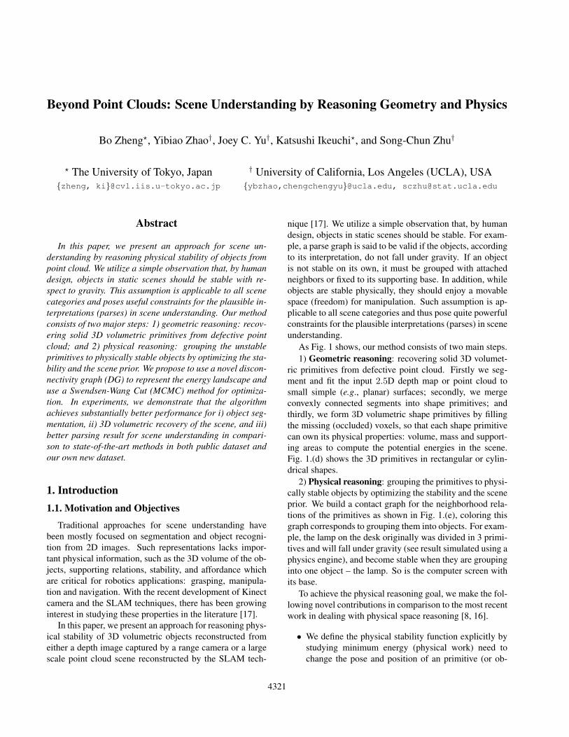
Figure 2. (a) Two 1-degree IAMs f1 and f2 (in blue and red linesrespectively) are fitted to the 3-Layer point cloud. The light redand blue areas denote in which functions f1, f2 and f3 are minus.(b) Invisible space estimation and voxel completion. Four types ofvoxels are estimated: invisible voxels (light green), empty voxels(white), surface voxels (red and blue dots), and the voxels filled inthe invisible space (colored square in light red or blue).

engines in graphics can accurately simulate the motion ofobjects under gravity, but it is computationally expensivefor the purpose of measuring object stability.

2. Geometric reasoning

Given a point cloud of scene, the goal of geometric rea-soning is to infer the object primitives (e.g., the colored ob-jects in Fig. 1 (d)), such as that each primitive can own phys-ical properties (e.g., volume, mass, supporting area, etc.).We infer the object primitives with two major steps: 1) pointcloud segmentation and 2) Volumetric completion.

2.1. Segmentation with implicit algebraic models

We first adopt implicit algebraic models (IAMs) [4] toseparate point cloud into several simple surfaces. We adopta split-and-merge strategy as: 1) splitting the point cloudinto simple and smooth regions by IAM fitting, and then 2)merging the regions which are “convexly” connected eachother. As a 2D example illustrated in Fig. 2.(a), supposethe 2D point cloud is first split into three line segments withfirst-order IAM fitting: f1, f2 and f3, and then f2 and f3are merged together, since they are “convexly” connected.

Splitting point cloud. The objective in this process can beconsidered as to find out the 3D regions, and each of themcan be well fitted by an IAM.

The IAM fitting for each region can be formulated inleast squares optimization using the 3-Layer method pro-posed by Blane et al. [4]. As shown in Figure 2.(a), it firstgenerate two extra point layers: Γ−(green points) and Γ+

(light blue points) along the normals of points in the origi-nal region M (red and blue points). Then an IAM can be fit

toM by linear least-squared method with linear constraints:

f(pi) =

0, pi ∈M+di, pi ∈ Γ+

−di, pi ∈ Γ−

, (1)

where f is an implicit polynomial, ±d is the Euclidean dis-tance how long the two points move along the normals inopposite directions. Therefore, as shown in Fig. 2 (a), eachIAM fit can split the space into two parts: “inside” (coloredwith negative value) and “outside” (uncolored (white) withpositive value).

For splitting point cloud into pieces, we adopt regiongrowing scheme [18]. Our method can be described as:starting from several given seeds, the regions grow untilthere is no unlabeled point can be fitted by certain IAM. Inthis paper, we adopt the IAM of 1 or 2 degree, i.e., planesor second order algebraic surfaces and the IAM fitting algo-rithm proposed by Zheng et al. [22] to select the models ina degree-increasing manner.Merging “convexly” connect regions. The splitting strat-egy seems separating the points to be object faces (e.g., abox can be split into six faces). However we can furthermerge the “convexly” connected regions to better representobject parts (primitives).

To this end, we first define “convex connection” of tworegions as follow:

Definition 1. for any line segment L whose two ends are intwo connected regions with IAM fits fi and fj respectively,if the points on this line, {∀pl|pl ∈ L}, satisfy fi(pl) < 0and fj(pl) < 0, then we say regions i and j are convexlyconnected.

To detect the convex connection, as shown in Fig. 2 (a),we first randomly sample several line points (in dark dotlines) between connected regions, and then check them ifsatisfy the convexly connected relationship defined above.In practice, we merge the convex connections when the fol-lowing condition is satisfied:

#{p|pl ∈ L ∧ fi(pl) < 0 ∧ fj(pl) < 0}#{p|pl ∈ L}

> δ, (2)

where the ratio threshold δ is set as 0.6 according the sensornoise. In Fig 2 (a), since the dark points connecting f2 andf3 are submerged by both minus regions of them.

2.2. Volumetric space completion

To obtain the physical properties for each object prim-itive (e.g., size, mass etc.), we need volumetric represen-tation but not surface segments. Thus, we complete eachsurface segment into a volumetric (voxel-based) primitiveunder three assumptions: a) Occlusion assumption: voxelsoccluded by the observed point cloud could be parts of ob-jects. b) Solid assumption: hollow object is not preferred

4323

(e.g., plane should not with holes, or a box should be solid).c) Manhattan assumption: most object shapes are alignedwith Manhattan axes.Voxel generation and gravity direction We first generatevoxels for each segment obtained by above point cloud seg-mentation by 1) detecting Manhattan axes [7], 2) construct-ing voxels from point cloud along Manhattan axes by octreeconstruction method [19], and 3) detecting gravity direc-tion. To detect gravity direction, we simply choose the onewith smallest angle to the vertical axis of sensor coordinatesystem.Invisible (occluded) space estimation. The space behindthe point clouds and beyond the view angles is not visiblefrom the camera’s perspective. However this invisible spaceis very helpful for completing the missing voxels from oc-clusion. Inspired by Furukawa’s method in [7], the Man-hattan space is carved by the point cloud into three spaces(as shown in Figure 2(b)): Object surface S (colored-dotsvoxels), Invisible space U (light green voxels) and Visiblespace E (white voxels).Voxels filling. We complete an object primitive from eachlabeled surface segment. Suppose each convex surface seg-ment is the visible part of a primitive, we complete invisiblepart by filling voxels in a visual hull which is occluded bythe surface under two assumptions: 1) as lights travel inlines, the voxels complected are behind the point clouds, asshown in Fig. 2.(b); 2) a primitive should be completed if itcan be seen from at least two directions of Manhattan axes.Therefore our algorithm can be simply described as:Loop: for each invisible voxel vi ∈ U, i = 1, 2, . . .

1) From vi, searching the voxels along 6 directions ofManhattan axes, to collect six nearest surface voxels {vj ∈S} (j ≤ 6).

2) Checking the label for each vj , if there exist more thantwo same labels, then assign this label to voxel vi.

3. Modelling object stability3.1. Energy landscapes

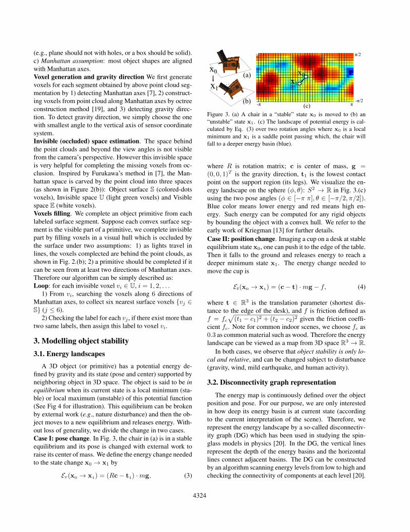
A 3D object (or primitive) has a potential energy de-fined by gravity and its state (pose and center) supported byneighboring object in 3D space. The object is said to be inequilibrium when its current state is a local minimum (sta-ble) or local maximum (unstable) of this potential function(See Fig 4 for illustration). This equilibrium can be brokenby external work (e.g., nature disturbance) and then the ob-ject moves to a new equilibrium and releases energy. With-out loss of generality, we divide the change in two cases.Case I: pose change. In Fig. 3, the chair in (a) is in a stableequilibrium and its pose is changed with external work toraise its center of mass. We define the energy change neededto the state change x0 → x1 by

Er(x → x) = (Rc− t) ·mg, (3)

-π π

π/2

-π/2

x0x1

(a)

(b)(c)

x0

x1

Figure 3. (a) A chair in a “stable” state x0 is moved to (b) an“unstable” state x1. (c) The landscape of potential energy is cal-culated by Eq. (3) over two rotation angles where x0 is a localminimum and x1 is a saddle point passing which, the chair willfall to a deeper energy basin (blue).

where R is rotation matrix; c is center of mass, g =(0, 0, 1)T is the gravity direction, t1 is the lowest contactpoint on the support region (its legs). We visualize the en-ergy landscape on the sphere (φ, θ): S2 → R in Fig. 3.(c)using the two pose angles (φ ∈ [−π π], θ ∈ [−π/2, π/2]).Blue color means lower energy and red means high en-ergy. Such energy can be computed for any rigid objectsby bounding the object with a convex hull. We refer to theearly work of Kriegman [13] for further details.Case II: position change. Imaging a cup on a desk at stableequilibrium state x0, one can push it to the edge of the table.Then it falls to the ground and releases energy to reach adeeper minimum state x1. The energy change needed tomove the cup is

Et(x → x) = (c− t) ·mg − f, (4)

where t ∈ R3 is the translation parameter (shortest dis-tance to the edge of the desk), and f is friction defined asf = fc

√(t1 − c1)2 + (t2 − c2)2 given the friction coeffi-

cient fc. Note for common indoor scenes, we choose fc as0.3 as common material such as wood. Therefore the energylandscape can be viewed as a map from 3D space R3 → R.

In both cases, we observe that object stability is only lo-cal and relative, and can be changed subject to disturbance(gravity, wind, mild earthquake, and human activity).

3.2. Disconnectivity graph representation

The energy map is continuously defined over the objectposition and pose. For our purpose, we are only interestedin how deep its energy basin is at current state (accordingto the current interpretation of the scene). Therefore, werepresent the energy landscape by a so-called disconnectiv-ity graph (DG) which has been used in studying the spin-glass models in physics [20]. In the DG, the vertical linesrepresent the depth of the energy basins and the horizontallines connect adjacent basins. The DG can be constructedby an algorithm scanning energy levels from low to high andchecking the connectivity of components at each level [20].

4324

(a)

(b)

(c)

0 5 10 150

35

70

# iteration

Ene

rgy

rele

ased

(d)

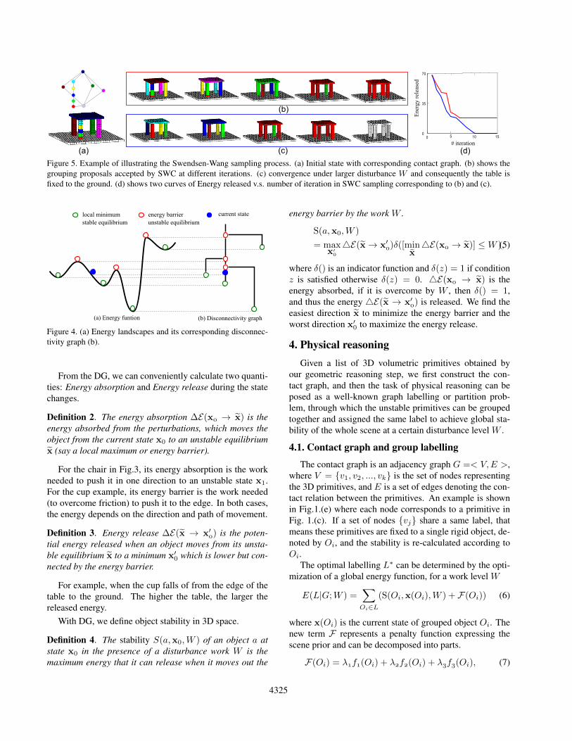
Figure 5. Example of illustrating the Swendsen-Wang sampling process. (a) Initial state with corresponding contact graph. (b) shows thegrouping proposals accepted by SWC at different iterations. (c) convergence under larger disturbance W and consequently the table isfixed to the ground. (d) shows two curves of Energy released v.s. number of iteration in SWC sampling corresponding to (b) and (c).

energy barrierunstable equilibrium

local minimumstable equilibrium

(a) Energy funtion (b) Disconnectivity graph

current state

Figure 4. (a) Energy landscapes and its corresponding disconnec-tivity graph (b).

From the DG, we can conveniently calculate two quanti-ties: Energy absorption and Energy release during the statechanges.

Definition 2. The energy absorption ∆E(x → x) is theenergy absorbed from the perturbations, which moves theobject from the current state x0 to an unstable equilibriumx (say a local maximum or energy barrier).

For the chair in Fig.3, its energy absorption is the workneeded to push it in one direction to an unstable state x1.For the cup example, its energy barrier is the work needed(to overcome friction) to push it to the edge. In both cases,the energy depends on the direction and path of movement.

Definition 3. Energy release ∆E(x → x′) is the poten-tial energy released when an object moves from its unsta-ble equilibrium x to a minimum x′0 which is lower but con-nected by the energy barrier.

For example, when the cup falls of from the edge of thetable to the ground. The higher the table, the larger thereleased energy.

With DG, we define object stability in 3D space.

Definition 4. The stability S(a,x0,W ) of an object a atstate x0 in the presence of a disturbance work W is themaximum energy that it can release when it moves out the

energy barrier by the work W .

S(a,x0,W )

= maxx′

0

4E(x→ x′)δ([minx4E(x → x)] ≤W ),(5)

where δ() is an indicator function and δ(z) = 1 if conditionz is satisfied otherwise δ(z) = 0. 4E(x → x) is theenergy absorbed, if it is overcome by W , then δ() = 1,and thus the energy 4E(x → x′) is released. We find theeasiest direction x to minimize the energy barrier and theworst direction x′0 to maximize the energy release.

4. Physical reasoningGiven a list of 3D volumetric primitives obtained by

our geometric reasoning step, we first construct the con-tact graph, and then the task of physical reasoning can beposed as a well-known graph labelling or partition prob-lem, through which the unstable primitives can be groupedtogether and assigned the same label to achieve global sta-bility of the whole scene at a certain disturbance level W .

4.1. Contact graph and group labelling

The contact graph is an adjacency graph G =< V,E >,where V = {v1, v2, ..., vk} is the set of nodes representingthe 3D primitives, and E is a set of edges denoting the con-tact relation between the primitives. An example is shownin Fig.1.(e) where each node corresponds to a primitive inFig. 1.(c). If a set of nodes {vj} share a same label, thatmeans these primitives are fixed to a single rigid object, de-noted by Oi, and the stability is re-calculated according toOi.

The optimal labelling L∗ can be determined by the opti-mization of a global energy function, for a work level W

E(L|G;W ) =∑Oi∈L

(S(Oi,x(Oi),W ) + F(Oi)) (6)

where x(Oi) is the current state of grouped object Oi. Thenew term F represents a penalty function expressing thescene prior and can be decomposed into parts.

F(Oi) = λf(Oi) + λf(Oi) + λf(Oi), (7)

4325

where f1 is the total number of voxels in objectOi; f2 is thegeometric complexity ofOi, which can be simply computedas the summation of the difference of normals for any twoconnected voxels on its surface; and f3 is designed by thefreedom of object movement on its support area. f3 can becalculated as the ratio between the support plane and thecontact area #S

#CA of each pair of primitives {vj , vk ∈ Oi},where one of them is supported by the other. After they areregularized to the scale of objects, the parameters λ1, λ2 andλ3 are set as 0.1, 0.1, and 0.7 in our experiment. Note, thethird penalty is designed from the observation that, e.g., acup should have freedom of movement supported by a desk,and therefore the penalty arise if the mouse is assigned bysame label to the table.

4.2. Inference of Maximum stability

As the label of primitives are coupled with each other,we adopt the graph partition algorithm Swendsen-Wang Cut(SWC) [2] for efficient MCMC inference. To obtain glob-ally optimal L∗by the SWC, the next 3 main steps worksiteratively until convergence.

(i) Edge turn-on probability. Each edge e ∈ E is as-sociated with a Bernoulli random variable µe ∈ {on, off}indicating whether the edge is turned on or off, and a weightreflecting the possibility of doing so. In this work, for eachedge e =< vi, vj >, we define its turn-on probability as:

qe = p(µe = on|vi, vj) = exp(−(F (vi, vj)/T ), (8)

where T is temperature factor and F (·, ·) denotes the fea-ture between two connected primitives. Here we adopt afeature using the ratio between contact area (plane) and ob-ject planes as: F = #CA

max(#Ai,#Aj), where CA is the con-

tact area, Ai and Aj are the areas of vi and vj on the sameplane of CA.

(ii) Graph Clustering. Given the current label map, itremoves all edges between nodes of different categories.Then all the remaining edges are turned on independentlywith the probability qe. Thus, we have a set of connectedcomponents (CCPs) Π’s, in which all nodes have the samecategory label.

(iii) Graph Flipping. It randomly selects a CCP Πi fromthe set formed in step (ii) with a uniform probability, andthen flips the labels of all nodes in Πi to a category c ∈{1, 2, ..., C}. The flip is accepted with probability [2]:

α(L→ L′) = min (1,Q(L′ → L)E(L′|G;W )

Q(L→ L′)E(L|G;W )). (9)

Fig. 5 illustrates the process of labeling a number ofprimitives of a table into a single object. SWC starts withan initial graph in (a), and some of the sampling proposalsare accepted by the probability (9) shown in (b) and (c), re-sulted the energy v.s. iterations in (d). It is worth noticing

Cut Discrepancy Hamming Hamming−Rm Hamming−Rf0

0.05

0.1

0.15

0.2

0.25

0.3

0.35

0.4

0.45

Err

or

Region growing [18]Geometric ReasoningPhysics reasoning

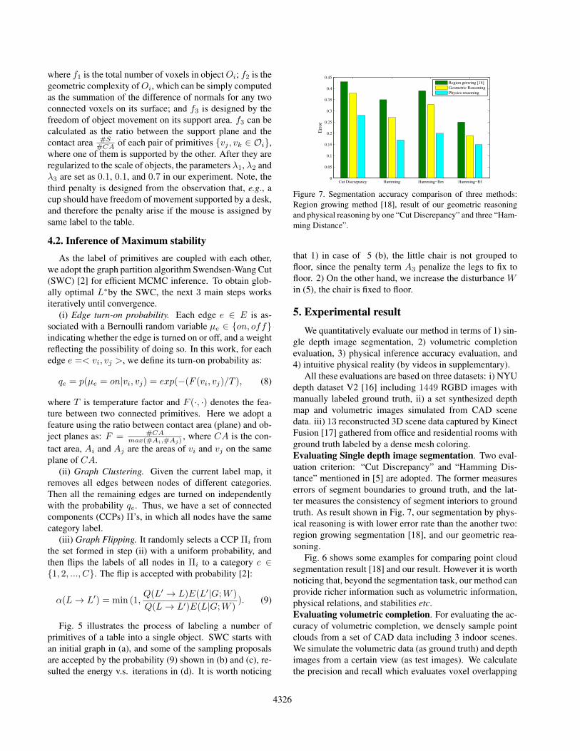
Figure 7. Segmentation accuracy comparison of three methods:Region growing method [18], result of our geometric reasoningand physical reasoning by one “Cut Discrepancy” and three “Ham-ming Distance”.

that 1) in case of 5 (b), the little chair is not grouped tofloor, since the penalty term A3 penalize the legs to fix tofloor. 2) On the other hand, we increase the disturbance Win (5), the chair is fixed to floor.

5. Experimental resultWe quantitatively evaluate our method in terms of 1) sin-

gle depth image segmentation, 2) volumetric completionevaluation, 3) physical inference accuracy evaluation, and4) intuitive physical reality (by videos in supplementary).

All these evaluations are based on three datasets: i) NYUdepth dataset V2 [16] including 1449 RGBD images withmanually labeled ground truth, ii) a set synthesized depthmap and volumetric images simulated from CAD scenedata. iii) 13 reconstructed 3D scene data captured by KinectFusion [17] gathered from office and residential rooms withground truth labeled by a dense mesh coloring.Evaluating Single depth image segmentation. Two eval-uation criterion: “Cut Discrepancy” and “Hamming Dis-tance” mentioned in [5] are adopted. The former measureserrors of segment boundaries to ground truth, and the lat-ter measures the consistency of segment interiors to groundtruth. As result shown in Fig. 7, our segmentation by phys-ical reasoning is with lower error rate than the another two:region growing segmentation [18], and our geometric rea-soning.

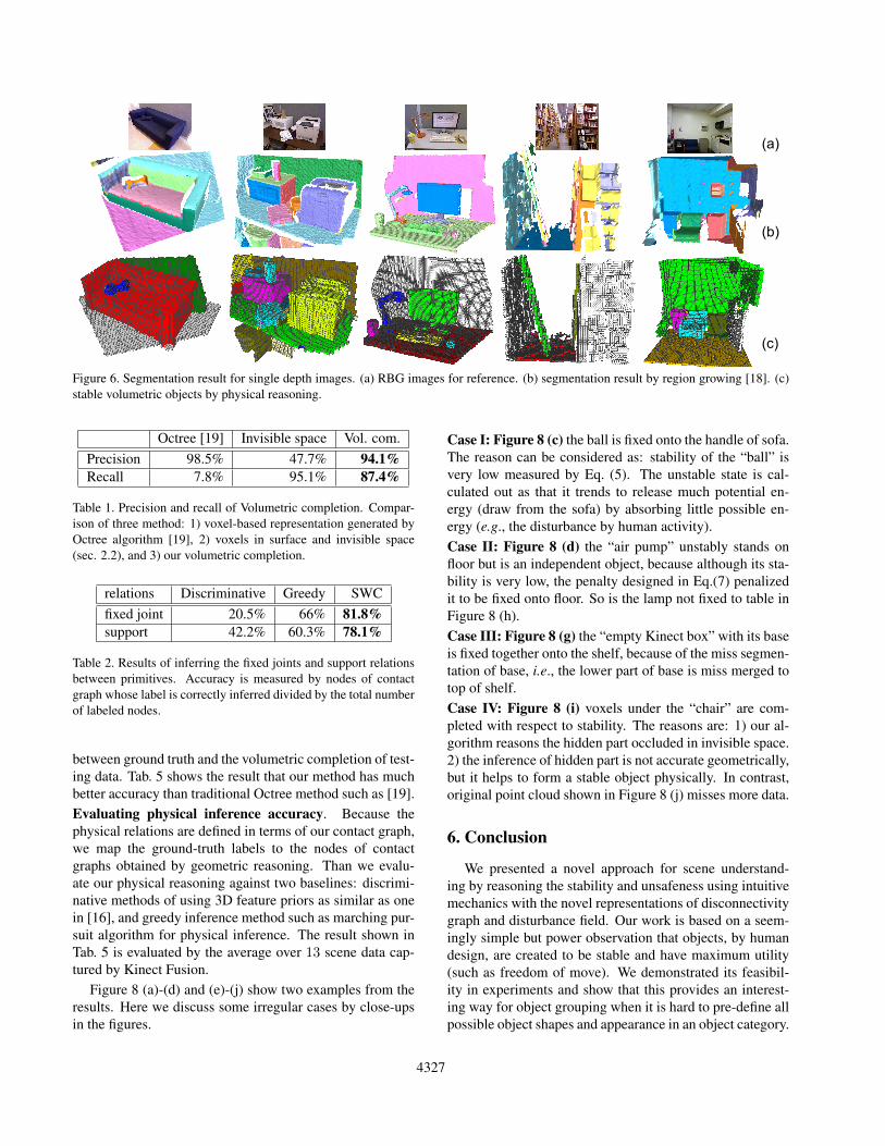
Fig. 6 shows some examples for comparing point cloudsegmentation result [18] and our result. However it is worthnoticing that, beyond the segmentation task, our method canprovide richer information such as volumetric information,physical relations, and stabilities etc.Evaluating volumetric completion. For evaluating the ac-curacy of volumetric completion, we densely sample pointclouds from a set of CAD data including 3 indoor scenes.We simulate the volumetric data (as ground truth) and depthimages from a certain view (as test images). We calculatethe precision and recall which evaluates voxel overlapping

4326

(a)

(b)

(c)

Figure 6. Segmentation result for single depth images. (a) RBG images for reference. (b) segmentation result by region growing [18]. (c)stable volumetric objects by physical reasoning.

Octree [19] Invisible space Vol. com.Precision 98.5% 47.7% 94.1%Recall 7.8% 95.1% 87.4%

Table 1. Precision and recall of Volumetric completion. Compar-ison of three method: 1) voxel-based representation generated byOctree algorithm [19], 2) voxels in surface and invisible space(sec. 2.2), and 3) our volumetric completion.

relations Discriminative Greedy SWCfixed joint 20.5% 66% 81.8%support 42.2% 60.3% 78.1%

Table 2. Results of inferring the fixed joints and support relationsbetween primitives. Accuracy is measured by nodes of contactgraph whose label is correctly inferred divided by the total numberof labeled nodes.

between ground truth and the volumetric completion of test-ing data. Tab. 5 shows the result that our method has muchbetter accuracy than traditional Octree method such as [19].Evaluating physical inference accuracy. Because thephysical relations are defined in terms of our contact graph,we map the ground-truth labels to the nodes of contactgraphs obtained by geometric reasoning. Than we evalu-ate our physical reasoning against two baselines: discrimi-native methods of using 3D feature priors as similar as onein [16], and greedy inference method such as marching pur-suit algorithm for physical inference. The result shown inTab. 5 is evaluated by the average over 13 scene data cap-tured by Kinect Fusion.

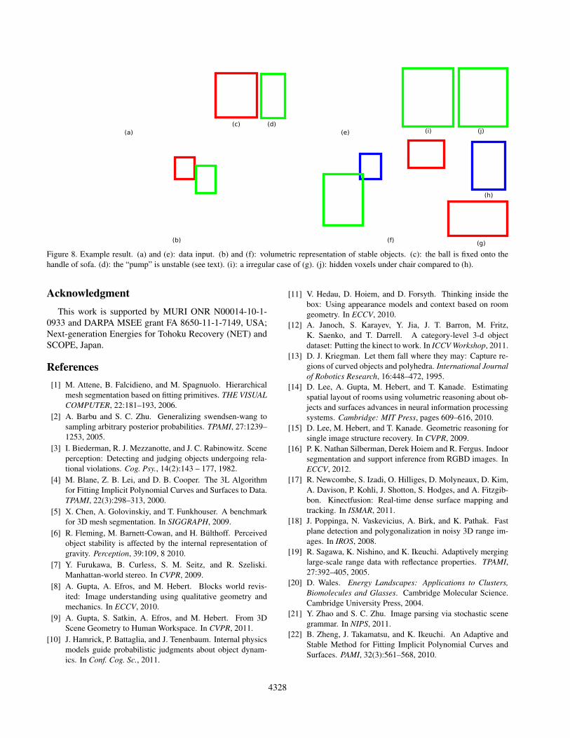
Figure 8 (a)-(d) and (e)-(j) show two examples from theresults. Here we discuss some irregular cases by close-upsin the figures.

Case I: Figure 8 (c) the ball is fixed onto the handle of sofa.The reason can be considered as: stability of the “ball” isvery low measured by Eq. (5). The unstable state is cal-culated out as that it trends to release much potential en-ergy (draw from the sofa) by absorbing little possible en-ergy (e.g., the disturbance by human activity).Case II: Figure 8 (d) the “air pump” unstably stands onfloor but is an independent object, because although its sta-bility is very low, the penalty designed in Eq.(7) penalizedit to be fixed onto floor. So is the lamp not fixed to table inFigure 8 (h).Case III: Figure 8 (g) the “empty Kinect box” with its baseis fixed together onto the shelf, because of the miss segmen-tation of base, i.e., the lower part of base is miss merged totop of shelf.Case IV: Figure 8 (i) voxels under the “chair” are com-pleted with respect to stability. The reasons are: 1) our al-gorithm reasons the hidden part occluded in invisible space.2) the inference of hidden part is not accurate geometrically,but it helps to form a stable object physically. In contrast,original point cloud shown in Figure 8 (j) misses more data.

6. Conclusion

We presented a novel approach for scene understand-ing by reasoning the stability and unsafeness using intuitivemechanics with the novel representations of disconnectivitygraph and disturbance field. Our work is based on a seem-ingly simple but power observation that objects, by humandesign, are created to be stable and have maximum utility(such as freedom of move). We demonstrated its feasibil-ity in experiments and show that this provides an interest-ing way for object grouping when it is hard to pre-define allpossible object shapes and appearance in an object category.

4327

(b)

(a)

(h)

(f) (g)

(d)(c)(i) (j)(e)

Figure 8. Example result. (a) and (e): data input. (b) and (f): volumetric representation of stable objects. (c): the ball is fixed onto thehandle of sofa. (d): the “pump” is unstable (see text). (i): a irregular case of (g). (j): hidden voxels under chair compared to (h).

AcknowledgmentThis work is supported by MURI ONR N00014-10-1-

0933 and DARPA MSEE grant FA 8650-11-1-7149, USA;Next-generation Energies for Tohoku Recovery (NET) andSCOPE, Japan.

References[1] M. Attene, B. Falcidieno, and M. Spagnuolo. Hierarchical

mesh segmentation based on fitting primitives. THE VISUALCOMPUTER, 22:181–193, 2006.

[2] A. Barbu and S. C. Zhu. Generalizing swendsen-wang tosampling arbitrary posterior probabilities. TPAMI, 27:1239–1253, 2005.

[3] I. Biederman, R. J. Mezzanotte, and J. C. Rabinowitz. Sceneperception: Detecting and judging objects undergoing rela-tional violations. Cog. Psy., 14(2):143 – 177, 1982.

[4] M. Blane, Z. B. Lei, and D. B. Cooper. The 3L Algorithmfor Fitting Implicit Polynomial Curves and Surfaces to Data.TPAMI, 22(3):298–313, 2000.

[5] X. Chen, A. Golovinskiy, and T. Funkhouser. A benchmarkfor 3D mesh segmentation. In SIGGRAPH, 2009.

[6] R. Fleming, M. Barnett-Cowan, and H. Bulthoff. Perceivedobject stability is affected by the internal representation ofgravity. Perception, 39:109, 8 2010.

[7] Y. Furukawa, B. Curless, S. M. Seitz, and R. Szeliski.Manhattan-world stereo. In CVPR, 2009.

[8] A. Gupta, A. Efros, and M. Hebert. Blocks world revis-ited: Image understanding using qualitative geometry andmechanics. In ECCV, 2010.

[9] A. Gupta, S. Satkin, A. Efros, and M. Hebert. From 3DScene Geometry to Human Workspace. In CVPR, 2011.

[10] J. Hamrick, P. Battaglia, and J. Tenenbaum. Internal physicsmodels guide probabilistic judgments about object dynam-ics. In Conf. Cog. Sc., 2011.

[11] V. Hedau, D. Hoiem, and D. Forsyth. Thinking inside thebox: Using appearance models and context based on roomgeometry. In ECCV, 2010.

[12] A. Janoch, S. Karayev, Y. Jia, J. T. Barron, M. Fritz,K. Saenko, and T. Darrell. A category-level 3-d objectdataset: Putting the kinect to work. In ICCV Workshop, 2011.

[13] D. J. Kriegman. Let them fall where they may: Capture re-gions of curved objects and polyhedra. International Journalof Robotics Research, 16:448–472, 1995.

[14] D. Lee, A. Gupta, M. Hebert, and T. Kanade. Estimatingspatial layout of rooms using volumetric reasoning about ob-jects and surfaces advances in neural information processingsystems. Cambridge: MIT Press, pages 609–616, 2010.

[15] D. Lee, M. Hebert, and T. Kanade. Geometric reasoning forsingle image structure recovery. In CVPR, 2009.

[16] P. K. Nathan Silberman, Derek Hoiem and R. Fergus. Indoorsegmentation and support inference from RGBD images. InECCV, 2012.

[17] R. Newcombe, S. Izadi, O. Hilliges, D. Molyneaux, D. Kim,A. Davison, P. Kohli, J. Shotton, S. Hodges, and A. Fitzgib-bon. Kinectfusion: Real-time dense surface mapping andtracking. In ISMAR, 2011.

[18] J. Poppinga, N. Vaskevicius, A. Birk, and K. Pathak. Fastplane detection and polygonalization in noisy 3D range im-ages. In IROS, 2008.

[19] R. Sagawa, K. Nishino, and K. Ikeuchi. Adaptively merginglarge-scale range data with reflectance properties. TPAMI,27:392–405, 2005.

[20] D. Wales. Energy Landscapes: Applications to Clusters,Biomolecules and Glasses. Cambridge Molecular Science.Cambridge University Press, 2004.

[21] Y. Zhao and S. C. Zhu. Image parsing via stochastic scenegrammar. In NIPS, 2011.

[22] B. Zheng, J. Takamatsu, and K. Ikeuchi. An Adaptive andStable Method for Fitting Implicit Polynomial Curves andSurfaces. PAMI, 32(3):561–568, 2010.

4328