Embed Size (px)
Citation preview

Dis cus si on Paper No. 16-068
Beyond Equal Rights: Equality of Opportunity in
Political Participation Paul Hufe and Andreas Peichl
Dis cus si on Paper No. 16-068
Beyond Equal Rights: Equality of Opportunity in
Political Participation Paul Hufe and Andreas Peichl
Download this ZEW Discussion Paper from our ftp server:
http://ftp.zew.de/pub/zew-docs/dp/dp16068.pdf
Die Dis cus si on Pape rs die nen einer mög lichst schnel len Ver brei tung von neue ren For schungs arbei ten des ZEW. Die Bei trä ge lie gen in allei ni ger Ver ant wor tung
der Auto ren und stel len nicht not wen di ger wei se die Mei nung des ZEW dar.
Dis cus si on Papers are inten ded to make results of ZEW research prompt ly avai la ble to other eco no mists in order to encou ra ge dis cus si on and sug gesti ons for revi si ons. The aut hors are sole ly
respon si ble for the con tents which do not neces sa ri ly repre sent the opi ni on of the ZEW.
Beyond Equal Rights: Equality of Opportunity in Political
Participation∗
Paul Hufe Andreas Peichl
Preliminary Version: 10.10.2016.
Abstract
It is well understood that political participation is stratied by socio-economic
characteristics. Yet it is an open question how this nding bears on the normative
evaluation of the democratic process. In this paper we argue that the equality of op-
portunity (EOp) concept furnishes an attractive framework to answer this question.
Drawing on the analytical tools developed by an expanding empirical literature on EOp
we investigate to what extent political participation is determined by factors that lie
beyond individual control (circumstances) and thus is unfairly distributed. Using rich
panel data from the US, we nd that a lack of political opportunity is particularly
pronounced for contacts with ocials, participation in rallies and marches, and mem-
bership in political organizations. These opportunity shortages tend to complement
each other across activities and persist over time. While family characteristics and
psychological dispositions during childhood emanate as the strongest determinants,
genetic variation is a small yet signicant contributor to unequal political opportuni-
ties in the US.
JEL-Codes: D39; D63; D72
Keywords: Equality of Opportunity; Political Participation; Genes
∗Hufe: ZEW Mannheim and University of Mannheim ([email protected]); Peichl (corresponding author):
ZEWMannheim, University of Mannheim, IZA and CESifo. Postal Address: ZEWMannheim, L7,1, 68161
Mannheim, Germany ([email protected]). This paper has beneted from discussions with Alain Trannoy and
Daniel Hopp. We are also grateful to audiences at SMYE Lisbon, LAGV Aix-en-Provence, Canazei Winter
School, SSSI Bonn and seminar participants in Mannheim for many useful comments and suggestions. This
research uses data from Add Health, a program project directed by Kathleen Mullan Harris and designed
by J. Richard Udry, Peter S. Bearman, and Kathleen Mullan Harris at the University of North Carolina
at Chapel Hill, and funded by grant P01-HD31921 from the Eunice Kennedy Shriver National Institute
of Child Health and Human Development, with cooperative funding from 23 other federal agencies and
foundations. Special acknowledgment is due Ronald R. Rindfuss and Barbara Entwisle for assistance in
the original design. Information on how to obtain the Add Health data les is available on the Add Health
website (http://www.cpc.unc.edu/addhealth). No direct support was received from grant P01-HD31921
for this analysis.
1 Introduction
Rousseau (1978) supposed that in well-run states everyone rushes to the assemblies.
Judging by that standard Western democracies are in increasingly bad shape as the drop
in voter participation is a shared tendency in these countries (OECD, 2015). The lack
in political participation and the underlying stratication has been researched extensively
by scholars of political sociology, who nd that participation varies positively with socio-
economic status (SES). The SES framework purports that people with lower socio-economic
status, as embodied in income and education, dispose of fewer resources to cover the cost
of political participation. The importance of SES varies across political activities due to
the dierent nature and amounts of the inputs required (Bénabou, 2000). For instance,
formulating a petition to a local representative arguably requires a more comprehensive
skill-set than joining a protest march. Campaign contributions require nancial leeway
and are highly skewed in favor of the upper percentiles of the income distribution. In
general, however, the link between education, nancial capacity and political participation,
as emanating from research in political sociology is stable and likewise accepted among
scholars of economics (Bourguignon and Verdier, 2000; Campante, 2011; Milligan et al.,
2004).
In spite of the breadth of research undertaken to discern the determinants of political
participation, one is tempted to ask how these ndings bear on the normative evaluation of
democratic outcomes. Verba et al. (1993) suggest that a verdict on the legitimacy of demo-
cratic outcomes depends on the extent to which political inactivity is self-inicted instead
of being attributable to factors beyond individual control. In later writings these authors
formulate this requirement more explicitly by highlighting the importance of equity in the
conditions or opportunities aorded to a player [in the political game] (Verba, 2006). Yet
in spite of the wide appreciation of the normative importance of political opportunities,
no rigorous empirical investigation has been forthcoming to this date (Brady et al., 2015).
In this paper we estimate equality of opportunity (EOp, or IOp for inequality of op-
portunity) in political participation in the United States. To be sure, we are interested
in eective opportunities as opposed to merely formal opportunities. In the US the right
to vote is unrestricted as is the right to free speech and association. What we address
in this work is the extent to which dierences in the capacity to negotiate these formal
opportunities are due to factors beyond individual control. We focus on the following
seven forms of participation: (i) vote registration for the 2000 Presidential election, (ii)
vote casting in the 2000 Presidential election, (iii) contact to ocials, (iv) participation
in rallies or marches, (v) membership in political organizations, (vi) volunteering in civic
organizations, and lastly (vii) the vote frequency in statewide and local elections. Thereby
we speak to two distinct branches of existing literature.
First, we widen the scope of the existing (economic) literature on EOp by considering
a new outcome dimension, namely political participation. Research to date has focused
1
on income (Björklund et al., 2012; Ferreira and Gignoux, 2011; Pistolesi, 2009), education
(Brunori et al., 2012) or health outcomes (Fleurbaey and Schokkaert, 2009; Rosa Dias,
2009). Furthermore, to the best of our knowledge this is the rst work that expands the
set of circumstance variables by genotype information. By virtue of the fact that genes
are xed, they represent the purest measure of biological inheritance (Fowler et al., 2008)
and thus should be of particular interest in the estimation of EOp.
Second, the determinants of political participation are vastly researched in the eld of
political sociology (for comprehensive overviews: Barrett and Brunton-Smith, 2014; Verba
et al., 2012). In addition to indicators of SES the literature has considered a host of dierent
variables that are of interest from an equal-opportunity perspective. One group of works
has focused on immutable personal characteristics such as race (Verba et al., 1993), sex
(Schlozman et al., 1995), age and cohort (Blais et al., 2004). Another group has considered
inuence factors that are not strictly immutable but play out before the age of consent,
such as parental political participation (Niemi and Jennings, M. Kent, 1991; Plutzer, 2002),
local networks in the area of upbringing (Gimpel et al., 2006), or voluntary participation in
youth organizations (McFarland and Thomas, 2006). All these factors have been analyzed
in their own right but have not been used to construct a comprehensive measure of IOp
a gap that will be addressed in this paper.
Our results suggest signicant IOp along each considered dimension of political partici-
pation, especially with respect to contacts to ocials, participation in rallies and marches,
and the membership in political organizations. In all of the aforementioned dimensions
we calculate type-specic dissimilarity indexes of more than 50%. It is noteworthy that
opportunity disadvantages do not set-o each other across dierent dimensions. Disadvan-
tages in either activity are positively correlated with opportunity disadvantages in other
forms of political participation. Furthermore, our results suggest that opportunity disad-
vantages persist over time. Family circumstances and psychological dispositions as a child
consistently exert the strongest inuence on unequal opportunities across all forms of po-
litical participation. We nd a statistically signicant inuence of genetic information on
IOp, which however is small in magnitude in comparison with the previously mentioned
circumstance groups.
In the following section we outline the conceptual framework as well as the associated
estimation strategy. In section 3 we describe the data set, followed by the presentation of
the results in section 4. Lastly, we conclude with section 5.
2 Conceptual Framework
EOp is a framework for the normative assessment of the distribution of some desirable
outcome p, such as health status, education or income. It is rooted in a philosophical
discourse on the principles of distributive justice. The underlying normative cut that
people should be held responsible for their choices only, not for factors beyond their con-
2
trol resonates in the most prominent contributions to this branch of the philosophical
discourse (Arneson, 1989; Cohen, 1989; Dworkin, 1981; Rawls, 1971; Sen, 1979). On the
one hand, the normative principle implies that inequality is unacceptable if it is rooted
beyond the sphere of individual control. It is the task of social policy to correct the out-
come distribution, for instance by means of transfer payments in the case of income. On
the other hand, equality of outcomes is not a demand of justice as long as we reject the
idea that the human endeavor is perfectly deterministic. To the extent that inequality is
a result of individual eort, proponents of EOp accept the outcome distribution as fair.
The formalization of the EOp principles by Roemer (1998) has stimulated an extensive
body of literature in the eld of economics (see Ferreira and Peragine, 2015; Roemer
and Trannoy, 2015, for recent overviews). Particularly the normative and econometric
properties of dierent measurement approaches have been an area of in-depth interest
(Van de gaer and Ramos, 2016).
The Normative Status of Political Participation It is beyond the ambit of this work
to put forward a comprehensive account of the normative status of political participation.
Yet we want to sketch why political participation is a desirable outcome that warrants the
quest for equal opportunity.
Rousseau (1978) considers three attributes that make political participation inherently
desirable (for a discussion see Pateman, 1970, ch.2). First, it fosters civic education in
the sense that a political act always involves some strategic reasoning that requires the
actor to put herself in the shoes of her fellow citizens. Second, political participation
entails freedom understood as being one's own master. Exercising one's say in the process
of elaborating policies, the laws to which one is subjected are self-prescribed rather than
externally imposed. Lastly, according to Rousseau political participation fosters a sense of
belonging within a community. These notions indicate some inherent value in the act of
participation as such.
Moreover, by means of participating in the political process the constituents of a ju-
risdiction can inuence policies, the consequences of which are fed back to themselves.
Thus political participation also has an instrumental function in protecting the citizen's
(private) interests. An illustrative example is furnished by the debate on why the seminal
Meltzer and Richard (1981) model for redistribution fails to garner empirical support. One
prime contender among other explanations is the assertion that the distribution of political
inuence is biased in the direction of the income distribution (among others Karabarbou-
nis, 2011). That alone would be unproblematic if the preferences of the participating
population were entirely congruent with the abstaining fraction. However this assumption
seems to be contradicted by the nding that [i]n particular, women, youth and African-
Americans appear to have stronger preferences for redistribution (Alesina and Giuliano,
2011). Henceforth, if political activity was stratied by these circumstance characteris-
tics, the participation bias would re-enforce existing inequalities by discounting the call for
3
increased redistribution.
Analytical Approach In line with the underlying normative principle, we decompose
the observed outcome distribution F (p) into a fair and an unfair component. From an
EOp perspective, F (p) would be fair if it was entirely determined by factors that lie within
the realm of control of individuals i. To operationalize this idea, the empirical literature
draws on the concepts of circumstances and eorts the underlying assumption being that
a set of circumstances Ω and a set of eorts Θ jointly determine the outcome of interest p.
Standard examples of circumstances are the biological sex, skin color or the educational
achievement of parents. Examples of eort in the context of political participation are
common indicators for socio-economic status such as educational achievement and income,
or individual behaviors that are targeted towards information gathering, such as news
consumption. The relation between these components can be described by a function
g : Θ× Ω 7→ R+.
It is reasonable to assume that the distribution of eorts is not orthogonal to circum-
stances. For example, on the one hand the gender wage gap is the result of discriminatory
processes in the labor market. On the other hand, it has been shown that females have
increased their labor supply in response to a shrinking gender wage gap (Mulligan and Ru-
binstein, 2008). To phrase it in the terms of EOp: females adjusted their eort in response
to reduced discrimination based on the circumstance variable gender. To the extent that
we want to correct for eorts that are endogenous to circumstances, the relation of interest
can be expressed in the following reduced form:
p = g(Ω,Θ(Ω), ε), (1)
where circumstances Ω and endogenous eort Θ(Ω) are considered as root-causes of unfair
inequality, whereas dierential eort net of circumstance inuence ε yields the fair share
of inequality.
To operationalize this idea econometrically we rely on a method of measurement which
the literature refers to as the ex-ante approach.1 Based on the number of realizations xj
of each circumstance Cj ∈ Ω we can partition the population into a set of types T , where
the number of types is given by K =∏Jj=1 xj . Assume that there were only two relevant
circumstance variables, say biological sex (C1=Male; Female) and family background
(C2=Rich; Poor) with two realizations each. Since x1 = x2 = 2 we can decompose the
population into K = 4 types (Table 1).
Perfect EOp would prevail if all types T k ∈ T faced the same opportunity set and
the observed variation in outcomes was a pure result of dierential eort. As we can
only observe realized individual choices instead of the underlying opportunity space, we
use the type-specic mean realization of the outcome of interest µk(p) as an estimator of
1It is ex-ante in the sense that the need for compensation is determined without regard to the realizationof individual eort. See Van de gaer and Ramos (2016) for more details.
4
Table 1: Example of Type Set
Male Female
Rich Type 1 Type 2Poor Type 3 Type 4
the respective opportunity set. Drawing on the previous type decomposition, we would
conclude that Type 1 faced a larger opportunity set for voting than Type 2, if the average
turnout of the former group exceeded the average turnout of the latter.
Following this logic, we t a logit model with circumstances Cji as the only right-hand
side variables. Note that we use a logit model in our main specications as activities of
political participation are measured in binary variables (see section 3):2
ln( pi
1− pi
)=
J∑j=1
βjCji . (2)
Recall that the observed outcome pi is determined by the function g(Ωi,Θi(Ωi), εi), where
εi represents residual eort net of circumstance inuence. Then, by calculating predicted
probabilities based on equation 2, we eectively sterilize the outcome distribution from the
fair inequality component ε. This yields the estimator for the type-specic opportunity set
µk(p), since Cji = Cjh ∀ i, h ∈ Tk:
µk(p) =exp(
∑Jj=1 βjC
ji )
1 + exp(∑J
j=1 βjCji ). (3)
The resulting distribution of µk(p) is called smoothed distribution, here denoted as Φ.
Note that any inequality in Φ exclusively relates to dierences in circumstances and thus
conicts with the ethics of EOp: the higher the dispersion in Φ, the more variation in F (p)
is explained by circumstances, the higher IOp in political participation.
Equations (2) and (3) illustrate that this procedure yields a lower bound of IOp in
political participation. Variation explained by circumstance variables that are not included
in the estimation, is captured in the error term ε and therefore attributed to the fair share
of inequality. Thus, expanding the circumstance set under consideration always increases
the variation in the smoothed distribution Φ unless these circumstances are orthogonal
to the outcome of interest (see Ferreira and Gignoux, 2011; Niehues and Peichl, 2014,
for thorough discussions). As it is very unlikely that any data set captures all relevant
circumstance variables, the outlined estimator of IOp cannot exceed its true value.
To obtain a scalar measure of IOp we subject Φ to two inequality metrics. First, we
calculate the Gini index which is a default measure in many works on inequality. Second,
we construct a dissimilarity index which is applied in various works on EOp with discrete
2The results are robust towards using logit, probit or linear probability estimations. See section 4.
5
outcomes (Foguel and Veloso, 2014; Paes de Barros et al., 2008). The dissimilarity index,
based on which we will present most of our results, is constructed as follows. In a rst step
we calculate the dispersion in opportunities:
T =1
2N
∑i
∣∣∣µk(p)− 1
N
∑i
µki (p)∣∣∣. (4)
The term within the absolute value brackets indicates by how much a type-specic advan-
tage level diverges from the average realization within the sample. Note that the second
term within the brackets corresponds to the mean of both F (p) and Φ as the error terms in
a logit estimation sum up to zero. The division by two is for interpretive purposes. As the
sum of positive divergences from the average cancels with sum of negative divergences, T
can now be interpreted as the number of opportunities that would have to be redistributed
in order to obtain the fair outcome. In a second step we scale the dispersion measure by
the average realization within the sample to obtain the dissimilarity index:
D =T
1N
∑i µ
ki (p)
=T
µ(5)
We can interpret D as the share of opportunities that is unfairly distributed.
3 Data
The data set for this research endeavor needs to satisfy two conditions. First, given the
lower bound nature of the IOp estimator it needs to provide a large set of circumstance
variables in order to cushion the downward bias of our results. Second, it needs to include
indicator variables for political participation.3 The one study that strikes a balance be-
tween both requirements is the National Longitudinal Study of Adolescent to Adult Health
(Add Health). Add Health is a four-wave panel study that focuses on health-related be-
haviors and the causes of health outcomes. Initial information was collected in 1994/95
on adolescents in grades 7-12 (N = 20, 745) drawing on a stratied sample of 80 High
Schools in the US. In addition to in-depth interviews with adolescents, questionnaires were
administered to school representatives, parents and roughly 90,000 students of the sampled
schools. Importantly, the survey data is linked to additional contextual data from other
data sources such as the Census of Population and Housing, the School District Databook
or the Statistics of the US Bureau of the State Government Finances. In the two most re-
cent waves all respondents observed in Wave 1 (N = 15, 170 and N = 15, 701, respectively)
had achieved the age of consent, which makes it feasible to extract outcome variables on
dierent political activities, such as vote casting.
3In the US context surveys with an explicit focus on political behavior, such as the American National
Election Study (ANES) perform poorly with respect to the rst requirement. The reverse holds true forlongitudinal studies which allow the construction of nely grained type partitions, such as the National
Longitudinal Study of Youth (NLSY79) and the Panel Study of Income Dynamics (PSID).
6
Before proceeding with a description of the variables of interest, we want to give an ac-
count of our understanding of political participation for the purpose of this work. Barrett
and Brunton-Smith (2014) describe political participation as including all activities inu-
encing the development and implementation of public policy and the selection of represen-
tatives entrusted with this process. According to this view participation can be contrasted
to engagement to the extent that the former refers to activities rather than to psychological
dispositions, attitudes and interests. Thus, self-identied interest in politics or ideologi-
cal leanings are beyond the realm of participation. Moreover, political participation can
be contrasted to civic participation, where the latter relates to voluntary activity to the
benet of fellow human beings or the public good. Thus, community services, donations
to and fundraising activities for charities are beyond the realm of the political. In practice,
however, there is a ne line between civic and political participation as evidenced by the
fact that non-political organizations, such as religious communities, often serve as recruit-
ment vehicles for political action (Verba et al., 1993). This leads us to abstract from this
second division.
According to this delineation Add Health provides information on the following forms
of political participation: (i) vote registration for the 2000 Presidential election, (ii) vote
casting in the 2000 Presidential election, (iii) contact to ocials, (iv) participation in rallies
or marches, (v) membership in political organizations (vi), volunteering in civic organiza-
tions, and lastly (vii) the vote frequency in statewide and local elections. Information
on activities (i)-(vi) is sourced from Wave 3 (respondent age: 18-26) and captured in bi-
nary variables indicating whether the respective activity was undertaken within the last
12 months. Information on activity (vii) is sourced from Wave 4 (respondent age: 24-32)
and captured in a self-reported, ordinal variable with four expressions, ranging from al-
ways and often to sometimes and never. For the purpose of this work we decompose
this variable into two binary variables indicating whether people consider themselves to
be always-voter or never-voter. In addition we estimate IOp in income acquisition in
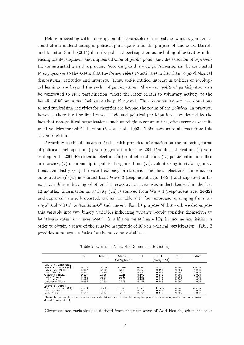
order to obtain a sense of the relative magnitude of IOp in political participation. Table 2
provides summary statistics for the outcome variables.
Table 2: Outcome Variables (Summary Statistics)
N Mean Mean(Weighted)
SD SD(Weighted)
Min Max
Wave 3 (2001/02)Personal Income (k$) 13273 13.597 13.394 16.367 15.477 0.000 500.909Registered (2000) 14087 0.719 0.710 0.450 0.454 0.000 1.000Vote (2000) 13991 0.439 0.419 0.496 0.493 0.000 1.000Contact Ocial 14129 0.026 0.028 0.160 0.164 0.000 1.000Rally/March 14129 0.034 0.032 0.182 0.177 0.000 1.000Political Org. 14099 0.022 0.021 0.147 0.142 0.000 1.000Volunteer Work 14099 0.285 0.279 0.451 0.449 0.000 1.000
Wave 4 (2008)Personal Income (k$) 14314 34.745 34.146 44.826 43.988 0.000 999.995Vote Always 14549 0.247 0.232 0.431 0.422 0.000 1.000Vote Never 14549 0.325 0.348 0.468 0.476 0.000 1.000
Note: In the weighted columns summary statistics are corrected for sampling procedure and sample attrition until Wave3 and 4, respectively.
Circumstance variables are derived from the rst wave of Add Health, when the vast
7
majority of respondents was younger than 18 years of age. We exclude all respondents older
than 17 in the rst wave.4 This restriction is not innocuous. All applied researchers on EOp
need to decide which individual characteristics they are willing to treat as circumstances.
For the purpose of this work we treat the entire child biography up to the age of 18 as a
circumstance and thus do not hold children responsible for any of their prior choices.5
The circumstances we consider are grouped in m = 11 categories, i.e. Ω =∑
m Ωm.
The rst set includes demographic information such as age, migration status and race.
Second, we consider family background information, for instance the education of parents,
the number of siblings and the self-perceived quality of the child-parent relationship. Third,
we take account of variables that are indicative for the quality of the respondent's social
life as a child. Fourth, the childhood neighborhood is evaluated among others in terms
of its safeness and a host of dierent demographic and socio-economic indicators. The
fth set captures characteristics of the school the respondent went to. Among others we
take account of the average class size and the educational achievement of teachers. Sixth,
the ability of respondents is evaluated in terms of the standardized Picture Vocabulary
Test Score (PVT) and whether the respondent skipped or repeated any grades. Aspects
of religiosity captured in the seventh group are represented by the parent's frequency
of attending service and the self-rated importance of religion. Eighth, the respondent's
physical condition during childhood is evaluated along various dimensions ranging from
physical restrictions due to disabilities, over ratings of attractiveness, to a measure for
the Body Mass Index (BMI). Ninth, we integrate a battery of questions on psychological
dispositions such as suicidal intentions, self-ratings of intelligence and expectations for
one's later life. In group ten we take account of risk behaviors including drug and alcohol
abuse of both the respondent and her friends during childhood. Lastly, we include a
battery of binary indicators for the respondent's genetic endowment. The evolving interest
in genes as mediators of environmental inuences that determine political participation
is a noteworthy recent development in the political science literature (Alford et al., 2005;
Benjamin et al., 2012; Fowler et al., 2008; Fowler and Dawes, 2008). The genetic data used
in this work was sourced in the fourth wave of Add Health for a sample of approximately
15,000 respondents.6 In view of the breadth of circumstances considered, a thorough
description of each circumstance variable cannot be given here. The interested reader is
relegated to Table 10 in the Appendix, where summary statistics on all circumstances are
disclosed.
The analysis is conducted using the provided set of sampling weights in order to cor-
rect for the sampling procedure and sample attrition across waves. Hence our analysis is
nationally representative for adolescents enrolled in grades 7-12 in 1994/95.
4Due to this restriction, the age range in our sample decreases from 18-26 (24-32) to 18-24 (24-30) forWave 3 (Wave 4) outcome variables.
5In principle it is possible to specify the responsibility cut-o at an earlier age, say 12 or 16, whichwould restrict the eligible set of circumstances Ω. See Hufe et al. (2015) for a discussion.
6For a more detailed discussion of the genetic variables see section 4.3.
8
4 Results
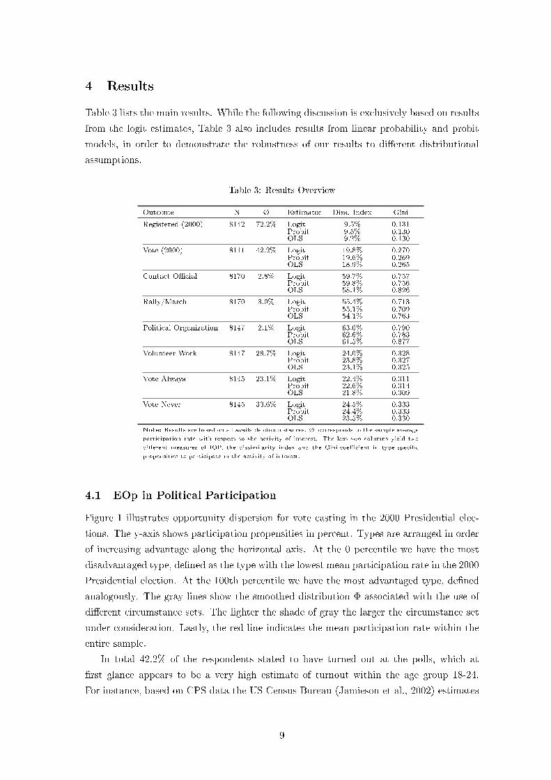
Table 3 lists the main results. While the following discussion is exclusively based on results
from the logit estimates, Table 3 also includes results from linear probability and probit
models, in order to demonstrate the robustness of our results to dierent distributional
assumptions.
Table 3: Results Overview
Outcome N Ø Estimator Diss. Index Gini
Registered (2000) 8142 72.2% Logit 9.5% 0.131Probit 9.5% 0.130OLS 9.2% 0.130
Vote (2000) 8111 42.2% Logit 19.8% 0.270Probit 19.6% 0.269OLS 18.9% 0.265
Contact Ocial 8170 2.8% Logit 59.7% 0.757Probit 59.8% 0.756OLS 58.1% 0.826
Rally/March 8170 3.0% Logit 55.4% 0.713Probit 55.1% 0.709OLS 54.1% 0.763
Political Organization 8147 2.1% Logit 63.0% 0.790Probit 62.6% 0.783OLS 61.5% 0.877
Volunteer Work 8147 28.7% Logit 24.0% 0.328Probit 23.8% 0.327OLS 23.1% 0.325
Vote Always 8145 23.1% Logit 22.4% 0.311Probit 22.6% 0.314OLS 21.8% 0.309
Vote Never 8145 33.6% Logit 24.5% 0.333Probit 24.4% 0.333OLS 23.5% 0.330
Note: Results are based on all available circumstances. Ø corresponds to the sample average
participation rate with respect to the activity of interest. The last two columns yield two
dierent measures of IOP, the dissimilarity index and the Gini-coecient in type-specic
propensities to participate in the activity of interest.
4.1 EOp in Political Participation
Figure 1 illustrates opportunity dispersion for vote casting in the 2000 Presidential elec-
tions. The y-axis shows participation propensities in percent. Types are arranged in order
of increasing advantage along the horizontal axis. At the 0 percentile we have the most
disadvantaged type, dened as the type with the lowest mean participation rate in the 2000
Presidential election. At the 100th percentile we have the most advantaged type, dened
analogously. The gray lines show the smoothed distribution Φ associated with the use of
dierent circumstance sets. The lighter the shade of gray the larger the circumstance set
under consideration. Lastly, the red line indicates the mean participation rate within the
entire sample.
In total 42.2% of the respondents stated to have turned out at the polls, which at
rst glance appears to be a very high estimate of turnout within the age group 18-24.
For instance, based on CPS data the US Census Bureau (Jamieson et al., 2002) estimates
9
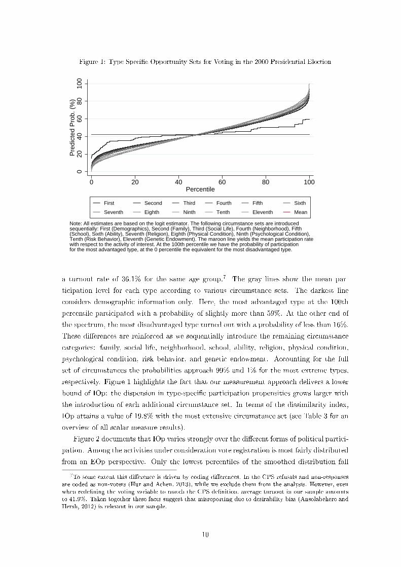
Figure 1: Type-Specic Opportunity Sets for Voting in the 2000 Presidential Election
020
4060
8010
0P
redi
cted
Pro
b. (
%)
0 20 40 60 80 100Percentile
First Second Third Fourth Fifth Sixth
Seventh Eighth Ninth Tenth Eleventh Mean
Note: All estimates are based on the logit estimator. The following circumstance sets are introducedsequentially: First (Demographics), Second (Family), Third (Social Life), Fourth (Neighborhood), Fifth(School), Sixth (Ability), Seventh (Religion), Eighth (Physical Condition), Ninth (Psychological Condition),Tenth (Risk Behavior), Eleventh (Genetic Endowment). The maroon line yields the mean participation ratewith respect to the activity of interest. At the 100th percentile we have the probability of participationfor the most advantaged type, at the 0 percentile the equivalent for the most disadvantaged type.
a turnout rate of 36.1% for the same age group.7 The gray lines show the mean par-
ticipation level for each type according to various circumstance sets. The darkest line
considers demographic information only. Here, the most advantaged type at the 100th
percentile participated with a probability of slightly more than 59%. At the other end of
the spectrum, the most disadvantaged type turned out with a probability of less than 16%.
These dierences are reinforced as we sequentially introduce the remaining circumstance
categories: family, social life, neighborhood, school, ability, religion, physical condition,
psychological condition, risk behavior, and genetic endowment. Accounting for the full
set of circumstances the probabilities approach 99% and 1% for the most extreme types,
respectively. Figure 1 highlights the fact that our measurement approach delivers a lower
bound of IOp: the dispersion in type-specic participation propensities grows larger with
the introduction of each additional circumstance set. In terms of the dissimilarity index,
IOp attains a value of 19.8% with the most extensive circumstance set (see Table 3 for an
overview of all scalar measure results).
Figure 2 documents that IOp varies strongly over the dierent forms of political partici-
pation. Among the activities under consideration vote registration is most fairly distributed
from an EOp perspective. Only the lowest percentiles of the smoothed distribution fall
7To some extent this dierence is driven by coding dierences. In the CPS refusals and non-responsesare coded as non-voters (Hur and Achen, 2013), while we exclude them from the analysis. However, evenwhen redening the voting variable to match the CPS denition, average turnout in our sample amountsto 41.9%. Taken together these facts suggest that misreporting due to desirability bias (Ansolabehere andHersh, 2012) is relevant in our sample.
10
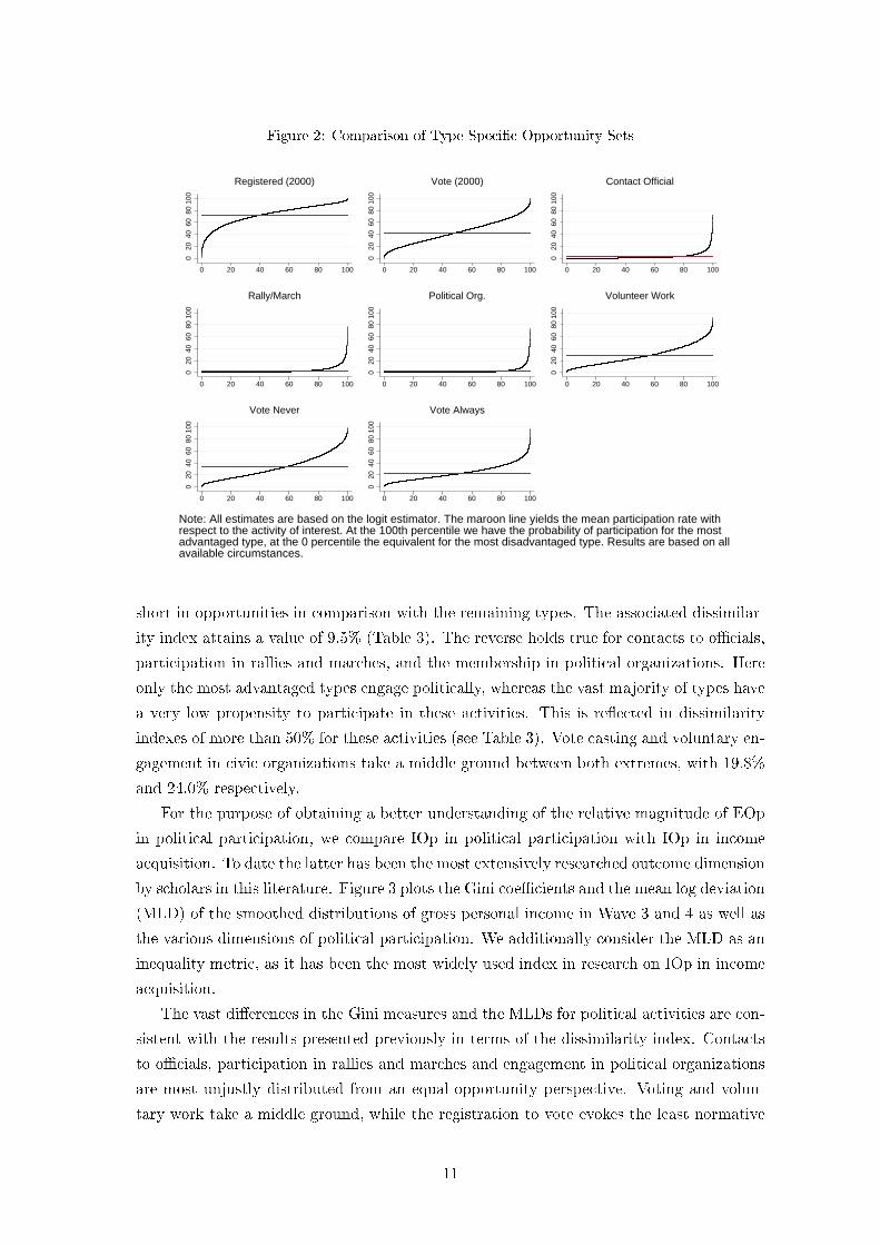
Figure 2: Comparison of Type-Specic Opportunity Sets
020
4060
8010
0
0 20 40 60 80 100
Registered (2000)
020
4060
8010
0
0 20 40 60 80 100
Vote (2000)
020
4060
8010
0
0 20 40 60 80 100
Contact Official0
2040
6080
100
0 20 40 60 80 100
Rally/March
020
4060
8010
0
0 20 40 60 80 100
Political Org.
020
4060
8010
0
0 20 40 60 80 100
Volunteer Work
020
4060
8010
0
0 20 40 60 80 100
Vote Never
020
4060
8010
0
0 20 40 60 80 100
Vote Always
Note: All estimates are based on the logit estimator. The maroon line yields the mean participation rate withrespect to the activity of interest. At the 100th percentile we have the probability of participation for the mostadvantaged type, at the 0 percentile the equivalent for the most disadvantaged type. Results are based on allavailable circumstances.
short in opportunities in comparison with the remaining types. The associated dissimilar-
ity index attains a value of 9.5% (Table 3). The reverse holds true for contacts to ocials,
participation in rallies and marches, and the membership in political organizations. Here
only the most advantaged types engage politically, whereas the vast majority of types have
a very low propensity to participate in these activities. This is reected in dissimilarity
indexes of more than 50% for these activities (see Table 3). Vote casting and voluntary en-
gagement in civic organizations take a middle ground between both extremes, with 19.8%
and 24.0% respectively.
For the purpose of obtaining a better understanding of the relative magnitude of EOp
in political participation, we compare IOp in political participation with IOp in income
acquisition. To date the latter has been the most extensively researched outcome dimension
by scholars in this literature. Figure 3 plots the Gini coecients and the mean log deviation
(MLD) of the smoothed distributions of gross personal income in Wave 3 and 4 as well as
the various dimensions of political participation. We additionally consider the MLD as an
inequality metric, as it has been the most widely used index in research on IOp in income
acquisition.
The vast dierences in the Gini measures and the MLDs for political activities are con-
sistent with the results presented previously in terms of the dissimilarity index. Contacts
to ocials, participation in rallies and marches and engagement in political organizations
are most unjustly distributed from an equal-opportunity perspective. Voting and volun-
tary work take a middle ground, while the registration to vote evokes the least normative
11
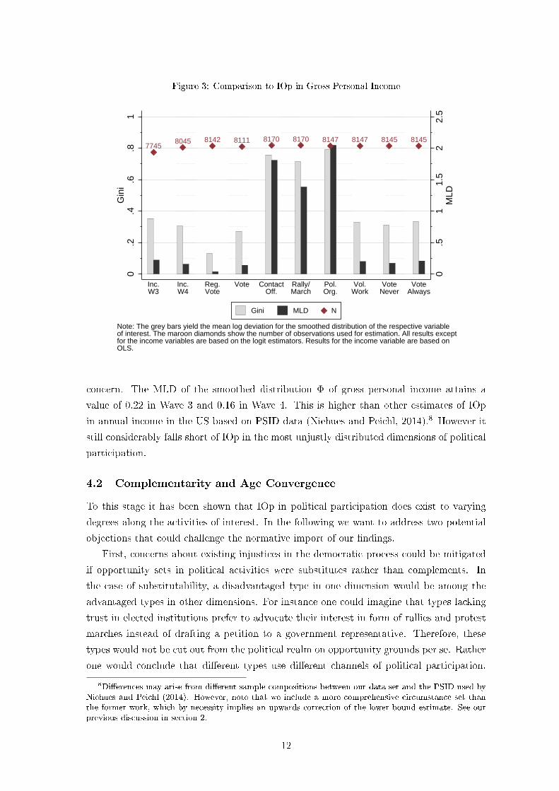
Figure 3: Comparison to IOp in Gross Personal Income
77458142 8111 8170 8170 8147 81478045 8145 8145
0.5
11.
52
2.5
MLD
0.2
.4.6
.81
Gin
i
Inc.W3
Inc.W4
Reg.Vote
Vote ContactOff.
Rally/March
Pol.Org.
Vol.Work
VoteNever
VoteAlways
Gini MLD N
Note: The grey bars yield the mean log deviation for the smoothed distribution of the respective variableof interest. The maroon diamonds show the number of observations used for estimation. All results exceptfor the income variables are based on the logit estimators. Results for the income variable are based onOLS.
concern. The MLD of the smoothed distribution Φ of gross personal income attains a
value of 0.22 in Wave 3 and 0.16 in Wave 4. This is higher than other estimates of IOp
in annual income in the US based on PSID data (Niehues and Peichl, 2014).8 However it
still considerably falls short of IOp in the most unjustly distributed dimensions of political
participation.
4.2 Complementarity and Age Convergence
To this stage it has been shown that IOp in political participation does exist to varying
degrees along the activities of interest. In the following we want to address two potential
objections that could challenge the normative import of our ndings.
First, concerns about existing injustices in the democratic process could be mitigated
if opportunity sets in political activities were substitutes rather than complements. In
the case of substitutability, a disadvantaged type in one dimension would be among the
advantaged types in other dimensions. For instance one could imagine that types lacking
trust in elected institutions prefer to advocate their interest in form of rallies and protest
marches instead of drafting a petition to a government representative. Therefore, these
types would not be cut out from the political realm on opportunity grounds per se. Rather
one would conclude that dierent types use dierent channels of political participation.
8Dierences may arise from dierent sample compositions between our data set and the PSID used byNiehues and Peichl (2014). However, note that we include a more comprehensive circumstance set thanthe former work, which by necessity implies an upwards correction of the lower bound estimate. See ourprevious discussion in section 2.
12
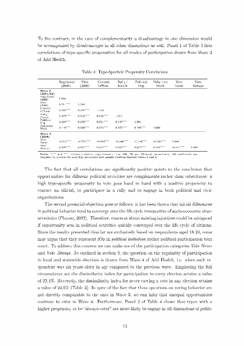
To the contrary, in the case of complementarity a disadvantage in one dimension would
be accompanied by disadvantages in all other dimensions as well. Panel 1 of Table 4 lists
correlations of type-specic propensities for all modes of participation drawn from Wave 3
of Add Health.
Table 4: Type-Speccic Propensity Correlations
Registered(2000)
Vote(2000)
ContactOcial
Rally/March
PoliticalOrg.
VolunteerWork
VoteNever
VoteAlways
Wave 3(2001/02)Registered(2000) 1.000
Vote(2000) 0.761∗∗∗ 1.000
ContactOcial 0.208∗∗∗ 0.296∗∗∗ 1.000
Rally/March 0.289∗∗∗ 0.346∗∗∗ 0.341∗∗∗ 1.000
PoliticalOrg. 0.183∗∗∗ 0.229∗∗∗ 0.324∗∗∗ 0.246∗∗∗ 1.000
VolunteerWork 0.449∗∗∗ 0.539∗∗∗ 0.345∗∗∗ 0.375∗∗∗ 0.295∗∗∗ 1.000
Wave 4(2008)VoteNever -0.704∗∗∗ -0.776∗∗∗ -0.254∗∗∗ -0.344∗∗∗ -0.194∗∗∗ -0.509∗∗∗ 1.000
VoteAlways 0.500∗∗∗ 0.565∗∗∗ 0.209∗∗∗ 0.323∗∗∗ 0.213∗∗∗ 0.338∗∗∗ -0.641∗∗∗ 1.000
Note: ∗,∗∗ and ∗∗∗ indicate statistical signicance at the 10%, 5% and 1%-level, respectively. All coecients areweighted to account for sampling procedure and sample attrition through waves 3 and 4.
The fact that all correlations are signicantly positive points to the conclusion that
opportunities for dierent political activities are complements rather than substitutes: a
high type-specic propensity to vote goes hand in hand with a positive propensity to
contact an ocial, to participate in a rally and to engage in both political and civic
organizations.
The second potential objection goes as follows: it has been shown that initial dierences
in political behavior tend to converge over the life cycle irrespective of socio-economic char-
acteristics (Plutzer, 2002). Therefore, concerns about existing injustices could be mitigated
if opportunity sets in political activities quickly converged over the life cycle of citizens.
Since the results presented thus far are exclusively based on respondents aged 18-24, some
may argue that they represent IOp in political initiation rather political participation tout
court. To address this concern we can make use of the participation categories Vote Never
and Vote Always. As outlined in section 3, the question on the regularity of participation
in local and statewide elections is drawn from Wave 4 of Add Health, i.e. when each re-
spondent was six years older in age compared to the previous wave. Employing the full
circumstance set the dissimilarity index for participation in every election attains a value
of 22.4%. Reversely, the dissimilarity index for never casting a vote in any election attains
a value of 24.5% (Table 3). In spite of the fact that these questions on voting behavior are
not directly comparable to the ones in Wave 3, we can infer that unequal opportunities
continue to exist in Wave 4. Furthermore, Panel 2 of Table 4 shows that types with a
higher propensity to be always-voter are more likely to engage in all dimensions of politi-
13
cal activity measured in Wave 3. Reversely, being a never-voter is consistently negatively
correlated with political engagement in the previous wave.
To conclude, neither is it the case that political opportunities across dierent activities
substitute each other, nor do type-specic propensities to engage politically quickly con-
verge over time. Thus the normative concern implicit in our previous results remains in
place.
4.3 Genetics and EOp
As mentioned previously, this is the rst work that explicitly exploits genetic variation
in the measurement of EOp. Therefore, we will devote this section to a more thorough
discussion of the inuence of genetic circumstances on EOp.
There is philosophical controversy on whether the genetic endowment of a person pro-
vides a ground for compensation. Clearly genes are part of the natural lottery and are
beyond individual control. Yet some argue that the ethical principle of self-ownership
takes priority over the value of equal opportunities, leading to the conclusion that people
have a legitimate claim on life outcomes rooted in their genetic make-up. For instance,
in his seminal contribution Rawls (1971) argues that fair equality of opportunity only
requires compensation for social circumstances, but not for natural circumstances.
To date the empirical literature on EOp at most accounts for proxy variables for genetic
circumstances. Björklund et al. (2012), for instance, use IQ measures from the Swedish
Military Enlistment Battery measured at age 18. Yet as the authors remark, it is not
clear to what extent such ability measures reect nature (genetic endowments) or nurture
(childhood circumstances). In humans genetic information is stored on 46 chromosomes,
half of which are received from each of the biological parents respectively. Chromosomes
contain chains of the macromolecule deoxyribonucleic acid (DNA). DNA is composed of two
strands of sugar and phosphate molecules that are connected by corresponding base pairs.
Adenine (A) always pairs with thymine (T) while guanine (G) always pairs with cytosine
(C). The two strands coil around each other to form the famous double helix structure. In
total, one set of chromosomes consists of 3.3bn base pairs of which 3% are protein coding
(exons), whereas the remainder is believed to have a regulatory function (introns). Genes
are segments of the DNA that are involved in the coding of proteins. Genetic dierences
are denoted as alleles (or polymorphisms). As one chromosome is inherited of each parent,
children also inherit one allele for a particular gene from each parent.
Add Health provides two dierent sorts of genetic markers:9 variable number tandem
repeats (VNTR) for six genes (MAOA, DRD4, DAT1, DRD5, MAOCA1, HTTLPR) and
single-nucleotide polymorphisms (SNP) in the genes HTTLPR, DRD2, COMT and 5HTT.
VNTRs code repeats of base pair sequences on a gene. For instance, the enzyme monoamine
oxidase A (MAOA) is involved in the degradation of serotonin in the brain. It is coded
9For more information on genetic markers in Add Health see Smolen et al. (2013)
14
on the gene MAOA, which contains a 30 base pair sequence, which varies between 2 and 5
repeat units depending on the allelic expression. The two repeat (2R) and the three repeat
(3R) expression are believed to be more ecient in the transcription of the necessary amino
acids for the formation of the MAOA enzyme than the alternative expressions. Deciencies
in the degradation of serotonin have been shown to be negatively correlated with pro-social
behaviors, which in turn led political scientists to hypothesize that low-expressing MAOA
VNTR's lead to lower degrees of political participation (Fowler and Dawes, 2008). Instead
of recording genetic variation with respect to base pair repeats, SNPs indicate alternations
in the base pairs at a particular locus. For instance, the SNP rs12945042 refers to the 5HTT
gene. At this particular location of the DNA, the majority base pair C-G is replaced by a
T-A base pair in the minority allele. As MAOA, 5HTT is involved in the degradation of
serotonin. Thus, to the extent that one allele is more transcriptionally ecient than the
other, we would expect dierential political participation across the carriers of the dierent
allele expressions. Note that in contrast to VNTRs genetic variation due to SNPs can take
at most three expressions. A person can inherit the minor allele from none, one, or both
biological parents. For one gene (HTTLPR) we use a combination of both VNTRs and
SNPs. Previous research has shown that a minor allele SNP (G) on long versions of the
HTTLPR VNRT is less active than long versions with the more common variant (A). Thus
shorter versions of this VNTR should be analyzed jointly with long versions that carry the
minor allele SNP. The more active alleles are indicated as L' while the less active alleles
are coded as S' (see Table 10).
In general the genetic information in Add Health is relatively limited. To date genome-
wide sequencing has detected 84.7mn SNPs and 60,000 structural variants of which VNTRs
are a subset (Altshuler et al., 2015). Thus, the genetic circumstance set employed in this
study is far from capturing the entirety of genetic variation causally related to political
participation.10
Table 5 shows results on IOp in political participation with respect to dierent cir-
cumstance scenarios. The rst line of each panel repeats the benchmark IOp measure
accounting for all available circumstances (see Table 3) for each dimension of interest.
Drawing on bootstrapped standard errors, we contrast this measure with two alternative
scenarios.
First, we calculate IOp using circumstance sets based on genetic information only.
We see that a relatively small fraction of IOp is explained independently by the set of
available genetic markers. This nding is unsurprising in view of the paucity of genetic
information in our data set. Political participation is a highly polygenic trait, i.e. a large
amount of genetic variants with very small individual eect sizes explain the heritability
10Obviously this will lead us to underestimate the impact of genetic circumstances. To some extent thisdownward bias is mitigated by the fact that alleles are in linkage disequilibrium. This property states thatthe correlation of alleles increases with their proximity on the respective chromosome (Altshuler et al.,2015). It will bias the point estimates of the specic genetic variants upwards but brings us closer to thetrue amount of variation in political participation explained by genetic information.
15
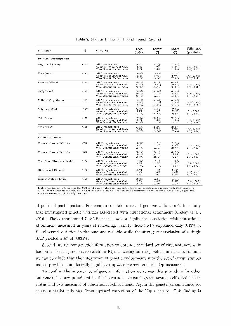
Table 5: Genetic Inuence (Bootstrapped Results)
Outcome N Circ. SetDiss.Index
LowerCI
UpperCI
Dierence(p-value)
Political Participation
Registered (2000) 8142 All Circumstances 9.5% 8.7% 10.4%Genetic Endowment Only 2.5% 1.9% 3.2% 7.0(0.000)W/o Genetic Endowment 9.2% 8.3% 10.0% 0.4(0.000)
Vote (2000) 8111 All Circumstances 19.8% 18.4% 21.2%Genetic Endowment Only 4.8% 3.6% 5.9% 15.0(0.000)W/o Genetic Endowment 19.2% 17.8% 20.6% 0.6(0.001)
Contact Ocial 8170 All Circumstances 59.7% 55.2% 64.1%Genetic Endowment Only 23.6% 18.4% 28.8% 36.0(0.000)W/o Genetic Endowment 56.3% 51.7% 60.9% 3.3(0.001)
Rally/March 8170 All Circumstances 55.4% 50.6% 60.2%Genetic Endowment Only 20.6% 15.1% 26.1% 34.8(0.000)W/o Genetic Endowment 51.7% 47.1% 56.3% 3.7(0.000)
Political Organization 8147 All Circumstances 63.0% 56.9% 69.1%Genetic Endowment Only 23.4% 16.7% 30.1% 39.6(0.000)W/o Genetic Endowment 58.8% 52.9% 64.7% 4.2(0.001)
Volunteer Work 8147 All Circumstances 24.0% 22.2% 25.8%Genetic Endowment Only 5.9% 4.3% 7.4% 18.1(0.000)W/o Genetic Endowment 23.3% 21.5% 25.0% 0.7(0.004)
Vote Always 8145 All Circumstances 22.4% 20.5% 24.4%Genetic Endowment Only 9.1% 7.3% 11.0% 13.3(0.000)W/o Genetic Endowment 21.3% 19.3% 23.2% 1.1(0.001)
Vote Never 8145 All Circumstances 24.5% 23.0% 26.1%Genetic Endowment Only 7.4% 5.9% 8.9% 17.1(0.000)W/o Genetic Endowment 23.8% 22.3% 25.4% 0.7(0.002)
Other Outcomes
Personal Income W3 (k$) 7745 All Circumstances 23.3% 18.9% 27.8%Genetic Endowment Only 3.0% 1.2% 4.8% 20.3(0.000)W/o Genetic Endowment 21.7% 17.4% 26.0% 1.7(0.007)
Personal Income W4 (k$) 8045 All Circumstances 30.7% 27.1% 34.2%Genetic Endowment Only 10.6% 8.4% 12.9% 20.1(0.000)W/o Genetic Endowment 28.8% 25.4% 32.2% 1.9(0.000)
Very Good/Excellent Health 8180 All Circumstances 14.5% 13.4% 15.6%Genetic Endowment Only 3.6% 2.7% 4.5% 10.9(0.000)W/o Genetic Endowment 14.2% 13.1% 15.3% 0.3(0.020)
High School Diploma 8180 All Circumstances 4.7% 4.1% 5.4%Genetic Endowment Only 1.4% 1.0% 1.8% 3.3(0.000)W/o Genetic Endowment 4.6% 3.9% 5.2% 0.1(0.004)
(Some) Tertiary Educ. 8179 All Circumstances 18.3% 17.2% 19.4%Genetic Endowment Only 4.6% 3.8% 5.5% 13.7(0.000)W/o Genetic Endowment 18.1% 17.0% 19.2% 0.2(0.015)
Note: Condence intervals at the 95%-level and p-values are calculated based on bootstrapped results with 1000 draws. p-values refer to one-sided tests, as to whether the inclusion of the respective circumstance set causes a statistically signicantupwards correction of the IOp measure.
of political participation. For comparison take a recent genome-wide association study
that investigated genetic variants associated with educational attainment (Okbay et al.,
2016). The authors found 74 SNPs that showed a signicant association with educational
attainment measured in years of schooling. Jointly these SNPs explained only 0.43% of
the observed variation in the outcome variable while the strongest association of a single
SNP yielded a R2 of 0.035%.
Second, we remove genetic information to obtain a standard set of circumstances as it
has been used in previous research on IOp. Focusing on the p-values in the last column,
we can conclude that the integration of genetic endowments into the set of circumstances
indeed provides a statistically signicant upward correction of all IOp measures.
To conrm the importance of genetic information we repeat this procedure for other
outcomes that are prominent in the literature: personal gross income, self-rated health
status and two measures of educational achievement. Again the genetic circumstance set
causes a statistically signicant upward correction of the IOp measure. This nding is
16
particularly relevant as most applied research on EOp relies on a lower bound estimation
method (Niehues and Peichl, 2014). The information we use with respect to childhood cir-
cumstances is already comprehensive in comparison to previous works on IOp. Thus one
could have expected that much of the genetic variation was already reected in the set of
childhood circumstances which are shaped subsequent to the natural lottery of distribut-
ing genetic endowments. The fact that genetic information still provides an independent
upward correction of IOp indicates that the increasing availability of large-scale genetic
data sets may be fruitfully exploited in future empirical works of IOp.11 Add Health it-
self plans to sequence its available saliva samples, which will make available genome-wide
information that goes far beyond the candidate genes used in this study. Once available,
this data could be used to construct polygenic risk scores (Dudbridge, 2013) that compile
relevant genetic information for thousands of SNPs into one index variable.
4.4 Underlying Mechanisms
It is important to note that it is beyond the ambit of the current analysis to establish
causal claims on the inuence of specic circumstances on the existing political opportu-
nity structure in the US. To guide policy, however, it is indispensable to move beyond the
exploratory approach of the current analysis and to gain an understanding of the mecha-
nisms at play.12 After all, is it neighborhood characteristics or demographics (or any other
factor) that drives the opportunity gap in political participation? Depending on the answer
policy recommendations may be radically dierent. To respond to this quest we rely on
two decomposition exercises. First, we use the Shapley value decomposition methodology
proposed by Shorrocks (2012) to display which circumstance group provides the strongest
contribution to IOp as presented in Table 3. Second, we introduce selected eort variables
into the analytic framework for the purpose of analyzing the extent to which the dierent
circumstance groups exert an indirect inuence through individual eort. Hereby we rely
on a recent methodology developed by Gelbach (2016).
In contrast to other decomposition methodologies, the Shapley value procedure over-
comes the issue of path-dependency in evaluating dierent contribution factors. Therefore
it delivers unbiased and additive decomposition results, i.e. the calculated contributions
sum to the total measure of inequality. We implement the decomposition as follows. There
11Furthermore it is conceivable to use genetic data to rene empirical estimates of IOp with respect todierent philosophical accounts. To the extent that childhood circumstances are correlated with geneticendowments, current estimates of IOp implicitly treat returns to genetic endowments as ethically objec-tionable and thus take a contested normative standpoint. To correct for this shortcoming one could adjustthe empirical framework used in this work. Similar to our approach one would use genetic circumstances ascontrols in equation 2. However subsequently they would be neglected in the construction of the smootheddistribution (equation 3). The result would be the true measure of IOp net of genetic inuence as coe-cients on childhood circumstances were no longer biased by correlations with antecedent genetic factors.This procedure, however, requires a data set with genetic information akin to the one used for the purposeof this analysis.
12For instance Kanbur and Wagsta (2014) question the policy relevance of the existing EOp literatureon these grounds.
17
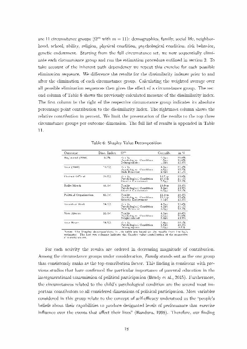
are 11 circumstance groups (Ωm with m = 11): demographics, family, social life, neighbor-
hood, school, ability, religion, physical condition, psychological condition, risk behavior,
genetic endowment. Starting from the full circumstance set, we now sequentially elimi-
nate each circumstance group and run the estimation procedure outlined in section 2. To
take account of the inherent path dependency we repeat this exercise for each possible
elimination sequence. We dierence the results for the dissimilarity indexes prior to and
after the elimination of each circumstance group. Calculating the weighted average over
all possible elimination sequences then gives the eect of a circumstance group. The sec-
ond column of Table 6 shows the previously calculated measure of the dissimilarity index.
The rst column to the right of the respective circumstance group indicates its absolute
percentage point contribution to the dissimilarity index. The rightmost column shows the
relative contribution in percent. We limit the presentation of the results to the top three
circumstance groups per outcome dimension. The full list of results is appended in Table
11.
Table 6: Shapley Value Decomposition
Outcome Diss. Index Ωm Contrib. in %
Registered (2000) 9.5% Family 2.0pp 21.0%Psychological Condition 1.5pp 16.0%Demographics 1.2pp 12.5%
Vote (2000) 19.8% Family 4.0pp 20.3%Psychological Condition 3.5pp 17.7%Risk Behavior 2.0pp 10.1%
Contact Ocial 59.7% Family 13.7pp 23.0%Psychological Condition 10.4pp 17.4%Genetic Endowment 7.5pp 12.5%
Rally/March 55.4% Family 13.0pp 23.5%Psychological Condition 8.3pp 14.9%Genetic Endowment 6.7pp 12.2%
Political Organization 63.0% Family 11.5pp 18.3%Psychological Condition 11.2pp 17.8%Genetic Endowment 7.7pp 12.3%
Volunteer Work 24.0% Family 4.7pp 19.8%Psychological Condition 4.2pp 17.4%Risk Behavior 3.0pp 12.5%
Vote Always 22.4% Family 4.2pp 18.6%Psychological Condition 3.6pp 16.0%Neighborhood 3.3pp 14.9%
Vote Never 24.5% Family 5.4pp 22.2%Psychological Condition 4.5pp 18.3%Demographics 2.2pp 9.1%
Note: The Shapley decompositions in this table are based on the results from the logitestimator. The last two columns indicate the Shapley value contribution of the respectivecircumstance set.
For each activity the results are ordered in decreasing magnitude of contribution.
Among the circumstance groups under consideration, Family stands out as the one group
that consistently ranks as the top contribution factor. This nding is consistent with pre-
vious studies that have conrmed the particular importance of parental education in the
intergenerational transmission of political participation (Brady et al., 2015). Furthermore,
the circumstances related to the child's psychological condition are the second most im-
portant contributors to all considered dimensions of political participation. Most variables
considered in this group relate to the concept of self-ecacy understood as the people's
beliefs about their capabilities to produce designated levels of performance that exercise
inuence over the events that aect their lives (Bandura, 1998). Therefore, our nding
18
conrms previous research that considers a sense of political self-ecacy as one of the
determining factors of political participation (Finkel, 1985). To the contrary, given its
prominence in the academic literature (Jones-Correa and Leal, 2001) the small inuence
of the religious background of the respondents is striking. A similar conclusion holds for
the categories Social Life, School, Ability and Physical Condition, all of which account for
less than 10% of the explained variation in each activity of interest.
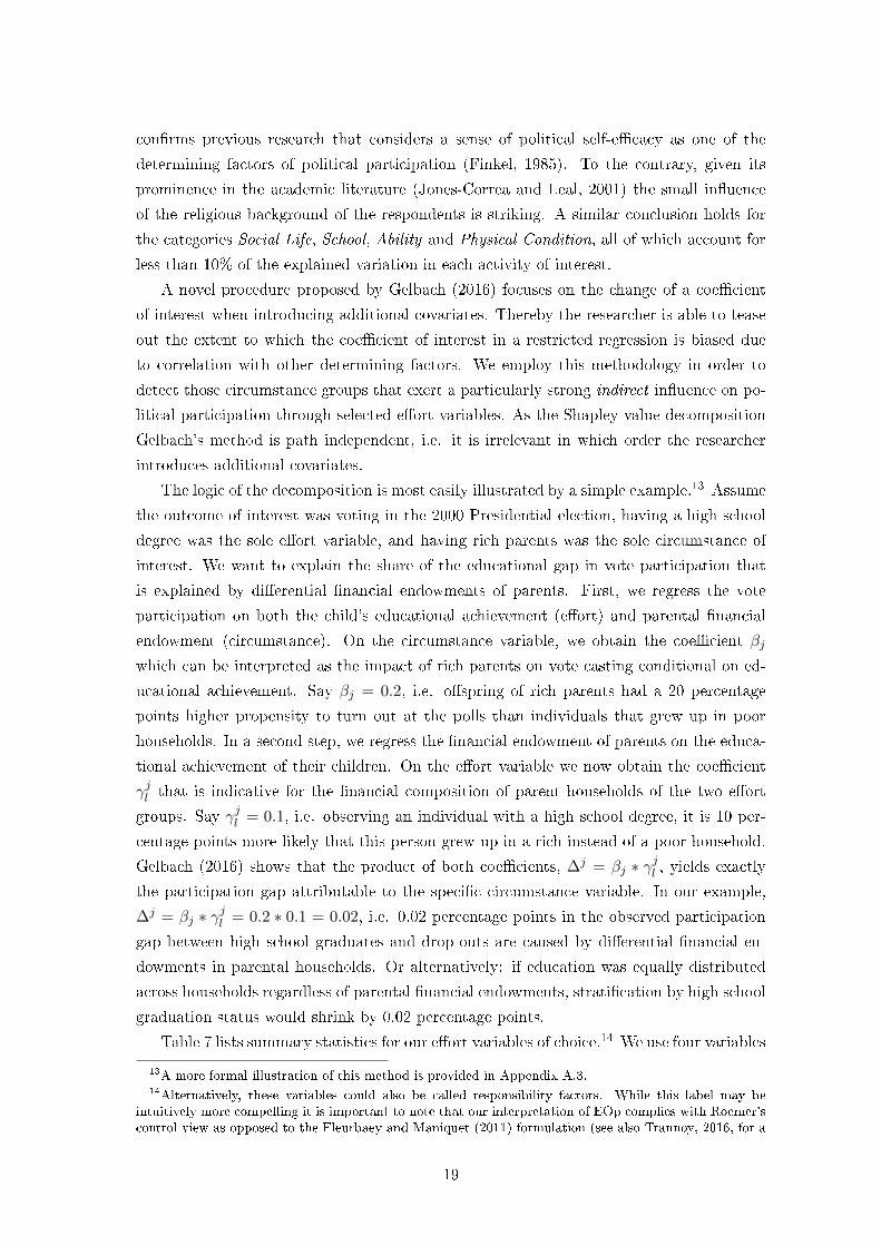
A novel procedure proposed by Gelbach (2016) focuses on the change of a coecient
of interest when introducing additional covariates. Thereby the researcher is able to tease
out the extent to which the coecient of interest in a restricted regression is biased due
to correlation with other determining factors. We employ this methodology in order to
detect those circumstance groups that exert a particularly strong indirect inuence on po-
litical participation through selected eort variables. As the Shapley value decomposition
Gelbach's method is path independent, i.e. it is irrelevant in which order the researcher
introduces additional covariates.
The logic of the decomposition is most easily illustrated by a simple example.13 Assume
the outcome of interest was voting in the 2000 Presidential election, having a high school
degree was the sole eort variable, and having rich parents was the sole circumstance of
interest. We want to explain the share of the educational gap in vote participation that
is explained by dierential nancial endowments of parents. First, we regress the vote
participation on both the child's educational achievement (eort) and parental nancial
endowment (circumstance). On the circumstance variable, we obtain the coecient βj
which can be interpreted as the impact of rich parents on vote casting conditional on ed-
ucational achievement. Say βj = 0.2, i.e. ospring of rich parents had a 20 percentage
points higher propensity to turn out at the polls than individuals that grew up in poor
households. In a second step, we regress the nancial endowment of parents on the educa-
tional achievement of their children. On the eort variable we now obtain the coecient
γjl that is indicative for the nancial composition of parent households of the two eort
groups. Say γjl = 0.1, i.e. observing an individual with a high school degree, it is 10 per-
centage points more likely that this person grew up in a rich instead of a poor household.
Gelbach (2016) shows that the product of both coecients, ∆j = βj ∗ γjl , yields exactlythe participation gap attributable to the specic circumstance variable. In our example,
∆j = βj ∗ γjl = 0.2 ∗ 0.1 = 0.02, i.e. 0.02 percentage points in the observed participation
gap between high school graduates and drop-outs are caused by dierential nancial en-
dowments in parental households. Or alternatively: if education was equally distributed
across households regardless of parental nancial endowments, stratication by high school
graduation status would shrink by 0.02 percentage points.
Table 7 lists summary statistics for our eort variables of choice.14 We use four variables
13A more formal illustration of this method is provided in Appendix A.3.14Alternatively, these variables could also be called responsibility factors. While this label may be
intuitively more compelling it is important to note that our interpretation of EOp complies with Roemer'scontrol view as opposed to the Fleurbaey and Maniquet (2011) formulation (see also Trannoy, 2016, for a
19
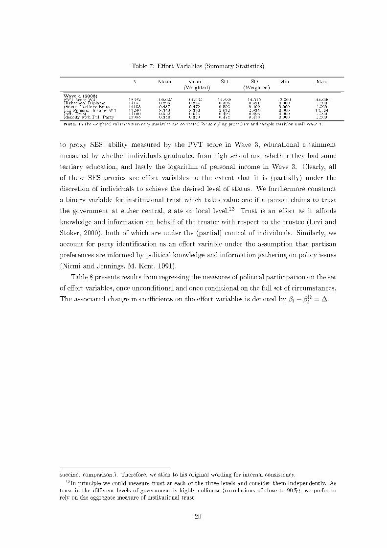
Table 7: Eort Variables (Summary Statistics)
N Mean Mean(Weighted)
SD SD(Weighted)
Min Max
Wave 4 (2008)PVT Score W3 18392 100.025 101.634 14.930 14.515 13.000 146.000Highschool Diploma 14151 0.896 0.884 0.305 0.321 0.000 1.000(Some) Tertiary Educ. 14153 0.487 0.472 0.500 0.499 0.000 1.000Log Personal Income W3 13280 8.340 8.330 2.632 2.635 0.000 13.124Inst. Trust 14100 0.532 0.544 0.499 0.498 0.000 1.000Identify with Pol. Party 13955 0.348 0.329 0.476 0.470 0.000 1.000
Note: In the weighted columns summary statistics are corrected for sampling procedure and sample attrition until Wave 3.
to proxy SES: ability measured by the PVT score in Wave 3, educational attainment
measured by whether individuals graduated from high school and whether they had some
tertiary education, and lastly the logarithm of personal income in Wave 3. Clearly, all
of these SES proxies are eort variables to the extent that it is (partially) under the
discretion of individuals to achieve the desired level of status. We furthermore construct
a binary variable for institutional trust which takes value one if a person claims to trust
the government at either central, state or local level.15 Trust is an eort as it aords
knowledge and information on behalf of the truster with respect to the trustee (Levi and
Stoker, 2000), both of which are under the (partial) control of individuals. Similarly, we
account for party identication as an eort variable under the assumption that partisan
preferences are informed by political knowledge and information gathering on policy issues
(Niemi and Jennings, M. Kent, 1991).
Table 8 presents results from regressing the measures of political participation on the set
of eort variables, once unconditional and once conditional on the full set of circumstances.
The associated change in coecients on the eort variables is denoted by βl − βΩl = ∆.
succinct comparison.). Therefore, we stick to his original wording for internal consistency.15In principle we could measure trust at each of the three levels and consider them independently. As
trust in the dierent levels of government is highly collinear (correlations of close to 90%), we prefer torely on the aggregate measure of institutional trust.
20
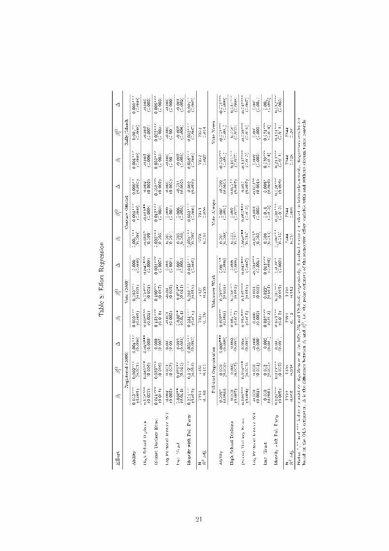
Table8:Eort
Regression
Eort
βl
βΩ l
∆βl
βΩ l
∆βl
βΩ l
∆βl
βΩ l
∆
Registered(2000)
Vote
(2000)
ContactOcial
Rally/March
Ability
0.003***
0.002***
0.001***
0.003***
0.003***
0.000
0.001***
0.001***
0.000**
0.001***
0.001**
0.000***
(0.001)
(0.001)
(0.000)
(0.001)
(0.001)
(0.000)
(0.000)
(0.000)
(0.000)
(0.000)
(0.000)
(0.000)
HighSchoolDiploma
0.108***
0.085***
0.023***
0.098***
0.059***
0.040***
-0.016*
-0.018**
0.002
-0.007
-0.007
-0.000
(0.027)
(0.026)
(0.008)
(0.021)
(0.021)
(0.009)
(0.009)
(0.009)
(0.003)
(0.006)
(0.007)
(0.003)
(Some)Tertiary
Educ.
0.091***
0.083***
0.008
0.138***
0.100***
0.038***
0.023***
0.016***
0.008***
0.030***
0.022***
0.008***
(0.014)
(0.016)
(0.007)
(0.016)
(0.017)
(0.007)
(0.005)
(0.005)
(0.003)
(0.005)
(0.005)
(0.003)
LogPersonalIncomeW3
0.002
0.001
0.001
-0.001
-0.001
0.001
0.001
0.000
0.000
-0.000
-0.000
-0.000
(0.003)
(0.002)
(0.001)
(0.003)
(0.003)
(0.001)
(0.001)
(0.001)
(0.000)
(0.001)
(0.001)
(0.000)
Inst.Trust
0.030**
0.028**
0.002
0.030**
0.029**
0.001
0.005
0.006
-0.001
-0.003
-0.002
-0.001
(0.014)
(0.014)
(0.005)
(0.014)
(0.014)
(0.005)
(0.005)
(0.005)
(0.002)
(0.005)
(0.006)
(0.002)
Identify
withPol.Party
0.204***
0.172***
0.033***
0.331***
0.288***
0.043***
0.035***
0.033***
0.002
0.036***
0.032***
0.004**
(0.013)
(0.013)
(0.005)
(0.016)
(0.016)
(0.005)
(0.006)
(0.006)
(0.002)
(0.006)
(0.007)
(0.002)
N7353
7353
7327
7327
7373
7373
7372
7372
R2adj.
0.103
0.164
0.170
0.235
0.033
0.056
0.027
0.044
PoliticalOrganization
VolunteerWork
Vote
Always
Vote
Never
Ability
0.000*
0.000
0.000***
0.002***
0.002***
0.001**
0.001
0.001
-0.000
-0.003***
-0.002***
-0.001***
(0.000)
(0.000)
(0.000)
(0.001)
(0.001)
(0.000)
(0.000)
(0.001)
(0.000)
(0.001)
(0.001)
(0.000)
HighSchoolDiploma
-0.006
-0.003
-0.003
0.067***
0.058***
0.008
0.023
0.007
0.017**
-0.104***
-0.048*
-0.057***
(0.007)
(0.007)
(0.002)
(0.017)
(0.019)
(0.008)
(0.021)
(0.022)
(0.007)
(0.027)
(0.025)
(0.009)
(Some)Tertiary
Educ.
0.026***
0.023***
0.003
0.236***
0.187***
0.049***
0.069***
0.059***
0.010
-0.137***
-0.090***
-0.047***
(0.004)
(0.005)
(0.002)
(0.015)
(0.016)
(0.007)
(0.014)
(0.015)
(0.007)
(0.015)
(0.016)
(0.007)
LogPersonalIncomeW3
-0.000
0.000
-0.000
0.000
0.003
-0.003***
-0.005*
-0.003
-0.002**
0.002
0.001
0.001
(0.001)
(0.001)
(0.000)
(0.002)
(0.002)
(0.001)
(0.003)
(0.003)
(0.001)
(0.003)
(0.003)
(0.001)
Inst.Trust
-0.000
0.002
-0.002
0.036***
0.022*
0.014***
0.006
0.014
-0.008*
-0.060***
-0.061***
0.001
(0.005)
(0.004)
(0.001)
(0.013)
(0.014)
(0.004)
(0.013)
(0.013)
(0.004)
(0.014)
(0.014)
(0.005)
Identify
withPol.Party
0.020***
0.019***
0.001
0.073***
0.064***
0.010**
0.166***
0.138***
0.028***
-0.213***
-0.161***
-0.052***
(0.005)
(0.005)
(0.001)
(0.015)
(0.015)
(0.005)
(0.015)
(0.015)
(0.004)
(0.014)
(0.014)
(0.005)
N7359
7359
7359
7359
7344
7344
7344
7344
R2adj.
0.015
0.038
0.112
0.152
0.051
0.093
0.128
0.201
Note:
∗,∗
∗and
∗∗∗indicate
statisticalsignicanceatthe10%,5%and1%-level,respectively.Standard
errorsare
robustto
heteroskedasticity.Regressionresultsare
basedontheOLSestimator.
∆isthedierencebetweenβlandβ
Ω l,i.e.thepointestimate
oftherespectiveeortvariablewithandwithoutcircumstancecontrols.
21
It is noteworthy that SES as measured by ability and educational achievement are
strong determinants of political participation across most dimensions of activity, whereas
the independent inuence of personal income is negligible. Only with respect to being an
always-voter personal income exerts a small negative eect signicant at the 10%-level.16
However, this eect vanishes when controlling for individual circumstances. Similarly,
identication with a political party consistently exerts a signicant positive inuence on
political participation across all dimensions under consideration. The evidence on the in-
uence of institutional trust is somewhat mixed. People that claim to trust the government
on average register and vote with a higher probability of around 3 percentage points as
opposed to non-trusting individuals. Furthermore, more institutional trust is signicantly
correlated with a higher propensity for volunteer work and a lower probability of being
a never-voter. The coecients on all eort variables for which we nd a statistically
signicant relation to political participation are attenuated when accounting for the full
set of individual circumstances.
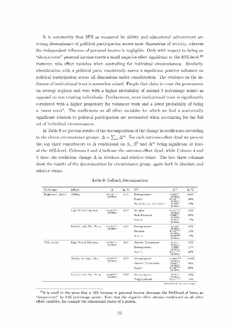
In Table 9 we present results of the decomposition of the change in coecients according
to the eleven circumstance groups: ∆ =∑
m ∆m. For each outcome-eort dyad we present
the top three contributors to ∆ conditional on βl, βΩl and ∆m being signicant at least
at the 10%-level. Columns 1 and 2 indicate the outcome-eort dyad, while Column 4 and
5 show the coecient change ∆ in absolute and relative terms. The last three columns
show the results of the decomposition by circumstance group, again both in absolute and
relative terms.
Table 9: Gelbach Decomposition
Outcome Eort ∆ in % Ωm ∆m in %
Registered (2000) Ability 0.001*** 37% Demographics 0.001** 130%(0.000) (0.001)
Family 0.001*** 56%(0.000)
Psychological Condition 0.000* 20%(0.000)
High School Diploma 0.023*** 21% Religion 0.007*** 33%(0.008) (0.002)
Risk Behavior 0.005** 24%(0.003)
School 0.004* 17%(0.002)
Identify with Pol. Party 0.033*** 16% Demographics 0.010* 30%(0.005) (0.005)
Religion 0.005*** 14%(0.002)
Family 0.005** 14%(0.002)
Vote (2000) High School Diploma 0.040*** 40% Genetic Endowment 0.031* 78%(0.009) (0.017)
Demographics -0.028* -72%(0.016)
Family 0.014*** 36%(0.005)
(Some) Tertiary Educ. 0.038*** 27% Demographics -0.049*** -130%(0.007) (0.017)
Genetic Endowment 0.035** 94%(0.018)
Family 0.026*** 68%(0.005)
Identify with Pol. Party 0.043*** 13% Demographics 0.012* 28%(0.005) (0.007)
Neighborhood 0.007*** 16%
Continued on next page
16It is small in the sense that a 10% increase in personal income decreases the likelihood of being analways-voter by 0.05 percentage points. Note that the negative eect obtains conditional on all othereort variables, for example the educational status of a person.
22
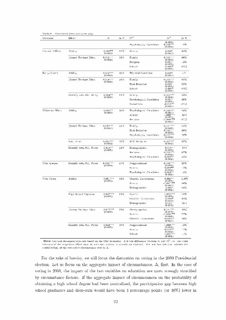
Table 9 Continued from previous page
Outcome Eort ∆ in % Ωm ∆m in %
(0.002)Psychological Condition 0.006*** 14%
(0.002)
Contact Ocial Ability 0.000** 19% Family 0.000* 49%(0.000) (0.000)
(Some) Tertiary Educ. 0.008*** 33% Family 0.005*** 66%(0.003) (0.002)
Religion 0.001* 14%(0.001)
School -0.001* -11%(0.001)
Rally/March Ability 0.000*** 36% Physical Condition 0.000* 7%(0.000) (0.000)
(Some) Tertiary Educ. 0.008*** 26% Family 0.005*** 67%(0.003) (0.002)
Risk Behavior 0.003* 33%(0.001)
School -0.001* -13%(0.001)
Identify with Pol. Party 0.004** 11% Family 0.002*** 50%(0.002) (0.001)
Psychological Condition 0.001* 28%(0.001)
Social Life -0.001** -26%(0.000)
Volunteer Work Ability 0.001** 30% Psychological Condition 0.000*** 59%(0.000) (0.000)
Ability -0.000*** -39%(0.000)
Religion -0.000*** -20%(0.000)
(Some) Tertiary Educ. 0.049*** 21% Family 0.017*** 35%(0.007) (0.005)
Risk Behavior 0.013*** 26%(0.003)
Psychological Condition 0.011*** 23%(0.004)
Inst. Trust 0.014*** 39% Risk Behavior 0.007*** 47%(0.004) (0.002)
Identify with Pol. Party 0.010** 13% Demographics -0.009** -96%(0.005) (0.004)
Religion 0.008*** 87%(0.002)
Psychological Condition 0.003** 35%(0.001)
Vote Always Identify with Pol. Party 0.028*** 17% Neighborhood 0.006*** 23%(0.004) (0.002)
Family 0.004** 15%(0.002)
Psychological Condition 0.004** 13%(0.001)
Vote Never Ability -0.001*** 34% Genetic Endowment 0.001** -118%(0.000) (0.001)
Family -0.001*** 94%(0.000)
Demographics -0.001* 93%(0.001)
High School Diploma -0.057*** 54% Family -0.025*** 44%(0.009) (0.005)
Genetic Endowment -0.025* 43%(0.013)
Demographics 0.023* -41%(0.013)
(Some) Tertiary Educ. -0.047*** 34% Demographics 0.044*** -93%(0.007) (0.017)
Family -0.036*** 77%(0.005)
Genetic Endowment -0.035** 74%(0.017)
Identify with Pol. Party -0.052*** 25% Neighborhood -0.008*** 14%(0.005) (0.002)
Family -0.006** 11%(0.002)
School -0.006*** 11%(0.001)
Note: Gelbach decompositions are based on the OLS estimator. ∆ is the dierence between βl and βΩl , i.e. the point
estimate of the respective eort variable with and without circumstance controls. The last two columns indicate the
contributions of the respective circumstance sets to ∆.
For the sake of brevity, we will focus the discussion on voting in the 2000 Presidential
election. Let us focus on the aggregate impact of circumstances, ∆, rst. In the case of
voting in 2000, the impact of the two variables on education are most strongly stratied
by circumstance factors. If the aggregate impact of circumstances on the probability of
obtaining a high school degree had been neutralized, the participation gap between high
school graduates and drop-outs would have been 4 percentage points (or 40%) lower in
23
this election. Analogously, the turnout gap between those who went to college and those
who did not would have been lowered by 3.8 percentage points (27%) if factors beyond
individual control had been uncorrelated to the probability of obtaining at least some ter-
tiary education. In general the results indicate that circumstances are a strong contributor
to the observed stratication of political participation by educational status, ranging from
21% in the dyad Tertiary Education-Volunteer Work up to 54% in the dyad High School
Diploma-Vote Never. In the case of party identication the relevant range lies somewhat
lower between 11% (Rally/March) and 25% (Vote Never). As regards institutional trust,
we detect only one statistically signicant relationship: a neutralization of circumstance
inuence on institutional trust would decrease the stratication of volunteer work between
trusting and non-trusting individuals by 1 percentage point (14%).
The last two columns of Table 9 further decompose the aggregate indirect impact of
circumstances through eort into the contributions of the eleven circumstance groups. It
is noteworthy that not all circumstance groups have a dis-equalizing indirect eect on
political opportunities in the US. To the contrary some circumstances mitigate the dier-
ential inuence other circumstance groups exert. For instance in the case of vote casting
in the 2000 Presidential election, genetics were the strongest contributors to the strati-
cation along the high school graduation divide. 78% of the 4 percentage point impact of
circumstances could be attributed to this circumstance group, i.e. stratication between
high school graduates and non-graduates would have been 3.1 percentage points lower
if genetics were uncorrelated to the probability of obtaining the respective degree. The
contrary conclusion holds for demographic circumstances. Had public policy been suc-
cessful in mitigating the inuence of demographics on the probability of graduating from
high school, the participation gap would have increased by 2.8 percentage points. This
result is mainly driven by dierential patterns in high school graduation rates and vote
casting across the sexes. Females had a lower participation (βj = −0.393) but higher
graduation rates (γjl = 0.073) than their male counterparts. Combining both estimates
∆j = −0.393 ∗ 0.073 = −0.029, which corresponds to the total equalizing contribution
of demographics (∆m = −0.028). A similar pattern is observable for the inuence of
demographics (and biological sex in particular) on vote casting via dierential tertiary ed-
ucation (∆j = −0.393 ∗ 0.085 = −0.033, ∆m = −0.049). To the contrary, the overall eect
of demographics via partisanship is dis-equalizing (∆m = 0.012). These results highlight
that a mitigation of circumstance inuence on eort variables will instill heterogeneous
eects along dierent forms of participation. In this particular case, an opportunity equal-
izing policy targeted at demographic dierences would have decreased stratication by
partisanship, while it would have magnied stratication by educational achievement.
Lastly, a comparison of the Gelbach decomposition with the Shapley value exercise
suggests that the patterns of indirect circumstance inuence via selected eort variables
dier strongly from overall circumstance impact. While the results from the Shapley
value decomposition suggests that family background characteristics and psychological
24
dispositions during childhood consistently are the strongest contributors to the observed
opportunity structure in political participation, the pattern of indirect inuence is less
clear. In the case of vote casting in the 2000 Presidential election, demographics evolve
among the top three contributors for all eort variables that could be robustly associated
with the outcome of interest. To the contrary, psychological dispositions only play a role
via the partisanship channel (∆m = 0.006). Family background exerts a strong inuence
through SES measured by educational attainment (∆m = 0.014 and ∆m = 0.026 for high
school graduation and tertiary education, respectively). Overall, the impact of the eleven
circumstance groups appears to be highly specic to the respective outcome-eort dyad.
5 Conclusion
In this work we have presented the rst estimates of EOp in political participation. Using
rich panel data from the US, that allows us to track children into adulthood we have used
circumstance variables, i.e. factors beyond individual control, from eleven dierent areas
(demographics, family, social life, neighborhood, school, ability, religion, physical condition,
psychological condition, risk behavior, genetic endowment) to partition the sample into
types. Based on this type partition we have constructed a counterfactual distribution that
is indicative for inequality in political participation as predicted by circumstances only, i.e.
the share of inequality that is unfair from an equal opportunity perspective.
We found that political opportunities are particularly unjustly distributed with respect
to contacts to ocials, participation in rallies and marches, and the membership in politi-
cal organizations. Furthermore we have shown that a lack of opportunity in one dimension
is complemented by restricted opportunities in other dimensions of political participation
and that these inequalities do not vanish following the phase of political initiation. Among
the dierent factors inuencing EOp in political participation, the family background and
psychological dispositions during the childhood of individuals stand out as the factors that
consistently contribute in an important manner to all considered forms of political partici-
pation. The indirect inuence of circumstances through eort variables is sizable. However
in comparison to the overall impact of circumstances on political participation the inu-
ence patterns across the dierent forms of participation are less clear and dependent on the
respective outcome-eort dyad. The integration of genetic circumstances yields a relatively
small, yet statistically signicant upward correction of our lower bound IOp measure. This
suggests that much of the variation due to the genetic lottery is reected in circumstances
that are observed without genotype information. Nevertheless it is important to recall that
the amount of genetic information used in this study is rather limited. The human genome
is believed to consist of about 25,000 genes (Plomin et al., 2008) of which we cover only
a tiny fraction in our genetic circumstance set. Thus the amount of genetic inuence on
IOp may be shown to be greater in future research as the availability of genetic databases
expands.
25
References
Alesina, A. and Giuliano, P. (2011). Preferences for redistribution. In Bisin, A. and Benhabib, J.,
editors, Handbook of Social Economics, pages 93132. North Holland, San Diego.
Alford, J. R., Funk, C. L., and Hibbing, J. R. (2005). Are Political Orientations Genetically
Transmitted? American Political Science Review, 99(02):153167.
Altshuler, D., Durbin, R. M., Donnelly, P., Green, E. D., Nickerson, D. A., Boerwinkle, E., and
Doddapaneni, H. (2015). A global reference for human genetic variation. Nature, 526(7571):68
74.
Ansolabehere, S. and Hersh, E. (2012). Validation: What Big Data Reveal About Survey Misre-
porting and the Real Electorate. Political Analysis.
Arneson, R. J. (1989). Equality and equal opportunity for welfare. Philosophical Studies, 56(1):77
93.
Bandura, A. (1998). Self-ecacy. In Ramachaudaran, V., editor, Encyclopedia of Human Behavior,
volume 4, pages 7181. Academic Press, New York.
Barrett, M. and Brunton-Smith, I. (2014). Political and Civic Engagement and Participation:
Towards an Integrative Perspective. Journal of Civil Society, 10(1):528.
Bénabou, R. (2000). Unequal Societies: Income Distribution and the Social Contract. The Amer-
ican Economic Review, 90(1):96129.
Benjamin, D. J., Cesarini, D., van der Loos, M. J. H. M., Dawes, C. T., Koellinger, P. D., Mag-
nusson, P. K. E., Chabris, C. F., Conley, D., Laibson, D., Johannesson, M., and Visscher,
P. M. (2012). The genetic architecture of economic and political preferences. Proceedings of the
National Academy of Sciences, 109(21):80268031.
Björklund, A., Jäntti, M., and Roemer, J. E. (2012). Equality of opportunity and the distribution
of long-run income in Sweden. Social Choice and Welfare, 39(2-3):675696.
Blais, A., Gidengil, E., and Nevitte, N. (2004). Where does turnout decline come from? European
Journal of Political Research, 43(2):221236.
Bourguignon, F. and Verdier, T. (2000). Oligarchy, democracy, inequality and growth. Journal of
Development Economics, 62(2):285313.
Brady, H. E., Schlozman, K. L., and Verba, S. (2015). Political Mobility and Political Reproduction
from Generation to Generation. The ANNALS of the American Academy of Political and Social
Science, 657(1):149173.
Brunori, P., Peragine, V., and Serlenga, L. (2012). Fairness in education: The Italian university
before and after the reform. Economics of Education Review, 31(5):764777.
Campante, F. R. (2011). Redistribution in a model of voting and campaign contributions. Journal
of Public Economics, 95(78):646656.
Cohen, G. A. (1989). On the Currency of Egalitarian Justice. Ethics, 99(4):906944.
26
Dudbridge, F. (2013). Power and predictive accuracy of polygenic risk scores. PLoS Genet,
9(3):e1003348.
Dworkin, R. (1981). What is Equality? Part 2: Equality of Resources. Philosophy & Public Aairs,
10(4):283345.
Ferreira, F. H. G. and Gignoux, J. (2011). The Measurement of Inequality of Opportunity: Theory
and an Application to Latin America. Review of Income and Wealth, 57(4):622657.
Ferreira, F. H. G. and Peragine, V. (2015). Equality of Opportunity: Theory and Evidence. IZA
Discussion Paper, 8994.
Finkel, S. E. (1985). Reciprocal eects of participation and political ecacy: A panel analysis.
American Journal of Political Science, 29(4):891913.
Fleurbaey, M. and Maniquet, F. (2011). A Theory of Fairness and Social Welfare. Cambridge
University Press, Cambridge.
Fleurbaey, M. and Schokkaert, E. (2009). Unfair inequalities in health and health care. Journal of
Health Economics, 28(1):7390.
Foguel, M. N. and Veloso, F. A. (2014). Inequality of opportunity in daycare and preschool services
in Brazil. The Journal of Economic Inequality, 12(2):191220.
Fowler, J. H., Baker, L. A., and Dawes, C. T. (2008). Genetic Variation in Political Participation.
American Political Science Review, 102(2):233248.
Fowler, J. H. and Dawes, C. T. (2008). Two Genes Predict Voter Turnout. The Journal of Politics,
70(3):579594.
Gelbach, J. B. (2016). When Do Covariates Matter? And Which Ones, and How Much? Journal
of Labor Economics, 34(2).
Gimpel, J. G., Lee, F. E., and Kaminski, J. (2006). The Political Geography of Campaign Contri-
butions in American Politics. The Journal of Politics, 68(3):626639.
Hufe, P., Peichl, A., Roemer, J. E., and Ungerer, M. (2015). Inequality of Income Acquisition:
The Role of Childhood Circumstances. ZEW Discussion Paper, 15-084.
Hur, A. and Achen, C. H. (2013). Coding Voter Turnout Responses in the Current Population
Survey. Public Opinion Quarterly, 77(4):985993.
Jamieson, A., Shin, H. B., and Day, J. (2002). Voting and Registration in the Election of November
2000. Technical Report P20-542, US Census Bureau.
Jones-Correa, M. A. and Leal, D. L. (2001). Political participation: Does religion matter? Political
Research Quarterly, 54(4):751770.
Kanbur, R. and Wagsta, A. (2014). How Useful is Inequality of Opportunity as a Policy Con-
struct? World Bank Policy Research Paper, 6980.
Karabarbounis, L. (2011). One Dollar, One Vote. The Economic Journal, 121(553):621651.
27
Levi, M. and Stoker, L. (2000). Political trust and trusworthiness. Annual Review of Political
Science, 3(1):475507.
McFarland, D. A. and Thomas, R. J. (2006). Bowling Young: How Youth Voluntary Associations
Inuence Adult Political Participation. American Sociological Review, 71(3):401425.
Meltzer, A. H. and Richard, S. F. (1981). A Rational Theory of the Size of Government. Journal
of Political Economy, 89(5):914927.
Milligan, K., Moretti, E., and Oreopoulos, P. (2004). Does education improve citizenship? Evidence
from the United States and the United Kingdom. Journal of Public Economics, 88(910):1667
1695.
Mulligan, C. B. and Rubinstein, Y. (2008). Selection, Investment, and Women's Relative Wages
over Time. The Quarterly Journal of Economics, 123(3):10611110.
Niehues, J. and Peichl, A. (2014). Upper bounds of inequality of opportunity: theory and evidence
for Germany and the US. Social Choice and Welfare, 43(1):7399.
Niemi, R. G. and Jennings, M. Kent (1991). Issues and Inheritance in the Formation of Party
Identication. American Journal of Political Science, 35(4):970988.
OECD (2015). Skills for Progress. OECD Publishing, Paris.
Okbay, A., Beauchamp, J. P., Fontana, M. A., Lee, J. J., Pers, T. H., Rietveld, C. A., Turley,
P., Chen, G.-B., Emilsson, V., Meddens, S. F. W., Oskarsson, S., Pickrell, J. K., Thom, K.,
Timshel, P., de Vlaming, R., Abdellaoui, A., Ahluwalia, T. S., Bacelis, J., Baumbach, C.,
Bjornsdottir, G., Brandsma, J. H., Pina Concas, M., Derringer, J., Furlotte, N. A., Galesloot,
T. E., Girotto, G., Gupta, R., Hall, L. M., Harris, S. E., Hofer, E., Horikoshi, M., Human, J. E.,
Kaasik, K., Kalafati, I. P., Karlsson, R., Kong, A., Lahti, J., Lee, S. J. v. d., deLeeuw, C., Lind,
P. A., Lindgren, K.-O., Liu, T., Mangino, M., Marten, J., Mihailov, E., Miller, M. B., van der
Most, P. J., Oldmeadow, C., Payton, A., Pervjakova, N., Peyrot, W. J., Qian, Y., Raitakari,
O., Rueedi, R., Salvi, E., Schmidt, B., Schraut, K. E., Shi, J., Smith, A. V., Poot, R. A.,
St Pourcain, B., Teumer, A., Thorleifsson, G., Verweij, N., Vuckovic, D., Wellmann, J., Westra,
H.-J., Yang, J., Zhao, W., Zhu, Z., Alizadeh, B. Z., Amin, N., Bakshi, A., Baumeister, S. E.,
Biino, G., Bø nnelykke, K., Boyle, P. A., Campbell, H., Cappuccio, F. P., Davies, G., De Neve,
J.-E., Deloukas, P., Demuth, I., Ding, J., Eibich, P., Eisele, L., Eklund, N., Evans, D. M., Faul,
J. D., Feitosa, M. F., Forstner, A. J., Gandin, I., Gunnarsson, B., Halldórsson, B. V., Harris,
T. B., Heath, A. C., Hocking, L. J., Holliday, E. G., Homuth, G., Horan, M. A., Hottenga,
J.-J., de Jager, P. L., Joshi, P. K., Jugessur, A., Kaakinen, M. A., Kähönen, M., Kanoni, S.,
Keltigangas-Järvinen, L., Kiemeney, L. A. L. M., Kolcic, I., Koskinen, S., Kraja, A. T., Kroh,
M., Kutalik, Z., Latvala, A., Launer, L. J., Lebreton, M. P., Levinson, D. F., Lichtenstein,
P., Lichtner, P., Liewald, D. C. M., Cohort Study, L., Loukola, A., Madden, P. A., Mägi, R.,
Mäki-Opas, T., Marioni, R. E., Marques-Vidal, P., Meddens, G. A., McMahon, G., Meisinger,
C., Meitinger, T., Milaneschi, Y., Milani, L., Montgomery, G. W., Myhre, R., Nelson, C. P.,
Nyholt, D. R., Ollier, W. E. R., Palotie, A., Paternoster, L., Pedersen, N. L., Petrovic, K. E.,
Porteous, D. J., Räikkönen, K., Ring, S. M., Robino, A., Rostapshova, O., Rudan, I., Rustichini,
A., Salomaa, V., Sanders, A. R., Sarin, A.-P., Schmidt, H., Scott, R. J., Smith, B. H., Smith,
J. A., Staessen, J. A., Steinhagen-Thiessen, E., Strauch, K., Terracciano, A., Tobin, M. D., Ulivi,
28
S., Vaccargiu, S., Quaye, L., van Rooij, F. J. A., Venturini, C., Vinkhuyzen, A. A. E., Völker, U.,
Völzke, H., Vonk, J. M., Vozzi, D., Waage, J., Ware, E. B., Willemsen, G., Attia, J. R., Bennett,
D. A., Berger, K., Bertram, L., Bisgaard, H., Boomsma, D. I., Borecki, I. B., Bültmann, U.,
Chabris, C. F., Cucca, F., Cusi, D., Deary, I. J., Dedoussis, G. V., van Duijn, C. M., Eriksson,
J. G., Franke, B., Franke, L., Gasparini, P., Gejman, P. V., Gieger, C., Grabe, H.-J., Gratten,
J., Groenen, P. J. F., Gudnason, V., van der Harst, P., Hayward, C., Hinds, D. A., Homann,
W., Hyppönen, E., Iacono, W. G., Jacobsson, B., Järvelin, M.-R., Jöckel, K.-H., Kaprio, J.,
Kardia, S. L. R., Lehtimäki, T., Lehrer, S. F., Magnusson, P. K. E., Martin, N. G., McGue, M.,
Metspalu, A., Pendleton, N., Penninx, B. W. J. H., Perola, M., Pirastu, N., Pirastu, M., Polasek,
O., Posthuma, D., Power, C., Province, M. A., Samani, N. J., Schlessinger, D., Schmidt, R.,
Sõrensen, T. I. A., Spector, T. D., Stefansson, K., Thorsteinsdottir, U., Thurik, A. R., Timpson,
N. J., Tiemeier, H., Tung, J. Y., Uitterlinden, A. G., Vitart, V., Vollenweider, P., Weir, D. R.,
Wilson, J. F., Wright, A. F., Conley, D. C., Krueger, R. F., Davey Smith, G., Hofman, A.,
Laibson, D. I., Medland, S. E., Meyer, M. N., Yang, J., Johannesson, M., Visscher, P. M., Esko,
T., Koellinger, P. D., Cesarini, D., and Benjamin, D. J. (2016). Genome-wide association study
identies 74 loci associated with educational attainment. Nature, 533(7604):539542.
Paes de Barros, R., Molinas Vega, J. R., and Saavedra, J. (2008). Measuring Inequality of Oppor-
tunities for Children. mimeo.
Pateman, C. (1970). Participation and Democratic Theory. Cambridge University Press, Cam-
bridge.
Pistolesi, N. (2009). Inequality of opportunity in the land of opportunities, 19682001. The Journal
of Economic Inequality, 7(4):411433.
Plomin, R., De Fries, J. C., McClearn, G. E., and Peter, M. (2008). Behavioral Genetics. Worth
Publishers, New York.
Plutzer, E. (2002). Becoming a Habitual Voter: Inertia, Resources, and Growth in Young Adult-
hood. American Political Science Review, 96(1):4156.
Rawls, J. (1971). A Theory of Justice. The Belknap Press of Harvard University Press, Cambridge.
Roemer, J. E. (1998). Equality of Opportunity. Harvard University Press, Cambridge.
Roemer, J. E. and Trannoy, A. (2015). Equality of Opportunity. In Atkinson, A. B. and Bour-
guignon, F., editors, Handbook of Income Distribution, volume 2, pages 217300. Elsevier, Am-
sterdam.
Rosa Dias, P. (2009). Inequality of opportunity in health: evidence from a UK cohort study. Health
Economics, 18(9):10571074.
Rousseau, J.-J. (1978). On the Social Contract. St. Martin's Press, New York.
Schlozman, K. L., Burns, N., Verba, S., and Donahue, J. (1995). Gender and Citizen Participation:
Is There a Dierent Voice? American Journal of Political Science, 39(2):267293.
Sen, A. (1979). Equality of What? The Tanner Lectures on Human Values, 22 May 1979.
29
Shorrocks, A. F. (2012). Decomposition procedures for distributional analysis: a unied framework
based on the Shapley value. The Journal of Economic Inequality, 11(1):99126.
Smolen, A., E., W. E., Tabor, J., Killeya-Jones, L. A., Cuthbertson, C. C., Hussey, J. M., Halpern,
C. T., and Mullan Harris, K. (2013). Add Health Wave IV Documentation: Candidate Genes.
Documentation, Carolina Population Center, University of North Carolina at Chapel Hill.
Trannoy, A. (2016). Equality of opportunity: A progress report. ECINEQ Working Paper Series,
2016-408.
Van de gaer, D. and Ramos, X. (2016). Empirical Approaches to Inequality of Opportunity:
Principles, Measures, and Evidence. Journal of Economic Surveys, Forthcoming.
Verba, S. (2006). Fairness, Equality, and Democracy: Three Big Words. Social Research, 73(2):499
540.
Verba, S., Schlozman, K. L., and Brady, H. E. (2012). The Unheavenly Chorus: Unequal Political
Voice and the Broken Promise of American Democracy. Princeton University Press, Princeton.
Verba, S., Schlozman, K. L., Brady, H. E., and Nie, N. H. (1993). Race, Ethnicity and Political
Resources: Participation in the United States. British Journal of Political Science, 23(4):453
497.
30
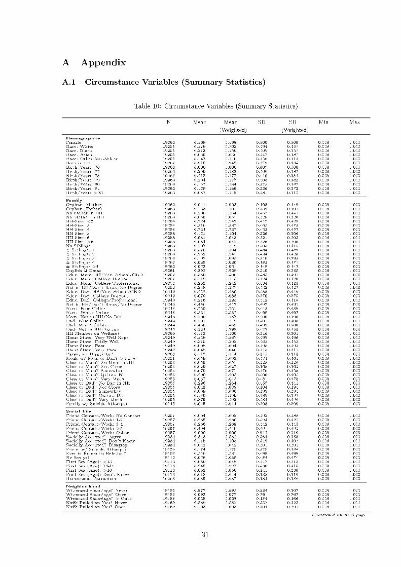
A Appendix
A.1 Circumstance Variables (Summary Statistics)
Table 10: Circumstance Variables (Summary Statistics)
N Mean Mean
(Weighted)
SD SD
(Weighted)
Min Max
DemographicsFemale 19263 0.509 0.498 0.500 0.500 0.000 1.000Race: White 19255 0.579 0.703 0.494 0.457 0.000 1.000Race: Black 19255 0.213 0.150 0.409 0.357 0.000 1.000Race: Asian 19255 0.065 0.036 0.247 0.187 0.000 1.000Race: Other Non-White 19255 0.143 0.110 0.350 0.313 0.000 1.000Born in US 19262 0.915 0.942 0.279 0.234 0.000 1.000Birth/Year: '76 19263 0.000 0.000 0.007 0.000 0.000 1.000Birth/Year: '77 19263 0.200 0.183 0.400 0.387 0.000 1.000Birth/Year: '78 19263 0.213 0.177 0.410 0.382 0.000 1.000Birth/Year: '79 19263 0.204 0.177 0.403 0.382 0.000 1.000Birth/Year: '80 19263 0.167 0.184 0.373 0.387 0.000 1.000Birth/Year: '81 19263 0.129 0.166 0.336 0.372 0.000 1.000Birth/Year: >'81 19263 0.087 0.112 0.281 0.315 0.000 1.000
FamilyOrphan (Mother) 19263 0.041 0.023 0.198 0.149 0.000 1.000Orphan (Father) 19263 0.133 0.101 0.339 0.301 0.000 1.000No Father in HH 19263 0.296 0.264 0.457 0.441 0.000 1.000No Mother in HH 19263 0.055 0.051 0.228 0.220 0.000 1.000HH-Size: <3 19258 0.224 0.242 0.417 0.429 0.000 1.000HH-Size: 3 19258 0.316 0.337 0.465 0.473 0.000 1.000HH-Size: 4 19258 0.234 0.232 0.423 0.422 0.000 1.000HH-Size: 5 19258 0.121 0.104 0.326 0.306 0.000 1.000HH-Size: 6 19258 0.051 0.043 0.221 0.203 0.000 1.000HH-Size: >6 19258 0.054 0.042 0.226 0.200 0.000 1.000No Siblings 19263 0.207 0.219 0.405 0.414 0.000 1.000# Siblings: 1 19263 0.376 0.394 0.484 0.489 0.000 1.000# Siblings: 2 19263 0.252 0.241 0.434 0.428 0.000 1.000# Siblings: 3 19263 0.108 0.095 0.310 0.293 0.000 1.000# Siblings: 4 19263 0.035 0.030 0.183 0.171 0.000 1.000# Siblings: >4 19263 0.023 0.021 0.149 0.142 0.000 1.000English @ Home 19261 0.892 0.929 0.310 0.258 0.000 1.000Educ. Mom: HS/Voc. School/GED 19252 0.380 0.406 0.485 0.491 0.000 1.000Educ. Mom: College Dropout 19252 0.119 0.115 0.324 0.320 0.000 1.000Educ. Mom: College/Professional 19252 0.252 0.242 0.434 0.428 0.000 1.000Not in HH/Don't Know/No Degree 19252 0.248 0.237 0.432 0.425 0.000 1.000Educ. Dad: HS/Voc. School/GED 19249 0.258 0.280 0.438 0.449 0.000 1.000Educ. Dad: College Dropout 19249 0.079 0.083 0.270 0.275 0.000 1.000Educ. Dad: College/Professional 19249 0.216 0.225 0.412 0.418 0.000 1.000Not in HH/Don't Know/No Degree 19249 0.446 0.412 0.497 0.492 0.000 1.000Mom: Blue Collar 19248 0.269 0.261 0.443 0.439 0.000 1.000Mom: White Collar 19248 0.531 0.552 0.499 0.497 0.000 1.000Mom: Not in HH/No Job 19248 0.200 0.187 0.400 0.390 0.000 1.000Dad: Blue Collar 19244 0.201 0.212 0.401 0.408 0.000 1.000Dad: White Collar 19244 0.465 0.489 0.499 0.500 0.000 1.000Dad: Not in HH/No Job 19244 0.334 0.299 0.472 0.458 0.000 1.000HH-Member on Welfare? 19260 0.113 0.100 0.316 0.301 0.000 1.000Home State: Very Well Kept 19249 0.539 0.567 0.499 0.496 0.000 1.000Home State: Fairly Well 19249 0.315 0.292 0.465 0.455 0.000 1.000Home State: Poor 19249 0.098 0.094 0.298 0.293 0.000 1.000Home State: Very Poor 19249 0.048 0.046 0.213 0.211 0.000 1.000Parent w/ Disability? 19263 0.112 0.114 0.315 0.318 0.000 1.000Meals w/ Mom or Dad? >4 d/w 19251 0.659 0.693 0.474 0.461 0.000 1.000Close to Mom? No Mom in HH 19256 0.055 0.051 0.228 0.220 0.000 1.000Close to Mom? Not Close 19256 0.029 0.027 0.168 0.162 0.000 1.000Close to Mom? Somewhat 19256 0.079 0.071 0.270 0.258 0.000 1.000Close to Mom? Quite a Bit 19256 0.200 0.205 0.400 0.404 0.000 1.000Close to Mom? Very Much 19256 0.637 0.645 0.481 0.478 0.000 1.000Close to Dad? No Dad in HH 19255 0.296 0.264 0.457 0.441 0.000 1.000Close to Dad? Not Close 19255 0.043 0.039 0.204 0.194 0.000 1.000Close to Dad? Somewhat 19255 0.099 0.096 0.299 0.294 0.000 1.000Close to Dad? Quite a Bit 19255 0.186 0.199 0.389 0.399 0.000 1.000Close to Dad? Very Much 19255 0.375 0.402 0.484 0.490 0.000 1.000Family w/ Suicide Attempt? 19145 0.045 0.044 0.208 0.206 0.000 1.000
Social LifeFriend Contact/Week: No Contact 19257 0.094 0.092 0.292 0.288 0.000 1.000Friend Contact/Week: 1-2 19257 0.235 0.230 0.424 0.421 0.000 1.000Friend Contact/Week: 3-4 19257 0.266 0.268 0.442 0.443 0.000 1.000Friend Contact/Week: >5 19257 0.404 0.410 0.491 0.492 0.000 1.000Friend Contact/Week: Other 19257 0.000 0.000 0.012 0.016 0.000 1.000Socially Accepted? Agree 19234 0.843 0.852 0.364 0.355 0.000 1.000Socially Accepted? Don't Know 19234 0.115 0.105 0.319 0.307 0.000 1.000Socially Accepted? Disagree 19234 0.042 0.042 0.201 0.201 0.000 1.000Friend w/ Suicide Attempt? 19136 0.174 0.179 0.379 0.384 0.000 1.000Ever in Romantic Relation? 19193 0.546 0.531 0.498 0.499 0.000 1.000No Sex yet 19113 0.626 0.659 0.484 0.474 0.000 1.000First Sex (Age): <13 19113 0.050 0.048 0.217 0.215 0.000 1.000First Sex (Age): 13-16 19113 0.245 0.223 0.430 0.416 0.000 1.000First Sex (Age): >16 19113 0.062 0.056 0.241 0.230 0.000 1.000First Sex (Age): Don't Know 19113 0.018 0.014 0.133 0.116 0.000 1.000Homosexual Attraction 19263 0.035 0.037 0.184 0.189 0.000 1.000
NeighborhoodWitnessed Shootings? Never 19155 0.872 0.895 0.334 0.307 0.000 1.000Witnessed Shootings? Once 19155 0.093 0.077 0.291 0.267 0.000 1.000Witnessed Shootings? > Once 19155 0.035 0.028 0.184 0.166 0.000 1.000Knife Pulled on You? Never 19160 0.869 0.882 0.337 0.322 0.000 1.000Knife Pulled on You? Once 19160 0.103 0.093 0.304 0.291 0.000 1.000
Continued on next page
31
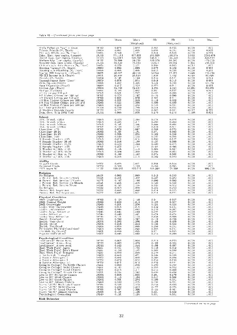
Table 10 Continued from previous page
N Mean Mean
(Weighted)
SD SD
(Weighted)
Min Max
Knife Pulled on You? > Once 19160 0.028 0.024 0.164 0.155 0.000 1.000Private Schools (%, Tract) 19059 0.097 0.088 0.095 0.091 0.000 0.84425+ w/o HS-Degree (%, Tract) 19096 0.284 0.271 0.144 0.140 0.000 0.874Educ. Exp. (per capita, County) 19153 674.154 677.025 159.929 156.375 2.542 2281.676Health Exp. (per capita, County) 19153 142.053 141.747 141.611 156.240 0.000 839.839Welfare Exp. (per capita, County) 19153 76.399 58.058 103.578 88.500 0.000 473.003Security Exp. (per capita, County) 19153 89.520 78.343 45.879 39.791 7.481 198.406Children w/o Both Parents (%, Tract) 19076 0.270 0.251 0.169 0.165 0.012 1.000Housing Vacancy (%, Tract) 19090 0.083 0.088 0.079 0.082 0.000 0.858Housing w/o Plumbing (%, Tract) 19088 0.008 0.008 0.015 0.016 0.000 0.297Median HH Income in k (Tract) 19075 30.887 30.006 13.399 12.558 4.999 125.053SD HH Income in k (Tract) 19075 25.898 25.519 7.836 7.932 6.916 66.828Poverty (%, Tract) 19094 0.145 0.144 0.123 0.121 0.000 0.864Unemployment Rate (Tract) 19079 0.076 0.075 0.048 0.048 0.000 0.658Pers./Sq.-km (Tract) 19098 1.807 1.388 3.424 3.016 0.000 69.172Race Dispersion (Tract) 19094 0.317 0.254 0.272 0.241 0.000 0.933Median Age (Tract) 19094 32.096 32.137 4.395 4.213 12.667 64.580Foreign % (Tract) 19096 0.103 0.065 0.161 0.117 0.000 0.869<1 Crime per 100 ppl 19263 0.691 0.792 0.462 0.406 0.000 1.0001-2 Violent Crimes per 100 ppl 19263 0.274 0.187 0.446 0.390 0.000 1.000>2 Violent Crimes per 100 ppl 19263 0.035 0.020 0.184 0.141 0.000 1.000<3 Non-Violent Crimes per 100 ppl 19263 0.225 0.248 0.418 0.432 0.000 1.0003-6 Non-Violent Crimes per 100 ppl 19263 0.522 0.500 0.500 0.500 0.000 1.000>6 Non-Violent Crimes per 100 ppl 19263 0.253 0.253 0.435 0.434 0.000 1.000Mail Vote pre-NVRA 19154 0.730 0.709 0.444 0.454 0.000 1.000% Working Outside County 19154 0.222 0.243 0.182 0.181 0.017 0.738Dem./Rep. % in 1992 Vote 19154 0.060 0.038 0.179 0.175 -0.408 0.624
SchoolDist. School: <2km 19263 0.353 0.346 0.478 0.476 0.000 1.000Dist. School: 2-5km 19263 0.328 0.311 0.469 0.463 0.000 1.000Dist. School: 5-10km 19263 0.185 0.206 0.388 0.404 0.000 1.000Dist. School: >10km 19263 0.134 0.137 0.340 0.344 0.000 1.000Class Size: <20 19263 0.079 0.082 0.269 0.275 0.000 1.000Class Size: 20-24 19263 0.165 0.191 0.371 0.393 0.000 1.000Class Size: 25-29 19263 0.308 0.295 0.462 0.456 0.000 1.000Class Size: >30 19263 0.449 0.433 0.497 0.495 0.000 1.000% Female Teacher: <25 19263 0.012 0.016 0.109 0.127 0.000 1.000% Female Teacher: 26-50 19263 0.256 0.199 0.437 0.399 0.000 1.000% Female Teacher: 51-75 19263 0.359 0.344 0.480 0.475 0.000 1.000% Female Teacher: >75 19263 0.373 0.441 0.484 0.496 0.000 1.000% Teacher w/ MA: < 25 19263 0.158 0.113 0.365 0.317 0.000 1.000% Teacher w/ MA: 26-50 19263 0.304 0.309 0.460 0.462 0.000 1.000% Teacher w/ MA: 51-75 19263 0.169 0.162 0.375 0.368 0.000 1.000% Teacher w/ MA: >75 19263 0.368 0.416 0.482 0.493 0.000 1.000
AbilitySkipped Grade 19252 0.028 0.021 0.164 0.143 0.000 1.000Repeated Grade 19254 0.204 0.194 0.403 0.395 0.000 1.000PVT Score W1 14133 130.343 135.715 161.384 171.509 9.000 996.000
ReligionNo Religion 16525 0.063 0.069 0.242 0.253 0.000 1.000# Parent: Rel. Service 1/Week 16525 0.385 0.367 0.487 0.482 0.000 1.000# Parent: Rel. Service 1/Month 16525 0.187 0.190 0.390 0.393 0.000 1.000# Parent: Rel. Service <1/Month 16525 0.238 0.238 0.426 0.426 0.000 1.000# Parent: Rel. Service Never 16525 0.127 0.136 0.333 0.342 0.000 1.000No Religion 16522 0.063 0.069 0.242 0.253 0.000 1.000Parent: Rel. Important 16522 0.889 0.880 0.314 0.325 0.000 1.000Parent: Rel. Not Important 16522 0.048 0.051 0.214 0.221 0.000 1.000
Physical ConditionBMI: Underweight 19263 0.134 0.150 0.341 0.357 0.000 1.000BMI: Normal Weight 19263 0.630 0.614 0.483 0.487 0.000 1.000BMI: Overweight 19263 0.235 0.236 0.424 0.425 0.000 1.000Looks: Very Unattractive 19246 0.018 0.018 0.132 0.131 0.000 1.000Looks: Unattractive 19246 0.046 0.045 0.210 0.207 0.000 1.000Looks: Avrg. Attractive 19246 0.446 0.444 0.497 0.497 0.000 1.000Looks: Attractive 19246 0.340 0.341 0.474 0.474 0.000 1.000Looks: Very Attractive 19246 0.151 0.153 0.358 0.360 0.000 1.000Health: Excellent 19258 0.280 0.282 0.449 0.450 0.000 1.000Health: Very Good 19258 0.393 0.396 0.488 0.489 0.000 1.000Health: Good 19258 0.256 0.254 0.436 0.435 0.000 1.000Health: Not Good 19258 0.070 0.068 0.256 0.251 0.000 1.000Permanent Physical Condition? 19253 0.028 0.023 0.165 0.151 0.000 1.000Use Mobility Device? 19255 0.030 0.028 0.171 0.165 0.000 1.000Physical Diculties? 19257 0.048 0.042 0.213 0.200 0.000 1.000
Psychological ConditionIntelligence? Below Avrg. 19244 0.063 0.068 0.243 0.252 0.000 1.000Intelligence? About Avrg. 19244 0.394 0.378 0.489 0.485 0.000 1.000Intelligence? Above Avrg. 19244 0.543 0.554 0.498 0.497 0.000 1.000Hard Work Pays? Agree 19237 0.737 0.733 0.440 0.442 0.000 1.000Hard Work Pays? Don't Know 19237 0.184 0.187 0.388 0.390 0.000 1.000Hard Work Pays? Disagree 19237 0.079 0.080 0.270 0.271 0.000 1.000# No Suicidal Thoughts 19259 0.869 0.871 0.338 0.336 0.000 1.000# Suicide Attempts: 0 19259 0.092 0.092 0.289 0.288 0.000 1.000# Suicide Attempts: 1 19259 0.024 0.025 0.153 0.156 0.000 1.000# Suicide Attempts: >1 19259 0.015 0.013 0.123 0.114 0.000 1.000Going to College? No/Little Chance 19211 0.099 0.099 0.299 0.298 0.000 1.000Going to College? 50:50 Chance 19211 0.147 0.145 0.355 0.352 0.000 1.000Going to College? Good Chance 19211 0.218 0.211 0.413 0.408 0.000 1.000Going to College? Almost Certain 19211 0.536 0.545 0.499 0.498 0.000 1.000Live to 35? No/Little Chance 19204 0.038 0.033 0.191 0.179 0.000 1.000Live to 35? 50:50 Chance 19204 0.113 0.104 0.317 0.306 0.000 1.000Live to 35? Good Chance 19204 0.305 0.284 0.460 0.451 0.000 1.000Live to 35? Almost Certain 19204 0.544 0.578 0.498 0.494 0.000 1.000Marry 'til 25? No/Little Chance 19206 0.233 0.223 0.423 0.416 0.000 1.000Marry 'til 25? 50:50 Chance 19206 0.349 0.344 0.477 0.475 0.000 1.000Marry 'til 25? Good Chance 19206 0.292 0.306 0.455 0.461 0.000 1.000Marry 'til 25? Almost Certain 19206 0.125 0.126 0.331 0.332 0.000 1.000Psychological Counseling 19249 0.125 0.125 0.331 0.331 0.000 1.000
Risk Behavior
Continued on next page
32
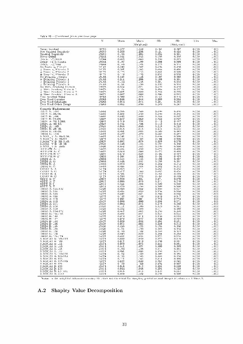
Table 10 Continued from previous page
N Mean Mean
(Weighted)
SD SD
(Weighted)
Min Max
Never Smoked 19250 0.577 0.559 0.494 0.497 0.000 1.000Not Smoked Regularly 19250 0.230 0.236 0.421 0.425 0.000 1.000Smoked Regularly 19250 0.193 0.205 0.395 0.404 0.000 1.000Never Drink 19244 0.541 0.543 0.498 0.498 0.000 1.000Drink: 1-7/Week 19244 0.093 0.089 0.290 0.285 0.000 1.000Drink: <1-3/Month 19244 0.197 0.199 0.398 0.399 0.000 1.000Drink: 1-2/Year 19244 0.169 0.168 0.375 0.374 0.000 1.000No Smoking Friends 19121 0.549 0.547 0.498 0.498 0.000 1.000# Smoking Friends: 1 19121 0.205 0.205 0.403 0.404 0.000 1.000# Smoking Friends: 2 19121 0.128 0.125 0.334 0.330 0.000 1.000# Smoking Friends: 3 19121 0.119 0.123 0.324 0.328 0.000 1.000No Drinking Friends 19103 0.445 0.456 0.497 0.498 0.000 1.000# Drinking Friends: 1 19103 0.211 0.206 0.408 0.404 0.000 1.000# Drinking Friends: 2 19103 0.154 0.148 0.361 0.355 0.000 1.000# Drinking Friends: 3 19103 0.191 0.190 0.393 0.393 0.000 1.000No Weed Smoking Friends 19078 0.652 0.671 0.476 0.470 0.000 1.000# Weed Smoking Friends: 1 19078 0.156 0.150 0.363 0.357 0.000 1.000# Weed Smoking Friends: 2 19078 0.095 0.090 0.293 0.286 0.000 1.000# Weed Smoking Friends: 3 19078 0.097 0.089 0.296 0.285 0.000 1.000Ever Smoked Weed 19263 0.290 0.274 0.454 0.446 0.000 1.000Ever Used Cocaine 19263 0.046 0.044 0.209 0.205 0.000 1.000Ever Used Inhalants 19263 0.074 0.075 0.261 0.263 0.000 1.000Ever Used Other Drugs 19263 0.092 0.090 0.289 0.287 0.000 1.000
Genetic EndowmentDAT1 A: >9R 13802 0.598 0.580 0.490 0.494 0.000 1.000DAT1 A: 3R-9R 13802 0.402 0.420 0.490 0.494 0.000 1.000DAT1 B: >9R 13802 0.943 0.940 0.233 0.237 0.000 1.000DAT1 B: 7R-9R 13802 0.057 0.060 0.233 0.237 0.000 1.000DRD4 A: 2R-3.39R 13815 0.219 0.224 0.413 0.417 0.000 1.000DRD4 A: 4R-6R 13815 0.731 0.726 0.443 0.446 0.000 1.000DRD4 A: >6R 13815 0.050 0.050 0.218 0.218 0.000 1.000DRD4 B: 2R-3R 13815 0.018 0.018 0.134 0.133 0.000 1.000DRD4 B: 4R-6R 13815 0.605 0.603 0.489 0.489 0.000 1.000DRD4 B: >6R 13815 0.377 0.379 0.485 0.485 0.000 1.000MAOA_V A: 2R-3.5R 13825 0.541 0.516 0.498 0.500 0.000 1.000MAOA_V A: 4R-5R 13825 0.459 0.484 0.498 0.500 0.000 1.000MAOA_V B: 2R-3.5R 13825 0.092 0.079 0.289 0.270 0.000 1.000MAOA_V B: 4R-5R 13825 0.446 0.435 0.497 0.496 0.000 1.000MAOA_V B: Male 13825 0.462 0.485 0.499 0.500 0.000 1.000HTTLPR A: L' 13838 0.336 0.320 0.472 0.466 0.000 1.000HTTLPR A: S' 13838 0.664 0.680 0.472 0.466 0.000 1.000HTTLPR B: L' 13838 0.619 0.634 0.486 0.482 0.000 1.000HTTLPR B: S' 13838 0.381 0.366 0.486 0.482 0.000 1.000DRD2 A: A 13693 0.452 0.443 0.498 0.497 0.000 1.000DRD2 A: G 13693 0.548 0.557 0.498 0.497 0.000 1.000DRD2 B: A 13693 0.074 0.062 0.262 0.242 0.000 1.000DRD2 B: G 13693 0.926 0.938 0.262 0.242 0.000 1.000COMT A: A 13174 0.683 0.711 0.465 0.454 0.000 1.000COMT A: G 13174 0.317 0.289 0.465 0.454 0.000 1.000COMT B: A 13174 0.206 0.227 0.404 0.419 0.000 1.000COMT B: G 13174 0.794 0.773 0.404 0.419 0.000 1.0005HTT A: C 12872 0.920 0.921 0.271 0.270 0.000 1.0005HTT A: T 12872 0.080 0.079 0.271 0.270 0.000 1.0005HTT B: C 12872 0.521 0.504 0.500 0.500 0.000 1.0005HTT B: T 12872 0.479 0.496 0.500 0.500 0.000 1.000DRD5 A: 124-132 13525 0.029 0.022 0.169 0.147 0.000 1.000DRD5 A: 134 13525 0.026 0.029 0.158 0.168 0.000 1.000DRD5 A: 136 13525 0.042 0.041 0.200 0.198 0.000 1.000DRD5 A: 138 13525 0.133 0.140 0.340 0.347 0.000 1.000DRD5 A: 140 13525 0.081 0.081 0.273 0.273 0.000 1.000DRD5 A: 142 13525 0.090 0.080 0.286 0.271 0.000 1.000DRD5 A: 144 13525 0.084 0.073 0.278 0.260 0.000 1.000DRD5 A: 146 13525 0.115 0.109 0.319 0.311 0.000 1.000DRD5 A: 148 13525 0.332 0.360 0.471 0.480 0.000 1.000DRD5 A: 150-172 13525 0.067 0.065 0.250 0.246 0.000 1.000DRD5 B: 126-138 13525 0.022 0.021 0.145 0.144 0.000 1.000DRD5 B: 140 13525 0.014 0.014 0.120 0.116 0.000 1.000DRD5 B: 142 13525 0.029 0.027 0.168 0.162 0.000 1.000DRD5 B: 144 13525 0.039 0.034 0.194 0.181 0.000 1.000DRD5 B: 146 13525 0.072 0.063 0.258 0.243 0.000 1.000DRD5 B: 148 13525 0.429 0.433 0.495 0.496 0.000 1.000DRD5 B: 150 13525 0.181 0.190 0.385 0.392 0.000 1.000DRD5 B: 152 13525 0.139 0.142 0.346 0.349 0.000 1.000DRD5 B: 154 13525 0.043 0.050 0.204 0.218 0.000 1.000DRD5 B: 156-174 13525 0.032 0.026 0.175 0.159 0.000 1.000MAOCA1 A: 101-113 13574 0.030 0.020 0.172 0.140 0.000 1.000MAOCA1 A: 109 13574 0.015 0.010 0.120 0.101 0.000 1.000MAOCA1 A: 111 13574 0.070 0.073 0.255 0.261 0.000 1.000MAOCA1 A: 113 13574 0.515 0.537 0.500 0.499 0.000 1.000MAOCA1 A: 115 13574 0.164 0.156 0.371 0.363 0.000 1.000MAOCA1 A: 117 13574 0.025 0.023 0.156 0.149 0.000 1.000MAOCA1 A: 119-131 13574 0.182 0.180 0.386 0.384 0.000 1.000MAOCA1 B: 103-113 13574 0.139 0.143 0.346 0.350 0.000 1.000MAOCA1 B: 115 13574 0.111 0.105 0.314 0.306 0.000 1.000MAOCA1 B: 117-119 13574 0.043 0.039 0.204 0.195 0.000 1.000MAOCA1 B: 121 13574 0.170 0.160 0.376 0.367 0.000 1.000MAOCA1 B: 123 13574 0.016 0.012 0.124 0.110 0.000 1.000MAOCA1 B: 125 13574 0.044 0.046 0.204 0.210 0.000 1.000MAOCA1 B: 127-131 13574 0.018 0.013 0.133 0.113 0.000 1.000MAOCA1 B: Male 13574 0.460 0.482 0.498 0.500 0.000 1.000
Note: In the weighted columns summary statistics are corrected for sampling procedure and sample attrition until Wave 3.
A.2 Shapley Value Decomposition
33
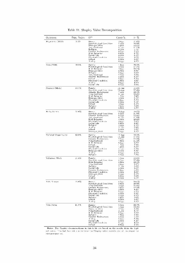
Table 11: Shapley Value Decomposition
Outcome Diss. Index Ωm Contrib. in %
Registered (2000) 9.5% Family 2.0pp 21.0%Psychological Condition 1.5pp 16.0%Demographics 1.2pp 12.5%Neighborhood 1.1pp 11.1%Religion 0.7pp 7.7%Genetic Endowment 0.7pp 7.3%Risk Behavior 0.6pp 6.7%Social Life 0.6pp 6.3%Physical Condition 0.5pp 4.8%School 0.4pp 3.8%Ability 0.3pp 2.8%
Vote (2000) 19.8% Family 4.0pp 20.3%Psychological Condition 3.5pp 17.7%Risk Behavior 2.0pp 10.1%Demographics 1.9pp 9.6%Religion 1.9pp 9.6%Neighborhood 1.7pp 8.8%Genetic Endowment 1.2pp 6.1%School 1.0pp 5.1%Physical Condition 1.0pp 4.9%Ability 0.8pp 4.1%Social Life 0.7pp 3.6%
Contact Ocial 59.7% Family 13.7pp 23.0%Psychological Condition 10.4pp 17.4%Genetic Endowment 7.5pp 12.5%Neighborhood 6.1pp 10.2%Risk Behavior 4.7pp 7.9%Demographics 3.5pp 5.9%Physical Condition 3.4pp 5.7%Social Life 3.2pp 5.4%School 3.0pp 5.1%Religion 2.6pp 4.3%Ability 1.6pp 2.6%
Rally/March 55.4% Family 13.0pp 23.5%Psychological Condition 8.3pp 14.9%Genetic Endowment 6.7pp 12.2%Neighborhood 6.1pp 11.0%Risk Behavior 5.9pp 10.6%Physical Condition 3.8pp 7.0%Social Life 3.8pp 6.9%Religion 2.9pp 5.3%Ability 2.1pp 3.9%School 1.5pp 2.6%Demographics 1.3pp 2.3%
Political Organization 63.0% Family 11.5pp 18.3%Psychological Condition 11.2pp 17.8%Genetic Endowment 7.7pp 12.3%Neighborhood 7.0pp 11.2%Risk Behavior 6.2pp 9.8%School 4.4pp 7.0%Social Life 4.2pp 6.6%Physical Condition 4.1pp 6.5%Demographics 3.7pp 5.9%Ability 1.5pp 2.4%Religion 1.4pp 2.2%
Volunteer Work 24.0% Family 4.7pp 19.8%Psychological Condition 4.2pp 17.4%Risk Behavior 3.0pp 12.5%Neighborhood 2.2pp 9.1%Religion 2.1pp 8.8%Social Life 1.9pp 8.0%Genetic Endowment 1.4pp 6.0%Physical Condition 1.4pp 6.0%Demographics 1.3pp 5.5%School 0.9pp 3.6%Ability 0.8pp 3.4%
Vote Always 22.4% Family 4.2pp 18.6%Psychological Condition 3.6pp 16.0%Neighborhood 3.3pp 14.9%Genetic Endowment 2.9pp 12.8%Demographics 2.0pp 8.8%Risk Behavior 1.5pp 6.7%Physical Condition 1.3pp 5.8%Social Life 1.3pp 5.6%Religion 1.0pp 4.6%School 0.9pp 3.8%Ability 0.5pp 2.3%
Vote Never 24.5% Family 5.4pp 22.2%Psychological Condition 4.5pp 18.3%Demographics 2.2pp 9.1%Neighborhood 2.1pp 8.7%Risk Behavior 1.9pp 7.9%Religion 1.9pp 7.8%Genetic Endowment 1.8pp 7.5%Ability 1.3pp 5.5%Social Life 1.3pp 5.1%Physical Condition 1.1pp 4.5%School 0.9pp 3.5%
Note: The Shapley decompositions in this table are based on the results from the logit
estimator. The last two columns indicate the Shapley value contribution of the respective
circumstance set.
34
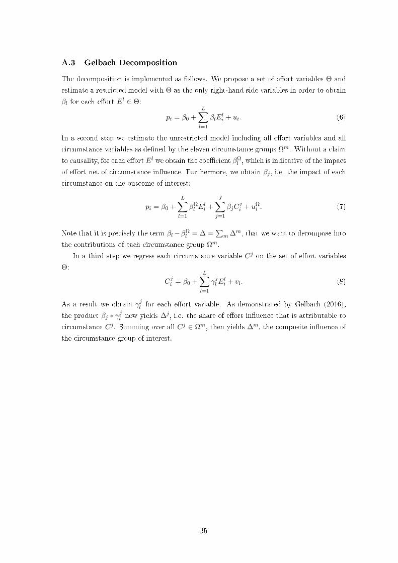
A.3 Gelbach Decomposition
The decomposition is implemented as follows. We propose a set of eort variables Θ and
estimate a restricted model with Θ as the only right-hand side variables in order to obtain
βl for each eort El ∈ Θ:
pi = β0 +L∑l=1
βlEli + ui. (6)
In a second step we estimate the unrestricted model including all eort variables and all
circumstance variables as dened by the eleven circumstance groups Ωm. Without a claim
to causality, for each eort El we obtain the coecient βΩl , which is indicative of the impact
of eort net of circumstance inuence. Furthermore, we obtain βj , i.e. the impact of each
circumstance on the outcome of interest:
pi = β0 +
L∑l=1
βΩl E
li +
J∑j=1
βjCji + uΩ
i . (7)
Note that it is precisely the term βl−βΩl = ∆ =
∑m ∆m, that we want to decompose into
the contributions of each circumstance group Ωm.
In a third step we regress each circumstance variable Cj on the set of eort variables
Θ:
Cji = β0 +L∑l=1
γjl Eli + vi. (8)
As a result we obtain γjl for each eort variable. As demonstrated by Gelbach (2016),
the product βj ∗ γjl now yields ∆j , i.e. the share of eort inuence that is attributable to
circumstance Cj . Summing over all Cj ∈ Ωm, then yields ∆m, the composite inuence of
the circumstance group of interest.
35