Best-first Word-lattice Parsing:

Techniques for integrated syntactic language modeling

by

Keith B. Hall

B. S., Mary Washington College, 1993

Sc. M., Brown University, 2001

A dissertation submitted in partial fulfillment of the

requirements for the Degree of Doctor of Philosophy

in the Department of Computer Science at Brown University

Providence, Rhode Island

May 2005

c© Copyright 2005 by Keith B. Hall

This dissertation by Keith B. Hall is accepted in its present form by

the Department of Computer Science as satisfying the dissertation requirement

for the degree of Doctor of Philosophy.

DateMark Johnson, Director

Recommended to the Graduate Council

DateEugene Charniak, Reader

(Brown University)

DateFrederick Jelinek, Reader

(Johns Hopkins University)

Approved by the Graduate Council

DateKaren Newman

Dean of the Graduate School

iii

Abstract of “Best-first Word-lattice Parsing:

Techniques for integrated syntactic language modeling” by Keith B. Hall, Ph.D., Brown University,

May 2005.

This thesis explores a language modeling technique based on statistical parsing. Previous re-

search that exploits syntactic structure for modeling language has shown improved accuracy over

the standard trigram models. Unlike previous techniques, our parsing model performs syntactic

analysis on sets of hypothesized word-strings simultaneously; these sets are encoded as weighted fi-

nite state automata word-lattices. We present a best-first word-lattice chart parsing algorithm which

combines the search for good parses with the search for good strings in the word-lattice. We de-

scribe how the word-lattice parser is combined with the Charniak language model, a sophisticated

syntactic language model, in order to provide an efficient syntactic language model. We present

results for this model on a standard set of speech recognition word-lattices. Finally, we examine

variations of the word-lattice parser in order to increase performance as well as accuracy.

Preface

The computational efforts during the past 30 years and, more importantly, the introduction of struc-

tured statistical models introduced over the last 10 years have resulted in a general framework for

approaching Natural Language Processing (NLP). In particular, we note the results from lexicalized

statistical parsers that have been used in discovering syntactic structure as well as predicting strings

of words (Charniak, 2001; Roark, 2001a; Collins, 2003). Recently, there have been positive results

incorporating syntactic analysis into language modeling (i.e., predicting strings of words) which is

an integral component of many Natural Language Processing models. The focus of this thesis is to

explore the integration of statistical parsing techniques into language modeling.

Until recently, it has been nearly impossible to design a language model that performs better than

the n-gram model. While we don’t suggest that an n-gram model is a realistic model for language

generation (though a 7-gram generates some realistic sentences), we recognize that language models

are used to select from ambiguous strings. In speech recognition, the n-gram has been relatively

successful in disambiguating the output of an acoustic recognizer. This is likely due to the relatively

local ambiguity present in the output generated by acoustic recognizers. In other NLP domains, such

as machine translation, non-local ambiguity is a more significant problem suggesting that n-gram

models may not be as powerful as when used for speech recognition.

Recent results with syntactically based language modeling techniques show that there is some-

thing to be gained by considering the syntactic structure when predicting word strings (Charniak,

2001; Xu et al., 2002). We note that much work has been done on improving the standard n-gram

modeling paradigm (see Goodman (2001)) and that the most commonly used n-gram - the trigram

- is not the most powerful n-gram model. However, many of the more successful techniques focus

on selecting words to be considered in the prediction context (skip models), something that comes

v

naturally from syntactic language models.

A small example may help elucidate the aspects of language modeling that are readily identified

by syntactic techniques. Consider a speech recognition system that posits the following two strings

for an utterance with relatively equal likelihood:

1. I put the file in the drawer

2. I put the file and the drawer

Semantic analysis is likely to help resolve the ambiguity between these two hypotheses. Under the

standard trigram model we assign probability to the ambiguous word as follows.

1. P (and|the file)

2. P (in|the file)

vi

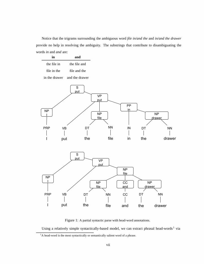
Notice that the trigrams surrounding the ambiguous word file in/and the and in/and the drawer

provide no help in resolving the ambiguity. The substrings that contribute to disambiguating the

words in and and are:

in and

the file in the file and

file in the file and the

in the drawer and the drawer

NPI

VPput

NPfile

PPin

Sput

PRP VB DT NN IN DT NN

NPdrawer

I put the file in the drawer

NPI

VPput

NPfile

CCand

Sput

PRP VB DT NN CC DT NN

NPdrawer

I put the file and the drawer

NPfile

Figure 1: A partial syntactic parse with head-word annotations.

Using a relatively simple syntactically-based model, we can extract phrasal head-words1 via

1A head-word is the most syntactically or semantically salient word of a phrase.

vii

structured analysis. For example, under a simplified version of the Structured Language Model

(Chelba and Jelinek, 2000), these are the predictive probabilities for the ambiguous words given the

head-word annotated parses in Figure 1:

1. P (and|put file)

2. P (in|put)

When we predict the word drawer we will use the probabilities for:

1. P (drawer|put in)

2. P (drawer|file put)

Under the trigram model, we consider local contexts of the surface strings, but under a syntactic

model we consider local contexts of the syntactic structure. In this example, we believe the structure

will reveal that it is more likely to use the word in than the word and.

The above model makes use of the syntactic structure solely to obtain lexical head-words. How-

ever, there is ambiguity in identifying syntactic structures, so it is probably useful to consider the

likelihood of particular parses given a probabilistic grammar. In this thesis we work with a language

model based on probabilistic lexicalized parsing, which defines a unified model over lexical depen-

dencies, such as those described above, along with syntactic dependencies defined by a grammar.

Although n-gram models are far more efficient in processing ambiguous analyses, the poten-

tial modeling improvement from syntactically-based models instigates the exploration of efficient

syntactic language modeling. Much work has been applied to exploring high-accuracy syntactic

parsing models as well as lower accuracy but very fast string parsing techniques (Abney, 1996). In

this work, we aim to explore techniques to efficiently and accurately parse word-lattices (a compact

representation of the ambiguous alternatives generated during speech recognition, machine transla-

tion, and other NLP tasks). We hope that the algorithms and analysis presented in this thesis provide

insight into the task of word-lattice parsing as well as framework for future work on syntactic lan-

guage modeling.

viii

Acknowledgments

I would like to thank Mark Johnson for providing an excellent environment for research. Mark

gave me the flexibility I needed to explore a variety of ideas, while also directing me towards

intellectually stimulating research problems. It has been a pleasure working with Mark. I would

also like to thank Eugene Charniak for introducing me to research in Natural Language Processing,

teaching me the necessary background, and providing a pleasant, collegial atmosphere to discuss

research in general. Fred Jelinek has been an invaluable member of my thesis committee, providing

me with insightful comments and inspiring commentary.

Discussions with Brian Roark, Ciprian Chelba, and Bill Byrne have been a tremendous help.

The Brown Laboratory for Linguistic Information Processing (BLLIP) that Eugene and Mark

have created is a wonderful place to work. I would like to thank all the members of the BLLIP

group from the past six years, but especially Brian Roark, Massi Ciaramita, Heidi Fox, Gideon

Mann, Sharon Caraballo, Don Blaheta, Sharon Goldwater, and Yasemin Altun. Their comments

and criticisms have helped develop my research.

There are a number of fellow graduate students in the Department of Computer Science at

Brown that I would like to thank. Don Carney for reminding me that not everybody is as interested

in parsing as am I. David Gondek for providing the simple answers for problems that I had let

intimidate me. Sam Heath, Joel Young, Srikanta Tirthapura, and Stuart Andrews for enjoyable

intellectual and non-intellectual conversation.

Amy Greenwald, with whom I worked with for a year exploring Computational Game Theory,

provided the support and motivation necessary for me to explore the research I find interesting. She

taught me that research can be fun. Amy is a wonderful person to work with.

Thanks to Ernie Ackermann and Judith Parker, my undergraduate advisors, who inspired my

ix

interests in both computer science and linguistics.

I would like to thank Andrea Wesol for putting up with the last four years of me in Graduate

School and reading and editing this thesis, which is as far away from her area of interest as possible.

Andrea, Hoover, and Jasper provided the companionship that got me through those lonely days and

nights in front of the computer.

And finally, I would like to thank my parents, who encouraged me to explore the ideas I find

interesting and provided the moral support necessary to pursue them.

x

Contents

List of Tables xiv

List of Figures xvi

1 Introduction 1

1.1 Representing Ambiguity: Word Lattices . . . . . . . . . . . . . . . . . . . . . . . 4

1.2 Language Modeling . . . . . . . . . . . . . . . . . . . . . . . . . . . . . . . . . . 5

1.3 Parsing and Language Modeling . . . . . . . . . . . . . . . . . . . . . . . . . . . 6

1.3.1 N -best string rescoring . . . . . . . . . . . . . . . . . . . . . . . . . . . . 6

1.3.2 Lattice Parsing . . . . . . . . . . . . . . . . . . . . . . . . . . . . . . . . 8

1.3.3 Structure of this Thesis . . . . . . . . . . . . . . . . . . . . . . . . . . . . 10

2 Background 11

2.1 Word-Lattices . . . . . . . . . . . . . . . . . . . . . . . . . . . . . . . . . . . . . 11

2.1.1 Raw Word-lattice Format . . . . . . . . . . . . . . . . . . . . . . . . . . . 12

2.1.2 Finite State Machines . . . . . . . . . . . . . . . . . . . . . . . . . . . . . 13

2.2 Probabilistic Context Free Grammars . . . . . . . . . . . . . . . . . . . . . . . . 19

2.2.1 Context Free Grammar . . . . . . . . . . . . . . . . . . . . . . . . . . . . 19

2.2.2 Probabilities and Context Free Grammars . . . . . . . . . . . . . . . . . . 20

2.2.3 Estimating PCFG Probabilities . . . . . . . . . . . . . . . . . . . . . . . . 22

2.2.4 Binarization . . . . . . . . . . . . . . . . . . . . . . . . . . . . . . . . . . 23

2.2.5 Markovization . . . . . . . . . . . . . . . . . . . . . . . . . . . . . . . . 26

2.3 Efficient Probabilistic Chart Parsing . . . . . . . . . . . . . . . . . . . . . . . . . 28

xi

2.3.1 Chart Parsing . . . . . . . . . . . . . . . . . . . . . . . . . . . . . . . . . 29

2.3.2 Best-first Chart Parsing . . . . . . . . . . . . . . . . . . . . . . . . . . . . 32

2.3.3 Using Binarized Grammars . . . . . . . . . . . . . . . . . . . . . . . . . . 37

2.3.4 A∗ Parsing and Coarse-to-fine Processing . . . . . . . . . . . . . . . . . . 38

3 Word-lattice Parsing 40

3.1 Previous Work . . . . . . . . . . . . . . . . . . . . . . . . . . . . . . . . . . . . . 40

3.2 Parsing over Word-lattices . . . . . . . . . . . . . . . . . . . . . . . . . . . . . . 42

3.2.1 Linear Spans . . . . . . . . . . . . . . . . . . . . . . . . . . . . . . . . . 42

3.2.2 Semantics of Parse Chart Edges . . . . . . . . . . . . . . . . . . . . . . . 44

3.3 Best-first Bottom-up Lattice Parsing . . . . . . . . . . . . . . . . . . . . . . . . . 46

3.3.1 Components of the Figure of Merit . . . . . . . . . . . . . . . . . . . . . 50

3.4 PCFG Figure of Merit . . . . . . . . . . . . . . . . . . . . . . . . . . . . . . . . . 51

3.4.1 Computing Viterbi Inside Probabilities . . . . . . . . . . . . . . . . . . . 52

3.4.2 Linear Outside Model . . . . . . . . . . . . . . . . . . . . . . . . . . . . 55

3.4.3 Boundary Models . . . . . . . . . . . . . . . . . . . . . . . . . . . . . . . 58

3.4.4 PCFG FOM . . . . . . . . . . . . . . . . . . . . . . . . . . . . . . . . . . 59

3.5 Inside-Outside Pruning for Word-lattice Charts . . . . . . . . . . . . . . . . . . . 60

4 Syntactic Language Modeling 63

4.1 Coarse-to-fine Chart Parsing . . . . . . . . . . . . . . . . . . . . . . . . . . . . . 64

4.1.1 Second-stage Memory Constraints . . . . . . . . . . . . . . . . . . . . . 67

5 Speech Recognition Experiments 68

5.1 Evaluation Metrics . . . . . . . . . . . . . . . . . . . . . . . . . . . . . . . . . . 69

5.1.1 Word Error Rate . . . . . . . . . . . . . . . . . . . . . . . . . . . . . . . 69

5.1.2 Oracle Word Error Rate . . . . . . . . . . . . . . . . . . . . . . . . . . . 69

5.2 Speech Data . . . . . . . . . . . . . . . . . . . . . . . . . . . . . . . . . . . . . . 71

5.3 Model Training . . . . . . . . . . . . . . . . . . . . . . . . . . . . . . . . . . . . 72

5.3.1 Estimating Preterminal Probabilities . . . . . . . . . . . . . . . . . . . . . 73

5.3.2 Training The Charniak Parser . . . . . . . . . . . . . . . . . . . . . . . . 74

xii

5.4 Experimental Setup . . . . . . . . . . . . . . . . . . . . . . . . . . . . . . . . . . 75

5.5 Results . . . . . . . . . . . . . . . . . . . . . . . . . . . . . . . . . . . . . . . . . 76

5.5.1 Generating local-trees . . . . . . . . . . . . . . . . . . . . . . . . . . . . 77

5.5.2 n-best Strings . . . . . . . . . . . . . . . . . . . . . . . . . . . . . . . . . 77

5.5.3 n-best Lattices . . . . . . . . . . . . . . . . . . . . . . . . . . . . . . . . 78

5.5.4 Acoustic Lattices . . . . . . . . . . . . . . . . . . . . . . . . . . . . . . . 80

5.5.5 Applicability of Syntactic Models . . . . . . . . . . . . . . . . . . . . . . 81

5.5.6 Summary and Discussion . . . . . . . . . . . . . . . . . . . . . . . . . . . 81

6 Alternate Grammar Models 83

6.1 Parent Annotated PCFG . . . . . . . . . . . . . . . . . . . . . . . . . . . . . . . 83

6.1.1 Experimental Results . . . . . . . . . . . . . . . . . . . . . . . . . . . . . 84

6.2 Lexicalized PCFG . . . . . . . . . . . . . . . . . . . . . . . . . . . . . . . . . . . 85

6.2.1 Finding Head-words . . . . . . . . . . . . . . . . . . . . . . . . . . . . . 86

6.2.2 Lexicalized PCFG Components . . . . . . . . . . . . . . . . . . . . . . . 87

6.2.3 Lexicalized Figure of Merit . . . . . . . . . . . . . . . . . . . . . . . . . 89

6.2.4 Estimating Model Parameters . . . . . . . . . . . . . . . . . . . . . . . . 91

6.2.5 Experimental Results . . . . . . . . . . . . . . . . . . . . . . . . . . . . . 92

7 Attention Shifting 94

7.1 Attention Shifting Algorithm . . . . . . . . . . . . . . . . . . . . . . . . . . . . . 94

7.2 Experiments . . . . . . . . . . . . . . . . . . . . . . . . . . . . . . . . . . . . . . 96

7.3 Summary . . . . . . . . . . . . . . . . . . . . . . . . . . . . . . . . . . . . . . . 97

8 Conclusion 99

8.1 Future Directions . . . . . . . . . . . . . . . . . . . . . . . . . . . . . . . . . . . 100

8.2 Summary . . . . . . . . . . . . . . . . . . . . . . . . . . . . . . . . . . . . . . . 101

Parts of this thesis have previously been published as (Hall and Johnson, 2003) and (Hall and

Johnson, 2004).

xiii

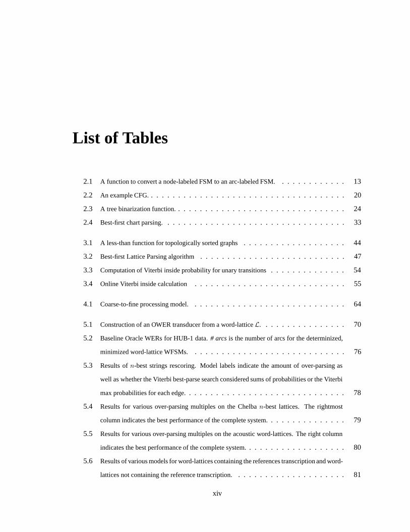
List of Tables

2.1 A function to convert a node-labeled FSM to an arc-labeled FSM. . . . . . . . . . . . . 13

2.2 An example CFG. . . . . . . . . . . . . . . . . . . . . . . . . . . . . . . . . . . . . 20

2.3 A tree binarization function. . . . . . . . . . . . . . . . . . . . . . . . . . . . . . . . 24

2.4 Best-first chart parsing. . . . . . . . . . . . . . . . . . . . . . . . . . . . . . . . . . 33

3.1 A less-than function for topologically sorted graphs . . . . . . . . . . . . . . . . . . . 44

3.2 Best-first Lattice Parsing algorithm . . . . . . . . . . . . . . . . . . . . . . . . . . . 47

3.3 Computation of Viterbi inside probability for unary transitions . . . . . . . . . . . . . . 54

3.4 Online Viterbi inside calculation . . . . . . . . . . . . . . . . . . . . . . . . . . . . 55

4.1 Coarse-to-fine processing model. . . . . . . . . . . . . . . . . . . . . . . . . . . . . 64

5.1 Construction of an OWER transducer from a word-lattice L. . . . . . . . . . . . . . . . 70

5.2 Baseline Oracle WERs for HUB-1 data. # arcs is the number of arcs for the determinized,

minimized word-lattice WFSMs. . . . . . . . . . . . . . . . . . . . . . . . . . . . . 76

5.3 Results of n-best strings rescoring. Model labels indicate the amount of over-parsing as

well as whether the Viterbi best-parse search considered sums of probabilities or the Viterbi

max probabilities for each edge. . . . . . . . . . . . . . . . . . . . . . . . . . . . . . 78

5.4 Results for various over-parsing multiples on the Chelba n-best lattices. The rightmost

column indicates the best performance of the complete system. . . . . . . . . . . . . . . 79

5.5 Results for various over-parsing multiples on the acoustic word-lattices. The right column

indicates the best performance of the complete system. . . . . . . . . . . . . . . . . . . 80

5.6 Results of various models for word-lattices containing the references transcription and word-

lattices not containing the reference transcription. . . . . . . . . . . . . . . . . . . . . 81

xiv

5.7 WER for various language models on the HUB–1 lattices (lattice tokenization). . . . . . 81

6.1 Results for the parent annotated PCFG on the acoustic word-lattices. . . . . . . . . . . . 85

6.2 Rules for the head-word finder. . . . . . . . . . . . . . . . . . . . . . . . . . . . . . 86

6.3 Mark Johnson’s semantic head-finding routine. . . . . . . . . . . . . . . . . . . . . . 87

6.4 Results for the lexicalized PCFG on the n-best word-lattices. . . . . . . . . . . . . . . . 92

6.5 Results for the lexicalized PCFG on the acoustic word-lattices. . . . . . . . . . . . . . . 92

7.1 Results for n–best lists and n–best lattices. . . . . . . . . . . . . . . . . . . . . . . . 96

7.2 Results for acoustic lattices. . . . . . . . . . . . . . . . . . . . . . . . . . . . . . . 97

xv

List of Figures

1 A partial syntactic parse with head-word annotations. . . . . . . . . . . . . . . . . . . vii

1.1 Noisy channel model for speech. . . . . . . . . . . . . . . . . . . . . . . . . . . . . 2

1.2 A partial word-lattice from the NIST HUB-1 dataset. . . . . . . . . . . . . . . . . . . 4

1.3 A language model used to rescore an n-best string list. . . . . . . . . . . . . . . . . . 6

1.4 Overview of the the lattice parser. . . . . . . . . . . . . . . . . . . . . . . . . . . . . 9

2.1 A sample word-lattice presented as a finite state machine. . . . . . . . . . . . . . . . . 11

2.2 Use of the end-of-utterance marker: < /s >. . . . . . . . . . . . . . . . . . . . . . . . 12

2.3 A simple FSM. . . . . . . . . . . . . . . . . . . . . . . . . . . . . . . . . . . . . . 14

2.4 A determinized FSM. . . . . . . . . . . . . . . . . . . . . . . . . . . . . . . . . . . 15

2.5 A determinized and minimized FSM. . . . . . . . . . . . . . . . . . . . . . . . . . . 15

2.6 A weighted FSM. . . . . . . . . . . . . . . . . . . . . . . . . . . . . . . . . . . . 16

2.7 A determinized weighted FSM. . . . . . . . . . . . . . . . . . . . . . . . . . . . . . 17

2.8 A determinized and minimized weighted FSM. . . . . . . . . . . . . . . . . . . . . . 17

2.9 A parse of the strings abab . . . . . . . . . . . . . . . . . . . . . . . . . . . . . . . 20

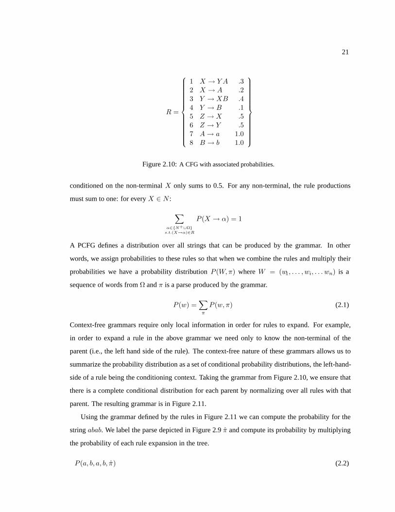
2.10 A CFG with associated probabilities. . . . . . . . . . . . . . . . . . . . . . . . . . . 21

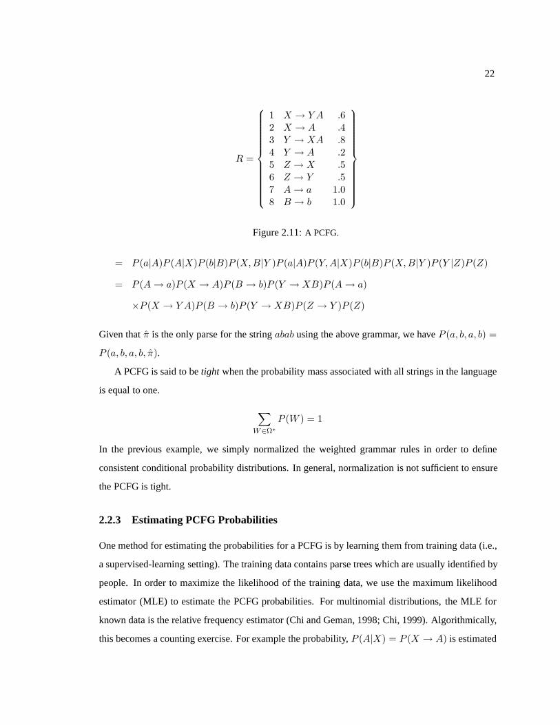
2.11 A PCFG. . . . . . . . . . . . . . . . . . . . . . . . . . . . . . . . . . . . . . . . . 22

2.12 A left-binarized tree. . . . . . . . . . . . . . . . . . . . . . . . . . . . . . . . . . . 24

2.13 Two examples of head-binarized trees. . . . . . . . . . . . . . . . . . . . . . . . . . 25

2.14 A Markov head-binarized tree. . . . . . . . . . . . . . . . . . . . . . . . . . . . . . 26

2.15 A parse of the strings “I saw the man with the telescope” . . . . . . . . . . . . . . . . 28

2.16 Example parse edges for the string “I saw the man with the telescope” . . . . . . . . . . 31

xvi

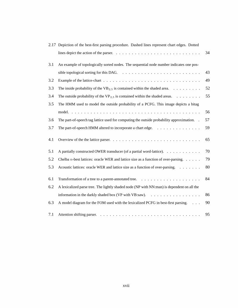
2.17 Depiction of the best-first parsing procedure. Dashed lines represent chart edges. Dotted

lines depict the action of the parser. . . . . . . . . . . . . . . . . . . . . . . . . . . . 34

3.1 An example of topologically sorted nodes. The sequential node number indicates one pos-

sible topological sorting for this DAG. . . . . . . . . . . . . . . . . . . . . . . . . . 43

3.2 Example of the lattice-chart . . . . . . . . . . . . . . . . . . . . . . . . . . . . . . . 49

3.3 The inside probability of the VB2,5 is contained within the shaded area. . . . . . . . . . 52

3.4 The outside probability of the VP2,5 is contained within the shaded areas. . . . . . . . . 55

3.5 The HMM used to model the outside probability of a PCFG. This image depicts a bitag

model. . . . . . . . . . . . . . . . . . . . . . . . . . . . . . . . . . . . . . . . . . 56

3.6 The part-of-speech tag lattice used for computing the outside probability approximation. . 57

3.7 The part-of-speech HMM altered to incorporate a chart edge. . . . . . . . . . . . . . . 59

4.1 Overview of the the lattice parser. . . . . . . . . . . . . . . . . . . . . . . . . . . . . 65

5.1 A partially constructed OWER transducer (of a partial word-lattice). . . . . . . . . . . . 70

5.2 Chelba n-best lattices: oracle WER and lattice size as a function of over-parsing. . . . . . 79

5.3 Acoustic lattices: oracle WER and lattice size as a function of over-parsing. . . . . . . . 80

6.1 Transformation of a tree to a parent-annotated tree. . . . . . . . . . . . . . . . . . . . 84

6.2 A lexicalized parse tree. The lightly shaded node (NP with NN:man) is dependent on all the

information in the darkly shaded box (VP with VB:saw). . . . . . . . . . . . . . . . . 86

6.3 A model diagram for the FOM used with the lexicalized PCFG in best-first parsing. . . . 90

7.1 Attention shifting parser. . . . . . . . . . . . . . . . . . . . . . . . . . . . . . . . . 95

xvii

Chapter 1

Introduction

Over the past decade statistical parsing has matured to the extent that parsing is now incorporated

in other language processing models. Two such tasks that have benefited from parsing are speech

recognition (Charniak, 2001; Roark, 2001a) and machine translation (Charniak and Yamada, 2003),

both using parser-based language models. Initial research on the integration of parsing into a lan-

guage model shows that by considering the structure of language, and specifically the syntactic

structure, we are able to improve the modeling of strings of words (Charniak, 2001; Roark, 2001a;

Chelba and Jelinek, 2000). The focus of this thesis is to extend parsing techniques that have proven

useful for parsing strings in such a way that they are efficient and accurate when used for language

modeling.

We present a novel technique for efficient word-lattice parsing and the means to integrate parser-

based language modeling into word-lattice decoding. Word-lattices are most commonly found in

use by the speech recognition community, but are not specific to speech recognition. Throughout the

thesis, word-lattice parsing is framed in the context of speech recognition although these techniques

extend to any language processing task where the noisy channel model is appropriate (e.g., machine

translation).

The noisy channel model, depicted in Figure 1.1, assumes a noise process that modifies the

source signal, resulting in a noisy copy of the original signal. Applying this to speech recognition,

we assume the speaker has an intended message to communicate which is then passed though the

human speech production system – the true processing channel. The goal of speech recognition

is to recover the original message and is typically accomplished by generating a string of words

1

2

Human SpeechProduction

the man is early...

Input signal Noisy Channel Acoustic Signal

Figure 1.1: Noisy channel model for speech.

(i.e., a transcription). The objective is to automatically transcribe the speech as well as can be done

by a human transcriber. In fact, the performance of speech recognition systems are evaluated by

comparing the output of such systems to human transcriptions. In deriving a generative model for

an automated speech recognition system, we reverse the noisy channel model assumed to produce

the speech signal. Similarly, language translation can be thought of the process of taking a word-

string from one language and 1 passing it through a noisy channel: translation. Again, the goal of

an automated translation system is to recover the original word-string.

The noisy channel model describes a joint distribution P (A,W ) over the set of input speech

acoustics, A, and output word strings W . We express this distribution as P (A,W ) = P (A|W )P (W ),

having applied the definition of conditional probability. From a modeling perspective this splits the

distribution into the noise model (or acoustic model) P (A|W ) and the language model P (W ). The

noise model provides a distribution over possible input word strings given a particular output string.

The language model, as its name suggests, is defined as a distribution of output word strings for

the target language (e.g., English). We model speech using the acoustic model P (A|W ) which is

a conditional distribution over acoustic signals (or features extracted from acoustic signals) given a

particular string of words. Machine translation models based on the noisy channel contain a noise

model that generates sets of translation word-strings given a source-word string from a foreign lan-

guage. If we consider only the word-strings that are given non-zero probability by the noise model,

the noise model can be thought of as a string generator, suggesting a set of hypothetical transcrip-

tions or translations for the input along with a probability for each string. Given this hypothesis set,

we select the string that is most appropriate in the target language, which is accomplished by taking

the string that maximizes the product of the noise model and the language model probabilities (i.e.,

1We will refer to a sequence of words as a word-string or simply a string, when unambiguous, for the remainder ofthe text.

3

maximizing the joint probability of the input and output under the noisy channel model).

Given the joint distribution of source and target word strings and knowing the particular source

(we are either recognizing a specific speech signal or translating a specific foreign word string), we

use the joint distribution to find the most likely target string, W∗.

W ∗ = arg maxW

P (W |A) = arg maxW

P (W,A)P (W )

= arg maxW

P (W,A) (1.1)

Success in language modeling has been dominated by sequential models 2 for the past few

decades; in particular, the n-gram model has become the standard model for production systems

and until recently was the most common found in research systems. Recently, a number of syntactic

language models have proven to be competitive with the n-gram and better than the most popular

n-gram, the trigram (Roark, 2001a; Xu et al., 2002; Charniak, 2001).

One reason that we expect syntactic models to perform well is that they are capable of modeling

long-distance dependencies that simple n-gram models cannot. For example, the model presented

by Chelba and Jelinek (1998; 2002) uses syntactic structure to identify lexical items in the left-

context which are then modeled as an n-gram process. The model presented by Charniak (Charniak,

2001) identifies both syntactic structural and lexical dependencies that aid in language modeling.

While there are n-gram models that attempt to extend the left-context window through the use of

caching and skip models (Goodman, 2001), we believe that linguistically motivated models, such

as these lexical-syntactic models, are more robust. Furthermore, n-gram modeling techniques such

as caching and skip lists can be applied to structure models as well.

Unfortunately, syntactic language modeling techniques have proven to be extremely expensive

in terms of computational effort. Many employ the use of string parsers (Charniak, 2001); in order

to utilize such techniques for language modeling, one must preselect a set of strings from those

hypothesized by the acoustic model and parse each of strings separately, an inherently inefficient

procedure. Other techniques have been designed to adhere to a strict left-to right processing model

(Chelba and Jelinek, 2000; Roark, 2001a), thereby placing constraints on the type of models avail-

able.

In this thesis we explore a global parsing model that utilizes a best-first search strategy. We

present an extension of best-first bottom-up chart parsing of strings to parsing of word-lattices.

2We use the term sequential model to refer to that considers the sequence of words, but no structure over the sequence.

4

0 1yesterday/0

2and/4.004

3in/14.73

4tuesday/0

14tuesday/0 5

to/0.0006

two/8.7697it/51.59

to/0

8outlaw/83.57

9

outline/2.57310

outlined/12.58

outlines/10.71

outline/0

outlined/8.027

outlines/7.14013to/0

in/0

of/115.4

a/71.30

the/115.3 11

strategy/0

strategy/0outline/0

12/0</s>/0

Figure 1.2: A partial word-lattice from the NIST HUB-1 dataset.

Additionally, we describe a coarse-to-fine processing model that utilizes the efficiency of the best-

first search while being able to integrate more sophisticated syntactic language modeling techniques.

1.1 Representing Ambiguity: Word Lattices

A speech utterance contains much more than the words that we associate with it. For example,

knowing the prosody of speech may help in identifying the sequence of words that corresponds to

an utterance. When translating a text, a translation may be influenced by extra-sentential cues that

direct the selection of good translations. However, the most common representation for ambiguous

language (especially in speech) simply identifies a set of hypothetical word-strings annotated with

scores. The scores generally come from the model that predicts these strings, the noise model; in

speech recognition, this is the acoustic model.

Consider a simplified version of the acoustic model used for speech recognition; assume the

model provides an estimate of the probability that an acoustic element (a phone or a phoneme)

occurs during a particular time-frame. These units can be combined to form a variety of strings of

words, typically done through a serious of Hidden Markov Model (HMM) predictions 3 (Jelinek,

1997). Note that a particular string may be predicted multiple times, where the words are predicted

as starting and ending at different points in time. This duplication can be reduce by quantizing the

start and end points of phones, phonemes, etc. (this requires summing the probability for paths that

are quantized). Furthermore, there are many words that are predicted with close to zero probability,

which are pruned, resulting in a set of non-zero probability word-strings as predicted by the acoustic

3The state-of-the-art acoustic modeling techniques tend to make very strong, incorrect independence assumptions(e.g., assuming overlapping phonemes are independent). We note that in many cases, these assumptions are madefor the sake of computational efficiency and modeling simplicity.

5

model.

Enumerating each of the hypothesized strings is simply not tractable; in the worst case, an expo-

nential number 4 of strings pass the acoustic pruning stage; many of these strings contain common

substrings. It is standard to represent these strings in a compact structures called a word-lattice, a

graph that encapsulates a set of word hypotheses along with the scores assigned by the prediction

model; Figure 2.1 is an example of a word lattice. In addition to being a convenient structure for

compactly storing the set of string hypotheses, the word-lattice represents the predictions made by

the acoustic model or the translation model in speech recognition or machine translation respec-

tively. The acoustic prediction probabilities are stored with the words in the arcs of the word-lattice.

Additionally, the lattice may contain probabilities defined by language models. We present the defi-

nition of the word-lattice as well as the standard techniques to compress word-lattices in Section 2.1.

1.2 Language Modeling

In general, the problem of selecting a word-string from a set of hypothesized strings is solved by

deriving a model of all strings in the language. A language model defines a probability distribution

over all of these strings and provides a means to measure the probability of a particular string of

words in the language. Language models can be used to identify the most likely string from a

set of hypothesized strings by evaluating the probability of each word-string. The language model

presented in this thesis not only assigns probability to word-strings but to parses5 of word-strings.

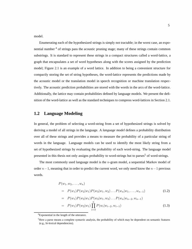
The most commonly used language model is the n-gram model, a sequential Markov model of

order n−1, meaning that in order to predict the current word, we only need know the n−1 previous

words.

P (w1, w2, . . . , wn)

= P (w1)P (w2|w1)P (w3|w1, w2) . . . P (wn|w1, . . . , wn−1) (1.2)

= P (w1)P (w2|w1)P (w3|w1, w2) . . . P (wn|wn−2, wn−1)

= P (w1)P (w2|w1)n∏

i=3

P (wi|wi−2, wi−1) (1.3)

4Exponential in the length of the utterance.5Here a parse means a complete syntactic analysis, the probability of which may be dependent on semantic features(e.g., bi-lexical dependencies).

6

Equation 1.2 6 follows from the chain rule and Equation 1.3 comes from applying the Markov

assumption for a Markov process of order 2.

State-of-the-art commercial language modeling techniques for speech recognition use trigrams,

while state-of-the-art research in n-gram modeling use up to 20-grams with a melange of techniques

used to make the models tractable (Goodman, 2001).

1.3 Parsing and Language Modeling

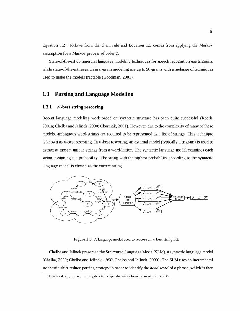
1.3.1 N-best string rescoring

Recent language modeling work based on syntactic structure has been quite successful (Roark,

2001a; Chelba and Jelinek, 2000; Charniak, 2001). However, due to the complexity of many of these

models, ambiguous word-strings are required to be represented as a list of strings. This technique

is known as n-best rescoring. In n-best rescoring, an external model (typically a trigram) is used to

extract at most n unique strings from a word-lattice. The syntactic language model examines each

string, assigning it a probability. The string with the highest probability according to the syntactic

language model is chosen as the correct string.

w1, ..., wi, ..., wn1

...

LanguageModel

w1, ..., wi, ..., wn2

w1, ..., wi, ..., wn3

w1, ..., wi, ..., wn4

w1, ..., wi, ..., wnm

o1, ..., oi, ..., on

8

2

3

5

1 6

4

7 10

9

the/0

man/0

is/0

duh/1.385

man/0 is/0surely/0

early/0

mans/1.385

man's/1.385

surly/0

surly/0.692

early/0

early/0 n-best list

extractor

Figure 1.3: A language model used to rescore an n-best string list.

Chelba and Jelinek presented the Structured Language Model(SLM), a syntactic language model

(Chelba, 2000; Chelba and Jelinek, 1998; Chelba and Jelinek, 2000). The SLM uses an incremental

stochastic shift-reduce parsing strategy in order to identify the head-word of a phrase, which is then

6In general, w1, . . . , wi, . . . , wn denote the specific words from the word sequence W .

7

incorporated into a head-word n-gram model. The SLM executes a beam-search to build partial

parses of the string which are used to identify head-words. Since the head-word model requires

only that the most recent n − 1 head-words be known, parses need not be extended beyond a point

at which this information is available. The SLM can process word-lattices directly, but does not

perform better than when restricted to n-best lists.

The SLM does not attempt to provide a complete syntactic analysis, yet provides a means to

identify non-local lexical dependencies 7. Non-local dependencies are critical in identifying models

that are more robust than the typical n-gram model. The idea of using syntactic structure to identify

non-local lexical dependencies is common among the syntactic language models presented here.

Roark proposes a syntactic language model that operates in a left-to-right manner (Roark,

2001b; Roark, 2001a) using a top-down, left-corner parser. As with the SLM, a beam-search is

used to extend the parses. The parser achieves accuracy approaching some of the best probabilistic

parsers, although beam size does limit the parser’s coverage (as is discussed in detail in (Roark,

2001b)). More recently, Roark proposed a model that is capable of parsing n-gram word-lattices

which contained 1000-best strings extracted from acoustic lattices (Roark, 2002). Roark points out

that this technique is also capable of rescoring the word-arcs of the word-lattices, something not pos-

sible using rescoring techniques. The language model defined by this Roark parser is competitive

with other syntactic language modeling techniques.

Charniak introduced a version of his probabilistic bottom-up/top-down lexicalized parser that

assigns language model probabilities 8 (Charniak, 2001). This parser works in two stages: first,

an impoverished grammar (a PCFG) is used to provide a set of candidate parses; and second, a

lexically-based syntactic language model selects the best parse and assigns it a probability under the

model. As our parser works in a similar manner, we provide details later in the thesis. Currently, the

Charniak parser-based language model performs better than any other language model (including

the previously mentioned syntactic language models) on the NIST ’93 HUB-1 dataset. This thesis

describes work that extends the techniques used by the Charniak parser to the parsing of word-

lattices.7The SLM is extended to a full parsing model in (Chelba, 2000).8The probabilities are assigned globally by the parser, but are able to be extracted on a word-per-word bases in orderto compute measures such as perplexity, etc.

8

1.3.2 Lattice Parsing

Unlike the techniques described in the previous section, word-lattice parsing does not require n-

best lists to be preselected from the acoustic lattices. By allowing our syntactic language modeling

technique to analyze any of the word-string from the original acoustic lattice, the upper-bound on

our performance is only limited by the quality of the acoustic model. N -best techniques can do no

better than selecting the best string from a preselected list. As we show in our analysis, the string

or the n-best strings closest to the correct string (the reference transcription) is often not as close

as the best string contained in the acoustic lattices (i.e., the best string has been pruned during the

n-best selection process).

We are not the first to attempt to design a lattice-based chart parsing algorithm. Hans Webber

proposed a similar bottom-up chart parsing technique based on a pseudo-probabilistic unification-

based grammar (Weber, 1994). Chappelier, et. al. describe a word-lattice parsing technique based

on a standard CKY parser (Chappelier et al., 1999). In work published concurrently with the writ-

ing of this thesis, Chris Collins has developed a word-lattice capable version of the Collins parser

(Collins et al., 2004; Collins, 2003). The work presented in this thesis includes published results

(Hall and Johnson, 2003; Hall and Johnson, 2004) which, to the best of our knowledge are the first

results of using a word-lattice parser for language modeling.

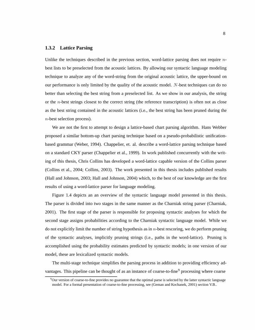
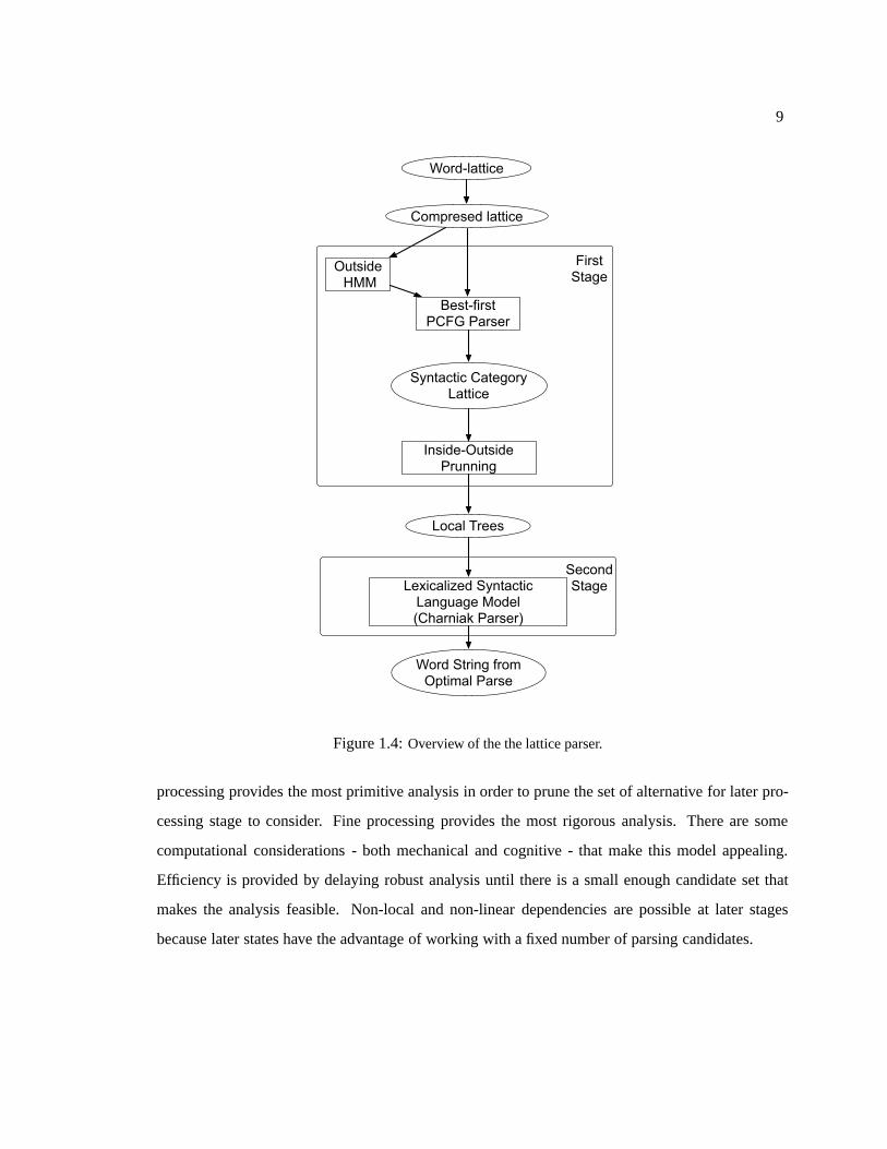
Figure 1.4 depicts an an overview of the syntactic language model presented in this thesis.

The parser is divided into two stages in the same manner as the Charniak string parser (Charniak,

2001). The first stage of the parser is responsible for proposing syntactic analyses for which the

second stage assigns probabilities according to the Charniak syntactic language model. While we

do not explicitly limit the number of string hypothesis as in n-best rescoring, we do perform pruning

of the syntactic analyses, implicitly pruning strings (i.e., paths in the word-lattice). Pruning is

accomplished using the probability estimates predicted by syntactic models; in one version of our

model, these are lexicalized syntactic models.

The multi-stage technique simplifies the parsing process in addition to providing efficiency ad-

vantages. This pipeline can be thought of as an instance of coarse-to-fine9 processing where coarse

9Our version of coarse-to-fine provides no guarantee that the optimal parse is selected by the latter syntactic languagemodel. For a formal presentation of coarse-to-fine processing, see (Geman and Kochanek, 2001) section V.B..

9

Compresed lattice

Outside HMM

Best-firstPCFG Parser

Syntactic CategoryLattice

Inside-OutsidePrunning

Local Trees

Lexicalized SyntacticLanguage Model(Charniak Parser)

Word String fromOptimal Parse

Word-lattice

FirstStage

SecondStage

Figure 1.4: Overview of the the lattice parser.

processing provides the most primitive analysis in order to prune the set of alternative for later pro-

cessing stage to consider. Fine processing provides the most rigorous analysis. There are some

computational considerations - both mechanical and cognitive - that make this model appealing.

Efficiency is provided by delaying robust analysis until there is a small enough candidate set that

makes the analysis feasible. Non-local and non-linear dependencies are possible at later stages

because later states have the advantage of working with a fixed number of parsing candidates.

10

1.3.3 Structure of this Thesis

In the next chapter, we present a tutorial covering the background concepts and techniques re-

quired by our lattice parser. The background material is intended to be a review of the Probabilistic

Context-Free Grammars (PCFG), the compression of Weighted Finite State Automata, and the tech-

niques used for best-first probabilistic parsing. In Chapter 3 we introduce the general coarse-to-fine

parsing model that we have adopted. Following, we focus on best-first word-lattices parsing using

a PCFG and the integration of this into a syntactic language model. Next, we present a set of ex-

periments that explore the performance of both stages of our complete syntactic language modeling

system. In Chapter 6 we explore alternate grammars to be used with the best-first parser. In Chap-

ter 7 we address the question of whether our model may do better if we were to force the parser

to shift attention to parts of the word lattice with few or no analyses. We report the results of ex-

periments performed with each model and provide some some analysis of these results. Finally we

provide a summary and a discuss the potential for future work.

Chapter 2

Background

2.1 Word-Lattices

0

8

2

3

5

16

4

7 10

9<s>/0

the/0

man/0

is/0

duh/1.385

man/0 is/0

surely/0

early/0man's/1.385

mans/1.385

surly/0

early/0

surly/0.692

early/0

11/0.916</s>/0

Figure 2.1: A sample word-lattice presented as a finite state machine.

The word-lattice provides a compact representation for a set of word-strings along with scores

associated with the strings. Similarly, a finite state machine (FSM) defines a set of strings, and a

weighted finite state machine (WFSM) is a mapping of a set of strings to scores. In this section

we describe how we transform a word-lattices into a Weighted Finite State Machine (WFSM) and

how we benefit from this conversion. Weighted FSMs are a variation of the FSM and provide

both a formalism and a set of standard algorithms that allow us to work with the word-lattice more

efficiently.

11

12

The most important computational tools we use are that of WFSM determinization and mini-

mization. A determinized FSM takes a potential nondeterministic FSM and creates a deterministic

FSM by ensuring that there is at most one path for any string prefix. Through WFSM minimization

the suffixes of the graph are also compressed into single paths. Reducing the size of the word-lattice

through these operations increases the amount of structure sharing between word-strings. As we

describe later in the thesis, this directly affects the amount of structure sharing available when pars-

ing which dramatically reduces the computational effort needed to explore syntactic analyses over

the entire word-lattice.

2.1.1 Raw Word-lattice Format

Prior to performing any processing over the word-lattice, we transform the lattice from raw format

into a WFSM. We present a process for transforming a word-lattice into a WFSM using the raw

word-lattice Structure Lattice Format (SLF) provided by the HTK toolkit (a set of general tools for

building Hidden Markov Models for speech recognition (Young et al., 2002)). It should be clear

that any raw word-lattice format can be transformed into a WFSM.

The HTK SLF word-lattice is a collection of nodes and an adjacency list (the arcs), a unique

start symbol and a unique end symbol. Word labels are associated with either nodes or arcs, but we

consider the case where the arcs are labeled. In general, the start-of-utterance labels are unnecessary

so long as we can identify a start node (i.e., we assume that the acoustic alignment procedure

provides us with word-lattices beginning at the same time). As we concatenate common suffixes, it

helps to know that every path in the lattice terminates at the same node. To do this, we utilize the

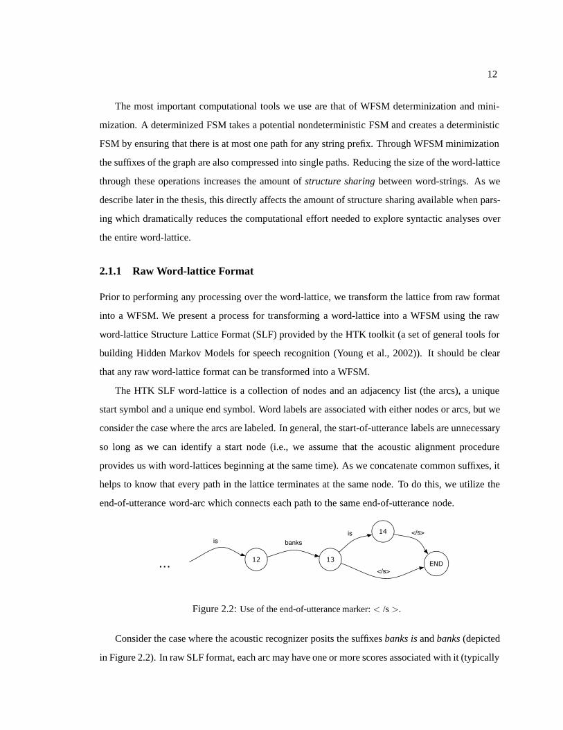
end-of-utterance word-arc which connects each path to the same end-of-utterance node.

END12 13

banks

14is

</s>

is

...

</s>

Figure 2.2: Use of the end-of-utterance marker: < /s >.

Consider the case where the acoustic recognizer posits the suffixes banks is and banks (depicted

in Figure 2.2). In raw SLF format, each arc may have one or more scores associated with it (typically

13

log-probabilities) corresponding to the acoustic model, n-gram model, and other arbitrary language

models.

CONVERTLATTICE(N ,A, s∗)1 remove start-of-utterance node s∗

2 for j ∈ N such that s∗ → j ∈ A3 do j ← 0 // new start node4 for ia,b ∈ A // an arc from node a to node b5 do label(ia,b) ← label(b)6 for node k ∈ L7 do label(k) ← null

Table 2.1: A function to convert a node-labeled FSM to an arc-labeled FSM.

For the remainder of the thesis, we only consider arc-labeled graphs (word-lattices and FSMs).

When the input word-lattice is not originally arc-labeled (i.e., it is node labeled), we can transform

it into a node labeled graph. This is the similar transformation to that of converting a Moore FSM

(output labeled depend on the current state) into a Mealy FSM (output labels depend on the previous

state and the current state). The transformation maps a node-labeled graph G, composed of nodes

N , arcs A, and start state s∗, into an arc-labeled graph. This transformation is presented in Table 2.1.

The word-lattice is clearly a directed acyclic graph (DAG), a characteristic necessary for effi-

cient FSM manipulations. This fact is obvious with speech word-lattices as they encode a time-

based sequential process (the acoustic signal), preventing cyclic structure in the word-lattice.

2.1.2 Finite State Machines

FSM word-lattices are not new; finite state machine representations of word-lattices are quite com-

mon in the speech recognition research community. Due to the global structure of the parsing mod-

els we use, we are able to take advantage of FSM manipulations that may be difficult or impossible

with alternative parsing techniques. This is due to the fact that the weighted FSM transformations

shift probability mass along lattice paths in order to best compress the lattice; the probability asso-

ciated with any particular word-lattice path (a string) remains the same. An algorithm that considers

only a subset of the lattice in order to direct a search may be misguided by the transformed word-

lattice. Algorithms that use the probability associated with the entire word-lattice or any complete

path in the word-lattice, such as our word-lattice parser, will not be effected by the transformations.

14

A weighted FSM generates a set of sequences and assigns a score (or weight) to each sequence.

Generally, the score assigned to the sequence is simply the sum of arc-scores along the path de-

scribing the sequence. We record the log-probability of the word being generated given the model

for on each word-arc. The score associated with a sequence accepted/generated by the FSM is the

sum of the word-arc scores. In other words, we store the acoustic log-probability, ln (p (ai|wi)) for

each arc i 1, where the string is W = (w1, . . . , wi, . . . , wn). Assuming the model distributions are

conditionally independent (for each word), the probability of the string is defined as:

P (A|W ) =∏

wi∈W

p(ai|wi) = exp

∑

wi∈W

ln (p (ai|wi))

FSM Transformations

man

1

2 3 4 5

the

is early

</s>

7 8 9is surly

</s>

11 12early </s>

mans13 14 15

the

surly</s>

man

mans

Figure 2.3: A simple FSM.

Consider a standard FSM acceptor (without scores) as presented in Figure 2.3. Clearly, there are

four unique sequences that this FSM accepts (generates). There is also quite a bit of duplication in

this FSM. We present two transformations that preserve the functionality of the FSM while resulting

in a more compact representation: determinization and minimization.

The FSM in Figure 2.3 is not deterministic. There are multiple paths leading from node 1 that

accepts the word the. Similarly, there are multiple transitions from node 2 and node 13 that accept

identical words. Determinization is the process of collapsing nodes to create a deterministic FSM.

In a deterministic FSM, there is only one path that accepts each unique prefix.

The lattice in Figure 2.4 has been determinized. Note that there is still some duplication that

can be removed. There are multiple transitions with identical labels leading to the termination node.

We reduce this duplication through a process called minimization.1The base of the logarithm is irrelevant so long as we use the same base when converting back to probability space.

15

man

1 2

3 4 5

the

is early

</s>

9

surly

</s>

11 12early </s>

15

surly </s>

mans

Figure 2.4: A determinized FSM.

man

1 2

3

4

5theis

early </s>

9surly </s>

mans

Figure 2.5: A determinized and minimized FSM.

The lattice in Figure 2.5 has been determinized and minimized. In general, we can take any sub-

lattice of a lattice and perform the minimization. It is important to note that determinization and

minimization do not allow new strings to be accepted by the FSM; these transformations strictly

preserve the set of strings defined by the FSM.

Weighted FSM Transformations

The word-lattice FSMs that we use are weighted FSMs (WFSM). We want to compact the WFSM

in the same manner as the FSM above, but we also want to preserve the scores associated with

sequences. Since we only care about the scores assigned to the unique sequences accepted by the

FSM we can perform similar determinization and minimization transformations.

Mehryar Mohri and the FSM group at AT&T have developed efficient minimization and deter-

minization algorithms for WFSMs (Mohri et al., 1998; Mohri et al., 2000; Mohri et al., 2002). They

have also developed a number of other useful tools for manipulating weighted WFSMs (e.g. n-best

path generation).

Weighted FSMs introduce additional complexity to the determinization and minimization pro-

cesses; the resulting FSM not only accepts the same set of sequences as the original FSM but it

16

also preserves the cumulative weight for any sequence accepted by the FSM. The following ex-

ample provides the same step-by-step presentation of FSM determinization and minimization for

weighted FSMs.

0 1<s>/0

2the/0.104

6the/0.104

9the/0.104

12

the/0.104

15

the/0.104

19

duh/0.230

3man/0.693

7man’s/1.608

10mans/1.204

13mans/1.204

16man/0.693

20man/0.693

4is/0

5early/0.509 23/0</s>/0

8early/0.509

24/0</s>/0

11early/0.509 25/0</s>/0

14surly/1.204

26/0</s>/0

17is/0

18surly/1.204

27/0</s>/0

21

is/0

22surely/1.608

28/0</s>/0

Figure 2.6: A weighted FSM.

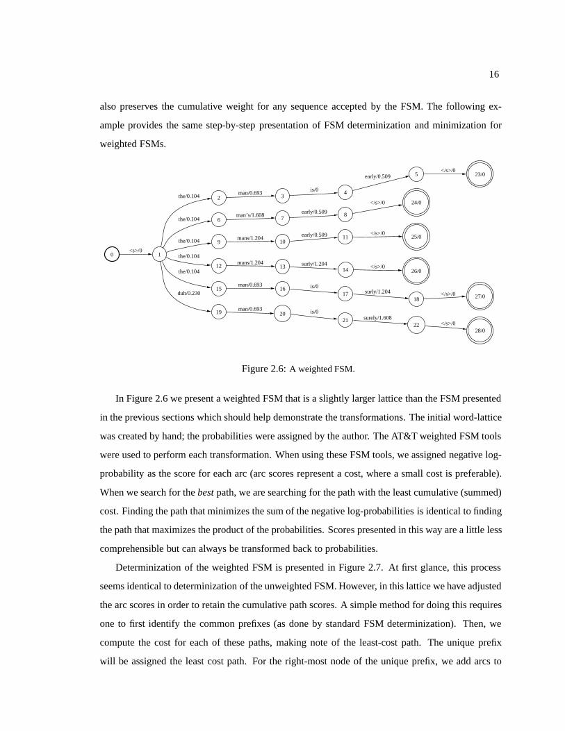
In Figure 2.6 we present a weighted FSM that is a slightly larger lattice than the FSM presented

in the previous sections which should help demonstrate the transformations. The initial word-lattice

was created by hand; the probabilities were assigned by the author. The AT&T weighted FSM tools

were used to perform each transformation. When using these FSM tools, we assigned negative log-

probability as the score for each arc (arc scores represent a cost, where a small cost is preferable).

When we search for the best path, we are searching for the path with the least cumulative (summed)

cost. Finding the path that minimizes the sum of the negative log-probabilities is identical to finding

the path that maximizes the product of the probabilities. Scores presented in this way are a little less

comprehensible but can always be transformed back to probabilities.

Determinization of the weighted FSM is presented in Figure 2.7. At first glance, this process

seems identical to determinization of the unweighted FSM. However, in this lattice we have adjusted

the arc scores in order to retain the cumulative path scores. A simple method for doing this requires

one to first identify the common prefixes (as done by standard FSM determinization). Then, we

compute the cost for each of these paths, making note of the least-cost path. The unique prefix

will be assigned the least cost path. For the right-most node of the unique prefix, we add arcs to

17

0 1<s>/0

2the/0.104

3

duh/0.230

4man/0.693

5mans/1.204

6

man’s/1.608

7man/0.693

8is/0

9early/0.509

10surly/1.204

11

early/0.509

12is/0

13early/0.509

14surly/1.204

15/0</s>/0

16/0</s>/0

17/0</s>/0

18surely/1.608

19/0</s>/0

20/0</s>/0

21/0</s>/0

Figure 2.7: A determinized weighted FSM.

the tail of each of the paths whose prefixes were collapsed. The label on this arc is retained from

the original path, but weight on this arc will be adjusted. The weight is adjusted by the difference

between the least cost prefix and the cost of the prefix for the original path (i.e., the path that used

to extend to the next node past the common prefix). In this way, the cost of the path for each string

is identical to the original cost, but common prefixes have been concatenated.

0 1<s>/0

2the/0

3

duh/1.223

4man/0

5mans/0.510

6

man’s/0.916

9man/0

is/0

7

early/0

surly/0.694

early/0

10is/0

8/1.307</s>/0

surely/0

Figure 2.8: A determinized and minimized weighted FSM.

Figure 2.8 is the determinized and minimized version of Figure 2.6. Minimization is a more

complicated for weighted FSMs. First, we have the same constraints that we had with the regular

FSM: sub-lattices can be combined if they contain the identical set of arcs. Additionally, in a

weighted FSM, sub-lattices can be combined if each arc with the same label has the same score. A

process called weight pushing (Mohri and Riley, 2001) allows for the redistribution of arc weights

while preserving total path costs. Weight pushing is performed prior to minimization in order to

18

transform identically labeled sub-lattices into sub-lattices that also have identical weights. Regular

FSM minimization is performed on the weighted FSM by combining the labels and weights into

new labels.

Certainly, some intricacies have been omitted in this brief presentation. For an exhaustive

presentation of weighted FSMs and the details of the determinization, minimization, and weight-

pushing algorithm please see Mohri et al. (1998; Mohri et al. (2000; Mohri et al. (2002).

Weighted FSMs and Parsing

Consider a word-lattice parsing algorithm that processes the lattice sequentially from left to right

performing a beam search such as the Roark (Roark, 2001a) and Chelba (Chelba and Jelinek, 2000)

techniques. Scores on the arcs are critical in determining which paths are included in the beam

search. The weight-pushing algorithm we described above is capable of moving sub-lattice path

weights in order to facilitate minimization, etc. Doing so may inadvertently distort the score of a

path in the word-lattice, delaying the realization of the acoustic score until a later time. This has

the potential to guide a sequential greedy search technique towards paths with lower likelihood (as

realized when the entire path has been processed).

One solution is to make sure the weight pushing algorithm always pushes weight towards the

start node. Additionally, the look-ahead (as used by a sequential parser) must account for weight

movement.

In the parser presented in this thesis, the weight of entire lattice paths are considered rather than

the arc weights in isolation. In other words, the parser considers the entire lattice and performs

a search over the lattice in a global manner, thereby rendering the parsing algorithm resilient to

weight movement in the word-lattice. Therefore, the WFSM manipulations as presented in this

section have no effect on the search performed by the parser. Instead, these manipulations provide

a representation of the word-strings that allows for increased structure sharing during parsing, thus

resulting in a more efficient parsing algorithm. We describe structure sharing more in Chapter 3.

19

2.2 Probabilistic Context Free Grammars

A Probabilistic Context Free Grammar (PCFG) is a probabilistic model over a set of parse trees (this

set may be countably infinite). A parse tree is a hierarchical structure that represents a particular

grammar derivation. In this chapter we provide a brief review of PCFGs and present variations of

the PCFG that are useful for our parsing algorithm. A complete presentation of PCFGs as used for

Natural Language Processing (NLP) can be found in Manning and Shutze (1999), Charniak (1993;

1997), Geman and Johnson (Geman and Johnson, 2003), and Collins (1999).

2.2.1 Context Free Grammar

Context Free Grammars (CFGs) are relatively common in the fields of linguistics and computer

science. In the former, CFGs provide the simplest model of language processing. CFGs are well

known to be inadequate in describing the complex interdependencies of human language, which are

anything but context-free. Computer scientists use CFGs to describe the vast collection of artificial

languages used by computers.

A CFG is a quadruple, G = Ω, N, s, R where Ω and N are disjoint sets. Ω is the set of

terminal symbols (e.g., the words in the vocabulary of the language), N is a set of non-terminal

symbols, and the symbol s ∈ N is a special start symbol from the set of non-terminals. The set

R ⊆ (N → N+) ∪ (N → Ω) is a set of productions which describe non-terminal rewrite rules.

We define T ⊂ N to be the set of non-terminals the expand to terminal rules (i.e., t ∈ T : (t → ω)

where ω ∈ Ω). These are called the preterminals 2. For example, assume a simplified grammar that

produces strings of a’s and b’s.

Example sentences produced by the grammar in Table 2.2 are abab and bababa. In Figure 2.9

we show a parse tree for the sentence abab. The parse tree presents the hierarchical description of

rule application. In this case, rule 6 generated Y to which rule 1 was applied, generating Y A. Rule

3 is then applied to the Y and so on. Depending on the grammar, there are likely to be many parses

for each unique sentence.

2A CFG that describes the syntactic structure of a natural language typically maps the preterminals to part-of-speechtags.

20

• Ω = a, b

• N = A,B,X, Y,Z

• T ⊂ N = A,B

• s = Z

• R =

1 X → Y A2 X → A3 Y → XB4 Y → B5 Z → X6 Z → Y7 A → a8 B → b

Table 2.2: An example CFG.

Y

X

Y

X

A

B

A

B

Z

a

b

b

a

Figure 2.9: A parse of the strings abab

2.2.2 Probabilities and Context Free Grammars

Probabilistic Context Free Grammars (PCFG) are a type of weighted CFGs: a CFG in which a

weight is assigned to each rule. In order to compute the weight of a particular parse (associated

with a parse tree), we multiply the weights of each rule application in the parse. Much as with the

the weighted FSM, we can use probabilities or log-probabilities: however, if we use the later, we

sum the weights rather than multiplying. In Figure 2.10 we have assigned random probabilities to

each rule. This is not a PCFG, because we have deficient conditional probability distributions (i.e.,

the sum of the probability over the dependent events is not equal to 1). For example, the distribution

21

R =

1 X → Y A .32 X → A .23 Y → XB .44 Y → B .15 Z → X .56 Z → Y .57 A → a 1.08 B → b 1.0

Figure 2.10: A CFG with associated probabilities.

conditioned on the non-terminal X only sums to 0.5. For any non-terminal, the rule productions

must sum to one: for every X ∈ N :

∑α∈N+∪Ω

s.t.(X→α)∈R

P (X → α) = 1

A PCFG defines a distribution over all strings that can be produced by the grammar. In other

words, we assign probabilities to these rules so that when we combine the rules and multiply their

probabilities we have a probability distribution P (W,π) where W = (w1, . . . , wi, . . . wn) is a

sequence of words from Ω and π is a parse produced by the grammar.

P (w) =∑π

P (w, π) (2.1)

Context-free grammars require only local information in order for rules to expand. For example,

in order to expand a rule in the above grammar we need only to know the non-terminal of the

parent (i.e., the left hand side of the rule). The context-free nature of these grammars allows us to

summarize the probability distribution as a set of conditional probability distributions, the left-hand-

side of a rule being the conditioning context. Taking the grammar from Figure 2.10, we ensure that

there is a complete conditional distribution for each parent by normalizing over all rules with that

parent. The resulting grammar is in Figure 2.11.

Using the grammar defined by the rules in Figure 2.11 we can compute the probability for the

string abab. We label the parse depicted in Figure 2.9 π and compute its probability by multiplying

the probability of each rule expansion in the tree.

P (a, b, a, b, π) (2.2)

22

R =

1 X → Y A .62 X → A .43 Y → XA .84 Y → A .25 Z → X .56 Z → Y .57 A → a 1.08 B → b 1.0

Figure 2.11: A PCFG.

= P (a|A)P (A|X)P (b|B)P (X,B|Y )P (a|A)P (Y,A|X)P (b|B)P (X,B|Y )P (Y |Z)P (Z)

= P (A → a)P (X → A)P (B → b)P (Y → XB)P (A → a)

×P (X → Y A)P (B → b)P (Y → XB)P (Z → Y )P (Z)

Given that π is the only parse for the string abab using the above grammar, we have P (a, b, a, b) =

P (a, b, a, b, π).

A PCFG is said to be tight when the probability mass associated with all strings in the language

is equal to one.

∑W∈Ω∗

P (W ) = 1

In the previous example, we simply normalized the weighted grammar rules in order to define

consistent conditional probability distributions. In general, normalization is not sufficient to ensure

the PCFG is tight.

2.2.3 Estimating PCFG Probabilities

One method for estimating the probabilities for a PCFG is by learning them from training data (i.e.,

a supervised-learning setting). The training data contains parse trees which are usually identified by

people. In order to maximize the likelihood of the training data, we use the maximum likelihood

estimator (MLE) to estimate the PCFG probabilities. For multinomial distributions, the MLE for

known data is the relative frequency estimator (Chi and Geman, 1998; Chi, 1999). Algorithmically,

this becomes a counting exercise. For example the probability, P (A|X) = P (X → A) is estimated

23

by:

P (X → A) =C(X → A)

C(X)(2.3)

where C(A,X) count the the number of times we have seen the rule (X → A) in our training data

and C(X) is the number of times we have seen a rule with X on the left-hand-side. When trained by

the relative frequency estimator, the PCFG distribution is tight, meaning that the probability mass

assigned to the training examples is equal to 1.

With more complex grammars, we can’t expect to observe all configurations within the training

data. This is even true of the preterminal distribution in a vanilla PCFG. The preterminal rule

P (NN → dog) must be estimated from observations of the word dog being used as a NN . We

expect to run our parser on novel text so we cannot assume that we will have observed all possible

lexical items. In order to reserve some probability mass for unknown items we perform smoothing,

the process of guessing the likelihood of unknown events given a context. In this theses we have

explored simple smoothing techniques such as Laplacian smoothing (and Jeffrey–Perks smoothing)

as well as more reliable techniques such as Jelinek–Mercer EM smoothing. Smoothing is a bit of

an art so we explored those techniques that have been reported to work well and were easy enough

to implement. For a excellent analysis of smoothing techniques as applied to n-gram modeling

for speech recognition, see (Goodman, 2001). We describe the specific details of the smoothing

techniques we use in Chapters 5 and 6.

2.2.4 Binarization

A grammar is said to be binary if each of its rules has at most two constituents on the right-hand

side (the grammars presented in the previous section are binary grammars). A binary grammar is a

relaxation of the Chomsky Normal Form (CNF) grammar which constrains the rules of the grammar

to be either binary non-terminal branches (a non-terminal expanding to two non-terminals) or a

preterminal rule. Binary grammars have rules of the form (where X,Y,Z ∈ Z and w ∈ Ω):

X → Y Z

X → Y

X → w

24

The CKY parsing algorithm for a binarized grammar maintains the same efficiency guarantees as

with a CNF grammar. By relaxing the CNF constraints, the grammar is capable of representing

unary non-terminal transitions that may capture some interesting syntactic phenomena.

BINARIZE(G = Ω, N, s,R)1 for r ∈ R : (x → y1 · · · yn) where n ≥ 32 do z ← y2 · · · Yn // create a new binary category3 N ← N ∪ z // add new category to grammar’s non-terminal set4 replace r in R with (x → y1z)5 R ← R ∪ (z → y2 · · · yn)// add new binarized rule to grammar

Table 2.3: A tree binarization function.

A grammar that has more than two constituents on the right-hand side can be transformed into

a binary grammar. Trees are transformed using the function in Table 2.3, where the is a con-

catenation function. The above procedure describes what is known as bottom-up right-binarization,

a procedure which creates grammars that are right branching wherever there were more than two

constituents in the original grammar. The corresponding left-binarization procedure should be self-

evident. Figure 2.12 depicts the effect of left-binarization on a partial parse tree.

the grey car

DT JJ NN

NP

the grey

carDT JJ

NN

NP

DT JJ

Figure 2.12: A left-binarized tree.

The PCFG for a binarized grammar is estimated in the same way as with the original grammar,

using the relative frequency estimator. Binarized PCFGs define the same probability model as the

original PCFG; for any string in the language both PCFGs assign it the same probability. Efficient

(O(n3)) PCFG parsing algorithms either perform on-the-fly binarization (as is accomplished by

using Early style dotted rules) or explicitly binarize the grammar prior to parsing. Forcing right-

branching, left-branching, or some mixture of the two allows us to capture more or less contextual

information. The total probability associated with the parses of a string will be the same regardless

of the binarization scheme. However, if we use the probability associated with partial analyses to

direct a search for a subset of all parses, then some binarization scheme may be more favorable than

25

others.

The training procedure over binarized trees is identical as to that with the complete trees. We

use the maximum likelihood (relative frequency) estimator to collect statistics for each local tree

configuration. We are then able to use the learned distribution to assign probability to a new tree

simply by computing the local probabilities and taking the product of all local probabilities (this is

true due to fact that under a CFG, the local trees are generated independently of each other).

the grey car

DT JJ NN

NP

Lincoln

PRN

town

NN

the grey car

DT JJ NN

NP

Lincoln

PRN

town

NN

NN (NN)

PRN NN (NN)

JJ PRN NN (NN)

VP

had already sold the car

VBN DT NNRBVB

ADVP NP

VP

VP

had already sold the car

VBN DT NNRBVB

ADVP NP

VP

ADVP (VP)

Figure 2.13: Two examples of head-binarized trees.

Finally, one can choose a linguistically motivated binarization scheme such as head-binarization.

The head-word of a phrase is defined as the salient word in the phrase. Head-words are important in

the determining the semantic content of a sentence and were originally identified early on in work on

formal models of human syntax (Chomsky, 1970; Harris, 1951). In Chapter 6 we describe an algo-

rithm that deterministically identifies head-words from syntactic parser trees. In head-binarization,

the head-word is used to determine how binarization is performed. We may choose to binarize

starting from the head and moving to the left of the head, or moving to the right of the head. In

Figure 2.13 we show two trees that have been head-binarized. In this example, we encoded the po-

sition of the head-word in the binarized category by placing it within parentheses. This information

provides additional context about the parent; it not only determines what the children categories

are (which the previously described binary categories also provided), but it also indicates which of

26

these children is the head child. A PCFG parser with head-child annotations typically does not per-

form any better than a standard PCFG parser, but head-binarization is necessary when incorporating

lexical dependencies into the model.

2.2.5 Markovization

the grey car

DT JJ NN

NP

Lincoln

PRN

town

NN

the grey car

DT JJ NN

NP

Lincoln

PRN

town

NN

NN (NN)

PRN - (NN)

JJ - (NN)

Figure 2.14: A Markov head-binarized tree.

Markovization is a variation of grammar binarization and the procedure is similar to the bina-

rization procedure. In step 4 of the binarization procedure described above, we may choose to label

the rule with something other then the concatenation of the constituent labels. Depending on the

parsing model (bottom-up, top-down, etc.) we may want to record different information about the

binarization step. When Markovizing the grammar, we choose to forget some of this information.

In fact we choose to systematically remember a limited contextual window, making the Markov

assumption that the distribution will not be much different than the distribution conditioned on the

complete context (a false assumption, but one that provides some practical benefit when parsing).

Figure 2.14 depicts a Markov head-binarized transformation. Note that we use the ‘−’ to indicated

that there has been something removed from the context. This provides a limited amount of con-

text that allows us to differentiate between those deterministic binarized rules (those whose label

explicitly indicates the children) and those which have been created by Markovization.

Once we have transformed the binarization procedure to record the abbreviated information in

our binarized categories, we can simply train our PCFG on the new trees. Markovization has the

effect of collapsing categories and rules in the grammar. For example, assume we Markovize by

removing all internal constituent labels for any binarized category. The following categories, when

27

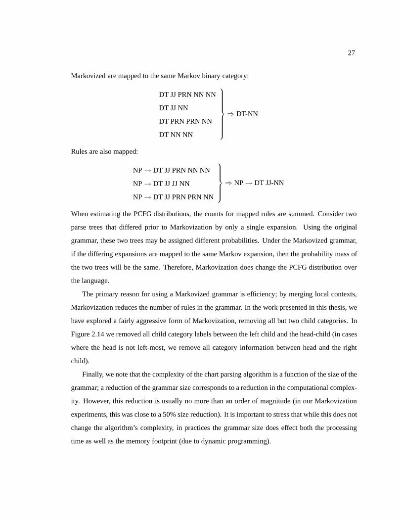
Markovized are mapped to the same Markov binary category:

DT JJ PRN NN NN

DT JJ NN

DT PRN PRN NN

DT NN NN

⇒ DT-NN

Rules are also mapped:

NP → DT JJ PRN NN NN

NP → DT JJ JJ NN

NP → DT JJ PRN PRN NN

⇒ NP → DT JJ-NN

When estimating the PCFG distributions, the counts for mapped rules are summed. Consider two

parse trees that differed prior to Markovization by only a single expansion. Using the original

grammar, these two trees may be assigned different probabilities. Under the Markovized grammar,

if the differing expansions are mapped to the same Markov expansion, then the probability mass of

the two trees will be the same. Therefore, Markovization does change the PCFG distribution over

the language.

The primary reason for using a Markovized grammar is efficiency; by merging local contexts,

Markovization reduces the number of rules in the grammar. In the work presented in this thesis, we

have explored a fairly aggressive form of Markovization, removing all but two child categories. In

Figure 2.14 we removed all child category labels between the left child and the head-child (in cases

where the head is not left-most, we remove all category information between head and the right

child).

Finally, we note that the complexity of the chart parsing algorithm is a function of the size of the

grammar; a reduction of the grammar size corresponds to a reduction in the computational complex-

ity. However, this reduction is usually no more than an order of magnitude (in our Markovization

experiments, this was close to a 50% size reduction). It is important to stress that while this does not

change the algorithm’s complexity, in practices the grammar size does effect both the processing

time as well as the memory footprint (due to dynamic programming).

28

2.3 Efficient Probabilistic Chart Parsing

Parsing is the process of assigning linguistic structure to the sentences of a language. Over the past

decade or so, statistical parsing techniques have proven to be very effective. The statistical parsing

algorithms are based on generative models of the language as defined by a grammar such as the

PCFG described in the previous section.

A parse represents a sequence of grammar rule applications that generate the sentence. Figure 2.15

I saw the man with the telescope

NP VP

NP

PP

S

PRP VB DT NN IN DT NN

NP

Figure 2.15: A parse of the strings “I saw the man with the telescope”

presents a parse tree for the string, “I saw the man with the telescope.” This parse indicates that the

subject used a telescope to see the man. There is another parse that indicates the man being seen was

in possession of a telescope. There are also numerous parses which may be semantically nonsensical

and highly improbable, yet syntactically correct according to some PCFG3.

Statistical parsers assign probability to each parse as defined by a probabilistic grammar such as

a PCFG. Usually we want to know the most likely parse for a particular sentence and are uninterested

in the other parses. The naive solution is to compute the probability for all possible parses and then

choose the parse with the highest probability. However, when working with grammars learned from

natural language text we find that there are often millions of parses for any particular string.

In practice, the context-free grammars learned from data like the Penn WSJ treebank (Marcus

et al., 1993) allow almost all categories to produce all other categories other than the preterminals.

In some cases this allows for infinite chains of rule expansions 4 (i.e., infinite unary parse tree3Since we train a PCFG from an annotated corpus of text, the grammaticality (in the traditional sense of the word) ofthe text will directly influence the types of syntactic structures allowed by the PCFG. In other words, if we start withhighly ungrammatical text, then we will learn a grammar that generates these ungrammatical structures.

4If a chain of unary rule expansions exists such that the chain begins and ends with the same category, we can generate

29

branches), although the probability for such parses on novel data will be close to zero. In fact we

explicitly avoid these chains in our PCFG parsing model knowing that they will not contribute to a

higher probability parse than a parse without the chain.

2.3.1 Chart Parsing

Chart parsing is a family of dynamic programming algorithms used to compute either the most

likely parse of a word-string, or to compute the probability mass associated with all parses of a

word-string given a PCFG.

The number of parses of a string grows exponentially with the length of the string, so we want

to avoid evaluating each parse explicitly. We can avoid this by noting that the rules of the PCFG are

a natural factorization of the probability of a parse.

For this discussion of parsing strings, we will describe the parsing structures as connecting to

nodes. A node is placed at the beginning, end, and between each word of the string. A span is the

contiguous substring that lies between two nodes. A derivation is a completed parse tree rooted by a

given category and covering a particular span. A complete derivation is always rooted by the special

start symbol s and spans from the start node to the end node.

Assuming we are parsing from the bottom-up, we know that the probability for the tree rooted

by category x ∈ N spanning from node position j to l is the sum of all parse derivations rooted

by node x that covers node j to node l. We call this probability the inside5 probability β(xj,l) =

P (x → wj,j+1, . . . , wl−1,l) which represents the probability associated with rewriting x through

repeated rule expansions and generating the string wj,j+1 · · ·wl−1,l. We compute the inside proba-

bility recursively as follows:

β(xj,l) =∑

k:k>j,k<ly∈Nz∈N

P (x → y z)β(yj,k)β(zk,l) (2.4)

β(xj,j+1) =∑

wj,j+1

P (x → wj,j+1) (2.5)

Equation 2.5 is the base case for the inside recursion. Here we are simply generating a word given

the part-of-speech tag. We have chosen to present this as a sum in order to accommodate parsing of

an infinite number of expansions for the category.5The inside and outside probabilities (described shortly) are due to Baker (1979) and are described in parsing textssuch as Charniak (1993) and Manning and Schutze (1999).

30

word-lattice structures. Obviously, in the case of string parsing, there is only one word per pair of

adjacent node positions.

The basic data structure used in chart parsing is the edge. A chart edge (for a PCFG) is a unique

combination of a category label x and a span, j to l; and is written as xj,l. Equation 2.4 is the

recursion for computing the inside probability of an edge given the inside probability of all child

edges has been computed.

The chart parsing algorithm we consider in this thesis is based on the bottom-up construction

of parse derivations. In a later section, we describe an efficient technique to search through these

derivations, generating a subset of all possible parses. We now consider the case where we posit

all possible derivations from the bottom up. Once we have computed the probability for a sub-tree

with category x that spans from node k to node l, we add an edge to the chart. We compute the

inside probability for this edge using Equation 2.4 and record it along with the edge6. When adding

further edges to the chart, we continue to compute probabilities using the inside recursion (looking

up the child edges in the chart 7). Having generated edges of smaller spans prior to larger spans, we

are guaranteed that all child edges are in the chart.

The chart parsing algorithm described above assumes the bottom-up parsing procedure visits

all children spans prior to visiting a potential parent span. One parsing algorithm that trivially

guarantees this is the CKY (Younger, 1967) algorithm, an O(n3) CFG parsing algorithm. The CKY

algorithm exhaustively visits all smaller spans prior to visiting larger spans8.

A completed chart contains all edges that contribute to the parses for the word-string being

parsed. Figure 2.16 shows sample edges for an example sentence; in this example, the nodes are

positioned between the words as described above. An edge (depicted as a dashed line), xj,k, indi-

cates that it is possible construct a rule whose left-hand-side (parent) is x from string position j to

k (i.e., a derivation exists). 9

6An efficient way to do this is to simply record the inside probability on the edge itself, allowing for constant timeaccess when computing the inside probability of a new edge.

7The chart is typically stored as a two-dimensional hashed array to allow for constant time lookup. Unique start nodeand end node locations are called the cells of the chart, suggesting that a cell contains many edges that span the samenodes, but are labeled with different categories.

8For a complete description of standard chart parsing and the CKY algorithm see Charniak (1993) and Manning andSchutze (1999).

9This is true for bottom-up parsing. In top-down parsing, the existence of an edge indicates it is the child of a partialderivation of some tree described by the current chart.

31

NN

I saw the man with the telescope1 2 3 4 5 6 7 8

DTNN

VB

VB

NN

DT

NP

NP

Figure 2.16: Example parse edges for the string “I saw the man with the telescope”

As mentioned above, an edge may contain additional information allowing for the efficient

computation of the probability of a word-string given the grammar, the probability of the best parse

of the word-string, and the derivation path to the best parse of the word-string (these are all all

used in dynamic programming algorithms for efficient computation, the latter two being necessary

for the Viterbi algorithm). As with the inside probability, we may want to compute an edge’s

outside probability. The outside probability α(xj,l) = P (w0,1, . . . , wj−1,j, xj,l, wl,l+1, . . . , wk−1,k)

is the sum of the probability of all derivations of a complete tree (a root node spanning the entire

length of the string) which contain the current edge xj,l, minus the probability mass associated

with derivations of the edge (i.e., minus the inside probability). The recursion used to compute the

outside probability is as follows:

32

α(xj,l) =∑i:i<jp∈Nr∈N

α(pi,l)β(ri,j)P (p → r x) (2.6)

+∑

m:m>lp∈Nr∈N

α(pj,m)β(rl,m)P (p → x r)

α(s0,n) = 1 (2.7)

The inside and outside probabilities are an extension of the well known HMM forward and back-

ward probabilities which provide for efficient computation of probabilities of all derivations/paths.

We can compute the marginal probability of an edge in the parses of a string using the inside and

outside probabilities as follows:

P (xj,l, w0,1, . . . , wn−1,n) =∑

π:xj,l∈π

P (π) = α(xj,l)β(xj,l) (2.8)

This is the sum of all parses π which contain the edge xj,l and is computed as the product of the

inside and outside probabilities for xj,l.

2.3.2 Best-first Chart Parsing

Best-first chart parsing is a bottom-up parsing technique based on a heuristic best-first search over

the space of parses (Caraballo and Charniak, 1998; Goldwater et al., 1998). The heuristic function

of a best-first search is inadmissible, meaning that the first solution found is not guaranteed to be the

optimal solution (Russell and Norvig, 1995). Still, with a well crafted heuristic function (the values

of which are called the figure of merit – FOM), best-first search can be very efficient, returning

close to optimal solutions. In fact, the best-first search algorithm can be used to generate a set of

solutions, on which the exact model can be evaluated in order to find the optimal solution within the

set (optimal, according to our grammar).

Conceptually, the best-first parsing algorithm allows the parser to expand (upward) derivations

for edges in the chart that are considered to be part of high probability parses. Doing so, we follow

the islands of certainty principle, concentrating on parse analyses that we believe are high prob-

ability according to our model (e.g., a PCFG). Unlike the CKY algorithm, the best-first parsing

algorithm alternates between processing edges with large spans and those with small spans. This

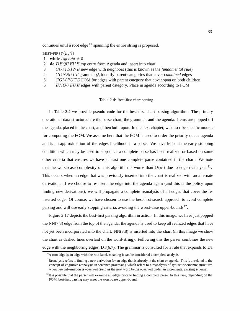
33

continues until a root edge 10 spanning the entire string is proposed.

BEST-FIRST(S,G)1 while Agenda = ∅2 do DEQUEUE top entry from Agenda and insert into chart3 COMBINE new edge with neighbors (this is known as the fundamental rule)4 CONSULT grammar G, identify parent categories that cover combined edges5 COMPUTE FOM for edges with parent category that cover span on both children6 ENQUEUE edges with parent category. Place in agenda according to FOM

Table 2.4: Best-first chart parsing.

In Table 2.4 we provide pseudo code for the best-first chart parsing algorithm. The primary

operational data structures are the parse chart, the grammar, and the agenda. Items are popped off

the agenda, placed in the chart, and then built upon. In the next chapter, we describe specific models

for computing the FOM. We assume here that the FOM is used to order the priority queue agenda

and is an approximation of the edges likelihood in a parse. We have left out the early stopping

condition which may be used to stop once a complete parse has been realized or based on some

other criteria that ensures we have at least one complete parse contained in the chart. We note

that the worst-case complexity of this algorithm is worse than O(n3) due to edge reanalysis 11.

This occurs when an edge that was previously inserted into the chart is realized with an alternate

derivation. If we choose to re-insert the edge into the agenda again (and this is the policy upon

finding new derivations), we will propagate a complete reanalysis of all edges that cover the re-

inserted edge. Of course, we have chosen to use the best-first search approach to avoid complete

parsing and will use early stopping criteria, avoiding the worst-case upper-bounds12.

Figure 2.17 depicts the best-first parsing algorithm in action. In this image, we have just popped

the NN(7,8) edge from the top of the agenda; the agenda is used to keep all realized edges that have

not yet been incorporated into the chart. NN(7,8) is inserted into the chart (in this image we show

the chart as dashed lines overlaid on the word-string). Following this the parser combines the new

edge with the neighboring edges, DT(6,7). The grammar is consulted for a rule that expands to DT10A root edge is an edge with the root label, meaning it can be considered a complete analysis.11Reanalysis refers to finding a new derivation for an edge that is already in the chart or agenda. This is unrelated to the

concept of cognitive reanalysis in sentence processing which refers to a reanalysis of syntactic/semantic structureswhen new information is observed (such as the next word being observed under an incremental parsing scheme).

12It is possible that the parser will examine all edges prior to finding a complete parse. In this case, depending on theFOM, best-first parsing may meet the worst-case upper-bound.

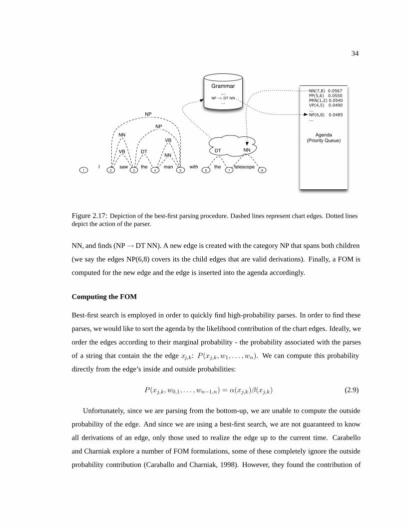
34

NN

I saw the man with the telescope1 2 3 4 5 6 7 8

DTNN

VB

VB

NN

DT

NP

NP

Agenda(Priority Queue)

NN(7,8) 0.0567PP(5,6) 0.0550PRN(1,2) 0.0540VP(4,5) 0.0490...NP(6,8) 0.0485...

Grammar...

NP -> DT NN...

Figure 2.17: Depiction of the best-first parsing procedure. Dashed lines represent chart edges. Dotted linesdepict the action of the parser.

NN, and finds (NP → DT NN). A new edge is created with the category NP that spans both children

(we say the edges NP(6,8) covers its the child edges that are valid derivations). Finally, a FOM is

computed for the new edge and the edge is inserted into the agenda accordingly.

Computing the FOM

Best-first search is employed in order to quickly find high-probability parses. In order to find these

parses, we would like to sort the agenda by the likelihood contribution of the chart edges. Ideally, we

order the edges according to their marginal probability - the probability associated with the parses

of a string that contain the the edge xj,k: P (xj,k, w1, . . . , wn). We can compute this probability

directly from the edge’s inside and outside probabilities:

P (xj,k, w0,1, . . . , wn−1,n) = α(xj,k)β(xj,k) (2.9)

Unfortunately, since we are parsing from the bottom-up, we are unable to compute the outside

probability of the edge. And since we are using a best-first search, we are not guaranteed to know

all derivations of an edge, only those used to realize the edge up to the current time. Carabello

and Charniak explore a number of FOM formulations, some of these completely ignore the outside

probability contribution (Caraballo and Charniak, 1998). However, they found the contribution of

35

an approximation to the outside probability was very useful in identifying edges that are found in

the correct parse.

One advantage of bottom-up parsing is that we can compute an approximation of an edge’s

inside probability as soon as we add it to the chart. The child edges that were combined in order to

realize the current edge each contain some partial inside probability (the inside probability for all

derivations contained in the parse chart). In order to compute the current edge’s inside probability

we take the product of the children’s current inside probabilities and the rule probability (as in the

inside recursion: Equation 2.4).

As previously mentioned, an edge may be realized more than once (due to multiple derivations)

and therefore we must add in the inside probability for each realized derivation. This can lead

to a complete recalculation of the inside probability for all edges that cover an edge with a new

derivation, nullifying the complexity gains of dynamic programming. There are two solutions to this

problem that are used in practice. The first involves delaying recalculation of the inside probability

update until it has changed sufficiently to justify propagating the changes through the parse chart.

This technique was proposed by Charniak and Carabello (1998). An alternate technique is to use the

Viterbi inside probability. The Viterbi inside probability for edge xj,l is the maximum probability

of a derivation rooted by category x spanning from j to l. We rewrite Equation 2.4 to compute the

Viterbi max probability over derivations rather than the sum:

β∗(xj,l) = maxk:k>j,k<l

r∈Ns∈N

P (x → r s)β(rj,k)β(sk,l) (2.10)

β∗(xj,j+1) = maxwj,j+1

P (x → wj, j + 1) (2.11)

In model where there probability distribution is peaked over favorable derivations, the Viterbi

inside probability should be a close approximation of the classic inside probability. We note that

if the purpose of the inside probability is to aid in the search for a max likelihood parse, then the

Viterbi probability is the correct value to be storing. However, under the PARSEVAL (Harrison et

al., 1991) labeled scoring metric, the goal is to identify the number of correct labeled brackets (the

number of correct edges). Typically, the Viterbi algorithm has been used to select a parse based

on the summed inside probabilities rather than the Viterbi inside probabilities. The result is neither

the most likely parse, nor the parse that maximizes the probability over labeled brackets. Joshua

Goodman derived an algorithm that select edges that maximize the labeled brackets criteria using

36

the inside probabilities (Goodman, 1996).

Using the Viterbi inside probability when a new derivation for an edge is introduced, the proba-

bility mass need only be propagated through the chart if it is of higher probability than the previous

Viterbi inside of the edge. This greatly simplifies the computation of the inside probability.

As for the outside probability, we are unable to compute it when parsing from the bottom up

since there may be no complete parse of the string at the time an edge is realized though the appli-

cation of the fundamental rule. Even when a complete parse exists, there may be no derivation from

a root node that reaches the current edge proposed by the parser. A number of alternative estimates

of the outside probability have been considered for parsing strings (Caraballo and Charniak, 1998).

The most widely used of these is the bitag model (Goldwater et al., 1998; Blaheta and Charniak,

1999; Charniak, 2000): a linear bigram over a sequence of part-of-speech tags. We describe this

model in the context of word-lattice in the next chapter.

Overparsing

Given we are unable to compute the optimal FOM, it is likely that the first parse found by the best-

first search will be less than optimal according to the PCFG. A technique that is used to remedy this

situation is overparsing. Overparsing is the process of allowing the parser to continue to populate

the parse chart after the first complete parse has been identified. Parsing will still be halted before

generating a complete chart, but overparsing allows for many alternate parses of the string to be

contained within the chart.

Once the parser has been halted, we compute the inside and outside probabilities for the edges

contained within the chart. We have stopped short of a complete chart, so there may be many parse

trees missing from these computations. Again, the Viterbi max score can be used rather than the

standard summed score in order to identify the max probability parse (as contained in the current

chart). We mentioned the Viterbi inside probability, a similar Viterbi outside probability is defined

as:

α∗(xj,l) = max

max i:i<jp∈Nr∈N

α(pi,l)β(ri,j)P (p → r x),

maxm:m>lp∈Nr∈N

α(pj,m)β(rl,m)P (p → x r)

(2.12)

α∗(s0,n) = 1 (2.13)

37

The product of an edge’s Viterbi inside probability and Viterbi outside probability is the probability

of the most likely parse that contains this particular edge.

In the following chapter we extend the Viterbi approximation to the computation of the outside

probability approximation and provide some insight as to why this is appropriate in our word-lattice

parsing model.

2.3.3 Using Binarized Grammars

In order to guarantee the O(n3) complexity bound for complete parsing (as is provided by a CKY

parser), the grammar being used must be binary. The decision as to how this binarization is per-

formed and where in the algorithm it is implemented is up to the model developer. An advantage

to a preprocessing binarization procedure (such as the tree transformations we presented in the pre-

vious chapter) is that any parsing algorithm that requires a binary grammar may be used without

modification. In fact the CKY parsing algorithm can be used directly on these binary grammars and

the complexity guarantee remains intact (Johnson, 1998).

In our work, we have chosen to perform binarization as a preprocessing stage. The best-first

parsing algorithm is greatly simplified by removing the internal binarization process (i.e., extending

dotted rules, etc.). As claimed in the previous chapter, the PCFG learned from the binarized trees

of the training data is the same model as the PCFG learned from the original trees13. We reiterate

that the best-first search, in particular the FOM, may perform differently depending on the type of

binarization performed.

Binarization also affects the parsing process by dividing the processing of larger rules into

smaller rules. Depending on the type of binarization used (as described in Section 2.2.4), bottom-up

parsing evaluates a rule’s right-hand-side constituents either left-to-right, right-to-left, or from the

head outward. Consider the rule (NP → NP VP PP PP). A right-binarized grammar (for bottom-up

parsing) represents this rule as: (NP → NP VP–PP–PP), (VP–PP–PP → VP PP–PP), and (PP–PP

→ PP PP). In order to discover this rule, we must first have found a PP next to a PP, then later a VP

next to the two PPs, and then an NP next to the VP. The delaying of rule evaluation is similar to the

active edge processing performed explicitly in active chart parsing algorithms. In active chart pars-

ing, a rule’s right-hand-side constituents are typically processed from left to right. We stress that

13Being the same model, distributions learned from either set of trees will assign the same probability to a tree.

38

the type of binarization applied and the choice of binarized category labels are dependent on the

parsing scheme being used (bottom-up or top-down); and that this also has an effect on the delaying

of rule evaluation.

2.3.4 A∗ Parsing and Coarse-to-fine Processing

The best-first parsing algorithm presented in the previous section searches over the space of all

parses for the input sentence. Recent work by Manning and Klein provides a means to restate the

parsing problem as a traditional graph search (Klein and Manning, 2001). In this work, they propose

using Hypergraphs to represent edges used by a chart parser on which they search using a traditional

A∗ algorithm (Klein and Manning, 2003a; Klein and Manning, 2003c).

The A∗ heuristic used by Klein and Manning is based on a factored version of the PCFG.

Although not noted in their work, this is an instance of coarse-to-fine model search (Geman and

Kochanek, 2001). In exact coarse-to-fine processing, a model is factored into a simpler model (the

coarse model). One way to do this is to define the coarse model is in terms of the conditioning states

of the fine model; we can reduce the number of conditioning events in the conditional distributions.

In the coarse model, the probability assigned to events is based on the max probability achievable

under the coarse model. We know that the maximal solution in the fine model is within the set of

superstates contained in the maximal solution of the coarse model.

We provide a simple example of coarse to fine processing for an n-gram model. We will use

a trigram as our fine model and a bigram as the coarse model. For each conditioning context in

our trigram model (each conditioning pair of words), we derive pseudo-probabilities for our bigram

model as follows:

pbg(wi|wi−1) = maxwi−1

P (wi|wi−1, wi−2) (2.14)

We use the reduced bigram model pbg to evaluate a search space (e.g., a word-lattice) exactly, finding

the most likely solution for every bigram state. When we evaluate the trigram model; at each state

we only consider the trigram states that contain the maximal bigram pbg solution. In effect, we have

reduced the number of trigram states that need to be explored by first exploring states using the

factored (coarse) model.

Best-first parsing, as used with the overparsing technique described above, can be phrased as

39

an approximate coarse-to-fine parsing model. The coarse model is not a factored model of the full

grammar model, so we have no guarantee that by using it we will find the correct solution under

the fine model. For this same reason, the FOM we describe is not an admissible A∗ search heuristic

(otherwise this would be A∗ search rather than best-first search). In practice, parsing results from

best-first PCFG parsing do as well and sometimes better than exact parsing (this is due, in part, to

the FOM containing information not available under the PCFG model). We believe the flexibility of

a heuristic function that is not required to be driven by the parsing model is well suited to our use,

where our objective is reduction in word error rate (WER) rather than obtaining high probability

parses (we hope there is a correlation between high probability parses and a low WER, but we are

not bound to this correlation).

In the work presented in this thesis, we adopt an approach proposed by Charniak (2000; 2001)

where an approximate coarse-to-fine model is used. In the following chapters, we expand on the

idea of using an impoverished grammar to perform unconstrained parsing and then reevaluating the

results using a more informed model.

Chapter 3

Word-lattice Parsing

In this chapter we describe an extension of the chart parsing algorithm which parses word-lattices.

We describe this in the context of best-first chart parsing and provide a general outline of the best-

first algorithm as applied to a word-lattice. The best-first FOM components are described in detail

as well as the motivation for the particular model we use. Specifically, we present a PCFG based

best-first word-lattice parser and in a later chapter we describe the FOM model components for

other grammars.

In order to integrate the best-first PCFG word-lattice parser into a complete language modeling

solution, we define a multi-stage parsing model based on approximate coarse-to-fine processing.

We incorporate the Charniak language model (Charniak, 2001) as a final stage of this processing

model and describe the advantages and disadvantages of such an approach.

3.1 Previous Work

There have been a number of attempts to integrate parsing with speech recognition. Many of the

solutions have focused on the concept of tightly-coupled models, meaning that the parsing model

works concurrently with the acoustic decoder. Early models attempted to integrate shift-reduce

parsing algorithms using unification-based grammars (some hand generated) (Goddeau and Zue,

1992; Goddeau, 1992). Work by Weber (1994) introduced a chart-parsing unification-based gram-

mar solution to the speech recognition decoder. A commonality of these systems is that the parser

is effectively parsing strings. As the decoder produces continuations (hypothetical next–words), the

40

41

parser extends its parse to include this next word. Due to the inefficiency of these techniques the set

of possible parses is pruned at each recognition time-frame.

The Weber parser (Weber, 1994) (also described in Kiefer et al. (2000)) extends string based

parsing technique in a similar way we do in this thesis; we highlight the differences here. First, their

parser is based on a probabilistic unification grammar and uses an active chart parsing approach

(utilizing Early dotted rules). Second, they perform a left-to-right beam search over the word-

lattices, incorporating the newly added words of the word-lattice into the parses. In order to perform

this step, they limit the number of parse analyses allowed at each point as the parser develops

analyses from left to right (i.e., they perform a beam-search). This effectively implements a greedy

search over the parses for all paths in the word-lattice. In the algorithm described they suggest that

they store all partially expanded edges that fall out of the beam, thus allowing for a global search

over all parses if the greedy beam-search is unable to find a complete parse spanning the entire

lattice.

Chappelier, et. al. describe some of the basic trade-offs in implementing word-lattice parsing

(Chappelier et al., 1999). In particular, they suggest a modification to chart-parsing that allows for

word-lattice node positions. They also describe what they call sequential–coupling of the parser

and the HMM Viterbi decoder. Sequential–coupling is the process of producing a set of n-best

candidate strings from the Viterbi decoder followed by a n-best rescoring procedure as we described

in Chapter 1. The parse scores are combined with the acoustic recognizer’s scores and might also

be combined with an n-gram language model. Using this combined parser, language model, and

acoustic model score, the best string is selected. A tight–coupling model incorporates the model

into the time-synchronous acoustic decoder, requiring left-to-right predictive models. The work

presented in this thesis lies somewhere between sequential–coupling and tight–coupling.

Recent solutions provided by Brian Roark (2001b; 2001a) and Eugene Charniak (2001) adopt

the sequential–coupling model. Roark and Charniak have both shown that a parsing-based language

model does better than the trigram language model. The Roark model uses a left-to-right left-corner

parser that has advantages in that it could work in a more tightly-coupled setting. A variation of the

Roark parser presented in Roark (2002) describes a technique for rescoring word-lattices performing

a left to right syntactic analysis of the word-lattice paths.

42

The Charniak parser is the blueprint for the word-lattice parser developed in this thesis (Char-

niak, 2000; Charniak, 2001). An implementation of approximate coarse-to-fine processing, the

parser employs a best-first PCFG active chart parser as a first-stage, utilizing overparsing to popu-

late a chart with candidate parse analyses. A second-stage model applies a sophisticated probability

model that incorporates context-dependent information. For example, conditioning contexts for rule

expansion include features such as: the syntactic category label of the parent and grandparent edges

and the head-word of the parent category (and in Charniak (2001) the grandparent or sibling cate-

gory). Conditioning information is identified for all edges contained in the chart generated by the

first-stage parser. This effectively splits the states (chart edges) of the chart, generating new states

for each unique context. The second-stage model is applied to all expanded edges and a Viterbi

parse is selected.

Ciprian Chelba et. al. propose the Structured Language Model (SLM) as a syntactically-based

language model (Chelba and Jelinek, 2000; Chelba, 2000; Xu et al., 2002; Chelba and Jelinek,

1998). Unlike the Roark and Charniak models, this is not a complete parsing model1. The SLM

builds partial parses in order to identify the head-words of the current hypothesis. Similar to the

parser we propose, the SLM parses directly from a word-lattice. The SLM proposed an admissible

A∗ heuristic that drives the search, but due to the complexity of the model, an approximation to this

heuristic is used, resulting in a best-first search.

3.2 Parsing over Word-lattices

The data structures used in chart parsing need not change in order to accommodate word-lattices. In

fact, the standard parsing algorithms apply to word-lattices, though have traditionally been applied

to strings. In some cases, there are a number of simplifications that assume the underlying structure

is a word-string rather than a word-lattice. We describe these here.

3.2.1 Linear Spans

In the CKY algorithm, the key to finding all derivations of an edge prior to processing that edge

is to process edges with smaller spans (containing fewer words) than edges with larger spans. The

1Chelba describes how the SLM can be used as a complete parser in Chelba (2000).

43

graphical structure of the word-lattice (specifically that it is a Directed Acyclic Graph) allows us to

order the nodes of the graph in such a manner that word-arcs leading into a node occur no later than

word-arcs leading into nodes further to the right (later in the sort order). This is a topological sorting

of the nodes in the graph and it allows us to use relative node positions to identify the relative order

of edge spans. This does not mean the node numbers tell us how many words are contained within

a span, only that there is a relative ordering. Standard topological sorting algorithms can be found

in texts such as (Cormen et al., 1990).

1 2 4

3

a b

c d

5f

e

g

Figure 3.1: An example of topologically sorted nodes. The sequential node number indicates one possibletopological sorting for this DAG.

Figure 3.1 is an example DAG where the nodes have been topologically sorted (node number

indicate their topologically sorted relative ordering). Given a graph with topologically sorted nodes,

we can sort the the edges of the graph such that an edge is greater than the edges it contains, we

call this a topological sorting of the edges. This sorting allows us to process in order so that all

contained edges are processed prior to the edge containing them.

We define a lessthan function that allows us to topologically sort the edges of a graph with

topologically sorted nodes, defined in Table 3.1. We use the node number to compute the size of the

edge. The size is only used in relative terms as follows:

• If the spans are of equal size, the edges either cover the exact same location or are non-

containing (smaller spans can only be contained by larger spans). In either case, we arbitrarily

define the span that starts earlier in the graph as smaller.

• If the spans are not identical, then we say the edge with a larger span contains an edge with

a smaller span. As in the previous case, if the nodes are non-containing, then the relative sort

44

LESSTHAN(e1, e2)1 span ← (e1.start − e1.end) − (e2.start − e2.end)2 if span = 03 then if e1.start > e2.start4 then // arbitrarily sort edges of same size5 return true6 else return false7 else if span < 08 then // contained span is less than containing span9 return true

10 else return false

Table 3.1: A less-than function for topologically sorted graphs

order does not matter. If the edges are containing edges, we know that a larger edge contains

an a smaller edge. We summarize the three cases where one edge contains the other:

– The edges start from the same node. Since the nodes are numbered according a topo-

logical sorting, an edge that connects to a node occurring later is guaranteed to contain

and edge connecting to an earlier node (by definition of the topological sort).

– The edges end at the same node. Same argument as above, but with the start node and

end node reversed.

– Both the start and end nodes are different. If one edge does contain the other, then that

edge must start before and after the contained edge. Due to the relative node ordering,

we know that the contained edge will have a smaller size than the containing edge.

3.2.2 Semantics of Parse Chart Edges

In standard chart parsing, the interpretation of an edge is that there is at least one derivation rooted

by the edge’s label that spans from the start node to the end node. We know that if there is more

than one derivation, all derivations are for the substring within the span. In lattice parsing, this

interpretation changes. In a word-lattice parse chart an edge indicates there is at least one derivation

rooted by the edge’s label for at least one path between the start node and the end node.

Although this is a subtle difference, it changes the way we think about computing probabilities

for edges. For example, the inside probability of an edge represents the probability associated

45

with all derivations rooted by the edge’s category label covering the edge’s span. In a word-lattice

chart this translates to the probability associated with all derivations of all paths. This change

to the semantics of a parse chart edge motivates the use of the Viterbi inside and Viterbi outside

probabilities for word-lattice parsing. In effect, we wish to avoid combining the probability of

parses over different yields (word-lattice paths).

46

3.3 Best-first Bottom-up Lattice Parsing

The pseudocode in Table 3.2 describes the bottom-up best-first chart parsing algorithm as mentioned

in the previous chapter. A few definitions should help in understanding this pseudocode:

W is the compressed word-lattice containing the acoustic recognizer scores. The word-lattice is

composed of nodes V , arcs A; and has a unique start state s, and unique end state f ;

C is the word-lattice parse chart.

G is the grammar that will be used for parsing. The grammar must be binary as described in

Section 2.2.

Q Is the priority queue parsing agenda. A chart parsing agenda is a data-structure that stores chart

edges that have been proposed by the parser. Edges are taken from the agenda and inserted

into the parse chart; following this, new edges are inserted into the agenda, via the fundamen-

tal rule. A priority queue is used for the agenda in best-first parsing. The queue is keyed off

the FOM causing high FOM edges to be at the top of the queue.

We begin with an empty agenda and initialize the chart with the word-lattice 2. The inside

probability of a terminal edge (i.e., a word-arc) is the acoustic probability P (aj,k|wj,k). We initialize

the parsing algorithm by inserting preterminal edges into the agenda. For each terminal edge we

insert edges for all preterminal rules that generate it. For those words not observed in the training

data, we insert an edge for every open-class part-of-speech 3. In order for there to be probability

associated with these unobserved preterminal rules, the preterminal distribution P (x → w), where

x ∈ T , must be smoothed (we describe the smoothing models used shortly).

Recall that the arcs of the word-lattice contain the probabilities assigned by the acoustic model

P (a|w). We incorporate these probabilities into our parsing model when adding the preterminal

nodes to the agenda. The inside probability that we actually use for preterminal nodes is:

β(xj,j′) = P (x → aj,j′) = P (x → wj,j′)P (aj,j′ |wj,j′) (3.1)

2For simplicity, the data-structure used to store the word-lattice is actual the same structure as used to store the parsechart.

3Open-class parts of speech represent the items of a vocabulary that are not fixed, such as nouns and verbs. This isopposed to the close-class words which remain relatively fixed within a language; prepositions and pronouns areexample of closed-class parts of speech.

47

INITIALIZEPARSER(C,W, G = Ω, N, s, R, Q)1 for wj,k ∈ W2 do for (x → w) ∈ R3 do FOM ← COMPUTEFOM(xj,k)4 ENQUEUE(Q, FOM, xj,k)5

LATTICEPARSE(W = (V,A, s, f), G = Ω, N, s, R)1 Q ← ∅2 C ← W3 initializeParser(C,W, R,Q, x, y, p ∈ N)4 repeat5 xj,k ← top(Q)6 DEQUEUE(Q)7 doUpdate ← INSERTEDGE(C, xj,k, Q)8 if doUpdate = true // xj,k was inserted or updated; edge subsumption9 then if xj,k = s0,end // is this a root derivation of the entire lattice?

10 then for yk,l ∈ C11 do for p ∈ N12 do if (p → x y) ∈ R13 then // combine neighbor to the right14 FOM ← COMPUTEFOM(pj,l)15 ENQUEUE(Q, FOM, pj,l)16 for yi,j ∈ C17 do for p ∈ N18 do if (p → y x) ∈ R19 then // combine neighbor to the left20 FOM ← COMPUTEFOM(pi,k)21 ENQUEUE(Q, FOM, pi,k)22 for p ∈ N, p = x23 do if (p → x) ∈ R24 then // unary rule expansion25 FOM ← COMPUTEFOM(pj,k)26 ENQUEUE(Q, FOM, pj,k)27 until xj,k = s0,end

Table 3.2: Best-first Lattice Parsing algorithm

48

As this is the base case for the inside and outside computation, we redefine the inside and outside

probabilities to be:

β(xj,k) = P (x → aj,j′ · · · ak′,k) (3.2)

α(xl,m) = P (a0,s, . . . , al′,l, xl,m, am,m′ , . . . , an′,n) (3.3)

In each iteration of the main loop, we pop the top edge xj,k from the priority queue agenda Q

and insert it into the chart. Then we apply the fundamental rule of chart parsing; we combine the

new edge with neighboring edges yi,j or yk,l (depending on which side the neighbor lies) and we

consult the grammar to ensure the rule (p → y x) or (p → x y) exists (again, depending on

which side of the edge the neighbor lies) 4; we also consider unary expansions If the rule exists,

then we create a new edge pi,k or pj,l, compute the FOM for the new parent edge, and add it to the

agenda.

The chart is constrained to contain at most one edge per unique category label, start node, and

end node. If we attempt to insert a duplicate edge, the duplicate is subsumed by the existing edge.

Subsumption of this sort occurs quite often due to the existence of alternate derivations rooted by

the same category label, covering the same subgraph.

Using the word-lattice as the parse chart allows the merging of what would be the parse charts

for each hypothesis string of the word-lattice. Structure sharing at this level comes for free from

the word-lattice parsing algorithm and offers a great reduction in duplicated effort. In effect the

chart allows for sharing information between parses of separate paths in the word-lattice. Edges are

likely to cover many paths of the lattice. Edges in an incomplete chart often cover lattice paths that

have not been explicitly considered by the parser. In the next section we describe how to determine

which chart edges are part of a complete parse.

Figure 3.2 depicts an intermediate state of the lattice-chart in our word-lattice chart parser. We

have included just a few edges to elucidate the process of structure sharing. Notice that the VP2,5

covers the sub-path that yields “man is” as well as the sub-path that yields “mans”. When there are

derivations for VP2,5 that produce both strings, the probabilities for both derivations are summarized

4If using a smoothed grammar (one that assigns probability to rule expansions not observed in the training data)we would allow all non-terminals as the parent of any pair of children. The probabilities assigned by the smoothedgrammar automatically filter out the rules that are unlikely. This would be necessary if there were coverage problems,lattice where the parser cannot find a parse. The parser described in this thesis restricts the rules to be those observedin the training data and achieves 100% coverage on the test data.

49

1

2the/0

3

duh/1.223

4man/0

5mans/0.510

6

man’s/0.916

9man/0

is/0

7

early/0

surly/0.694

early/0

10is/0

8/1.307</s>/0

surely/0

NNVB

VB

VP

VB

DT

Figure 3.2: Example of the lattice-chart

by this single VP edge (typically using the Viterbi max inside probability). A primary advantage

of this technique is the ability to share information across word-lattice sub-paths, parsing the entire

lattice without explicitly considering specific yields of the word-lattice.

The algorithm in Table 3.2 is the basic template for parsing. Typically, the parser is run beyond

the point at which the first parse is discovered. When the goal is to find a single, high probability

parse, we do this to accommodate for the heuristic FOM (i.e., the FOM may not return the parse

with highest probability according to the PCFG). When overparsing in this manner, one must define

a stopping criterion. We suggest two general type of stopping criteria:

multiplicative In multiplicative overparsing, the parser records the amount of work needed to reach

the first complete parse. In this thesis, we consider the number of agenda edge pops from

the agenda as a measure of parser work. We record the number of agenda pops needed to

complete the first parse. The parser continues to run until a multiple of the number of edges

pops to get to the first parse have been popped off the agenda.

threshold In threshold-based overparsing, the parser records a probability or FOM at the time of the

first complete parse, we call this the first-parse-FOM. We compute a minimum-FOM either by

subtracting a fixed amount of probability mass or by scaling the first-parse-FOM. The parser

is allowed to run, popping edges off of the agenda, until an FOM below the minimum-FOM

is returned.

Over-parsing techniques are generally used to make up for a FOM that does not adequately

approximate the probability of the parse according to the grammar. The hope is that by overparsing

50

we will generate enough parses that we are then able to select the optimal parse exactly using the

grammar by finding the Viterbi path.

In this thesis (and in (Charniak, 2000; Charniak, 2001)) another use for overparsing is identified.

When using the best-first chart parser as the first stage of a multi-stage, approximate coarse-to-fine

parsing model, the job of the second-stage parser is to re-evaluate the probability of the edges in the

chart. In order to provide alternate parses from which the second-stage model selects an optimal

parse, we generate a chart with a substantial number of edges5

3.3.1 Components of the Figure of Merit

There are four major components of the figure of merit as we use in this thesis. The origin of this

structure is derived from that described in (Caraballo and Charniak, 1998) and further developed in

(Goldwater et al., 1998). An ideal FOM for best-first chart parsing is an edge’s inside probability

times its outside probability.

P (xj,k,W,A) = α(xj,k)β(xj,k) (3.4)

This is the probability mass associated with all parses for the word-lattice with acoustic probabilities

A, that contain the edge xj,k (i.e., the amount of the total probability mass of all parses are parses

which use the edge xj,k. The probability here is actually the marginal probability of the edge in

parses of the acoustic word-lattice. Using the Viterbi inside and outside probability we have:

P ∗(xj,k,W,A) = α∗(xj,k)β∗(xj,k) (3.5)

In Equation 3.5, W and A are the words and acoustic date on a particular path in the word-lattice.

This path is that which maximizes

Unable to compute the (Viterbi) outside probability directly we approximate it with the follow-

ing component models.

1. A linear outside model over the parts-of-speech and words preceding and succeeding the

current edge.

5Filling the chart with all possible edges causes the second-stage parser to perform the same work as would be doneby an exhaustive parse of the lattice using the second-stage model.

51

2. A left boundary model that predicts an edge given the linear outside model preceding the

edge.

3. A right boundary model that predicts the next piece of the linear outside model given the

edge.

Combined with the estimate of the (Viterbi) inside probability, we compute the product of these

models and use the result as the FOM.

Although this description makes it seem that any four models may be combined together to

produce the FOM, specific features of the models may make for a better FOM. In particular, a linear

model that is peaked like a word n-gram may not mix well with a relatively flat model like a PCFG.

In order to accommodate differences in the model we incorporate the fudge factor described in

(Goldwater et al., 1998). This factor provides a means to adjust the FOM of an edge depending on

the number of words covered by the edge. The factor is motivated by the fact that we are mixing a

hierarchical model with a linear outside model. Edges which cover a greater span are more likely to

contain more of a hierarchy. Compare this to the linear outside model which is not effected by the

length of the span (given all models cover the same total span, the word-lattice).

3.4 PCFG Figure of Merit

In this section we develop the specific components of the figure of merit as used by our parser.

In particular we describe these components in the context of a PCFG. In Chapter 6 we describe

alternative FOM components used when parsing with different grammar models.

The components described below assume the Viterbi principle: the maximum probability of a

parse is desired rather than the sum of the probability of a set of parses. Although results from string

parsing show that using the summed inside and outside probabilities rather than the Viterbi variants,

results in higher PARSEVAL scores, we have not observed the same improvements for language

modeling. In fact, when parsing from word-lattices we are interested in finding likely parses over

particular paths in the lattice and not the probability of all parses of the lattices. Nevertheless,

we experimented with the summed version of the inside and outside probabilities in the first-stage

word-lattice parser, and found that it had no noticeable effect on accuracy in terms of word error

rate (WER).

52

The Viterbi inside and outside probabilities are the correct probabilities to compute when we

use the Viterbi algorithm to select the highest probability parse. Conveniently, we can efficiently

compute an estimate to the inside probability during parsing, making the Viterbi probabilities desir-

able. The results presented in Chapters 5, 6, and 7, are for the word-lattice parsing using the Viterbi

inside and outside probabilities.

Following is a description of the computation of the inside and outside probabilities in the con-

text of speech word-lattices. In Section 2.3 of the previous chapter the recursions used to compute

the (Viterbi) inside and outside probabilities were provided. Additional discussion on the inside and

outside probabilities as used in standard parsing can be found in most NLP texts (see (Charniak,

1993; Manning and Schutze, 1999)).

3.4.1 Computing Viterbi Inside Probabilities

The interpretation of an edge in a word-lattice parse chart is that the edge xj,k implies there is

at least one derivation rooted by category label x ∈ N over at least one path between nodes j

and k. The inside probability is redefined to account for this interpretation. First we describe the

probability mass that the inside probability represents. The inside probability for an edge, xj,l is

0 1<s>/0

2the/0

3

duh/1.223

4man/0

5mans/0.510

6

man’s/0.916

9man/0

is/0

7

early/0

surly/0.694

early/0

10is/0

8/1.307</s>/0

surely/0

NNVB

VB

VP

VB

DT

Figure 3.3: The inside probability of the VB2,5 is contained within the shaded area.

the probability of all derivations rooted by category x generating the sub-lattice Cj,l. This is the

sum of all derivations rooted by x, for all paths between nodes j and l. Figure 3.3 shows the inside

probability for the VP connected between node 2 and 5 for a partially completed chart.

β(xj,l) = P (x → Cj,l) (3.6)

53

This value is computed using the following recursion:

β(xj,l) =∑

r,s∈Nk:j<k<l

p(x → r s)β(rj,k)β(sk,l) (3.7)

+∑t∈N

p(x → t)β(tj,l)

In Equation 3.7 we assume Cj,k ⊂ Cj,l and Ck,l ⊂ Cj,l, meaning that both Cj,k and Ck,l are sub-

lattices of Cj,l. Preterminals are not explicitly expressed in this equation as they are covered by the

later term in the sum. This component covers both preterminal expansions as well as unary expan-

sions. We have included the presence of unary transitions in this equation since we have chosen to

allow these in our grammar (we use a binarized grammar, not restricted to be in Chomsky Normal

Form). By allowing these expansions, Equation 3.7 has potential to recur infinitely. In practice, we

do not compute the inside probability of unary transitions through this recursion. Instead we use the

technique described by Jelinek and Lafferty in (Jelinek and Lafferty, 1991) for computing the unary

transition probability in closed form through the use of matrix inversion. We note again, that our

experiments using the summed inside probability performed no better than using the Viterbi inside

probability. Results presented in the next chapter are for experiments using the Viterbi inside and

outside probabilities.

The Viterbi approximation assumes that we only wish to find the maximal probability of any

single path between two nodes. Applied to the computation of the inside probability, this means

that for each edge, we need only compute the probability of the best parse derivation under the edge

(each complete derivation corresponds to a single path in the sub-lattice). Rewriting Equation 3.6

gives us the Viterbi inside probability.

β(xj,l) = maxW∈Cj,l

P (x → W ) (3.8)

The Viterbi inside probability in Equation 3.8 is the probability of the max probability of a derivation

rooted by category x generating the path W , a path within the sub-lattice Cj,l. As with the summed

inside probability, we present a recursion that is used to compute the Viterbi inside probability.

β∗(xj,l)

= max

max r,s∈Nk:j<k<l

p(x → r s)β∗(rj,k)β∗(sk,l),

maxt∈N p(x → t)β∗(tj,l)

(3.9)

54

VITERBIINSIDE(C, j, k,G = Ω, N, s, R)1 for xj,k ∈ C2 do CALCBINARYINSIDE(xj,k) // compute max inside probability over binary expansions of xj,k3 ENQUEUE(A, xj,k.inside, xj,k) // push edge onto auxiliary priority queue A4 while A = ∅5 do yj,k ← top(A)6 DEQUEUE(A)7 if yj,k.inside > yj,k.inside yj,k ∈ C8 then yj,k.inside ← yj,k.inside // update inside probability in chart9 for (r → y) ∈ R, r = y

10 do if rj,k ∈ C11 then ENQUEUE(A, rj,k.inside, rj,k) // update if already in A

Table 3.3: Computation of Viterbi inside probability for unary transitions

The Viterbi inside recurrence is much like the computation of the normal inside probability,

however the sum operators have been replaced by max operators. Unlike the summed version of the

recursion, we cannot compute the Viterbi inside probability for unary transitions using a closed form

expression. In Table 3.3 we present pseudocode for the computation of Viterbi inside probabilities

of unary transitions. We use an auxiliary priority queue to store the current state of an edge’s Viterbi

inside probability. Whenever an edge’s inside probability is increased, all unary expansions that are

allowable by the grammar and are present in the chart are updated and reinserted into the priority

queue. Increases to the inside probability are percolated up through the priority queue. When the

maximal Viterbi inside probability has been computed, the priority queue will be empty.

An alternative to this approach is to precompute the maximum probability unary chain for each

pair of non-terminal categories. In the Viterbi unary transition matrix V , vr,s is the maximum

probability chain of unary rule application that rewrite r ∈ N to s ∈ N (i.e., the chain of rules from

r to s). We can use this matrix to compute the Viterbi probability for an edge in the chart.

The word-lattice parsing algorithm in Table 3.2 operates in a bottom-up manner. As previously

mentioned, this allows for an on-line calculation of the Viterbi inside probability. The function in

Table 3.4 is called from the parsing algorithm in Table 3.2 for each edge popped off the priority

queue agenda. If an edge with the same grammar category Nq and word-lattice span exists in

the chart, we compare the Viterbi inside probabilities of the new edge Nqj,k and the current chart

edge. If the new edge has a higher Viterbi inside probability, we update the inside probability of

55

INSERTEDGE(C, x, j, k, inside,Q)1 if xj,k ∈ C2 then if inside > xj,k.inside3 then xj,k.inside ← inside4 return true5 else return false6 else C ← C ∪ xj,k7 return true

Table 3.4: Online Viterbi inside calculation

the current edge. If this is a new edge, or if the Viterbi inside probability was updated, the parser

will apply the fundamental rule of chart parsing and combine this edge with its neighbors. If the

edge already existed in the chart, then many of the parent edges that are generated through the

fundamental rule application will already be in the chart. These parent edges will be placed in the

agenda with a higher probability when they were previously inserted (higher than when they were

inserted due to identical applications of the fundamental rule). As the parents are dequeued from

the agenda, they will instigate another update to the inside probability of the parent edges, and the

cycle continues. Updates to an edge’s inside probability are implicitly propagated through the chart

in this manner. An alternative is to manually propagate the inside probability through the chart

and agenda. An efficient technique to do so is described in (Caraballo and Charniak, 1998). The

technique described here is an extension of that described in (Goldwater et al., 1998).

3.4.2 Linear Outside Model

0 1<s>/0

2the/0

3

duh/1.223

4man/0

5mans/0.510

6

man’s/0.916

9man/0

is/0

7

early/0

surly/0.694

early/0

10is/0

8/1.307</s>/0

surely/0

NNVB

VB

VP

VB

DT

Figure 3.4: The outside probability of the VP2,5 is contained within the shaded areas.

56

The outside probability of an incomplete chart is depicted in the shaded region of Figure 3.4.

In a complete parse chart, the outside probability is the probability of all derivations that contain

the edge VP2,5 minus the inside probability of the edge. Clearly, in this chart there is not enough

information to compute the actual outside probability. We must consider the information we have

available in such a way that it provides an approximation of the outside probability.

a1,w1

t1

a2,w2 a3,w3 an,wn...

t2 t3 tn...

Figure 3.5: The HMM used to model the outside probability of a PCFG. This image depicts a bitag model.

In the absence of complete analyses, we use a linear outside model, an n-tag model. The n-tag

model for word-lattices is an HMM model whereby the acoustic signal and words are emitted given

a part-of-speech tag. The tag sequence is generated given the n − 1 previous tags in the sequence.

Figure 3.5 presents the bitag HMM in the standard notation for graphical models. The shaded nodes

are the observed nodes, unshaded are the unobserved. The part-of-speech tag for time position i is

represented by the random variable ti. The bitag model was proposed for string parsing (Caraballo

and Charniak, 1998; Goldwater et al., 1998) as is extended to lattices here6.

In Figure 3.6 we present a partially expanded word-lattice to contain all applicable parts-of-

speech over each word-arc. The tag-lattice is an explicit expansion of the HMM depicted in Fig-

ure 3.5. Using the tag-lattice we can compute the standard HMM forward and backward prob-

abilities as well as the Viterbi forward and backward probabilities. We have experimented with

both summed and Viterbi max version of the probabilities and found they performed equally well.

However, we should stress that the model-type used to compute the inside probability (Viterbi max

or sums) should be the same type used to compute the linear model probabilities. Otherwise, we

6When parsing strings, we have a fixed string to the left and to the right of a edge. Using the marginal edge probabilitygiven the string P (qj,k|W ) as the optimal FOM allows us to simplify the linear bitag model. This simplificationrequires the bitag distribution be computed only for those words covered by the edge. Due to the uncertainty of thepreceding and succeeding strings in a word-lattice, we are unable to make the same simplification here.

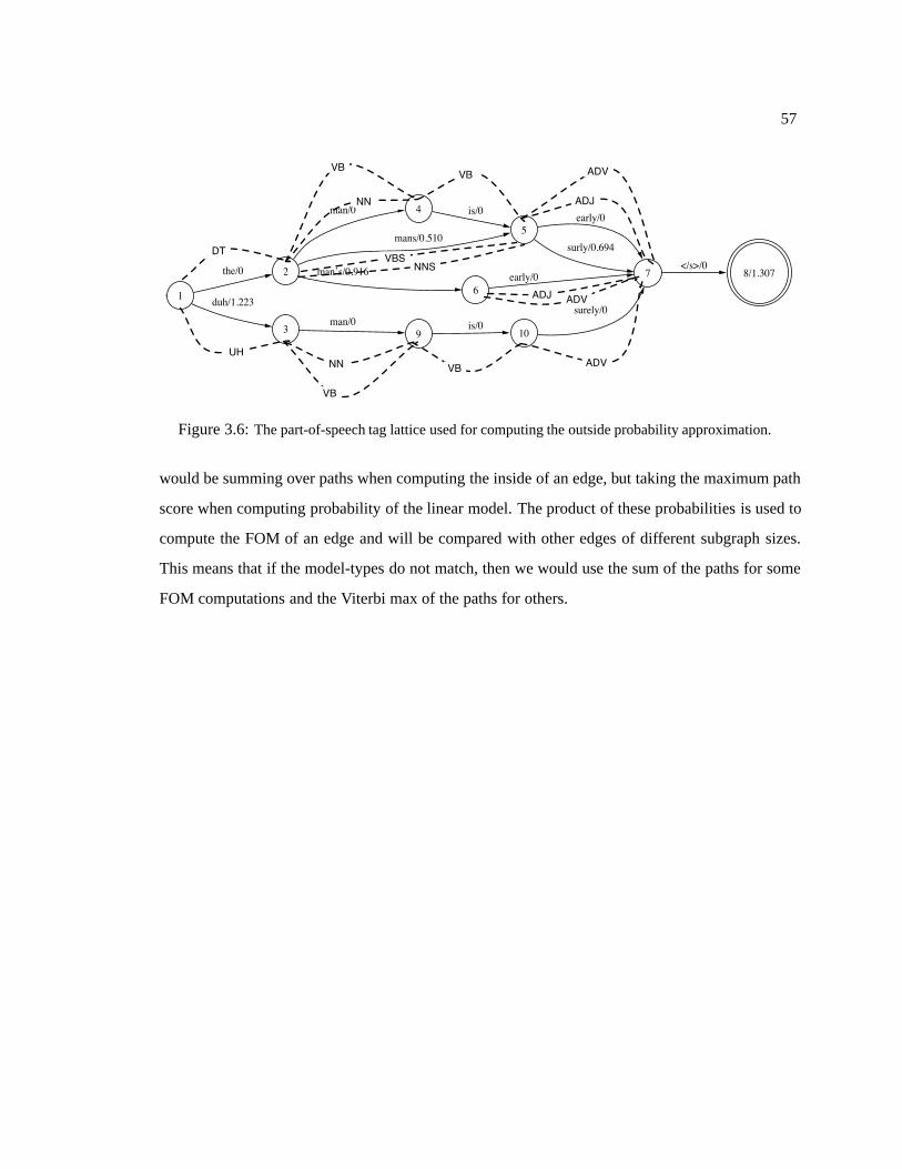
57

1

2the/0

3

duh/1.223

4man/0

5mans/0.510

6

man’s/0.916

9man/0

is/0

7

early/0

surly/0.694

early/0

10is/0

8/1.307</s>/0

surely/0

NN

VB

DT

VB

ADJ

ADV

UHNN

VB

VB ADV

NNSVBS

ADVADJ

Figure 3.6: The part-of-speech tag lattice used for computing the outside probability approximation.

would be summing over paths when computing the inside of an edge, but taking the maximum path

score when computing probability of the linear model. The product of these probabilities is used to

compute the FOM of an edge and will be compared with other edges of different subgraph sizes.

This means that if the model-types do not match, then we would use the sum of the paths for some

FOM computations and the Viterbi max of the paths for others.

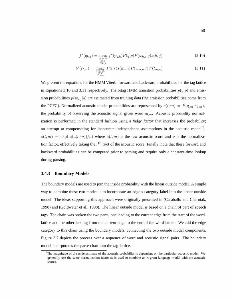
58

f∗(qh,j) = maxg:g<hp∈Twh,j

f∗(pg,h)P (q|p)P (wh,j |q)s(h, j) (3.10)

b∗(rl,m) = maxn:n>m

t∈Twm,n

P (t|r)s(m,n)P (wm,n|t)b∗(tm,n) (3.11)

We present the equations for the HMM Viterbi forward and backward probabilities for the tag lattice

in Equations 3.10 and 3.11 respectively. The bitag HMM transition probabilities p(q|p) and emis-

sion probabilities p(wh,j|q) are estimated from training data (the emission probabilities come from

the PCFG). Normalized acoustic model probabilities are represented by s(l,m) = P (al,m|wl,m),

the probability of observing the acoustic signal given word wl,m. Acoustic probability normal-

ization is performed in the standard fashion using a fudge factor that increases the probability;

an attempt at compensating for inaccurate independence assumptions in the acoustic model 7.

s(l,m) = exp(ln(a(l,m))/ν) where a(l,m) is the raw acoustic score and ν is the normaliza-

tion factor, effectively taking the νth root of the acoustic score. Finally, note that these forward and

backward probabilities can be computed prior to parsing and require only a constant-time lookup

during parsing.

3.4.3 Boundary Models

The boundary models are used to join the inside probability with the linear outside model. A simple

way to combine these two modes is to incorporate an edge’s category label into the linear outside

model. The ideas supporting this approach were originally presented in (Caraballo and Charniak,

1998) and (Goldwater et al., 1998). The linear outside model is based on a chain of part of speech

tags. The chain was broken the two parts; one leading to the current edge from the start of the word-

lattice and the other leading from the current edge to the end of the word-lattice. We add the edge

category to this chain using the boundary models, connecting the two outside model components.

Figure 3.7 depicts the process over a sequence of word and acoustic signal pairs. The boundary

model incorporates the parse chart into the tag-lattice.

7The magnitude of the underestimate of the acoustic probability is dependent on the particular acoustic model. Wegenerally use the same normalization factor as is used to combine an n-gram language model with the acousticscores.

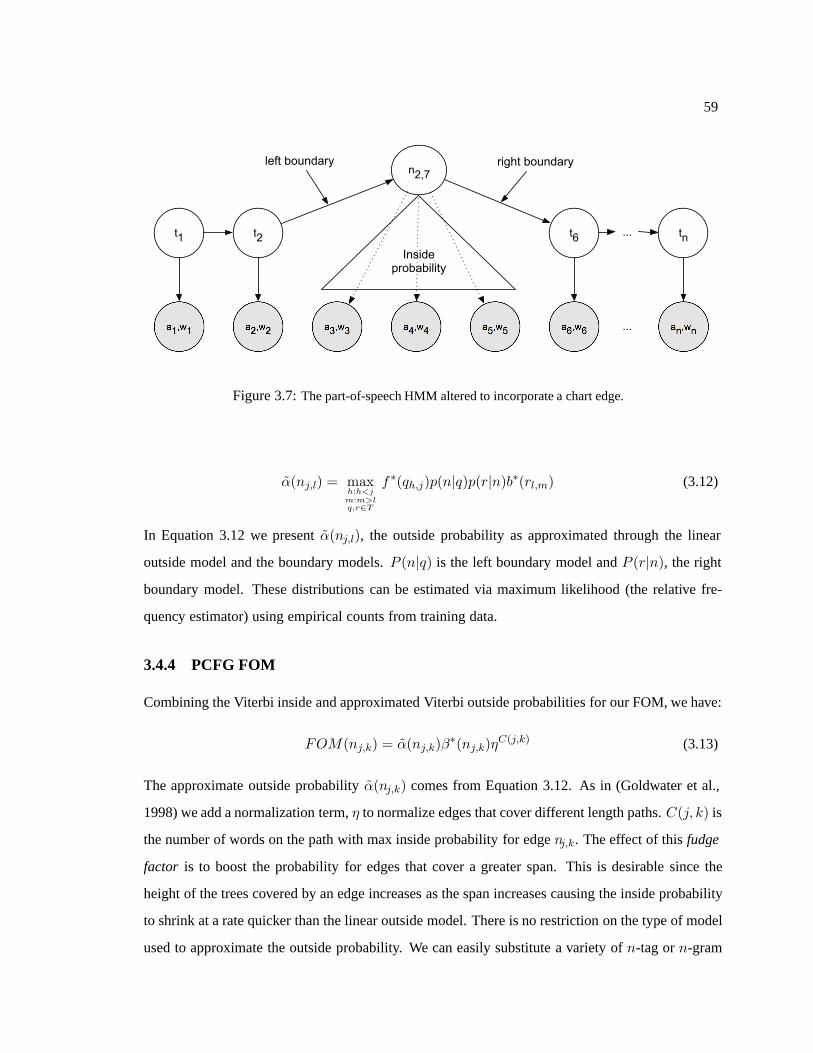
59

a1,w1

t1

a2,w2 an,wn

t2 tn

n2,7

a3,w3 a6,w6a4,w4 a5,w5 ...

...

Inside probability

t6

left boundary right boundary

Figure 3.7: The part-of-speech HMM altered to incorporate a chart edge.

α(nj,l) = maxh:h<jm:m>lq,r∈T

f∗(qh,j)p(n|q)p(r|n)b∗(rl,m) (3.12)

In Equation 3.12 we present α(nj,l), the outside probability as approximated through the linear

outside model and the boundary models. P (n|q) is the left boundary model and P (r|n), the right

boundary model. These distributions can be estimated via maximum likelihood (the relative fre-

quency estimator) using empirical counts from training data.

3.4.4 PCFG FOM

Combining the Viterbi inside and approximated Viterbi outside probabilities for our FOM, we have:

FOM(nj,k) = α(nj,k)β∗(nj,k)ηC(j,k) (3.13)

The approximate outside probability α(nj,k) comes from Equation 3.12. As in (Goldwater et al.,

1998) we add a normalization term, η to normalize edges that cover different length paths. C(j, k) is

the number of words on the path with max inside probability for edge nj,k. The effect of this fudge

factor is to boost the probability for edges that cover a greater span. This is desirable since the

height of the trees covered by an edge increases as the span increases causing the inside probability

to shrink at a rate quicker than the linear outside model. There is no restriction on the type of model

used to approximate the outside probability. We can easily substitute a variety of n-tag or n-gram

60

models in place of the bitag model presented here. As noted previously, the best-first search is very

sensitive to the mixture of these models.

Edges that are unlikely under the PCFG model (as computed from a full chart) may be assigned

a high FOM. Therefore, even when we wish to find the one most likely parse, we perform some

amount of overparsing.

3.5 Inside-Outside Pruning for Word-lattice Charts

The FOM is used to select edges during the parsing process. The FOM is only an approximation of

the Viterbi edge probability associated with the PCFG. Given a populated parse chart, we can com-

pute the Viterbi inside and outside probabilities using the actual PCFG. This allows us to compute

the actual Viterbi edge probability according to the PCFG. We have previously discussed how the

inside and Viterbi inside probabilities are computed and now discuss how the outside and Viterbi

outside probabilities are computed..

When a parse chart contains at least one complete parse (a root-edge spans from the start node

to the end node), it is possible to compute an estimate to the outside probability for edges that are

part of complete parses. An edge not covered by a complete parse has an outside probability of 0.

The outside probability of an edge in a word-lattice chart is defined as:

α(qj,l)

= P (C0,j , qj,l, Cl,n) (3.14)

(3.15)

This probability is the sum of probability mass for derivations that include edge qj,l and cover the

part of the chart lattice outside of Cj→l, minus the inside probability for edge qj,l. We use the

following recursion to compute this value:

α(qj,l)

=∑

m:m>lp,r∈N,r =q

α(pj,m)P (p → q r)β(rl,m) (3.16)

+∑i:i<j

p,r∈N

α(pi,l)P (p → r q)β(ri,j)

61

+∑p∈N

α(Npj,l)P (p → q)

As with the inside probabilities, we modify the above recursion to compute the Viterbi max outside

probability by substituting the max operator for the sum operator.

Given a partially complete chart, we compute the Viterbi outside probability and Viterbi inside

probability 8 for each edge in the chart. We take the product of these probabilities to obtain the

Viterbi max probability of the edge, word, and acoustic signal. This probability can be used to

further prune the chart of unwanted edges (those which may have been favored by the FOM, but are

given a low probability according to the grammar).

Pruning allows us to remove edges that have been added to the chart but are not likely according

to our grammar model. Due to early-stopping of the parser (i.e., overparsing), the chart may contain

edges that are not part of any complete parse. Their outside probability will be zero, and will be

pruned along with edges that fall under the edge probability threshold.

In the parsing algorithm explored in this thesis, we define the default pruning threshold to be a

function of the FOM. Recall that during parsing we are unable to compute the marginal probability

of an edge and instead use the FOM as an approximation. In order to prune the chart we use the

true probabilities, but we compute the threshold using the FOM. Since we are pruning we cannot

use the minimum marginal edge probability because this would result in no pruning. Instead we

consider the ratio between the FOM of the first complete parse and the minimum FOM of an edge

in the chart.

Let FOM1 be the the FOM for the first complete parse and FOMmin be the minimum FOM

of an edge added to the chart; we only consider the min FOM from the set of edges that have non-

zero outside probabilities. The quotient of these two values δ gives us a rough idea of the relative

probability mass allowed by overparsing.

FOM1 = FOM(s0,n) (3.17)

FOMmin = minnj,k

FOM(nj,k) (3.18)

δ =FOMmin

FOM1(3.19)

8Which we can compute on-line while parsing (see algorithm in Table 3.4) or explicitly using the recursion describedin Table 3.3 of Section 3.4.1.

62

We use delta to scale the Viterbi marginal edge probability computed for the first complete parse

p1(s0,n) (i.e., the inside probability for edge s0,n when it was first popped off the agenda).

pmin = δ × p1(s0,n) (3.20)

We prune edges from the chart that have a Viterbi marginal probability less than pmin.

At the end of this process, we have a word-lattice parse chart that contains only those edges that

have met the PCFG pruning threshold. This parse chart contains the original lattice information as

well as a set of parse edges that can be combined into parse trees for the word-lattice.

Chapter 4

Syntactic Language Modeling

The motivation behind parsing word-lattices is that by incorporating syntactic analysis in the lan-

guage model, we hope to predict word-strings that are close to the reference transcription. In (Char-

niak, 2001), Charniak shows that a syntactic language model does predict word-strings better than

n-gram models (as well as better than the SLM (Chelba and Jelinek, 2000)). In this work, we use

the Charniak syntactic language model in concert with a word-lattice parser to produce a syntactic

word-lattice language model.

Fortunately, we are able to make use of Charniak model directly by incorporating a rescoring

component of the Charniak parser. This rescoring component is capable of operating on a set of

syntactic category edges (a parse chart) by splitting the states deterministically: creating new states

which contain contextual information used by the model (head-words, parent and grandparent cate-

gories, etc.). The Charniak probability model is applied to each of new edges (split states), rescoring

each edge with the (Viterbi) inside probability according to the more sophisticated grammar (details

of the Charniak probability model can be found in (Charniak, 2001)).

We describe the integration of the Charniak rescoring component with the word-lattice chart

parser presented in the previous chapter. The model we present here is an instance of approximate

coarse-to-fine chart parsing, which we describe in the next section.

63

64

4.1 Coarse-to-fine Chart Parsing

Coarse-to-fine processing was described in Section 2.3.4 and is defined formally in (Geman and

Kochanek, 2001). In cases where exact coarse-to-fine modeling is prohibitively expensive or where

an optimal solution is preferred but not required, approximate coarse-to-fine modeling can be used.

In a two-stage coarse-to-fine model, the coarse stage is a factorization of the fine stage. Under

this factorization, the probability model for the coarse stage is determined by maximizing over

the factored terms of the fine model. An approximate alternative to this method is to estimate

the parameters of probability model for the coarse stage directly. The multi-stage parsing model

presented in this section is an instance of approximate coarse-to-fine processing, we call it coarse-

to-fine chart parsing. Although our use of such a model for direct word-lattice language modeling

is new, coarse-to-fine chart parsing for strings was introduced by Charniak in (Charniak, 2000) and

(Charniak, 2001).

1. Compress the word-lattice using WFSM compression techniques2. Compute the Viterbi forward and backward probabilities for the linear outside model3. Perform best-first parsing on the word-lattice with overparsing4. Prune the parse chart of low probability edges (according to the first-stage grammar)5. Rescore the parse edges using the Charniak context-dependent grammar6. Select the optimal parse (the word-string yield taken to be the optimal word-lattice path)

Table 4.1: Coarse-to-fine processing model.

Figure 4.1 presents the overview of the multi-stage parser we explore in this thesis. Although

Figure 4.1 only contains two stages, representing the two models, there are multiple preliminary and

intermediate processes such as word-lattice compression and inside/outside pruning. We refer to the

best-first PCFG word-lattice parser as the first-stage (the coarse model) and the Charniak context-

depended rescoring component as the second stage (the fine model). The steps of the processing

model are presented in Table 4.1.

One reason for this approach to parsing is that by producing a set of candidate edges (the parse

chart), the PCFG parser is solely responsible for search over the complete search space (the space of

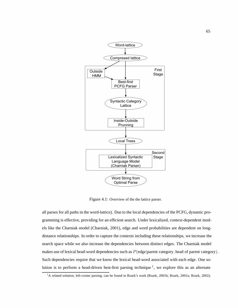
65

Compresed lattice

Outside HMM

Best-firstPCFG Parser

Syntactic CategoryLattice

Inside-OutsidePrunning

Local Trees

Lexicalized SyntacticLanguage Model(Charniak Parser)

Word String fromOptimal Parse

Word-lattice

FirstStage

SecondStage

Figure 4.1: Overview of the the lattice parser.

all parses for all paths in the word-lattice). Due to the local dependencies of the PCFG, dynamic pro-

gramming is effective, providing for an efficient search. Under lexicalized, context-dependent mod-

els like the Charniak model (Charniak, 2001), edge and word probabilities are dependent on long-

distance relationships. In order to capture the contexts including these relationships, we increase the

search space while we also increase the dependencies between distinct edges. The Charniak model

makes use of lexical head-word dependencies such as P (edge|parent category, head of parent category).

Such dependencies require that we know the lexical head-word associated with each edge. One so-

lution is to perform a head-driven best-first parsing technique 1, we explore this as an alternate

1A related solution, left-corner parsing, can be found in Roark’s work (Roark, 2001b; Roark, 2001a; Roark, 2002);

66

first-stage parsing model in a later chapter.

A disadvantage to such an approach, as with n-best rescoring techniques, is that the performance

of the second-stage model is dependent on the quality of the results of the first-stage. Since we are

performing approximate coarse-to-fine processing in both the best-first parser as well as the overall

system, we have no guarantee that the most likely parse according to the Charniak language model

will be found. For clarity, we enumerate the locations in our processing pipeline where the correct

word-lattice path might be pruned from further processing.

Best-first chart parsing During best-first chart parsing, the linear syntactic model (the bitag HMM)

combined with the Viterbi inside probability is used to select edges for the parse chart (via

the FOM-keyed agenda). When the parser is stopped (at the end of overparsing), only word-

lattice arcs which are covered by a complete parse (meaning the derivation for a parse con-

tains that particular arc) are passed on to later stages. In effect, the stopping condition controls

pruning of word-lattice arcs (and therefore word-lattice paths). A first-stage PCFG model as

described in the previous chapter only considers syntactic relationships over words, but never

considers word-to-word statistics (e.g., the bilexical statistics of a bigram are word-to-word

statistics). Therefore pruning at this stage is driven by a different model than the PCFG.

Inside/Outside pruning Other than removing those edges that are not part of complete parses (i.e.,

they have zero outside probability), this step explicitly removes category edges. If by remov-

ing these edges, we make arcs in the word-lattice unreachable (no longer part of a complete

parse), then we are pruning paths from the word-lattice as well. However, in this case we are

using the true PCFG model when pruning, but are still not using word to word statistics.

Charniak Rescoring By choosing a single parse, we are pruning all but one path in the word-

lattice (which we want to do). If the correct path exists in the pruned word-lattice prior

to this stage, and enough chart edges exist that contribute to a relatively high probability

parse, then this stage of the process should select the correct word-string. In some cases, the

conditioning information of this model may not be enough to select the correct word-string;

this is considered to be a modeling error rather than a search error.

this technique is based on a left-to-right beam search and is not a dynamic programming algorithm.

67

Throughout the presentation of experimental results we report results that evaluate the quality

of pruning as well as the quality of the complete language model. We evaluate the first-stage word-

lattice parse in terms of pruning: how close is the closest path in the pruned lattice to the reference

word-string. This is called the oracle word error rate (OWER) and is a measure of the pruning2. In

order to evaluate the overall language model we use the standard word error rate (WER) measure.

4.1.1 Second-stage Memory Constraints

Due to the extensive state-splitting performed by the Charniak language model in order to represent

all of the model dependencies, the size of the parse chart passed is limited. This means that we

cannot exhaustively populate the parse chart via overparsing. This absolute limit is determined by

the amount of available memory on the machine running the Charniak parser, in our experiments

this was usually 2 gigabytes of RAM. Limiting the size of the chart to an exact number of edges can

done by adjusting the Inside/Outside threshold.

We perform a bisection search over possible Inside/Outside threshold values for each word-

lattice parsed. The objective of this search is to generate no more than a predetermined maximum

number of chart edges 3. The effect of this constraint is that we must contain both good word-lattice

paths as well as good syntactic category edges in a limited size chart.

2The oracle WER measures the edit distance between a word-lattice and a word-string.3In fact, the Charniak language model component takes as input a forest of local-trees rather than a chart. A local-treeis a local derivation for each edges in the parse chart. The local-tree contains the parent category, children categories,and start and end nodes of each category.

Chapter 5

Speech Recognition Experiments

In this chapter we focus on an empirical evaluation of the best-first word-lattice parsing model used

as a language model for speech recognition. Much of the work on language modeling (especially

for speech recognition) has involved linear Markov models, n-grams. The results presented here

show that not only does syntactic structure help language modeling (this has been shown in Chelba

and Jelinek (2000), Charniak (2001), and Roark (2001a)), but we can efficiently parse word-lattices

directly.

There are two types of results presented in this chapter. First, we report how well the first-stage

best-first parser selects paths in the word-lattice (i.e., we measure the quality of the pruned word-

lattices). And second, we evaluate a complete language modeling system based on the best-first

parsing using the Charniak language model as a rescoring stage. These results are compared to

n-best rescoring results presented by Chelba (2000), Roark (2001a), and Charniak (2001) using the

same evaluation dataset where possible.

Analysis of the results from these speech recognition experiments suggest that there are both

modeling errors (with the Charniak language model) as well as search errors. Given the sophistica-

tion of the Charniak language model, we do not attempt to improve on this model. In the following

chapters we provide modifications to the first-stage parser in order to correct for the search errors.

68

69

5.1 Evaluation Metrics

For each set of experiments, we evaluate both the first-stage word-lattice parsing models as well as

the complete multi-stage language model. Both metrics are designed to determine how close the

results are to the correct word-string. In these experiments, the correct word-string is a transcription

of the speech utterance. We have used the standard test setting in which there is only one correct

word-string per utterance. While this may be unnaturally strict (as many word compounds and

contractions may have multiple orthographic forms), we compare our results to the results of other

techniques using the same evaluation constraints.

5.1.1 Word Error Rate

The word error rate of a string as compared to the transcription is usually computed as the minimum

edit distance. Edit distance is measured by summing the number of insertions, deletions, and substi-

tutions required to make the strings identical. A trivial O(n2) dynamic programming algorithm can

be used to compute this distance. We use the sclite scoring routine which is packaged with the NIST

Speech Recognition Scoring Toolkit (SCTK) (NIST, 1998). Given a set of reference transcriptions

and a set of hypothesized strings (the output of our language model) the sclite program computes

the minimum edit distance and returns a general word error rate (WER), as well as sentence error

rate.

5.1.2 Oracle Word Error Rate

In order to evaluate the first-stage model (the word-lattice parser) independently of the complete

language model, we provide a metric that compares a word-lattice with the reference string. The

oracle word error rate (OWER) is the minimum edit distance between a string and a word-lattice.

We are looking for the minimum edit distance between any path in the word-lattice and the reference

transcript.

The OWER can be computed efficiently by constructing a weighted finite state transducer for

both the word-lattice and the reference transcription. Arcs are added to the transducer for each word-

arc in the original word-lattice/string. These new arcs allow for a word to be deleted (translated to

an epsilon) or substituted (translated to a special symbol and then back to another word). The

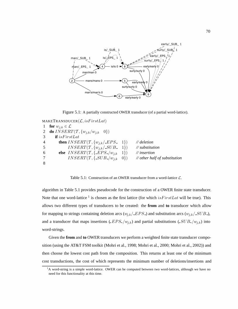
70

8

2 5

6

4

9

man/man 0

is/is 0

early/early 0

man's/man's 0

mans/mans 0

surly/surly 0

early/early 0

surly/surly 0

early/early 0man/_EPS_ 1

is/_EPS_ 1surly/_EPS_ 1

early/_EPS_ 1man/_SUB_ 1

is/_SUB_ 1 surly/_SUB_ 1

early/_SUB_ 1

Figure 5.1: A partially constructed OWER transducer (of a partial word-lattice).

MAKETRANSDUCER(L, isF irstLat)1 for wj,k ∈ L2 do INSERT (T , wj,k/wj,k 0)3 if isF irstLat4 then INSERT (T , wj,k/ EPS 1) // deletion5 INSERT (T , wj,k/ SUB 1) // substitution6 else INSERT (T , EPS /wj,k 1) // insertion7 INSERT (T , SUB /wj,k 0) // other half of substitution8

Table 5.1: Construction of an OWER transducer from a word-lattice L.

algorithm in Table 5.1 provides pseudocode for the construction of a OWER finite state transducer.

Note that one word-lattice 1 is chosen as the first lattice (for which isF irstLat will be true). This

allows two different types of transducers to be created: the from and to transducer which allow

for mapping to strings containing deletion arcs (wj,k/ EPS ) and substitution arcs (wj,k/ SUB ),

and a transducer that maps insertions ( EPS /wj,k) and partial substitutions ( SUB /wj,k) into

word-strings.

Given the from and to OWER transducers we perform a weighted finite state transducer compo-

sition (using the AT&T FSM toolkit (Mohri et al., 1998; Mohri et al., 2000; Mohri et al., 2002)) and

then choose the lowest cost path from the composition. This returns at least one of the minimum

cost transductions, the cost of which represents the minimum number of deletions/insertions and

1A word-string is a simple word-lattice. OWER can be computed between two word-lattices, although we have noneed for this functionality at this time.

71

substitutions required to transform a path in one word-lattice to a path in the other (in our case, this

is the reference transcription word-string).

5.2 Speech Data

In the following automatic speech recognition (ASR) language modeling experiments we continue

the tradition of using the NIST 1993 HUB-1 set of Wall Street Journal word-lattices (Pallett et al.,

1993). These lattices are provided by Ciprian Chelba (2000) and have been used by Chelba, Roark

(2001a), and others to evaluate the accuracy of their syntactic language modeling techniques. A few

facts about the HUB-1 word-lattices:

• The speech data comes from the ARPA Continuous Speech Recognition(CSR) corpus, Chan-

nel 1: CSR-WSJ0 (Paul and Baker, 1992); this is the high-quality ”primary” microphone data.

The speech data comes from 123 speakers reading excerpts from the Wall Street Journal text

corpus including articles from 1987, 1988, and 1989.

• Bill Byrne of Johns Hopkins University used the HTK toolkit (Young et al., 2002) with an

”out-of-the-box” training scheme to train an acoustic model using the available CSR-WSJ0

training data.

• Ciprian Chelba used this acoustic model and the trigram language model packaged with the

CSR-WSJ0 (obtained from the Linguistic Data Consortium - LDC) to generate word-lattices.

The pretrained trigram language model was trained on 45million words of Wall Street Journal

text with a 64k word vocabulary.

• 213 word-lattices were generated, corresponding the to NIST 1993 CSR HUB-1 evaluation.

The word-lattices contain the acoustic scores as well as the trigram language model scores.

One of the subtleties of using syntactic-based language models is the need for syntactic training

data. In our case, we require training data for both the first-stage PCFG word-lattice parser as well

as the second-stage lexicalized parsing model (the Charniak model). In general, a parser works

much better when trained on data from the same domain as opposed to being trained on data from a

72

different domain 2. This is a short-coming of most language-modeling techniques including n-gram

models (however the negative effect may be less severe with n-gram models). The HUB-1 speech

dataset is a set of spoken sentences from the Wall Street Journal. Conveniently, there is a large

hand-parsed dataset of Wall Street Journal articles, the Penn Wall Street Journal treebank (Marcus

et al., 1993).

When combining two models, such as the acoustic model and a language model, we need to

account for modeling characteristics that may make the probabilities of one model incompatible

with those from another. This is definitely the case when working with the acoustic model. In

order to mix our syntactic model probabilities with the acoustic probability we must normalize the

log-acoustic scores by some factor (we describe the integration of the acoustic score into the FOM

in Section 3.4.2 of Chapter 3). Throughout these experiments we use an acoustic normalization

log-scale factor of 116 (effectively the sixteenth root of the acoustic scores found in the lattices).

This parameter is found in all speech language modeling methods and is used to compensate for

inaccurate independence assumptions made in the acoustic recognition model.

Although this scale factor happens to be the same factor which minimizes the WER when mixed

with a trigram language model, we explored other values between 1 and 130 . We found that in our

experiments using the log-scale factor of 116 to be optimal when mixing with syntactic models.

5.3 Model Training

We train the PCFG word-lattice parser on the Penn Wall Street Journal treebank sections 2–21 (using

section 24 as held-out data). Prior to learning statistics for our model, we transform the tree-bank

data into speech-like data 3. Text normalization of this sort converts numerals and abbreviations

into individual tokens as they would be transcribed from speech. For example the number 125 is

converted to one hundred twenty five. The trees for the expanded strings are relabeled (CDs are

transformed into a series of NNs) and expanded to include the new tokens.

Following normalization we perform binarization and Markovization on the parse trees in the

training data. We train the PCFG from the transformed trees, resulting in a binarized, Markovized

2Recent effort in the area of parser adaptation provides hope in this area. Parser adaptation allows for a parser trainedon data from one domain to be adapted to a new domain with minimal training data from the new domain.

3We used Brian Roark’s text/speech normalization tool.

73

grammar. As described in Section 2.2 we use an aggressive Markovization strategy. We experi-

mented with the different binarization and Markovization techniques suggested in Section 2.2 and

found that they all perform relatively similar in terms of WER. We experimented with the following

PCFGs:

UnMarkovized left and right binarized grammars (described in Section 2.2.4. The labels for bina-

rized categories contained the explicit expansion of all binarized children (i.e., NN-NN-NNP-

NNP). The results for the first parse as returned by the best-first parser were slightly better

for the right-binarization 4 when run on strings of 40 words or less on f23 of the Penn WSJ

Treebank. Labeled F-measure scores at first parse were 73.3 for right-binarization and 73.0

for left-binarization (using Laplacian smoothing for the preterminal distribution).

Simple Markovization was described in Section 2.2.5 and involves forgetting all category labels

between the left and the right (the first and last child’s category label are concatenated to for

the binarized label). Labeled F-measure scores at first parse were 72.0 for right-binarization

and 72.0 for left-binarization (using Laplacian smoothing for the preterminal distribution).

The parsing score are slightly lower than without Markovization, but did not effect the overall

performance of the system (measured in WER).

Head-binarization is described in Section 2.2.4. In order to perform head-binarization we intro-

duce a head-finding procedure that is described in Chapter 6. We found a slight performance

improvement over other binarization (at first parse) but no overall effect on WER.

Maximum likelihood training of the PCFG is done using the relative frequency estimator. Pro-

vided we have enough training data, the relative frequency estimator is sufficient to learn much

of the grammar model except for the preterminal distribution, P (word|part-of-speech), which de-

scribes probability of lexical items. We smooth this distribution, reserving some probability mass

for tokens not observed in the training data. We experimented with two smoothed estimators.

5.3.1 Estimating Preterminal Probabilities

The Laplace (or Jeffrey-Perks) estimator assumes we know the size of the complete vocabulary, Ω

as well as the size of the observed vocabulary, Ω. We pretend that we have seen each word one more4Right-binarization creates right branching structures for expansions with more than two children.

74

time than it actually occurred (or a fraction of one for Jeffrey-Perks estimation).

P (x → w) =C(x → w) + 1

C(x) + |Ω| (5.1)

P (x → UNK) =1|Ω| (5.2)

Equation 5.1 is the new probability for observed data, where |Ω| is the size of the full vocabulary.

For unknown tokens, we estimate the probability by Equation 5.2. Note that we only do this for

open-class parts-of-speech. The size of the full vocabulary can be estimated using held-out data; in

a speech recognition context, the size of the acoustic recognizers vocabulary can be used (there will

never be a word in the test data that does not come from the acoustic recognizer’s vocabulary).

An alternative estimator is to actually observe how many times an unknown word is seen for

each part-of-speech in the held-out data. We also observe the number of unknown word tokens were

observed with each part-of-speech.

P (x → w) = λ(x) × P (x → w) (5.3)

P (x → UNK) = (1 − λ(x)) × 1C(x,UNK)

(5.4)

λ is the probability of observing a known word for part-of-speech x. In Equation 5.3 we discount the

observed counts, reserving probability mass for the unseen events. In Equation 5.4 we assign an un-

known word the probability of seeing an unknown word given part-of-speech Ti times the uniform

probability of observing a particular unknown word. We note that this value is approximately what

an Expectation-Maximization (EM) (Dempster et al., 1977) estimator would predict. In Chapter 6

we consider smoothed grammars, where EM is used to smooth all grammar distributions.

We found that the Laplacian estimator works as well as the suggested alternative and use it in

the following experiments.

5.3.2 Training The Charniak Parser

The second-stage parser used in these experiments is the Charniak language modeling parser (Char-

niak, 2001). The probabilistic model used in this parser uses head-words in the conditioning context

for syntactic categories, meaning that each conditional distribution in the grammar is dependent on

lexical items. Data-sparsity becomes a problem due to the number of unique contexts. We train

the Charniak model on the BLLIP99 dataset (Charniak et al., 1999); note that the BLLIP99 data is

75

produced by running the Charniak parser on a set of 30million words of Wall Street Journal data.

This version of the parser was trained on the Penn WSJ treebank (Marcus et al., 1993; Bies et al.,

1995). Training a parser on parser output has been shown to degrade the parsing accuracy but has

also been shown to increase language modeling accuracy (as measured by perplexity and WER).

Roark noted this effect in his work on parsing and language modeling (Roark, 2001b).

The BLLIP99 data comes from a set of Wall Street Journal articles that overlaps the HUB-1

dataset. For obvious reasons, we did not want to train our language model on the test data. There-

fore, we removed all overlapping sentences from the BLLIP99 corpus. We did this by identifying

the minimum edit distance between the HUB-1 reference transcriptions and the sentences in the

BLLIP corpus. Then, we manually inspected all BLLIP99 strings that were close (having an edit

distance less than 5) 5. We removed all strings that were clearly from the same source.

5.4 Experimental Setup

Most of the previous work on syntactic language modeling has made use of n-best lists. Roark

(2001a) used Chelba’s A∗ decoder to select the strings associated with the 50 best paths through

the HUB-1 word-lattices. The Chelba decoder uses the acoustic scores as well as the trigram lan-

guage model scores from the word-lattices. Rescoring an n-best list requires the processing of each

string in the list, assigning the string a language model probability and then selecting the string

that maximizes the product of the normalized acoustic model probability, and the language model

probability. Creating the n-best lists limits the maximum performance (unless the n-best selection

model is perfect).

In our results section we include results for rescoring these n-best lists. This is effectively string

parsing since the first-stage parser is given the string and converts it into a word-lattice. Structure

sharing is not possible when we parse the strings separately, as the parser works on each string in

isolation. Computationally, this is inefficient but we have observed an advantageous side-effect of

processing the strings separately; an even distribution of parser attention. In other words, when we

run the parser on the individual strings, we know that the parser considers at least a few complete

parses for each string.

5We choose an edit distance greater than 0 as some of the reference transcription strings are not exactly the same asthe strings in the automatically speech-normalized form.

76

Additionally, we experiment with n-best word-lattices. An n-best word-lattice is the sub-lattice

of the original acoustic word-lattice 6 that contains only the strings in the n-best list. N -best word-

lattices are much smaller than the acoustic word-lattices, but are also limited by the decoder used

to identify the n-best paths. Experiments on these word-lattices evaluate the effect of first-stage

pruning as well as the efficiency provided by structure sharing.

Finally, we evaluate our parser on the original acoustic word-lattices. Unlike the experiments

with the n-best lists, we do not use a language-model (the trigram language model) to preprocess

the word-lattices. In these experiments we run the PCFG word-lattice parser on the entire word-

lattice producing a set of candidates for the second-stage Charniak rescoring model. It is not until

the second stage parser that any lexical dependencies are used.

5.5 Results

Lattices OWER # arcsAcoustic Lattices 3.265 136460Acoustic 100-best 16.780 22083Acoustic 50-best 18.086 15617Chelba 50-best 7.751 11091Trigram 100-best 6.161 29998Trigram 50-best 6.417 20041

Table 5.2: Baseline Oracle WERs for HUB-1 data. # arcs is the number of arcs for the determinized,minimized word-lattice WFSMs.

Table 5.2 7 shows the baseline Oracle Word Error Rate for various manipulations of the HUB-1

dataset. The following experiments are run on the datasets in bold type; OWER for other datasets are

simply for comparison. The word-lattices in each dataset has been transformed into a compressed

WFSM prior to computing the OWER and the WFSM sizes. Measuring the cumulative size of the

dataset, the Number of Arcs field, provides a rough metric as to the size of the individual word-

lattices (although the variance is large). Acoustic n-best lists were generated by selecting the first

n highest scoring paths through the compressed lattices. Trigram n-best lists were generated in the

same way, but using the trigram language model scores in the HUB-1 dataset combined with the

6We call the original Chelba word-lattices acoustic word-lattices. These are the complete word-lattices generatedusing the acoustic model and language-model described above, but only contain scores from the acoustic model.

7WER score are presented for both Penn treebank tokenization and original lattices tokenization unless otherwisenoted. OWER scores are presented for Penn treebank tokenization only.

77

acoustic score using an acoustic normalization factor of 116 . The Chelba 50–best is the results of

Brian Roark running Ciprian Chelba’s A∗ decoder on the HUB-1 data, selecting the top 50 paths.

This results in approximately 22 strings per word-lattices (again, there is high variance).

5.5.1 Generating local-trees

The first-stage parser generates a set of candidate edges (expanded to local-trees – described in the

footnote on Page 3) which are then rescored using the Charniak language model. In Section 4.1.1

of Chapter 4 we described the memory limitation of the Charniak rescoring component. We have

found the this component can usually handle on the order of 30,000 local-trees. The number of

parse chart edges that will expand to 30,000 local-trees is dependent on the density of the chart.

Depending on the amount of over-parsing, we prune chart edges in order to generate no more than

30,000 local-trees (see Section 4.1.1).

We have explored exactly how many internal states are used by the Charniak language model

when providing 30,000 local-trees. We examined the memory requirement for one of our exper-

iments, but observed that the upper bound on the number of local-trees that can be processed in

under 2 gigabytes of RAM is around 30,000. On average, 215 expanded states were created for

each local-tree. This expands to around 6.5 million states for 30,000 local-trees; the inside proba-

bility is computed for each of these according to the Charniak model.

5.5.2 n-best Strings

In the first set of experiments, we evaluate parser-based language modeling on Chelba n-best lists.

The results give us an idea of how well we should expect to do on n-best lattice parsing. These

results are produced by parsing each string from the n-best lists individually. Strings are converted

to simple lattices (chains with word scores extracted from the acoustic lattice) and then processed

by the complete multi-stage language model, resulting in language model probabilities assigned

to the string. The string for which the combined language model and acoustic model assign the

highest probability is selected and compared to the reference transcription. Results in Table 5.3

shows the performance of string rescoring using our system. When generating charts for each of

the n-best strings, on average we generate 471 local-trees for each strings (with a maximum of

16,000). Computing the number of unique local-trees per word-lattice (combining those local trees

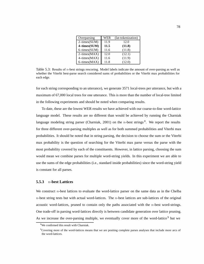
78

Overparsing WER (lat-tokenization)2–times(SUM) 11.9 12.04–times(SUM) 11.5 (11.8)6–times(SUM) 11.6 (11.8)2–times(MAX) 12.0 (12.1)4–times(MAX) 11.6 (11.9)6–times(MAX) 11.8 (12.0)

Table 5.3: Results of n-best strings rescoring. Model labels indicate the amount of over-parsing as well aswhether the Viterbi best-parse search considered sums of probabilities or the Viterbi max probabilities foreach edge.

for each string corresponding to an utterance), we generate 3571 local-trees per utterance, but with a

maximum of 67,000 local trees for one utterance. This is more than the number of local-tree limited

in the following experiments and should be noted when comparing results.

To date, these are the lowest WER results we have achieved with our coarse-to-fine word-lattice

language model. These results are no different than would be achieved by running the Charniak

language modeling string parser (Charniak, 2001) on the n-best strings 8. We report the results

for three different over-parsing multiples as well as for both summed probabilities and Viterbi max

probabilities. It should be noted that in string parsing, the decision to choose the sum or the Viterbi

max probability is the question of searching for the Viterbi max parse versus the parse with the

most probability covered by each of the constituents. However, in lattice parsing, choosing the sum

would mean we combine parses for multiple word-string yields. In this experiment we are able to

use the sums of the edge probabilities (i.e., standard inside probabilities) since the word-string yield

is constant for all parses.

5.5.3 n-best Lattices

We construct n-best lattices to evaluate the word-lattice parser on the same data as in the Chelba

n-best string tests but with actual word-lattices. The n-best lattices are sub-lattices of the original

acoustic word-lattices, pruned to contain only the paths associated with the n-best word-strings.

One trade-off in parsing word-lattices directly is between candidate generation over lattice pruning.

As we increase the over-parsing multiple, we eventually cover more of the word-lattice 9 but we

8We confirmed this result with Charniak.9Covering more of the word-lattices means that we are positing complete parses analyses that include more arcs ofthe word-lattices.

79

also generate more candidates to be rescored by the Charniak language model. At the end of over-

parsing, we prune the parse chart in order to generate at most 30,000 local-trees.

10 20 30 40 50 60 70 80 90 1008

8.2

8.4

8.6

8.8

9

9.2

Over−parsing Multiple

Ora

cle

WE

R

10 20 30 40 50 60 70 80 90 1008800

9000

9200

9400

9600

9800

10000

10200

10400

10600

Over−parsing Multiple

Num

ber

of A

rcs

Figure 5.2: Chelba n-best lattices: oracle WER and lattice size as a function of over-parsing.

In Figure 5.2 we present two graphs depicting the results after first-stage parsing: one showing

the OWER as a function of over-parsing and the other showing the size of pruned lattices as a

function of over-parsing. The y-axis in the lattice size graphs indicates the cumulative number of

WFSM arcs for all 213 first-stage pruned word-lattices, giving us a rough measure as to how much

pruning occurred. As expected, the OWER decreases as the size of the pruned lattices grow.

Overparsing a OWER # arcs # local-trees WER (lat-tokenization)14–times 9.171 8982 12.7 (12.9)50–times 8.461 10065 3188343 12.1 (12.2)100–times 8.177 10520 5229469 11.8 (12.0)

aAn average of 158 agenda pops were needed to achieve first parse on the n-best lattices.

Table 5.4: Results for various over-parsing multiples on the Chelba n-best lattices. The rightmost columnindicates the best performance of the complete system.

In Table 5.4 we present the results of the complete system for various multiples of over-parsing.

We present a few sample points showing that the WER decreases as overparsing increases. Unfortu-

nately, we found 11.8 to be the minimum total WER even with larger multiples of overparsing. Note

that these scores are better than the trigram language model scores and at 100-times over-parsing ,

close to the n-best list rescoring using the Charniak parser.

80

5.5.4 Acoustic Lattices

10 20 30 40 50 60 70 80 90 1005

5.5

6

6.5

7

7.5

8

8.5

9

Over−parsing Multiple

Ora

cle

WE

R

10 20 30 40 50 60 70 80 90 1002.5

3

3.5

4

4.5

5

5.5

6x 10

4

Over−parsing Multiple

Num

ber

of A

rcs

Figure 5.3: Acoustic lattices: oracle WER and lattice size as a function of over-parsing.

Overparsing a OWER # arcs # local–trees (# saturated) WER (lat-tokenization)14–times 8.519 28029 657047 (0) 15.7 (15.7)20–times 7.865 32938 1077634 (5) 14.8 (14.9)30–times 7.240 39010 1797814 (16) 14.3 (14.4)50–times 6.246 47170 3012479 (47) 14.0 (14.0)70–times 5.821 53106 4023065 (72) 13.1 (13.1)100–times 5.451 56525 4536720 (104) 13.1 (13.1)

aAn average of 149 agenda pops were needed to achieve first parse on the acoustic lattices.

Table 5.5: Results for various over-parsing multiples on the acoustic word-lattices. The right column indi-cates the best performance of the complete system.

Figure 5.3 and Table 5.5 present the results for the word-lattice parsing system on the acoustic

lattice. As with the n-best lattices, the first-stage parser generated at most 30,000 local-trees which

were rescored with the Charniak language model. We are able to achieve an improvement over the

trigram language model, but we do not do as well as when processing n-best lists or parsing n-best

lattices. This is not that surprising given that we are limited to a fixed number of local-trees passed

on the the second stage. With full acoustic lattices, the parser must divide the same number of parse

analyses over a much larger word-lattice. The steadily declining OWER indicates that the parser is

indeed positing edges over more of the lattice as the over-parsing multiple is increased.

Finally, note that when we increase overparsing from 70–times to 100–times, we introduce over

500,000 new local trees. The OWER improves, but the overall WER does not improve. While we

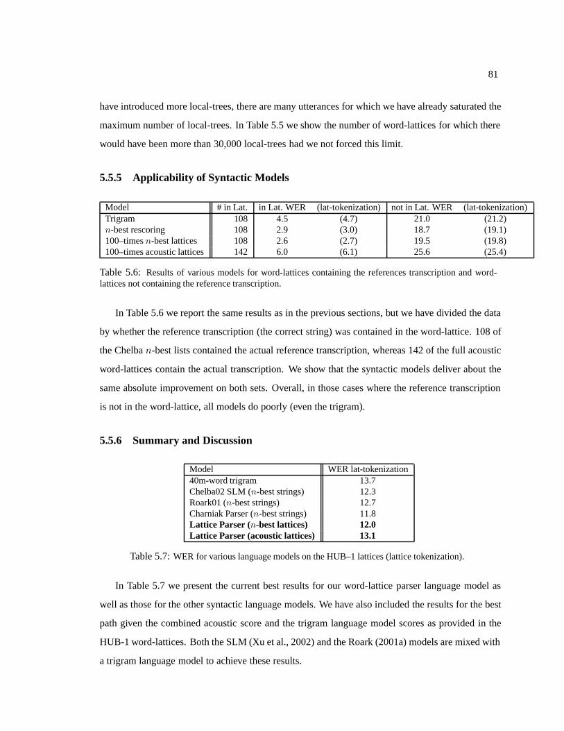
81

have introduced more local-trees, there are many utterances for which we have already saturated the

maximum number of local-trees. In Table 5.5 we show the number of word-lattices for which there

would have been more than 30,000 local-trees had we not forced this limit.

5.5.5 Applicability of Syntactic Models

Model # in Lat. in Lat. WER (lat-tokenization) not in Lat. WER (lat-tokenization)Trigram 108 4.5 (4.7) 21.0 (21.2)n-best rescoring 108 2.9 (3.0) 18.7 (19.1)100–times n-best lattices 108 2.6 (2.7) 19.5 (19.8)100–times acoustic lattices 142 6.0 (6.1) 25.6 (25.4)

Table 5.6: Results of various models for word-lattices containing the references transcription and word-lattices not containing the reference transcription.

In Table 5.6 we report the same results as in the previous sections, but we have divided the data

by whether the reference transcription (the correct string) was contained in the word-lattice. 108 of

the Chelba n-best lists contained the actual reference transcription, whereas 142 of the full acoustic

word-lattices contain the actual transcription. We show that the syntactic models deliver about the

same absolute improvement on both sets. Overall, in those cases where the reference transcription

is not in the word-lattice, all models do poorly (even the trigram).

5.5.6 Summary and Discussion

Model WER lat-tokenization40m-word trigram 13.7Chelba02 SLM (n-best strings) 12.3Roark01 (n-best strings) 12.7Charniak Parser (n-best strings) 11.8Lattice Parser (n-best lattices) 12.0Lattice Parser (acoustic lattices) 13.1

Table 5.7: WER for various language models on the HUB–1 lattices (lattice tokenization).

In Table 5.7 we present the current best results for our word-lattice parser language model as

well as those for the other syntactic language models. We have also included the results for the best

path given the combined acoustic score and the trigram language model scores as provided in the

HUB-1 word-lattices. Both the SLM (Xu et al., 2002) and the Roark (2001a) models are mixed with

a trigram language model to achieve these results.

82

These empirical results show that our best-first word-lattice parse does an adequate job at prun-

ing the word-lattices as well as positing good edges. In the following chapters we address two issues

that are revealed through these experiments. First, the best-first word-lattice parses uses a PCFG and

a Linear Syntactic Model to make the initial select of chart edges, followed by the complete PCFG

model which prunes this selection. Not only does the PCFG model only perform adequately as a

parser, but it does not model any word to word dependencies which code subtle semantic relation-

ships that help syntactic parsing (Charniak, 2000; Charniak, 2001; Roark, 2001b; Roark, 2001a;

Collins, 1999; Collins, 2003). In the following chapter, we consider alternate grammars for the

first-stage parser.

The second issue addressed is that of limited oracle word error rate. The results presented in

this chapter show that the first-stage parser is pruning correct lattice paths from the word-lattice, but

is providing adequate edges for the word-lattice paths that make it to the second stage. In Chapter 7

we present a technique that attempts to force the parser to provide edges for all paths in the word

lattice via a meta-process controlling the best-first chart parser.

Chapter 6

Alternate Grammar Models

Up to this point we have been primarily concerned with constructing a complete language modeling

solution that is driven by a best-first word-lattice parser. In this chapter, we consider alternate

grammars for use with the best-first parser. First, we consider a parent annotated grammar, known

to improve syntactic parsing results. Second, we take a look at a lexicalized PCFG, where each

constituent of a parse tree is labeled with the head-word of the phrase it covers.

We have run experiments with both of these grammars and have been unable to improve upon

the results from Chapter 5 (as measured by complete system WER). The grammars developed in

this chapter have potential to help in language modeling given either better FOM models or better

second-stage models. This development provides a basis for further research.

6.1 Parent Annotated PCFG

Previous work on syntactic parsing using PCFGs has suggested that by considering more context,

a parsing model can predict better parse trees (as measured using PARSEVAL (Harrison et al.,

1991) metric for labeled precision/recall). Johnson shows that by incorporating the parent category

label of an edge into the prediction model, labeled precision/recall improved by over 6% (absolute

improvement) (Johnson, 1998). Later work by Klein and Manning also shows that by annotating

nodes in a tree with the label of their parent category (as well as many other transformations of the

Penn Treebank category labels) performance improves (Klein and Manning, 2003b).

We have implemented a similar parent annotation transformation and have experimented with

83

84

I saw the man with the telescope

NP VP

NP

PP

S

PRP VB DT NN IN DT NN

NP

I saw the man with the telescope

NP^SVP^S

NP^VP

PP^S

S

PRP^NP VB^VP DT^NP NN^NP IN^PP DT^NP NN^NP

NP^PP

Figure 6.1: Transformation of a tree to a parent-annotated tree.

it as the grammar for the first-stage parser. Figure 6.1 depicts the parent annotation transformation.

The label of each node in a parse tree is transformed to include the label of the parent category

(always keeping only the parent category 1). Given the syntactic category of a node n in a parse tree

and the syntactic category of its parent p, we transform the category label of the child node to be

nˆ p.

As with the standard PCFG, we perform binarization and Markovization on the parent annotated

trees. We found that the maximum likelihood estimate using the relative frequency estimator was

sufficient to learn probabilities for a parent annotated PCFG. Smoothing of the preterminal distri-

bution was performed as described in Section 5.3.1 of the previous chapter. We also used the same

FOM as defined in Chapter 3, using the category labels of the parent annotated PCFG rather than

the actual category labels. In other words, the linear outside model is based on parent annotated

part-of-speech tags, as are the boundary models.

6.1.1 Experimental Results

We experimented with the parent annotated grammar on the compressed WFSM acoustic lattices

(not the n-best lattices). We used the following parameter settings for these experiments:

• We performed 100–times overparsing, requiring a minimum of 1,000 edges be popped from

the agenda.

• A maximum of 15,000 local-trees were generated from the parse chart for each word-lattice.1Klein and Manning (2003b), Charniak (2000), and Roark (2001a) incorporate grandparent category information intotheir models.

85

Overparsing a OWER # arcs # local–trees WER (lat-tokenization)100–times 5.569 48505 2042491 13.2 (13.2)

aThe parser required an average of 140 agenda pops to return a first parse, approximately the same as the with thePCFG.

Table 6.1: Results for the parent annotated PCFG on the acoustic word-lattices.

The results for the parent annotated PCFG experiment are presented in Table 6.1. Note that

while the OWER is slightly worse than the results reported in the previous section, we limited the

maximum number of local-trees to 15,000 rather than 30,000. As a result, the pruned lattices have

fewer arcs. The WER of the complete system using the parent annotated PCFG is comparable to

the results with the standard PCFG.

6.2 Lexicalized PCFG

Given that the parent annotated PCFG performed no better than a standard PCFG, we recognized

that without incorporating lexicalized rules into the grammar, the PCFG will not be able to identify

paths in the word-lattice that have better words than those in another path. Up until this point, we

were hoping that by overparsing enough, these paths would be introduced into the parse chart. In

this section, we consider a lexicalized PCFG, a PCFG that encodes the head-words of a phrase into

the nodes of the parse tree. This information is used in the grammar model in order to compute the

probability of grammar productions. There has been a substantial amount of research performed

that explores lexicalized grammar models; a few notable modes are described in Charniak (2000),

Collins (1999), and Roark (2001b).

In Figure 6.2 we present a lexicalized parse tree based on a lexicalized PCFG. The nodes of

this parse tree are similar to those in a PCFG tree; the nodes of the tree have been annotated with

additional information. In particular, we have added the head-word and the part-of-speech tag of the

head-word to each node. This information is determined based on the context of surrounding nodes

using a head-word finding algorithm (described below). Under the lexicalized PCFG, the nodes of

this tree are treated as the categories of a standard PCFG. In other words, our grammar contains

rewrite rules of the sort:

VPVB:saw

→ VBVB:saw

NPNN:man

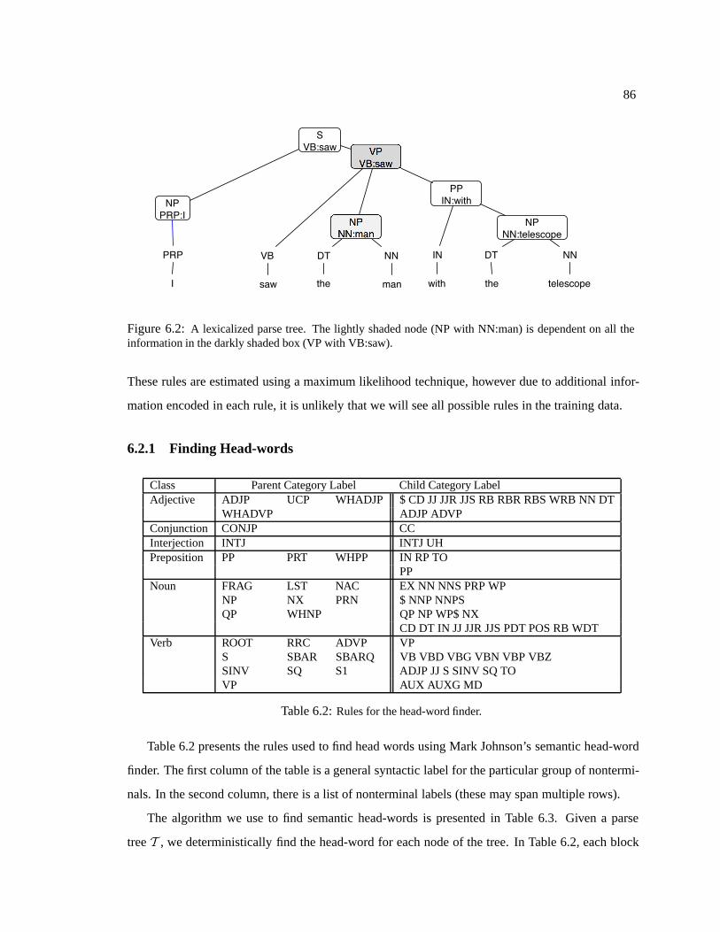
86

I saw the man with the telescope

NPPRP:I

VPVB:saw

NPNN:man

PPIN:with

SVB:saw

PRP VB DT NN IN DT NN

NPNN:telescope

Figure 6.2: A lexicalized parse tree. The lightly shaded node (NP with NN:man) is dependent on all theinformation in the darkly shaded box (VP with VB:saw).

These rules are estimated using a maximum likelihood technique, however due to additional infor-

mation encoded in each rule, it is unlikely that we will see all possible rules in the training data.

6.2.1 Finding Head-words

Class Parent Category Label Child Category LabelAdjective ADJP UCP WHADJP $ CD JJ JJR JJS RB RBR RBS WRB NN DT

WHADVP ADJP ADVPConjunction CONJP CCInterjection INTJ INTJ UHPreposition PP PRT WHPP IN RP TO

PPNoun FRAG LST NAC EX NN NNS PRP WP

NP NX PRN $ NNP NNPSQP WHNP QP NP WP$ NX

CD DT IN JJ JJR JJS PDT POS RB WDTVerb ROOT RRC ADVP VP

S SBAR SBARQ VB VBD VBG VBN VBP VBZSINV SQ S1 ADJP JJ S SINV SQ TOVP AUX AUXG MD

Table 6.2: Rules for the head-word finder.

Table 6.2 presents the rules used to find head words using Mark Johnson’s semantic head-word

finder. The first column of the table is a general syntactic label for the particular group of nontermi-

nals. In the second column, there is a list of nonterminal labels (these may span multiple rows).

The algorithm we use to find semantic head-words is presented in Table 6.3. Given a parse

tree T , we deterministically find the head-word for each node of the tree. In Table 6.2, each block

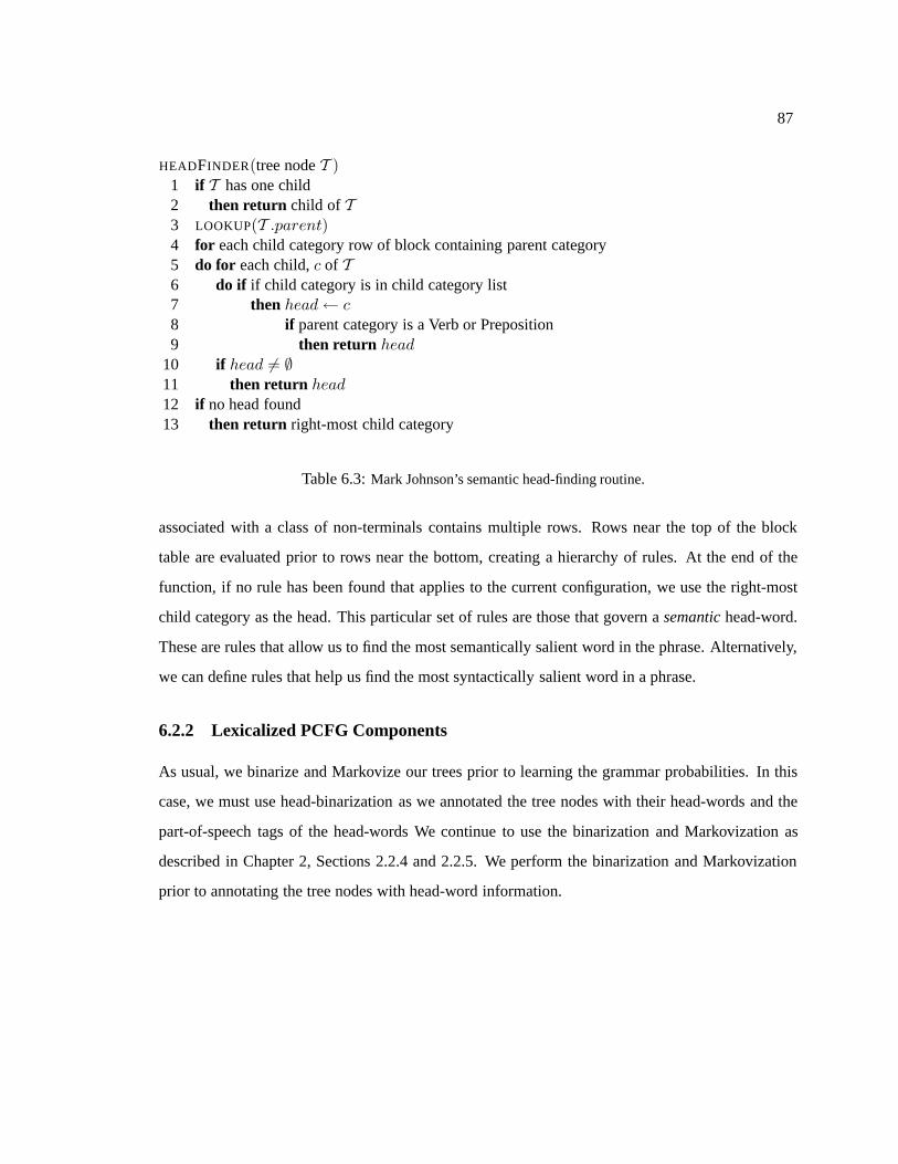
87

HEADFINDER(tree node T )1 if T has one child2 then return child of T3 LOOKUP(T .parent)4 for each child category row of block containing parent category5 do for each child, c of T6 do if if child category is in child category list7 then head ← c8 if parent category is a Verb or Preposition9 then return head

10 if head = ∅11 then return head12 if no head found13 then return right-most child category

Table 6.3: Mark Johnson’s semantic head-finding routine.

associated with a class of non-terminals contains multiple rows. Rows near the top of the block

table are evaluated prior to rows near the bottom, creating a hierarchy of rules. At the end of the

function, if no rule has been found that applies to the current configuration, we use the right-most

child category as the head. This particular set of rules are those that govern a semantic head-word.

These are rules that allow us to find the most semantically salient word in the phrase. Alternatively,

we can define rules that help us find the most syntactically salient word in a phrase.

6.2.2 Lexicalized PCFG Components

As usual, we binarize and Markovize our trees prior to learning the grammar probabilities. In this

case, we must use head-binarization as we annotated the tree nodes with their head-words and the

part-of-speech tags of the head-words We continue to use the binarization and Markovization as

described in Chapter 2, Sections 2.2.4 and 2.2.5. We perform the binarization and Markovization

prior to annotating the tree nodes with head-word information.

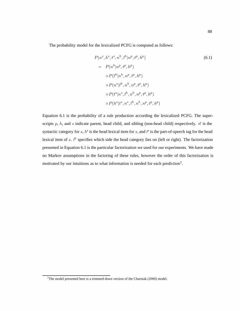
88

The probability model for the lexicalized PCFG is computed as follows:

P (ns, hs, ts, nh, lh|np, tp, hp) (6.1)

= P (nh|np, tp, hp)

×P (lh|nh, np, tp, hp)

×P (ns|lh, nh, np, tp, hp)

×P (ts|ns, lh, nh, np, tp, hp)

×P (hs|ts, ns, lh, nh, np, tp, hp)

Equation 6.1 is the probability of a rule production according the lexicalized PCFG. The super-

scripts p, h, and s indicate parent, head child, and sibling (non-head child) respectively. ns is the

syntactic category for s, hs is the head lexical item for s, and ts is the part-of-speech tag for the head

lexical item of s. lh specifies which side the head category lies on (left or right). The factorization

presented in Equation 6.1 is the particular factorization we used for our experiments. We have made

no Markov assumptions in the factoring of these rules, however the order of this factorization is

motivated by our intuitions as to what information is needed for each prediction2.

2The model presented here is a trimmed down version of the Charniak (2000) model.

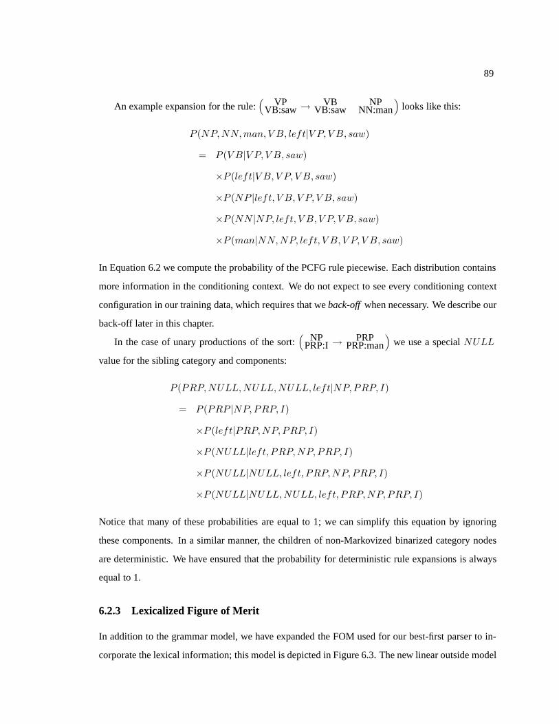
89

An example expansion for the rule:(

VPVB:saw → VB

VB:sawNP

NN:man)

looks like this:

P (NP,NN,man, V B, left|V P, V B, saw)

= P (V B|V P, V B, saw)

×P (left|V B, V P, V B, saw)

×P (NP |left, V B, V P, V B, saw)

×P (NN |NP, left, V B, V P, V B, saw)

×P (man|NN,NP, left, V B, V P, V B, saw)

In Equation 6.2 we compute the probability of the PCFG rule piecewise. Each distribution contains

more information in the conditioning context. We do not expect to see every conditioning context

configuration in our training data, which requires that we back-off when necessary. We describe our

back-off later in this chapter.

In the case of unary productions of the sort:(

NPPRP:I → PRP

PRP:man)

we use a special NULL

value for the sibling category and components:

P (PRP,NULL,NULL,NULL, left|NP,PRP, I)

= P (PRP |NP,PRP, I)

×P (left|PRP,NP,PRP, I)

×P (NULL|left, PRP,NP,PRP, I)

×P (NULL|NULL, left, PRP,NP,PRP, I)

×P (NULL|NULL,NULL, left, PRP,NP,PRP, I)

Notice that many of these probabilities are equal to 1; we can simplify this equation by ignoring

these components. In a similar manner, the children of non-Markovized binarized category nodes

are deterministic. We have ensured that the probability for deterministic rule expansions is always

equal to 1.

6.2.3 Lexicalized Figure of Merit

In addition to the grammar model, we have expanded the FOM used for our best-first parser to in-

corporate the lexical information; this model is depicted in Figure 6.3. The new linear outside model

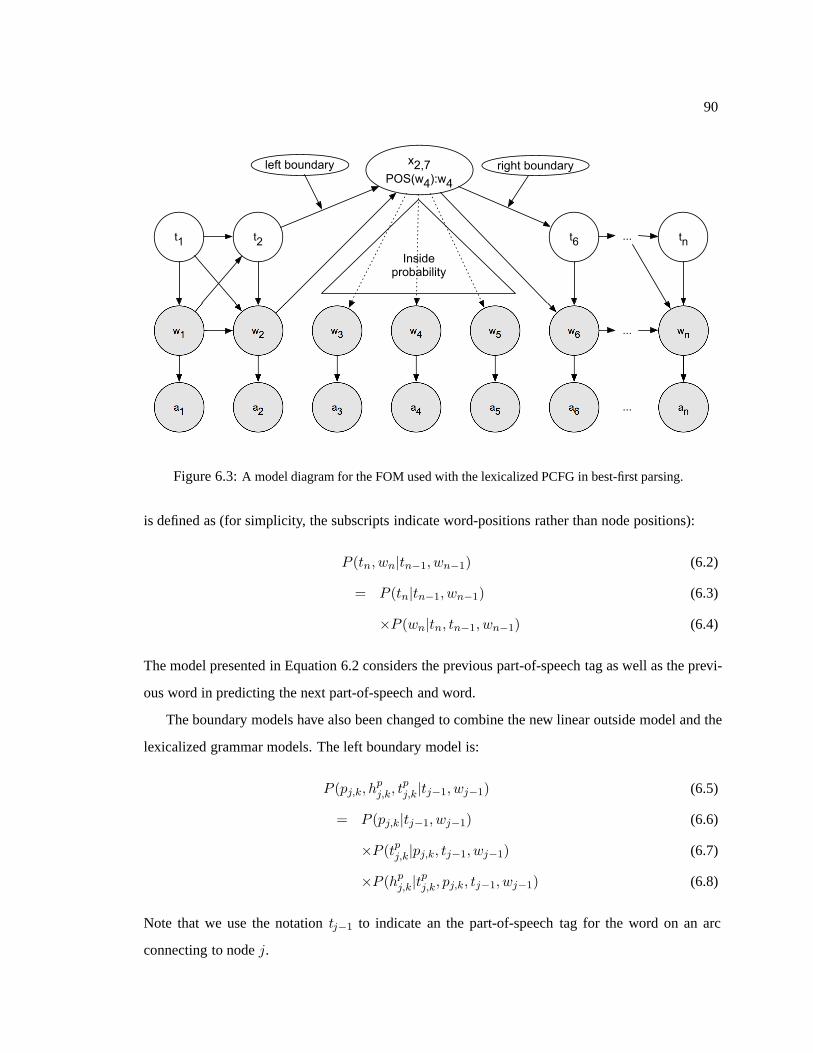
90

w1

t1

w2 wn

t2 tn

x2,7POS(w4):w4

w3 w6w4 w5 ...

...

Inside probability

t6

left boundary right boundary

a1 a2 a3 a4 a5 a6 an...

Figure 6.3: A model diagram for the FOM used with the lexicalized PCFG in best-first parsing.

is defined as (for simplicity, the subscripts indicate word-positions rather than node positions):

P (tn, wn|tn−1, wn−1) (6.2)

= P (tn|tn−1, wn−1) (6.3)

×P (wn|tn, tn−1, wn−1) (6.4)

The model presented in Equation 6.2 considers the previous part-of-speech tag as well as the previ-

ous word in predicting the next part-of-speech and word.

The boundary models have also been changed to combine the new linear outside model and the

lexicalized grammar models. The left boundary model is:

P (pj,k, hpj,k, t

pj,k|tj−1, wj−1) (6.5)

= P (pj,k|tj−1, wj−1) (6.6)

×P (tpj,k|pj,k, tj−1, wj−1) (6.7)

×P (hpj,k|t

pj,k, pj,k, tj−1, wj−1) (6.8)

Note that we use the notation tj−1 to indicate an the part-of-speech tag for the word on an arc

connecting to node j.

91

We redefine the right boundary model to be:

P (tk+1, wk+1|pj,k, tpj,k, h

pj,k) (6.9)

= P (tk+1|pj,k, tpj,k, h

pj,k) (6.10)

×P (hk+1|tk+1, pj,k, tpj,k, h

pj,k) (6.11)

We use the best-first word-lattice chart parser with these lexicalized models in the same manner

as described in Chapter 3. We found that these models worked reasonably well in parsing strings,

however not as well as typical lexicalized string parsing techniques. These models have not been

tuned for optimal string parsing, but we had hoped they would perform well for word-lattice parsing

in the context of language modeling.

6.2.4 Estimating Model Parameters

The distributions presented in the previous section have fairly complex conditioning contexts. Due

to data-sparsity, we cannot expect to observe enough of these unique contexts from a training cor-

pus such as the Penn Treebank. Therefore, the relative frequency estimator is not sufficient. The

distributions must be smoothed with a back-off model in order to assign some probability mass to

the unseen events.

The back-off model we chose was a linear back-off using deleted interpolation (Jelinek, 1997),

meaning that for each conditioning event, we removed one random variable. We backed off in order

from right to left (for the equations presented in the previous section).

Under a linear back-off model, the goal is to find a mixture of the full model and the backed-off

model that maximized the likelihood of held-out data.

P (A|B,C) = λP (A|B,C) +((1 − λ)P (A|B)

)(6.12)

In Equation 6.12 we show simple example of deleted interpolation, where the back-off model is a

version of the original model minus one conditioning variable. We use Jelinek-Mercer smoothing

(Jelinek and Mercer, 1980; Jelinek, 1997) to find the λ parameters. This is simply an instance of

the Expectation-Maximization (EM) algorithm where we are maximizing the lambda parameters

over some held-out data. The empirical distributions P are estimated from the training data using

the relative frequency estimator. We use Mark Johnson’s EM smoothing back-off tool that performs

92

Jelinek-Mercer smoothing and deleted interpolation as specified by the user. Chen bucketing is used

when tying the counts of contexts (Chen and Goodman, 1996).

6.2.5 Experimental Results

We experimented with the lexicalized PCFG and associated FOM model for use in our first-stage

best-first word-lattice parser. We trained our lexicalized PCFG on the Penn Wall Street Journal

Treebank (Marcus et al., 1993; Bies et al., 1995). We used sections 2–21 as the training set and

section 24 as our held-out data for training the smoothed back-off model.

The following parameters were used for experiments on both the n-best word-lattices as well as

the acoustic word-lattices.

• We performed 10–times and 20–times overparsing, requiring a minimum of 2,000 edges be

popped from the agenda.

• A maximum of 20,000 local-trees were generated from the parse chart for each word-lattice.

Overparsing a OWER # arcs # local–trees WER b (lat-tokenization)Trigram 7.75 11,209 N/A 13.3 (13.5)Charniak Parser (n-best strings) 7.75 91,105 2293177 11.5 (11.7)10–times 8.327 8805 606234 11.9 (12.1)20–times 8.032 9163 1065633 11.9 (12.1)

aOn average, 224 agenda pops were required to achieve first parse on the n-best lattices.b212 of the word-lattices were parsed.

Table 6.4: Results for the lexicalized PCFG on the n-best word-lattices.

Overparsing a OWER # arcs # local–trees WER b (lat-tokenization)Trigram 7.75 11,209 N/A 13.3 (13.5)Charniak Parser (n-best strings) 7.75 91,105 2293177 11.6 (11.8)10–times 6.854 27949 616604 13.7 (13.7)20–times 5.515 41192 1705425 13.1 (13.1)

aOn average, 338 agenda pops were required to achieve first parser on the acoustic lattices.b212 of the word-lattices were parsed.

Table 6.5: Results for the lexicalized PCFG on the acoustic word-lattices.

Tables 6.4 and 6.5 contain the results using the lexicalized PCFG best-first parser as the first-

stage model. We achieve almost the same accuracy (measured by both OWER and WER) as the

93

system with the standard PCFG best-first parser, but with much less overparsing (as it takes ap-

proximately double the number of agenda pops to reach first parse, 20–times overparsing here is

comparable to 40–times overparsing with the standard PCFG).

We had hoped that incorporating lexical information into the first-stage best-first parsing model

that we would do a better job at selecting word-lattice arcs. While this is true (we select good

paths with less parsing and more word-lattice pruning), this has no effect on the overall language

modeling performance of the system 3.

3The lexicalized PCFG was trained using the standard Penn Treebank, consisting of approximately 1 million wordsof parsed text. We may find that our lexicalized parser performs better when trained on a larger quantity of data.

Chapter 7

Attention Shifting

The results of the previous chapter suggest that by improving the first-stage model we cannot im-

prove the overall language modeling performance, but we can achieve the results with less com-

putational effort (i.e., fewer pops of the best-first parser agenda). In this chapter we focus on a

modification to the best-first parsing algorithm that attempts to improve efficiency by forcing the

first-stage parser to posit edges for the entire word-lattice. Ideally, such a technique would improve

the overall language modeling performance, however we observed no such improvement.

7.1 Attention Shifting Algorithm

We explore a modification to the multi-stage parsing algorithm that ensures the first stage parser

posits at least one parse for each path in the word-lattice. The idea behind this is to intermittently

shift the attention of the parser to unexplored parts of the word lattice1.

Figure 7.1 depicts the attention shifting first stage parsing procedure. A used edge is a parse

edge that has non-zero outside probability. By definition of the outside probability, used edges are

constituents that are part of a complete parse; a parse is complete if there is a root category label

(e.g., S for sentence) that spans the entire word-lattice. In order to identify used edges, we compute

the outside probabilities for each parse edge (efficiently computing the outside probability of an

edge requires that the inside probabilities have already been computed).

1The notion of attention shifting is motivated by the work on parser FOM compensation presented in (Blaheta andCharniak, 1999).

94

95

IdentifyUsed Edges

Clear Agenda/Add Edges for Unused Words

Is AgendaEmpty? no

Continue Multi-stage

Parsing

yes

PCFGWord-lattice

Parser

Figure 7.1: Attention shifting parser.

In the third step of this algorithm we clear the agenda, removing all partial analyses evaluated by

the parser. This forces the parser to abandon analyses of parts of the word-lattice for which complete

parses exist. Following this, the agenda is populated with edges corresponding to the unused words,

priming the parser to consider these words. To ensure the parser builds upon at least one of these

unused edges, we further modify the parsing algorithm:

• Only unused edges are added to the agenda.

• When building parses from the bottom up, a parse is considered complete if it connects to a

used edge.

These modifications ensure that the parser focuses on edges built upon the unused words. The

second modification ensures the parser is able to determine when it has connected an unused word

with a previously completed parse. The application of these constraints directs the attention of

the parser towards new edges that contribute to parse analyses covering unused words. We are

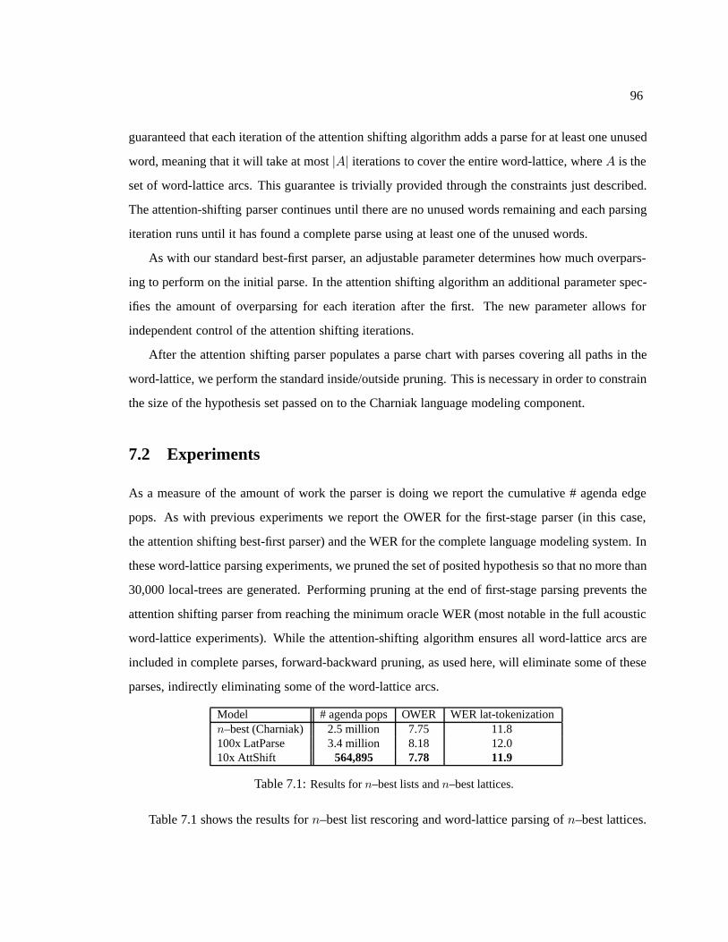
96

guaranteed that each iteration of the attention shifting algorithm adds a parse for at least one unused

word, meaning that it will take at most |A| iterations to cover the entire word-lattice, where A is the

set of word-lattice arcs. This guarantee is trivially provided through the constraints just described.

The attention-shifting parser continues until there are no unused words remaining and each parsing

iteration runs until it has found a complete parse using at least one of the unused words.

As with our standard best-first parser, an adjustable parameter determines how much overpars-

ing to perform on the initial parse. In the attention shifting algorithm an additional parameter spec-

ifies the amount of overparsing for each iteration after the first. The new parameter allows for

independent control of the attention shifting iterations.

After the attention shifting parser populates a parse chart with parses covering all paths in the

word-lattice, we perform the standard inside/outside pruning. This is necessary in order to constrain

the size of the hypothesis set passed on to the Charniak language modeling component.

7.2 Experiments

As a measure of the amount of work the parser is doing we report the cumulative # agenda edge

pops. As with previous experiments we report the OWER for the first-stage parser (in this case,

the attention shifting best-first parser) and the WER for the complete language modeling system. In

these word-lattice parsing experiments, we pruned the set of posited hypothesis so that no more than

30,000 local-trees are generated. Performing pruning at the end of first-stage parsing prevents the

attention shifting parser from reaching the minimum oracle WER (most notable in the full acoustic

word-lattice experiments). While the attention-shifting algorithm ensures all word-lattice arcs are

included in complete parses, forward-backward pruning, as used here, will eliminate some of these

parses, indirectly eliminating some of the word-lattice arcs.

Model # agenda pops OWER WER lat-tokenizationn–best (Charniak) 2.5 million 7.75 11.8100x LatParse 3.4 million 8.18 12.010x AttShift 564,895 7.78 11.9

Table 7.1: Results for n–best lists and n–best lattices.

Table 7.1 shows the results for n–best list rescoring and word-lattice parsing of n–best lattices.

97

We recreated the results of the Charniak language model parser used for rescoring in order to mea-

sure the amount of work required. We ran the first stage parser with 4-times overparsing for each

string in the n–best list. The LatParse result represents running the word-lattice parser on the n–

best lattices performing 100–times overparsing in the first stage. The AttShift model is the attention

shifting parser described in this paper. We used 10–times overparsing for both the initial parse

and each of the attention shifting iterations. When run on the n–best lattice, this model achieves a

comparable WER, while reducing the amount of parser work sixfold (as compared to the regular

word-lattice parser).

Model # edge pops OWER WER lat-tokenizationacoustic lats N/A 3.26 N/A100x LatParse 3.4 million 5.45 13.110x AttShift 1.6 million 4.17 13.1

Table 7.2: Results for acoustic lattices.

In Table 7.2 we present the results of the word-lattice parser and the attention shifting parser

when run on full acoustic lattices. While the oracle WER is reduced, we are considering almost

half as many edges as the standard word-lattice parser. The increased size of the acoustic lattices

suggests that it may not be computationally efficient to consider the entire word-lattice and that an

additional pruning phase may be necessary.

The most significant constraint of this multi-stage lattice parsing technique is that the second

stage process has a large memory requirement. While the attention shifting technique does allow

the parser to propose constituents for every path in the lattice, we prune some of these constituents

prior to performing analysis by the second stage parser.

7.3 Summary

Attention shifting is a simple technique that attempts to make word-lattice parsing more efficient. As

suggested by the results for the acoustic lattice experiments, this technique alone is not sufficient.

Solutions to improve these results include modifying the first-stage grammar by annotating the

category labels with local syntactic features as suggested in Johnson (1998) and Klein and Manning

(2003b) as well as incorporating some level of lexicalization. Improving the quality of the parses

selected by the first stage should reduce the need for generating such a large number of candidates

98

prior to pruning, improving efficiency as well as overall accuracy.

Chapter 8

Conclusion

The primary goal of this research is to provide an efficient syntactic language model that works

directly from word-lattices. Recent work by Roark shows that by moving from 100-best lists to

1000-best lists, the accuracy of an n-gram language modeling improves (Roark et al., 1994). Parsing

1000 strings per utterance is not a realistic solution, but parsing a word-lattice based on the 1000-

best lists is reasonable (we can easily move beyond 5000-best lists), hence the focus of the work in

this thesis. Unfortunately, we were not able to improve the accuracy of syntactic language modeling

by parsing full word-lattices, although we have provided an efficient solution for parsing n-best lists.

We have explored techniques for integrating parser-based language modeling into word-lattice

decoding. These techniques are based on a coarse-to-fine parsing model that uses a best-first word-

lattice parser to generate candidate parse analyses which are rescored by a sophisticated syntactic

language model, the Charniak model (Charniak, 2001).

In Chapter 3 we presented best-first word-lattice chart parsing and the general parameters for the

figure of merit that drives this algorithm. In this chapter we identify the subtle differences between

word-lattice chart parsing and that of string-based chart parsing. Specifically, we focus on a new

interpretation of a parse edge in the context of a word-lattice parsing algorithm. This interpretation

motivates two decisions through the rest of the thesis: first, that using Viterbi max estimates of the

inside, outside, and linear syntactic model is reasonable for word-lattice parsing; and second, that

structure sharing is provided automatically between the parses of different paths in the word-lattice

(defining unique word-strings). Structure sharing not only allows us to share structure between

parse analyses for different word-string yields, but it also allows for the parsing algorithm to share

99

100

parse edges among word-strings. This leads to an efficient search algorithm that simultaneously

searches the space of parse analyses as well as the space of paths in the word-lattice.

Chapter 4 presents the coarse-to-fine parsing algorithm that allows us to integrate the best-first

PCFG word-lattice parser with the Charniak language model. Due the complexity of the Charniak

model, we have to limit the size of the parse chart generated by the best-first parser. We do so by

introducing a pruning component based on the inside and outside probability of parse edges.

Empirical results are presented in Chapter 5 for the complete word-lattice language modeling

system for a speech recognition task. In order to measure the performance of our best-first word-

lattice model in isolation, we describe a technique to compute the oracle word error rate of a pruned

word-lattice. We compare the results of our model to those of competing syntactic language models

as well as the standard trigram and show that we perform as well as the Charniak model in an n-best

list rescoring setting.

The results of Chapter 5 suggest we may be able to improve search errors of the best-first word-

lattice parser. In Chapter 6 we explore two alternative grammar models for the best-first parser; a

parent annotated grammar and a lexicalized PCFG. We present experimental results of the system

with these grammars.

We also explored search inefficiencies of the best-first word-lattice parser. In Chapter 7 we

present a modification to the best-first word-lattice parsing algorithm that improves the efficiency

of the complete language-modeling system. We present experimental results for the modified algo-

rithm on the same dataset as previous experiments.

8.1 Future Directions

We see three distinct areas for future work in word-lattice parsing as presented in this thesis:

1. Further the exploration of lexicalized grammars for best-first word-lattices parsing.

2. Explore further refinements to the coarse-to-fine parsing model that allow for more explo-

ration in the first stage while still limiting the number of analyses evaluated by the final

sophisticated model.

3. Consider alternative objective functions other than those based probabilistic generative mod-

els.

101

The lexicalized model we present in Chapter 6 is one of many possible models that incorporate

lexicalization. For example, we could combine the parent annotation model and the lexicalized

model. As we consider more conditioning information, the search space becomes larger and more

complex. The goal is to find a model that we can efficiently evaluate over a larger number of parse

analyses.

As we start to think about more sophisticated lexicalized models (but less sophisticated than

the Charniak model), we realize that we may not be able to design a tractable search algorithm for

this model. As we have done with our basic model, we can use the PCFG or lexicalized PCFG

to generate a large set of analyses. We then apply an intermediate model that can handle far more

analyses than the Charniak model in order to select a subset for which we will apply the Charniak

model. This is just another stage of approximate coarse-to-fine processing.

We offer a final motivation for using a best-first parser to parse word-lattices. An advantage of

best-first parsing is that the figure of merit function, the FOM, does not have to provide an estimate

to the probability of a parse edge. In the setting explored in this thesis we use a FOM that explicitly

tries to model the maximum likelihood function, but we are actually using the FOM to pick out

parse edges that will lead to low WER word-strings. We suggest that the flexibility of the FOM

allows us to substitute in an objective function that optimizes for low WER.

Substituting alternate objective functions in place of the PCFG allows us to consider different

techniques for estimating the function. We can even explore objective functions that are not based

on probabilistic generative models such as the PCFG. In order to perform best-first search we need

a FOM that approximates the objective function. We can explore other techniques for approximat-

ing alternate objective functions, including discriminative machine learning techniques such as the

Perceptron algorithm and the Support Vector Machine.

8.2 Summary

The techniques presented here provide a framework for word-lattice parsing. We have explored a

subset of all possible grammars, FOMs, pruning conditions, and syntactic language models. What

we have shown is that it is possible to perform efficient word-lattice parsing and that we can integrate

efficient parsing with the best syntactic language model (the Charniak model). We believe the

102

techniques presented in this thesis present a complete view of best-first word-lattice parsing and

provide the basis for future research on syntactic language modeling.

References

Steve Abney. 1996. Partial parsing via finite-state cascades. Natural Language Engineering, 2(4):337–344.

J. K. Baker. 1979. Trainable grammars for speech recognition. In Proceedings of the Spring Conference of

the Acoustical Society of America, pages 547–550, Boston, MA.

Ann Bies, Mark Ferguson, Karen Katz, and Robert MacIntyre, 1995. Bracketing Guidelines for Treebank II

Style Penn Treebank Project, January.

Don Blaheta and Eugene Charniak. 1999. Automatic compensation for parser figure-of-merit flaws. In Pro-

ceedings of the 37th annual meeting of the Association for Computational Linguistics, pages 513–518.

Sharon Caraballo and Eugene Charniak. 1998. New figures of merit for best-first probabilistic chart parsing.

Computational Linguistics, 24(2):275–298, June.

J. Chappelier, M. Rajman, R. Aragues, and A. Rozenknop. 1999. Lattice parsing for speech recognition.

In Proceedings of 6me confrence sur le Traitement Automatique du Langage Naturel (TALN’99), pages

95–104.

Eugene Charniak and Keving Knight Kenji Yamada. 2003. Syntax-based language models for machine

translation. In Proceedings of MT Summit IX 2003, New Orleans.

Eugene Charniak, Don Blaheta, Niyu Ge, Keith Hall, John Hale, and Mark Johnson. 1999. BLLIP 1987–89

wsj corpus release 1. LDC corpus LDC2000T43.

Eugene Charniak. 1993. Statistical Language Learning. MIT Press.

Eugene Charniak. 1997. Statistical techniques for natural language parsing. AI Magazine, pages 33–43.

Eugene Charniak. 2000. A maximum-entropy-inspired parser. In Proceedings of the 2000 Conference of the

North American Chapter of the Association for Computational Linguistics., ACL, New Brunswick, NJ.

Eugene Charniak. 2001. Immediate-head parsing for language models. In Proceedings of the 39th Annual

Meeting of the Association for Computational Linguistics.

Ciprian Chelba and Frederick Jelinek. 1998. A study on richer syntactic dependencies for structured lan-

guage modeling. In Proceedings of the 36th Annual Meeting of the Association for Computational Lin-

guistics and 17th International Conference on Computational Linguistics, pages 225–231.

Ciprian Chelba and Frederick Jelinek. 2000. Structured language modeling. Computer Speech and Lan-

guage, 14(4):283–332.

Ciprian Chelba. 2000. Exploiting Syntactic Structure for Natural Language Modeling. Ph.D. thesis, Johns

Hopkins University.

103

Stanley F. Chen and Joshua Goodman. 1996. An empirical study of smoothing techniques for language

modeling. In Aravind Joshi and Martha Palmer, editors, Proceedings of the Thirty-Fourth Annual Meet-

ing of the Association for Computational Linguistics, pages 310–318, San Francisco. Morgan Kaufmann

Publishers.

Zhiyi Chi and Stuart Geman. 1998. Estimation of probabilistic context-free grammars. Computational Lin-

guistics, 24:299–305.

Zhiyi Chi. 1999. Statistical properties of probabilistic context-free grammars. Computational Linguistics,

25(1):132–160.

Noam Chomsky. 1970. Remarks on nominalization. In R. Jacobs and P. Rosenbaum, editors, Readings in

English Transformational Grammar. Ginn and Company, Walham, Mass.

Christopher Collins, Gerald Penn, and Bob Carpenter. 2004. Head-driven parsing for word lattices. In Pro-

ceedings of the 42nd Annual Meeting of the Association for Computational Linguistics, pages 232–239.

Michael Collins. 1999. Head-Driven Statistical Models for Natural Language Processing. Ph.D. thesis,

University of Pennsylvania.

Michael Collins. 2003. Head-driven statistical models for natural language processing. Computational Lin-

guistics, 29(4):589–637.

Thomas H. Cormen, Charles E. Leiserson, and Ronald L. Riverst. 1990. Intorduction to Algorithms. MIT

Press, Cambridge, MA.

Arthur Dempster, Nan Laird, , and Donald Rubin. 1977. Maximum likelihood from incomplete data via the

em algorithm. Royal Statistical Society, 39(1):1–38.

Stuart Geman and Mark Johnson. 2003. Probability and statistics in computational linguistics, a brief review.

In Roni Rosenfeld, Mari Ostendorf, Sanjeev Khudanpur, , and Mark Johnson, editors, Mathematical

foundations of speech and language processing. Institute for Mathematics and its Applications., pages

1–26. Springer-Verlag, New York.

Stuart Geman and K. Kochanek. 2001. Dynamic programming and the graphical representation of error-

correcting codes. IEEE Transactions on Information Theory, 47:549–568.

David Goddeau and Victor Zue. 1992. Integrating probabilistic lr parsing into speech understanding systems.

In Proceedings of ICASSP 92, San Francisco, CA.

David Goddeau. 1992. Using probabilistic shift-reduce parsing in speech recognition systems. In Proceed-

ings of ICSLP 92, Banff, Alberta, Canada.

Sharon Goldwater, Eugene Charniak, and Mark Johnson. 1998. Best-first edge-based chart parsing. In 6th

Annual Workshop for Very Large Corpora, pages 127–133.

Joshua Goodman. 1996. Parsing algorithms and metrics. In Proceedings of the 34th Annual Meeting of the

Association for Computational Linguistics, pages 177–183.

104

Joshua Goodman. 2001. A bit of progress in language modeling, extendend version. In Microsoft Research

Technical Report MSR-TR-2001-72.

Keith Hall and Mark Johnson. 2003. Language modeling using efficient best-first bottom-up parsing. In

Proceedings of IEEE Automated Speech Recognition and Understanding Workshop.

Keith Hall and Mark Johnson. 2004. Attention shifting for parsing speech. In Proceedings of the 42nd

Annual Meeting of the Association for Computational Linguistics, pages 41–47.

Zellig Harris. 1951. Methods of Structural Linguistics. University of Chicago Press, Chicago.

P. Harrison, S. Abney, D. Fleckenger, C. Gdaniec, R. Grishman, D. Hindle, B. Ingria, M. Marcus, B. San-

torini, , and T. Strzalkowski. 1991. Evaluating syntax performance of parser/grammars of english. In

Proceedings of the Workshop on Evaluating Natural Language Processing Systems, ACL.

Frederick Jelinek and John D. Lafferty. 1991. Computation of the probability of initial substring generation

by stochastic context-free grammars. Computational Linguistics, 17(3):315–323.

Frederick Jelinek and Robert L. Mercer. 1980. Interpolated estimation of markov source parameters form

sparse data. In Proceedings of the Workshop on Pattern Recognition in Practice, Amsterdam, The Neter-

lands.

Frederick Jelinek. 1997. Statistical Methods for Speech Recognition. MIT Press.

Mark Johnson. 1998. PCFG models of linguistic tree representations. Computational Linguistics, 24:617–

636.

Bernd Kiefer, Hans-Ulrich Krieger, and Mark-Jan Nederhof. 2000. Efficient and robust parsing of word

hypotheses graphs. In Wolfgang Wahlster, editor, Verbmobil: Foundations of Speech-to-Speech Transla-

tion, pages 280–295. Springer, Berlin.

Dan Klein and Christopher D. Manning. 2001. Parsing and hypergraphs. In Proceedings of the 7th Interna-

tional Workshop on Parsing Technologies (IWPT-2001).

Dan Klein and Christopher D. Manning. 2003a. A* parsing: Fast exact viterbi parse selection. In Pro-

ceedings of the 2003 Conference of the North American Chapter of the Association for Computational

Linguistics.

Dan Klein and Christopher D. Manning. 2003b. Accurate unlexicalized parsing. In Proceedings of the 41st

Meeting of the Association for Computational Linguistics (ACL-03).

Dan Klein and Christopher D. Manning. 2003c. Factored a* search for models over sequences and trees. In

Proceedings of IJCAI 2003.

Christopher D. Manning and Hinrich Schutze. 1999. Foundations of statistical natural language processing.

MIT Press.

Mitchell Marcus, Beatrice Santorini, and Mary Ann Marcinkiewicz. 1993. Building a large annotated corpus

of english: The penn treebank. Computational Linguistics, 19:313–330.

105

Mehryar Mohri and Michael Riley. 2001. A weight pushing algorithm for large vocabulary speech recogni-

tion. In Proceedings of the 7th European Conference on Speech Communication and Technology (Eu-

rospeech ’01), Aalborg, Denmark.

Mehryar Mohri, Fernando C. N. Pereira, and Michael Riley. 1998. A rational design for a weighted finite-

state transducer library. Lecture Notes in Computer Science, page 1436.

Mehryar Mohri, Fernando Pereira, and Michael Riley. 2000. The design principles of a weighted finite-state

transducer library. Theoretical Computer Science, (231):17–32.

Mehryar Mohri, Fernando C. N. Pereira, and Michael Riley. 2002. Weighted finite-state transducers in

speech recognition. Computer Speech and Language, 16(1):69–88.

NIST, 1998. Speech Recognition Scoring Toolkit (SCTK V1.2).

David S. Pallett, Jonathan G. Fiscus, William M. Fisher, John S. Garofolo, Lund Bruce A., and Mark A.

Przybocki. 1993. 1993 benchmark tests for the arpa spoken language program. NIST Report.

D. B. Paul and J. M. Baker. 1992. The design for the wall street journal-based csr corpus. In Proceedings of

the International Conference on Spoken Language Proecssing ICSLP, Banff, Alberta, Canada.

Brian Roark, Murat Saraclar, and Michael Collins. 1994. Corrective language modeling for large vocabulary

ASR with the perceptron algorithm. In Proceedings of the IEEE International Conference on Acoustics,

Speech, and Signal Processing, pages 749–752.

Brian Roark. 2001a. Probabilistic top-down parsing and language modeling. Computational Linguistics,

27(3):249–276.

Brian Edward Roark. 2001b. Robust Probabilistic Predictive Syntactic Processing: Motivations, Models,

and Applications. Ph.D. thesis, Brown University, May.

Brian Roark. 2002. Markov parsing: Lattice rescoring with a statistical parser. In Proceedings of the 40th

Annual Meeting of the Association for Computational Linguistics (ACL), pages 287–294.

Stuart Russell and Peter Norvig. 1995. Artificial Intelligence: A Modern Approach. Prentice-Hall.

Hans Weber. 1994. Time synchronous chart parsing of speech integrating unification grammars with statis-

tics. In Proceedings of the eighth Twente Workshop on Language Technologies, December.

Peng Xu, Ciprian Chelba, and Frederick Jelinek. 2002. A study on richer syntactic dependencies for struc-

tured language modeling. In Proceedings of the 40th Annual Meeting of the Association for Computa-

tional Linguistics, pages 191–198.

Steve Young, Gunnar Evermann, Dan Kershaw, Gareth Moore, Julian Odell, Dave Ollason, Dan Povey,

Valtcho Valtchev, and Phil Woodland. 2002. The HTK Book. Cambridge University Engineering De-

partment, http://htk.eng.cam.ac.uk/docs/docs.shtml.

Daniel H. Younger. 1967. Recognition and parsing of context-free languages in time n 3. Information and

Control, 10:189–208.