Best Practice Modeling for Equity Structured Products · OUTLINE • Description of Models and their properties. • Results of Market Calibration. • Model Prices for Equity Structured

Best Practice Modeling for

Equity Structured Products

Dilip B. MadanRobert H. Smith School of Business

University of Maryland

CARISMA Event

7 City Learning

London

June 28 2007

OUTLINE

• Description of Models and their properties.

• Results of Market Calibration.

• Model Prices for Equity Structured Products.

• Spot and Option Risks to be Hedged in EquityStructured Products.

Description of Models and their Properties

• There are two broad classes of models used incalibrating the prices of options and on occasion,

forward starting options.

— One dimensional Markov models in which the

future evolution of the stock price at any time

depends on just the level of the current stock

price.

— Stochastic volatility models in which the volatil-

ity of stock has an independent component to

its evolution.

• The sample paths of prices may be continuous,continuous with occasional jumps in the price, or

purely discontinuous in that the uncertain com-

ponent is just the sum of all the discrete jumps

or moves.

— The continuous sample path models may be

seen as ones with an uncertain component

made up of infinitesimally small jumps.

• I will describe two one dimensional Markov mod-els, one that has continuous sample paths and the

other that is purely discontinuous. These are

— (LV ) The Local Volatility Model.

— (LL) The Local Levy Model.

• For the class of stochastic volatility models, I willdescribe the structure of 9 models. These are

— (HSV ) Heston Stochastic Volatility.

— (SV J) Merton Jump Diffusion with stochas-

tic volatility.

— (V GSA) Stochastic Volatility for Levy Processes.

— (SV DNE) Jump Diffusion with stochastic volatil-

ity and Double Negative Exponential Jumps.

— (SV V G) Jump Diffusion with stochastic volatil-

ity and Variance Gamma Jumps.

— (SV CGMY ) Jump Diffusion with stochastic

volatility and CGMY jumps.

— Stochastic volatility and stochastic jump ar-

rival for DNE,V G,CGMY or the models

∗ (SV ADNE), (SV AV G), (SV ACGMY ).

Local Volatility Model

• For all models we focus attention on the uncer-tainty, the drift or growth rate for pricing purposes

is the interest rate net of the dividend yield or the

net finance cost.

• The local uncertainty for a local volatility model isa zero mean Normally distributed random variable

with a variance that is an unknown function of the

stock price and calendar time.

— The variance is not constant as it is for Black

Scholes.

∗ But is given by the functionσ2(S, t)

if at time t the stock price is at level S.

• Dupire (1994) showed how one may recover thisfunction from the prices of traded call options of

all strikes K and maturities T.

• Specifically we have the formula in terms of callprices C(K,T ) that

σ2(K,T ) =2

K2CKK(CT + ηC + (r − η)KCK) .

• Different strategies are used for interpolating callprices across the strike and maturity ranges to

recover the local volatilities.

• A well known problem with local volatility is that

the market skew is calibrated completely by the

dependence of volatility on the spot price.

— As a result we get a sharp dependence with

the consequence that for low spots there is

a substantial probability of getting to a high

spot but not the other way around,

∗ So over time, volatilities and skews drop aswe observed earlier.

• This makes the model unsuited for cliquet struc-tures that are highly dependent on forward skews.

Local Levy Models

• Recently, Carr, Geman, Madan and Yor (2004)generalized local volatility to allow for local un-

certainty to be modeled by a Levy distribution

that can accomodate asymmetry directly by al-

lowing for the arrival rate of negative moves at a

higher rate than the correspondingly sized posi-

tive move.

• In this way some of the skew is hard wired into

the process with a residual part being modeled

by the dependence of local quadratic variation on

the spot.

• In a local Levy model, the local variance is mod-eled by the speed at which the Levy process is run-

ning and we have a local space dependent speed

function

a(S, t).

• Carr, Geman, Madan and Yor (2004) show how

to recover this speed function from traded option

prices.

• Specifically we have the formula

•a(K,T ) =

b (ln(K), T )

K2CKK

where we call the function b(ln(K), T ) the log

speed function and it may be recovered from op-

tion prices written as functions of the log strike

c(k, T ) = C(ek, T ).

• using

Z ∞−∞

b(y)ψe(k − y)dy = (cT + ηc+ (r − η) ck)

where the function ψe is known in terms of the ar-

rival rate of jumps of the localizing Levy process.

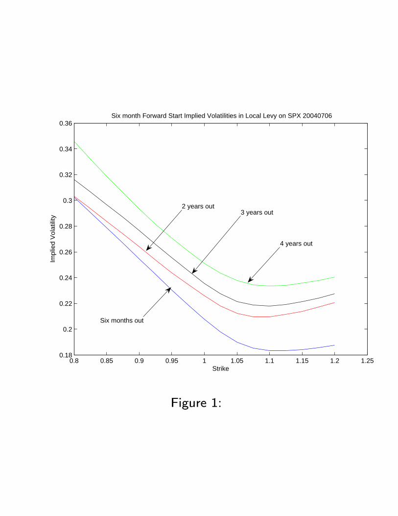
• An implementation of local Levy on SPX for

20040706 shows that forward volatilities and skews

maintain their levels and shapes as evidenced by

the following forward implied volatility curves.

Heston Stochastic Volatility

• Stochastic volatility models are important for man-aging the exposure to volatility of volatility forproduts with volgamma. The most basic stochas-tic volatility is the Heston model in which the lo-cal variance of the stock is mean reverting with

long term variance = η

mean reversion rate = κ

— and local variance is itself stochastic with alocal volatility of

vol of vol = λ

— with a correlation between the volatility andstock movements of

correlation = ρ.

— the initial level of variance is also to be esti-mated

initial volatilty = v0

0.8 0.85 0.9 0.95 1 1.05 1.1 1.15 1.2 1.250.18

0.2

0.22

0.24

0.26

0.28

0.3

0.32

0.34

0.36Six month Forward Start Implied Volatilities in Local Levy on SPX 20040706

Strike

Impl

ied

Vol

atili

ty

Six months out

2 years out3 years out

4 years out

Figure 1:

• The sample paths are continuous and in this ab-sence of jumps the shorter maturity options are

poorly calibrated.

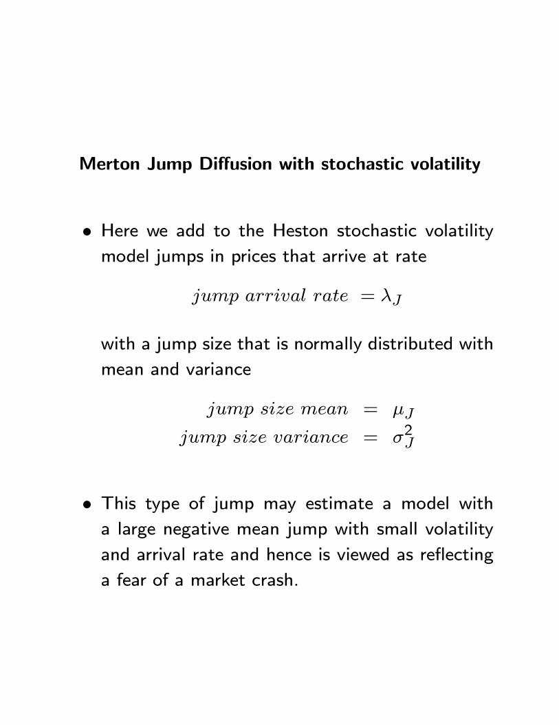
Merton Jump Diffusion with stochastic volatility

• Here we add to the Heston stochastic volatilitymodel jumps in prices that arrive at rate

jump arrival rate = λJ

with a jump size that is normally distributed with

mean and variance

jump size mean = µJ

jump size variance = σ2J

• This type of jump may estimate a model witha large negative mean jump with small volatility

and arrival rate and hence is viewed as reflecting

a fear of a market crash.

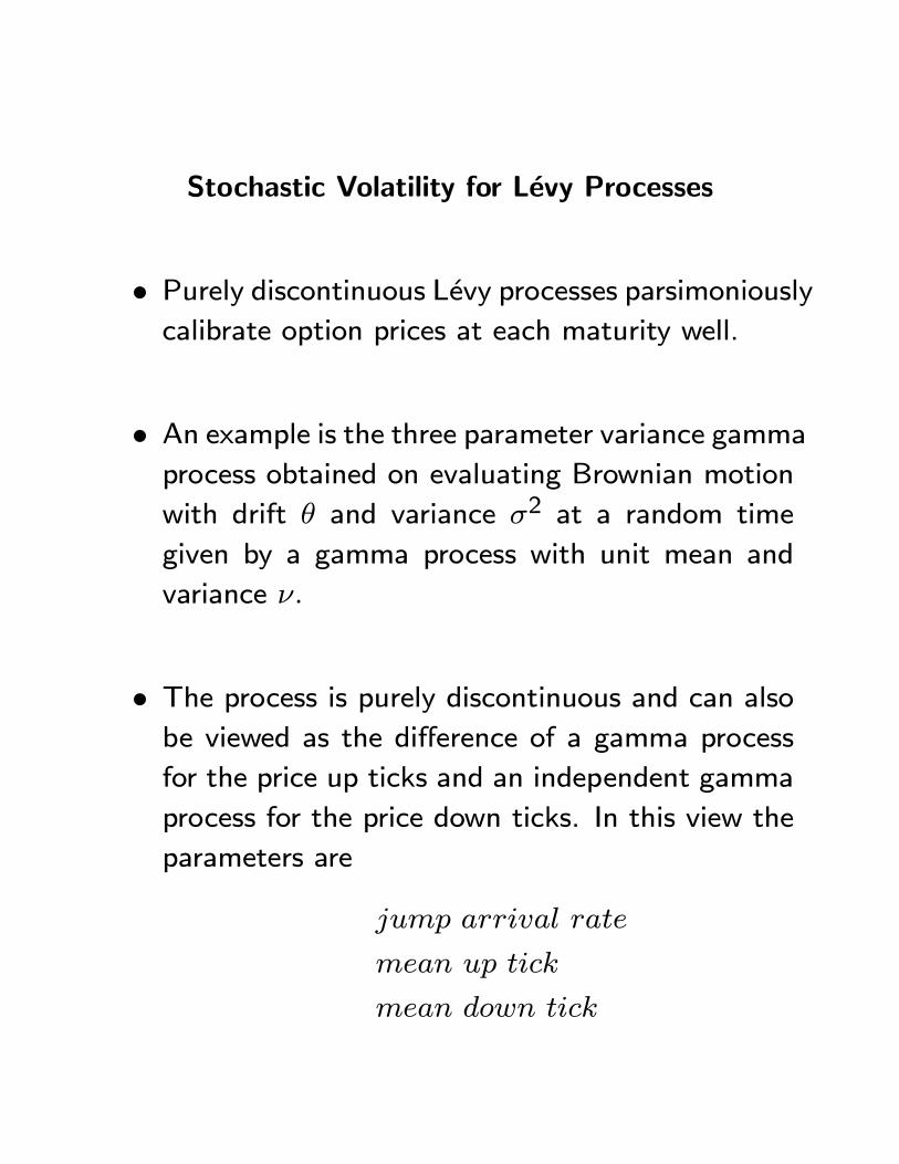
Stochastic Volatility for Levy Processes

• Purely discontinuous Levy processes parsimoniouslycalibrate option prices at each maturity well.

• An example is the three parameter variance gammaprocess obtained on evaluating Brownian motion

with drift θ and variance σ2 at a random time

given by a gamma process with unit mean and

variance ν.

• The process is purely discontinuous and can alsobe viewed as the difference of a gamma process

for the price up ticks and an independent gamma

process for the price down ticks. In this view the

parameters are

jump arrival rate

mean up tick

mean down tick

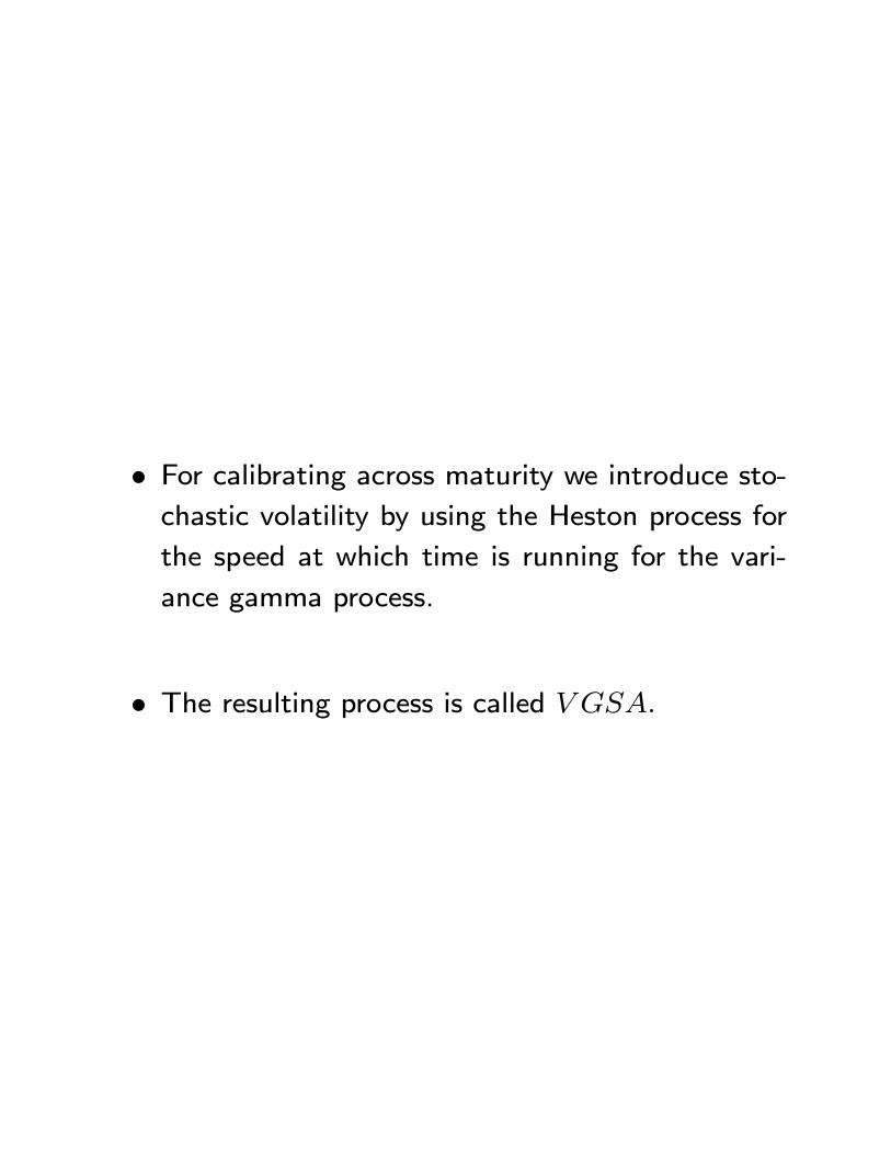
• For calibrating across maturity we introduce sto-chastic volatility by using the Heston process for

the speed at which time is running for the vari-

ance gamma process.

• The resulting process is called V GSA.

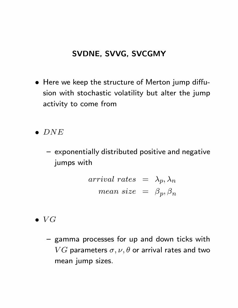
SVDNE, SVVG, SVCGMY

• Here we keep the structure of Merton jump diffu-sion with stochastic volatility but alter the jump

activity to come from

• DNE

— exponentially distributed positive and negative

jumps with

arrival rates = λp, λn

mean size = βp, βn

• V G

— gamma processes for up and down ticks with

V G parameters σ, ν, θ or arrival rates and two

mean jump sizes.

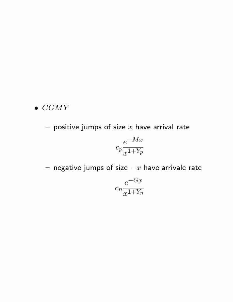
• CGMY

— positive jumps of size x have arrival rate

cpe−Mx

x1+Yp

— negative jumps of size −x have arrivale rate

cne−Gx

x1+Yn

Stochastic Jump Arrival Rates

• In all the above models, the arrival rate of jumpsis insensitive to the stochastic volatility. It isonly the continuous component or the infinites-imal jumps that respond to an increase in volatil-ity.

• In the stochastic arrival rate class of models welet the jump arrival rate have a linear response tothe stochastic volatility as well.

• We add this response to the SV DNE,SV V G, SV CGMYmodels and hence add two parameters for the re-sponse of the positive and negative jump arrivalrates to volatility to get the models SV ADNE,SV AV G, SV ACGMY. These new parametersare

sensitivity of positive arrival rate = sp

sensitivity of negative arrival rate = sn

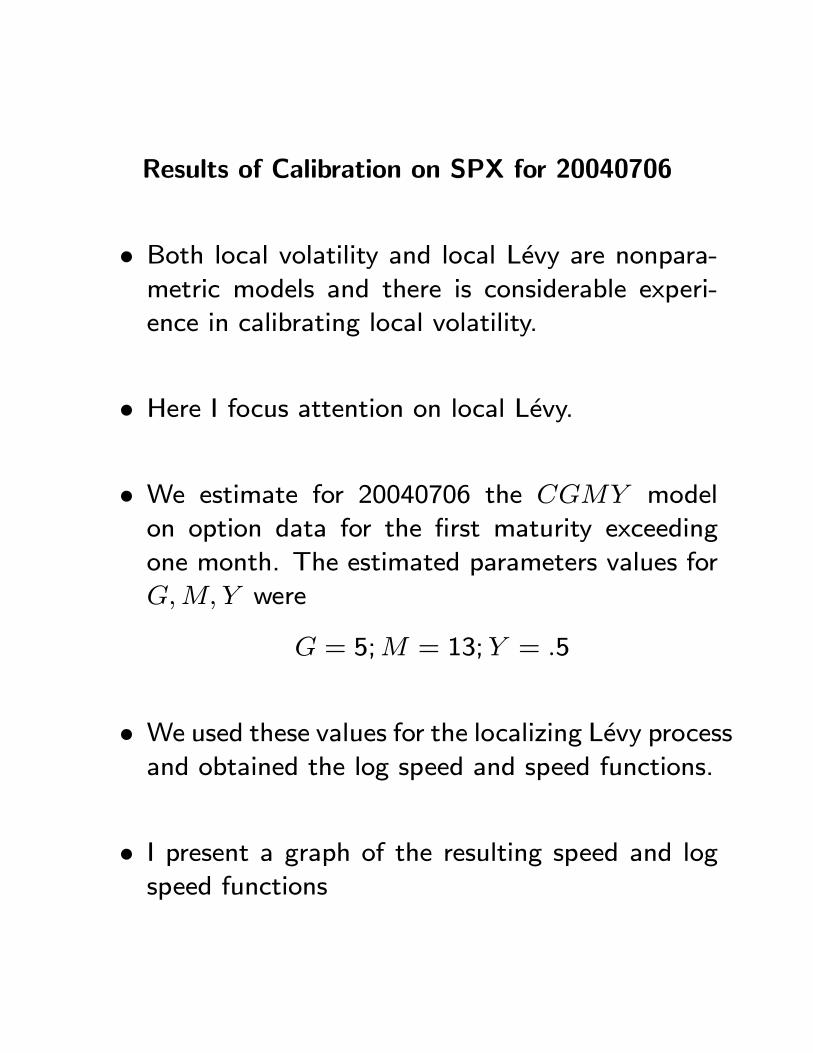
Results of Calibration on SPX for 20040706

• Both local volatility and local Levy are nonpara-metric models and there is considerable experi-ence in calibrating local volatility.

• Here I focus attention on local Levy.

• We estimate for 20040706 the CGMY modelon option data for the first maturity exceeding

one month. The estimated parameters values forG,M,Y were

G = 5;M = 13;Y = .5

• We used these values for the localizing Levy processand obtained the log speed and speed functions.

• I present a graph of the resulting speed and logspeed functions

−0.4

−0.2

0

0.2

0.4 0

0.2

0.4

0.6

0.8

1

0

5

10

15

20

25

30

35

time

logspeedmspx20041214

logreturn

5

10

15

20

25

30

Figure 2:

Remarks on Levy Speed Function

• The Speed lifts sharply at the short maturity downside as opposed to the up side.

• At the back end the Speed movement is relatively

0.70.8

0.91

1.11.2

1.31.4 0

0.2

0.4

0.6

0.8

1

0

5

10

15

20

time

speedmspx20041214

spot

Figure 3:

damped.

• This structure is comparable to what one is ac-customed to seeing for local volatility, except now

one is only purchasing part of the smile from the

spot depenence of speed or volatility.

• A considerable part has been hard wired by the

choice of an asymmetric localizing Levy process

with G = 5,M = 13 and 2% down moves coming

with a 16% greater frequency than 2% up moves.

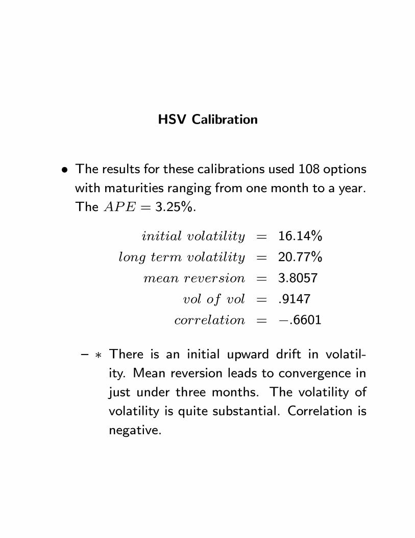
HSV Calibration

• The results for these calibrations used 108 optionswith maturities ranging from one month to a year.

The APE = 3.25%.

initial volatility = 16.14%

long term volatility = 20.77%

mean reversion = 3.8057

vol of vol = .9147

correlation = −.6601

— ∗ There is an initial upward drift in volatil-ity. Mean reversion leads to convergence in

just under three months. The volatility of

volatility is quite substantial. Correlation is

negative.

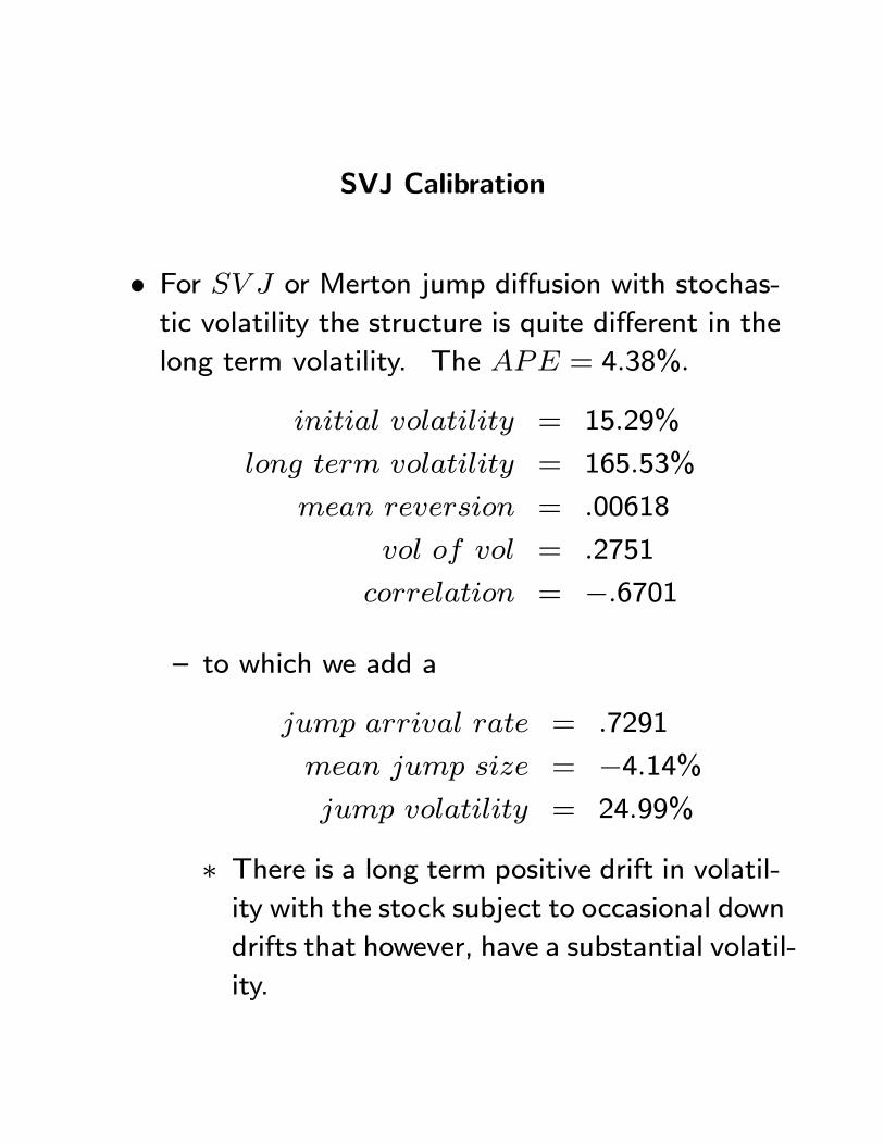
SVJ Calibration

• For SV J or Merton jump diffusion with stochas-

tic volatility the structure is quite different in the

long term volatility. The APE = 4.38%.



mean reversion = .00618

vol of vol = .2751


— to which we add a

jump arrival rate = .7291

mean jump size = −4.14%jump volatility = 24.99%

∗ There is a long term positive drift in volatil-

ity with the stock subject to occasional down

drifts that however, have a substantial volatil-

ity.

VGSA Calibration

• The APE = 2.67% .Stochastic volatility struc-

ture Parameter estimates are (C = 116.8068, G =

86.84,M = 114.536, κ = 5.5686, η = 65.7855, λ =

42.7730) we quote in volatility terms as




vol of vol = .3662

— and the jump structure is

M = 114.536

G = 86.84

∗ The calibration is characteristically very good.Mean reversion leads to convergence in a

few months. We have a slight down drift

in volatility to begin with. The jump moves

are on the small side with a slight skew to-

wards the negative moves.

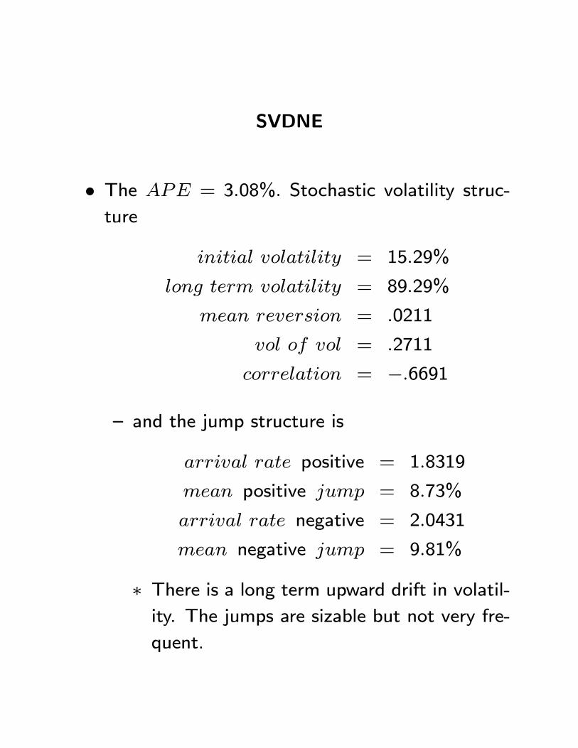
SVDNE

• The APE = 3.08%. Stochastic volatility struc-

ture




vol of vol = .2711



arrival rate positive = 1.8319

mean positive jump = 8.73%

arrival rate negative = 2.0431

mean negative jump = 9.81%

∗ There is a long term upward drift in volatil-

ity. The jumps are sizable but not very fre-

quent.

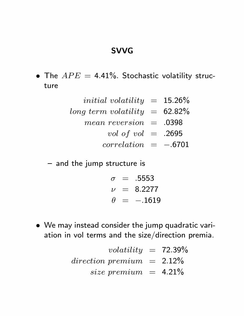
SVVG

• The APE = 4.41%. Stochastic volatility struc-ture




vol of vol = .2695



σ = .5553

ν = 8.2277

θ = −.1619

• We may instead consider the jump quadratic vari-ation in vol terms and the size/direction premia.

volatility = 72.39%

direction premium = 2.12%

size premium = 4.21%

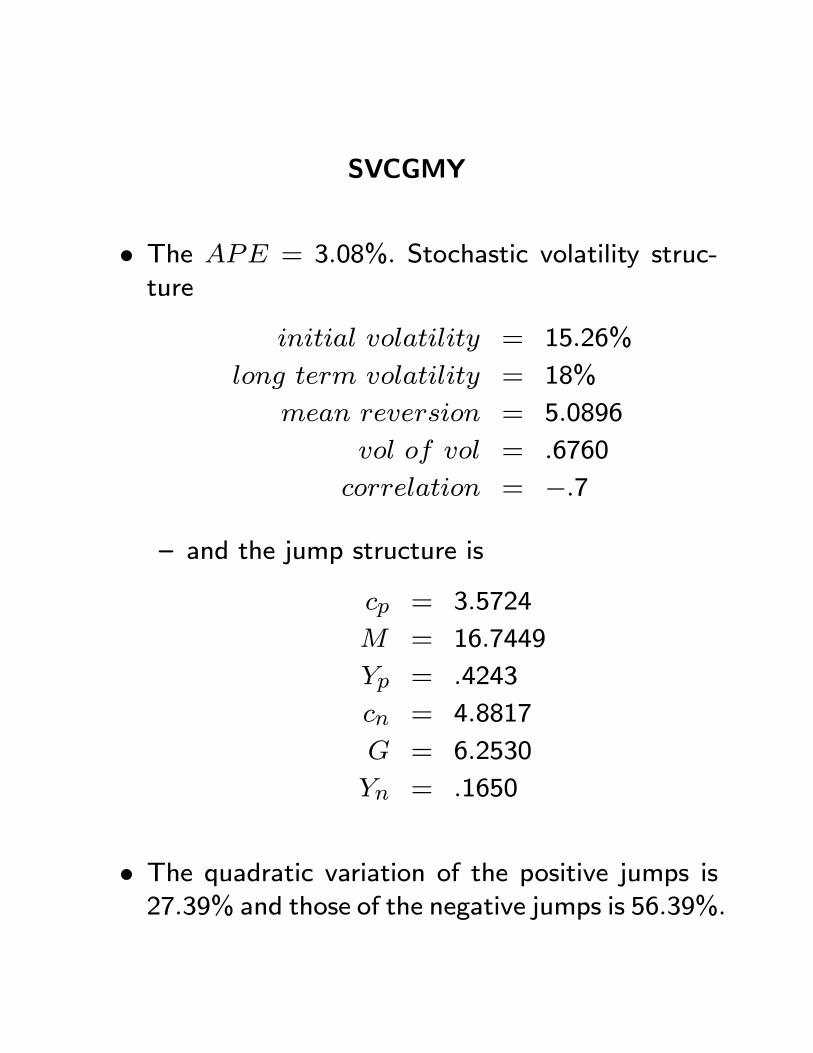
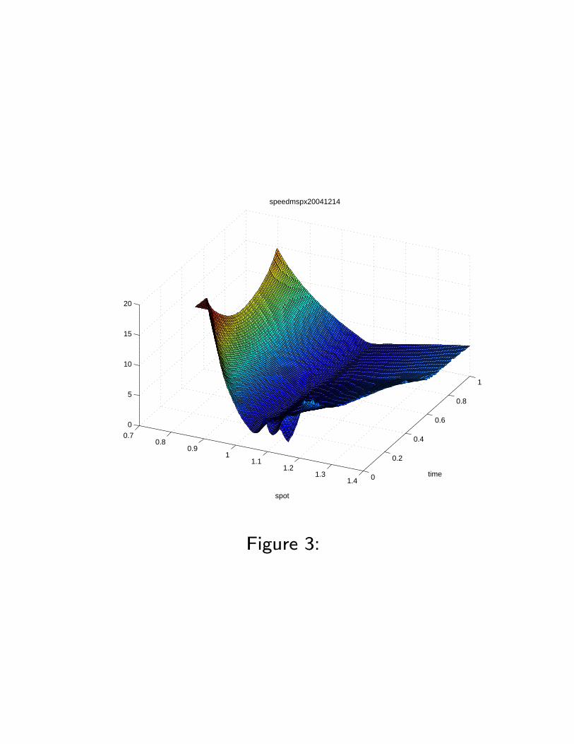
SVCGMY

• The APE = 3.08%. Stochastic volatility struc-ture


long term volatility = 18%


vol of vol = .6760

correlation = −.7


cp = 3.5724

M = 16.7449

Yp = .4243

cn = 4.8817

G = 6.2530

Yn = .1650

• The quadratic variation of the positive jumps is27.39% and those of the negative jumps is 56.39%.

SVADNE


ture




vol of vol = .5203



positive arrival rate = 4.3001

positive sensitivity = 3.4077

mean size = 10.05%

negative arrival rate = 3.1290

negative sensitivity = .000666

mean size = 20.31%

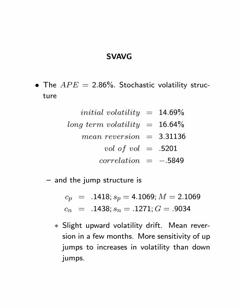
SVAVG


ture




vol of vol = .5201



cp = .1418; sp = 4.1069;M = 2.1069

cn = .1438; sn = .1271;G = .9034

∗ Slight upward volatility drift. Mean rever-sion in a few months. More sensitivity of up

jumps to increases in volatility than down

jumps.

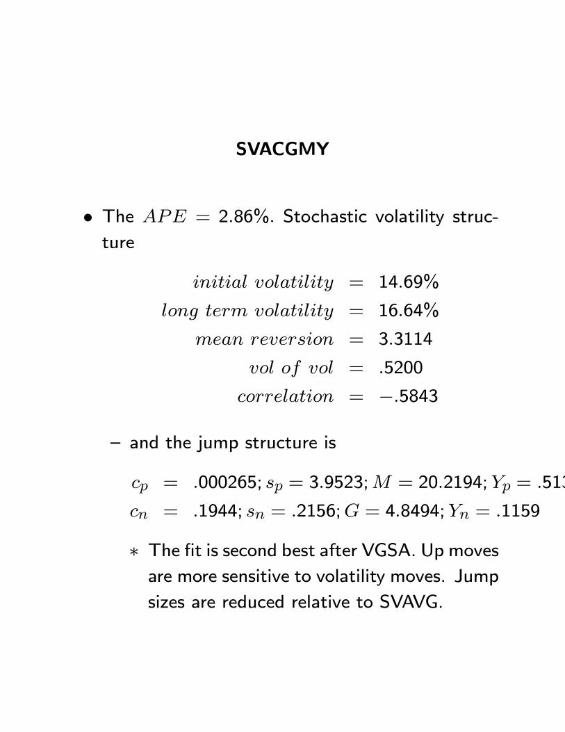
SVACGMY


ture




vol of vol = .5200



cp = .000265; sp = 3.9523;M = 20.2194;Yp = .513

cn = .1944; sn = .2156;G = 4.8494;Yn = .1159

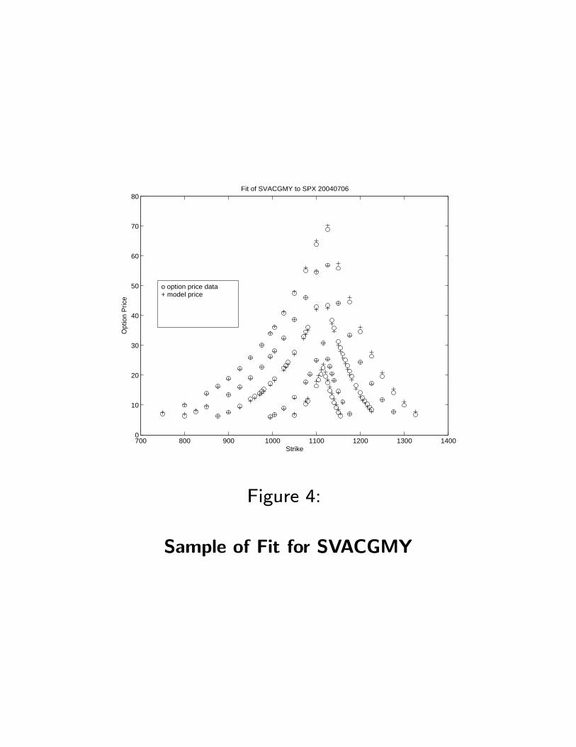
∗ The fit is second best after VGSA. Up movesare more sensitive to volatility moves. Jump

sizes are reduced relative to SVAVG.

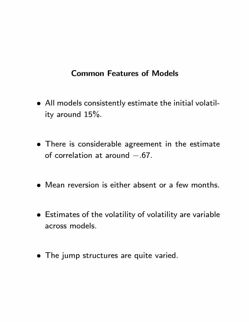
Common Features of Models

• All models consistently estimate the initial volatil-ity around 15%.

• There is considerable agreement in the estimateof correlation at around −.67.

• Mean reversion is either absent or a few months.

• Estimates of the volatility of volatility are variableacross models.

• The jump structures are quite varied.

700 800 900 1000 1100 1200 1300 14000

10

20

30

40

50

60

70

80Fit of SVACGMY to SPX 20040706

Strike

Opt

ion

Pric

e

o option price data+ model price

Figure 4:

Sample of Fit for SVACGMY

The Products Priced by the Models

• We priced six products for all 11 models. Theseare

— Locally Floored and Globally Capped 4 year

monthly monitored Arithmetic Cliquet with three

local floors at −10,−7.5,−5 and global capsat 10, 20, 30, 40, and 50.

— Locally capped and Globally Floored 4 year

monthly monitored Arithmetic Cliquet with three

local caps at 5, 7.5, 10 and global floors at

−50,−40,−30,−20 and −10.

— 4 year monthly monitored Arithmetic Swing

cliquet with strikes 5, 6, 7, 8, 9 and 10 and three

caps at 80, 90 and 100.

— 4 year monthly monitored Arithmetic Reverse

Swing Cliquet with local caps at 5, 10, 15, 20, 25.

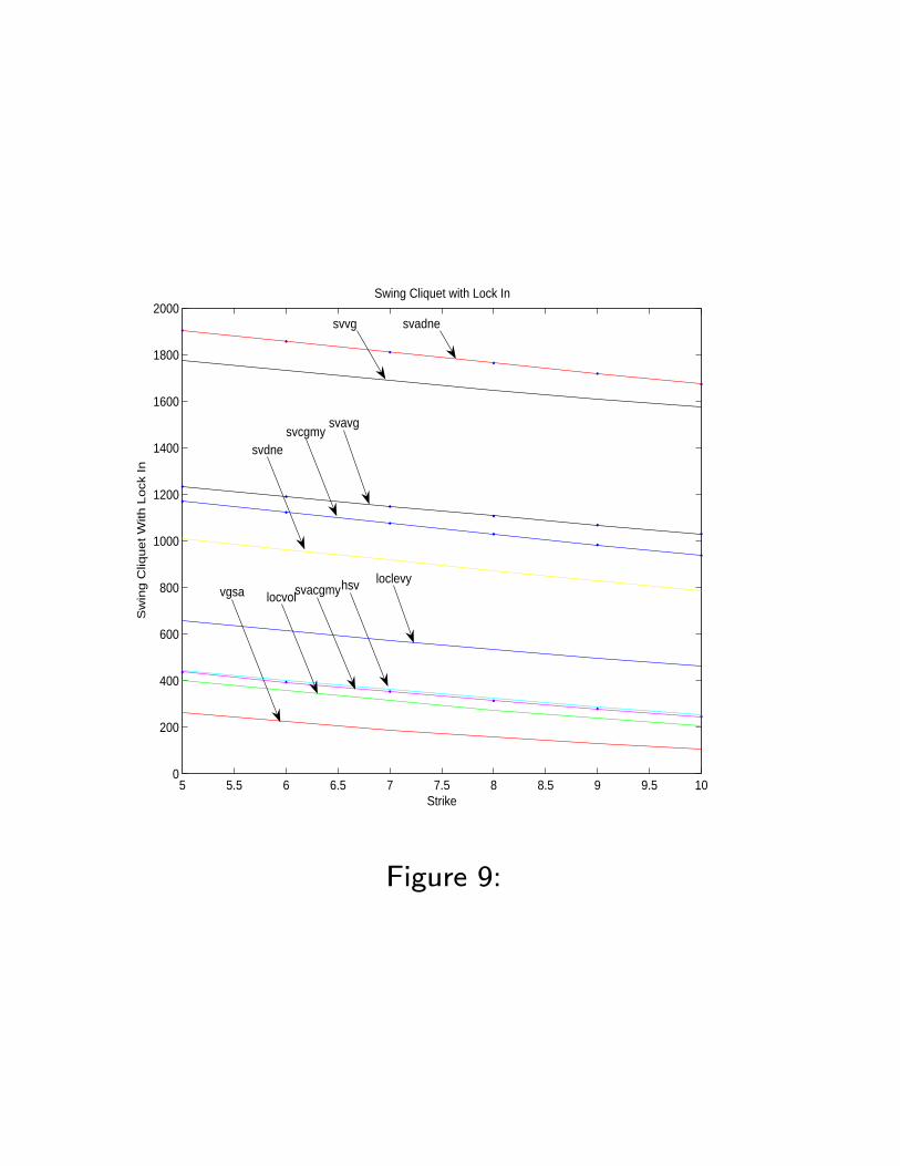
— 4 year monthly monitored Arithmetic Swing

Cliquet with Lock In and no caps, for strikes

5, 6, 7, 8, 9 and 10.

— TARN with down barriers at 50 to 70 in steps

of 2, cancellation at levels 110, 120, 130, 140

at 6%, 12%, 18%, 24% and long an at-the-money

call in the absence of cancellation or the down

event.

Model Pricing

• For the Locally-Floored and Globally capped cli-quets we have for each model 15 prices for three

floors five caps.

• The prices rise as we raise the caps five times andthen fall for the raised floor but lowest cap.

• We graph these 15 prices for all models.

Locally Floored Globally Capped Cliquet Model

Rankings

• For this product the average contract prices inrank order are

SVADNE 27.22SVCGMY 26.33LL 24.46SVJ 22.91SVDNE 18.14HSV 17.03SVAVG 16.60LV 16.26SVVG 14.94SVACGMY 11.99VGSA 8.56

0 5 10 15−10

0

10

20

30

40

50Locally Floored and Globally Capped Cliquet

local levy

local vol

vgsa

hsv

svj

svdne

svvg

svcgmy

svadne

svavg

svaccgmyy

Figure 5:

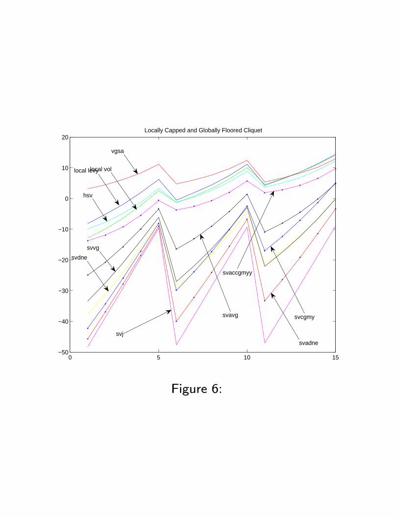
Locally Capped and Globally Floored Cliquet

• Here we three local caps and five global floors.

• The value rises as we raise the floors and falls aswe get to the next lowest cap with a higher floor.

• We observe that some models like SV J are really

exposed to the absence of the local floor and have

values stretching down to meet the global floor.

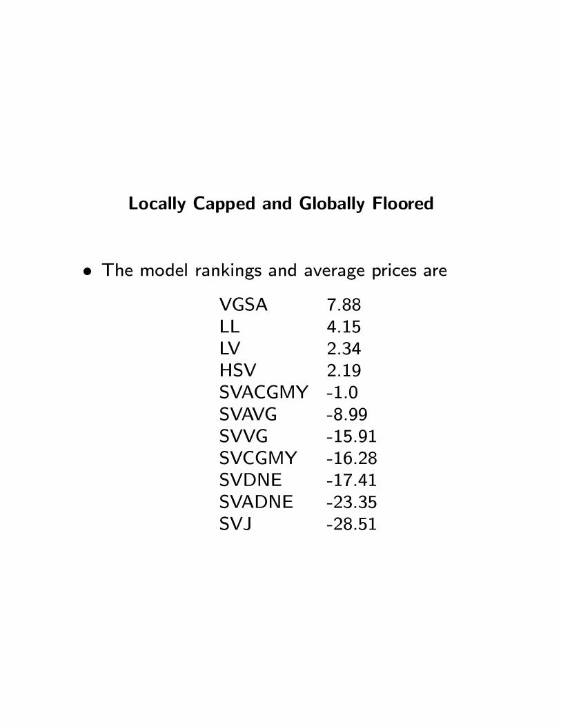
Locally Capped and Globally Floored

• The model rankings and average prices areVGSA 7.88LL 4.15LV 2.34HSV 2.19SVACGMY -1.0SVAVG -8.99SVVG -15.91SVCGMY -16.28SVDNE -17.41SVADNE -23.35SVJ -28.51

0 5 10 15−50

−40

−30

−20

−10

0

10

20Locally Capped and Globally Floored Cliquet

local levylocal vol

vgsa

hsv

svj

svdne

svvg

svcgmy

svadne

svavg

svaccgmyy

Figure 6:

Capped Swing Cliquet

• We have six strikes and three caps.

The value drops as we raise the strikes and rises as we

raise the cap.

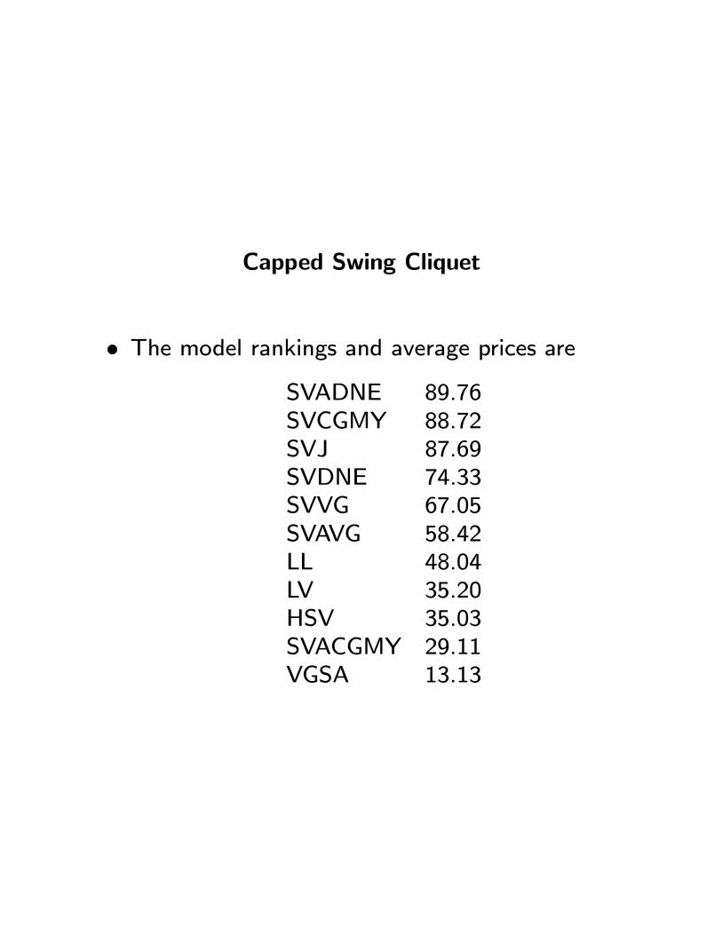
Capped Swing Cliquet

• The model rankings and average prices areSVADNE 89.76SVCGMY 88.72SVJ 87.69SVDNE 74.33SVVG 67.05SVAVG 58.42LL 48.04LV 35.20HSV 35.03SVACGMY 29.11VGSA 13.13

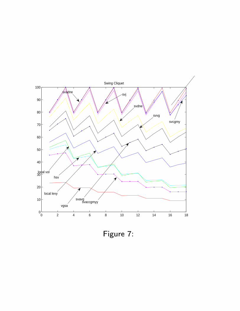
0 2 4 6 8 10 12 14 16 180

10

20

30

40

50

60

70

80

90

100Swing Cliquet

local levy

local vol

vgsa

hsv

svj

svdne

svvg

svcgmy

svadne

svavgsvaccgmyy

Figure 7:

Capped Reverse Swing Cliquet

• We have five caps for the reverse swing cliquet.

• The value rises as we raise the cap.

Reverse Swing Cliquet

• The model rankings and average prices areVGSA 596.31SVACGMY 559.27HSV 551.03SVAVG 544.22LL 541.07SVVG 519.39LV 513.61SVDNE 481.55SVADNE 428.47SVCGMY 393.60SVJ 137.21

5 10 15 20 250

200

400

600

800

1000

1200Reverse Swing Cliquet

Cap

Reve

rse S

win

g C

liquet

local levy

local vol

vgsa

hsv

svj

svdne

svvg

svcgmy

svadne

svavg

svacgmy

Figure 8:

Uncapped Swing Cliquet with Lock In

• We have six strikes with value falling as we raisethe strike.

• The Lock In gives substantial value to the con-tract.

• The Lock In also exaggerates the model differ-ences.

• We drop SV J as the value is too exagerated.

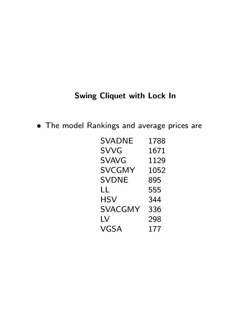
Swing Cliquet with Lock In

• The model Rankings and average prices areSVADNE 1788SVVG 1671SVAVG 1129SVCGMY 1052SVDNE 895LL 555HSV 344SVACGMY 336LV 298VGSA 177

5 5.5 6 6.5 7 7.5 8 8.5 9 9.5 100

200

400

600

800

1000

1200

1400

1600

1800

2000Swing Cliquet with Lock In

Strike

Sw

ing C

liquet W

ith L

ock

In

vgsa locvolsvacgmyhsv loclevy

svdnesvcgmy

svavg

svvg svadne

Figure 9:

Trigger Autocancellable Redeemable Note

• We have 11 down barrier strikes with value risingas we raise the strike and limit the loss experi-

enced.

• Again we drop SV J.

Trigger Autocancellable Redeemable Note

• The model prices and rankings areLL 70.62SVCGMY 69.49LV 67.61SVADNE 67.16SVDNE 64.96SVAVG 63.35HSV 59.96VGSA 58.16SVVG 57.24SVACGMY 53.27

50 52 54 56 58 60 62 64 66 68 7045

50

55

60

65

70

75Trigger Autocancellable Redeemable Note

Strike

TA

RN

PR

ICE

local Levy svcgmylocal vol

svadne

svdne svavg hsv

vgsa

svvgsvacgmy

Figure 10:

Model Rank Correlations

• The rankings of the 10 models, excluding SV J,

across the six products are

LFGC LCGF S RS SWLIN TARNLL 3 2 6 5 6 1LV 7 3 7 7 9 3VGSA 10 1 10 1 10 8HSV 5 4 8 3 7 7SVDNE 4 9 3 8 5 5SVDVG 8 7 4 6 2 6SVCGMY 2 8 2 10 4 2SVADNE 1 10 1 9 1 4SVAVG 6 6 5 4 3 9SVACGMY 9 5 9 2 8 10

• The model rank correlations between the productsare

LFGC LCGF S RS SWLIN TARNLFGC 1 -.56 .78 -.76 .59 .68LCGF -.56 1 -.87 .72 -.81 -.10S .78 -.87 1 -.90 .87 .52RS -.76 .72 -.90 1 -.60 -.72SWLIN .59 -.81 .87 -.60 1 .19TARN .68 -.10 .52 -.72 .19 1

• We expect that quite naturally when hedging toacceptability, one would quite often be using dif-

ferent models for different products.

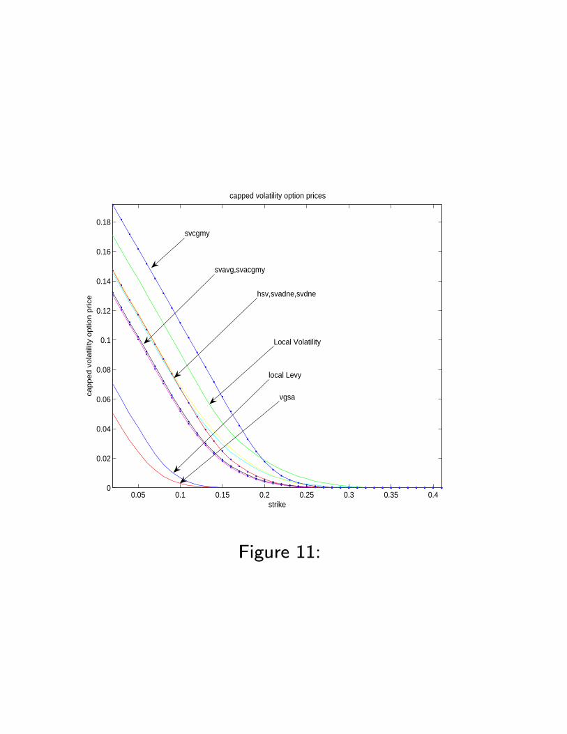
Volatility Options

• We now consider the one year capped volatility

options that pays at the end of the year

Max

252 TX

t=1

Min

Ãln(St/St−1)2

T,cap2

252

!1/2 − k, 0

• We present a graph of the valuations from 9 cal-

ibrated models of this contract.

Risks in Equity Structured Products

• Each model when simulated for the evaluation ofthe price may also be used to detect the nature

of the risk in the product, at least as this is seen

from the perspective of the model.

• For each forward date one may use the simulatedcash flows to construct the forward spot slide us-

ing a kernel estimator for the value function.

0.05 0.1 0.15 0.2 0.25 0.3 0.35 0.40

0.02

0.04

0.06

0.08

0.1

0.12

0.14

0.16

0.18

capped volatility option prices

strike

cap

pe

d v

ola

tility

op

tion

price

vgsa

local Levy

Local Volatility

hsv,svadne,svdne

svavg,svacgmy

svcgmy

Figure 11:

• Say we are interested in the value of the struc-tured product at forward time n when the spot is

at p. Let cs be the simulated cash flow on path s

and let ps be the price of the underlying on path

s at time n. The kernel estimator for the value at

n when the spot is at p, V (p, n) is

V (p, n) =Xs

ws(p, ps)cs

where the weights ws(p, ps) are a normalization

of the sequence

exp

Ã−µp− ps

2h

¶2!

for a prespecified band width h.

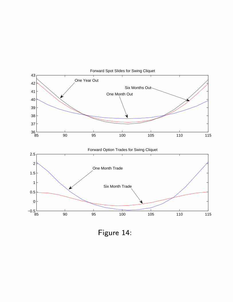
Forward Spot Slides and Option Trades

• We illustrate here for the locally floored, globallycapped (LFGC), locally capped globally floored

(LCGF ) and swing (S) cliquet under the model

SV ACGMY.

• The top graph is the spot slide for one month out,six months out and one year out.

• The bottom graph plots the difference in value

functions and gives the option trade needed to

hedge the change in the value function.

Implicit Hedge Costs

• We see that for LFGC we have the forward risk of

acquiring some out of the money puts and selling

some out of the money calls.

— An increase in the skew will make this trade

more expensive and hence the strong skew

delta and gamma of this position.

• In contrast, the swing cliquet has us buying outof the money calls and puts.

— Hence the exposure to volgamma in this case.

85 90 95 100 105 110 11510

11

12

13

14

15

16Forward Spot Slides for LFGC

85 90 95 100 105 110 115−0.8

−0.6

−0.4

−0.2

0

0.2

0.4

0.6Forward Option Trades for LFGC

One Month Out

Six Months Out

One Year Out

One Month Trade

Six Month Trade

Figure 12:

85 90 95 100 105 110 115−12

−10

−8

−6

−4

−2Forward Spot Slides for LCGF

85 90 95 100 105 110 115−1.5

−1

−0.5

0

0.5

1Forward Option Trades for LCGF

One Month Out

Six Months Out

One Year Out

One Month TradeSix Months Trade

Figure 13:

85 90 95 100 105 110 11536

37

38

39

40

41

42

43Forward Spot Slides for Swing Cliquet

85 90 95 100 105 110 115−0.5

0

0.5

1

1.5

2

2.5Forward Option Trades for Swing Cliquet

One Month Out

Six Months Out

One Year Out

One Month Trade

Six Month Trade

Figure 14:

Conclusion

• Equity Structured Products are a desirable way ofrisk positioning for the investing public.

• Model contingent hedging and valuation is feasi-ble for the supplier.

• It is a consequence of hedging to acceptabilitythat different models be used to support the val-

uation and hedging of different products.

— In fact even for the same product, different

models are the support for the bid and the

ask price.

• Differences in model prices are therefore not anelement of model risk.

• Model risk is about the spread of models to beused in the valuation and hedging activity and

it is this spread of models that constitutes the

definition of acceptability, that is the fundamental

core concept being modeled.

Documents

Best Practice Modeling for Equity Structured Products · OUTLINE • Description of Models and their properties. • Results of Market Calibration. • Model Prices for Equity Structured