Embed Size (px)
Citation preview
Journal of Functional Analysis 258 (2010) 1628–1655
www.elsevier.com/locate/jfa
Besov spaces with variable smoothness and integrability
Alexandre Almeida a,1, Peter Hästö b,∗,2
a Department of Mathematics, University of Aveiro, 3810-322 Aveiro, Portugalb Department of Mathematical Sciences, PO Box 3000, FI-90014 University of Oulu, Finland
Received 24 June 2009; accepted 16 September 2009
Available online 22 September 2009
Communicated by N. Kalton
Abstract
In this article we introduce Besov spaces with variable smoothness and integrability indices. We proveindependence of the choice of basis functions, as well as several other basic properties. We also giveSobolev-type embeddings, and show that our scale contains variable order Hölder–Zygmund spaces as spe-cial cases. We provide an alternative characterization of the Besov space using approximations by analyticfunctions.© 2009 Elsevier Inc. All rights reserved.
Keywords: Non-standard growth; Variable exponent; Besov space; Iterated Lebesgue spaces; Hölder–Zygmund space;Sobolev embedding; Approximation
1. Introduction
Spaces of variable integrability, also known as variable exponent function spaces, can betraced back to 1931 and W. Orlicz [29], but the modern development started with the paper [24]of Kovácik and Rákosník in 1991. Corresponding PDE with non-standard growth have beenstudied since the same time. For an overview we refer to the surveys [14,21,30,36] and themonograph [13]. Apart from interesting theoretical considerations, the motivation to study such
* Corresponding author.E-mail addresses: [email protected] (A. Almeida), [email protected] (P. Hästö).URL: http://cc.oulu.fi/~phasto/ (P. Hästö).
1 Supported in part by INTAS and the Research Unit Matemática e Aplicações of University of Aveiro.2 Supported in part by the Academy of Finland, the Emil Aaltonen Foundation and INTAS.
0022-1236/$ – see front matter © 2009 Elsevier Inc. All rights reserved.doi:10.1016/j.jfa.2009.09.012

A. Almeida, P. Hästö / Journal of Functional Analysis 258 (2010) 1628–1655 1629
function spaces comes from applications to fluid dynamics [1,2,34], image processing [11], PDEand the calculus of variation [3,16,18,20,28,35,47].
In a recent effort to complete the picture of the variable exponent Lebesgue and Sobolevspaces, Almeida and Samko [4] and Gurka, Harjulehto and Nekvinda [19] introduced variableexponent Bessel potential spaces Lα,p(·) with constant α ∈ R. As in the classical case, this spacecoincides with the Lebesgue/Sobolev space for integer α. There was taken a step further by Xu[44–46], who considered Besov Bα
p(·),q and Triebel–Lizorkin Fαp(·),q spaces with variable p, but
fixed q and α.Along a different line of inquiry, Leopold [25–27] studied pseudo-differential operators with
symbols of the type 〈ξm(x)〉, and defined related function spaces of Besov-type with variablesmoothness, B
m(·)p,p . In fact, Beauzamy [7] had studied similar Ψ DEs already in the beginning of
the 70s. Function spaces of variable smoothness have recently been studied by Besov [8–10]: hegeneralized Leopold’s work by considering both Triebel–Lizorkin spaces F
α(·)p,q and Besov spaces
Bα(·)p,q in R
n. By way of application, Schneider and Schwab [39] used Bm(·)2,2 (R) in the analysis of
certain Black–Scholes equations. For further considerations of Ψ DEs, we refer to Hoh [22] andreferences therein.
Integrating the above mentioned spaces into a single larger scale promises similar gains andsimplifications as were seen in the constant exponent case in the 60s and 70s with the advent ofthe full Besov and Triebel–Lizorkin scales. Most of the advantages of unification do not occurwith only one index variable: for instance, traces or Sobolev embeddings cannot be covered inthis case, since they involve an interaction between integrability and smoothness. To tackle this,Diening, Hästö and Roudenko [15] introduced Triebel–Lizorkin spaces with all three indicesvariable, F
α(·)p(·),q(·) and showed that they behaved nicely with respect to trace. Subsequently, Vy-
bíral [43] proved Sobolev (Jawerth) type embeddings in these spaces; they were also studied byKempka [23]. These studies were all restricted to bounded exponents p and q .
Vybíral [43] and Kempka [23] also considered Besov spaces Bα(·)p(·),q—note that only the case
of constant q was included. This is quite natural, since the norm in the Besov space is usuallydefined via the iterated space �q(Lp) so that the space integration in Lp is done first, followedby the sum over frequency scales in �q . Therefore, it is not obvious how q could depend on x,which has already been integrated out. It is the purpose of the present paper to propose a methodmaking this dependence possible and thus completing the unification process in the variableintegrability-smoothness case by introducing the Besov space B
α(·)p(·),q(·) with all three indices
variable.Our space includes the previously mentioned spaces of Besov-type, as well as the Hölder–
Zygmund space Cα(·). As in the constant exponent case, it is possible to consider unboundedexponents p and q in the Besov space case, while for the Triebel–Lizorkin space one needs p
to be bounded. Another advantage of the Besov space for constant exponent is its simplicitycompared to the Triebel–Lizorkin space; for instance, the latter requires vector-valued maximaland multiplier theorems, whereas the simple scalar case suffices in the Besov case. Unfortunately,this is not true for the generalization with variable q (this is to be expected, see Remark 4.2 fora discussion). We will nevertheless see that working in the Besov space is relatively simpleonce some basic tools have been established for dealing in the “iterated” space �q(·)(Lp(·)) inSections 3 and 4.
We then define the Besov space Bα(·)p(·),q(·) in Section 5 and give several basic properties estab-
lishing the soundness of our definition. In Section 6 we prove elementary embeddings betweenBesov and Triebel–Lizorkin spaces, as well as Sobolev embeddings in the Besov scale. In Sec-

1630 A. Almeida, P. Hästö / Journal of Functional Analysis 258 (2010) 1628–1655
tion 7 we show that our scale includes the variable order Hölder–Zygmund space as a specialcase: B
α(·)∞,∞ = Cα(·) for 0 < α < 1. In Section 8 we give an alternative characterization of theBesov space by means of approximations by analytic functions.
Before starting our main presentation with some conventions and results on semimodular andvariable exponent spaces, we point out one possible interesting avenue for future research whichmight be opened by this work: real interpolation. So far, complex interpolation has been consid-ered in the variable exponent context in [13,14]. Real interpolation, however, is more difficult inthis setting. Using standard notation, we have, for constant exponents,(
Lp0 ,Lp1)θ,q
= Lpθ ,q ,
where 1/pθ := θ/p0 + (1 − θ)/p1 and Lpθ ,q is the Lorenz space. To obtain interpolation ofLebesgue spaces one simply chooses q = pθ . Although details have not been presented anywhereas best we know, it seems that there are no major difficulties in letting p0 and p1 be variable here,i.e. (
Lp0(·),Lp1(·))θ,q
= Lpθ (·),q ,
where pθ is defined point-wise by the same formula as before. However, this time we do notobtain an interpolation result in Lebesgue spaces, since we cannot set the constant q equal to thefunction pθ . In fact, the role of q in the real interpolation method is quite similar to the role of q
in the Besov space Bαp,q . Therefore, we hope that the approach introduced in this paper for Besov
spaces with variable q will also allow us to generalize real interpolation properly to the variableexponent context. Another interesting challenge is to extend extrapolation [12] to the setting ofBesov spaces.
2. Preliminaries
In this section we introduce some conventions and notation, and state some basic results. Forthe latter we refer to [13, Chapters 1–3].
We use c as a generic positive constant, i.e. a constant whose value may change from ap-pearance to appearance. The expression f ≈ g means that 1
cg � f � cg for some suitably
independent constant c. By χA we denote the characteristic function of A ⊂ Rn. By suppf
we denote the support of the function f , i.e. the closure of its zero set. The notation X ↪→ Y
denotes continuous embeddings from X to Y .
2.1. Modular spaces
The spaces studied in this paper fit into the framework of so-called semimodular spaces. Foran exposition of these concepts we refer to the monographs [13,31]. We recall the followingdefinition:
Definition 2.1. Let X be a vector space over R or C. A function :X → [0,∞] is called a semi-modular on X if the following properties hold:
(1) (0) = 0.(2) (λf ) = (f ) for all f ∈ X and |λ| = 1.

A. Almeida, P. Hästö / Journal of Functional Analysis 258 (2010) 1628–1655 1631
(3) (λf ) = 0 for all λ > 0 implies f = 0.(4) λ → (λf ) is left-continuous on [0,∞) for every f ∈ X.
A semimodular is called a modular if
(5) (f ) = 0 implies f = 0.
A semimodular is called continuous if
(6) for every f ∈ X the mapping λ → (λf ) is continuous on [0,∞).
A semimodular can be additionally qualified by the term (quasi)convex. This means, asusual, that
(θf + (1 − θ)g
)� A
[θ(f ) + (1 − θ)(g)
],
for all f,g ∈ X; here A = 1 in the convex case, and A ∈ [1,∞) in the quasiconvex case.Once we have a semimodular in place, we obtain a normed space in a standard way:
Definition 2.2. If is a (semi)modular on X, then
X := {x ∈ X: ∃λ > 0, (λx) < ∞}
is called a (semi)modular space.
Theorem 2.3. Let be a (quasi)convex semimodular on X. Then X is a (quasi)normed spacewith the Luxemburg (quasi)norm given by
‖x‖ := inf
{λ > 0:
(1
λx
)� 1
}.
For simplicity we will refer to semimodulars as modulars except when special clarity isneeded; similarly, we later drop the word “quasi”.
One key method for dealing with the somewhat complicated definition of a norm is the fol-lowing relationship which follows from the definition and left-continuity: (f ) � 1 if and onlyif ‖f ‖ � 1.
2.2. Spaces of variable integrability
The variable exponents that we consider are always measurable functions on Rn with range
(c,∞] for some c > 0. We denote the set of such functions by P0. The subset of variable expo-nents with range [1,∞] is denoted by P . For A ⊂ R
n and p ∈ P0 we denote p+A = ess supA p(x)
and p−A = ess infA p(x); we abbreviate p+ = p+
Rn and p− = p−Rn .
The function ϕp is defined as follows:
ϕp(t) =⎧⎨⎩
tp if p ∈ (0,∞),
0 if p = ∞ and t � 1,
∞ if p = ∞ and t > 1.
1632 A. Almeida, P. Hästö / Journal of Functional Analysis 258 (2010) 1628–1655
The convention 1∞ = 0 is adopted in order that ϕp be left-continuous. In what follows wewrite tp instead of ϕp(t), with this convention implied. The variable exponent modular is de-fined by
p(·)(f ) :=∫Rn
ϕp(x)
(∣∣f (x)∣∣)dx.
The variable exponent Lebesgue space Lp(·) and its norm ‖f ‖p(·) are defined by the modularas explained in the previous subsection. The variable exponent Sobolev space Wk,p(·) is thesubspace of Lp(·) consisting of functions f whose distributional k-th order derivative exists andsatisfies |Dkf | ∈ Lp(·) with norm
‖f ‖Wk,p(·) = ‖f ‖p(·) + ∥∥Dkf∥∥
p(·).
We say that g : Rn → R is locally log-Hölder continuous, abbreviated g ∈ C
logloc , if there exists
clog > 0 such that
∣∣g(x) − g(y)∣∣ � clog
log(e + 1/|x − y|)
for all x, y ∈ Rn. We say that g is globally log-Hölder continuous, abbreviated g ∈ Clog, if it is
locally log-Hölder continuous and there exists g∞ ∈ R such that
∣∣g(x) − g∞∣∣ � clog
log(e + |x|)
for all x ∈ Rn. The notation P log is used for those variable exponents p ∈ P with 1
p∈ Clog.
The class P log0 is defined analogously. If p ∈ P log, then convolution with a radially decreasing
L1-function is bounded on Lp(·):
‖ϕ ∗ f ‖p(·) � c‖ϕ‖1‖f ‖p(·).
3. The mixed Lebesgue-sequence space
In this section we introduce a generalization of the iterated function space �q(Lp(·)) for thecase of variable q , which allows us to define Besov spaces with variable q in Section 5. We givea general but quite strange looking definition for the mixed Lebesgue-sequence space modular.This is not strictly an iterated function space—indeed, it cannot be, since then there would beno space variable left in the outer function space. To motivate our definition, we show that ithas several sensible properties (Examples 3.2 and 3.4) and that it concurs with the iterated spacewhen q is constant (Proposition 3.3). Then we show that our modular in fact is a semimodular inthe sense defined in the previous section and conclude that it defines a normed space.

A. Almeida, P. Hästö / Journal of Functional Analysis 258 (2010) 1628–1655 1633
Definition 3.1. Let p,q ∈ P0. The mixed Lebesgue-sequence space �q(·)(Lp(·)) is defined onsequences of Lp(·)-functions by the modular
�q(·)(Lp(·))((fν)ν
) :=∑ν
inf{λν > 0
∣∣ p(·)(fν/λ
1q(·)ν
)� 1
}.
Here we use the convention λ1/∞ = 1. The norm is defined from this as usual:
∥∥(fν)ν∥∥
�q(·)(Lp(·)) := inf
{μ > 0
∣∣∣ �q(·)(Lp(·))
(1
μ(fν)ν
)� 1
}.
If q+ < ∞, then
inf{λ > 0
∣∣ p(·)(f/λ
1q(·)
)� 1
} = ∥∥|f |q(·)∥∥p(·)q(·)
.
Since the right-hand side expression is much simpler, we use this notation to stand for the left-hand side even when q+ = ∞. For instance, we often use the notation
�q(·)(Lp(·))((fν)ν
) =∑ν
∥∥|fν |q(·)∥∥p(·)q(·)
for the modular.The norm in �q(·)(Lp(·)) is usually quite complicated to calculate. Here are some examples
where it is possible to simplify its expression.
Example 3.2. Suppose that p ≡ ∞. Then
�q(·)(L∞)
((fν)ν
) =∑ν
inf{λν > 0
∣∣ ∞(fν/λ
1q(·)ν
)� 1
}.
Now ∞(g) � 1 if and only if |g| � 1 almost everywhere. Thus |fν |/λ1
q(·)ν � 1 a.e., hence λν �
ess supx |fν(x)|q(x). It follows that
�q(·)(L∞)
((fν)ν
) =∑ν
ess supx
∣∣fν(x)∣∣q(x)
.
Note how the case q(x) = ∞ is included by the convention t∞ = ∞χ(1,∞)(t).
Another considerable simplification occurs when q is a constant. In this case �q(Lp(·)) isreally an iterated function space in the sense that we take the �q -norm of Lp(·)-norms as we nowshow. This also justifies the notation �q(·)(Lp(·)) even though this is not in general an iteratedspace.
Proposition 3.3. If q ∈ (0,∞] is constant, then
∥∥(fν)ν∥∥
�q (Lp(·)) = ∥∥‖fν‖p(·)∥∥
�q .
1634 A. Almeida, P. Hästö / Journal of Functional Analysis 258 (2010) 1628–1655
Proof. Suppose first that q ∈ (0,∞). Since q is constant,
∥∥|fν |q∥∥
p(·)q
= ‖fν‖q
p(·)
and thus
�q(·)(Lp(·))((fν)ν
) =∑ν
‖fν‖q
p(·) = ∥∥‖fν‖p(·)∥∥q
�q
from which the claim follows.In the case q = ∞, we find
�∞(Lp(·))((fν)ν
) =∑ν
inf{λν > 0
∣∣ p(·)(fν/λ
0ν
)� 1
}.
Here the infimum is zero, unless at least one of the sets over which it is taken is empty, in whichcase it is infinite. Therefore, the inequality in the definition of the norm,
∥∥(fν)ν∥∥
�∞(Lp(·)) = inf
{μ > 0
∣∣∣ �∞(Lp(·))
((fν)ν
μ
)� 1
},
holds if and only if μ is such that p(·)(fν/μ) � 1 for every ν, which means that
infμ = sup{‖fν‖p(·)
} = ∥∥‖fν‖p(·)∥∥
�∞ . �Example 3.4. Let us then consider what the norm looks like when (fν) = (f,0,0 . . .). We eval-uate the modular:
�q(·)(Lp(·))
(1
μ(fν)ν
)= inf
{λ > 0
∣∣∣ p(·)(
1
μf/λ
1q(·)
)� 1
}.
By the definition of the norm, we need to find the infimum of μ > 0 such that the modular of1μ(fν)ν is at most one:
∥∥(fν)ν∥∥
�q(·)(Lp(·)) = inf
{μ > 0
∣∣∣ inf
{λ > 0
∣∣∣ p(·)(
1
μf/λ
1q(·)
)� 1
}� 1
}.
In order to choose a small μ, we should make λ as big as possible. But the final inequality saysthat λ � 1. Setting λ = 1, we see that
∥∥(fν)ν∥∥
�q(·)(Lp(·)) = inf
{μ > 0
∣∣∣ p(·)(
1
μf
)� 1
}= ‖f ‖p(·).
Thus we see that the values of q have no influence on the value of ‖(fν)ν‖�q(·)(Lp(·)) when thesequence has just one non-zero entry, just as in the constant exponent case.
So far we have proved various results about the modular �q(·)(Lp(·)). However, now it is timeto investigate properly in what sense it is a modular in terms of Definition 2.1.

A. Almeida, P. Hästö / Journal of Functional Analysis 258 (2010) 1628–1655 1635
Proposition 3.5. Let p,q ∈ P0. Then �q(·)(Lp(·)) is a semimodular. Additionally,
(a) it is a modular if p+ < ∞; and(b) it is continuous if p+, q+ < ∞.
Proof. We need to check properties (1)–(4) of Definition 2.1 and properties (5)–(6) under theappropriate additional assumptions. Properties (1) and (2) are clear. To prove (3), we supposethat
�q(·)(Lp(·))(λ(fν)ν
) = 0
for all λ > 0. Clearly, �q(·)(Lp(·))((0, . . . ,0, λfν0,0, . . .)) � �q(·)(Lp(·))(λ(fν)ν) = 0. Thus it fol-lows from Example 3.4 that ‖fν0‖p(·) = 0, and so f = 0. If p is bounded, then the same argumentimplies (5).
To prove the left-continuity we start by noting that μ → �q(·)(Lp(·))(μ(fν)ν) in non-decreasing. By relabeling the function if necessary, we see that it suffices to show that
�q(·)(Lp(·))(μ(fν)ν
) ↗ �q(·)(Lp(·))((fν)ν
)as μ ↗ 1. We assume that
�q(·)(Lp(·))((fν)ν
)< ∞;
the other case is similar. We fix ε > 0 and choose N > 0 such that
�q(·)(Lp(·))((fν)ν
) − ε <
N∑ν=0
inf{λν > 0
∣∣ p(·)(fν/λ
1q(·)ν
)� 1
}.
By the left-continuity of μ → p(·)(μf ), we then choose μ∗ < 1 such that
N∑ν=0
inf{λν > 0
∣∣ p(·)(fν/λ
1q(·)ν
)� 1
} − ε <
N∑ν=0
inf{λν > 0
∣∣ p(·)(μfν/λ
1q(·)ν
)� 1
}
for all μ ∈ (μ∗,1). Then �q(·)(Lp(·))((fν)ν) < �q(·)(Lp(·))(μ(fν)ν) + 2ε in the same range, whichproves (4). When q+ < ∞, a similar argument reduces (6) to the continuity of p(·), which holdswhen p+ < ∞. �
Normally, we would have shown that the modular is quasiconvex as part of the previoustheorem. Then Theorem 2.3 would immediately imply that the modular in �q(·)(Lp(·)) defines aquasinorm. Unfortunately, we do not know whether the modular is quasiconvex when q+ = ∞.Therefore, we prove the quasiconvexity of the norm directly; we do this in two steps, beginningwith the true convexity. Notice that our assumption when q is non-constant is not as expected.We also do not know if it is necessary.
Theorem 3.6. Let p,q ∈ P . If either 1p
+ 1q
� 1 point-wise, or q is a constant, then ‖ · ‖�q(·)(Lp(·))is a norm.

1636 A. Almeida, P. Hästö / Journal of Functional Analysis 258 (2010) 1628–1655
Proof. Theorem 2.3 implies all the other claims, except the convexity. If p ∈ P and q ∈ [1,∞]is a constant, then by Proposition 3.3, the convexity follows directly from the convexity of themodulars in �q and Lp(·).
Thus it remains only to consider 1p
+ 1q
� 1 and to show that
∥∥(fν)ν + (gν)ν∥∥
�q(·)(Lp(·)) �∥∥(fν)ν
∥∥�q(·)(Lp(·)) + ∥∥(gν)ν
∥∥�q(·)(Lp(·)).
Let λ > ‖(fν)ν‖�q(·)(Lp(·)) and μ > ‖(gν)ν‖�q(·)(Lp(·)). Then the claim follows from left-continuityif we show that ∥∥∥∥ (fν)ν + (gν)ν
λ + μ
∥∥∥∥�q(·)(Lp(·))
� 1.
Moving to the modular, we get the equivalent condition
∑ν
∥∥∥∥∣∣∣fν + gν
λ + μ
∣∣∣q(·)∥∥∥∥p(·)q(·)
� 1,
with our usual convention regarding the case p/q = 0. Since
∑ν
∥∥∥∥∣∣∣fν
λ
∣∣∣q(·)∥∥∥∥p(·)q(·)
� 1 and∑ν
∥∥∥∥∣∣∣gν
μ
∣∣∣q(·)∥∥∥∥p(·)q(·)
� 1,
the claim follows provided we show that∥∥∥∥∣∣∣fν + gν
λ + μ
∣∣∣q(·)∥∥∥∥p(·)q(·)
� λ
λ + μ
∥∥∥∥∣∣∣fν
λ
∣∣∣q(·)∥∥∥∥p(·)q(·)
+ μ
λ + μ
∥∥∥∥∣∣∣gν
μ
∣∣∣q(·)∥∥∥∥p(·)q(·)
for every ν. Fix now one ν. Denote the norms on the right-hand side of the previous inequalityby σ and τ . Then what we need to show reads
∫Rn
∣∣∣∣fν + gν
λ + μ
∣∣∣∣p(x)(λσ + μτ
λ + μ
)− p(x)q(x)
dx � 1. (3.7)
We use Hölder’s inequality (with two-point atomic measure and weights (λ,μ)) as follows:
|fν | + |gν | = λσ1
q(x)|fν |/λσ 1/q(x)
+ μτ1
q(x)|gν |/μτ 1/q(x)
� (λ + μ)1− 1
p(x)− 1
q(x) (λσ + μτ)1
q(x)
(λ
( |fν |/λσ 1/q(x)
)p(x)
+ μ
( |gν |/μτ 1/q(x)
)p(x)) 1p(x)
.
With this, we obtain
∣∣∣∣fν + gν
∣∣∣∣p(x)(λσ + μτ
)− p(x)q(x)
� λ( |fν |/λ
1/q(x)
)p(x)
+ μ( |gν |/μ
1/q(x)
)p(x)
.
λ + μ λ + μ λ + μ σ λ + μ τ
A. Almeida, P. Hästö / Journal of Functional Analysis 258 (2010) 1628–1655 1637
Integrating the inequality over Rn and taking into account that σ is the norm of fν/λ and τ the
norm of gν/μ gives us (3.7), which completes the proof. �Then we consider the quasinorm case.
Theorem 3.8. If p,q ∈ P0, then ‖ · ‖�q(·)(Lp(·)) is a quasinorm on �q(·)(Lp(·)).
Proof. By Theorem 2.3, we only need to cosinder quasiconvexity. Let r ∈ (0, 12 min{p−, q−,2}]
and define p = p/r and q = q/r . Then clearly 1p
+ 1q
� 1. Thus we obtain by the previoustheorem that
∥∥(fν)ν + (gν)ν∥∥
�q(·)(Lp(·)) =∥∥∥∣∣(fν)ν + (gν)ν
∣∣r∥∥∥ 1r
�q(·)(Lp(·))
�∥∥(|fν |r
)ν+ (|gν |r
)ν
∥∥ 1r
�q(·)(Lp(·))
�(∥∥(|fν |r
)ν
∥∥�q(·)(Lp(·)) + ∥∥(|gν |r
)ν
∥∥�q(·)(Lp(·))
) 1r
= (∥∥(fν)ν∥∥r
�q(·)(Lp(·)) + ∥∥(gν)ν∥∥r
�q(·)(Lp(·))) 1
r
� 21r−1(∥∥(fν)ν
∥∥�q(·)(Lp(·)) + ∥∥(gν)ν
∥∥�q(·)(Lp(·))
),
which completes the proof. �Surprisingly, the condition p,q � 1 is not sufficient to guarantee that the modular �q(·)(Lp(·))
be convex! Although it is not true that the modular �q(·)(Lp(·)) is never convex when q is non-constant, the following example shows that it may be only quasiconvex for arbitrarily smalloscillations of q and for arbitrarily large p−.
Note that the example deals only with sequences having a single non-zero entry. In Exam-ple 3.4 we saw that the sequence norm ‖ · ‖�q(·)(Lp(·)) equals the Lp(·)-norm in this case, so thatthe triangle inequality holds even though the modular is not convex. We do not know if thereexists an example of when ‖ · ‖�q(·)(Lp(·)) is not convex and p,q � 1. (Recall that the convexity ofthe modular is sufficient but not necessary for the convexity of the norm.)
Example 3.9. Consider (fv) = (f,0,0, . . .) and (gv) = (g,0,0, . . .). Let p ∈ [1,∞) be a con-stant. Fix two disjoint unit cubes Q1 and Q2. Let a, b ∈ (0,∞) and q1, q2 ∈ [1,∞), suppose thatq|Q1 = q1 and q|Q2 = q2, and define f = a1/q1χQ1 and g = b1/q2χQ2 .
Since q is constant when f is non-zero, we conclude by Proposition 3.3 that
�q(·)(Lp)
((fν)ν
) = �q1 (Lp(Q1))
((fν)ν
) = ∥∥a1/q1χQ1
∥∥q1p
= a.
Similarly, �q(·)(Lp)((gν)ν) = b. Then we consider the modular of 12 (f + g):
�q(·)(Lp)
(1(fν + gν)ν
)= inf
{λ > 0
∣∣∣ p
(1(f + g)/λ
1q(·)
)� 1
}.
2 2

1638 A. Almeida, P. Hästö / Journal of Functional Analysis 258 (2010) 1628–1655
The condition in the infimum translates to
1 �∫Rn
(f + g
2λ1/q(x)
)p
dx = 1
2p
∫Rn
(a
λ
) pq1
χQ1 +(
b
λ
) pq2
χQ2 dx = 1
2p
(a
λ
) pq1 + 1
2p
(b
λ
) pq2
.
Since the right-hand side is continuous and decreasing in λ, we see that there exists a uniqueλ0 > 0 for which equality holds. This number is the value of the modular of 1
2 (f + g). Thereforethe convexity inequality for the modular,
�q(·)(Lp)
(1
2(fν + gν)ν
)� 1
2
[�q(·)(Lp)
((fν)ν
) + �q(·)(Lp)
((gν)ν
)],
can be written as
λ0 � a + b
2where
(a
λ0
) pq1 +
(b
λ0
) pq2 = 2p.
Let us denote x := a/λ0 and y := b/λ0. Then the convexity condition becomes
2 � x + y when xpq1 + y
pq2 = 2p.
By monotonicity, we may reformulate this as follows:
xpq1 + y
pq2 � 2p when 2 = x + y. (3.10)
Thus we need to look for the maximum of xpq1 + (2 − x)
pq2 on [0,2].
Suppose first that p = 1. Then (3.10) holds with equality at x = y = 1, but this is not a max-imum if q1 �= q2. Thus we see that the inequality x1/q1 + y1/q2 � 2 does not hold in this case,which means that the modular is non-convex for arbitrarily small |q1 − q2|.
On the other hand, fix p > 1 and choose q1 = 1. Then we can choose x ∈ (0,2) so large that2p − xp/q1 = 1/2. Since y = 2 − x > 0, we can choose q2 so large that yp/q2 > 1/2. Thus wesee that there exists q1 and q2 for every p such that (3.10) does not hold.
We end the section by explicitly stating the open problem regarding the triangle inequality.
Open problem 3.11. Suppose that p,q ∈ P . Is ‖ · ‖�q(·)(Lp(·)) a norm on �q(·)(Lp(·))?
4. The maximal operator in the mixed Lebesgue-sequence space
Despite its title, this section is actually mostly about how to work around the maximal opera-tor. Recall that the Hardy–Littlewood maximal operator M is defined on L1
loc by
Mf (x) = supr>0
1
|B(x, r)|∫ ∣∣f (y)
∣∣dy,
B(x,r)
A. Almeida, P. Hästö / Journal of Functional Analysis 258 (2010) 1628–1655 1639
where B(x, r) denotes the ball with center x ∈ Rn and radius r > 0. Although the maximal
operator has often proved to be very useful in analysis, it is not well suited to the mixed Lebesgue-sequence space �q(·)(Lp(·)):
Example 4.1. Let us take, for instance, the space �q(·)(L2). Let q , q1, q2, Q1 and Q2 be as inExample 3.9, and let fν := aνχQ1 for constants aν > 0. Then
�q(·)(L2)
((fν)ν
) =∑ν
∥∥|fν |q(·)∥∥ 2q(·)
=∑ν
aq1ν
and
�q(·)(L2)
(λ(Mfν)ν
)�
∑ν
∥∥|λcaνχQ2 |q(·)∥∥ 2q(·)
= c∑ν
(λaν)q2 .
(The constant c depends on the distance between Q1 and Q2, but is always positive.) If q1 > q2,then we can choose the sequence such that (aν)ν ∈ �q1 \ �q2 . But then
�q(·)(L2)
((fν)ν
)< ∞ whereas �q(·)(L2)
(λ(Mfν)ν
) = ∞ for every λ > 0.
Thus we see that M : �q(·)(L2) �↪→ �q(·)(L2).
Remark 4.2. This example shows that �q(·)(Lp(·)) does not enjoy one key feature of iteratedfunction spaces, namely inheritance of properties from the constituent spaces. Upon closer re-flection, this is not so surprising. In the case �q(Lp(·)), the boundedness of the maximal operator,for instance, is inherited, since the outer norm functions on the inner norm in a global fashion.In the case �q(·)(Lp(·)), this is exactly what we want to avoid, since the global approach wouldnecessarily preclude us from considering q which depends on the local space variable. Thus wesee that this undesirable property is a direct consequence of the local character of our functionspace.
The previous example showed that the maximal function is not going to be a good tool inthe variable exponent space �q(·)(Lp(·)). Similarly, it was found in [15] that the vector-valuedmaximal inequality never holds in the iterated function space Lp(·)(�q(·)) when q is non-constant.As in the variable index Triebel–Lizorkin case [15], we use instead so-called η-functions, whichhave appropriate scaling. The function which we call η is defined on R
n by
ην,m(x) := 2nν
(1 + 2ν |x|)m
with ν ∈ N and m > 0. Note that ην,m ∈ L1 when m > n and that ‖ην,m‖1 = cm is independentof ν. We next present some useful lemmas from [15].
Lemma 4.3. (See [15, Lemma 6.1].) If α ∈ Clogloc , then there exists d ∈ (n,∞) such that if m > d ,
then
2να(x)ην,2m(x − y) � c2να(y)ην,m(x − y)
with c > 0 independent of x, y ∈ Rn and ν ∈ N0.

1640 A. Almeida, P. Hästö / Journal of Functional Analysis 258 (2010) 1628–1655
The previous lemma allows us to treat the variable smoothness in many cases as if it were notvariable at all, namely we can move the term inside the convolution as follows:
2να(x)ην,2m ∗ f (x) � cην,m ∗ (2να(·)f
)(x).
Remark 4.4. For most properties of the space, Lemma 4.3 is the only property of the smoothnessthat we need. In recent years also spaces with constant p and q , but more general smoothnessfunctions βν(x) have been considered, see e.g. [10,23]. These are covered by most of our resultsprovided only the previous lemma holds for them.
The next lemma tells us that in most circumstances two convolutions are as good as one.
Lemma 4.5. (See [15, Lemma A.3].) For ν0, ν1 � 0 and m > n, we have
ην0,m ∗ ην1,m ≈ ηmin{ν0,ν1,m}
with the constant depending only on m and n.
The set S denotes the usual Schwartz space of rapidly decreasing complex-valued functionsand S ′ denotes the dual space of tempered distributions. We denote the Fourier transform of ϕ
by ϕ. The next lemma often allows us to deal with exponents which are smaller than 1. It isLemma A.6 in [15].
Lemma 4.6 (“The r-trick"). Let r > 0, ν � 0 and m > n. Then there exists c = c(r,m,n) > 0such that
∣∣g(x)∣∣ � c
(ην,m ∗ |g|r (x)
)1/r, x ∈ R
n,
for all g ∈ S ′ with supp g ⊂ {ξ : |ξ | � 2ν+1}
Let us then prove one more lemma about η-functions which shows that they are well suitedalso for mixed Lebesgue sequence spaces, and hence Besov spaces as well.
Lemma 4.7. Let p,q ∈ P log. For m > n, there exists c > 0 such that∥∥(ην,2m ∗ fν)ν∥∥
�q(·)(Lp(·)) � c∥∥(fν)ν
∥∥�q(·)(Lp(·)).
Proof. By a scaling argument, we see that it suffices to consider the case ‖(fν)ν‖�q(·)(Lp(·)) = 1and show that the modular of a constant times the function on the left-hand side is bounded. Inparticular, we will show that∑
ν
∥∥|cην,2m ∗ fν |q(·)∥∥p(·)q(·)
� 2 whenever∑ν
∥∥|fν |q(·)∥∥p(·)q(·)
= 1.
This clearly follows from the inequality∥∥|cην,2m ∗ fν |q(·)∥∥p(·) �
∥∥|fν |q(·)∥∥p(·) + 2−ν =: δ,
q(·) q(·)

A. Almeida, P. Hästö / Journal of Functional Analysis 258 (2010) 1628–1655 1641
which we proceed to prove. The claim can be reformulated as showing that∥∥δ−1|cην,2m ∗ fν |q(·)∥∥p(·)q(·)
� 1,
which is equivalent to
∥∥δ− 1
q(·) cην,2m ∗ fν
∥∥p(·) � 1.
Since 1/q is log-Hölder continuous and δ ∈ [2−ν,1+2−ν], we can move δ− 1
q(·) inside the convo-lution by Lemma 4.3: δ−1/q(·)|ην,2m ∗fν | � c|ην,m ∗ (δ−1/q(·)fν)|. Since convolution is boundedin Lp(·) when p ∈ P log, we obtain
∥∥δ− 1
q(·) cην,2m ∗ fν
∥∥Lp(·) �
∥∥cην,m ∗ (δ− 1
q(·) fν
)∥∥Lp(·) �
∥∥δ− 1
q(·) fν
∥∥Lp(·)
with an appropriate choice of c > 0. Now the right-hand side is less than or equal to one if andonly if
∥∥|δ− 1q(·) fν |q(·)∥∥
p(·)q(·)
� 1,
which follows immediately from the definition of δ. �In the previous lemma we required that p,q � 1. This restriction can often be circumvented
by the r-trick combined with the following identity, which follows directly from the definition:
∥∥(fν)ν∥∥
�q(·)(Lp(·)) = ∥∥(|fν |r)ν
∥∥ 1r
�q(·)r (L
p(·)r )
.
5. The definition of the Besov space
We use a Fourier approach to the Besov and Triebel–Lizorkin space. For this we need somegeneral definitions, well known from the constant exponent case.
Definition 5.1. We say a pair (ϕ,Φ) is admissible if ϕ,Φ ∈ S satisfy
• supp ϕ ⊆ {ξ ∈ Rn: 1
2 � |ξ | � 2} and |ϕ(ξ)| � c > 0 when 35 � |ξ | � 5
3 ,
• supp Φ ⊆ {ξ ∈ Rn: |ξ | � 2} and |Φ(ξ)| � c > 0 when |ξ | � 5
3 .
We set ϕν(x) := 2νnϕ(2νx) for ν ∈ N and ϕ0(x) := Φ(x).
We always denote by ϕν and ψν admissible functions in the sense of the previous definition.Usually, the Besov space is defined using the functions ϕν ; when this is not the case, it will beexplicitly marked, e.g. ‖ · ‖ψ
Bα(·)p(·),q(·)
.
Using the admissible functions (ϕ,Φ) we can define the norms
‖f ‖Fαp,q
:=∥∥∥∥∥2ναϕν ∗ f
∥∥�q
∥∥∥ and ‖f ‖Bαp,q
:=∥∥∥∥∥2ναϕν ∗ f
∥∥p
∥∥∥q,
p �

1642 A. Almeida, P. Hästö / Journal of Functional Analysis 258 (2010) 1628–1655
for constants α ∈ R and p,q ∈ (0,∞] (excluding p = ∞ for the F -scale). The Triebel–Lizorkinspace Fα
p,q and the Besov space Bαp,q consist of all distributions f ∈ S ′ for which ‖f ‖Fα
p,q< ∞
and ‖f ‖Bαp,q
< ∞, respectively. It is well known that these spaces do not depend on the choiceof the initial system (ϕ,Φ) (up to equivalence of quasinorms). Further details on the classicaltheory of these spaces can be found in the books of Triebel [40,41]; see also [42] for recentdevelopments.
Definition 5.2. Let ϕν be as in Definition 5.1. For α : Rn → R and p,q ∈ P0, the Besov space
Bα(·)p(·),q(·) consists of all distributions f ∈ S ′ such that
‖f ‖ϕ
Bα(·)p(·),q(·)
:= ∥∥(2να(·)ϕν ∗ f
)ν
∥∥�q(·)(Lp(·)) < ∞.
In the case of p = q we use the notation Bα(·)p(·) := B
α(·)p(·),p(·).
To the Besov space we can also associate the following modular:
ϕ
Bα(·)p(·),q(·)
(f ) := �q(·)(Lp(·))((
2να(·)ϕν ∗ f)ν
),
which can be used to define the norm. By Proposition 3.3 we directly obtain the following sim-plification in the case when q is constant:
Corollary 5.3. If q is a constant, then
‖f ‖ϕ
Bα(·)p(·),q
=∥∥∥∥∥2να(·)ϕν ∗ f
∥∥p(·)
∥∥∥�q
.
An important special case of the Besov space is when p = q . In this case we show that theBesov space agrees with the corresponding Triebel–Lizorkin space studied in [15]. This space isdefined via the norm
‖f ‖ϕ
Fα(·)p(·),q(·)
:=∥∥∥∥∥2να(·)ϕν ∗ f
∥∥�q(·)
∥∥∥p(·).
Notice that there is no difficulty with q depending on the space variable x here, since the �q(·)-norm is inside the Lp(·)-norm.
Proposition 5.4. Let p ∈ P0 and α ∈ L∞. Then Bα(·)p(·) = F
α(·)p(·) .
Proof. The claim follows from the following calculation:
ϕ
Bα(·)p(·)
(f ) =∑ν
∥∥∥∣∣2να(·)ϕν ∗ f∣∣p(·)∥∥∥
1=
∑ν
∫Rn
∣∣2να(x)ϕν ∗ f (x)∣∣p(x)
dx
=∫Rn
∑ν
∣∣2να(x)ϕν ∗ f (x)∣∣p(x)
dx
=∫n
∥∥2να(x)ϕν ∗ f (x)∥∥p(x)
�p(x) dx = ϕ
Fα(·)p(·)
(f ). �
R
A. Almeida, P. Hästö / Journal of Functional Analysis 258 (2010) 1628–1655 1643
So far we have not considered whether the space given by Definition 5.2 depends on the choiceof (ϕ,Φ). Therefore, the previous result has to be understood in the sense that the Besov spacedefined from a certain (ϕ,Φ) equals the Triebel–Lizorkin space defined by the same ϕ. This is notentirely satisfactory. In [15] it was shown that the Triebel–Lizorkin space is independent of thebasis functions, essentially assuming that p,q,α ∈ P log
0 ∩ L∞. We prove now a corresponding
result for the Besov space, but with more general assumptions; namely we allow p,q ∈ P log0 to
be unbounded, and assume of α ∈ L∞ only local log-Hölder continuity.
Theorem 5.5. Let p,q ∈ P log0 and α ∈ C
logloc ∩ L∞. Then the space B
α(·)p(·),q(·) does not depend on
the admissible basis functions ϕν , i.e. different functions yield equivalent quasinorms.
Proof. Let (ϕ,Φ) and (ψ,Ψ ) be two pairs of admissible functions. By symmetry, it suffices toprove that
‖f ‖ϕ
Bα(·)p(·),q(·)
� c‖f ‖ψ
Bα(·)p(·),q(·)
.
Define K := {−1,0,1}. Following classical lines, and using that ϕνψμ = 0 when |μ − ν| > 1,we have
ϕν ∗ f =∑k∈K
ϕν ∗ ψν+k ∗ f.
Fix r ∈ (0,min{1,p−}) and m > n large. Since |ϕν | � cην,2m/r , with c > 0 independent of ν, weobtain
|ϕν ∗ ψν+k ∗ f | � cην,2m/r ∗ |ψν+k ∗ f | � cην,2m/r ∗ (ην+k,2m ∗ |ψν+k ∗ f |r)1/r
,
where in the second inequality we used the r-trick. By Minkowski’s integral inequality (withexponent 1/r > 1) and Lemma 4.5 we further obtain
|ϕν ∗ ψν+k ∗ f |r � c[ην,2m/r ∗ η
1/r
ν+k,2m
]r ∗ |ψν+k ∗ f |r ≈ ην+k,2m ∗ |ψν+k ∗ f |r .
This, together with Lemma 4.3 and Lemma 4.7, gives
∥∥(2να(·)ϕν ∗ f
)ν
∥∥�q(·)(Lp(·)) = ∥∥(
2να(·)r |ϕν ∗ f |r)ν
∥∥1/r
�q(·)r (L
p(·)r )
� c∑k∈K
∥∥(2να(·)rην+k,2m ∗ |ψν+k ∗ f |r)
ν
∥∥1/r
�q(·)r (L
p(·)r )
� c∑k∈K
∥∥(ην+k,m ∗ (
2να(·)r |ψν+k ∗ f |r))ν
∥∥1/r
�q(·)r (L
p(·)r )
� c∑k∈K
∥∥(2να(·)r |ψν+k ∗ f |r)
ν
∥∥1/r
�q(·)r (L
p(·)r )
.
= c∑ ∥∥(
2να(·)ψν+k ∗ f)ν
∥∥�q(·)(Lp(·)).
k∈K

1644 A. Almeida, P. Hästö / Journal of Functional Analysis 258 (2010) 1628–1655
By the shift invariance of the mixed Lebesgue sequence space, the last sum equals 3‖f ‖ψ
Bα(·)p(·),q(·)
,
which completes the proof. �Although one would obviously like to work in the variable index Besov space independent of
the choice of basis functions ϕν , the assumptions needed in the previous theorem are quite strongin the sense that many of the later results work under much weaker assumptions. In the interestof clarity, we state those results only with the assumptions actually needed in their proofs. Theyshould then be understood to hold with any particular choice of basis functions. For simplicity,we will not explicitly include the dependence on ϕ, thus omitting ϕ in the notation of the normand modular.
Remark 5.6. Recently, Schneider [37,38] studied Besov spaces of varying smoothness Bs,s0p ,
were the function x → s(x) determines the smoothness point-wise and s0 is a constant deter-mining the smoothness globally. These spaces are supposed to classify the smoothness behaviorof a function in the neighborhood of each point. Nevertheless, they follow a different line ofinvestigation and apparently cannot be included in our scale.
Roughly speaking, another way of generalizing the classical scale Bsp,q is to replace the
constant smoothness parameter s by appropriate functions or sequences. Function spaces withgeneralized smoothness have been considered in the literature from different points of view. Thepaper [17] gives an unified treatment of such spaces following the Fourier analytical approach. Inthat paper several references can be found including historical remarks on spaces of generalizedsmoothness.
6. Embeddings
The following theorem gives basic embeddings between Besov spaces and Triebel–Lizorkinspaces.
Theorem 6.1. Let α,α0, α1 ∈ L∞ and p,q0, q1 ∈ P0.
(i) If q0 � q1, then
Bα(·)p(·),q0(·) ↪→ B
α(·)p(·),q1(·).
(ii) If (α0 − α1)− > 0, then
Bα0(·)p(·),q0(·) ↪→ B
α1(·)p(·),q1(·).
(iii) If p+, q+ < ∞, then
Bα(·)p(·),min{p(·),q(·)} ↪→ F
α(·)p(·),q(·) ↪→ B
α(·)p(·),max{p(·),q(·)}.
Proof. Assume that q0 � q1. We note that λ1
q0(x) � λ1
q1(x) when λ � 1. By the definition it followsthat
B
α(·)p(·),q0(·)
(f/μ) � B
α(·)p(·),q1(·)
(f/μ)
for every μ > 0, which implies (i).

A. Almeida, P. Hästö / Journal of Functional Analysis 258 (2010) 1628–1655 1645
By (i),
Bα0(·)p(·),q0(·) ↪→ B
α0(·)p(·),q+
0and B
α1(·)p(·),q−
1↪→ B
α1(·)p(·),q1(·).
Therefore, it suffices to prove (ii) for constant exponents q+0 and q−
1 , which we denote againby q0, q1 ∈ (0,∞] for simplicity. Then the proof is similar to the constant exponent situation.Indeed,∥∥∥∥∥2να1(·)ϕν ∗ f
∥∥p(·)
∥∥∥�q1
� c1
∥∥∥∥∥2να0(·)ϕν ∗ f∥∥
p(·)∥∥∥
�∞ � c1
∥∥∥∥∥2να0(·)ϕν ∗ f∥∥
p(·)∥∥∥
�q0
with cq11 = ∑
ν�02−νq1(α0−α1)
−< ∞.
To prove the first embedding in (iii), let r := min{p,q} and fν(x) := 2να(x)|ϕν ∗ f (x)|. Weassume that
Bα(·)p(·),r(·)
(f ) � 1. Then it suffices to show that F
α(·)p(·),q(·)
(f ) � c. Since �r(x) ↪→ �q(x),
we obtain
p(·)(‖fν‖�q(x)
)� p(·)
(‖fν‖�r(x)
) =∫Rn
(∑ν
f r(x)ν
) p(x)r(x)
dx = p(·)r(·)
( ∑ν
f r(·)ν
).
Thus it suffices to show that the right-hand side is bounded by a constant, which follows if thecorresponding norm is bounded. Using the triangle inequality, we obtain just this:∥∥∥∥ ∑
ν
f r(·)ν
∥∥∥∥p(·)r(·)
�∑ν
∥∥f r(·)ν
∥∥p(·)r(·)
= B
α(·)p(·),r(·)
(f ) � 1.
For the second embedding in (iii), we use a similar derivation, with s = max{p,q}. We assumethat
Fα(·)p(·),q(·)
(f ) � 1. Then we estimate the modular in the Besov space with a reverse triangle
inequality which holds since p/s � 1:
B
α(·)p(·),s(·)
(f ) =∑ν
∥∥f s(·)ν
∥∥p(·)s(·)
�∥∥∥∥ ∑
ν
f s(·)ν
∥∥∥∥p(·)s(·)
= ∥∥‖fν‖s(·)�s(·)
∥∥p(·)s(·)
.
Since p/s is bounded, the right-hand side is bounded if and only if the corresponding modular isbounded. In fact,
p(·)s(·)
(‖fν‖s(·)�s(·)
) =∫Rn
‖fν‖p(x)
�s(x) dx = F
α(·)p(·),q(·)
(f ) � 1,
so we are done. �We next consider embeddings of Sobolev-type which trade smoothness for integrability. For
constant exponents it is well known that
Bα0p ,q ↪→ Bα1
p ,q (6.2)
0 1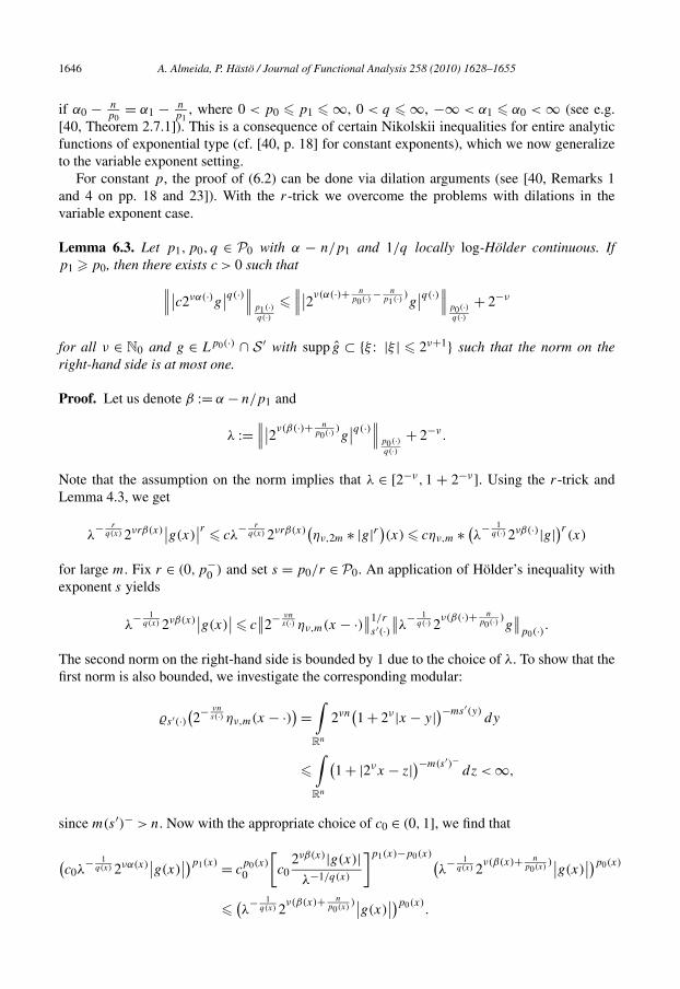
1646 A. Almeida, P. Hästö / Journal of Functional Analysis 258 (2010) 1628–1655
if α0 − np0
= α1 − np1
, where 0 < p0 � p1 � ∞, 0 < q � ∞, −∞ < α1 � α0 < ∞ (see e.g.[40, Theorem 2.7.1]). This is a consequence of certain Nikolskii inequalities for entire analyticfunctions of exponential type (cf. [40, p. 18] for constant exponents), which we now generalizeto the variable exponent setting.
For constant p, the proof of (6.2) can be done via dilation arguments (see [40, Remarks 1and 4 on pp. 18 and 23]). With the r-trick we overcome the problems with dilations in thevariable exponent case.
Lemma 6.3. Let p1,p0, q ∈ P0 with α − n/p1 and 1/q locally log-Hölder continuous. Ifp1 � p0, then there exists c > 0 such that∥∥∥∣∣c2να(·)g
∣∣q(·)∥∥∥ p1(·)q(·)
�∥∥∥∣∣2ν(α(·)+ n
p0(·) − np1(·) )g
∣∣q(·)∥∥∥ p0(·)q(·)
+ 2−ν
for all ν ∈ N0 and g ∈ Lp0(·) ∩ S ′ with supp g ⊂ {ξ : |ξ | � 2ν+1} such that the norm on theright-hand side is at most one.
Proof. Let us denote β := α − n/p1 and
λ :=∥∥∥∣∣2ν(β(·)+ n
p0(·) )g∣∣q(·)∥∥∥ p0(·)
q(·)+ 2−ν.
Note that the assumption on the norm implies that λ ∈ [2−ν,1 + 2−ν]. Using the r-trick andLemma 4.3, we get
λ− r
q(x) 2νrβ(x)∣∣g(x)
∣∣r � cλ− r
q(x) 2νrβ(x)(ην,2m ∗ |g|r)(x) � cην,m ∗ (
λ− 1
q(·) 2νβ(·)|g|)r(x)
for large m. Fix r ∈ (0,p−0 ) and set s = p0/r ∈ P0. An application of Hölder’s inequality with
exponent s yields
λ− 1
q(x) 2νβ(x)∣∣g(x)
∣∣ � c∥∥2− νn
s(·) ην,m(x − ·)∥∥1/r
s′(·)∥∥λ
− 1q(·) 2
ν(β(·)+ np0(·) )g
∥∥p0(·).
The second norm on the right-hand side is bounded by 1 due to the choice of λ. To show that thefirst norm is also bounded, we investigate the corresponding modular:
s′(·)(2− νn
s(·) ην,m(x − ·)) =∫Rn
2νn(1 + 2ν |x − y|)−ms′(y)
dy
�∫Rn
(1 + |2νx − z|)−m(s′)−
dz < ∞,
since m(s′)− > n. Now with the appropriate choice of c0 ∈ (0,1], we find that
(c0λ
− 1q(x) 2να(x)
∣∣g(x)∣∣)p1(x) = c
p0(x)
0
[c0
2νβ(x)|g(x)|λ−1/q(x)
]p1(x)−p0(x)(λ
− 1q(x) 2
ν(β(x)+ np0(x)
)∣∣g(x)∣∣)p0(x)
�(λ
− 1q(x) 2
ν(β(x)+ np0(x)
)∣∣g(x)∣∣)p0(x)
.

A. Almeida, P. Hästö / Journal of Functional Analysis 258 (2010) 1628–1655 1647
Integrating this inequality over Rn and taking into account the definition of λ gives us the
claim. �Applying the previous lemma, we obtain the following generalization of (6.2).
Theorem 6.4 (Sobolev inequality). Let p0,p1, q ∈ P0 and α0, α1 ∈ L∞ with α0 � α1. If 1/q and
α0(x) − n
p0(x)= α1(x) − n
p1(x)
are locally log-Hölder continuous, then
Bα0(·)p0(·),q(·) ↪→ B
α1(·)p1(·),q(·).
Proof. Suppose without loss of generality that the Bα0(·)p0(·),q(·)-modular of a function is less than 1.
Then an application of the previous lemma with α(x) = α1(x) and g = ϕν ∗ f , shows that theB
α1(·)p1(·),q(·)-modular is bounded by a constant. �
Corollary 6.5. Let p0,p1, q0, q1 ∈ P0 and α0, α1 ∈ L∞ with α0 � α1. If
α0(x) − n
p0(x)= α1(x) − n
p1(x)+ ε(x)
is locally log-Hölder continuous and ε− > 0, then
Bα0(·)p0(·),q0(·) ↪→ B
α1(·)p1(·),q1(·).
Proof. By Theorems 6.1(i) and 6.4,
Bα0(·)p0(·),q0(·) ↪→ B
α0(·)p0(·),∞ ↪→ B
α1(·)+ε(·)p1(·),∞ .
We combine this with the embedding Bα1(·)+ε(·)p1(·),∞ ↪→ B
α1(·)p1(·),q1(·) from Theorem 6.1(ii) to conclude
the proof. �Remark 6.6. It suffices to assume uniform continuity in the previous corollary (and hence inProposition 6.9) instead of log-Hölder continuity. This is achieved by choosing an auxiliarysmoothness function α between α0 and α1 with the appropriate continuity modulus.
Let Cu be the space of all bounded uniformly continuous functions on Rn equipped with the
sup norm. Concerning embeddings into Cu, we have the following result.
Corollary 6.7. Let α ∈ Clogloc , p ∈ P log and q ∈ P0. If
α(x) − n
p(x)� δ max
{1 − 1
q(x),0
}
for some fixed δ > 0 and every x ∈ Rn, then
Bα(·)p(·),q(·) ↪→ Cu.

1648 A. Almeida, P. Hästö / Journal of Functional Analysis 258 (2010) 1628–1655
Proof. Let γ (x) := α(x) − np(x)
. By Theorem 6.1(i), we may replace q with the larger exponent
max{1, δ/(δ − γ )} ∈ P log. It then follows from Theorem 6.4 that
Bα(·)p(·),q(·) ↪→ B
γ(·)∞,q(·).
Since B0∞,1 ↪→ Cu by classical results (e.g., [40, Proposition 2.5.7]), we will complete the proof
by showing that
Bγ(·)∞,q(·) ↪→ B0
∞,1.
Denote fν := ϕν ∗ f . The remaining embedding can be written, using homogeneity in theusual manner, as
∑ν
supx
|fν | � c whenever∑ν
supx
∣∣2νγ (x)fν
∣∣q(x) � 1,
where we used the expression from Example 3.2 for the second modular. We choose xν such thatsupx |fν | � 2|fν(xν)| for each ν. Then it follows from Young’s inequality that
∑ν
supx
|fν | ≈∑ν
∣∣fν(xν)∣∣ �
∑ν
∣∣2νγ (xν)fν(xν)∣∣q(xν) + 2−νγ (xν)q ′(xν) � 1 +
∑ν
2−νδ � c,
which completes the proof of the remaining embedding. �Let Lα,p(·), α ∈ R, be the Bessel potential space modeled in Lp(·). It was shown in [15] that
Fαp(·),2 = Lα,p(·) when α � 0, 1 < p− � p+ < ∞ and p ∈ P log. Under the same assumptions
on p, by Theorem 6.1 one gets the embedding
Bα(·)p(·),q(·) ↪→ Lσ,p(·)
for α− > σ � 0. In particular, we have Bα(·)p(·),q(·) ↪→ Lp(·) if α− > 0 (cf. [4, Corollary 6.2] or
[19, Theorem 6.1]). Next we derive a stronger version of this.Let us define
σp(x) := n
(1
min{1,p(x)} − 1
)and p(x) := max
{1,p(x)
}, x ∈ R
n. (6.8)
If α − n/p = α − σp − n/p is log-Hölder continuous, p,q ∈ P0, α ∈ L∞ and (α − σp)− > 0,then by Corollary 6.5 we get
Bα(·)p(·),q(·) ↪→ B0
p(·),1.
We further conclude that
‖f ‖p(·) �∑
‖ϕν ∗ f ‖p(·) = ‖f ‖B0p(·),1
� c‖f ‖B
α(·)−σp(·)p(·),1
.
ν�0

A. Almeida, P. Hästö / Journal of Functional Analysis 258 (2010) 1628–1655 1649
This shows that under the above assumptions the elements from Bα(·)p(·),q(·) are regular distribu-
tions. A discussion of such results for constant exponents can be found in [40, Section 2.5.3]; seealso [33, Section 2.2.4]. In sum, we obtain the following result, without the assumptions p− > 1and p+ < ∞.
Proposition 6.9. Assume that p,q ∈ P0 and α ∈ L∞ are such that α − n/p is log-Hölder con-tinuous. Let σp and p be as in (6.8). If (α − σp)− > 0, then
Bα(·)p(·),q(·) ↪→ Lp(·).
Let p,q ∈ P0 and α ∈ L∞. Define α0 := (α − np)−. Then α � α0 + n
p=: α1 ∈ L∞. It is clear
that α1 − np
= α0 is log-Hölder continuous. Therefore we obtain by Theorem 6.4 that
Bα(·)p(·),q(·) ↪→ B
α1(·)p(·),∞ ↪→ B
α1(·)− np(·)∞,∞ = Bα0∞,∞ ↪→ S ′.
Here the last embedding is just the well-known constant exponent case [40, Theorem 2.3.3].A similar argument gives the embedding of S into the variable index Besov space. Thus weobtain:
Theorem 6.10. If p,q ∈ P0 and α ∈ L∞, then
S ↪→ Bα(·)p(·),q(·) ↪→ S ′.
Remark 6.11. As in the classical case (e.g. [40, Theorem 2.3.3]), using the previous theorem onecan prove the completeness of the Besov space B
α(·)p(·),q , hence it is a (quasi)Banach space.
7. The Hölder–Zygmund space
In this section we show that our scale of Besov spaces includes also the Hölder–Zygmundspaces of continuous functions. This application requires in particular that we include the caseof unbounded p and q .
We start by generalizing the definition of Hölder–Zygmund spaces to the variable order set-ting. Such spaces have been considered e.g. in [5,6,32].
Recall that Cu denotes the set of all bounded uniformly continuous functions.
Definition 7.1. Let α : Rn → (0,1]. The Zygmund space Cα(·) consists of all f ∈ Cu such that‖f ‖Cα(·) < ∞, where
‖f ‖Cα(·) := ‖f ‖∞ + supx∈Rn,h∈Rn\{0}
|�2hf (x)|
|h|α(x).
For α < 1, the Hölder space Cα(·) is defined analogously but with the norm given by
‖f ‖Cα(·) := ‖f ‖∞ + supn n
|�1hf (x)|
|h|α(x).
x∈R ,h∈R \{0}

1650 A. Almeida, P. Hästö / Journal of Functional Analysis 258 (2010) 1628–1655
Here �jh is the j -th order difference operator (h ∈ R
n, j ∈ N):
�1hf (x) = f (x + h) − f (x), �
j+1h f = �1
h
(�
jhf
).
One can easily derive the point-wise inequality
suph
|h|−α(x)∣∣�1
hf (x)∣∣ � 1
2 − 2α+ suph
|h|−α(x)∣∣�2
hf (x)∣∣, x ∈ R
n.
Hence we have Cα(·) ↪→ Cα(·) for α+ < 1. In fact, these two spaces coincide for such α, as in theclassical case. This is one consequence of the following result.
Theorem 7.2. For α locally log-Hölder continuous with α− > 0,
Bα(·)∞,∞ = Cα(·) (α � 1) and Bα(·)∞,∞ = Cα(·) (α+ < 1
).
Combining this result with the embeddings from Section 6 as follows
W 1,p(·) = F 1p(·),2 ↪→ B1
p(·),∞ ↪→ B1−n/p(·)∞,∞ = C1−n/p(·),
we obtain the following result which extends [6, Theorem 7] to unbounded domains in the caseof Euclidean spaces.
Corollary 7.3. If p ∈ P log with n < p− � p+ < ∞, then
W 1,p(·) ↪→ C1−n/p(·).
By a similar argument, we can also obtain the embedding
Bα(·)+n/p(·)p(·),q(·) ↪→ Cα(·)
in the case α− > 0 for p,q ∈ P log0 and α ∈ C
logloc . We then move on to the proof of the theorem
itself.
Proof of Theorem 7.2. The proof is naturally divided into two parts. First we consider the claimthat
Cα(·) ↪→ Bα(·)∞,∞ (α � 1) and Cα(·) ↪→ Bα(·)∞,∞(α+ < 1
).
We prove only the first embedding; the second is similar. We estimate the absolute value on theright-hand side of
‖f ‖B
α(·)∞,∞= sup
νsupx
∣∣2να(x)ϕν ∗ f (x)∣∣
by ‖f ‖Cα(·) . The term ν = 0 is easily estimated in terms of ‖f ‖∞, so we consider in what followsν > 0.

A. Almeida, P. Hästö / Journal of Functional Analysis 258 (2010) 1628–1655 1651
Since the Besov space is independent of the choice of admissible ϕ, we may assume withoutloss of generality that ϕ(−y) = ϕ(y). Then
ϕν ∗ f (x) = 1
2
∫Rn
ϕν(h)[f (x + h) + f (x − h)
]dh = 1
2
∫Rn
ϕν(h)�2hf (x − h)dh,
where we used the fact that∫
ϕν(y) dy = ϕν(0) = 0 in the second step. By definition,|�2
hf (x−h)| � ‖f ‖Cα(·) |h|α(x−h). For small h, the log-Hölder continuity implies that |h|α(x−h) �c|h|α(x). Thus we obtain
∣∣ϕν ∗ f (x)∣∣ � c
∫|h|<1
∣∣ϕν(h)∣∣|h|α(x) dh + c
∫|h|�1
∣∣ϕν(h)∣∣|h|α+
dh
= c
∫|h|<2ν
∣∣ϕ(h)∣∣∣∣2−νh
∣∣α(x)dh + c
∫|h|�2ν
∣∣ϕ(h)∣∣∣∣2−νh
∣∣α+dh
� c2−να(x)
∫Rn
∣∣ϕ(h)∣∣[|h|α+ + |h|α−]
dh,
where in the second step we used a change of variables. Since ϕ decays faster than any polyno-mial (as supp ϕ is bounded), the integral on the right-hand side is finite, and so we are done.
We then move on to the second part of the proof of the theorem, and consider the claim
Bα(·)∞,∞ ↪→ Cα(·) (α � 1) and Bα(·)∞,∞ ↪→ Cα(·) (α+ < 1
).
First we note that
sup0<|h|�1
supx
|�Mh f (x)||h|α(x)
� 2α+supk�0
sup|h|�2−k
supx
∣∣2kα(x)�Mh f (x)
∣∣.(We restrict ourselves to |h| � 1 since large h are easily handled.) For a > 0 and M � 1 thereexists c > 0 such that
∣∣�Mh (ϕν ∗ f )(x)
∣∣ � c min{1,2(ν−k)M
}(ϕ∗
ν f)a(x),
for every ν, k ∈ N0 and |h| � 2−k , where (ϕ∗ν f )a(x) := supy
|ϕν∗f (x−y)|1+|2νy|a is the Peetre maximal
function, cf. [40, (2.5.12/8)]. Since f = ∑ν ϕν ∗ f with convergence in L∞, we can use the
previous estimate to obtain
sup|h|�2−k
∣∣2kα(x)�Mh f (x)
∣∣ � c∑ν<k
2(ν−k)(M−α(x))2να(x)(ϕ∗
ν f)a(x)
+ c∑
2(k−ν)α(x)2να(x)(ϕ∗
ν f)a(x). (7.4)
ν�k+1

1652 A. Almeida, P. Hästö / Journal of Functional Analysis 258 (2010) 1628–1655
Therefore, we need to estimate 2να(x)(ϕ∗ν f )a(x). Let us denote K := supx 2να(x)|ϕν ∗ f (x)|.
Then
2να(x)(ϕ∗
ν f)a(x) = sup
y2να(x) |ϕν ∗ f (x − y)|
1 + |2νy|a � K supy
2ν(α(x)−α(x−y))
1 + |2νy|a .
When |y| < 2−ν/2, it follows from the log-Hölder continuity of α that ν(α(x) − α(x − y)) � c.When |y| � 2−ν/2, the right-hand side is bounded by K2ν(α+−α−−a/2), which remains boundedprovided we choose a > 2(α+ − α−). Therefore we have shown that
2να(x)(ϕ∗
ν f)a(x) � c sup
x2να(x)
∣∣ϕν ∗ f (x)∣∣ � c‖f ‖
Bα(·)∞,∞
.
Using this in (7.4), we find that
sup|h|�2−k
∣∣2kα(x)�Mh f (x)
∣∣ � c
[ ∑ν<k
2(ν−k)(M−α+) +∑
ν�k+1
2(k−ν)α−]‖f ‖
Bα(·)∞,∞
.
If M = 1, then we have assumed that α+ < 1; for M = 2, M − α+ � 1. Thus the terms inthe brackets are bounded, so we have estimated the main part of the norm. Since we also have‖f ‖∞ � c‖f ‖
Bα(·)∞,∞
for α− > 0, the proof is complete. �8. Characterization by approximations
The aim of this section is to characterize the elements from Bα(·)p(·),q(·) in terms of Nikolskii
representations involving sequences of entire analytic functions. Let
U p(·) := {(uν)ν ⊂ S ′ ∩ Lp(·): supp uν ⊂ {
ξ : |ξ | � 2ν+1}, ν ∈ N0}.
Theorem 8.1. Let p,q ∈ P log0 and α ∈ C
logloc ∩L∞ with α− > 0. Then f ∈ S ′ belongs to B
α(·)p(·),q(·)
if and only if there exists u = (uν)ν ∈ U p(·) such that
f = limν→∞uν in S ′ (8.2)
and
‖f ‖u := ‖u0‖p(·) + ∥∥(2να(·)(f − uν)
)ν
∥∥q(·)(Lp(·))�
< ∞.
Moreover,
‖f ‖� := infu
‖f ‖u
is an equivalent quasinorm in Bα(·)p(·),q(·), where the infimum is taken over all possible representa-
tions (uν)ν ∈ U p(·) satisfying (8.2).

A. Almeida, P. Hästö / Journal of Functional Analysis 258 (2010) 1628–1655 1653
Proof. First we show that ‖f ‖� � c‖f ‖B
α(·)p(·),q(·)
. If (ϕν)ν is an admissible system, then
uν :=ν∑
j=0
ϕj ∗ f → f in S ′ as ν → ∞.
Thus (uν)ν ∈ U p(·) and
(2να(·)(f − uν)
)ν=
∑j�0
2−jα(·)(2(j+ν)α(·)ϕj+ν ∗ f)ν
in S ′.
Observe that 2−jα(·) � 2−jα−and that α− > 0 by assumption. Let r ∈ (0, 1
2 min{p,q,2}). Us-ing the previous expression and the triangle inequality in the mixed Lebesgue-sequence space(Theorem 3.6), we obtain
∥∥(2να(·)(f − uν)
)ν
∥∥�q(·)(Lp(·)) =
∥∥∥∥∣∣∣∣∑j�0
2−jα(·)(2(j+ν)α(·)ϕj+ν ∗ f)ν
∣∣∣∣r∥∥∥∥
1r
�q(·)r (L
p(·)r )
�∥∥∥∥ ∑
j�0
2−jrα(·)(2(j+ν)rα(·)|ϕj+ν ∗ f |r)ν
∥∥∥∥1r
�q(·)r (L
p(·)r )
�( ∑
j�0
2−jrα−∥∥(2(j+ν)rα(·)|ϕj+ν ∗ f |r)
ν
∥∥�
q(·)r (L
p(·)r )
) 1r
� c∥∥(
2να(·)ϕν ∗ f)ν
∥∥�q(·)(Lp(·)),
where the last step follows from the invariance of the norm under shifts in the ν direction. Since‖u0‖p(·) = ‖ϕ0 ∗ f ‖p(·) � ‖f ‖
Bα(·)p(·),q(·)
, we have shown that
‖f ‖u � c‖f ‖B
α(·)p(·),q(·)
.
Now we prove the opposite inequality. Let (uk)k ∈ U p(·) be such that f = limk→∞ uk and‖f ‖u < ∞. Then ϕν ∗ f = ∑
k�−1 ϕν ∗ (uν+k − uν+k−1), ν ∈ N0 (with u−1 = 0). Using ther-trick, with r as before, we find that
2να(x)|ϕν ∗ f | � 2να(x)∑
k�−1
∣∣ϕν ∗ (uν+k − uν+k−1)∣∣
�∑
k�−1
[ην,m ∗ (
2να(·)r |uν+k − uν+k−1|r)] 1
r .
Since 2να(·) � 2(ν+k)α(·)2−kα−, we obtain

1654 A. Almeida, P. Hästö / Journal of Functional Analysis 258 (2010) 1628–1655
∥∥(2να(·)ϕν ∗ f
)ν
∥∥�q(·)(Lp(·))
� c∑
k�−1
2−kα−∥∥(ην,m ∗ (
2(ν+k)α(·)r |uν+k − uν+k−1|r))
ν
∥∥ 1r
�q(·)r (L
p(·)r )
.
Then we can get rid of the function η by Lemma 4.7. Using
|uν+k − uν+k−1| � |f − uν+k| + |f − uν+k−1|,we find that∥∥(
2να(·)ϕν ∗ f)ν
∥∥�q(·)(Lp(·)) � c
∑k�−1
2−kα−∥∥(2(ν+k)α(·)(f − uν+k)
)ν
∥∥�q(·)(Lp(·)).
Using again the invariance of the sequence space with respect to shifts, we see that the left-hand side can be estimated by a constant times ‖f ‖u. Taking the infimum over u, we obtain‖f ‖
Bα(·)p(·),q(·)
� c‖f ‖�. �Remark 8.3. Compared to the proof given in [40, Theorem 2.5.3] for constant exponents, weused the r-trick to circumvent the use of Fourier multipliers. Consequently, our proof requiresonly the assumption α− > 0, while the stronger assumption α > σp is needed in [40] even in theconstant exponent case.
References
[1] E. Acerbi, G. Mingione, Regularity results for a class of functionals with nonstandard growth, Arch. Ration. Mech.Anal. 156 (2) (2001) 121–140.
[2] E. Acerbi, G. Mingione, Regularity results for stationary electro-rheological fluids, Arch. Ration. Mech.Anal. 164 (3) (2002) 213–259.
[3] E. Acerbi, G. Mingione, Gradient estimates for the p(x)-Laplacian system, J. Reine Angew. Math. 584 (2005)117–148.
[4] A. Almeida, S. Samko, Characterization of Riesz and Bessel potentials on variable Lebesgue spaces, J. Funct.Spaces Appl. 4 (2) (2006) 113–144.
[5] A. Almeida, S. Samko, Pointwise inequalities in variable Sobolev spaces and applications, Z. Anal. Anwend. 26 (2)(2007) 179–193.
[6] A. Almeida, S. Samko, Embeddings of variable Hajłasz–Sobolev spaces into Hölder spaces of variable order,J. Math. Anal. Appl. 353 (2) (2009) 489–496.
[7] A. Beauzamy, Espaces de Sobolev et Besov d’ordre variable définis sur Lp , C. R. Acad. Sci. Paris Ser. A 274 (1972)1935–1938.
[8] O. Besov, On spaces of functions of variable smoothness defined by pseudodifferential operators, Tr. Mat. Inst.Steklova 227 (1999), Issled. po Teor. Differ. Funkts. Mnogikh Perem. i ee Prilozh. 18, 56–74, translation in: Proc.Steklov Inst. Math. 4 (227) (1999) 50–69.
[9] O. Besov, Equivalent normings of spaces of functions of variable smoothness, Tr. Mat. Inst. Steklova 243 (2003)(in Russian), Funkts. Prostran., Priblizh., Differ. Uravn., 87–95, translation in: Proc. Steklov Inst. Math. 243 (4)(2003) 80–88.
[10] O. Besov, Interpolation, embedding, and extension of spaces of functions of variable smoothness, Tr. Mat. Inst.Steklova 248 (2005) (in Russian), Issled. po Teor. Funkts. i Differ. Uravn., 52–63, translation in: Proc. Steklov Inst.Math. 248 (1) (2005) 47–58.
[11] Y. Chen, S. Levine, R. Rao, Variable exponent, linear growth functionals in image restoration, SIAM J. Appl.Math. 66 (4) (2006) 1383–1406.
[12] D. Cruz-Uribe, A. Fiorenza, J.M. Martell, C. Pérez, The boundedness of classical operators in variable Lp spaces,Ann. Acad. Sci. Fenn. Math. 13 (2006) 239–264.
[13] L. Diening, P. Harjulehto, P. Hästö, M. Ružicka, Variable Exponent Function Spaces, 2009, book manuscript.

A. Almeida, P. Hästö / Journal of Functional Analysis 258 (2010) 1628–1655 1655
[14] L. Diening, P. Hästö, A. Nekvinda, Open problems in variable exponent Lebesgue and Sobolev spaces, in: P. Drabek,J. Rákosník (Eds.), FSDONA04 Proceedings, Milovy, Czech Republic, Czech Academy of Sciences, 2004, pp. 38–58.
[15] L. Diening, P. Hästö, S. Roudenko, Function spaces of variable smoothness and integrability, J. Funct. Anal. 256 (6)(2009) 1731–1768.
[16] X.-L. Fan, Global C1,α regularity for variable exponent elliptic equations in divergence form, J. Differential Equa-tions 235 (2) (2007) 397–417.
[17] W. Farkas, H.-G. Leopold, Characterisations of function spaces of generalised smoothness, Ann. Mat. PuraAppl. 185 (1) (2006) 1–62.
[18] R. Fortini, D. Mugnai, P. Pucci, Maximum principles for anisotropic elliptic inequalities, Nonlinear Anal. 70 (8)(2009) 2917–2929.
[19] P. Gurka, P. Harjulehto, A. Nekvinda, Bessel potential spaces with variable exponent, Math. Inequal. Appl. 10 (3)(2007) 661–676.
[20] P. Harjulehto, P. Hästö, V. Latvala, Minimizers of the variable exponent, non-uniformly convex Dirichlet energy,J. Math. Pures Appl. (9) 89 (2) (2008) 174–197.
[21] P. Harjulehto, P. Hästö, Ú. Lê, M. Nuortio, Overview of differential equations with non-standard growth, preprint,2009.
[22] W. Hoh, Pseudo differential operators with negative definite symbols of variable order, Rev. Mat. Iberoameri-cana 16 (2) (2000) 219–241.
[23] H. Kempka, 2-Microlocal Besov and Triebel–Lizorkin spaces of variable integrability, Rev. Mat. Complut. 22 (1)(2009) 227–251.
[24] O. Kovácik, J. Rákosník, On spaces Lp(x) and W1,p(x) , Czechoslovak Math. J. 41 (116) (1991) 592–618.[25] H.-G. Leopold, On Besov spaces of variable order of differentiation, Z. Anal. Anwend. 8 (1) (1989) 69–82.[26] H.-G. Leopold, On function spaces of variable order of differentiation, Forum Math. 3 (1991) 633–644.[27] H.-G. Leopold, Embedding of function spaces of variable order of differentiation in function spaces of variable
order of integration, Czechoslovak Math. J. 49(124) (3) (1999) 633–644.
[28] T. Ohno, Compact embeddings in the generalized Sobolev space W1,p(·)0 (G) and existence of solutions for nonlinear
elliptic problems, Nonlinear Anal. 71 (5–6) (2009) 1535–1541.[29] W. Orlicz, Über konjugierte Exponentenfolgen, Studia Math. 3 (1931) 200–212.[30] G. Mingione, Regularity of minima: An invitation to the dark side of the calculus of variations, Appl. Math. 51
(2006) 355–425.[31] J. Musielak, Orlicz Spaces and Modular Spaces, Lecture Notes in Math., vol. 1034, Springer-Verlag, Berlin, 1983.[32] B. Ross, S. Samko, Fractional integration operator of variable order in the spaces Hλ, Int. J. Math. Sci. 18 (4) (1995)
777–788.[33] T. Runst, W. Sickel, Sobolev Spaces of Fractional Order, Nemytskij Operators and Nonlinear Partial Differential
Equations, de Gruyter Ser. Nonlinear Anal. Appl., vol. 3, Walter de Gruyter, Berlin, 1996.[34] M. Ružicka, Electrorheological Fluids, Modeling and Mathematical Theory, Lecture Notes in Math., vol. 1748,
Springer-Verlag, Berlin, 2000.[35] M. Sanchón, J.M. Urbano, Entropy solutions for the p(x)-Laplace equation, Trans. Amer. Math. Soc. 361 (2009)
6387–6405.[36] S. Samko, On a progress in the theory of Lebesgue spaces with variable exponent: Maximal and singular operators,
Integral Transforms Spec. Funct. 16 (5-6) (2005) 461–482.[37] J. Schneider, Function spaces of varying smoothness, I, Math. Nachr. 280 (16) (2007) 1801–1826.[38] J. Schneider, Some results on function spaces of varying smoothness, Banach Center Publ. 79 (2008) 187–195.[39] R. Schneider, C. Schwab, Wavelet solution of variable order pseudodifferential equations, preprint, 2006.[40] H. Triebel, Theory of Function Spaces, Monogr. Math., vol. 78, Birkhäuser Verlag, Basel, 1983.[41] H. Triebel, Theory of Function Spaces, II, Monogr. Math., vol. 84, Birkhäuser Verlag, Basel, 1992.[42] H. Triebel, Theory of Function Spaces, III, Monogr. Math., vol. 100, Birkhäuser Verlag, Basel, 2006.[43] J. Vybíral, Sobolev and Jawerth embeddings for spaces with variable smoothness and integrability, Ann. Acad. Sci.
Fenn. Math. 34 (2) (2009) 529–544.[44] J.-S. Xu, Variable Besov and Triebel–Lizorkin spaces, Ann. Acad. Sci. Fenn. Math. 33 (2008) 511–522.[45] J.-S. Xu, The relation between variable Bessel potential spaces and Triebel–Lizorkin spaces, Integral Transforms
Spec. Funct. 19 (8) (2008) 599–605.[46] J.-S. Xu, An atomic decomposition of variable Besov and Triebel–Lizorkin spaces, Armenian J. Math. 2 (1) (2009)
1–12.[47] Q.-H. Zhang, X.-P. Liu, Z.-M. Qiu, On the boundary blow-up solutions of p(x)-Laplacian equations with singular
coefficient, Nonlinear Anal. 70 (11) (2009) 4053–4070.


![Uniform convexity and smoothness, and their applications ...sohta/papers/Funi.pdf · the geometry of Banach spaces. We refer to [BCS], [Eg], [Sh1], [Sh2], [Sh3] and [WX] for known](https://img.pdfslide.us/doc/110x75/5edb03b009ac2c67fa68ab72/uniform-convexity-and-smoothness-and-their-applications-sohtapapersfunipdf.jpg)

![Superposition operators and functions of bounded p ... · superposition operators in function spaces with positive smoothness, see [9] for further details. What also contributes to](https://img.pdfslide.us/doc/110x75/607c12cae867a13f944d4e76/superposition-operators-and-functions-of-bounded-p-superposition-operators-in.jpg)