Beneﬁts and challenges of over-actuated excitation systems

Shock and Vibration 17 (2010) 285–303 285DOI 10.3233/SAV-2010-0513IOS Press

Benefits and challenges of over-actuatedexcitation systems

Norman Fitz-Coya, Vivek Nagabhushana and Michael T. Haleb,∗aDepartment of Mechanical and Aerospace Engineering, University of Florida, FL, USAbDynamic Test Branch, Redstone Technical Test Center, U.S. Army Developmental Test Command, USA

Abstract. This paper provides a comprehensive discussion on the benefits and technical challenges of controlling over-determinedand over-actuated excitation systems ranging from 1-DOF to 6-DOF. The primary challenges of over-actuated systems resultfrom the physical constraints imposed when the number of exciters exceeds the number of mechanical degree-of-freedom. Thisissue is less critical for electro-dynamic exciters which tend to be more compliant than servo-hydraulic exciters. To facilitate thetechnical challenges discussion, generalized methods for determining the drive output commands and the actuator input transformis presented. To further provide insights into the problem, over-actuated 1-DOF and 6-DOF examples are provided. Results arepresented to support the discussions.

1. Introduction

Dynamic testing in a laboratory environment has long been a successful method of experimentally determiningthe mechanical properties of a structure as well as a technique for providing a degree of confidence that the unitunder test (UUT) can structurally and functionally withstand a specified deployment environment. The simplestand most common laboratory vibration test consists of a single exciter providing motion in a single mechanicaldegree-of-freedom. However, there are many circumstances that will require use of multiple exciters to meet testobjectives. A multiple exciter test (MET) is required whenever more than one mechanical degree-of freedom isrequired simultaneously, when a single actuator is not capable of addressing the test requirement, or possibly acombination of both scenarios. Clearly, one could envision unlimited combinations of actuator placements, actuatorperformance, and payload combinations.

The use of MET has overlap into different disciplines including the automotive, aerospace, defense, and seismiccommunities [1–21]. Much of the early application of over-actuated 6-DOF excitation systems can be traced backto the seismic community. The designs were typically addressing very large payloads such as buildings or bridgestructures with test bandwidths of interest generally in the DC to 50 Hz range. In recent years, the application ofMET has become more wide-spread in the general dynamic test community yielding numerous systems with widelyvarying size and operational bandwidths. Many existing MET configurations are not over-actuated and control ofthese systems has been successful using a variety of commercially available control systems. Of primary interest,and the basis for the discussions within this paper, are the challenges associated with high bandwidth over-actuatedMET configurations. Particular attention will be paid to the unique issues presented when designing and controllingwide bandwidth (up to 500 Hz) over-actuated servo-hydraulic systems.

This paper is outlined as follows. First we motivate the need for over-actuated METs which is followed by ananalysis of the kinematic constraints that are imposed by such systems. These discussions are followed by specificexamples to highlight the characteristics of these systems. Finally we close with some recommendations for thecommunity to consider.

∗Corresponding author. E-mail: [email protected].

ISSN 1070-9622/10/$27.50 2010 – IOS Press and the authors. All rights reserved

286 N. Fitz-Coy et al. / Benefits and challenges of over-actuated excitation systems

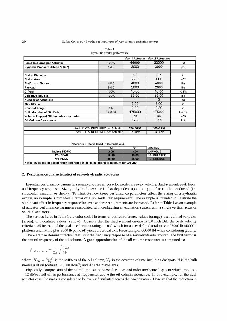
Table 1Hydraulic exciter performance

Vert-1 Actuator Vert-2 Actuators

Force Required per Actuator 100% 66000 33000 lbfDynamic Pressure (Static *0.667) 4500 3000 3000 psi

Piston Diameter 5.3 3.7 inPiston Area 22.0 11.0 in^2Platform + Fixture 4000 4000 4000 lbsPayload 2000 2000 2000 lbsG-Peak 100% 10.00 10.00 G-PkVelocity Required 100% 35.00 35.00 ipsNumber of Actuators 1 2 eaMax Stroke 3.00 3.00 inDashpot Length 5% 0.30 0.30 inBulk Modulus of Oil (Beta) 175000 175000 175000 lb/in^2Volume Trapped Oil (includes dashpots) 73 36 in^3Oil Column Resonance 87.2 87.2 Hz

Peak FLOW REQUIRED per Actuator 200 GPM 100 GPMRMS FLOW REQUIRED per Actuator 67 GPM 33 GPM

V2 V1 LEGEND:Inches PK-PK 3.00 3.00 VARIABLE

G’s PEAK 10.00 10.00 CALCULATEDV’s PEAK 35.00 35.00 REFERENCE

Note: 1G added ot acceleration reference in all calculations to account for Gravity.

Reference Criteria Used in Calculations

2. Performance characteristics of servo-hydraulic actuators

Essential performance parameters required to size a hydraulic exciter are peak velocity, displacement, peak force,and frequency response. Sizing a hydraulic exciter is also dependent upon the type of test to be conducted (i.e.sinusoidal, random, or shock). To illustrate how these performance parameters affect the sizing of a hydraulicexciter, an example is provided in terms of a sinusoidal test requirement. The example is intended to illustrate thesignificant effect in frequency response incurred as force requirements are increased. Refer to Table 1 as an exampleof actuator performance parameters associated with configuring an excitation system with a single vertical actuatorvs. dual actuators.

The various fields in Table 1 are color coded in terms of desired reference values (orange), user defined variables(green), or calculated values (yellow). Observe that the displacement criteria is 3.0 inch DA, the peak velocitycriteria is 35 in/sec, and the peak acceleration rating is 10 G which for a user defined total mass of 6000 lb (4000 lbplatform and fixture plus 2000 lb payload) yields a vertical axis force rating of 66000 lbf when considering gravity.

There are two dominant factors that limit the frequency response of a servo-hydraulic exciter. The first factor isthe natural frequency of the oil column. A good approximation of the oil column resonance is computed as:

fnoil column=

12π

√Koil

MT

where, Koil = 4βA2

VTis the stiffness of the oil column, VT is the actuator volume including dashpots, β is the bulk

modulus of oil (default 175,000 lb/in2) and A is the piston area.Physically, compression of the oil column can be viewed as a second order mechanical system which implies a

−12 db/oct roll-off in performance at frequencies above the oil column resonance. In this example, for the dualactuator case, the mass is considered to be evenly distributed across the two actuators. Observe that the reduction in

N. Fitz-Coy et al. / Benefits and challenges of over-actuated excitation systems 287

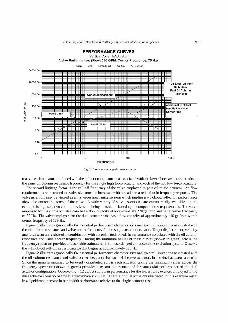
PERFORMANCE CURVESVertical Axis: 1-Actuator

Valve Performance: (Flow: 220 GPM, Corner Frequency: 75 Hz)

0.01

0.10

1.00

10.00

100.00

1000.00

10000.00

100000.00

1 10 100 1000FREQUENCY (Hz)

AC

CE

LE

RA

TIO

N (

G)

Disp Vel Force Limit Oil Col V_Corner

Const Displacement

Const Pk Vel

-12 dB/oct Vel Perf Reduction

Past Oil ColumnResonance

Force Limit

Additional -6 dB/oct Perf Red at Valve Corner Freq

Fig. 1. Single actuator performance curves.

mass at each actuator, combined with the reduction in piston area associated with the lower force actuators, results inthe same oil column resonance frequency for the single high force actuator and each of the two low force actuators.

The second limiting factor is the roll-off frequency of the valve employed to port oil to the actuator. As flowrequirements are increased the valve size must be increased which results in a reduction in frequency response. Thevalve assembly may be viewed as a first order mechanical system which implies a −6 db/oct roll-off in performanceabove the corner frequency of the valve. A wide variety of valve assemblies are commercially available. In theexample being used, two common valves are being considered based upon computed flow requirements. The valveemployed for the single actuator case has a flow capacity of approximately 220 gal/min and has a corner frequencyof 75 Hz. The valve employed for the dual actuator case has a flow capacity of approximately 110 gal/min with acorner frequency of 175 Hz.

Figure 1 illustrates graphically the essential performance characteristics and spectral limitations associated withthe oil column resonance and valve corner frequency for the single actuator scenario. Target displacement, velocityand force targets are plotted in combination with the estimated roll-off in performance associated with the oil columnresonance and valve corner frequency. Taking the minimum values of these curves (shown in green) across thefrequency spectrum provides a reasonable estimate of the sinusoidal performance of the excitation system. Observethe −12 db/oct roll-off in performance that begins at approximately 180 Hz.

Figure 2 illustrates graphically the essential performance characteristics and spectral limitations associated withthe oil column resonance and valve corner frequency for each of the two actuators in the dual actuator scenario.Since the mass is assumed to be evenly distributed across each actuator, taking the minimum values across thefrequency spectrum (shown in green) provides a reasonable estimate of the sinusoidal performance of the dualactuator configuration. Observe the −12 db/oct roll-off in performance for the lower force exciters employed in thedual actuator scenario begins at approximately 280 Hz. The use of dual actuators illustrated in this example resultin a significant increase in bandwidth performance relative to the single actuator case.


PERFORMANCE CURVESVertical Axis: 2-Actuators

Valve Performance: (Flow: 110 GPM, Corner Frequency: 175 Hz)

0.01

0.10

1.00

10.00

100.00

1000.00

10000.00

100000.00

1 10 100 1000FREQUENCY (Hz)

AC

CE

LE

RA

TIO

N (

G)

Disp Vel Force Limit Oil Col V_Corner

Const Displacement

Const Pk Vel

-12 dB/oct Vel Perf Reduction

past oil columnresonance

Force Limit

Additional -6 dB Perf Reduction at Valve Corner Freq

Fig. 2. Dual actuator performance curves.

The discussion within this section has been limited strictly to actuator performance. Omitted thus far are thedetails as to how multiple exciters may be configured. In the simple example provided, the two actuators couldbe configured, with proper mechanical constraints, such that either one or two mechanical degrees of freedom arepossible. For the case in which two mechanical degrees-of-freedom are possible, control is readily achievable viamultiple commercially available MDOF vibration control software products. The over-actuated cases in which thetwo hydraulic actuators are configured to obtain a single mechanical degree-of freedom introduce additional controlconcerns. It is the general over-actuated case employing hydraulic actuators that is the main subject of the sectionsthat follow.

3. Implementation considerations for over-determined and over-actuated excitation systems

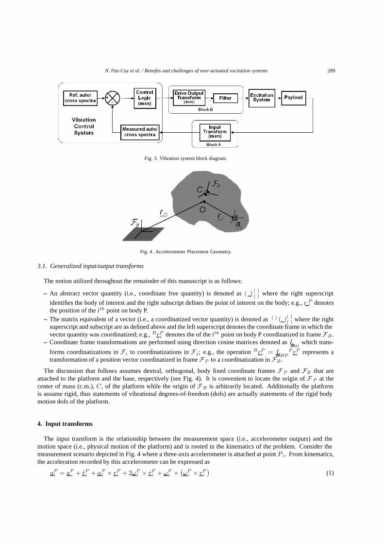
Consider a typical MET vibration system with d actuators, n measurements, and m motion degrees-of-freedom(DOFs). A block diagram of a typical MET vibration system is shown in Fig. 3. For the traditional single-degree-of-freedom system, blocks A and B would simply be unity and not exist. For the over-determined case, the number ofmeasurements (accelerometer output channels) exceeds the number of motion DOFs of the system (i.e., n > m) andthus requires a method for extracting the motion information from the measurements. This process is shown in BlockA and is referred to as “input” transform” in the literature [4]. Similarly for the over-actuated case, the excitationsystem contains more actuators that motion DOF (i.e. d > m), implying the need for coordination between theactuators. This process is referred to as “drive output transform” in the literature [4] and is shown as Block B inFig. 3.

The discussions below are intended to provide a unified approach to develop the input and drive output transformsdiscussed in Ref. [4]. Furthermore, these discussions should provide the vibration control engineer some physicalinsights into the mechanics of the problem and thus to potential solutions.


Fig. 3. Vibration system block diagram.

Fig. 4. Accelerometer Placement Geometry.

3.1. Generalized input/output transforms

The notion utilized throughout the remainder of this manuscript is as follows:

– An abstract vector quantity (i.e., coordinate free quantity) is denoted as ( ) ( )( ) where the right superscript

identifies the body of interest and the right subscript defines the point of interest on the body; e.g., r Pi denotes

the position of the ith point on body P.– The matrix equivalent of a vector (i.e., a coordinatized vector quantity) is denoted as ( ) ( )( )

( ) where the rightsuperscript and subscript are as defined above and the left superscript denotes the coordinate frame in which thevector quantity was coordinatized; e.g., BrPi denotes the of the ith point on body P coordinatized in frame FB .

– Coordinate frame transformations are performed using direction cosine matrices denoted as Lji

which trans-

forms coordinatizations in Fi to coordinatizations in Fj ; e.g., the operation BrPi = LBP

P rPi represents atransformation of a position vector coordinatized in frame FP to a coordinatization in FB .

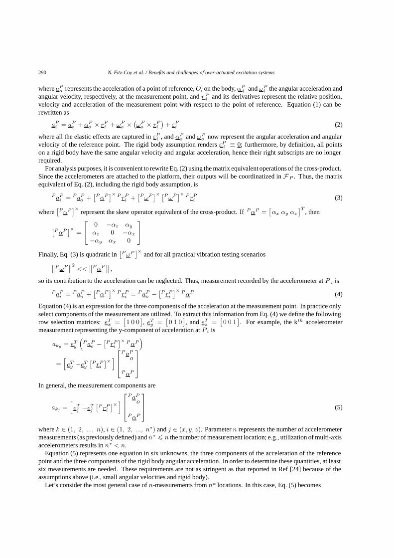
The discussion that follows assumes dextral, orthogonal, body fixed coordinate frames F P and FB that areattached to the platform and the base, respectively (see Fig. 4). It is convenient to locate the origin of F P at thecenter of mass (c.m.), C, of the platform while the origin of FB is arbitrarily located. Additionally the platformis assume rigid, thus statements of vibrational degrees-of-freedom (dofs) are actually statements of the rigid bodymotion dofs of the platform.

4. Input transforms

The input transform is the relationship between the measurement space (i.e., accelerometer outputs) and themotion space (i.e., physical motion of the platform) and is rooted in the kinematics of the problem. Consider themeasurement scenario depicted in Fig. 4 where a three-axis accelerometer is attached at point P i. From kinematics,the acceleration recorded by this accelerometer can be expressed as

aPi = aPo + rPi + αPi × rPi + 2ωP

i × rPi + ωPi × (

ωPi × rPi

)(1)


where aPo represents the acceleration of a point of reference, O, on the body, αPi and ωP

i the angular acceleration andangular velocity, respectively, at the measurement point, and r P

i and its derivatives represent the relative position,velocity and acceleration of the measurement point with respect to the point of reference. Equation (1) can berewritten as

aPi = aPo + αPo × rPi + ωP

o × (ωPo × rPi

)+ εPi (2)

where all the elastic effects are captured in εPi , and αPo and ωP

o now represent the angular acceleration and angularvelocity of the reference point. The rigid body assumption renders εPi ≡ 0; furthermore, by definition, all pointson a rigid body have the same angular velocity and angular acceleration, hence their right subscripts are no longerrequired.

For analysis purposes, it is convenient to rewrite Eq. (2) using the matrix equivalent operations of the cross-product.Since the accelerometers are attached to the platform, their outputs will be coordinatized in F P . Thus, the matrixequivalent of Eq. (2), including the rigid body assumption, is

PaPi = P aPo +[PαP

]× P rPi +[PωP

]× [PωP

]× P rPi (3)

where[PαP

]×represent the skew operator equivalent of the cross-product. If PαP =

[αx αy αz

]T, then

[PαP

]×=

0 −αz αy

αz 0 −αx

−αy αx 0

Finally, Eq. (3) is quadratic in[PωP

]×and for all practical vibration testing scenarios∥∥PωP

∥∥2<<

∥∥PαP∥∥ ,

so its contribution to the acceleration can be neglected. Thus, measurement recorded by the accelerometer at P i is

PaPi = P aPo +[PαP

]× P rPi = PaPo − [P rPi

]× PαP (4)

Equation (4) is an expression for the three components of the acceleration at the measurement point. In practice onlyselect components of the measurement are utilized. To extract this information from Eq. (4) we define the followingrow selection matrices: eTx =

[1 0 0

], eTy =

[0 1 0

], and eTz =

[0 0 1

]. For example, the kth accelerometer

measurement representing the y-component of acceleration at P i is

aky = eTy

(P aPo − [

P rPi]× PαP

)

=[eTy −eTy

[P rPi

]× ]

PaPo

PαP

In general, the measurement components are

akj =[eTj −eTj

[P rPi

]× ]

PaPo

PαP

(5)

where k ∈ (1, 2, ..., n), i ∈ (1, 2, ..., n∗) and j ∈ (x, y, z). Parameter n represents the number of accelerometermeasurements (as previously defined) and n∗ � n the number of measurement location; e.g., utilization of multi-axisaccelerometers results in n∗ < n.

Equation (5) represents one equation in six unknowns, the three components of the acceleration of the referencepoint and the three components of the rigid body angular acceleration. In order to determine these quantities, at leastsix measurements are needed. These requirements are not as stringent as that reported in Ref [24] because of theassumptions above (i.e., small angular velocities and rigid body).

Let’s consider the most general case of n-measurements from n* locations. In this case, Eq. (5) becomes


[akj

]=

a1j

a2j

...anj

(n×1)

=

eTj −eTj[P rP1

]×eTj −eTj

[P rPi

]×...

...

eTj −eTj[P rPn∗

]×

(n×6)

PaPo

PαP

(6×1)

, i ∈ (1, 2, ..., n∗) , j ∈ (x, y, z)

which is of the form

[A]meas(n×1)

=[I]

(n×6)

[A]motion(6×1)

(6)

Equation (6) can be rewritten as

[A]motion = [I] [A]meas (7)

where [A]motion is a 6x1 matrix of unknown linear and angular accelerations, [A]meas is an n× 1 matrix ofmeasurements (known), and [I] is a 6 ×n matrix referred to in the literature as the “Input Transform”.

Observe that[I]

is entirely defined by knowledge of (i) placement, (ii) orientation, and (iii) utilized signals of theaccelerometers. Since

[I] =([I]T [I])−1 [I]T

,

the Input Transform can always be determined provided[I]

has full column rank, which is entirely dependent onthe placement of the accelerometers. For example,

[I]will be rank deficient if accelerometers providing z-axis

outputs are positioned such that the x- and y-components of their position vectors are identical. This is apparent byobserving the rows of

[I]corresponding to these measurements are

[eTz eTz

[P rPi

]]× =[0 0 1 −yi xi 0

], implying

that no additional information is provided by addition of these rows. Similar arguments exist for the x-axis andy-axis measurements.

In practice care must be taken when positioning the accelerometers since misalignments in their orientation andimprecise knowledge of their locations will affect the elements of the input transform matrix. For small angularmisalignments (< 10◦), the effect can be ignored as is shown in below. Denoting the small angular misalignmentsas θx, θy , and θz , then the transformation matrix from the “perfectly” aligned (ideal) frame to the misaligned (actual)

frame is approximated as L =(1 − θ×

)where θ =

(θx θy θz

)T. Thus, for example, a row selection to extract the

x-component of acceleration, becomes

exact=

1 θz −θy−θz 1 θxθy −θx 1

1

00

=

1−θzθy

which shows that the actual and ideal selected rows are identical. Similar arguments can be made for the other twodirections. However, the angular misalignment effect must be included for large angles since the approximation forthe transformation matrix becomes invalid and a cosine relationship ensues.

The effects of errors in the knowledge of the accelerometer’s position can be seen from Eq. (5). Let the positionbe P rPi + P δrPi , then the measured (meas) and computed (comp) are related by

akjmeas=

[eTj −eTj

[P rPi + P δrPi

]× ]

PaPo

PαP

=[eTj −eTj

[P rPi

]× ]

P aPo

PαP

+

[0 −eTj

[P δrPi

]× ]

P aPo

PαP

= akjcomp+ akjerror


CB

CP

B1

B2

B3

Br

P1

P2P3 Pr

Base

Platform

1F

2F

3FrFW

(a)

CB

CP

Bi

O

R

Pi

Base

Platform

ii uσ

Bir

Pir

iF

iM

P

B

(b)

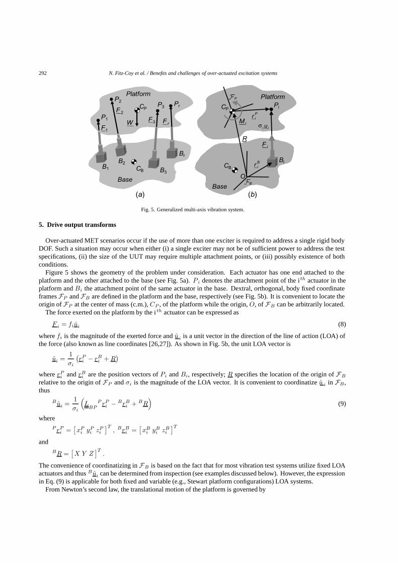
Fig. 5. Generalized multi-axis vibration system.

5. Drive output transforms

Over-actuated MET scenarios occur if the use of more than one exciter is required to address a single rigid bodyDOF. Such a situation may occur when either (i) a single exciter may not be of sufficient power to address the testspecifications, (ii) the size of the UUT may require multiple attachment points, or (iii) possibly existence of bothconditions.

Figure 5 shows the geometry of the problem under consideration. Each actuator has one end attached to theplatform and the other attached to the base (see Fig. 5a). P i denotes the attachment point of the ith actuator in theplatform and Bi the attachment point of the same actuator in the base. Dextral, orthogonal, body fixed coordinateframes FP and FB are defined in the platform and the base, respectively (see Fig. 5b). It is convenient to locate theorigin of FP at the center of mass (c.m.), CP , of the platform while the origin, O, of FB can be arbitrarily located.

The force exerted on the platform by the i th actuator can be expressed as

F i = fiui (8)

where fi is the magnitude of the exerted force and u i is a unit vector in the direction of the line of action (LOA) ofthe force (also known as line coordinates [26,27]). As shown in Fig. 5b, the unit LOA vector is

ui =1σi

(rPi − rBi + R

)where rPi and rBi are the position vectors of Pi and Bi, respectively; R specifies the location of the origin of FB

relative to the origin of FP and σi is the magnitude of the LOA vector. It is convenient to coordinatize u i in FB ,thus

Bui =1σi

(LBP

P rPi − BrBi + BR)

(9)

whereP rPi =

[xPi yPi zPi

]T, BrBi =

[xBi yBi zBi

]Tand

BR =[X Y Z

]T.

The convenience of coordinatizing in FB is based on the fact that for most vibration test systems utilize fixed LOAactuators and thus Bui can be determined from inspection (see examples discussed below). However, the expressionin Eq. (9) is applicable for both fixed and variable (e.g., Stewart platform configurations) LOA systems.

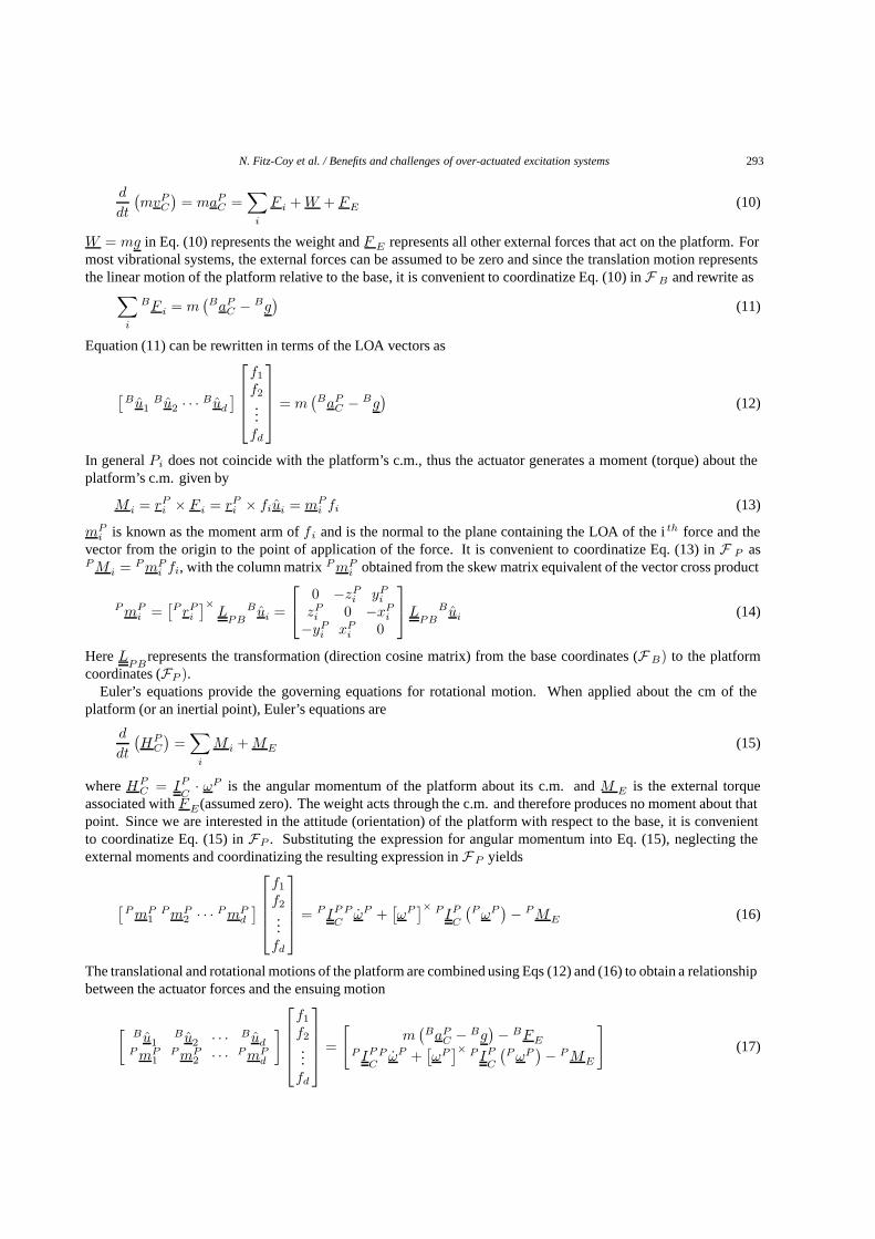
From Newton’s second law, the translational motion of the platform is governed by


d

dt

(mvPC

)= maPC =

∑i

F i + W + FE (10)

W = mg in Eq. (10) represents the weight and F E represents all other external forces that act on the platform. Formost vibrational systems, the external forces can be assumed to be zero and since the translation motion representsthe linear motion of the platform relative to the base, it is convenient to coordinatize Eq. (10) in F B and rewrite as∑

i

BF i = m(BaPC − Bg

)(11)

Equation (11) can be rewritten in terms of the LOA vectors as

[Bu1

Bu2 · · · Bud]f1

f2

...fd

= m

(BaPC − Bg

)(12)

In general Pi does not coincide with the platform’s c.m., thus the actuator generates a moment (torque) about theplatform’s c.m. given by

M i = rPi × F i = rPi × fiui = mPi fi (13)

mPi is known as the moment arm of fi and is the normal to the plane containing the LOA of the i th force and the

vector from the origin to the point of application of the force. It is convenient to coordinatize Eq. (13) in F P asPM i = PmP

i fi, with the column matrix PmPi obtained from the skew matrix equivalent of the vector cross product

PmPi =

[P rPi

]×LPB

Bui =

0 −zPi yPi

zPi 0 −xPi−yPi xPi 0

L

PBBui (14)

Here LPB

represents the transformation (direction cosine matrix) from the base coordinates (F B) to the platformcoordinates (FP ).

Euler’s equations provide the governing equations for rotational motion. When applied about the cm of theplatform (or an inertial point), Euler’s equations are

d

dt

(HP

C

)=

∑i

M i + ME (15)

where HPC = IP

C· ωP is the angular momentum of the platform about its c.m. and M E is the external torque

associated with FE(assumed zero). The weight acts through the c.m. and therefore produces no moment about thatpoint. Since we are interested in the attitude (orientation) of the platform with respect to the base, it is convenientto coordinatize Eq. (15) in FP . Substituting the expression for angular momentum into Eq. (15), neglecting theexternal moments and coordinatizing the resulting expression in FP yields

[PmP

1PmP

2 · · · PmPd

]f1

f2

...fd

= P IP

CP ωP +

[ωP

]× P IPC

(PωP

) − PME (16)

The translational and rotational motions of the platform are combined using Eqs (12) and (16) to obtain a relationshipbetween the actuator forces and the ensuing motion

[Bu1

Bu2 · · · BudPmP

1PmP

2 · · · PmPd

]f1

f2

...fd

=

[m

(BaPC − Bg

) − BFEP IP

CP ωP +

[ωP

]× P IPC

(PωP

) − PME

](17)


Equation (17) is of the form

[P ](6×d)

[F ](d×1)

= [C](6×1)

(18)

where [P ] is a matrix of line coordinates and moment arms which is referred to as the matrix of Plucker coordinates [26,27], [F ] is a matrix of actuator force magnitudes, and [C] is the matrix of the desired motion command (i.e., thegeneralized inertia force).

Equation (18) can be interpreted in the following manner – given the desired motion [C], determine the actuatorforce commands [F ] required to generate that motion. There are two cases of interest, under-actuated (d � m) andover-actuated (d > m) systems where m � 6 in both cases. We examine each case separately.

5.1. Under-actuated system

In Ref. [23] a singular value decomposition (SVD) analysis was used to show that the under-actuated cased < m � 6 actuators have, at most, control authority over d dofs (i.e., d actuators can at best excite d dofs in acontrollable manner). The analysis is repeated here for completeness.

Via the SVD, [P ] can be represented as [P ] = UΣV T , where U and V are respectively, (6 × 6) and (d×d) unitarymatrices. Assuming that [P ] has full column rank (i.e., there are no redundant actuators), then Σ has the form

Σ =[diag (σ1, · · · , σd)

0

]}d

}6−d

Substituting [P ] = UΣV T into Eq. (18) and premultiplying both sides by U T yields[diag (σ1, · · · , σr)

0

]V T [F ] = UT [C] (19)

where one observes that the lower (6 − d) rows of Eq. (19) are zero. This suggests Eq. (19) can be partitioned as[PU

PL

][F ] =

[CU

CR

](20)

where the desired motion is given by [PU ] [F ] = [CU ] and the actuator commands are uniquely determined since[PU ] is full rank. The lower partition, [PL] [F ] = [CR], describes residual motion that may occur; typically thismotion is zero, but if it does occur, it is NOT controllable. Since the actuator commands are linearly independent,the required input transform is the identity matrix.

It should be noted that if [P ] does not have full column rank, then the system is over-actuated (i.e., the inputcommands are not linearly independent) and those cases are discussed below.

5.2. Over-actuated system

For an over-actuated system (d > m), the partitioning of the Plucker matrix as discussed above does not occursince its rank is now based on row rather than columns. For these systems, the drive commands for the d actuatorforce inputs are not linearly independent and are related to a linearly independent set of m drive commands by

[F ](d × 1)

= [P ](d × m)

T [D](m × 1) (21)

Here [D] is the m (� 6) independent drive commands, [F ] is the d > m dependent drive commands, and [P ] T isreferred to in the literature as the “drive output transform” [4]. Substituting into Eq. (18), the independent drivecommand can be determined from the motion command as

[D] =([P ] [P ]T

)−1

[C] (22)

which can then be substituted into Eq. (21) to determine the dependent actuation force levels from


Actuator 2Actuator 1

Pivot

Accelerometer 1

Accelerometer 2

Beam

x

X

Y

Z

y

z

O

1( )l

2( )l

θ1f

2f1r

2r

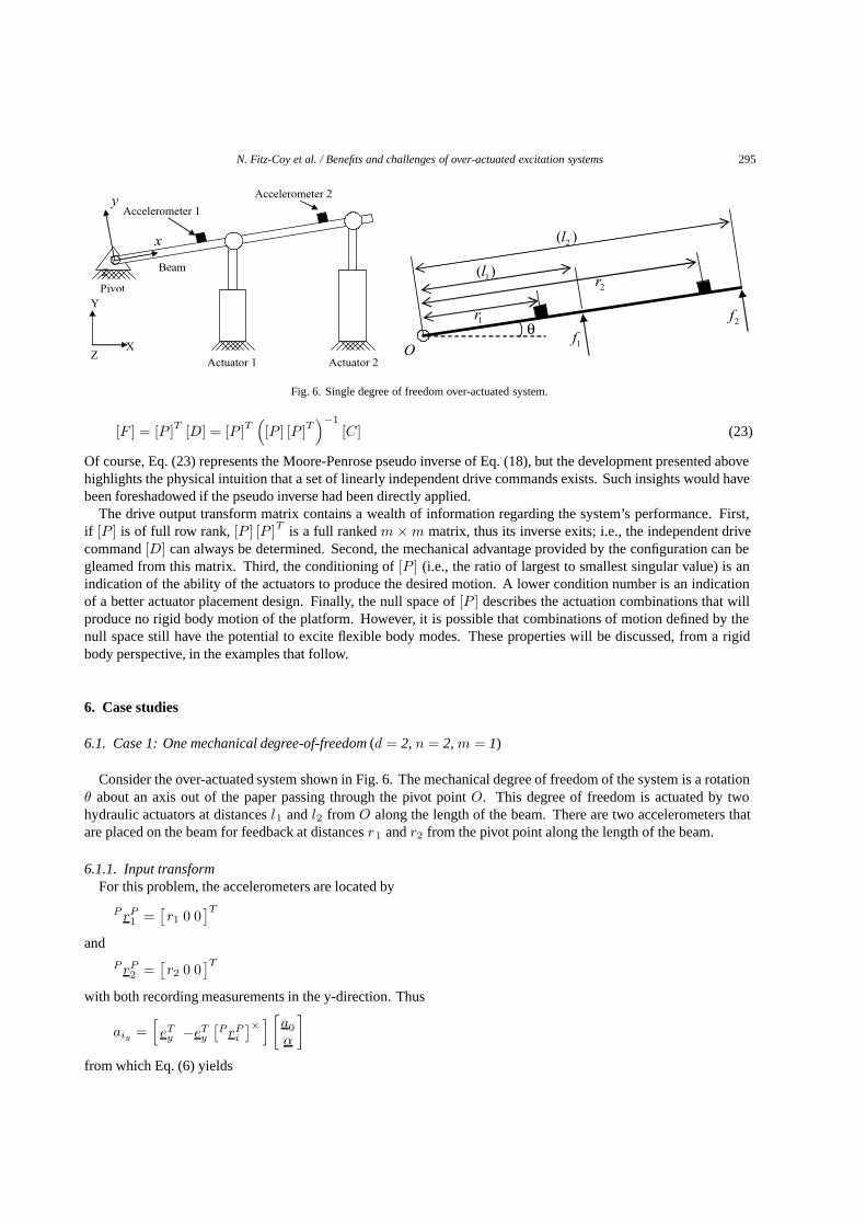
Fig. 6. Single degree of freedom over-actuated system.

[F ] = [P ]T [D] = [P ]T([P ] [P ]T

)−1

[C] (23)

Of course, Eq. (23) represents the Moore-Penrose pseudo inverse of Eq. (18), but the development presented abovehighlights the physical intuition that a set of linearly independent drive commands exists. Such insights would havebeen foreshadowed if the pseudo inverse had been directly applied.

The drive output transform matrix contains a wealth of information regarding the system’s performance. First,if [P ] is of full row rank, [P ] [P ]T is a full ranked m× m matrix, thus its inverse exits; i.e., the independent drivecommand [D] can always be determined. Second, the mechanical advantage provided by the configuration can begleamed from this matrix. Third, the conditioning of [P ] (i.e., the ratio of largest to smallest singular value) is anindication of the ability of the actuators to produce the desired motion. A lower condition number is an indicationof a better actuator placement design. Finally, the null space of [P ] describes the actuation combinations that willproduce no rigid body motion of the platform. However, it is possible that combinations of motion defined by thenull space still have the potential to excite flexible body modes. These properties will be discussed, from a rigidbody perspective, in the examples that follow.

6. Case studies

6.1. Case 1: One mechanical degree-of-freedom (d = 2, n = 2, m = 1)

Consider the over-actuated system shown in Fig. 6. The mechanical degree of freedom of the system is a rotationθ about an axis out of the paper passing through the pivot point O. This degree of freedom is actuated by twohydraulic actuators at distances l1 and l2 from O along the length of the beam. There are two accelerometers thatare placed on the beam for feedback at distances r1 and r2 from the pivot point along the length of the beam.

6.1.1. Input transformFor this problem, the accelerometers are located by

P rP1 =[r1 0 0

]Tand

P rP2 =[r2 0 0

]Twith both recording measurements in the y-direction. Thus

aiy =[eTy −eTy

[P rPi

]× ] [a0

α

]

from which Eq. (6) yields


[a1y

a2y

]=

[0 1 0 0 0 r10 1 0 0 0 r2

] [a0

α

]

By choosing the reference point as the pivot point, then a0 ≡ 0 and thus the first three columns of the coefficient

matrix can be eliminated. Further, since α =[0 0 αz

]T, columns four and five of the coefficient matrix can also be

eliminated which results in[a1y

a2y

]=

[r1r2

]αz

Thus,[I]

=[r1r2

]from which the Input Transform matrix is determined as

[I] =([I]T [I])−1 [I]T =

[r1

r21+r2

2

r2r21+r2

2

]

6.1.2. Drive output transformFor this problem, the relevant geometric properties for the input forces are:

P rP1 =[l1 0 0

]T, P rP2 =

[l2 0 0

]T,Bu=

1

[0 1 0

]T,Bu=

2

[0 1 0

]T.

The moment arm of each actuator about the pivot point (a fixed point) is

PmPi =

[P rPi

]×LPB

Bui =

0 0 0

0 0 −li0 li 0

cos θ sin θ 0− sin θ cos θ 0

0 0 1

0

10

=

0

0li cos θ

0

0li

Since only rotational motion exists, the translational components of Eq. (17) can be neglected to get

[PmP

1PmP

2

] [f1

f2

]=

0 0

0 0l1 l2

[

f1

f2

]= PJP

OP ω +

[Pω

]× PJP

OPω + m

[P rPc

]× P g

where P rPc defines the position of the platform’s c.m. with respect to the pivot point and P g = g[sin θ cos θ 0

]Tis

the gravity vector coordinatized in FP . The third term on the right represents the contribution of the platform’s massto the angular momentum about point ‘O’. In the previous developments this term was zero because the momentswere computed about the c.m thus eliminating its contributions. However, in this example the moments weredetermined about the pivot point (an inertial point), the contribution of the weight to the moment about that pointmust be included. Observe that the first two rows of the Plucker matrix are associated with the x- and y-rotationaldofs and can be ignored since such motions are constrained (as shown by the equation). Thus, [P ] =

[l1 l2

]from

which the drive command is

[D] =([P ] [P ]T

)−1

[C] =([

l1 l2] [

l1l2

])−1 [Jz θ + mglc cos θ

]

=1

l21 + l22[Jzωz + mglc cos θ]

The Drive Output transform [P ]T =[l1l2

]and the actuation level is

[F ] =[f1

f2

]= [P ]T [D] =

1l21 + l22

[l1l2

] [Jz θ + mglc cos θ

](24)

The mechanical advantage of the configuration is l 21 + l22 and is inferred from [P ] [P ]T .


(a) (b)

Fig. 7. Geometry: (a) Actuator and sensor positions [4], (b) Position vectors.

6.2. Case 2: Six mechanical degrees-of-freedom

The example below is from Ref [4]. The geometry for the example is shown in Fig. 7 from which the followingdefinitions were extracted.

P rP1 = P rP8 =[− l l 0

]T, P rP2 = P rP6 =

[l −l 0

]T, P rP3 = P rP5 =

[l l 0

]T, P rP4 = P rP7 =

[−l −l 0]T

Bu1 =[1 0 0

]T,Bu2 =

[−1 0 0]T

,Bu3 =[0 −1 0

]T,Bu4 =

[0 1 0

]TBu5 = Bu6 = Bu7 = Bu8 =

[0 0 1

]TIt should be noted that while this example discusses co-located actuation and measurement points, co-location is nota requirement of the formulation. By this we mean the positions vectors for the accelerometer locations do not haveto be the same as that define the actuator positions. In practice co-located sensors and actuators maybe helpful introuble-shooting but is not required.

6.2.1. Input transformIn this configuration, single axis accelerometers are aligned with the actuators; e.g., at the upper right corner

defined by vector rP1 has accelerometers that record measurements in negative y-direction and the positive z-direction.Using the formulation of Eq. (5) the following component definitions are obtained:

a1x =[eTx −eTx

[P rP1

]× ] [P aPoPαP

]=

[1 0 0 0 0 −1

] [P aPoPαP

]

a2x =[−eTx eTx

[P rP2

]× ] [P aPoPαP

]=

[ −1 0 0 0 0 −1] [

PaPoPαP

]

a3y =[−eTy eTy

[P rP3

]× ] [P aPoPαP

]=

[0 −1 0 0 0 −1

] [PaPoPαP

]

a4y =[eT2 −eT2

[P rP4

]× ] [P aPoPαP

]=

[0 1 0 0 0 −1

] [P aPoPαP

]

a5z =[eT3 −eT3

[P rP5

]× ] [PaPoPαP

]=

[0 0 1 1 −1 0

] [PaPoPαP

]

a6z =[eT3 −eT3

[P rP6

]× ] [PaPoPαP

]=

[0 0 1 −1 −1 0

] [PaPoPαP

]


a7z =[eT3 −eT3

[P rP7

]× ] [PaPoPαP

]=

[0 0 1 −1 1 0

] [PaPoPαP

]

a8z =[eT3 −eT3

[P rP8

]× ] [PaPoPαP

]=

[0 0 1 1 1 0

] [PaPoPαP

]

Combining these components as shown in Eq. (6) gives an[I]

which yields the input transform upon inversion

[I] =

0.5 −0.5 0 0 0 0 0 00 0 −0.5 0.5 0 0 0 00 0 0 0 0.25 0.25 0.25 0.250 0 0 0 0.25/l −0.25/l −0.25/l 0.25/l0 0 0 0 −0.25/l −0.25/l 0.25/l 0.25/l

−0.25/l −0.25/l −0.25/l −0.25/l 0 0 0 0

where the first three rows are associated with the x-, y-, and z-translational accelerations, and the last three rows areassociated with the x-, y-, and z-angular accelerations.

6.2.2. Drive output transform

The corresponding input is [F ] =[f1 f2 f3 f4 f5 f6 f7 f8

]Twhere f1 and f2 are in the x-direction forces at

diagonally opposing corners, f3 and f4 are the y-direction forces applied at the corners of the other diagonal, andf5 − f8 are vertical (z-direction) forces. Assuming small angular displacements of the platform, Eq. (14) can beused to obtain

PmP1 =

[lθ lθ −l (1 − ψ)

]T, PmP

2 =[lθ lθ −l (1 − ψ)

]T, PmP

3 =[lϕ lϕ−l (1 − ψ)

]T,

PmP4 =

[lϕ lϕ −l (1 − ψ)

]T, PmP

5 =[l −l l (θ + ϕ)

]T, PmP

6 =[−l −l −l (θ − ϕ)

]T,

PmP7 =

[−l l −l (θ + ϕ)]T

, PmP8 =

[l l l (θ − ϕ)

]TThus, the matrix of Plucker coordinates is

[P ] =

1 −1 0 0 0 0 0 00 0 −1 1 0 0 0 00 0 0 0 1 1 1 1lθ lθ lϕ lϕ l −l −l llθ lθ −lϕ −lϕ −l −l l l

−l(1 − ψ) −l(1 − ψ) −l(1 − ψ) −l(1 − ψ) l(θ + ϕ) −l(θ − ϕ) −l(θ + ϕ) l(θ − ϕ)

The results of Ref [4] assumes the angular displacements are zero, so to be consistent we apply the same conditionsto reduce the matrix of Plucker coordinates to

[P ] =

1 −1 0 0 0 0 0 00 0 −1 1 0 0 0 00 0 0 0 1 1 1 10 0 0 0 l −l −l l0 0 0 0 −l −l l l−l −l −l −l 0 0 0 0

from which the Drive Output transform is determined as

[P ]T =

1 0 0 0 0 −l−1 0 0 0 0 −l0 −1 0 0 0 −l0 1 0 0 0 −l0 0 1 l −l 00 0 1 −l −l 00 0 1 −l l 00 0 1 l l 0


For the drive output transform shown above, the first three columns are associated, respectively, with the x-, y-, andz-translational dofs and the last three columns are associated with the x-, y-, and z-rotational dofs of the platform.With considerations for the appropriate physical degrees of freedom, the drive output transform shown in Eq. (3) ofRef. [4] is identical to that shown above.

The mechanical advantage provided by the configuration is obtained from an evaluation of [P ] [P ] T . For thisexample, we have

[P ] [P ]T = diag[

2 2 4 4l2 4l2 4l2]

which indicates that there is a mechanical advantage of 2 for the x- and y-translational dofs and an advantage of4 for the z-translation and all three rotational dofs. Of course this result could have been discerned from carefulexamination of the actuator configuration.

For this example, the null space of [P ] contains the following two vectors:

[F ]null1 =[

0 0 0 0 0.5 −0.5 0.5 −0.5]T [F ]null2 =

[0.5 0.5 −0.5 −0.5 0 0 0 0

]TIn terms of rigid body motion, the scenario defined by the first null vector results in the four base actuators producingzero vertical force, pitch, and roll moments. Similarly, that of the second null vector involves the planar actuatorsproducing no net horizontal forces and no yaw moment. Again, it is important to recognize that null space excitationhas the potential to excite flexible body DOFs. Specific to this example, [F ]null1 corresponds to vertical actuatorsthat are 180 degrees out of phase with respect to each other which may result in torsional deformation of the platformand [F ]null2 corresponds to out of phase horizontal exciters which may result in shear deformation of the table, asdiscussed in [4].

6.3. Case 3: One mechanical degree-of-freedom with phase difference

The purpose of this example is to highlight the effects of actuator phase difference on the performance of thesystem. This is demonstrated by considering sinusoidal inputs f1 and f2 which cause displacements y1 and y2 at theactuator attachment points of example Case 1. To further highlight these effects, we consider two different actuationsystems: (i) electrodynamic actuation and (ii) hydraulic actuation (Fig. 6).

In the case of ideal actuators that can be phase matched, it is possible that the forces are in phase and follow therelationship as given by Eqs (24), (25) provide the actuation conditions for rigid body motion (neglecting inertiaeffects).

f1 = F1 sin(ωf t)

f2 = F2 sin(ωf t)

y1 = Y1 sin(ωt)

y2 = Y2 sin(ωt)(25)

where ωf is the frequency of actuation, Y1 and Y2 are the peak displacements consistent with the motion. However,for realizable systems, it is difficult to phase match the actuators and thus the imparted forces will have some phase,differences and produce displacements which may not be consistent with rigid body motion. The motion of theattachment points become functions of generalized displacement functions q 1 and q2 given by

f1 = F1 sin(ωf t)f2 = F2 sin(ωf t + ϕ)

y1 = q1(ωf , ϕ, E, I, F1, F2)y2 = q2(ωf , ϕ, E, I, F1, F2)

(26)

where ϕ represents the actuation phase difference, E and I are the beam’s Young’s modulus and its second momentof the cross-sectional area.

This difference in displacement will cause structural deformations in the beam leading to high actuator forces andexcitation of some modes of the beam.

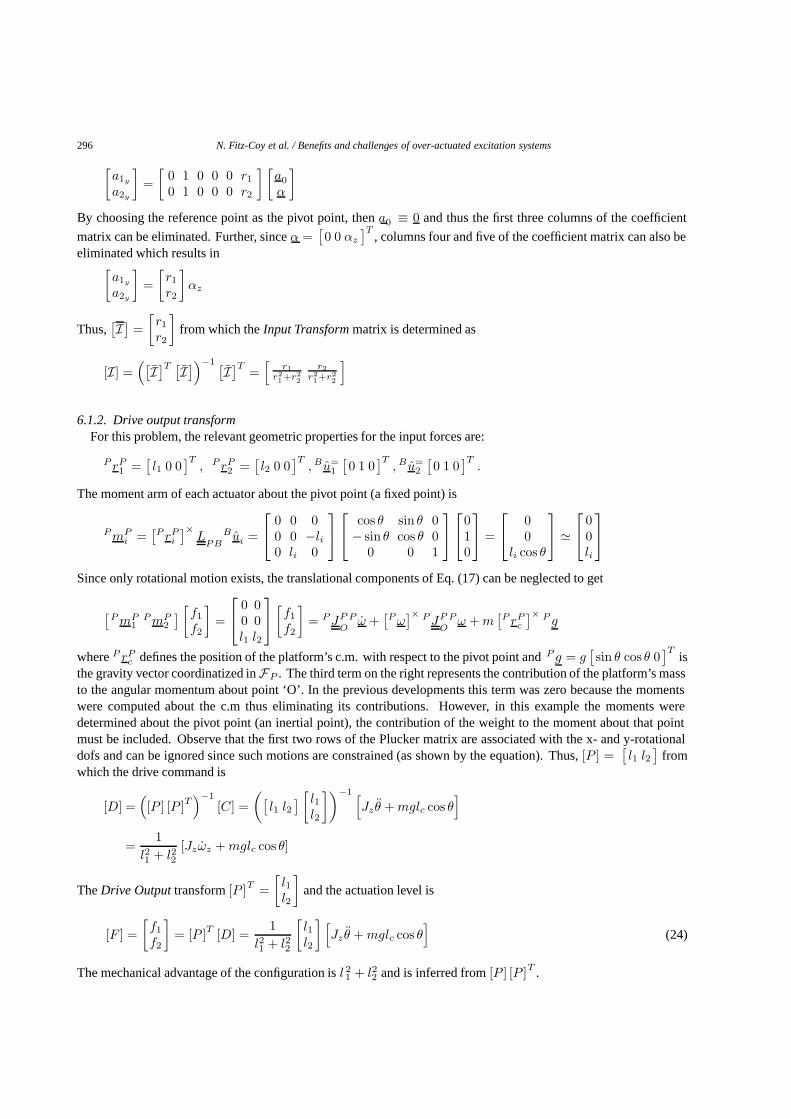
Figure 8 in considers two cases of actuation of a beam – one by an electrodynamic actuator and the other by ahydraulic shaker.

In the common case let the forces by actuators 1 and 2 at distances l 1 and l2 cause displacements y1 and y2 atthe attachment points. If y1 = (l1/l2) y2, which is the condition for rigid body motion then the beam has to flex tocomply with the displacements. For the electrodynamic actuator case, the magnet field/armature acts as a compliant


(A) (B)

Actuator 1 Actuator 2

1Ey s

2Ey s−∆

+∆

Fig. 8. Comparison between (a) Electrodynamic and (b) Hydraulic actuators.

spring that would compensate for the displacement difference and does not let the beam to deform. Due to thecompliance of the spring, y1 will now be equal to y1 = (yE1 + ∆s) = (l1/l2) (yE2 − ∆s). The additional force onthe beam would be only k (∆s) where k is the stiffness of the beam.

For the case of the hydraulic oil column is stiff and not compliant enough to avoid considerable beam deformations.This causes the beam to deflect by the difference in displacements between the rigid body motion to the actualdisplacement. The additional force now is considerable as the bending stiffness of the beam is high. This additionalforce on the actuator may also damage the valves in the hydraulic circuit.

A test case with the following specifications of the beam was simulated in ADAMS software [28].Beam length: 1mBeam cross-section: 0.05 m × 0.05 mBeam material: steelDensity of the beam: 7800 Kg/m3

Young modulus: 210 GpaPosition of the actuators: l1 = 0.4m and l2 = 0.8mIn the first case the actuator was modeled with a spring in series to simulate the electrodynamic actuator. The

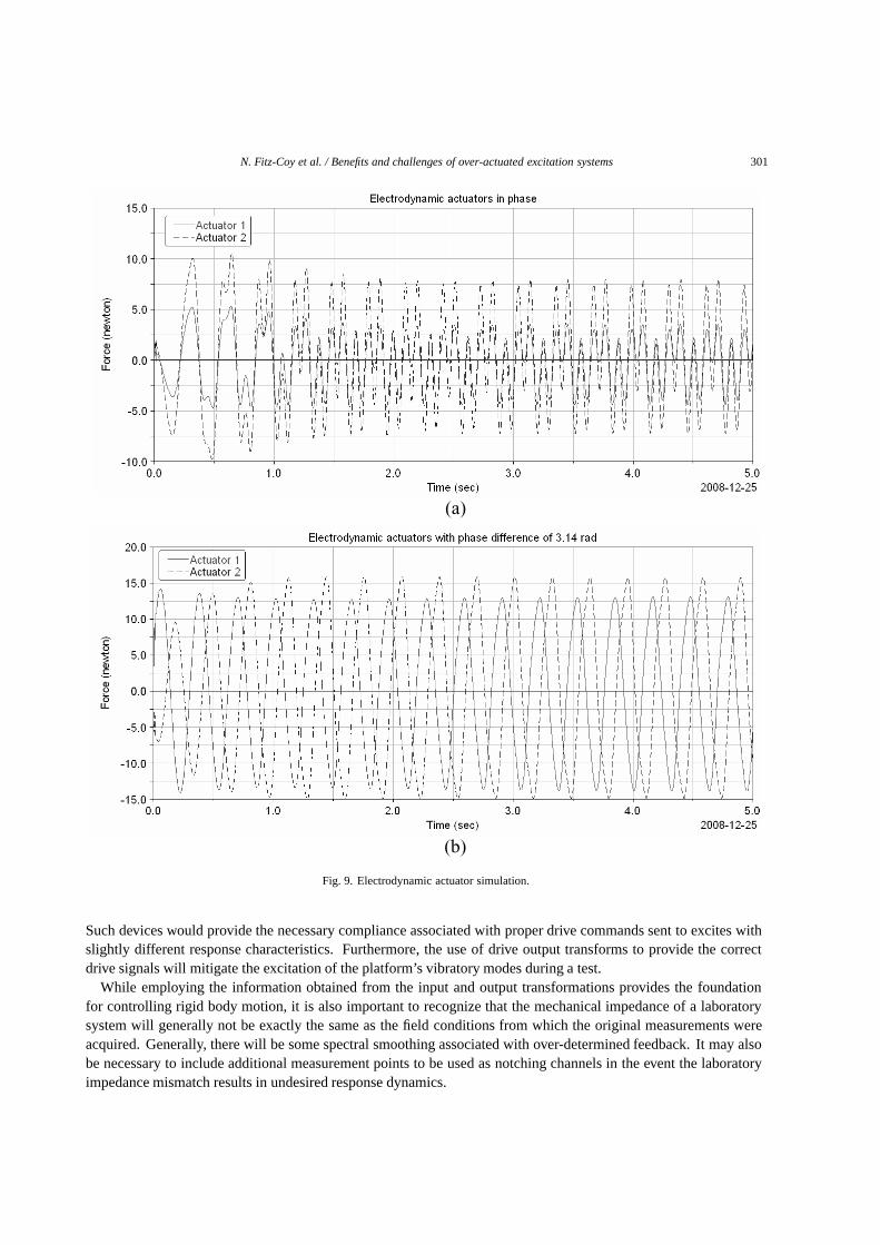
stiffness of the spring used was 10N/mm with a damping ratio of 0.1. Figure 9 shows the plot of the forces at theelectrodynamic actuator joints when the actuators are (a) in phase and (b) out of phase by π radians.

The simulation was repeated with the springs replaced by a rigid member to represent the hydraulic actuator.Figure 10 shows the plot of the forces at the hydraulic actuator joints when the actuators are (a) in phase and (b) outof phase by π radians.

It is evident from the above plots that there is an enormous increase in the forces at the actuator joints due tothe flexure of the beam in case of a hydraulic actuator. This problem does not occur in case of an electrodynamicactuator due to the compliance by the actuator springs.

7. Discussions and conclusions

In this paper we have motivated the need for over-actuated vibration control systems and discussed the challengesthat are present in multi-axis vibration systems. The relationships between the desired vibrational motion and theactuation required to generate that motion is developed from a mechanics perspective and used to highlight thechallenges that exist for these systems. Based on these relationships, we have shown that a drive output transformis not required for under-actuated systems but is essential for over-actuated. Due to the use of electro-dynamicactuators, the need for drive output transforms in over-actuated systems were not as critical since the actuator itselfprovide the compliance required if the drives were not synchronized. However, as the use of hydraulic actuatorsbecome more prevalent in these over-actuated systems, it will be imperative that such transforms be integrated intothe development of the control systems since these actuators will not provide the necessary compliance. Actuatordevelopers are currently investigating passive methods for providing some compliance (e.g., TEAM’s delta-P valve),however, such devices will not in principle provide the necessary compliance required for over-actuated systems.


(a)

(b)

Fig. 9. Electrodynamic actuator simulation.

Such devices would provide the necessary compliance associated with proper drive commands sent to excites withslightly different response characteristics. Furthermore, the use of drive output transforms to provide the correctdrive signals will mitigate the excitation of the platform’s vibratory modes during a test.

While employing the information obtained from the input and output transformations provides the foundationfor controlling rigid body motion, it is also important to recognize that the mechanical impedance of a laboratorysystem will generally not be exactly the same as the field conditions from which the original measurements wereacquired. Generally, there will be some spectral smoothing associated with over-determined feedback. It may alsobe necessary to include additional measurement points to be used as notching channels in the event the laboratoryimpedance mismatch results in undesired response dynamics.


(a)

(b)

Fig. 10. Hydraulic actuator simulation.

References

[1] K.A. Edge, The Control of Fluid Power Systems – Responding to the Challenges, Proc. Institution of Mechanical. Engineers, Part I: J.Systems and Control Engineering, 1996, 211, 91–110.

[2] M. Tochizawa and K.A. Edge, A Comparison of Some Control Strategies for a Hydraulic Manipulator, Proc. Of the American ControlsConference, San Diego, California June 1999, pp. 744–748.

[3] T. Davis, Multiple-Input, Multiple-Output (MIMO) Control Systems – A New Era in Shaker Control, Sound and Vibration (Jan. 2006).[4] M. Underwood and T. Keller, Applying Coordinate Transformations to Multi-DOF Shaker Control, Sound and Vibration (Jan. 2006),

22–27.[5] F. De Coninck, W. Desmet and P. Sas, Increasing the Accuracy of MDOF Road Reproduction Experiments: Calibration, Tuning and a

Modified TWR Approach, Proc. of the International Conference on Noise and Vibration Engineering, Sept. 2004, pp. 709–722.


[6] J. Zhao, C. French, C. Shield and T. Posbergh, Considerations for the development of real-time dynamic testing using servo-hydraulicactuation, Earthquake Engineering Structural Dynamics 32 (2003), 1773–1794.

[7] J. Zhao, C. Shield, C. French and T. Posbergh, Effect of Servo Valve/Actuator Dynamics on Displacement Controlled Testing, Presented atthe 13th World Conference on Earthquake Engineering, Vancouver, B.C., Canada, August 1–6, 2004, Paper No. 267.

[8] H. Hahn and K.-D. Leimbach, Nonlinear Control and Sensitivity Analysis of A Spatial Multi-Axis Servo-Hydraulic Test Facility, Proc. Ofthe 32nd Conference on Decision and Control, San Antonio TX, Dec. 1993, 116–1123.

[9] Y. Uchiyama, M. Mukai and M. Fujita, Robust Control of Multi-Axis Shaking System Using µ-Synthesis, Proc. of the 16th IFAC WorldCongress on Automatic Control, Prague, Czech, July 2005.

[10] J.N. Fletcher, H. Vold and M.D. Hansen, Enhanced Multiaxis Vibration Control Using a Robust Generalized Inverse System Matrix, J ofthe IES 38(2) (March-April 1995), 36–42.

[11] M. Chen and D.R. Wilson, The New Triaxial Shock and Vibration Test System at Hill Air Force Base, J of the IEST 41(2) (March-April1998), 27–32.

[12] N. Uchiyama, S. Takagi, S. Sano and K. Yamazaki, Robust Contouring Control for Multi-Axis Feed Drive Systems, 2006, pp. 840–845.[13] A. Steinwolf and W.H. Connon III, Limitations of the Fourier Transform for Describing Test Course Profiles, Sound and Vibration, Feb.

2005 (Instrumentation Reference Issue), pp. 12–17.[14] A.R. Plummer, Control techniques for structural testing: a review, Proc. of the Institute of Mechanical Engineering Part I Journal of

Systems & Control Engineering 221(2) (2007), 139–169.[15] A.O. Gizatullin and K.A. Edge, Adaptive control for a multi-axis hydraulic test rig, Proc. of the Institute of Mechanical Engineering Part

I Journal of Systems & Control Engineering 221(2) (2007), 183–198.[16] Y. Tagawa and K. Kajiwara, Controller development for the E-Defense shaking table, Proc. of the Institute of Mechanical Engineering

Part I Journal of Systems & Control Engineering 221(2) (2007), 171–181.[17] A.R. Plummer, Modal control for a class of multi-axis vibration table, Proc. Of the UKACC Control 2004 Mini Symposia, Bath, UK, Sept.

2004. pp. 111–115.[18] D.O. Smallwood, Multiple Shaker Random Vibration Control – An Update, Proc. of the IEST, 1999.[19] J.J. Dougherty and H. El-Sherief, Modeling and identification of a triaxial shaker control system, Proceedings of the 4th IEEE Conference

on Control Applications, Sept. 1995, pp. 884–889.[20] B. Peters and J. Debille, MIMO Random Vibration Control Algorithms and Simulations, 72nd Shock and Vibration Symposium.[21] M. Underwood and T. Keller, Recent System Developments for Multi-Actuator Vibration Control, Sound & Vibration, Oct. 2001.[22] Team Corporation, Technical Note on Sizing a Hydraulic Shaker, 1990.[23] N. Fitz-Coy and D. McDaniel, An Analysis of Multi-Axis Vibration Simulators, Presented at the 64th Shock & Vibration Symposium, Ft.

Walton Beach, Nov. 1993.[24] Hale and N. Fitz-Coy, On the Use of Linear Accelerometers in Six-DOF Laboratory Motion Replication: A Unified Time-Domain Analysis,

presented at the 76th Shock & Vibration Symposium, Destin FL, 2005.[25] P. Hughes, Spacecraft Attitude Dynamics, John Wiley, and Sons, 1986, pp. 27–29.[26] E.F. Fitcher, A Stewart Platform-Based Manipulator: General Theory and Practical Considerations, The International Journal of Robotics

Research 5(2) (1986), 157–182.[27] K.H. Hunt, Kinematic Geometry of Mechanisms, Oxford University Press, Oxford, 1978.[28] http://www.mscsoftware.com/assets/Adams DS.pdf.

International Journal of

AerospaceEngineeringHindawi Publishing Corporationhttp://www.hindawi.com Volume 2010

RoboticsJournal of

Hindawi Publishing Corporationhttp://www.hindawi.com Volume 2014


Active and Passive Electronic Components

Control Scienceand Engineering

Journal of



RotatingMachinery


Hindawi Publishing Corporation http://www.hindawi.com

Journal ofEngineeringVolume 2014

Submit your manuscripts athttp://www.hindawi.com

VLSI Design



Shock and Vibration


Civil EngineeringAdvances in

Acoustics and VibrationAdvances in



Electrical and Computer Engineering

Journal of

Advances inOptoElectronics

Hindawi Publishing Corporation http://www.hindawi.com

Volume 2014

The Scientific World JournalHindawi Publishing Corporation http://www.hindawi.com Volume 2014

SensorsJournal of


Modelling & Simulation in EngineeringHindawi Publishing Corporation http://www.hindawi.com Volume 2014


Chemical EngineeringInternational Journal of Antennas and

Propagation




Navigation and Observation



DistributedSensor Networks


Documents

Beneﬁts and challenges of over-actuated excitation systems